Download - IandF CT3 201509 ExaminersReport

7/24/2019 IandF CT3 201509 ExaminersReport

http://slidepdf.com/reader/full/iandf-ct3-201509-examinersreport 1/12

INSTITUTE AND FACULTY OF ACTUARIES

EXAMINERS’ REPORT

September 2015

Subject CT3 – Probability and

Mathematical StatisticsCore Technical

Introduction

The Examiners’ Report is written by the Principal Examiner with the aim of helping candidates, both

those who are sitting the examination for the first time and using past papers as a revision aid and

also those who have previously failed the subject.

The Examiners are charged by Council with examining the published syllabus. The Examiners have

access to the Core Reading, which is designed to interpret the syllabus, and will generally base

questions around it but are not required to examine the content of Core Reading specifically or

exclusively.

For numerical questions the Examiners’ preferred approach to the solution is reproduced in this

report; other valid approaches are given appropriate credit. For essay-style questions, particularly the

open-ended questions in the later subjects, the report may contain more points than the Examiners

will expect from a solution that scores full marks.

The report is written based on the legislative and regulatory context pertaining to the date that theexamination was set. Candidates should take into account the possibility that circumstances may

have changed if using these reports for revision.

F Layton

Chairman of the Board of Examiners

December 2015

Institute and Faculty of Actuaries



Subject CT3 (Probability and Mathematical Statistics Core Technical) – September 2015 – Examiners’ Report

A. General comments on the aims of this subject and how it is marked

1. The aim of the Probability and Mathematical Statistics subject is to provide a grounding in

the aspects of statistics and in particular statistical modelling that are of relevance to

actuarial work.

2. Some of the questions in this paper admit alternative solutions from these presented in

this report, or different ways in which the provided answer can be determined. All

mathematically correct and valid alternative solutions or answers received credit as

appropriate.

3. Rounding errors were not penalised, unless excessive rounding led to significantly

different answers.

4. In cases where the same error was carried forward to later parts of the answer,

candidates were only penalised once.

5. In questions where comments were required, reasonable comments that were different

from those provided in the solutions also received full credit where appropriate.

B. General comments on student performance in this diet of theexamination

1. The performance was generally good, with most questions being well answered.

2. The pass rate was in line with previous sessions and there were a number of excellent

scripts achieving very high scores.

3. In general, questions that required moderate mathematical calculus skills

(e.g. differentiation) were poorly answered.

4. In some parts candidates failed to distinguish between the need for different types of test

(e.g. normal z-test, as opposed to a t-test).

C. Comparative pass rates for the past 3 years for this diet of examination

Year %

September 2015 68

April 2015 66

September 2014 57

April 2014 60

September 2013 64

April 2013 59




Reasons for any signi ficant change in pass rates in current diet to those in the

past:

The pass rate for this examination diet is slightly higher than the April 2015 rate, but not

materially different. Variation in the pass rate between sessions is expected as differentcohorts of students sit the examination – however the increasing rates in recent diets reflect

stronger performance from the candidates.

Solutions

Q1 (i) New sum is (11860 – 770 – 510 + 1000 + 280) = 11860

New sum of squares: (8438200 – 7702 – 5102 + 10002 + 2802) = 8663600

Therefore:

New sample mean = 11860/20 = 593

New standard deviation (sd) = {(8663600 – 118602/20)/19}0.5 = 292.95

(ii) Since the sum of the two new claims is the same as those replaced, the mean is

the same.

However the sd has increased as the two new claims are further away from the

mean as compared to the two claims in the first sample.

Part (i) was generally well answered. In part (ii) the explanation about the sd

was not always convincing.

Q2 (i) We have mean = 1.6/0.2 = 8 and sd = (1.6/0.22)0.5 = 6.325

For the mode we need to maximise the probability density function (pdf):

1

log log log 1 log

y

f y y e

f y y y

and

1 1

log 0d

f y ydy y

.




2

2 2

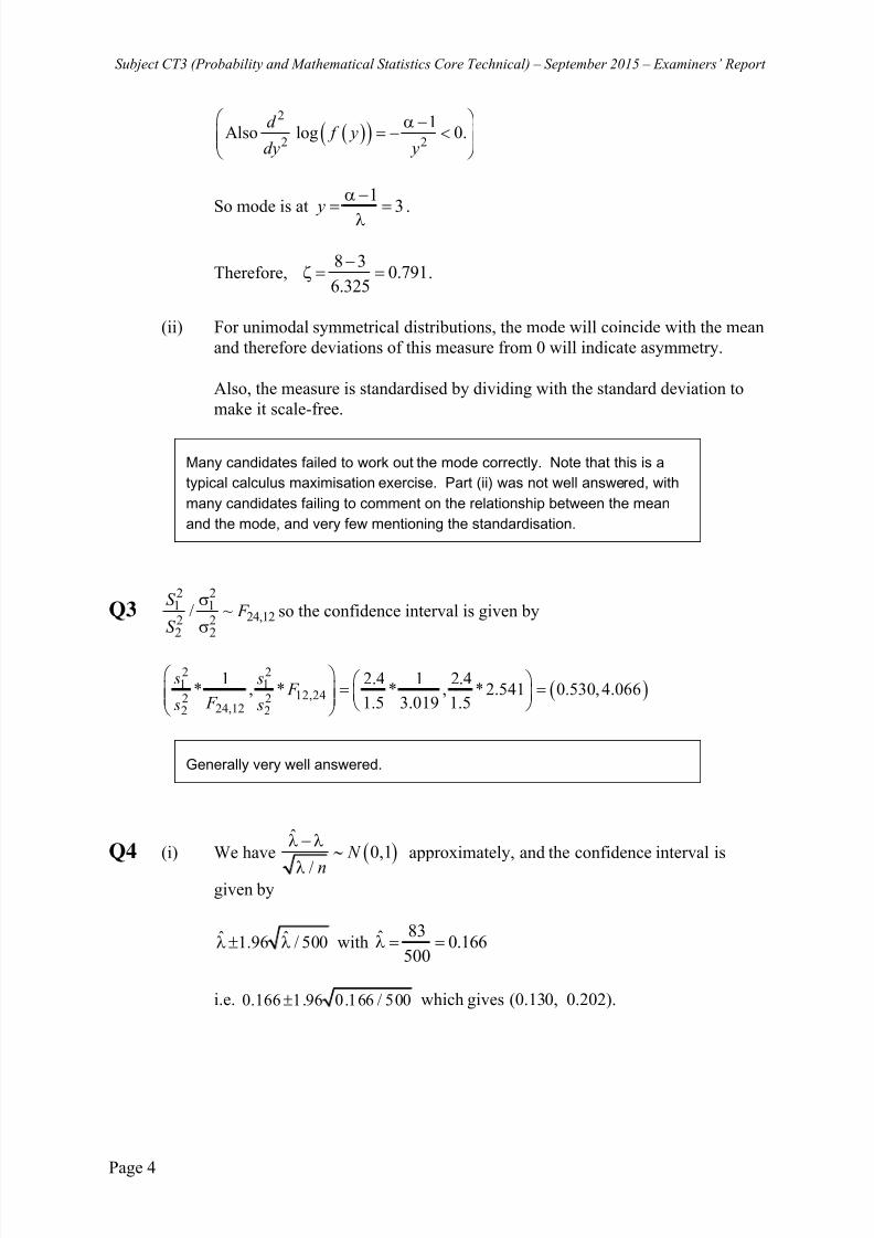
1Also log 0.

d f y

dy y

So mode is at1

3 y

.

Therefore,8 3

0.7916.325

.

(ii) For unimodal symmetrical distributions, the mode will coincide with the mean

and therefore deviations of this measure from 0 will indicate asymmetry.

Also, the measure is standardised by dividing with the standard deviation to

make it scale-free.

Many candidates failed to work out the mode correctly. Note that this is a

typical calculus maximisation exercise. Part (ii) was not well answered, with

many candidates failing to comment on the relationship between the mean

and the mode, and very few mentioning the standardisation.

Q32 21 1

24,122 22 2

/ ~S

F S

so the confidence interval is given by

2 21 1

12,242 224,122 2

1 2.4 1 2.4* , * * , *2.541 0.530, 4.066

1.5 3.019 1.5

s s F

F s s

Generally very well answered.

Q4 (i) We have ˆ

0,1 N

n

approximately, and the confidence interval is

given by

1.96 5 0ˆ ˆ / 0 with83

0.166500

i.e. 0.166 1.96 0.166 / 500 which gives (0.130, 0.202).




(ii) The sample size is large here, so normal approximation is valid.

[Equivalently n λ is large.]

Generally well answered. Some candidates failed to properly justify the use

of the normal approximation.

Q5 (i)2606.96

0.14703265116701 61.44

r

(ii)2

25 2 0.147 230.71

1 0.02161

r t

r

t has t -distribution with 23 d.f. The 95% quantile is 1.714.

Since this is a two-sided test and 0.71 is within the interval [–1.714, 1.714] the

null hypothesis cannot be rejected at 10% level of significance.

(Note that other significance level may also be used.)

[Alternatively, Fisher’s transformation gives z = 0.695, and conclusion is the

same as above.]

Well answered. Note that the test in part (ii) is two-sided.

Q6 2 2 249 7 6 9 8,134 RSS

26 22 2725

3Y

2 2 250 26 25 22 25 27 25 700 BSS

2,147

700 1472 6.3252 8134

147

B

R

SS

F SS

This is clearly a rather large value since the 1% point from a 2,120 F distribution is

4.787, so the null hypothesis is rejected. We conclude that alcohol consumption is

different in different areas.




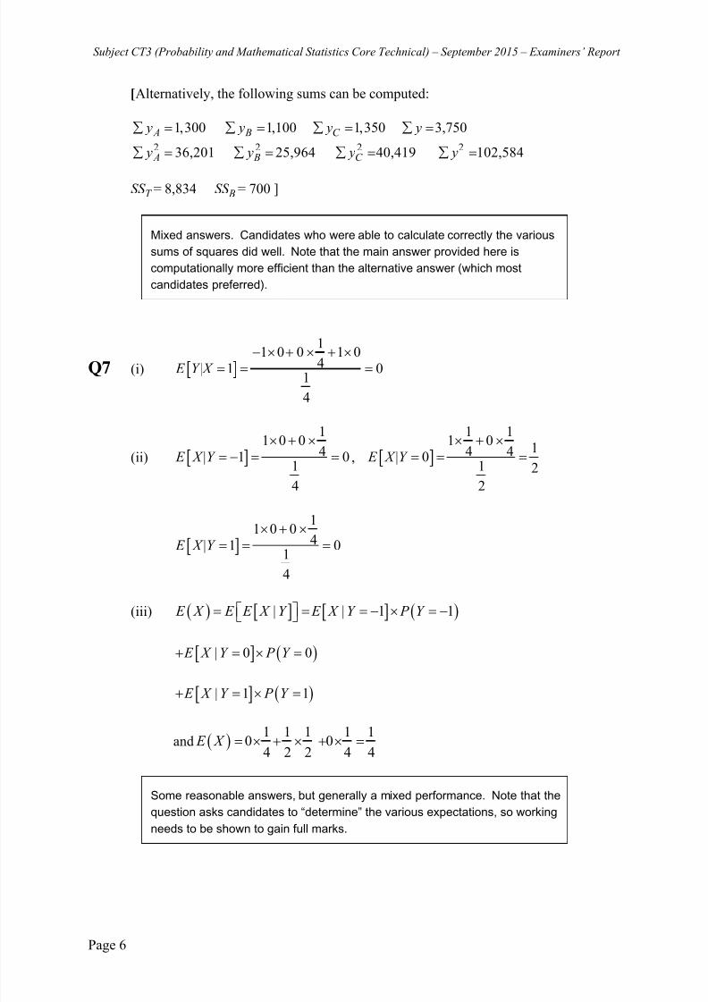
[Alternatively, the following sums can be computed:

1,300 1,100 1,350 3,750 A B C y y y y

2 2 2 236,201 25,964 40,419 102,584 A B C y y y y

SS T = 8,834 SS B = 700 ]

Mixed answers. Candidates who were able to calculate correctly the various

sums of squares did well. Note that the main answer provided here is

computationally more efficient than the alternative answer (which most

candidates preferred).

Q7 (i)

11 0 0 1 0

4| 1 01

4

E Y X

(ii)

11 0 0

4| 1 01

4

E X Y

,

1 11 0

14 4| 01 2

2

E X Y

11 0 04| 1 0

1

4

E X Y

(iii) | | 1 1 E X E E X Y E X Y P Y

| 0 0 E X Y P Y

| 1 1 E X Y P Y

and 1 1 1 1 1

0 04 2 2 4 4

E X

Some reasonable answers, but generally a mixed performance. Note that the

question asks candidates to “determine” the various expectations, so working

needs to be shown to gain full marks.




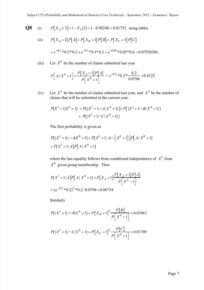
Q8 (i) 2 1 1 1 0.98248 0.01752 A A P X F using tables

(ii) 1 1 1 A B C P X P A P X P B P X P C

0.2 0.1 0.05*0.2*0.2 *0.1*0.2 *0.05*0.6 0.07938286e e e .

(iii) Let 0 X be the number of claims submitted last year

0

0

1| 1

1

A P X P A P A X

P X

=0.2 0.2

*0.2* 0.41250.0794

e

(iv) Let 0 X be the number of claims submitted last year, and 1 X be the number of

claims that will be submitted in the current year.

1 0[ 1 | 1] P X X 1 0 1 0[{ 1 | 1} { 1 | 1}] P X A X P X B X

1 0 [{ 1 | 1}] P X C X

The first probability is given as

1 0 1 0 0[{ 1} | 1] [ 1| 1 | 1] P X A X P X A X P A X

1 0[ 1| | 1] P X A P A X

where the last equality follows from conditional independence of 1 X from0 X given group membership. Then

1 0

0

1[ 1| | 1] 1

1

A A

P X P A P X A P A X P X

P X

0.2 2 ( *0.2) *0.2 / 0.0794 0.06754e

Similarly

21 0

0[{ 1} | 1] 1 0.02062

1 B

P B P X B X P X

P X

21 0

0[{ 1} | 1] 1 0.01709

1C

P C P X C X P X

P X




Thus:

1 0[ 1 | 1] 0.06754 0.02062 0.01709 0.10521 P X X

Part (i) Well answered, although some candidates over-complicated theanswer.

Part (ii) Generally well answered.

Part (iii) Reasonably well answered.

Part (iv) This was not well answered. It is a more challenging question, with

other parts leading up to this. Many candidates did not attempt it.

Q9 (i) (a) Let denote the standard deviation of an estimate. Then we want

0.975 0.975 0.95 P Z X Z

So for the interval width for one observation to be equal to 10 we need:

0.975 0.975 0.9752 2*1.96 10 Z Z Z

52.551

1.96

(b) Let n denote number of satellite passes. Then the estimated survey

height is Normally distributed with variance 2 / .n As before we want

21.96

2 1 3.92 100nn

(ii) Let 1 X and 2 X denote the survey estimates for the two peaks.

Then under 0 H : heights are the same,

2 21 2 ~ 0, 2 / 20 0, /10 D X X N N

P -value is given as:

1.6 or 1.6 2 1.6 2(1 1.6 / / 10 P D D P D P Z

2 1 1.983 2 1 0.976 0.048 P Z




Therefore reject 0 H at the 5% significance level

[Alternatively, the value of the statistic z = 1.983 can be compared with the

normal quantile 1.96.]

(iii) t -test – we assume equal variance as the same system is being used.

2 2 2119*2.5 19*2.6 6.505

20 20 2 P s

test statistic =1.6 1.6

1.9842 1

2.5520 10

P s

test statistic 20 20 2 38~ t t . Quantile is 2.024 at 2.5%.

So do not reject 0 H : no difference in means at 5% significance level.

(iv) Both systems gave the same estimate of difference and almost the same

standard deviation, with the second being lower. However the tests gave

different results.

We did not reject that there was no difference for the test in part (iii) as there

was greater uncertainty since we did not know the standard deviation

beforehand.

Part (i) was generally well answered. As the result is given in the question,

candidates needed to clearly show how to obtain it.

The performance in parts (ii) and (iii) was mixed. Many candidates failed to

demonstrate understanding of which statistic must be used in each of the two

tests, which was one of the main points of the question.

Q10 (i) We have

1

! !

ii i X n X n

i ii i

e e L

X X

and

log log log !i i

i i

l L n X X

and 0 / 0 /ˆi i

i i

d l n X X n X d




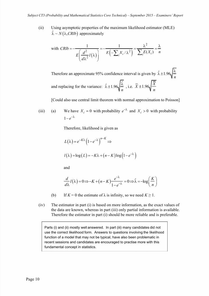
(ii) Using asymptotic properties of the maximum likelihood estimator (MLE)

~ ,ˆ N CRlb approximately

with

2

2 2

2

1 1

( )/ ii ii

CRlb

n E X d E X E l d

Therefore an approximate 95% confidence interval is given by 1.96ˆn

and replacing for the variance: 1.96ˆ

ˆn

, i.e. 1.96

X X

n

[Could also use central limit theorem with normal approximation to Poisson]

(iii) (a) We have 0i X with probability e and 0i X with probability

1 e

Therefore, likelihood is given as

1n K

K L e e

log log 1l L K n K e

and

0 0 loˆ g1

d e K l K n K

d ne

(b) If K = 0 the estimate of λ is infinity, so we need K ≥ 1.

(iv) The estimator in part (i) is based on more information, as the exact values of

the data are known, whereas in part (iii) only partial information is available.

Therefore the estimator in part (i) should be more reliable and is preferable.

Parts (i) and (ii) mostly well answered. In part (iii) many candidates did not

use the correct likelihood form. Answers to questions involving the likelihood

function of a model that may not be typical, have also been problematic in

recent sessions and candidates are encouraged to practise more with this

fundamental concept in statistics.




Q11 (i) Test statistic:2new

24,602old

~S

F S

2 22 2

new

1 1 800 25*4

25 16.6724 25 24i iS x x

22old

2, 200 300 / 61

60S

= 12.08

The 95% quantile of F 24,60 is 1.7 and observed value is

16.67 1.38 1.712.08

F

Therefore, there is no evidence (at 5% level) to suggest that the variance for

new buildings is larger.

(ii) Assuming that the two population variances are equal, we have:

2 24 16.67 60 12.08 13.39

84 p s

100 300

25 61 1.061 1

13.3925 61

t

The 0.975 quantile (2-sided test) of the t 84 distribution is between 1.98 and

2.00.

There is no evidence to suggest that the mean maintenance costs of new

buildings are different from mean maintenance costs of old buildings.

[Alternatively, if we samples are considered large, we can use the z statistic:

4 4.920.987

16.67 12.05

25 61

z

]

(iii)1 1

30, 000 4,500*300 7,86961 61

ax i i i iS a x a x

22, 200 300 / 61 724.6 xxS




2506, 400 4, 500 / 61 174, 433aaS

7,869

, 0.7174,433*724 6

ˆ.

ax

aa xx

S A X

S S

(iv)2

ˆ61*30,000 4,500*300 480,000

0.0451110,640,40061*506, 400 4,500

Or, using the results in part (iii):7,869

0.04511174,

ˆ433

300 0.04511*4,5001.59

61ˆ

4500Or: 4.92 0.04511* 1.59ˆ

61

Generally well answered, with some errors in the calculations.

END OF EXAMINERS’ REPORT

Download - IandF CT3 201509 ExaminersReport

Top Related