Copyright protected postprint of

J Phys Chem B 121 (2017) 5582-5594

DOI: 10.1021/acs.jpcb.7b02220

Single Particle Dynamics at the Intrinsic Surface of

Various Apolar, Aprotic Dipolar and Hydrogen Bonding

Liquids, As Seen from Computer Simulations

Balázs Fábián,1,2

Marcello Sega,3,*

George Horvai,1,4

and Pál

Jedlovszky,4,5,*

1Department of Inorganic and Analytical Chemistry, Budapest University of

Technology and Economics, Szt. Gellért tér 4, H-1111 Budapest, Hungary

2Institut UTINAM (CNRS UMR 6213), Université Bourgogne Franche-Comté,

16 route de Gray, F-25030 Besançon, France

3Faculty of Physics, University of Vienna, Boltzmanngasse 5, A-1090 Vienna,

Austria

4MTA-BME Research Group of Technical Analytical Chemistry, Szt. Gellért tér

4, H-1111 Budapest, Hungary

5Department of Chemistry, Eszterházy Károly University, Leányka u. 6, H-3300

Eger, Hungary

Running title: Single Particle Dynamics at the Liquid Surface

*Electronic mail: marcello.sega@univie.ac.at (MS), jedlovszky.pal@uni-eszterhazy.hu (PJ)

brought to you by COREView metadata, citation and similar papers at core.ac.uk

provided by Repository of the Academy's Library

2

Abstract

We investigate the single molecule dynamics at the intrinsic liquid/vapor interface of

five different molecular liquids (carbon tetrachloride, acetone, acetonitrile, methanol and

water). After assessing that the characteristic residence times in the surface layer are long

enough for a meaningful definition of several transport properties within the layer itself, we

characterize the dynamics of the individual molecules at the liquid surface by analyzing their

normal and lateral mean square displacements and lateral velocity autocorrelation functions

and, in the case of the hydrogen bonding liquids (i.e., water and methanol), also the properties

of the hydrogen bonds. Further, dynamical properties as well as the clustering of the

molecules residing unusually long in the surface layer are also investigated. The global

picture emerging from this analysis is that of a noticeably enhanced dynamics of the

molecules at the liquid surface, with diffusion coefficients up to four times larger than in the

bulk, and the disappearance of the caging effect at the surface of all liquids but water. The

dynamics of water is dominated by the strong hydrogen bonding structure also at the liquid

surface.

3

1. Introduction

The description of soft or fluid interfaces at the molecular level has become the focus

of intensive scientific investigation in the past few decades. Understanding the properties of

soft interfaces is of great importance both from the fundamental point of view and also from

the point of view of applications. Thus, since the molecules located at such interfaces

experience a markedly different local environment from those inside the bulk fluid phase, the

structural and dynamical properties and even the reactivity of these interfacial molecules are

also characteristically different from those in the bulk phases. As a consequence, soft

interfaces play a key role in a number of processes, many of which are also of industrial

importance, from catalysis to extraction or from adsorption to surface micellization.

However, in spite of their importance both in pure and in applied science, a

meaningful investigation of soft interfaces on the molecular level was hindered for a long

time by the lack of experimental methods that are able to selectively probe the interfacial

molecules. The development of such methods, like nonlinear spectroscopy techniques1 (e.g.,

second harmonic generation2-4

or sum frequency generation5,6

spectroscopies), X-ray7,8

and

neutron7,9

reflection methods, or time resolved fluorescence anisotropy measurements10,11

at

the end of the last century have led to a rapid increase of studies in this field since then.

Further, the rapid development of the routinely available computing capacities in the past

decade enabled us to meaningfully investigate the molecular level properties of soft interfaces

also by computer simulation methods.12

As a consequence, our understanding of the

properties of soft interfaces improved considerably in the past two decades.

In investigating soft interfaces by computer simulation methods one has to face the

problem that these interfaces are corrugated, on the molecular length scale, by thermal

capillary waves. As a consequence, finding the accurate location of the interface at every

point along its macroscopic plane (or, equivalently, finding the full list of molecules that are

located right at the interface) is not a simple task at all if the system is seen at atomistic

resolution. In the early years the majority of the simulation studies simply neglected this

problem, and defined the interface in a reference frame fixed to the simulation box as the

region of intermediate densities between the two bulk phases. Neglecting the effect of the

capillary waves was later shown to introduce a systematic error of unknown magnitude of any

interfacial properties calculated this way,13-17

and this error can even propagate to the

thermodynamic properties of the system.18

The origin of this systematic error is simply the

4

misidentification of a large number of molecules located at the boundary of the two phases as

non-interfacial, as well as that of molecules located in a bulk-like local environment as

interfacial ones. Further, any meaningful comparison of simulation results with those of

surface sensitive experiments, probing selectively the molecules that are located at the

boundary of the two phases, requires the unambiguous identification of these molecules also

in the computer simulation.

Although the importance of locating the true, capillary wave corrugated, so-called

intrinsic interface in computer simulations was already realized in the first interfacial

simulations,19,20

the first method that was able to accurately locate the intrinsic surface of a

fluid phase was only proposed more than a decade later, in the pioneering work of Chacón

and Tarazona.21

In their Intrinsic Sampling Method (ISM) the intrinsic surface is found as the

surface of minimum area that covers a set of pre-selected pivot atoms, the list of which is

determined in a self-consistent way.22,23

Since then a number of intrinsic surface analyzing

methods, based on detecting the outermost molecules in slabs parallel with the macroscopic

surface normal axis,24,25

on the vicinity of molecules of the opposite phase,26,27

or on the

accessibility by a spherical probe from the opposite phase13

have been proposed, several of

which being even free from the assumption that the interface is macroscopically planar.28-30

Among these methods, the Identification of the Truly Interfacial Molecules (ITIM)13

turned

out to be an excellent compromise between accuracy and computational cost.27

Having the intrinsic surface of the fluid phase detected, the variation of a number of

physical properties, e.g., density,21-25,31,32

energy,32

solvation free energy,33,34

electrostatic

potential,35

or lateral pressure32,36

can be calculated across the interface, either as a profile

relative to the position of the intrinsic surface or in a layer-by-layer manner.32

The calculation

of such intrinsic profiles proved to be essential in understanding a number of soft interface-

related phenomena in the past few years, such as the molecular level explanation of the

surface tension anomaly of water,37,38

the determination of how the subsequent molecular

layers beneath the surface contribute to the surface tension,36

investigation of Newton black

films39

and the immersion depth of various surfactants into the liquid phase,40

the molecular

level description of the surface of various ionic41-45

and molecular liquids13-15,46-48

and liquid

mixtures15-17,49-51

as well as aqueous electrolyte solutions.35

In spite of the relative abundance of recent simulation studies concerning the structural

and thermodynamic properties of soft interfaces, little care has been taken to understand their

dynamical properties. In fact, although several studies focused on the dynamics of interfacial

molecules,52-63

only a handful of them were considering the true, capillary wave corrugated,

5

intrinsic liquid surface.60-63

Duque et al. studied the surface of a Lennard-Jones liquid,60

whereas in a recent study we addressed several questions concerning the dynamics of the

molecules at the free water surface.63

These two studies revealed important differences

between the surface dynamics of these liquids, among which the most interesting one is

probably that while the water molecules stay, on average, considerably longer at the liquid

surface than the characteristic time of their diffusion within the surface layer,63

these two time

scales are equal in the case of the Lennard-Jones surface.60

It was also found that the water

molecules staying longest at the surface are rather weakly bound to the molecules forming the

second layer.63

The different surface dynamics observed for Lennard-Jones particles and water

naturally gives rise to the question how the surface dynamics of the molecules depend on the

intermolecular interactions characteristic of the liquid phase. To address this question and

further improve our understanding of the surface dynamics of liquids we present here a

detailed investigation of the dynamics of the molecules located at the intrinsic liquid-vapor

interface of five molecular liquids, namely carbon tetrachloride, acetone, acetonitrile,

methanol, and water. This set of molecules covers the range of interactions from weak van der

Waals through dipolar yet aprotic to hydrogen bonding ones. Since a similar study was

recently published for water,63

it is largely regarded here as a reference system, to which the

properties of the other systems can be compared. In this paper we focus our attention to the

following questions: (i) how the mean surface residence time of the molecules is related to the

time scale of various dynamical processes of the surface molecules (e.g., diffusion, vibrational

motion, H-bond lifetime in the case of hydrogen bonding liquids); (ii) how the diffusion of the

molecules within the surface layer is related to their diffusion in the bulk liquid phase; (iii)

how different or similar are single molecular motions at the liquid surface and in the bulk

liquid phase; (iv) how, if at all, these dynamical properties of the surface molecules are related

to their surface residence; and finally (v) how the answers to the above questions depend on

the intermolecular interactions acting in the liquid phase.

The paper is organized as follows. In sec. 2 details of the calculations performed and

methods used are given. The obtained results are presented and discussed in detail in sec. 3.

Finally, the main conclusions of this study are summarized in sec. 4.

6

2. Methods

2.1. Molecular Dynamics Simulations. The molecular dynamics (MD) simulations

performed are described in detail in our previous paper,36

thus, they are only briefly reminded

here. MD simulations of the liquid-vapor interface of five molecular liquids, namely CCl4,

acetone, acetonitrile, methanol, and water have been performed on the canonical (N,V,T)

ensemble. The set of molecules considered corresponds to markedly different intermolecular

interactions: while in CCl4 only van der Waals interaction acts between the molecules,

acetone and acetonitrile are characterized by dipolar forces, while methanol and water are

strongly hydrogen bonding liquids, with the important difference that in water the H-bonds

form a space-filling, percolating network,64,65

while in methanol they do not.66

The

simulations have been performed at the temperature of 280 K, with the exception of water for

which it has been 300 K. The rectangular basic simulation box has consisted of 4000

molecules in every case. The Y and Z edge lengths of the simulation box have been 50 Å,

whereas the length of the X edge, being perpendicular to the macroscopic plane of the liquid

surface, has been varied from 300 to 500 Å, depending on the density of the liquid, in order to

provide a sufficiently wide vapor layer between the two liquid surfaces present in the basic

box. Periodic boundary conditions have been applied in all directions. The CCl4, acetone, and

water molecules have been modeled by the OPLS,67

TraPPE,68

and SPC/E69

potentials,

respectively, whereas the acetonitrile and methanol molecules have been described by the

potential models proposed by Böhm et al.70

and by Walser et al.,71

respectively. Our previous

study on the surface dynamics of water showed that the results are qualitatively insensitive to

the particular choice of the potential model.63

According to these potential models, the CH3

groups of acetone and methanol have been treated as united atoms, whereas the H atoms of

the CH3 group of acetonitrile have been explicitly taken into account. The interaction

parameters of the potential models used are collected in Table 1 of Ref. 36. All molecular

models used are rigid; the internal geometry of the molecules has been kept fixed by means of

the SHAKE algorithm.72

The intermolecular potential energy of the system has been

calculated as the sum of the contributions of each molecule pairs, the interaction energy of a

molecule pair being equal to the sum of the Coulomb and Lennard-Jones contributions of

their respective interaction sites. The long range part of the electrostatic interaction has been

accounted for using the Particle Mesh Ewald (PME) method in its smooth variant.73

7

The simulations have been performed using the GROMACS 5.1 program package.74

The equations of motion have been integrated in time steps of 1 fs. The temperature of the

systems has been controlled using the Nosé-Hoover thermostat.75,76

The interfacial systems

were created after equilibrating the liquid phase in a basic box the edges Y and Z of which

being already set to a length of 50 Å. The X edge length corresponded to the bulk liquid

density, and was subsequently increased the X edge length to its final value. The systems have

been equilibrated for at least 5 ns, after which 2000 sample configurations per system,

separated from each other by 1 ps long trajectories, have been dumped for the calculation of

the diffusion coefficients and surface residence times. Further, 1000 sample configurations,

separated by 10 fs long trajectories each, have been saved for evaluating the velocity

autocorrelation functions. Finally, for methanol and water an additional set of 1000 sample

configurations, now separated by 0.1 ps long trajectories, have been saved for the analysis of

the hydrogen bond dynamics.

It should finally be noted that, for reference purposes, the bulk liquid phases of the

systems considered have also been simulated, without the interface and the vapor phase, in

exactly the same way as the corresponding interfacial systems, at the density equal to that of

the bulk liquid phase of the corresponding interfacial system.

2.2. ITIM Analyses. In the ITIM analysis the detection of the full set of the truly

interfacial molecules can be described as if one would move a spherical probe along test lines

parallel with the macroscopic interface normal, starting from the bulk opposite phase, towards

the liquid surface to be analyzed. Once the probe touches the first molecule of the phase of

interest, the touched molecule is marked as being interfacial, and the algorithm continues with

moving the probe along the next test line. The probe is regarded as being in contact with a

given atom if the distance of their centers is equal to the sum of their radii. Having all test

lines considered the full list of the truly interfacial molecules is detected.13

In this study a probe sphere of the radius of 2 Å has been used for CCl4, acetone, and

acetonitrile, while that of 1.25 Å for methanol and water, in accordance with the results of

previous studies concerning the dependence of the results on the probe size.13,27,77

The radius

of the atoms has been defined as half of their Lennard-Jones distance diameter, . In

determining whether a given molecule belongs to the liquid or to the vapor phase, a cluster

analysis algorithm18

has been employed. Thus, two molecules have been defined as being in

contact with each other if the distance between any of their atoms was smaller than a pre-

defined cut-off value. Two molecules belong to the same cluster if they are connected through

8

a chain of contact molecules. The largest cluster found in the simulation box is regarded as the

liquid phase itself, whereas the molecules belonging to any other cluster are regarded as being

part of the vapor phase.18,33

The cut-off distance used in defining the contact position of the

molecules has been set equal to the smallest of the minima positions of the atom-atom partial

pair correlation functions, excluding the ones involving OH hydrogens. This way, the cut-off

values of 8.0, 5.0, 3.6, 5.8, and 3.5 Å have been used for CCl4, acetone, acetonitrile, methanol,

and water, respectively. Test lines have been arranged in a 100 × 100 grid along the YZ plane

(i.e., the macroscopic plane of the liquid surface), thus, two neighboring test lines have been

separated by 0.5 Å from each other. Figure 1 shows an equilibrium snapshot of the surface

region of the systems simulated, illustrating the surface layers of the liquid phases as

determined by the ITIM method.

2.3. Calculation of the Mean Surface Residence Time. The survival probability of

the molecules at the liquid surface, L(t), can simply be defined as the probability that a

molecule that belongs to the surface layer at time t0 remains at the liquid surface until time

t0 + t. In order to distinguish between the cases when a molecule leaves the surface layer

permanently, and when it only leaves it temporarily due to an oscillatory move, and returns to

the surface immediately, a departure from the surface between t0 and t0 + t is conventionally

allowed if the molecule returns within a short time window of t. However, since the 1 ps

length of the trajectories separating two subsequent sample configurations is already larger

than/comparable with the time scale of these oscillations, here we have not allowed such

departures of the molecules from the liquid surface; once a molecule has not been found in the

surface layer it has been regarded as having left the surface. Since the departure of the

molecules from the liquid surface is governed by first order processes, the L(t) survival

probability is of exponential decay, and, in the simplest case, it can be fitted by the function

exp(-t/surf), where surf is the mean residence time of the molecules at the liquid surface.

However, since some of the molecules leave and rejoin the surface layer due to a fast

oscillatory move, the L(t) data can be fitted by the sum of two exponentials, and has two

characteristic time values, the first of which corresponds to this fast oscillation, while the

second one to the permanent departure of the molecules from the surface.

2.4. Calculation of the Diffusion Coefficient and Characteristic Time of Surface

Diffusion. The self-diffusion coefficient, D, of homogeneous, isotropic liquids can be

estimated by comparing the second moment of the probability distribution function P(r,t;r0)

9

of finding a molecule at time t at position r, given that at t = 0 its position was r0 with that of

the solution of the Fokker-Planck equation:

);,();,( 200 rrrr tPDtP

t

. (1)

At the practical level, this is usually done by sampling directly the second moment of the

distribution, i.e., the mean square displacement of the molecules within the time t,

200 )()( tttMSD ii rr , (2)

along the trajectory of the system simulated. In the above equation ri(t0) and ri(t0+t) stand for

the position vectors of the ith molecule at time t0 and t0 + t, respectively; and the brackets <...>

denote ensemble averaging. The solution of the Fokker-Plank equation in a homogeneous,

isotropic system is

kDt

ttttP ii

200 )()(

exp);,(rr

rr 0 , (3)

and its second moment is simply MSD = kDt, where k is a parameter related to the

dimensionality of the diffusive motion, its value being 2, 4, and 6 in the case of one-, two-,

and three-dimensional diffusion, respectively. Therefore, the diffusion coefficient can simply

be calculated through the Einstein relation:12

tk

MSDD , (4)

from the steepness of a straight line fitted to the MSD vs. t data. This fitting should, however,

be done in a limited time range in order to ensure that the molecules exit the ballistic regime

and lose correlation. In the present study, the time range above 2 ps has turned out to be

sufficient for this purpose in every case. One should, of course, make sure that, in presence of

periodic boundary conditions, the continuous trajectory of particles is reconstructed before

calculating the MSD. It should also be noted that in calculating the diffusion coefficient of the

molecules within the surface layer each molecule contributes to the MSD only in the time

range it is part of the surface layer.

In confined systems, which lose both homogeneity and isotropy, there are several

important changes to be taken into account in these equations, namely (i) a position-

10

dependent diffusion tensor D(r) in place of the diffusion coefficient, (ii) a full Fokker-Planck

equation that includes the gradient of the position-dependent diffusion coefficient, and (iii) the

fact that the solution for the probability distribution is not any more eq. 3, and, as a

consequence, the MSD will also not have the simple form of kDt. Two examples for the

application of this formalism are the investigation of the diffusion of water in proximity of a

protein78

and in the interstitial space between two periodic copies of a lipid bilayer.56

Since

here we are interested in the diffusion within the surface layer, and we update the statistics for

the MSD only when a molecule is in that layer, the problem can be expressed in terms of an

effective Fokker-Planck equation with reflecting boundary conditions along the layer normal,

between X = X0 and X = X0 + Leff, where Leff is the effective width of the layer. In this case, the

diffusion tensor takes the form D = diag( D ,D||,D||), where D and D|| are the diffusion

constants along the macroscopic surface normal axis, X, and within the macroscopic plane of

the surface, YZ, respectively. Here we further assume that within the layer the diffusion tensor

is not position dependent. The solution can therefore be expressed in terms of marginal

probabilities to diffuse parallel to the layer, or perpendicular to it along X (still within the

layer itself). The MSD for the lateral diffusion has still the Einstein form, 4D║t, whereas the

expression for the perpendicular MSD, once averaged over the initial position X0, is the

series56

2

eff44

2eff

2eff

02

0eff

)12(exp

)12(

16

6

1

L

ntD

nL

LdXXX

L

. (5)

Due to the presence of boundaries, the asymptotic perpendicular (average) MSD is a constant

(i.e., 2ffe

L /6) rather than a linearly growing quantity, and the effective perpendicular diffusion

coefficient, D , has to be estimated via a best fit of the sampled MSD to eq. 5. The series is

quickly converging due to the presence of the 1/n4 term, and only few terms are needed to

obtain an accurate approximation. It is interesting to note that, since both the series in eq. 5

and the Taylor expansion of the exponential function are absolutely convergent, it is possible

to exchange the two sums and obtain, for small times, that the (average) perpendicular MSD is

2 D t. This is seemingly recovering the result of the Einstein equation. However, this

approximation is correct only for times small enough for the diffusing particles not to feel the

presence of the boundaries.

11

The characteristic time of the diffusion can be defined as the time after which the

positions visited by a molecule follow a Gaussian distribution with the width of Lm, mA ,

and 3mV in the case of one-, two-, and three-dimensional diffusion, respectively, given that

the diffusive motion can indeed be regarded as a random walk (i.e., it is not biased by any

external force).63,79

Here Lm, Am, and Vm, stand for the section, area, and volume per molecule

in the one-, two-, and three-dimensional cases, respectively. Thus, the characteristic time of

the (two dimensional) diffusion of the molecules within the surface layer of the liquid phase,

D, can simply be given as

| |

mD

4D

A , (6)

where

surfm

2

N

YZA , (7)

<Nsurf> stands for the average number of the surface molecules in the system; and the factor 2

in the numerator of eq. 7 accounts for the two liquid surfaces present in the basic box. It is

important to point out that the parallel and perpendicular diffusion coefficients in the first

molecular layer are still calculated in the global reference frame, and not along the local

tangent plane or normal direction to the curved interface. Beside the added complexity of

projecting the motion on the local reference frame, this approach raises a conceptual problem

related to the fact that the surface is changing in time, and it would be probably difficult to

avoid an ambiguous definition of the distance travelled along the surface itself.

2.5. Calculation of the Velocity Autocorrelation Function. The autocorrelation

function of the molecular center of mass velocity, vcm

, defined as

i

ii tttN

t )()(1

)( 0cm

0cm

vv , (8)

where N is the total number of molecules, is a useful tool for understanding the dynamical

behavior of single molecules, providing information on which time scales the memory of the

initial velocity of a particle is lost due to interaction with neighboring molecules. The typical

traits of the velocity autocorrelation functions in dense fluids are an initial parabolic decay,

12

related to the average force acting on the molecule, followed by a steep decay imposed by

collisions with nearest neighbors. At relatively high densities, the velocity autocorrelation

function can become negative because of strong repulsion from the cage of neighboring

molecules, and its long time behavior can be characterized by hydrodynamics in the form of

an algebraic decay to zero. The velocity autocorrelation function carries similar information

on the dynamics of the molecules as the MSD. In practical terms, however, the short-time

dynamics is more easily accessible from the velocity autocorrelation function, and for this

reason we introduce a velocity autocorrelation function, ||(t), which is the analogue of the

MSD of the first layer:

),()()()(

1)( 00

)(

1

0cm| |0

cm| |

0| |

0

tttttttN

t i

tN

i

ii

vv , (9)

where N(t) is the number of molecules in the first layer at time t, and the function i(t2,t1) is

equal to 1 if molecule i has been residing continuously in the first layer from time t1 to t2, and

zero otherwise.

3. Results and Discussion

The profiles of the molecular number density, , of the five systems simulated along

the macroscopic surface normal axis, X, are shown in Figure 2, along with those of the first

molecular layer at the liquid surface. The different positions of the surface region along the X

axis simply reflect the different sizes of the molecules and the different densities of the liquid

phases considered. As is clearly seen, the X range of the surface layer largely overlaps with

the constant density region of the system, while the intermediate density part of the overall

profile is far from being fully accounted for by the contribution of the surface layer in every

case. In other words, the definition of the surface region of the systems in the usual, non-

intrinsic way as the X range of intermediate density would indeed cause an erroneous

identification of a surprisingly large set of molecules, both interfacial and non-interfacial

ones, and ultimately lead to the analysis of an ad hoc set of molecules rather than that of the

real, capillary wave corrugated, intrinsic liquid surface layer.13,14

It is also seen that, as it is

expected,80

the density profile of the surface layer is of Gaussian shape in every case. (The

Gaussian functions fitted to these distributions are also shown in Fig. 2.) The width parameter

13

of the Gaussian function fitted to such a density profile, , can serve as a measure of the width

of the surface layer.

The L(t) survival probabilities of the molecules at the liquid surface are shown in

Figure 3. In the following, this function is used to define the set of the longest residing 10% of

the surface molecules in every sampled configuration, in order to analyze to what extent the

properties of these long residing molecules differ from those of the entire set of the surface

molecules. We could fit the L(t) data well with the sum of two exponential functions in every

case, as shown also in the figure. The characteristic times of these two processes are collected

in Table 1. The shorter of these two characteristic times never exceeds 2.5 ps, indicating that

the corresponding process is probably related to the fast librational motion of the molecules.

This process usually does not lead to the permanent departure of the molecules from the

surface layer; instead, they only leave the surface layer due to this librational oscillation, but

come back shortly thereafter due to the same mechanism. On the other hand, the second

process corresponds to the real departure of the molecules from the surface layer. The

characteristic time of this second process, surf, falls in the range of about 15-25 ps, being the

largest for CCl4, and being rather similar in the other four systems considered. The value of

surf sets the time scale of all molecular processes occurring in the surface layer of the

corresponding liquid phase.

3.1. Surface Diffusion. The perpendicular and parallel (relative to the macroscopic

surface plane) MSDs of the molecules within the surface layer are shown as a function of time

in Figure 4. For comparisons, the full, three dimensional MSDs, obtained in the corresponding

bulk liquid phases, are shown in the inset of Fig. 4. The D and D|| diffusion coefficient

values corresponding to all surface molecules as well as to the longest residing 10% of them,

and also the bulk phase diffusion coefficients, obtained from the best fits of eqs. 5 ( D ) and 4

(D|| and bulk phase D) are collected in Table 2. Further, the characteristic times of the parallel

diffusion within the surface layer, D, obtained through eq. 6, are included in Table 1.

As is seen, the characteristic diffusion time, D, is considerably smaller (i.e., by a

factor of 3-5) than the mean surface residence time, surf, indicating that the surface diffusion

of the molecules can indeed be meaningfully discussed, as it occurs well within the time scale

of the molecules remaining part of the surface layer. This finding is illustrated in Figure 5,

showing the trajectory, projected to the macroscopic surface plane, YZ, both of a surface

molecule that is among the longest residing 10%, and also that of one having a surface

14

residence time close to the average value for all the five systems simulated. The surf/D ratio

is the largest for the strongly dipolar but aprotic molecules, which can diffuse faster than the

hydrogen bonding ones, as their diffusion is not hindered by the H-bonds formed with their

neighbors (the dipole moment of the molecular models used are also collected in Table 1).

This ratio, on the other hand, is as small for CCl4 as for methanol and water, primarily due to

the large characteristic time of its surface diffusion. The finding that the surf/D ratio

decreases, in general, with decreasing dipole moment is in clear accordance also with the

earlier finding of Duque et al. that this ratio is around 1 for the totally apolar Lennard-Jones

system.60

It might seem surprising that, contrary to Duque et al., we obtained a considerably

larger surf than D value for the apolar CCl4 molecules. However, it should be emphasized

that although the CCl4 molecules do not have a net dipole moment, their atoms still bear (at

least, in the molecular model used) non-negligible fractional charges, and hence they, unlike

the Lennard-Jones spheres, still interact via a considerable multipolar interaction.

As is seen from Table 2, the surface residence time of the individual molecules is not

correlated to their surface mobility, as the calculation of D and D|| for all the surface

molecules or for only the longest residing 10% of them results in very similar values. Further,

it is also found that the molecules diffuse considerably faster at the liquid surface, both in the

parallel and perpendicular directions, than inside their bulk liquid phase. Similar relation was

found earlier by Duque et al. for the diffusion of the Lennard-Jones system.60

This is

understandable in the light of the fact that at the liquid surface the molecules lose a part of

their attractive interactions with respect to the bulk liquid phase. It can also be well

understood that the ratio of the surface and bulk diffusion coefficients is the smallest in water,

since it is known that water molecules adopt such orientations at the liquid surface that they

can preserve about 75% of their hydrogen bonds as compared to the bulk liquid phase.13,81

On

the other hand, it is somewhat surprising that this ratio is considerably larger for methanol

than water, considering that methanol molecules can be aligned at the surface in such a way

that they preserve all of their hydrogen bonds. The reason for this enhanced surface diffusion

for methanol could be related to the hindrance of the mobility of the bulky methyl groups

inside the liquid phase due to their accumulation around each other.82-84

This hindrance can be

dramatically reduced at the liquid surface by the very strong preference of the molecules for

sticking their methyl groups straight out to the vapor phase.15

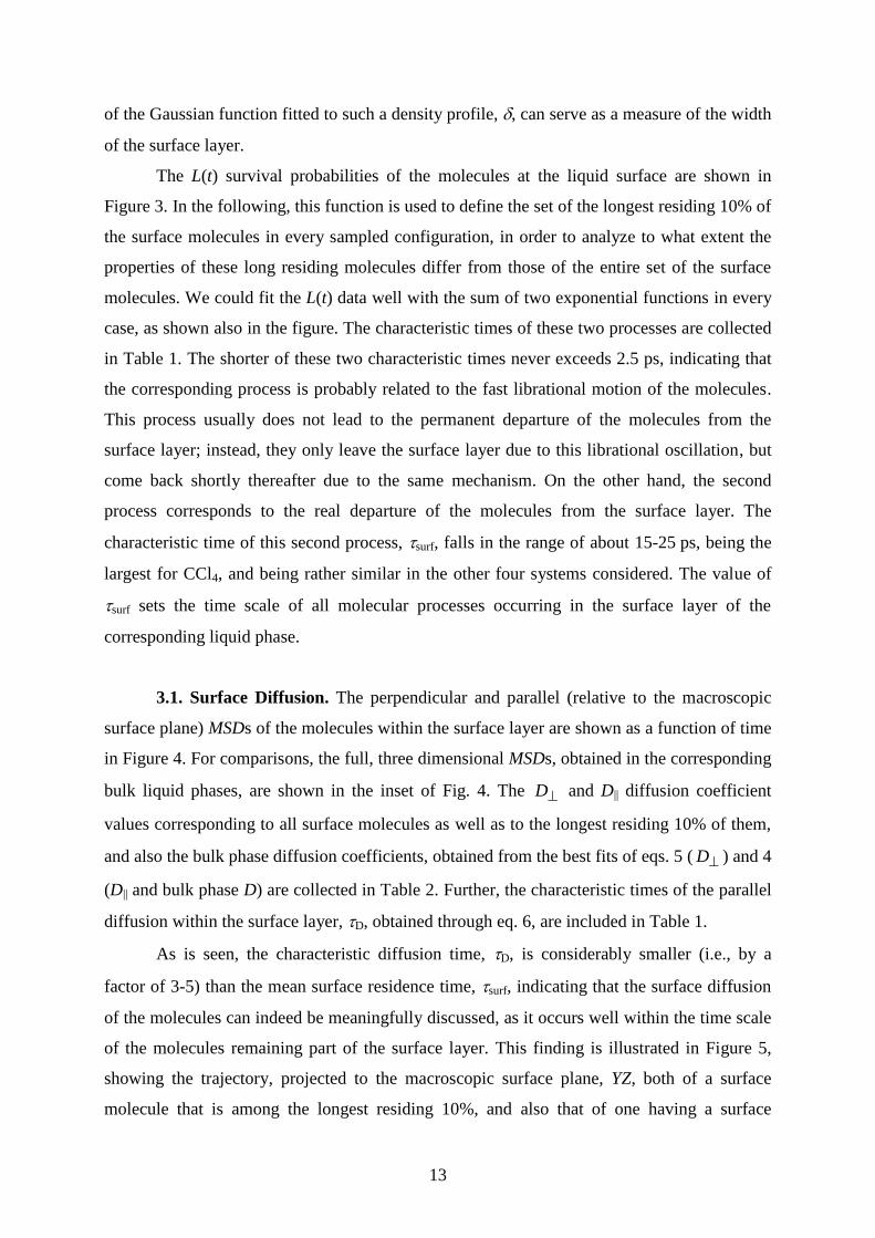
Besides the D value itself, the fitting of the perpendicular MSD data by eq. 5 also

yields the effective width of the surface layer, Leff. The values of Leff are collected in Table 3,

15

along with the width parameter of the surface layer density profiles, , as obtained for the five

liquids considered. As is seen, these values indeed correlate well with each other, their ratio

falling between about 1.4 and 1.8 in every case. Integration of the Gaussian-shape density

profile of the surface molecules (Fig. 2) in the distance range of the width Leff around its

center reveals that Leff is representative of an effective width that includes 83-92% of the

surface molecules for the different system, as detailed in Table 3.

Figure 6 a and b show the MSD of the surface molecules along the macroscopic

surface normal axis, X, as a function of time on two different time scales, normalized by the

mean surface residence time, surf, and by the characteristic time of surface diffusion, D,

respectively. The obtained MSD deviates downwards from linearity not only on the real time

scale up to 25 ps, but also on the scale of the surface residence time of the molecules in every

case. More precisely, the simulated data points start deviating from linearity at around 20-

40% of surf. This finding demonstrates that although the molecules can seemingly freely

diffuse also along the macroscopic surface normal in a non-negligible fraction of their surface

lifetime, they start feeling the presence of the boundaries still well within their lifetime at the

liquid surface, surf. On the other hand, as seen from Fig. 6.b, the MSDs are indeed linear up to

D, i.e., within the characteristic time scale of the lateral surface diffusion. To interpret this

finding, however, we have to emphasize that D is the upper limit of the time range within

which the molecules can still have memory of their initial position (i.e., they might still not

exhibit an uncorrelated random walk). The observed linearity of the perpendicular MSD can

thus either be related to the fact that, within this time scale, the molecules do not feel yet the

constraint of being in the surface layer and diffuse freely along the macroscopic surface

normal, or it can also be an artifact of the limited time window. Further investigation of the

possible physical meaning of the observed linearity of MSD within this time scale can be done

by analyzing the velocity autocorrelation function of the surface molecules, which is

presented in a subsequent sub-section.

3.2. Spatial Correlation between Long-Residing Surface Molecules. The diffusion

of the molecules that stay at the liquid surface for unusually long times did not turn out to be

markedly different from that of the other surface molecules in any case. To further investigate

whether long surface residence times of certain molecules simply occur randomly, or they are

related to certain properties of these molecules, we investigate how strongly the positions of

these molecules are correlated with each other at the liquid surface. In other words, we

16

address the question whether long-residing surface molecules are distributed randomly at the

liquid surface, or they form relatively dense patches, leaving large empty spaces between

them. For this purpose, we have projected the centers of the longest residing 10% of the

surface molecules to the macroscopic plane of the surface, YZ, and have calculated the

Voronoi cells85-87

around each of these projections. If these projections are randomly

distributed, the area (A) of the Voronoi cells is expected to follow approximately a gamma

distribution88,89

)exp()( 1 AAaAP (10)

where and are free parameters, while a is a normalization factor. On the other hand, in the

case of correlated arrangement of these projections the P(A) distribution deviates from eq. 10,

exhibiting a long tail of exponential decay at the large area side of its peak.90

The P(A) Voronoi cell area distributions are shown in Figure 7 as obtained in the five

systems simulated, together with their best fits by eq. 10. The exponential decay of all these

data sets (transformed to a linear decrease by the use of a logarithmic scale) as well as the

deviation from eq. 10 is clearly seen from the figure in every case. This finding indicates that

the long-residing molecules are distributed in a correlated way at the liquid surface, i.e., they

prefer to stay in the vicinity of each other. It is also apparent that this correlation is the

weakest for the hydrogen bonding liquids, in particular, for water, and strongest for CCl4. The

observed correlated arrangement of the long residing surface molecules at the liquid surface is

illustrated also in Figure 8, showing the projections of the centers of these molecules to the

macroscopic plane of the surface, YZ, in an equilibrium snapshot of both the CCl4 and the

water system.

3.3. Hydrogen Bonding at the Intrinsic Liquid Surface. In this sub-section we

address the point how the properties of the hydrogen bonds are affected by the liquid surface

in the two H-bonding liquids considered, i.e., methanol and water. Also, to further study the

question how unusually long surface residence time is related to other properties of the

molecules, we compare the properties of the H-bonds of the longest residing 10% of the

surface molecules with those of all surface molecules.

The average lifetime of a hydrogen bond can be defined in a similar way as the mean

surface residence time. Thus, the survival probability of a H-bond, LHB(t), is the probability

that a H-bond existing at time t0 will persist up to the time t0+t. Again, the breaking of a H-

17

bond is a process of first order kinetics, hence, LHB(t) is a function of exponential decay.

Therefore, the mean H-bond lifetime, HB, can simply be estimated by fitting the function

exp(-t/HB) to the simulated LHB(t) data. Similarly to the survival probability at the liquid

surface, L(t), the short time part of LHB(t) can also deviate from the exponential decay; this

transient part of the LHB(t) data, covering the first 0.1-0.5 ps of the time range, has thus been

left out from the exponential fit (see Figure 9). The HB values corresponding to the H-bond

between two surface molecules, included also in Table 1, are typically an order of magnitude

smaller for both H-bonding liquids considered than the mean surface residence time of the

molecules. Therefore, the H-bonds formed specifically by surface molecules can be

distinguished from those involving also bulk phase molecules, and thus their properties can

indeed be meaningfully discussed. It should be noted that the average lifetime of a H-bond at

the liquid surface is considerably, i.e., 25-40%, shorter than in the bulk liquid phase for both

H-bonding liquids considered: the HB values obtained in the bulk liquid phase of methanol

and water have turned out to be 5.22 ps and 2.01 ps (the corresponding surface values being

3.22 ps and 1.54 ps), respectively. On the other hand, the surface residence time of the

molecules is not related to the lifetime of their H-bonds, as the HB values corresponding to

the H-bonds between two long-residing surface molecules are 3.28 ps in methanol and 1.52 ps

in water.

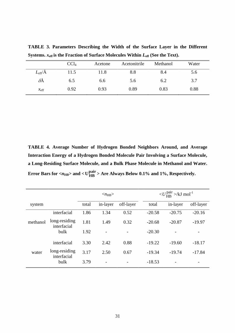
The average number of the H-bonds formed by a surface molecule, <nHB>, as well as

the average interaction energy of such a H-bonded molecule pair, <pairHBU >, are collected and

compared to the respective bulk phase values in Table 4. Values corresponding specifically to

the longest residing 10% of the surface molecules are also included in the table. Furthermore,

the <nHB> and <pairHBU > values corresponding to the interfacial molecules are also

decomposed according to the location of the H-bonding partner molecule (i.e., whether it also

belongs to the surface layer or not). As is clear from the data, the liquid surface does not have

a considerable influence on the H-bonding structure of the molecules in methanol. The

average number of the H-bonded neighbors of a surface methanol molecule is only 3% less

than that of a bulk phase one and, correspondingly, the interaction energy of such a molecule

pair agrees within 0.3 kJ/mol for molecule pairs being at the liquid surface and in the bulk

liquid phase. By contrast, interfacial water molecules have, on average, about 15% less H-

bonded neighbors than the bulk phase ones, while their pair interaction energy is, on average,

0.7 kJ/mol deeper than in the bulk liquid phase. This difference can be related to the preferred

18

surface orientations of these molecules. Namely, both of these molecules can easily be

oriented at the liquid surface in such a way that three of their tetrahedrally aligned H-bonding

(i.e., O-H and lone pair) directions are turned flatly towards the bulk liquid phase.13-15

Since

methanol molecules have only three H-bonding directions, they can efficiently maintain all of

their H-bonds even at the macroscopically flat liquid surface by sticking the fourth of the

tetrahedrally aligned electron pairs of their O atom (i.e., the O-CH3 bond) straight out to the

vapor phase.15

On the other hand, in water this fourth electron pair around the O atom also

represents a H-bonding direction. Therefore, alignments of the surface water molecules in

which three of the H-bonding directions are turned flatly inward involves the “sacrifice” of

the fourth of these directions, which is then turned straight towards the vapor phase.13,14

All

four H-bonding directions can only be turned towards the bulk liquid phase at strongly curved

portions of the liquid surface,13,14,91

such as at the tips of the ripples of the molecularly wavy

surface.

The energy loss corresponding to the fewer number of H-bonding neighbors is partly

compensated by a certain ordering of the H-bonding arrangement of the water molecules at

the liquid surface, which results, on average, in somewhat stronger H-bonds at the surface

than in the bulk phase (see Table 4). The observed small, about 4% strengthening of the H-

bonds at the surface of water is also in accordance with earlier results.82,92,93

It is interesting to

note that although the bulk phase H-bonds are, on average, slightly weaker in water, and are

about the same strength in methanol than the interfacial ones, H-bonds live considerably

longer in the bulk phase than at the interface of both liquids This finding is again in

accordance with earlier claims that the strength and lifetime of the H-bonds are independent

from each other.93,94

Instead of their strength, the shorter lifetime of the surface H-bonds can

be explained by the enhanced mobility of the surface molecules, as compared to that of the

bulk phase ones (see Table 2), due to their lack of attractive interactions at the vapor side of

the interface.

When comparing the properties of the long-residing molecules with those of all the

surface molecules, it is seen that long residing molecules form, on average, slightly, by 3-4%

less H-bonds than all the surface molecules. When decomposing these numbers into the

values corresponding to in-layer and off-layer H-bonds, it turns out that the average number

of H-bonding neighbors of the long residing surface molecules within the surface layer is

somewhat (i.e., by 11% in methanol and 3% in water) larger, while that of their non-surface

H-bonding neighbors is considerably (i.e., 38% in methanol and 25% in water) smaller than

the values corresponding to all surface molecules. The observed increase of the number of in-

19

layer H-bonds is in accordance with our previous finding that long residing molecules prefer

to stay in the vicinity of each other. However, the most striking feature of the long residing

surface molecules is clearly that they form much less hydrogen bonds with the subsurface

molecules than the value corresponding to all of the surface molecules. This fact can also

explain their long stay in the surface layer. Namely, having less off-layer H-bonded

neighbors, these molecules are better separated from the subsurface region, and hence can not

leave the surface as easily as the other ones.

3.4. Velocity Autocorrelation Function at the Intrinsic Liquid Surface. In Figure

10 we report the autocorrelation function of the in-plane molecular center of mass velocity for

the molecules belonging to the first layer, ||(t), and, for comparison, also the autocorrelation

function (t) of the molecular center of mass velocity in the corresponding bulk liquid

phases. The common trait, shared by all systems, is that the in-plane velocity of surface

molecules is always more correlated during the initial, rapid decay, which takes place within

the first 0.1-0.3 ps. Of all considered liquids, only CCl4 and acetone show, in the bulk, no

presence of the cage effect, and (t) is always positive, whereas ||(t) is considerably larger

at all times, with values clearly different from zero, also for time lags where (t) has already

vanished. In the case of acetonitrile, the two autocorrelation functions are different both

qualitatively and quantitatively from each other, as the negative part of (t) is not present any

more in ||(t). The latter function decays smoothly, resembling a memoryless process. In both

methanol and water the two autocorrelation functions share some common features, namely

an oscillation at 0.25 and 0.13 ps, respectively, which is the signature of hydrogen bonding.95

In methanol, however, the in-plane correlation function of the surface molecules is, again,

always positive, and the cage effect, which characterizes the bulk phase dynamics, is not

present within the surface layer. While methanol molecules retain the majority of their

hydrogen bonds at the liquid surface, the outward pointing arrangement of the CH3 groups at

the surface results in a much less crowded environment of the molecules. As a consequence,

the cage effect disappears, in accordance with the strongly enhanced surface diffusion

discussed previously. Water is the only case in which the in-plane correlation of the surface

molecules becomes negative, showing that the hydrogen bond network is strong enough to

influence the dynamics of the water molecules even within the surface layer. Our results

suggest that water behaves in a rather unique way in this respect, as no such behavior is seen

for the other liquids considered. Still, the in-plane velocity correlation of the surface

20

molecules is always larger than its bulk counterpart in the region of positive values, and

smaller in that of negative ones, showing therefore a larger mobility of the molecules, and a

less pronounced cage effect, which again explains the larger diffusion coefficient in the

surface, with respect to that in the bulk. This effect is, however, less pronounced here than in

the case of methanol, where caging is completely eliminated at the liquid surface.

4. Summary and Conclusions

In this paper, we have analyzed the single particle dynamical properties of the

molecules in the first molecular layer of five molecular liquids, ranging from apolar through

aprotic dipolar to hydrogen bonding ones. Such an analysis is clearly enabled by performing

an intrinsic analysis of the liquid surface. The analysis of the molecular residence times in the

first layer has shown that the dynamics of escape from the first layer is dictated by two

characteristic time scales. The first, fast process of escape takes place on the time scale of

about 2 ps for all liquids considered here, and is most likely representative of molecules

leaving the layer for short times due to librational motions. The other process dominates after

the first few picoseconds and takes place on the much longer scale of 15-25 ps, and is found

to be considerably larger than the characteristic time of in-layer diffusion and hydrogen bond

lifetime (for methanol and water), which are therefore meaningful observables for this set of

molecular liquids and thermodynamic points. We investigated the diffusion in the first layer

by sampling both the mean square displacement and the velocity autocorrelation function of

the molecular centers of mass. The mean square displacement parallel to the macroscopic

plane of the interface and perpendicular to it shows two qualitatively different behaviors,

namely, the common Einstein linear dependence of bulk systems (for the parallel diffusion),

and saturation behavior that fits extremely well with the diffusion between two reflecting

walls.56,78

The diffusion coefficients estimated from these two separate fits are markedly

different from the diffusion coefficient obtained in the bulk liquid phase, showing, in all

cases, a much (i.e., typically 3-4 times) larger surface diffusion with respect to the bulk. The

analysis of the in-plane velocity autocorrelation function confirmed this finding, showing that,

at the picosecond scale, molecules at the surface are in all cases more free to move than in the

bulk. At the surface, excluding the case of water, no trace of the cage effect is found, if this

was present in the bulk. In those cases, which did not present a cage effect even in the bulk

liquid phase (i.e., CCl4 and acetone), sizeable correlation with the initial velocity is found at

time lags, where the bulk counterpart shows no correlation any more. The analysis of the

21

spatial distribution of the long-residing surface molecules has revealed that they are clearly

characterized by some degree of clustering. The analysis of the hydrogen bonded neighbors

has shown that, in contrast to water, methanol is retaining practically all of its hydrogen

bonded neighbors at the liquid surface. This result might be surprising in the light of the much

higher diffusion coefficient of the methanol molecules found at the liquid surface than in the

bulk liquid phase, however, it is consistent with the pronounced tendency of methanol to

expose the bulky CH3 group to the vapor side of the interface,15

which also helps eliminating

the cage effect. This shows that the main factor in building up the internal friction for bulk

methanol is, in fact, presence of the CH3 groups rather than that of the hydrogen bonds

(which, unlike in liquid water, do not form a percolating network in bulk methanol66

). The

opposite happens in water, where the dynamics of the molecules is almost completely

dominated by the hydrogen bond networking, both in the bulk liquid phase and at its surface,

resulting also in its very high surface tension, with respect to all other molecular liquids

considered here.

In conclusion, the analysis of single particle dynamical properties at the intrinsic liquid

surface has proven to be very informative on the microscopic dynamics at liquid/vapor

interfaces, showing that mass transport properties are markedly different at the surface, with

respect to the bulk. In fact, these difference are surprising, considering the fact that, from the

structural point of view, the first molecular layer is not so much different (e.g., in terms of

density or hydrogen bonded neighbors) from the subsequent ones. The two- to fourfold

increase in mobility at the surface draws a picture of a much more fluid surface layer, sharing

some traits with those of rarefied fluids in case of non-hydrogen bonding liquids, which can

have important implication for diffusion-limited reactions occurring at interfaces.

Acknowledgements. This work has been supported by the Hungarian NKFIH

Foundation under Project Nos. 120075 and 119732, and by the Action Austria-Hungary

Foundation under project No. 93öu3. The calculations have been performed using the

computing resources of the ésocentre de Calcul, a regional computing center at niversité

de Franche-Comté.

22

References

(1) Shen, Y. R. The Principles of Nonlinear Optics, Wiley-Interscience: New York, 1984.

(2) Franken, P.; Hill, A.; Peters, C.; Weinreich, G. Generation of Optical Harmonics.

Phys. Rev. Letters 1961, 7, 118-120.

(3) Bloembergen, N.; Pershan, P. S. Light Waves at Boundary of Nonlinear Media. Phys.

Rev. 1962, 128, 606-623.

(4) Eisenthal, K. B. Liquid Interfaces Probed by Second-Harmonic and Sum-Frequency

Spectroscopy. Chem. Rev. 1996, 96, 1343–1360.

(5) Shen, Y. R. Surface Properties Probed by Second-Harmonic and Sum-Frequency

Generation. Nature, 1989, 337, 519-525.

(6) Richmond, G. L. Molecular Bonding and Interactions at Aqueous Surfaces as Probed

by Vibrational Sum Frequency Spectroscopy. Chem. Rev. 2002, 102, 2693-2724.

(7) Daillant, J.; Gibaud, A. X-Ray and Neutron Reflectivity: Principles and Applications,

Springer: Berlin, 1999.

(8) Tolan, M.; X-Ray Scattering from Soft-Matter Thin Films, Springer: Berlin, 1999.

(9) Penfold, J. Neutron Reflectivity and Soft Condensed Matter. Curr. Opin. Colloid

Interface Sci. 2002, 7, 139-147.

(10) Jähnig, F., Structural Order of Lipids and Proteins in Membranes: Evaluation of

Fluorescence Anisotropy Data. Proc. Natl. Acad. Sci. USA 1979, 76, 6361-6365.

(11) Cross, A. J.; Fleming, G. R. Analysis of Time-Resolved Fluorescence Anisotropy

Decays. Biophys. J. 1984, 46, 45-56.

(12) Allen, M. P.; Tildesley, D. J. Computer Simulation of Liquids; Clarendon Press:

Oxford, 1987.

(13) Pártay, L. B.; Hantal, Gy.; Jedlovszky, P.; Vincze, Á.; Horvai, G. A New Method for

Determining the Interfacial Molecules and Characterizing the Surface Roughness in

Computer Simulations. Application to the Liquid–Vapor Interface of Water. J. Comp.

Chem. 2008, 29, 945-956.

(14) Hantal, Gy.; Darvas, .; Pártay, L. B.; Horvai, G.; Jedlovszky, P. Molecular Level

Properties of the Free Water Surface and Different Organic Liquid/Water Interfaces,

As Seen from ITIM Analysis of Computer Simulation Results. J. Phys.: Condens.

Matter 2010, 22, 284112-1-14.

23

(15) Pártay, L. B.; Jedlovszky, P.; Vincze, Á.; Horvai, G. Properties of Free Surface of

Water-Methanol Mixtures. Analysis of the Truly Interfacial Molecular Layer in

Computer Simulation. J. Phys. Chem. B. 2008, 112, 5428-5438.

(16) Pártay, L. B.; Jedlovszky, P.; Horvai, G. Structure of the Liquid-Vapor Interface of

Water-Acetonitrile Mixtures As Seen from Molecular Dynamics Simulations and

Identification of Truly Interfacial Molecules Analysis. J. Phys. Chem. C. 2009, 113,

18173-18183.

(17) Fábián, B.; Szőri, .; Jedlovszky, P. Floating Patches of HCN at the Surface of Their

Aqueous Solutions – Can They ake “HCN World” Plausible? J. Phys. Chem. C

2014, 118, 21469-21482.

(18) Pártay, L. B.; Horvai, G.; Jedlovszky, P. Temperature and Pressure Dependence of the

Properties of the Liquid-Liquid Interface. A Computer Simulation and Identification

of the Truly Interfacial Molecules Investigation of the Water-Benzene System. J.

Phys. Chem. C. 2010, 114, 21681-21693.

(19) Linse, P. Monte Carlo Simulation of Liquid-Liquid Benzene-Water Interface. J. Chem.

Phys. 1987, 86, 4177-4187.

(20) Benjamin, I. Theoretical Study of the Water/1,2-Dichloroethane Interface: Structure,

Dynamics, and Conformational Equilibria at the Liquid-Liquid Interface. J. Chem.

Phys. 1992, 97, 1432-1445.

(21) Chacón, E.; Tarazona, P. Intrinsic Profiles Beyond the Capillary Wave Theory: A

Monte Carlo Study. Phys Rev. Letters 2003, 91, 166103-1-4.

(22) Chacón, E.; Tarazona, P. Characterization of the Intrinsic Density Profiles for Liquid

Surfaces. J. Phys.: Condens. Matter 2005, 17, S3493-S3498.

(23) Tarazona, P.; Chacón, E. onte Carlo Intrinsic Surfaces and Density Profiles for

Liquid Surfaces. Phys. Rev. B 2004, 70, 235407-1-13.

(24) Jorge, M.; Cordeiro, M. N. D. S. Intrinsic Structure and Dynamics of the

Water/Nitrobenzene Interface. J. Phys. Chem. C. 2007, 111, 17612-17626.

(25) Jorge, M.; Cordeiro, M. N. D. S. Molecular Dynamics Study of the Interface between

Water and 2-Nitrophenyl Octyl Ether. J. Phys. Chem. B 2008, 112, 2415-2429.

(26) Chowdhary, J.; Ladanyi, B. M. Water-Hydrocarbon Interfaces: Effect of Hydrocarbon

Branching on Interfacial Structure. J. Phys. Chem. B. 2006, 110, 15442-15453.

(27) Jorge, M.; Jedlovszky, P.; Cordeiro, M. N. D. S. A Critical Assessment of Methods for

the Intrinsic Analysis of Liquid Interfaces. 1. Surface Site Distributions. J. Phys.

Chem. C. 2010, 114, 11169-11179.

24

(28) Mezei, M. A New Method for Mapping Macromolecular Topography. J. Mol.

Graphics Modell. 2003, 21, 463-472.

(29) Wilard, A. P.; Chandler, D. Instantaneous Liquid Interfaces. J. Phys. Chem. B. 2010,

114, 1954-1958.

(30) Sega, M.; Kantorovich, S.; Jedlovszky, P; Jorge, M. The Generalized Identification of

Truly Interfacial Molecules (ITIM) Algorithm for Nonplanar Interfaces. J. Chem.

Phys. 2013, 138, 044110-1-10.

(31) Jorge, M.; Hantal, G.; Jedlovszky, P.; Cordeiro, M. N. D. S. A Critical Assessment of

Methods for the Intrinsic Analysis of Liquid Interfaces: 2. Density Profiles. J. Phys.

Chem. C. 2010, 114, 18656-18663.

(32) Sega, M.; Fábián, B.; Jedlovszky, P. Layer-by-Layer and Intrinsic Analysis of

Molecular and Thermodynamic Properties across Soft Interfaces. J. Chem. Phys. 2015,

143, 114709-1-8.

(33) Darvas, M.; Jorge, M.; Cordeiro, M. N. D. S.; Kantorovich, S. S.; Sega, M.;

Jedlovszky, P. Calculation of the Intrinsic Solvation Free Energy Profile of an Ionic

Penetrant Across a Liquid/Liquid Interface with Computer Simulations. J. Phys.

Chem. B 2013, 117, 16148-16156.

(34) Darvas, M.; Jorge, M.; Cordeiro, M. N. D. S.; Jedlovszky, P. Calculation of the

Intrinsic Free Energy Profile of Methane Across a Liquid/Liquid Interface in

Computer Simulations. J. Mol. Liquids 2014, 189, 39-43.

(35) Bresme, F.; Chacón, E.; Tarazona, P.; Wynveen, A. The Structure of Ionic Aqueous

Solutions at Interfaces: An Intrinsic Structure Analysis. J. Chem. Phys. 2012, 137,

114706-1-10.

(36) Sega, .; Fábián, B.; Horvai, G.; Jedlovszky, P. How Is the Surface Tension of

Various Liquids Distributed along the Interface Normal? J. Phys. Chem. C 2016, 120,

27468-27477.

(37) Sega, M.; Horvai, G.; Jedlovszky, P. Microscopic Origin of the Surface Tension

Anomaly of Water. Langmuir 2014, 30, 2969-2972.

(38) Sega, M.; Horvai, G.; Jedlovszky, P. Two-Dimensional Percolation at the Free Water

Surface and its Relation with the Surface Tension Anomaly of Water. J. Chem. Phys.

2014, 141, 054707-1-11.

(39) Bresme, F.; Chacón, E.; artínez, H.; Tarazona, P. Adhesive Transitions in Newton

Black Films: A Computer Simulation Study. J. Chem. Phys. 2011, 134, 214701-1-12.

25

(40) Abrankó-Rideg, N.; Darvas, M.; Horvai, G.; Jedlovszky, P. Immersion Depth of

Surfactants at the Free Water Surface: A Computer Simulation and ITIM Analysis

Study. J. Phys. Chem. B 2013, 117, 8733-8746.

(41) Hantal, G.; Cordeiro, M. N. D. S.; Jorge, M. What Does an Ionic Liquid Surface

Really Look Like? Unprecedented Details from Molecular Simulations. Phys. Chem.

Chem. Phys. 2011, 13, 21230-21232.

(42) Lísal, .; Posel, Z.; Izák, P. Air–Liquid Interfaces of Imidazolium-Based [TF2N-]

Ionic Liquids: Insight from Molecular Dynamics Simulations. Phys. Chem. Chem.

Phys. 2012, 14, 5164-5177.

(43) Hantal, G.; Voroshylova, I.; Cordeiro, M. N. D. S.; Jorge, M. A Systematic Molecular

Simulation Study of Ionic Liquid Surfaces Using Intrinsic Analysis Methods. Phys.

Chem. Chem. Phys. 2012, 14, 5200-5213.

(44) Lísal, .; Izák, P. Molecular Dynamics Simulations of n-Hexane at 1-Butyl-3-

Methylimidazolium bis(Trifluoromethylsulfonyl) Imide Interface. J. Chem. Phys.

2013, 139, 014704-1-15.

(45) Hantal, G.; Sega, M.; Kantorovich, S.; Schröder, C.; Jorge, . Intrinsic Structure of

the Interface of Partially Miscible Fluids: An Application to Ionic Liquids. J. Phys.

Chem. C. 2015, 119, 28448-28461.

(46) Darvas, .; Pojják, K.; Horvai, G.; Jedlovszky, P. Molecular Dynamics Simulation

and Identification of the Truly Interfacial Molecules (ITIM) Analysis of the Liquid-

Vapor Interface of Dimethyl Sulfoxide. J. Chem. Phys. 2010, 132, 134701-1-10.

(47) Kiss, P.; Darvas, M.; Baranyai, A.; Jedlovszky, P. Surface Properties of the

Polarizable Baranyai-Kiss Water Model. J. Chem. Phys. 2012, 136, 114706-1-11.

(48) Jedlovszky, P.; Jójárt, B.; Horvai, G. Properties of the Intrinsic Surface of Liquid

Acetone, as Seen from Computer Simulations. Mol. Phys. 2015, 113, 985-996.

(49) Pojják, K.; Darvas, M.; Horvai, G.; Jedlovszky, P. Properties of the Liquid-Vapor

Interface of Water-Dimethyl Sulfoxide Mixtures. A Molecular Dynamics Simulation

and ITIM Analysis Study. J. Phys. Chem. C. 2010, 114, 12207-12220.

(50) Idrissi, A.; Hantal, G.; Jedlovszky, P. Properties of the Liquid-Vapor Interface of

Acetone-Methanol Mixtures, As Seen from Computer Simulation and ITIM Surface

Analysis. Phys. Chem. Chem. Phys. 2015, 17, 8913-8926.

(51) Fábián, B.; Jójárt, B.; Horvai, G.; Jedlovszky, P. Properties of the Liquid-Vapor

Interface of Acetone-Water Mixtures. A Computer Simulation and ITIM Analysis

Study. J. Phys. Chem. C. 2015, 119, 12473-12487.

26

(52) Lindahl, E; Edholm, O. Solvent Diffusion Outside Macromolecular Surfaces. Phys.

Rev. E 1998, 57, 791-796.

(53) Åman, K.; Lindahl, E.; Edholm, O.; Håkansson, P.; Westlund, P. O. Structure and

Dynamics of Interfacial Water in an L Phase Lipid Bilayer from Molecular Dynamics

Simulations. Biophys. J. 2003, 84, 102-115.

(54) Liu, P.; Harder, E.; Berne, B. On the Calculation of Diffusion Coefficientsin Confined

Fluids and Interfaces with an Application to the Liquid-Vapor Interface of Water. J.

Phys. Chem. B 2004, 108, 6595-6602.

(55) Bühn, J. B.; Bopp, P. A.; Hampe, . J. A olecular Dynamics Study of the Liquid-

Liquid Interface: Structure and Dynamics. Fluid Phase Equilib. 2004, 224, 221-230.

(56) Sega, M.; Vallauri, R.; Melchionna, S. Diffusion of Water in Confined Geometry: The

Case of a Multilamellar Bilayer. Phys. Rev. E 2005, 72, 041201-1-4.

(57) Bhide, S. Y.; Berkowitz, M. L. Structure and Dynamics of Water at the Interface with

Phospholipid Bilayers. J. Chem. Phys. 2005, 123, 224702-1-16.

(58) Benjamin, I. Reactivity and Dynamics at Liquid Interfaces. In: Reviews in

Computational Chemistry, Parrill, A. L.; Lipkowitz, K. B., Eds.; Wiley: Chichester,

2015; Vol. 28, pp. 205-313.

(59) Chowdhary, J.; Ladanyi, B. M. Water-Hydrocarbon Interfaces: Effect of Hydrocarbon

Branching on Single-Molecule Relaxation. J. Phys. Chem. B. 2008, 112, 6259-6273.

(60) Duque, D.; Tarazona, P.; Chacón, E. Diffusion at the Liquid-Vapor Interface. J. Chem.

Phys. 2008, 128, 134704-1-10.

(61) Delgado-Buscalioni, R.; Chacón, E.; Tarazona, P. Hydrodynamics of Nanoscopic

Capillary Waves. Phys. Rev. Letters 2008, 101, 106102-1-4.

(62) Delgado-Buscalioni, R.; Chacón, E.; Tarazona, P. Capillary Waves' Dynamics at the

Nanoscale, J. Phys.: Condens. Matter 2008, 20, 494229-1-6.

(63) Fábián, B.; Senćanski, . V.; Cvijetić, I. N.; Jedlovszky, P.; Horvai, G. Dynamics of

the Water Molecules at the Intrinsic Liquid Surface As Seen from Molecular

Dynamics Simulation and Identification of Truly Interfacial Molecules Analysis. J.

Phys. Chem. C. 2016, 120, 8578-8588.

(64) Geiger, A.; Stillinger, F. H.; Rahman, A. Aspects of the Percolation Process for

Hydrogen-Bond Networks in Water. J. Chem. Phys. 1979, 70, 4185-4193.

(65) Stanley, H. E.; Teixeira, J. Interpretation of the Unusual Behavior of H2O and D2O at

Low Temperatures. Test of a Percolation Model. J. Chem. Phys. 1980, 73, 3404-3422.

27

(66) Pálinkás, G.; Hawlicka, E.; Heinzinger, K. A olecular Dynamics Study of Liquid

Methanol with a Flexible Three-Site Model. J. Phys. Chem. 1987, 91, 4334-4341.

(67) Duffy, E. M.; Severance, D. L.; Jorgensen, W. L. Solvent Effects on the Barrier to

Isomerization for a Tertiary Amide from Ab Initio and Monte Carlo Calculations. J.

Am. Chem. Soc. 1992, 114, 7535–7542.

(68) Stubbs, J. M.; Potoff, J. J.; Siepmann, J. I. Transferable Potentials for Phase

Equilibria. 6. United-Atom Description for Ethers, Glycols, Ketones, and Aldehydes.

J. Phys. Chem. B 2004, 108, 17596-17605.

(69) Berendsen, H. J. C.; Grigera, J. R.; Straatsma, T. The Missing Term in Effective Pair

Potentials. J. Phys. Chem. 1987, 91, 6269-6271.

(70) Böhm, H. J.; cDonald, I. R.; adden, P. A. An Effective Pair Potential for Liquid

Acetonitrile. Mol. Phys. 1983, 49, 347-360.

(71) Walser, R.; Mark, A. E.; van Gunsteren, W. F.; Lauterbach , M.; Wipff, G. The Effect

of Force-Field Parameters on Properties of Liquids: Parametrization of a Simple

Three-Site Model for Methanol. J. Chem. Phys. 2000, 112, 10450-10459.

(72) Ryckaert, J. P.; Ciccotti, G.; Berendsen, H. J. C. Numerical Integration of the

Cartesian Equations of Motion of a System With Constraints; Molecular Dynamics of

n-Alkanes. J. Comp. Phys. 1977, 23, 327–341.

(73) Essman, U.; Perera, L.; Berkowitz, M. L.; Darden, T.; Lee, H.; Pedersen, L. G. A

Smooth Particle Mesh Ewald Method. J. Chem. Phys. 1995, 103, 8577-8594.

(74) Pronk, S.; Páll, S.; Schulz, R.; Larsson, P.; Bjelkmar, P.; Apostolov, R.; Shirts, . R.;

Smith, J. C.; Kasson, P. M.; van der Spoel; D., et al. GROMACS 4.5: A High-

Throughput and Highly Parallel Open Source Molecular Simulation Toolkit.

Bioinformatics 2013, 29, 845–854.

(75) Nosé, S. A olecular Dynamics ethod for Simulations in the Canonical Ensemble.

Mol. Phys. 1984, 52, 255-268.

(76) Hoover, W. G. Canonical Dynamics: Equilibrium Phase-Space Distributions. Phys.

Rev. A 1985, 31, 1695-1697.

(77) Sega, M. The Role of a Small-Scale Cutoff in Determining Molecular Layers at Fluid

Interfaces. Phys. Chem. Chem. Phys. 2016, 18, 23354-23357.

(78) Lindahl, E.; Edholm, O. Solvent Diffusion Outside Macromolecular Surfaces. Phys.

Rev E 1998, 57, 791-796.

28

(79) Rideg, N. A.; Darvas, M.; Varga, I.; Jedlovszky, P. Lateral Dynamics of Surfactants at

the Free Water Surface. A Computer Simulation Study. Langmuir 2012, 28, 14944-

14953.

(80) Chowdhary, J.; Ladanyi, B. M. Surface Fluctuations at the Liquid-Liquid Interface.

Phys. Rev. E 2008, 77, 031609-1-14.

(81) Jedlovszky, P. The Hydrogen Bonding Structure of Water at the Vicinity of Apolar

Interfaces. A Computer Simulation Study. J. Phys.: Condens. Matter 2004, 16, S5389-

S5402.

(82) Wakisaka, A.; Abdoul-Carime, H.; Yamamoto, Y.; Kiyozumi, Y. Non-Ideality of

Binary Mixtures Water-Methanol and Water-Acetonitrile from the Viewpoint of

Clustering Structure. J. Chem. Soc. Faraday Trans. 1998, 94, 369-374.

(83) Dixit, S.; Crain, J.; Poon, W. C. K.; Finney, J. L.; Soper, A. K. Molecular Segregation

Observed in a Concentrated Alcohol-Water Solution. Nature 2002, 416, 829-832.

(84) Dougan, L.; Bates, S. P.; Hargreaves, R.; Fox, J. P.; Crain, J.; Finney, J. L.; Réat, V.;

Soper, A. K. Methanol-Water Solutions: A Bi-Percolating Liquid Mixture. J. Chem.

Phys. 2004, 121, 6456-62.

(85) Voronoi, G. F. Recherches sur le Paralléloèders Primitives. J. Reine Angew. Math.

1908, 134, 198-287.

(86) Okabe, A.; Boots, B.; Sugihara, K.; Chiu, S. N. Spatial Tessellations: Concepts and

Applications of Voronoi Diagrams, John Wiley: Chichester, 2000.

(87) Medvedev, N. N. The Voronoi-Delaunay Method in the Structural Investigation of

Non-Crystalline Systems, SB RAS: Novosibirsk, 2000, in Russian.

(88) Kiang, T. Random Fragmentation in Two and Three Dimensions. Z. Astrophys. 1966,

63, 433-439.

(89) Pineda, E.; Bruna, P.; Crespo, D. Cell Size Distribution in Random Tessellations of

Space. Phys. Rew. E. 2004, 70, 066119-1-8.

(90) Zaninetti, L. The Voronoi Tessellation Generated from Different Distributions of

Seeds. Phys. Letters A 1992, 165, 143-147.

(91) Jedlovszky, P.; Předota, .; Nezbeda, I. Hydration of Apolar Solutes of Varying Size:

A Systematic Study. Mol. Phys. 2006, 104, 2465-2476.

(92) Nihonyanagi, S.; Ishiyama, T.; Lee, T. K.; Yamaguchi, S.; Bonn, M.; Morita, A.;

Tahara, T. Unified Molecular View of the Air/Water Interface Based on Experimental

and Theoretical (2)

Spectra of an Isotopically Diluted Water Surface. J. Am. Chem.

Soc. 2011, 133, 16875-16880.

29

(93) Vila Verde, A.; Bolhuis, P. G.; Campen, R. K. Statics and Dynamics of Free and

Hydrogen Bonded OH Groups at the Air/Water Interface. J. Phys. Chem. B. 2012,

116, 9467-9481.

(94) Laage, D.; Hynes, J. T. Do More Strongly Hydrogen-Bonded Water Molecules

Reorient More Slowly? Chem. Phys. Letters 2006, 433, 80-85.

(95) Balucani, U.; Brodholt, J. P.; Vallauri, R, Analysis of the Velocity Autocorrelation

Function of Water. J. Phys.: Condens. Matter 1996, 8, 6139-6144.

30

Tables

TABLE 1. Characteristic Times of Various Molecular Processes Occurring in the

Surface Layer of the Liquids Studied (in ps Units). Values in Parenthesis Correspond to

the Initial, Fastly Decaying Process of Leaving the Liquid Surface. Error Bars Are

Always Below 1%. The Dipole Moment of the Molecular Models Used () Is Also

Included in the Table.

system surf D HB /D

CCl4 26.2 (2.5) 7.20 - 0.00

Acetone 16.1 (2.0) 2.97 - 2.50

Acetonitrile 14.5 (1.8) 3.39 - 4.14

Methanol 16.4 (2.0) 4.34 2.27 2.28

Water 15.0 (1.7) 4.11 1.36 2.35

TABLE 2. Diffusion Coefficients within the Surface Layer (in Å2/ps Units), Both Along

with and Perpendicular to the Macroscopic Plane of the Surface, and Inside the Bulk

Liquid Phase of the Systems Studied. Values in Parenthesis Correspond to the Longest

Residing 10% of the Surface Molecules. Error bars Are Always Below 3%.

CCl4 Acetone Acetonitrile Methanol Water

Surface D 0.70 (0.73) 1.52 (1.66) 1.09 (1.18) 0.74 (0.76) 0.51 (0.51)

D|| 0.99 (1.03) 2.04 (2.19) 1.46 (1.56) 0.74 (0.76) 0.52 (0.53)

Bulk D 0.24 0.55 0.42 0.28 0.27

31

TABLE 3. Parameters Describing the Width of the Surface Layer in the Different

Systems. xeff is the Fraction of Surface Molecules Within Leff (See the Text).

CCl4 Acetone Acetonitrile Methanol Water

Leff/Å 11.5 11.8 8.8 8.4 5.6

Å 6.5 6.6 5.6 6.2 3.7

xeff 0.92 0.93 0.89 0.83 0.88

TABLE 4. Average Number of Hydrogen Bonded Neighbors Around, and Average

Interaction Energy of a Hydrogen Bonded Molecule Pair Involving a Surface Molecule,

a Long-Residing Surface Molecule, and a Bulk Phase Molecule in Methanol and Water.

Error Bars for <nHB> and <pairHB

U > Are Always Below 0.1% and 1%, Respectively.

<nHB> <pairHBU >/kJ mol

-1

system total in-layer off-layer total in-layer off-layer

methanol

interfacial 1.86 1.34 0.52 -20.58 -20.75 -20.16

long-residing

interfacial 1.81 1.49 0.32 -20.68 -20.87 -19.97

bulk 1.92 - - -20.30 - -

water

interfacial 3.30 2.42 0.88 -19.22 -19.60 -18.17

long-residing

interfacial 3.17 2.50 0.67 -19.34 -19.74 -17.84

bulk 3.79 - - -18.53 - -

32

Figure legend

Figure 1. Equilibrium snapshot of the surface portion of the five systems simulated.

Molecules belonging to the surface layer are shown enlarged. C, Cl, O, N, and H atoms are

marked by light blue, green, red, dark blue, and white color, respectively.

Figure 2. Molecular number density profile of the five systems simulated (dashed lines) and

those of their surface layer (open circles) along the macroscopic surface normal axis, X. The

Gaussian functions fitted to the surface layer profiles are shown by solid lines. All profiles

shown are symmetrized over the two liquid-vapor interfaces present in the basic box. CCl4:

black, acetone: red, acetonitrile: orange, methanol: blue, water: green.

Figure 3. Survival probability of the molecules within the surface layer of their liquid phase,

shown on a semi-logarithmic scale, as obtained in the five systems simulated (full circles).

The sums of the two exponentially decaying functions, fitted to these data sets, are shown by

solid lines. Color coding of the systems is the same as in Fig. 2.

Figure 4. Mean square displacements of the surface molecules along the macroscopic surface

normal axis, X (top panel), and within the macroscopic plane of the surface, YZ (bottom

panel) as a function of time, as obtained in the five systems simulated. The inset shows the

MSD vs. t data obtained in the bulk liquid phase of these liquids. Fits of the one dimensional

MSD vs. t data by eq 5 as well as linear fits of the two and three dimensional data are shown

by solid lines. Color coding of the systems is the same as in Fig. 2.

Figure 5. Trajectory of a surface molecule that belongs to the longest residing 10% at the

liquid surface (open circles), and of a surface molecule the surface residence time of which

roughly equals to its mean value (full circles), projected to the macroscopic plane of the

surface, YZ, as taken out from all five systems simulated. Color coding of the systems is the

same as in Fig. 2.

33

Figure 6. One dimensional mean square displacement of the molecules belonging to the

surface layer along the macroscopic surface normal axis, X, as obtained in the five systems

simulated, shown on the time scales corresponding to the characteristic times of (a) the

surface residence time, and (b) the lateral diffusion of the surface molecules. Color coding of

the systems is the same as in Fig. 2.

Figure 7. Distribution of the area of the Voronoi cells of the projections of the surface

molecules onto the macroscopic plane of the surface, YZ as obtained in the five systems

simulated. To emphasize the exponential decay of the distributions at large area values, the

data are shown on a semi-logarithmic scale. Best fits of the data by eq. 10 are shown by solid

lines. Color coding of the systems is the same as in Fig. 2.

Figure 8. Equilibrium snapshot of the liquid surface of CCl4 (left) and water (right) from the

top view, showing the projection of the centers of the longest residing 10% of the surface

molecules to the macroscopic plane of the surface, YZ.

Figure 9. Survival probability of the hydrogen bonds formed by two molecules at the liquid

surface (full circles), two long-residing surface molecules (open circles), and two molecules

in the bulk liquid phase (asterisks), as obtained in methanol (blue) and water (green). To

emphasize their exponential decay, the data are shown on a semi-logarithmic scale. The

exponentially decaying functions fitted to the long time part of the data are shown by solid

lines.

Figure 10. Normalized velocity autocorrelation function of the centers of mass of the surface

molecules in the macroscopic plane of the surface, YZ (solid lines), and that of the three

dimensional velocity of the molecules in the bulk liquid phase (dashed lines) of the five

molecular systems studied. The insets show the relevant part of the functions on an enlarged

scale. Color coding of the systems is the same as in Fig. 2.

34

Figure 1.

Fábián et al.

CCl4

Acetone

Acetonitrile

Methanol

Water

35

Figure 2.

Fábián et al.

0 25 50 75 100 125 150 1750.00

0.01

0.02

0.03 CCl4, entire system

CCl4, surface layer

Acetone, entire system

Acetone, surface layer

Acetonitrile, entire system

Acetonitrile, surface layer

Methanol, entire system

Methanol, surface layer

Water, entire system

Water, surface layer

/ Å

-3

X / Å

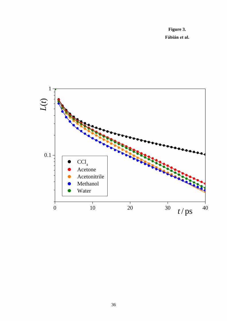
36

Figure 3.

Fábián et al.

0 10 20 30 40

0.1

1

CCl4

Acetone

Acetonitrile

Methanol

Water

L(t

)

t / ps

37

Figure 4.

Fábián et al.

0

5

10

15

20

25

0 5 10 15 20 250

50

100

150

200

0 5 10 15 20 250

20

40

60

80

parallel

CCl4

Acetone

Acetonitrile

Methanol

Water

perpendicular

M

SD

/ Å2

bulk

t / ps

MSD

/Å2

t/ps

38

Figure 5.

Fábián et al.

-20 -10 0 10 20

-20

-10

0

10

20

acetonitrile

acetone

acetonemethanol

water

water

CCl4

CCl4

Z/Å

Y/Å

39

Figure 6.

Fábián et al.

(a)

(b)

0.0 0.2 0.4 0.6 0.8 1.00

2

4

6

8

MSD

/ Å2

t/D

CCl4

Acetone

Acetonitrile

Methanol

Water

0.0 0.2 0.4 0.6 0.8 1.00

5

10

15

MSD

/ Å2

t/surf

CCl4

Acetone

Acetonitrile

Methanol

Water

40

Figure 7.

Fábián et al.

0 250 500 750 1000

1E-5

1E-4

1E-3

0.01

0.1

P(A

)

A/Å2

CCl4

Acetone

Acetonitrile

Methanol

Water

41

Figure 8.

Fábián et al.

-20 -10 0 10 20

-20

-10

0

10

20

-20 -10 0 10 20

-20

-10

0

10

20

waterCCl4

X/Å

Y/Å

X/Å

Y/Å

42

Figure 9.

Fábián et al.

0 1 2 3 4 5 6

0.01

0.1

1

LH

B(t

)

t/ps

methanol, surface

methanol, long residing

methanol, bulk

water, surface

water, long-residing

water, bulk

43

Figure 10.

Fábián et al.

0.0 0.1 0.2 0.3 0.4 0.5 0.6

0.00

0.25

0.50

0.75

1.000.00

0.25

0.50

0.75

1.000.00

0.25

0.50

0.75

1.000.00

0.25

0.50

0.75

1.000.00

0.25

0.50

0.75

1.00

0.1 0.2 0.3 0.4 0.5-0.1

0.0

0.1

0.2

0.1 0.2 0.3 0.4 0.5 0.6-0.1

0.0

0.1

0.2

0.2 0.3 0.4 0.5 0.6-0.1

0.0

0.1

0.2

Water

(t

)/

(0)

||(t)/

||(0)

t/ps

Methanol

Acetonitrile

Acetone

CCl4

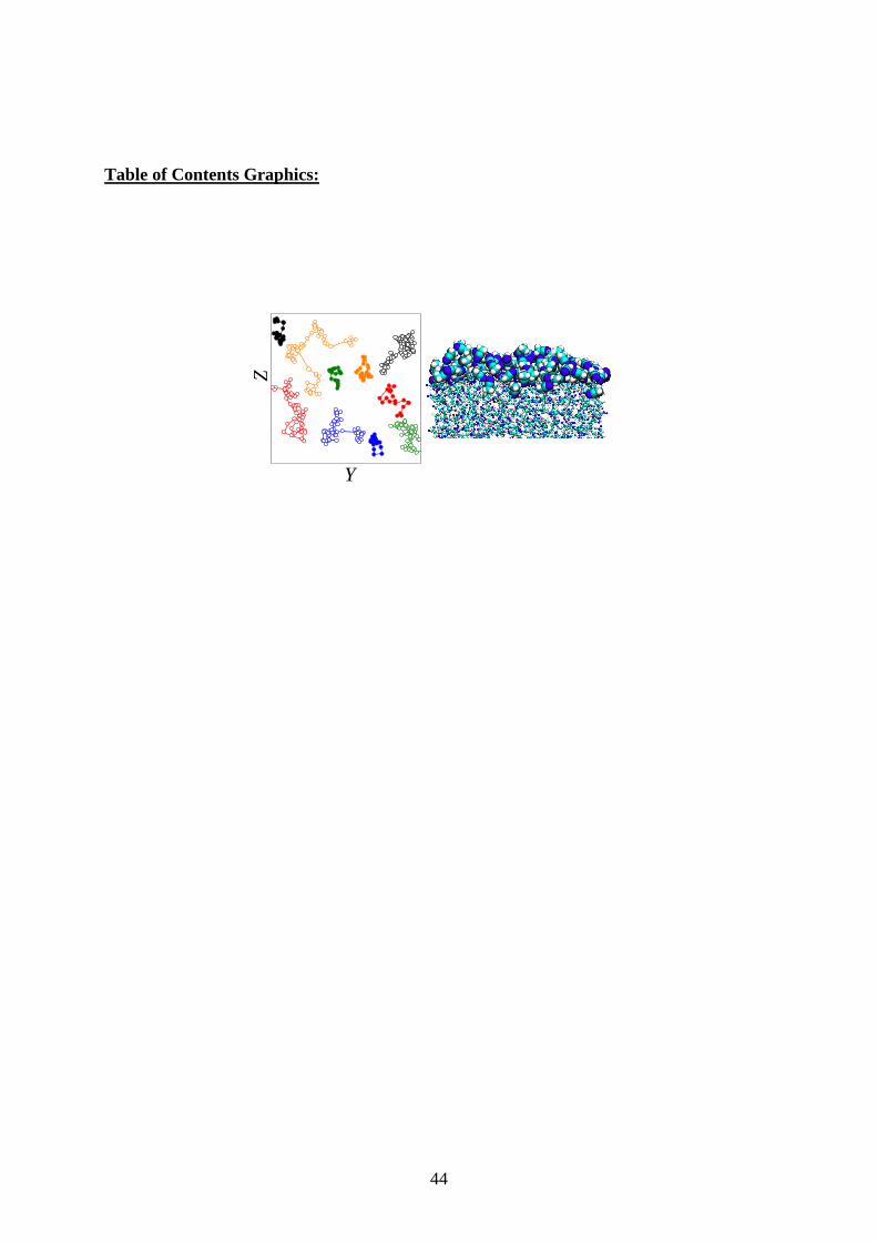
44

Table of Contents Graphics:

Z

Y