do federal grants boost school spending? evidence...
TRANSCRIPT
www.elsevier.com/locate/econbase
Journal of Public Economics 88 (2004) 1771–1792
Do federal grants boost school spending?
Evidence from Title I
Nora Gordon
Department of Economics, University of California, San Diego, CA 92093 0508, USA
Received 6 April 2003; received in revised form 5 August 2003; accepted 17 September 2003
Abstract
One of the federal government’s main elementary and secondary education programs is Title I,
which allocates money for compensatory education to school districts based on child poverty. I use
sharp changes in per-pupil grant amounts surrounding the release of decennial census data to identify
effects of Title I on state and local education revenue, and how much the program ultimately
increases spending by recipient school districts. I find that state and local revenue efforts initially are
unaffected by Title I changes, but that local governments substantially and significantly crowd out
changes in Title I within in a 3-year period.
D 2003 Elsevier B.V. All rights reserved.
JEL classification: H7; H4; I2
Keywords: Fiscal federalism; Intergovernmental grants; Education finance; Compensatory education
1. Introduction
Title I is widely recognized as the federal government’s single most important
education program. It attempts to increase the resources of school districts that serve
economically disadvantaged children, and cost $10.4 billion in FY 2002. It thus
represents one-third of the US Department of Education’s elementary and secondary
budget. The program makes non-matching grants to school districts based on their
number of poor children, and specifies that the grants be used so that educationally
disadvantaged children receive compensatory education, such as small group instruction
outside the classroom. Not only has Title I traditionally been the main way the federal
government directly aids poor local schools, but among the 10% of school districts that
0047-2727/$ - see front matter D 2003 Elsevier B.V. All rights reserved.
doi:10.1016/j.jpubeco.2003.09.002
E-mail address: [email protected] (N. Gordon).
N. Gordon / Journal of Public Economics 88 (2004) 1771–17921772
rely most heavily on the program, Title I accounts for between 5% and 10% of total
spending. Under the No Child Left Behind Act of 2001 (NCLB), the Title I program has
taken on a new accountability role as well: schools designated as in need of
improvement may lose Title I funds.1
If other revenue sources to school districts systematically offset gains from Title I, the
program will have less than its intended effect on the schooling experienced by poor
children. School districts’ budgets are determined by as many as three levels of
government, in addition to the federal government: states, local governments such as
counties and municipalities, and school districts. Any of these other levels of government
could potentially offset Title I revenue. If this is the case, federal dollars subsidize other
levels of government rather than supplement instructional resources for poor children. In
this paper, I estimate the effect of Title I on school spending, and examine how local and
state governments respond to changes in the federal program.
One of this paper’s benefits is that it will begin to untangle some of the controversy
about the effects of Title I on achievement. Ultimately, Title I aims not merely to provide
supplemental educational services to poor children, but to improve educational outcomes
for these disadvantaged children. As a rule, the Title I evaluation literature looks for
achievement to change as a direct result of Title I revenue, ignoring the possibility that
some or all of the services it funds might have been provided in its absence (Borman and
D’Agostino, 1996; Kosters and Mast, 2003; Puma et al., 1993). To the extent that state or
local governments offset Title I by lowering their own spending on services to poor
students, Title I will have diminished impact on students’ educational experiences, and a
finding of an insignificant treatment effect (as in the congressionally-mandated Prospects
study, Puma et al., 1993) should be no surprise. Indeed, the common finding that Title I
students exhibit no relative improvement could be entirely due to their having experienced
few additional resources. The impact of a classroom aide, for example, should be the same
regardless of whether her salary comes from Title I revenue or more local revenue. Given
legislatures’ current push for accountability in schools, it is important to understand
whether the services funded by Title I are ineffective because they are poorly designed or
because they do not represent net service increases.
Assessing the impact of Title I has been a challenge for previous empirical studies. This
is because a district’s poverty determines its Title I allocation, but poverty also affects a
district through other channels. In particular, poverty affects a district’s ability to raise
revenue from its own residents, simply because their ability to pay is a continuous function
of their incomes. State aid to school districts is also a function of local poverty, although
states generally use measures of poverty based on a district’s property wealth per pupil. It
may seem impossible, therefore, to separate the effects of Title I on state and local revenue
1 NCLB requires states to set subject- and grade-specific academic standards and to assess students in
relation to these standards. The law has several accountability provisions specifying penalties for schools that fail
to make sufficient progress in meeting these standards (US Department of Education, 2002). After 2 years of
failing to make ‘‘adequate yearly progress’’, schools must reserve up to 20% of Title I Part A funds for
transporting students to schools that are not designated as in need of improvement and reserve 10% of Title I Part
A funds for professional development. After 3 years, schools must allow students to essentially cash out their Title
I benefits and purchase supplemental instructional services from a private provider.
N. Gordon / Journal of Public Economics 88 (2004) 1771–1792 1773
from the effects of poverty on all three revenue streams (Title I, state, and local). In this
paper, I use an innovative identification strategy that exploits a key difference between
Title I and state and local funds. State and local revenue both depend on a district’s current
ability to pay and change continuously, as ability to pay changes continuously. In contrast,
Title I traditionally had depended on child poverty counts from the decennial Censuses of
Population, and these counts are updated only at 10-year intervals.2 Thus, Title I
allocations jumped discretely every 10 years while poverty (and the state and local
revenues that depend on poverty) changed continuously. Moreover, decennial census
counts are first used in Title I allocations approximately 3 years after the information is
gathered, so the census-based changes in poverty do not even include current changes in
poverty (and it is current changes in poverty that affect state and local revenue). Because
actual poverty is likely to change only slightly between adjacent years but the census-
based child poverty count may change substantially, my identification strategy is
essentially a regression discontinuity one.
Understanding the effects of Title I is not only important because the policy is
important; it is also a rich problem in fiscal federalism that can reveal a great deal about
how different levels of government interact. Title I is particularly well-suited for studying
fiscal federalism for three reasons. First, because so many levels of government are
involved in the determination of school spending, the problem is rich in potential
interactions among governments. Second, because the data are detailed, I can show not
just the immediate effects of Title I, but also district- and state-level reactions over several
years, as they have time to respond. Third, the evaluation of many fiscal federalist policies
is plagued by identification problems like the one that plagues Title I: because districts
with more Title I funds are necessarily poorer than other districts, it is unlikely that they
would have similar spending behavior, even in the absence of the program. That the Title I
funding formula creates large, discrete changes in Title I funding when new decennial
census data appear allows me to credibly identify the effects of Title I and overcome
empirical problems that have plagued previous studies.
In short, I investigate the impact of Title I funding on schools’ revenues and spending,
distinguishing the effect of Title I from the effect of poverty by exploiting sharp census-
based changes in per-pupil grants between the 1992 and 1993 school years (I refer to
school years by the calendar year of the fall throughout).3 I find that school revenues and
spending initially experience dollar-for-dollar increases with Title I, but that—over time—
school districts’ revenues respond, significantly offsetting the impact of the Title I revenue.
Three years after receiving increases in Title I, poor school districts have little to no
increases in school spending over what would have been the case without the Title I
increase.
2 The Census Bureau began using administrative data to make projections of district-level child poverty
counts for the Title I allocation process with the allocation for the 1997–1998 school year. I consider only years
using the decennial data in this paper.3 Ideally one could identify changes in spending on disadvantaged students due to changes in Title I revenue:
because budgetary data are reported for aggregate categories at the district level, such as total spending,
instructional salaries, and instructional equipment, in this analysis I am limited to analyzing the effects of Title I
revenue on spending overall rather than spending on the most disadvantaged students in a district.
N. Gordon / Journal of Public Economics 88 (2004) 1771–17921774
The remainder of this paper is structured as follows. In Section 2, I present background
information on the Title I program and review the literature on Title I. In Section 3, I
review the theory and empirical literature on the intergovernmental grants. In Section 4, I
discuss the methodology, in Section 5 the data, and in Section 6 the results. Section 7
concludes.
2. Background on Title I
Title I, the largest federal education program, was passed into law in the 1965
Elementary and Secondary Education Act as part of the Johnson administration’s War
on Poverty.4 While the current legislation details requirements of the Title I program,
focusing on standards, assessments, and accountability, the guidance on how school
districts are to use Title I funds is and traditionally has been broad: they should be used to
improve academic performance of children at risk of school failure, either targeting only
the educationally neediest students in the school or, in some circumstances, using a
schoolwide approach.5
Table 1 shows the distribution of Title I funds per low-income pupil, per pupil, and as a
percentage of all spending for all school districts in 1992, the base year for my analysis.
The median participating district received about $800 per low-income pupil and about
$100 per pupil from Title I, with just over 10% of districts receiving more than $1000 per
low-income pupil and more than $250 per pupil.6
In the early years of Title I in the late 1960s and early 1970s, several clear cases of
school districts using Title I funds to replace other types of revenue emerged and were the
subject of federal audits. For example, a complaint brought by the Harvard Center for Law
and Education on behalf of the children of the Bernalillo school district in Sandoval, New
Mexico in 1970 described how ‘‘arts and crafts is paid for out of Title I funds on the theory
that it will increase ‘small muscle’ coordination’’ as just one of multiple non-compliance
problems in the district (Harvard Center for Law and Education, 1972).
Complaints such as this one led to the inclusion of several enforcement mechanisms in
the legislation. The ‘‘maintenance of effort’’ requirement attempts to ensure that Title I
‘‘sticks’’ to school district spending. It mandates that either state and local revenue per
pupil or aggregate state and local revenue cannot fall below 90% of their levels in the
4 This paper considers only Part A of Title I, ‘‘Improving Basic Programs Operated by Local Educational
Agencies’’, which gives grants to school districts based primarily on their child poverty counts. Other parts of
Title I include provisions for migrant education, neglected and delinquent children, and dropout prevention,
among other programs. Policy discussion of ‘‘Title I’’ generally refers to Part A of the program, while the other
parts typically are referred to more specifically. For simplicity, I will refer to Title I, rather than Title I, Part A,
throughout. The set of programs now known as Title I since 1994 were called Title I originally, then Chapter 1; I
will refer to them as Title I throughout this paper for consistency.5 Local guidance on use of Title I funds is at times much more specific than the general federal guidance. The
degree to which Title I funds are restricted thus varies by district.6 The Title I funding formula, which I discuss in detail later, introduces variation in grant amount per poor
pupil along dimensions of state education spending, concentration of poverty, and previous level of Title I
funding.
Table 1
Distributions of Title I funds, per poor pupil, per pupil, and as a share of school spending, by school district, 1992
school year
Title I
per poor pupil
Title I
per pupil
Title I/
total spending
1st percentile $0 $0 0
5th percentile 395 25 0.4%
10th percentile 542 37 0.6%
25th percentile 679 60 1.0%
50th percentile 811 99 1.8%
75th percentile 931 161 3.0%
90th percentile 1101 242 4.6%
95th percentile 1296 300 5.8%
99th percentile 2231 463 9.2%
Mean 838 123 2.3%
Standard deviation 473 94 1.9
N 7030 7047 7047
Source: Census of Governments Public Elementary–Secondary Finance Data and School District Data Book. All
amounts are in real 1992 SY dollars.
N. Gordon / Journal of Public Economics 88 (2004) 1771–1792 1775
preceding fiscal year without penalty.7 In 1992, Title I provided about 2% of total spending
for the average district. For the 1% of districts relying most heavily on Title I, their Title I
revenue approached 10% of total spending, but their new Title I funds in any given year are
only a fraction of that. Thus, even if a state or district wanted to completely substitute new
Title I revenue for old state or local revenue, it would be able to do so by cutting combined
state and local revenue by less than 10%, and the maintenance of effort requirement would
not bind. In short, the maintenance of effort clause is irrelevant for even the poorest
districts (and thus for this empirical investigation), except perhaps as ‘‘moral suasion’’.
To my knowledge, Feldstein (1978) is the only empirical analysis that examines the
effect of Title I on state and local revenue while explicitly considering poverty’s
simultaneous influence on Title I, state, and local revenue. At the time of his study, Title
I funds were distributed to school districts based in part on the rank of their poverty rate
within their county, not just on the number of poor children living in the district (this is no
longer the case). Feldstein exploited the cross-sectional variation in Title I funding per pupil
resulting from the fact that rankings were not fully collinear with absolute poverty, and
found that for every additional dollar of Title I revenue, total spending was about 80 cents
higher.
3. Intergovernmental grants and the flypaper effect
My investigation is related to a substantial literature on an empirical puzzle dubbed
‘‘the flypaper effect’’. The puzzle is the following. Economic theory predicts that a
7 School districts can choose whichever measure is beneficial to them. If a school district failed to maintain
effort, the state education agency was required to reduce the school district’s Title I allocation in proportion to the
reduction of state and local effort in the school district.
N. Gordon / Journal of Public Economics 88 (2004) 1771–17921776
jurisdiction receiving an intergovernmental lump-sum grant will view the grant as income
and will spend it just as it would spend other income, with a fraction (equal to the
jurisdiction’s marginal propensity to spend on the targeted service, and possibly only a
small share) going to that area, and the remainder going to other projects or to tax
reduction. Many empirical studies, however, have observed that the marginal propensity to
spend an intergovernmental grant on the targeted government service is higher than the
marginal propensity to spend other income on that service. Arthur Okun called this
empirical regularity the flypaper effect because money ‘‘sticks where it hits’’ unduly.
Depending on whether the flypaper effect is strong or weak for Title I, the program is very
important or much less important than the accounting data suggest.
There is a large literature focused on estimating the effect of various intergovern-
mental grants to state and local governments. Hines and Thaler (1995) provide an
excellent review of this literature, and Fisher and Papke (2000) provide a review of
education-specific flypaper research. Researchers typically find that an additional dollar
of intergovernmental grant increases expenditures on the targeted program by much more
than the receiving government’s propensity to spend on that program out of regular
income, corresponding to a strong flypaper effect.8 Estimates range from $0.25 for every
$1.00 of grant received to $1.00 for every $1.00 of grant received, with most estimates
clustered at the top end of this range. Knight’s (2001) recent addition to this literature,
however, indicates that controlling for endogeneity of grant amounts (in his particular
case, federal highway funding to states, he considers political endogeneity of grants)
reveals significant crowd-out, suggesting that some observed flypaper effects may be
statistical artifacts.
The flypaper literature is generally concerned with how targeted expenditures respond
to intergovernmental grants. When the spending jurisdiction receives revenue from
multiple sources, however, the individual revenue responses that ultimately determine
the net effect on spending are of independent interest themselves. In this case, because
the typical school district today receives approximately the same amount from the state
as it raises at the local level, it is important to consider the effects that federal grants
may have on both state revenue to local school districts and revenue raised locally. A
state may respond to its poor districts’ receipt of large Title I grants by redirecting
money away from education aid to poor districts and towards other areas (e.g. tax
reduction, health care, criminal justice), such that the total revenues received by the
school district increases by some amount less than the federal grant. Local revenue
responses can come through school districts themselves changing their tax rates, or, in
some cases, through parent governments.9
8 Government spending is estimated to rise by about 5–10% of the additional potential revenue when state
tax bases increase (Hines and Thaler, 1995). Legislators almost certainly would be disappointed if total education
expenditures rose by only 5–10% of the increase in the Title I grant amount, but the maintenance of effort clause
would not be violated in most cases.9 Some school districts have a parent government that aids them—for instance, a county that aids its county
school district or a municipality that aids the district that is, typically, geographically aligned with it. A subset of
districts with parent governments are dependent on them, meaning that the district receives all local revenue
through the parent government and cannot raise revenue at the district level.
N. Gordon / Journal of Public Economics 88 (2004) 1771–1792 1777
4. Methodology
A typical test of the flypaper effect exploits longitudinal changes in intergovernmental
grant amounts to estimate the effect of a change in the grant amount on the change in
targeted expenditures at the state or local level. In the most basic ordinary least squares
(OLS) specification, Eq. (1) would be used:
D INSTRUCTIONAL SPENDINGd ¼ b0 þ b1 D TITLE I GRANTd þ ed ð1Þ
where d indexes the school district, and the change is taken over at any period in which
Title I grants change.
I alter this basic approach to better suit the particular problems posed by Title I. In this
section, I first explain how Title I grants are allocated. I then discuss how not all variation
in Title I grants is exogenous to state and local spending because poverty counts influence
both Title I and spending, and how decennial updating of the poverty data used in the
allocation formula yields immediate changes in Title I revenue, even if actual poverty
levels change slowly. Finally, I explain how the use of average state education spending in
the title I allocation formula poses an endogeneity problem for OLS and describe an
instrumental variables (IV) approach to this problem.
4.1. The structure of Title I grants and the grant allocation process
My identification strategy relies on the formula used to allocate Title I funds in 1991
through 1995 (see US Department of Education, 1990, for more detail). I use the formula in
its entirety to predict a district’s grant before and after the census updating; the reader
should focus on three facts from the following description of the Title I formula. First, the
grants were mainly determined by decennial census child poverty data. Decennial child
poverty figures jump discretely whereas state and local revenue change more continuously
with continuous changes in poverty; furthermore, the updates were not a function of current
changes in poverty (which might have affected outcomes) but changes in poverty that were
already out of date. Second, the grants were partially determined by state-level education
spending, which is obviously related to key dependent variables, such as instructional
spending and state revenue to local districts; when I use census-determined changes in Title
I to instrument for actual changes in Title I, this purges the effect of changes in state
education spending from changes in Title I. Third, the Title I allocation formula is
sufficiently complex and the updates were a highly non-linear, even ‘‘jumpy’’ function
of changes in child poverty whereas state and local revenue is likely to be a more linear
function of poverty.
The federal Department of Education distributes two types of grants to the states,
with allocations specified at the county level.10 States then distribute grants to school
districts within the counties. The Title I formula used child poverty data from the 1980
10 Counties with at least 10 poor children ages 5–17 were eligible for ‘‘basic grants’’. Basic grants accounted
for about 90% of the total Title I budget in the early 1990s. Counties with either 6500 or more poor children or
15% or more children in poverty were eligible for ‘‘concentration grants’’..
N. Gordon / Journal of Public Economics 88 (2004) 1771–17921778
census for allocations through 1992, and then switched to the 1990 data beginning with
1993.11 Title I allocations also reflected adjusted mean state per-pupil expenditure
(SPPE), used as an education cost index.12
The Title I formula allots a set share of SPPE per poor child, then revises allocations
through an iterative process to comply with hold-harmless and small state minimum
requirements.13 Once a state had the Title I grant for each of its counties, it redistributed
the grants to school districts within each county based on poverty, following the same
eligibility and distribution rules as the federal distribution to counties.14 I can, therefore,
summarize a district’s Title I allocation in a given year as a non-linear function TI of the
most recent decennial child poverty counts (POOR) and adjusted mean SPPE, which is
updated annually to the 3-year lagged value (for simplicity, my notation indexes SPPE by
the actual year rather than the year of the lagged value): TI92 = TI(POOR80, SPPE92) and
TI93 = TI(POOR90, SPPE93).
4.2. Regression discontinuity surrounding the release of 1990 census data
One would expect the OLS approach in Eq. (1) in which the change in Title I is regressed
on the change in instructional expenditures to be problematic because both the Title I grant
and other components of instructional spending are determined by the number of poor
children residing in the school district. The infrequent updating of child poverty data used in
the Title I allocations allows me to address this problem by analyzing changes in spending
and revenue surrounding the release of 1990 census data. Most non-Title I revenue sources
and district spending do not experience discontinuous changes with the release of census
data; they are correlated with actual poverty, which changes continuously, while Title I
revenue is determined by reported poverty, which changes every 10 years. I analyze the
effects of discontinuous changes in Title I revenue due to changes in reported poverty
(reflecting actual changes over a 10-year period) on changes in other revenue sources and
spending correlated with changes in actual poverty (over 1-, 2- and 3-year periods). For
example, I consider the impact of Title I on state revenue to a school district, which is often
determined by the relative property wealth of the school district, and thus highly correlated
with (actual) poverty. I also consider effects on local revenue, which depends on local
property values and ability to pay for education, both of which are functions of family
income (and, thus, highly non-linear functions of actual poverty).
11 To be precise, the number of ‘‘formula count’’ children determines allocations, rather than the number of
poor children. The number of formula count children is determined nearly entirely by child poverty, but also
includes counts of neglected and delinquent children. I use child poverty instead of the full formula count, due to
data availability.12 The adjusted amount is equal to average per pupil spending in the state 3 years earlier, less Title I funds
received. States below 80% of the national average per pupil spending were brought up to that level, and states
above 120% were brought down to that amount.13 In the mid-1990s, the hold-harmless clause stated that, as long as a county or school district remained
eligible, it could not receive less than 85% of the basic grant it had received in the previous year. Concentration
grants were not held harmless at that time.14 States were allowed to choose poverty indicators, so that while within-county distribution relied mainly on
census child poverty counts, in some cases, Food Stamps, AFDC, and free lunch data were also used.
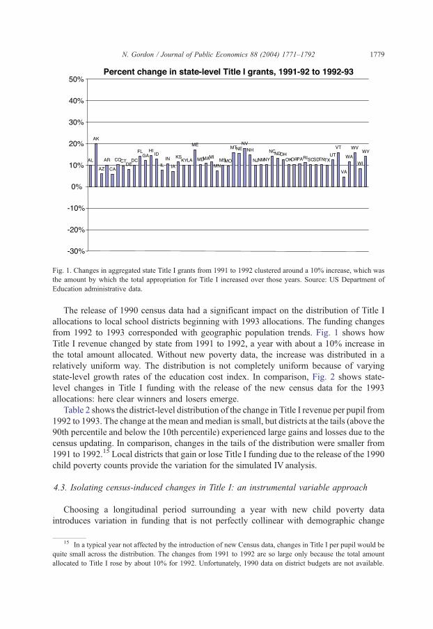
Fig. 1. Changes in aggregated state Title I grants from 1991 to 1992 clustered around a 10% increase, which was
the amount by which the total appropriation for Title I increased over those years. Source: US Department of
Education administrative data.
N. Gordon / Journal of Public Economics 88 (2004) 1771–1792 1779
The release of 1990 census data had a significant impact on the distribution of Title I
allocations to local school districts beginning with 1993 allocations. The funding changes
from 1992 to 1993 corresponded with geographic population trends. Fig. 1 shows how
Title I revenue changed by state from 1991 to 1992, a year with about a 10% increase in
the total amount allocated. Without new poverty data, the increase was distributed in a
relatively uniform way. The distribution is not completely uniform because of varying
state-level growth rates of the education cost index. In comparison, Fig. 2 shows state-
level changes in Title I funding with the release of the new census data for the 1993
allocations: here clear winners and losers emerge.
Table 2 shows the district-level distribution of the change in Title I revenue per pupil from
1992 to 1993. The change at the mean andmedian is small, but districts at the tails (above the
90th percentile and below the 10th percentile) experienced large gains and losses due to the
census updating. In comparison, changes in the tails of the distribution were smaller from
1991 to 1992.15 Local districts that gain or lose Title I funding due to the release of the 1990
child poverty counts provide the variation for the simulated IV analysis.
4.3. Isolating census-induced changes in Title I: an instrumental variable approach
Choosing a longitudinal period surrounding a year with new child poverty data
introduces variation in funding that is not perfectly collinear with demographic change
15 In a typical year not affected by the introduction of new Census data, changes in Title I per pupil would be
quite small across the distribution. The changes from 1991 to 1992 are so large only because the total amoun
allocated to Title I rose by about 10% for 1992. Unfortunately, 1990 data on district budgets are not available
t
.
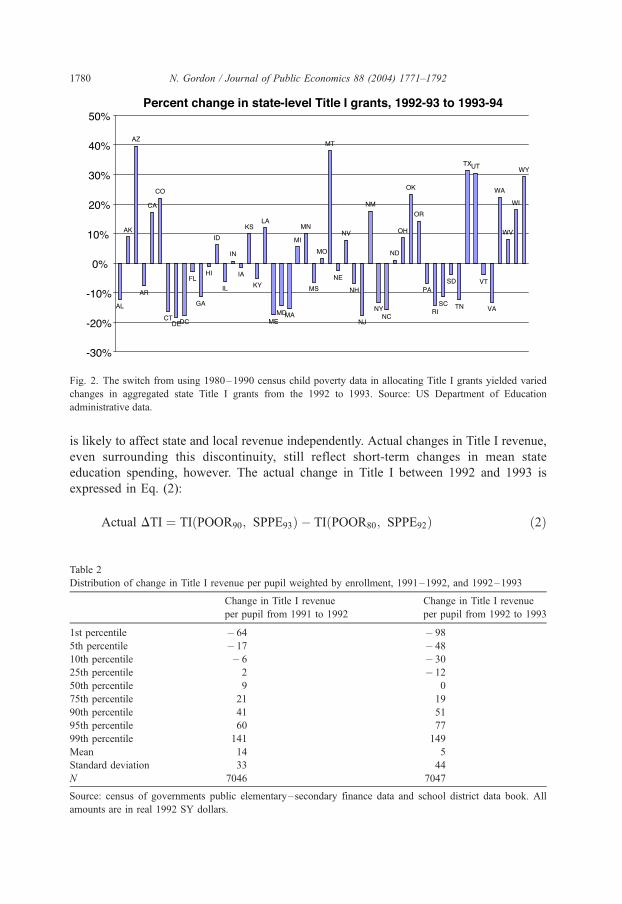
Fig. 2. The switch from using 1980–1990 census child poverty data in allocating Title I grants yielded varied
changes in aggregated state Title I grants from the 1992 to 1993. Source: US Department of Education
administrative data.
N. Gordon / Journal of Public Economics 88 (2004) 1771–17921780
is likely to affect state and local revenue independently. Actual changes in Title I revenue,
even surrounding this discontinuity, still reflect short-term changes in mean state
education spending, however. The actual change in Title I between 1992 and 1993 is
expressed in Eq. (2):
Actual DTI ¼ TIðPOOR90; SPPE93Þ � TIðPOOR80; SPPE92Þ ð2Þ
Table 2
Distribution of change in Title I revenue per pupil weighted by enrollment, 1991–1992, and 1992–1993
Change in Title I revenue
per pupil from 1991 to 1992
Change in Title I revenue
per pupil from 1992 to 1993
1st percentile � 64 � 98
5th percentile � 17 � 48
10th percentile � 6 � 30
25th percentile 2 � 12
50th percentile 9 0
75th percentile 21 19
90th percentile 41 51
95th percentile 60 77
99th percentile 141 149
Mean 14 5
Standard deviation 33 44
N 7046 7047
Source: census of governments public elementary–secondary finance data and school district data book. All
amounts are in real 1992 SY dollars.
N. Gordon / Journal of Public Economics 88 (2004) 1771–1792 1781
Because I wish to consider the effect of an exogenous shift in Title I funds (based solely
on introduction of 1990 census data), I calculate how Title I revenue would change with
the new poverty data, holding mean per-pupil spending in each state constant. This
‘‘census-determined’’ change in Title I is given by the following equation:
Census-determined DTI ¼ TIðPOOR90; SPPE93Þ � TIðPOOR80; SPPE93Þ ð3Þ
We do not observe this change, but I can calculate it using the Title I formula, poverty
data, and state per-pupil spending. I use the calculated census-determined change as an
instrument for the actual change in Title I revenue.
To compute the census-determined change, I first calculate how much Title I revenue
per pupil school districts would have received in 1993 if the poverty counts had not been
updated but all other inputs to the allocation had changed. In this calculation, the total
amount of Title I grants distributed is equal to the 1993 amount, and SPPE is equal to the
level used for that state in the 1993 allocations; the allocation is denoted by TI(POOR80,
SPPE93). I then calculate the difference between the actual 1993 per-pupil Title I revenue
amount and this calculated per-pupil amount for each district.
Because any given change in total funding is differentially important to districts with
more or fewer students, I analyze changes in Title I funding per student. Thus, my
simulated variable is the census-determined change in Title I per pupil:16
TI93ðPOOR90; SPPE93ÞENROLLMENT93
� TISIMðPOOR80; SPPE93ÞENROLLMENT92
It is an instrument for the actual change in Title I per pupil:
TI93ðPOOR90; SPPE93ÞENROLLMENT93
� TI92ðPOOR80; SPPE92ÞENROLLMENT92
I also consider 3-year changes in Title I revenue per pupil. In this case the simulated
variable is:
TI95ðPOOR90; SPPE95ÞENROLLMENT95
� TISIMðPOOR80; SPPE95ÞENROLLMENT92
4.4. Impact of Title I on school district budgets: estimation
I assess the impact of the simulated exogenous change in Title I revenue per pupil on a
variety of school district budgetary variables. I examine impacts on total revenue, local
revenue, state revenue and its components, and federal revenue. I also consider effects on
instructional spending, spending on support services (the next largest category of
16 The instrument divides simulated Title I by enrollment in 1992 rather than 1993 in case districts
experience large changes in enrollment between 1992 and 1993 that would drive the difference between the
instrument and the actual Title I change per pupil. Results are nearly identical, however, using the 1993
enrollment in the denominator.
N. Gordon / Journal of Public Economics 88 (2004) 1771–17921782
educational spending), and capital outlay expenditures. I use all measures at the per-pupil
level throughout the analysis.
Because I use first-differences at the district-level, I am controlling for all fixed district-
level characteristics. The differencing does not, however, control for concurrent district-
specific changes unrelated to the causal impact of Title I during the relevant period. I,
therefore, control for pre-existing district-level trends in state and local revenue per pupil
with changes in state and local revenue per pupil from 1986 to 1991 (spending is highly
correlated with the sum of state and local revenue).
Eq. (4) shows the regression specification for the effect of changes in Title I per pupil
(DTI PP) on changes in instructional expenditure per pupil (DINST EXP PP), controlling
for lagged changes in district-level state and local revenue per pupil (from 1986 to 1991,
lag DSTATE REV PP and lag DLOCAL REV PP), and enrollment changes:
DINST EXP PPd ¼ ad þ b*DTI PPd þ /*lag DSTATE REV PPd
þ c*lag DLOCAL REV PPd þ h* DENROLLMENTd þ ed ð4Þ
where the census-determined change in Title I per pupil instruments for the actual change
in Title I per pupil and d indexes the school district. The specification remains the same for
other dependent variables. I use the same lagged changes in district-level state and local
revenue per pupil for both the 1- and 3-year specifications, as well as in the first stage.
4.5. First stage results
Table 3 shows that the simulated change in Title I grants is a strong predictor of the
actual change. These are effectively the first stage regressions of the IV procedure for the
1- and 3-year changes. The simulated census-determined change in Title I grants per
pupil from 1992 to 1993 (at the district level) predict the actual change in Title I grants
per pupil over that period quite well: in a simple regression predicting the actual change,
the coefficient on the simulated change is 0.58 and the standard error (S.E.) is 0.04, with
Table 3
First-stage results: correlations between simulated and actual changes in Title I revenue per pupil
Dependent variable Independent variable Coefficient (S.E.) F R2
Actual change in Title I
per pupil, 1992–1993
Simulated change in Title I
per pupil, 1992–1993
0.584 (0.040) 91 0.526
Actual change in Title I
per pupil, 1992–1995
Simulated change in Title I
per pupil, 1992–1995
0.672 (0.022) 291 0.630
Simulated change in Title I per pupil are calculated holding child poverty at 1980 levels. Regression results are
weighted by 1992 enrollment of district. Robust S.E. are in parentheses. All amounts are in real 1992 SY dollars.
One-year changes include Michigan; 3-year changes do not. One-year results excluding Michigan are quite close
to those reported here including Michigan. All results exclude the following states: AK, DC, HI, MT, NE, NH,
TX, and VT. Regressions control for district-level trends in state and local per-pupil revenue from 1986 to 1991
and for enrollment changes from 1992 to 1993, but are not sensitive to the exclusion of these controls.
N. Gordon / Journal of Public Economics 88 (2004) 1771–1792 1783
an R2 of 0.526 and an F-statistic of 91. The simulated census-determined per-pupil
change over the 3-year period is a strong predictor of that actual change as well: the
coefficient on the simulated change is 0.67 and the S.E. is 0.02, with an R2 of 0.630 and
an F-statistic of 291.
That the coefficients on the simulated per-pupil changes are consistently less than one is
not inconsistent with the strong predictive power of the instrument. To isolate the effect of
the poverty data updating, the census-determined per-pupil changes are simulated using
different levels of mean SPPE than were used in the actual allocation process. There are
also several potential sources of measurement error. There is likely reporting error in the
Census of Governments, particularly about which parts of Title I are reported.17 The
census poverty data from 1980 and 1990, coded at the school district-level, also contain
reporting error. The hold-harmless clause may introduce some simulation error. These
factors contribute to classical measurement error, which is exacerbated by taking first
differences, as this approach requires. Regressing my computed levels of Title I per pupil
for 1992 on actual corresponding levels of Title I per pupil gives a coefficient of 0.97,
while regressing my computed census-determined changes in Title I per pupil from 1992
to 1993 on actual corresponding changes gives a coefficient of 0.58.
5. Data
My empirical strategy of identifying exogenous changes in Title I funding and
analyzing how these changes affect expenditures and revenues requires school district-
level data on the number of children and poor children in each district as measured in the
1980 and 1990 censuses and school district-level enrollments, Title I grant amounts,
expenditures, and revenues for 1991 through 1995.
Annual financial data at the school district level for 1991 through 1995 come from the
Elementary–Secondary School District Financial Data collected by the Bureau of the
Census. This data set gives the total Title I allocation for each district in each year without
distinguishing between basic and concentration grants. It also provides revenues and
expenditures, by category, for each school district. I use measures of Title I revenue,
spending on instruction and on support services, capital outlays, enrollment, local revenue,
state formula aid, and state categorical aid from these data.
In the simulation process, I use Department of Education administrative data at the
county level for 1991 through 1995 on the number of formula count children eligible
for basic and concentration grants, adjusted spending per pupil by state, and actual
basic and concentration grant Title I allocations. Decennial data on the total number of
children and children in poverty at the school district-level come from the Summary
Tape File 3F for the 1980 US Census of Populations and from the joint Census-
National Center for Education Statistics School District Data Book for the 1990 US
Census of Populations.
17 Examination of administrative data suggests that some districts report revenue for migrant education or
Even Start, technically Title I programs, while other districts with migrant education or Even Start funds only
report revenue for Title I, Part A.
Table 4
Summary revenue and expenditure statistics for 1992, by whether school districts are predicted to gain or lose
Title I funds with census updating, weighted by district enrollment
Gainers Losers All
Fall enrollment 87,641 (231,159) 36,338 (75,345) 63,985 (179,061)
Title I revenue per pupil 138 (108) 148 (132) 143 (120)
Total expenditure per pupil 5742 (1662) 6089 (1940) 5902 (1804)
Elementary and secondary
expenditure per pupil
4980 (1362) 5373 (1665) 5161 (1522)
Instructional expenditure per pupil 3073 (937) 3329 (1081) 3191 (1014)
Support services expenditure per pupil 1667 (506) 1804 (646) 1730 (579)
Expenditures for capital outlay per pupil 498 (577) 449 (599) 475 (588)
Expenditures for other educational
services per pupil
264 (231) 267 (301) 266 (265)
State revenue per pupil 2710 (875) 2668 (1139) 2691 (1006)
State formula aid per pupil 1937 (814) 1778 (977) 1864 (897)
State categorical aid per pupil 773 (478) 890 (530) 827 (506)
Local revenue per pupil 2531 (1584) 3038 (1964) 2765 (1787)
Number of observations 3475 3572 7047
Means are reported, with standard deviations in parentheses. All figures are in real SY 1992 dollars. Results are
weighted by 1992 enrollment.
N. Gordon / Journal of Public Economics 88 (2004) 1771–17921784
Per-pupil amounts of Title I changes are more accurately replicated (and thus
simulated) for larger school districts. I use a combination cutoff and weighting method
to minimize the impact of small school district replication error, limiting the sample to
school districts with enrollments of at least 200 students in each year of the analysis and
weighting school districts by their 1992 enrollments.18 This strategy avoids using the most
error-laden school districts with fewer than 200 students, and relies more heavily on the
larger districts with the cleanest replication. These districts are also of greater policy
interest, as they receive the bulk of Title I funding. The majority of dropped districts were
dropped because they were missing in the data from at least one of the key years and thus
did not merge into my final sample. I also dropped all districts from certain states
problematic in this context.19
Table 4 presents summary statistics for my key variables, dividing the sample into
school districts predicted to gain Title I funds with the census updating and those
predicted to lose funds. This divides the sample into roughly equal groups, with 3475
districts predicted to gain funds and 3572 predicted to lose funds. Districts predicted to
18 Because Title I funds are given to districts per formula count student, while administering a Title I program
incurs some level of fixed administrative costs, small districts have lower take-up rates on Title I participation
given eligibility.19 I dropped Alaska, the District of Columbia, and Hawaii because of their unique geographic and political
characteristics. I dropped Montana, Nebraska, New Hampshire, and Vermont because these states have
undistributed concentration grants, making it difficult to simulate Title I allocations. Finally, I exclude Texas for
all years, and exclude Michigan for the 3-year changes, due to dramatic state school finance reforms which make
it impossible to determine which changes in state and local revenue result from changes in Title I rather than
changes in school finance regimes. Results for 1-year changes are not sensitive to the inclusion of Michigan.
N. Gordon / Journal of Public Economics 88 (2004) 1771–1792 1785
gain funds are on average larger than those losing funds, but other differences between
districts are small.
6. Results
I examine short-run responses to Title I changes over the first year following the use of
the 1990 census in the allocations, from the 1992 to 1993 school years, over the 2-year
period from 1992 to 1994, and longer-run responses for the 3-year change from 1992 to
1995. My discussion focuses on the IV results in columns 1 and 3 in Table 5, which
present results for 1- and 3-year changes. The 2-year changes, in column 2, generally fall
about midway between the 1- and 3-year changes. OLS results, which are largely
consistent with the IV results in Table 5, are reported in the Appendix A.20 All regression
results are in per-pupil terms.
6.1. Short-run responses to census-determined changes in Title I
In the first year following census updating, Title I exhibits classic flypaper properties. It
sticks about dollar for dollar to total revenue and to instructional spending, without inducing
offsetting responses in local or state education revenue. Column 1 of Table 5 reports IV
estimates of the effects of census-determined changes in Title I per pupil for the 1-year period
following the introduction of the new census data. The first line shows the effect on total
revenue, which is the sum of effects on state, local, and federal revenue.21 A $1 increase in
Title I translates into a $0.98 increase in total revenue (with a S.E. of 0.41) and a $1.40
increase in instructional spending (with a S.E. of 0.55), with both effects significant at the
5% level. S.E. in all of the analyses are sufficiently large, however, that I emphasize the
direction and significance of results throughout and caution against strict interpretation of
specific coefficients. More generally, then, changes in total revenue and instructional
spending for the 1-year period are significantly positive and insignificantly different from
one.
Table 5 first breaks down the response in total revenue into state, local, and federal
components. I also group state revenue to school districts into two categories: formula aid,
which typically is determined by formulas dependent on property values and local revenue
effort, and categorical aid. Categorical aid is distributed for specific programs, including
programs such as compensatory education and special education that disproportionately go
to poor districts, and is based on characteristics of students in the school district.22
20 The main difference between the OLS and IV results arises in predicting changes in state aid to districts.
This is unsurprising, as the use of instrument is motivated by potential correlations between actual changes in
Title I and trends in state aid to districts.21 Note that the federal revenue effects are insignificantly different from one for all 3 years because they are
dominated by actual changes in Title I, but are not exactly one because school districts receive other federal
revenue and because this category includes actual Title I revenue rather than simulated.22 About two-thirds of state education revenue nationwide is distributed through formula aid, and about one-
third through categorical aid. These proportions, and the types of categorical aid provided, vary by state.
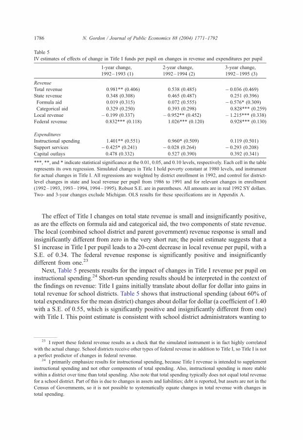
Table 5
IV estimates of effects of change in Title I funds per pupil on changes in revenue and expenditures per pupil
1-year change,
1992–1993 (1)
2-year change,
1992–1994 (2)
3-year change,
1992–1995 (3)
Revenue
Total revenue 0.981** (0.406) 0.538 (0.485) � 0.036 (0.469)
State revenue 0.348 (0.308) 0.465 (0.487) 0.251 (0.396)
Formula aid 0.019 (0.315) 0.072 (0.555) � 0.576* (0.309)
Categorical aid 0.329 (0.250) 0.393 (0.298) 0.828*** (0.259)
Local revenue � 0.199 (0.337) � 0.952** (0.452) � 1.215*** (0.338)
Federal revenue 0.832*** (0.118) 1.026*** (0.120) 0.928*** (0.130)
Expenditures
Instructional spending 1.401** (0.551) 0.960* (0.509) 0.119 (0.501)
Support services � 0.425* (0.241) � 0.028 (0.264) � 0.293 (0.208)
Capital outlays 0.478 (0.332) 0.527 (0.390) 0.392 (0.341)
***, **, and * indicate statistical significance at the 0.01, 0.05, and 0.10 levels, respectively. Each cell in the table
represents its own regression. Simulated changes in Title I hold poverty constant at 1980 levels, and instrument
for actual changes in Title I. All regressions are weighted by district enrollment in 1992, and control for district-
level changes in state and local revenue per pupil from 1986 to 1991 and for relevant changes in enrollment
(1992–1993, 1993–1994, 1994–1995). Robust S.E. are in parentheses. All amounts are in real 1992 SY dollars.
Two- and 3-year changes exclude Michigan. OLS results for these specifications are in Appendix A.
N. Gordon / Journal of Public Economics 88 (2004) 1771–17921786
The effect of Title I changes on total state revenue is small and insignificantly positive,
as are the effects on formula aid and categorical aid, the two components of state revenue.
The local (combined school district and parent government) revenue response is small and
insignificantly different from zero in the very short run; the point estimate suggests that a
$1 increase in Title I per pupil leads to a 20-cent decrease in local revenue per pupil, with a
S.E. of 0.34. The federal revenue response is significantly positive and insignificantly
different from one.23
Next, Table 5 presents results for the impact of changes in Title I revenue per pupil on
instructional spending.24 Short-run spending results should be interpreted in the context of
the findings on revenue: Title I gains initially translate about dollar for dollar into gains in
total revenue for school districts. Table 5 shows that instructional spending (about 60% of
total expenditures for the mean district) changes about dollar for dollar (a coefficient of 1.40
with a S.E. of 0.55, which is significantly positive and insignificantly different from one)
with Title I. This point estimate is consistent with school district administrators wanting to
23 I report these federal revenue results as a check that the simulated instrument is in fact highly correlated
with the actual change. School districts receive other types of federal revenue in addition to Title I, so Title I is not
a perfect predictor of changes in federal revenue.24 I primarily emphasize results for instructional spending, because Title I revenue is intended to supplement
instructional spending and not other components of total spending. Also, instructional spending is more stable
within a district over time than total spending. Also note that total spending typically does not equal total revenue
for a school district. Part of this is due to changes in assets and liabilities; debt is reported, but assets are not in the
Census of Governments, so it is not possible to systematically equate changes in total revenue with changes in
total spending.
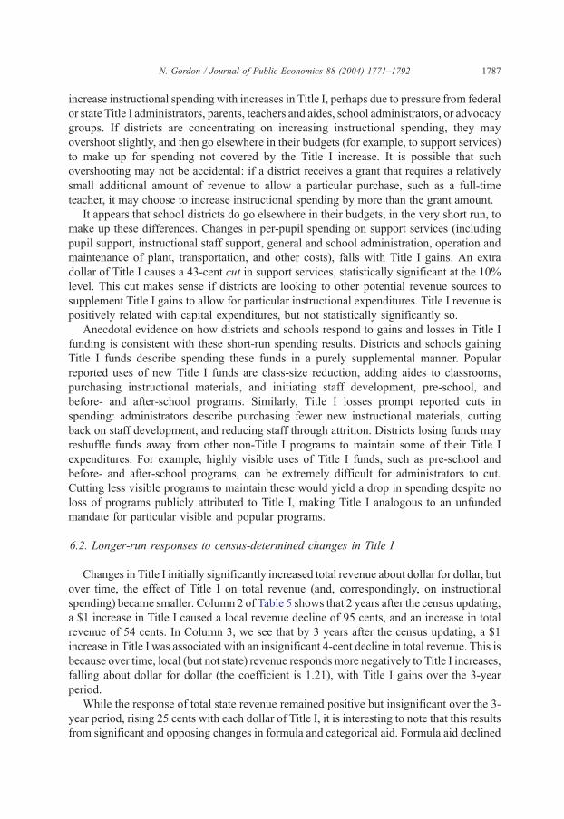
N. Gordon / Journal of Public Economics 88 (2004) 1771–1792 1787
increase instructional spending with increases in Title I, perhaps due to pressure from federal
or state Title I administrators, parents, teachers and aides, school administrators, or advocacy
groups. If districts are concentrating on increasing instructional spending, they may
overshoot slightly, and then go elsewhere in their budgets (for example, to support services)
to make up for spending not covered by the Title I increase. It is possible that such
overshooting may not be accidental: if a district receives a grant that requires a relatively
small additional amount of revenue to allow a particular purchase, such as a full-time
teacher, it may choose to increase instructional spending by more than the grant amount.
It appears that school districts do go elsewhere in their budgets, in the very short run, to
make up these differences. Changes in per-pupil spending on support services (including
pupil support, instructional staff support, general and school administration, operation and
maintenance of plant, transportation, and other costs), falls with Title I gains. An extra
dollar of Title I causes a 43-cent cut in support services, statistically significant at the 10%
level. This cut makes sense if districts are looking to other potential revenue sources to
supplement Title I gains to allow for particular instructional expenditures. Title I revenue is
positively related with capital expenditures, but not statistically significantly so.
Anecdotal evidence on how districts and schools respond to gains and losses in Title I
funding is consistent with these short-run spending results. Districts and schools gaining
Title I funds describe spending these funds in a purely supplemental manner. Popular
reported uses of new Title I funds are class-size reduction, adding aides to classrooms,
purchasing instructional materials, and initiating staff development, pre-school, and
before- and after-school programs. Similarly, Title I losses prompt reported cuts in
spending: administrators describe purchasing fewer new instructional materials, cutting
back on staff development, and reducing staff through attrition. Districts losing funds may
reshuffle funds away from other non-Title I programs to maintain some of their Title I
expenditures. For example, highly visible uses of Title I funds, such as pre-school and
before- and after-school programs, can be extremely difficult for administrators to cut.
Cutting less visible programs to maintain these would yield a drop in spending despite no
loss of programs publicly attributed to Title I, making Title I analogous to an unfunded
mandate for particular visible and popular programs.
6.2. Longer-run responses to census-determined changes in Title I
Changes in Title I initially significantly increased total revenue about dollar for dollar, but
over time, the effect of Title I on total revenue (and, correspondingly, on instructional
spending) became smaller: Column 2 of Table 5 shows that 2 years after the census updating,
a $1 increase in Title I caused a local revenue decline of 95 cents, and an increase in total
revenue of 54 cents. In Column 3, we see that by 3 years after the census updating, a $1
increase in Title I was associated with an insignificant 4-cent decline in total revenue. This is
because over time, local (but not state) revenue responds more negatively to Title I increases,
falling about dollar for dollar (the coefficient is 1.21), with Title I gains over the 3-year
period.
While the response of total state revenue remained positive but insignificant over the 3-
year period, rising 25 cents with each dollar of Title I, it is interesting to note that this results
from significant and opposing changes in formula and categorical aid. Formula aid declined
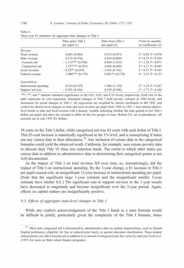
Table 6
Three-year IV estimates, by aggregate state changes in Title I
State gains Title I
per pupil (1)
State loses Title I
per pupil (2)
F-test on equality
of coefficients (3)
Revenue
Total revenue 0.683 (0.484) 0.515 (0.973) F = 0.02 P= 0.878
State revenue 0.123 (0.476) 0.924 (0.809) F = 0.73 P= 0.394
Formula aid � 1.113*** (0.396) 0.880 (1.032) F = 3.25 P= 0.071
Categorical aid 1.237*** (0.391) 0.044 (0.440) F = 4.11 P= 0.043
Local revenue � 0.527* (0.294) � 1.010 (0.741) F = 0.37 P= 0.545
Federal revenue 1.086*** (0.170) 0.601** (0.278) F = 2.21 P= 0.137
Expenditures
Instructional spending 0.214 (0.195) 1.486 (1.129) F = 1.23 P= 0.267
Support services � 0.283 (0.186) 0.539 (0.590) F = 1.77 P= 0.184
***, **, and * indicate statistical significance at the 0.01, 0.05, and 0.10 levels, respectively. Each row in the
table represents its own regression. Simulated changes in Title I hold poverty constant at 1980 levels, and
instrument for actual changes in Title I. All regressions are weighted by district enrollment in fall 1992, and
control for district-level changes in state and local revenue per pupil from 1986 to 1991. I also interact district-
level trends in state and local revenue with a dummy variable indicating whether the state gained or lost Title I
dollars per pupil, and allow the constant to differ for the two groups of states. Robust S.E. are in parentheses. All
amounts are in real 1992 SY dollars.
N. Gordon / Journal of Public Economics 88 (2004) 1771–17921788
58 cents on the Title I dollar, while categorical aid rose 83 cents with each dollar of Title I.
This 83-cent increase is statistically significant at the 1% level, and is unsurprising if states
use any census data in their allocations.25 Any inclusion of census data in the categorical
formulas could yield the observed result. California, for example, uses census poverty data
to allocate their Title VI class size reduction funds. The extent to which other states use
census data in addition to administrative data in determining their categorical grants is not
well documented.
As the impact of Title I on total revenue fell over time, so, unsurprisingly, did the
impact of Title I on instructional spending. By the 3-year change, a $1 increase in Title I
per pupil caused only an insignificant 12-cent increase in instructional spending per pupil.
(Note that the significant large 1-year estimate and the insignificant smaller 3-year
estimate have similar S.E.) The significant cuts in support services in the 1-year results
have decreased in magnitude and become insignificant over the 3-year period. Again,
effects on capital outlays are insignificantly positive.
6.3. Effects of aggregate state-level changes in Title I
While any explicit acknowledgement of the Title I funds in a state formula would
be difficult to justify, particularly given the complexity of the Title I formula, states
25 Most state categorical aid is determined by administrative data on student characteristics, such as limited
English proficiency, eligibility for free or reduced price lunch, or special education classification. These student
characteristics can affect formula aid in addition to or instead of categorical aid; this varies by state (see Gold et al.
(1995) for more on State school finance programs).
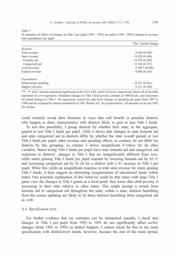
Table 7
IV estimates of effects of changes in Title I per pupil (1992–1993) on earlier (1991–1992) changes in revenue
and expenditures per pupil
‘‘Pre’’ period change
Revenue
Total revenue 0.340 (0.369)
State revenue � 0.528 (0.340)
Formula aid � 0.339 (0.289)
Categorical aid � 0.188 (0.272)
Local revenue 0.780* (0.448)
Federal revenue 0.088 (0.103)
Expenditures
Instructional spending � 0.327 (0.261)
Support services 0.121 (0.184)
***, **, and * indicate statistical significance at the 0.01, 0.05, and 0.10 levels, respectively. Each cell in the table
represents its own regression. Simulated changes in Title I hold poverty constant at 1980 levels, and instrument
for actual changes in Title I. All regressions control for state-level changes in spending per pupil from 1987 to
1990 and are weighted by district enrollment in 1992. Robust S.E. are in parentheses. All amounts are in real 1992
SY dollars.
N. Gordon / Journal of Public Economics 88 (2004) 1771–1792 1789
could certainly tweak their formulas in ways that will benefit or penalize districts
who happen to share characteristics with districts likely to gain or lose Title I funds.
To test this possibility, I group districts by whether their state, in the aggregate,
gained or lost Title I funds per pupil. Table 6 shows that changes in state formula aid
and state categorical aid to districts differ by whether the state overall gained or lost
Title I funds per pupil; other revenue and spending effects, in contrast, do not differ for
districts by this grouping, as column 3 shows insignificant F-values for all other
variables. States losing Title I funds per pupil have state formula aid and categorical aid
responses to districts’ changes in Title I that are insignificantly different from zero,
while states gaining Title I funds per pupil respond by lowering formula aid by $1.11
and increasing categorical aid by $1.24 for a district with a $1 increase in Title I per
pupil. While this yields an insignificant response in total state revenue for states gaining
Title I funds, it does suggest an interesting reorganization of educational funds within
states. One potential explanation of this behavior could be that states with large Title I
gains view the changes in Title I grants as a focal point: they know that child poverty is
increasing in their state relative to other states. This might prompt a switch from
formula aid to categorical aid throughout the state; within a state, districts benefiting
from the census updating are likely to be those districts benefiting from categorical aid
as well.
6.4. Specification tests
For further evidence that my estimates can be interpreted causally, I check that
changes in Title I per pupil from 1992 to 1993 do not significantly affect earlier
changes (from 1991 to 1992) in district budgets. I cannot check for this in my main
specification with district-level trends, however, because the end of the trend period,

N. Gordon / Journal of Public Economics 88 (2004) 1771–17921790
the 1991 school year, I control for pre-existing state-level trends in spending per pupil
from 1986 to 1990.26
Table 7 shows that the change in Title I per pupil from 1992 to 1993 does not have
predictive power for earlier changes in state, federal, or total revenue, or for spending on
instruction or support services, in the ‘‘pre-period’’ test controlling for state trends in
spending per pupil. For example, a dollar increase in Title I per pupil from 1992 to 1993
(using the simulated change as an instrument for the actual change) is associated with a 34-
cent increase in total revenue per pupil from 1991 to 1992, with a S.E. of 0.37, controlling
for state trends.
While the 1992–1993 Title I change does have predictive power in the preceding
period for local revenue, the direction of this effect suggests that any pre-existing trend is
swamped by Title I, rather than the Title I effect being driven by a pre-existing trend. A
district receiving a $1 increase in Title I would have experienced a 78-cent increase in
local revenue in the previous year (with a S.E. of 0.45); when controlling for district-level
trends in the later period (rather than state-level trends in the ‘‘pre’’ period), however, local
revenue falls.
7. Conclusions
This paper finds that while school districts comply with the letter of the law, Title I
ultimately fails to fully meet the spirit of its mandate to supplement instructional
spending. Title I increases initially boost total school district revenue and instructional
spending about dollar for dollar, but by the third year following the census-determined
Title I changes, the effects are no longer significantly positive in the full sample, due to
local government reactions countering the effects of Title I. These local reactions occur
across all regions and regardless of aggregate state-level changes, but state revenue
reactions to individual districts differ by state-level changes in Title I. States with
increases in Title I are more likely to move from formula to categorical aid. Because
the local reactions rendering Title I changes insignificant to instructional spending
generally do not violate the maintenance of effort mandate of the legislation, the federal
government cannot counter these responses simply by increasing enforcement of existing
compliance mechanisms.
These results further the literature on the flypaper effect along several dimensions.
First, by following the effects of Title I changes on school district budgets for 3 years,
I can examine the dynamics of the flypaper effect. A 1-year analysis of these data
would suggest that the grant is quite sticky, while the 3-year analysis shows otherwise.
This suggests that research on other flypaper effects would benefit from looking at
changes in responses over time, rather than longitudinal changes immediately
26 While district-level trends would be a preferable control to state-level trends, district-level spending per
pupil is available only every 5 years before the beginning of the ‘‘pre’’ period. The end of the trend period, the
1991 school year, is the start of the ‘‘pre’’ period, causing a mechanical correlation between the trend period and
the ‘‘pre’’ period.

N. Gordon / Journal of Public Economics 88 (2004) 1771–1792 1791
surrounding a policy change. Second, the finance structure of education allows me to
consider the response of the receiving jurisdiction (the school district) as well as an
intermediate jurisdiction (the state) to the grant from the issuing jurisdiction (the
federal government). I observe that local districts are more active in their revenue
responses to intergovernmental grants than are the intermediate state agencies. Finally,
my identification strategy relies on changes in reported data rather than changes in
actual conditions, thus providing a particularly strong foundation for drawing inference.
Other work may find flypaper effects that are statistical artifacts, if it does not use
adequately exogenous variation in the grants received or does not follow effects over
time.
Education research should be informed by this work as well. Researchers asking if
money matters must first establish that the money is spent in ways that should matter,
rather than evaluating partial equilibrium effects of any particular revenue stream. This
research furthers the evaluation literature on Title I specifically by revealing how
revenue and spending react to changes in Title I at state and local levels. Because the
identification relies on the discrete change in funding surrounding the release of new
census data, it limits our interpretation of the estimate. Title I has existed since 1965,
and while the average district experienced full crowd-out of the changes studied, it is
possible that earlier changes were in fact supplemental.
Important questions about Title I’s effects on social welfare remain. First, what form
do the crowd-out responses to Title I take, and how do they affect welfare? Does the
incidence in benefits or costs from Title I-induced changes in local property tax rates or
state and/or local spending patterns favor the disadvantaged population targeted by the
program? Second, how are any supplemental Title I funds distributed within school
districts and schools? Even in districts where large shares of Title I revenue continue to
stick to instructional spending at the district-level over time, benefits may not be
appropriately targeted to poor schools within school districts, or to educationally-
disadvantaged students within schools. Answers to these questions can provide impor-
tant guidance in assessing the efficacy of the federal government’s targeting of education
funds to the poor.
Acknowledgements
I am especially grateful to Caroline Hoxby. I thank Katherine Baicker, David Cutler,
Amy Finkelstein, Claudia Goldin, Jonathan Gruber, Brian Jacob, Mireille Jacobson,
Christopher Jencks, Lawrence Katz, Sarah Reber, Janice Seinfeld, Tara Watson, and two
referees for their suggestions, as well as seminar participants at Harvard, UCSD, RAND,
UC Santa Cruz, the Harris School, the New York Fed, Georgetown Public Policy Institute,
Berkeley, UT Dallas, UCLA, UC Davis, and the NBER Government Expenditure
Universities’ Research Conference. Paul Brown of the US Department of Education
generously provided administrative data and detailed explanation of the Title I formula.
Any remaining errors are my own. I am grateful for support from the Spencer Foundation
and the American Educational Research Association, neither of which are responsible for
the contents of this paper.
N. Gordon / Journal of Public Economics 88 (2004) 1771–17921792
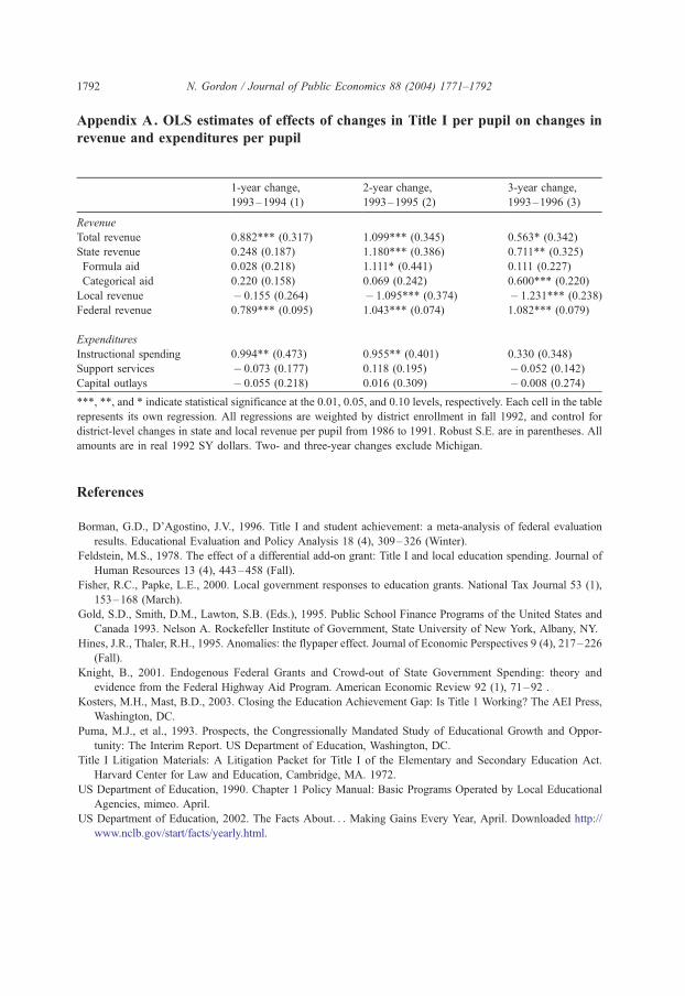
Appendix A. OLS estimates of effects of changes in Title I per pupil on changes in
revenue and expenditures per pupil
1-year change,
1993–1994 (1)
2-year change,
1993–1995 (2)
3-year change,
1993–1996 (3)
Revenue
Total revenue 0.882*** (0.317) 1.099*** (0.345) 0.563* (0.342)
State revenue 0.248 (0.187) 1.180*** (0.386) 0.711** (0.325)
Formula aid 0.028 (0.218) 1.111* (0.441) 0.111 (0.227)
Categorical aid 0.220 (0.158) 0.069 (0.242) 0.600*** (0.220)
Local revenue � 0.155 (0.264) � 1.095*** (0.374) � 1.231*** (0.238)
Federal revenue 0.789*** (0.095) 1.043*** (0.074) 1.082*** (0.079)
Expenditures
Instructional spending 0.994** (0.473) 0.955** (0.401) 0.330 (0.348)
Support services � 0.073 (0.177) 0.118 (0.195) � 0.052 (0.142)
Capital outlays � 0.055 (0.218) 0.016 (0.309) � 0.008 (0.274)
***, **, and * indicate statistical significance at the 0.01, 0.05, and 0.10 levels, respectively. Each cell in the table
represents its own regression. All regressions are weighted by district enrollment in fall 1992, and control for
district-level changes in state and local revenue per pupil from 1986 to 1991. Robust S.E. are in parentheses. All
References
Borman, G.D., D’Agostino, J.V., 1996. Title I and student achievement: a meta-analysis of federal evaluation
results. Educational Evaluation and Policy Analysis 18 (4), 309–326 (Winter).
Feldstein, M.S., 1978. The effect of a differential add-on grant: Title I and local education spending. Journal of
Human Resources 13 (4), 443–458 (Fall).
Fisher, R.C., Papke, L.E., 2000. Local government responses to education grants. National Tax Journal 53 (1),
153–168 (March).
Gold, S.D., Smith, D.M., Lawton, S.B. (Eds.), 1995. Public School Finance Programs of the United States and
Canada 1993. Nelson A. Rockefeller Institute of Government, State University of New York, Albany, NY.
Hines, J.R., Thaler, R.H., 1995. Anomalies: the flypaper effect. Journal of Economic Perspectives 9 (4), 217–226
(Fall).
Knight, B., 2001. Endogenous Federal Grants and Crowd-out of State Government Spending: theory and
evidence from the Federal Highway Aid Program. American Economic Review 92 (1), 71–92 .
Kosters, M.H., Mast, B.D., 2003. Closing the Education Achievement Gap: Is Title 1 Working? The AEI Press,
Washington, DC.
Puma, M.J., et al., 1993. Prospects, the Congressionally Mandated Study of Educational Growth and Oppor-
tunity: The Interim Report. US Department of Education, Washington, DC.
Title I Litigation Materials: A Litigation Packet for Title I of the Elementary and Secondary Education Act.
Harvard Center for Law and Education, Cambridge, MA. 1972.
US Department of Education, 1990. Chapter 1 Policy Manual: Basic Programs Operated by Local Educational
Agencies, mimeo. April.
US Department of Education, 2002. The Facts About. . . Making Gains Every Year, April. Downloaded http://
www.nclb.gov/start/facts/yearly.html.
amounts are in real 1992 SY dollars. Two- and three-year changes exclude Michigan.