distribution and growth - hans-böckler-stiftung - … · on equilibrium growth rate ......

1

Distribution and Growth

Eckhard Hein

6h International Summer School on

‘Keynesian Macroeconomics and European Economic Policies’

FMM

30 July – 5 August 2017, Berlin, Germany

2

Structure • The post-Keynesian (and the classical and Marxian)

vs. the neoclassical approaches towards distribution and growth

• The post-Kaleckian distribution and growth model: theory and empirical results

• Interest, credit, financialisation and distribution and growth

• Debates around the Kaleckian distribution and growth models

4

Here and today: Selections from Chapters 7, 9, 10

2014

5






6

Table 1: Distribution and growth theories

Orthodox Heterodox

Old

neoclassical

(Solow,

Swan)

New

neoclassical

(Romer,

Lucas)

Classical/

Marxian

Post-Keynesian

Kaldor-

Robinson

Kalecki-Steindl

Neo-

Kaleckian

(Dutt,

Rowthorn)

Post-

Kaleckian

(Bhaduri/Marglin,

Kurz)

Comparison of distribution and growth models (Hein 2017)

7

O-1 Old neoclassical theory (Solow, Swan) First principles: • Given production technology (function) and utility function • Given initial endowments • Maximising behaviour in competitive markets Determine: • Income distribution (technology + initial endowments) • Growth at full employment (exogenous growth of labour force +

exogenous productivity growth). Capital stock growth is determined by saving and has no effect

on equilibrium growth rate (‚natural growth rate‘) but only on the growth path

8

O-2 New neoclassical growth theory (Romer, Lucas, …) • Productivity growth and hence full employment growth path is

endogenised (AK model, human capital, R&D, …) • Technical progress is determined by technology and preferences • Saving determines (broad) investment, which has a permanent

effect on equilibrium growth rate (natural growth rate) Thriftiness is beneficial with respect to growth rate Critique: • New growth theory needs specific parameters to generate stable

growth (Solow) • What about money and effective demand? • What about aggregate output, capital (and also human capital, …)

and substitution determined by factor prices? ‚Cambridge controversies in the theory of capital‘

9

H Classical, Marx‘s and post-Keynesian approaches

• No a-historical first principles, theories are meant to explain ‚stylised facts‘ (Kaldor)

• Distribution and capital accumulation/growth are interdependent

• Explicit theories of distribution (‚degree of freedom‘ in price theory to be closed by socio-institutional factors)

10

H-1 Classical and orthodox Marxian approach • Distribution is determined by socio-institutional factors:

subsistence wage and/or class struggle

• With a given technology this determines the rate of profit

• Rate of profit determines the rate of capital accumulation and growth: g = sΠr (Classical version of Say‘s Law: S I)

• Unemployment is a persistent feature

• Capital accumulation feeds back negatively on the rate of profit in the long run tendency of the rate of profit to fall deep crisis (Marx) or stationary state (Ricardo)

11

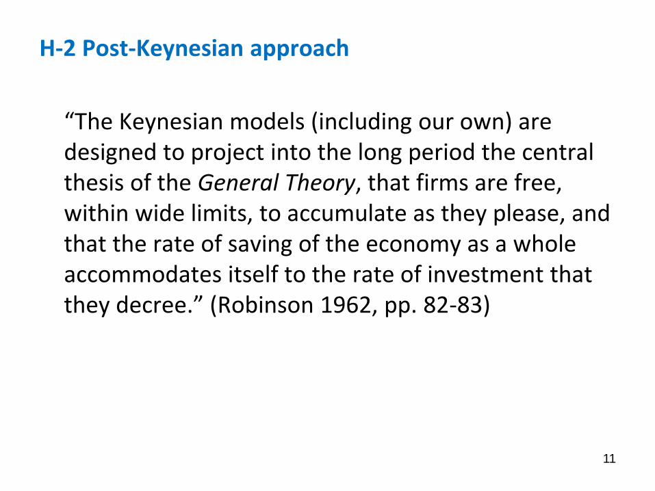
H-2 Post-Keynesian approach

“The Keynesian models (including our own) are designed to project into the long period the central thesis of the General Theory, that firms are free, within wide limits, to accumulate as they please, and that the rate of saving of the economy as a whole accommodates itself to the rate of investment that they decree.” (Robinson 1962, pp. 82-83)

12

• Capital accumulation is independent of saving, I S, no Say‘s law

• Harrod, Domar: Explore conditions for balanced growth, Harrod detects instability of ‚warranted rate of growth‘

• Kaldor, Pasinetti, Robinson: Capital accumulation (and hence growth) determines the rate of profit and thus income distribution in the long run: r = g/sΠ

• Kalecki, Steindl: Capital accumulation determines growth and the degree of utilisation of productive capacities, as well as the rate of profit; distribution is determined mainly by mark-up pricing in incompletely competitive markets.

• Endogenous growth models driven by effective demand, i.e. productivity growth is also demand determined

13

Model comparison by means of different closures

• closed one good economy without a government

• two classes: workers and capitalists

• workers receive wages and don’t save

• capitalists own MoP and receive profits which are partly consumed partly saved

• no depreciations

• no overhead labour

14

Rate of profit:

(1) v

1hu

K

Y

Y

Y

pYpKr

p

p

r: rate of profit, : profits, p: price, K: capital stock, Y: output,

Yp: potential output, h: profit share, u: rate of capacity utilisation,

v: capital-potential output ration

Saving rate:

(2) 1s0,v

1husrs

pK

s

pK

S

: saving rate, S: saving, s: propensity to save out of profits

15

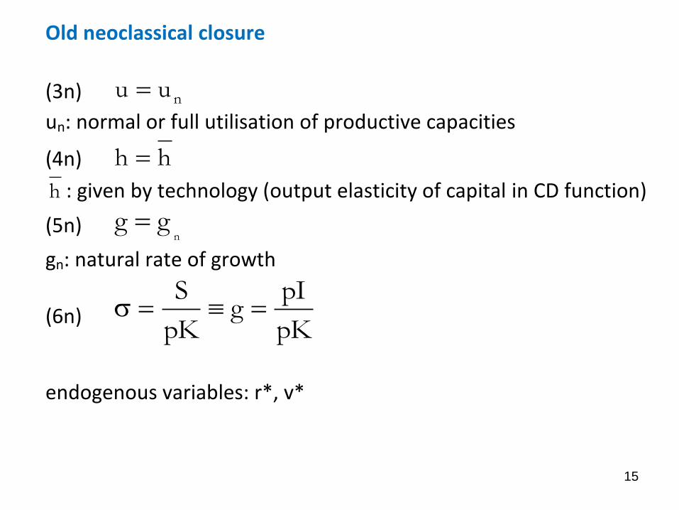
Old neoclassical closure

(3n) nuu

un: normal or full utilisation of productive capacities

(4n) hh

h : given by technology (output elasticity of capital in CD function)

(5n) n

gg

gn: natural rate of growth

(6n) pK

pIg

pK

S

endogenous variables: r*, v*

16

Figure 1: The old neoclassical distribution and growth model

r

v

g = =sr

g,

r=hun/v

v*

r*

g*= gn

17

Table 2: Effects of changes in exogenous variables on endogenous variables in the

old neoclassical growth model

Exogenous

variables

Endogenous variables

*g r* v*

gn + + –

s 0 – +

h 0 0 +

un 0 0 +

18

New neoclassical growth theory closure

(3ng) nuu

un: normal or full utilisation of productive capacities

(4ng) hh

h : given by technology

(5ng) A

1v

A: constant productivity of capital (AK model: Y = AK)

(6ng) pK

pIg

pK

S

endogenous variables: r*, g*

19

Figure 2: The new neoclassical growth theory

r

v

g = =sr

g,

r=hun/v

v = 1/A

r*

g*

20


new neoclassical growth theory

Exogenous

variables


*g r*

v – –

h + +

un + +

s + 0

21

Classical/Marxian closure

(3cm) nuu

(4cm) aw1aw1pY

wLpYh r

s

r

w: nominal wage rate, wr: real wage,

wrs: conventional/subsistence real wage rate,

L: labour, a: labour-output ratio

(5cm) vv

(6cm) pK

pIg

pK

S

Endogenous variables: r*, g*

22

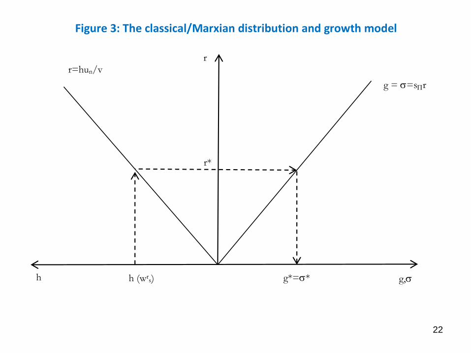
Figure 3: The classical/Marxian distribution and growth model

r

h

g = =sr

g,

r=hun/v

h (wrs)

r*

g*=*

23


classical/Marxian distribution and growth theory

Exogenous

variables


*g r*

h + +

un + +

v – –

s + 0

24

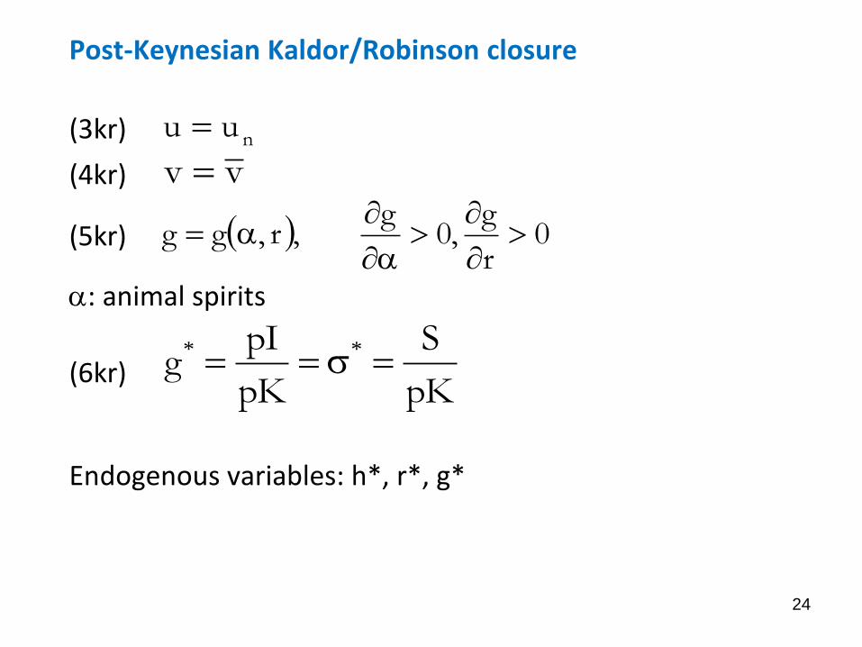
Post-Keynesian Kaldor/Robinson closure

(3kr) nuu

(4kr) vv

(5kr) 0r

g,0

g,r,gg

: animal spirits

(6kr) pK

S

pK

pIg **

Endogenous variables: h*, r*, g*

25

Figure 4: The Kaldorian/Robinsonian post-Keynesian distribution and growth model

r

h

=sr

g,

g(,r) r=hun/v

h*

r*

g*=*

26


post-Keynesian Kaldor-Robinson distribution and growth model

Exogenous

variables


*g* r* h*

+ + +

g/r + + +

s – – –

v 0 0 +

un 0 0 –

27

Post-Keynesian Kalecki/Steindl closure

(3ks) 0,

m

hmhh

m: mark-up

(4ks) vv

(5ks) 0,0,0,0,,,,

v

g

u

g

h

ggvuhgg

(6ks) pK

S

pK

pIg **

Endogenous variables: u*, r*, g*

28

Figure 5: The Kaleckian/Steindlian post-Keynesian distribution and growth model

r

u

=sr

g,

g(,u,h,v) r=uh(m)/v

u*

r*

g*=*

29


post-Keynesian Kalecki-Steindl growth theory

Exogenous

variables


*g* r* u*

+ + +

g/u + + +

g/h + + +

s – – –

v 0 0 +

h –/+ –/+ –/+

30

Figure 6: A reduction in the profit share in the Kalecki-Steindl growth theory: the neo-

Kaleckian model and the wage-led demand/wage-led growth regime of the post-Kaleckian

model

r

u

=sr

g,

g(,u,h,v)

r=uh(m)/v

u*

r*

g*=*

31

Figure 7: A reduction in the profit share in the Kalecki-Steindl growth theory: the

intermediate case with wage-led demand and profit-led growth in the post-Kaleckian

model

r

u

=sr

g,

g(,u,h,v)

r=uh(m)/v

u*

r*

g*=*

32

1

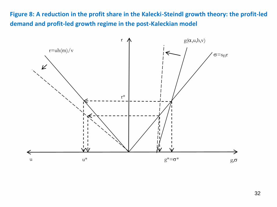
Figure 8: A reduction in the profit share in the Kalecki-Steindl growth theory: the profit-led

demand and profit-led growth regime in the post-Kaleckian model

r

u

=sr

g,

g(,u,h,v)

r=uh(m)/v

u*

r*

g*=*

33






34

Assumptions • Open economy without government

• Imported raw materials

• Output competes in international markets

• Prices of imported inputs and competing foreign output are given

• Nominal exchange rate is given, determined by monetary policies

and financial markets

• Foreign economic activity is given

A post-Kaleckian open economy model with saving out of wages Hein/Vogel (2008) and Hein (2014, Chapter 7.3)

35

(19)

(20)

(21)

.

p prices

pf foreign prices

m mark-up

w nominal wage rate

a labour coefficient

e nominal exchange rate

μ unit material inputs

z relationship between unit material costs and unit labour costs

fp 1 m wa p e , m 0

fp ez

wa

fp ep 1 m wa 1 1 m wa 1 z

wa

mark-up pricing on constant unit variable costs

relationship between unit material and unit labour costs

Prices depend on mark-up, unit labour costs, and relationship between unit material and unit labour costs

7.3.1 Prices, distribution and international competitiveness

36

(23)

(24)

. .

(22)

h profit share

Π profits

W wages

er real exchange rate

mwa 1 z m 1 z 1h

1W mwa 1 z wa 1 m 1 z 11 z m

p

epe f

r

ppee fr

Profit share depends on mark-up and on the relationship between material and labour costs

International price competitiveness is given by real exchange rate

Rising real exchange rate implies increasing price competiveness

37

.

(23b)

(23a)

f fr

2

ep wa p ee0

m p

fr

2

ep 1 m ae0

w p

(23c)

0

p

p

epm1p

p

pm1eppp

e

e

f

2

f

2

fffr

Increasing profit share caused by an increasing mark-up implies falling competiveness

Increasing profit share caused by falling nominal wages implies increasing competiveness

Increasing profit share caused by nominal depreciation of domestic currency implies increasing competiveness

38

(25)

.

rr r

r

ee e (h), 0 , if dz 0 and dm 0 ,

h

e0, if dz 0 and dm 0.

h

Increasing profit share caused by an increasing mark-up falling competitiveness Increasing profit share caused by falling nominal wages: increasing competitiveness Increasing profit share caused by nominal depreciation: increasing competitiveness

39

7.3.2 Distribution and growth

(26) NXIMeppXpISf

.

(27) bg .

(28) .1ss0,v

uhsss

pK

)Y(ss

pK

SSWWW

WW

(29) 0,,hug .

(30) 0,,,uu)h(ebf

r .

(31) .0v

1hsss0

u

b

u

g

uWW

40

(32)

v

1hsss

u)h(ehu

WW

f

r* ,

(33)

v

1hsss

uhev

1hsssh

g

WW

f

r

WW* ,

(34)

v

1hsss

u)h(ehv

h

r

WW

f

r

* ,

(35)

v

1hsss

hv

1hsssuhe

b

WW

WWf

r

* .

41

(32c)

v

1hsss

h

e

v

uss

h

u

WW

r

W*

,

(33c)

v

1hsss

h

e

v

uss

v

1hsss

h

g

WW

r

WWW*

.

(32c’) 0h

e

v

uss:if,0

h

u r

W

*

.

(33c’)

0

h

e

v

ussv

1hsss

:if,0h

g r

W

WW*

.

42

Table 2

Demand and accumulation/growth regimes in an open economy post-Kaleckian distribution and growth model with positive saving out of wages

h

u *

h

g *

Wage-led regime Wage-led (stagnationist) demand and wage-led accumulation/growth:

0h

e

v

ussv

1hsss

h

e

v

uss

r

W

WWr

W

– –

Intermediate regime Wage-led (stagnationist) demand and profit-led accumulation/growth:

h

e

v

ussv

1hsss

0h

e

v

uss

r

W

WWr

W

– +

Profi-led regime Profit-led (exhilarationist) demand and profit-led accumulation/growth:

h

e

v

ussv

1hsss

h

e

v

uss0

r

W

WWr

W

+ +

43

Implications for wage and exchange rate policies

• Aggressive wage policies will be successful in rasing the wage share, even with a constant mark-up.

• In a wage-led economy this will have expansionary effects on domestic demand. However, net exports are affected in the negative, so that the overall effects need not be positive.

• In a profit-led domestic economy, overall negative effects will emerge.

• Nominal wage moderation or nominal depreciation will be expanionary in a domestic profit-led regime.

• But if the domestic regime is wage-led, the overall effects are uncertain: wage moderation or nominal depreciation will stimulate net exports, but the associated redistribution in favour of profits will have depressing effects on domestic demand in a wage-led economy. The overall effects may hence be negative.

Generally: An overall wage-led regime becomes less likely in an open economy setting.

44

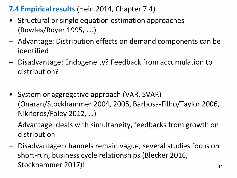
7.4 Empirical results (Hein 2014, Chapter 7.4)

• Structural or single equation estimation approaches (Bowles/Boyer 1995, ….)

Advantage: Distribution effects on demand components can be identified

Disadvantage: Endogeneity? Feedback from accumulation to distribution?

• System or aggregative approach (VAR, SVAR) (Onaran/Stockhammer 2004, 2005, Barbosa-Filho/Taylor 2006, Nikiforos/Foley 2012, …)

Advantage: deals with simultaneity, feedbacks from growth on distribution

Disadvantage: channels remain vague, several studies focus on short-run, business cycle relationships (Blecker 2016, Stockhammer 2017)!

45

Single equation estimations

(36) r

NX

r

I

* GZ,h,YNXZ,h,YIh,YCY .

Total differentiation of equation (36) yields:

(37) dhh

NXdY

Y

NXdh

h

IdI

Y

Idh

h

CdY

Y

CdY

rr*

.

Rearranging and collecting terms gives:

(38)

h

NX

h

I

h

C

x1

1

Y

NX

Y

I

Y

C1

h

NX

h

I

h

C

dh

dY r

r

r

*

,

with YNXYIYCx r .

If the feedbacks of changes in the level of aggregate demand and income on consumption,

investment and net exports, and hence the multiplier [1/(1-x)], are ignored, equation (38)

simplifies to:

(39) h

NX

h

I

h

C

dh

dY r

.

Dividing by Y gives the percentage change of aggregate demand caused by a one percentage

point change in the profit share:

(40) h

Y

NX

h

Y

I

h

Y

C

dh

Y

dY r

.

46

0h/YIh/YC domestic demand is profit led,

0h/YIh/YC domestic demand is wage led.

0dh/YdY , total demand is profit led,

0dh/YdY total demand is wage led.

47 Hartwig (2014), panel, OECD countries, 1971-2011, DD: W, TD: W

48

Table 4

Effect of a one percentage point increase in the profit share on private excess

demand and its components

h

Y

C

h

Y

I

h

Y

NX r

dh

Y

dY

A B C A+ B+ C = D

Euro area-12 -0.439 0.299 0.057 -0.084

Germany -0.501 0.376 0.096 -0.029

France -0.305 0.088 0.198 -0.020

Italy -0.356 0.130 0.126 -0.100

United

Kingdom

-0.303 0.120 0.158 -0.025

United States -0.426 0.000 0.037 -0.388

Japan -0.353 0.284 0.055 -0.014

Canada -0.326 0.182 0.266 0.122

Australia -0.256 0.174 0.272 0.190

Turkey -0.491 0.000 0.283 -0.208

Mexico -0.438 0.153 0.381 0.096

Korea -0.422 0.000 0.359 -0.063

Argentina -0.153 0.015 0.192 0.054

China -0.412 0.000 1.986 1.574

India -0.291 0.000 0.310 0.018

South Africa -0.145 0.129 0.506 0.490 Source: Onaran/Galanis (2012, Table 11)

49

Table 5

Summary of the multiplier effects at the national and global level

The effect of a 1

percentage-point

increase in the

profit share in only

one country on

private excess

demand

The effect of a 1

percentage-point

increase in the

profit share in only

one country on

percentage change

in equilibrium

aggregate demand

The effect of a

simultaneous

percentage-point

increase on

percentage change

in equilibrium

aggregate demand

D E F

Euro area-12 -0.084 -0.133 -0.245

United Kingdom -0.025 -0.030 -0.214

United States -0.388 -0.808 -0.921

Japan -0.014 -0.034 -0.179

Canada 0.122 0.148 -0.269

Australia 0.190 0.268 0.172

Turkey -0.208 -0.459 -0.717

Mexico 0.096 0.106 -0.111

Korea -0.063 -0.115 -0.864

Argentina 0.054 0.075 -0.103

China 1.574 1.932 1.115

India 0.018 0.040 -0.027

South Africa 0.490 0.729 0.390 Source: Onaran/Galanis (2012, Table 13)

50

7.5 Conclusions

• Pursuing a strategy of profit-led growth via the net export channel by relying on a kind of ‘beggar thy neighbour’ policy, may be a successful way for small open economies (f.e. Austria, Netherlands) in isolation.

• However, it cannot work for medium-sized and large open economies because it will reduce aggregate demand in these economies, and it will also harm the countries‘ trading partners (see: Germany in the EMU!) and, thus finally, the world economy as a whole. This will feed back on net exports of profit-led economies.

• For medium-sized and large open economies, as Germany, economic policy strategies have to take into account wage-led nature of aggregate demand. Same is true for the world as a whole

• Effects of re-distribution on aggregated demand are small re-distribution policies should be embedded into expansionary monetary and fiscal policies (Global Keynesian New Deal, Hein/Truger 2012/13); policy mix of incomes and fiscal policies (Onaran 2016)

51






Integrated analysis of money, finance and distribution and growth

(Hein 2014, Chapters 9-10) • Rate of interest as a monetary phenomenon, exogenous for

income generation and growth (Pasinetti 1974, p.47)

• Interest rate and functional income distribution (interest-elastic mark-up and profit share)

• Interest, finance and investment: Kalecki’s (1937) ‘principle of increasing risk’, Steindl’s (1952) ‘gearing ratio’, Minsky’s (1975, 1986) distinction between ‘hedge’, ‘speculative’ and ‘Ponzi’ finance

• Interest, debt and consumption (credit availability, wealth, relative income hypothesis, …)

Demand-driven small-scale analytical models

Large-scale, stock-flow consistent (SFC) models in the tradition of Godley (Cambridge) and Tobin (Yale) (Godley/Lavoie 2007) 52

The integration of interest and credit into post-Keynesian distribution and growth models

• Since the late 1980s/early 1990s, several attempts at integrating monetary variables into different types of post-Keynesian distribution and growth models

• Three classes (rentiers, managers/firms, workers); interest and debt of firms affect income distribution, investment and consumption through the income shares of the three groups; demand, growth and (financial) stability

Steindl’s macroeconomic paradox of debt (Dutt 1995), debt-led (Minskyian) and debt-burdened (Steindlian) regimes (Taylor 2008)

‘Normal’, ‘intermediate’ and ‘puzzling’ cases for effects of interest rate/debt changes (Lavoie 1995)

Only ‘debt-led’ and ‘puzzling’ regimes seem to be stable (Hein 2007)

Further debate on stability: Sasaki/Fujita (2012), Hein (2013), Franke (2016)

Including Minsky: Charles (2008a; 2008b; 2008c), Lima/Meirelles (2007), Meirelles/Lima (2006), Nishi (2012b), Ryoo (2013)

53

Financialisation in post-Keynesian distribution and growth models

• Since the early/mid-2000s, post-Keynesian have increasingly applied their integrated distribution and growth models to the ‘macroeconomics of finance-dominated capitalism (Hein 2012b)

• Channels: distribution, investment, consumption, current/capital account

Potential regimes: ‘Finance-led growth’ (Boyer 2000), ‘profits without investment’ (Cordonnier 2006), ‘contractive’; only the former seems to be (financially) stable in the long run.

• Empirically, ‘profits without investment’ seems to have dominated:

‘Debt-led private demand boom’ vs. ‘export-led mercantilist’ regimes before the crisis with high instability potential each

• Alternative: Wage-led/mass income-led regime (Lavoie/Stockhammer 2013, Stockhammer/Onaran 2013) embedded in a Keynesian Deal (Hein/Mundt 2012, Hein/Truger 2011; 2012/13):

Re-regulation of finance, re-distribution of income, re-orientation of macro-policy, and re-creation of international policy coordination

54

55






Debates 1: Endogenous rate of capacity utilisation beyond the short run?

• Harrodian/Marxian critique (Dumenil/Levy 1999, Shaikh 2009, Skott 2010, 2012): Deviation of utilisation from normal rate is not consistent with long-run equilibrium; paradox of costs disappears.

Normal/optimal rate of in a world of uncertainty is a range (Dutt 1990, 2005a, 2010a)

Firms have multiple goals and accept deviations from target or normal rate or utilisation (Dallery/van Treeck 2010)

Firms’ assessment of trend growth and normal rate is endogenous to actual experience (Lavoie 1995a, 1996a)

Normal rate as stable inflation rate of utilisation is endogenous to monetary policies (Hein 2006a, 2008)

Autonomous expenditure growth driving the system allows for Kaleckian results regarding growth path even with normal rate of utilisation (Allain 2015, Lavoie 2016a, Nah/Lavoie 2017)

56

Debates 2: What about the feedback of demand/growth on distribution?

• Have Kaleckians ignored feedbacks of demand and growth on

income distribution (Skott 2016)?

Kaleckian models with feedbacks of demand, employment or growth on distribution: Assous/Dutt (2013), Bhaduri (2008), Blecker (2011), Cassetti (2003; 2006; 2012), Dutt (2006a; 2010b; 2012), Hein/Stockhammer (2010; 2011b), Lavoie (2010; 2014, Chapter 6), Stockhammer (2004), …

Feedback of demand and employment on distribution is not unique, applying Kalecki’s theory of distribution (Dutt 2012)

Feedback depends on changes in socio-institutional factors, in particular in the medium to long run

Income shares are thus taken to be exogenous when it comes to the analysis of medium-/long-run wage vs. profi-led demand/growth

57

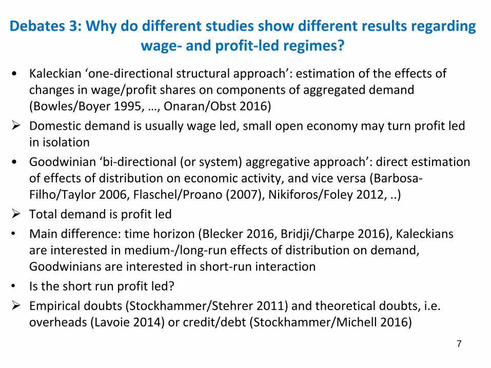
Debates 3: Why do different studies show different results regarding wage- and profit-led regimes?

• Kaleckian ‘one-directional structural approach’: estimation of the effects of

changes in wage/profit shares on components of aggregated demand (Bowles/Boyer 1995, …, Onaran/Obst 2016)

Domestic demand is usually wage led, small open economy may turn profit led in isolation

• Goodwinian ‘bi-directional (or system) aggregative approach’: direct estimation of effects of distribution on economic activity, and vice versa (Barbosa-Filho/Taylor 2006, Flaschel/Proano (2007), Nikiforos/Foley 2012, ..)

Total demand is profit led

• Main difference: time horizon (Blecker 2016, Bridji/Charpe 2016), Kaleckians are interested in medium-/long-run effects of distribution on demand, Goodwinians are interested in short-run interaction

• Is the short run profit led?

Empirical doubts (Stockhammer/Stehrer 2011) and theoretical doubts, i.e. overheads (Lavoie 2014) or credit/debt (Stockhammer/Michell 2016)

7

Debates 4: Are functional income distribution and the wage-led vs. profit-led distinction still relevant with rising personal income

inequality and household debt? • Falling wage shares and rising inequality, but rising instead of falling private

consumption in countries like US before crisis

Debt in workers’ consumption function (Dutt 2005b, 2006b, Hein 2012a, Nishi 2012a, …)

wealth and debt effects on consumption (Bhaduri/Laski/Riese 2006, Bhaduri 2011a, 2011b, …);

relative income hypothesis (Belabed/Theobald/van Treeck 2013, Carvalho/Rezai 2016, Kapeller/Schütz 2014, 2015, Kim/Setterfield/Mei 2014, …)

Empirical results regarding relative income hypothesis are inconclusive; financial and residential wealth, as well as debt effects on consumption for some countries quite robust.

Wage share is still important, because household debt can only temporarily boost consumption without triggering financial instability, but personal distribution and wage dispersion matters – irrespective of wage- or profit-led demand (Palley 2016)

59

60

Appendix

• Stagnation tendencies seen from a

Steindlian/Kaleckian perspective

A Steindlian model of growth and stagnation

based on Steindl (1952, Chapter XIII), reformulations by Dutt (1995, 2005), Flaschel/Skott (2006)

here: simplification by Hein (2016)

Assumptions:

• Closed private one-good economy

• Fixed coefficients production technology

• No overhead labour, no depreciation

• Harrod-neutral technological change

• Three classes: rentiers, managers/capitalists, workers

• No labour supply constraint

• Mark-up pricing in oligopolistic markets

61

62

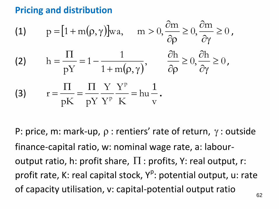
Pricing and distribution

(1) 0m

,0m

,0m,wa,m1p

,

(2)

0h

,0h

,,m1

11

pYh

,

(3) v

huK

Y

Y

Y

pYpKr

p

p

1

.

P: price, m: mark-up, : rentiers’ rate of return, : outside

finance-capital ratio, w: nominal wage rate, a: labour-

output ratio, h: profit share, : profits, Y: real output, r:

profit rate, K: real capital stock, Yp: potential output, u: rate

of capacity utilisation, v: capital-potential output ratio

63

Financing of the capital stock and rentiers income

(4) FR EEBpK ,

(5) pK

EB R ,

(6) pK

EF ,

(7) RF ,

(8) BER R .

B: debt, ER: equity held by rentiers, EF: accumulated

retained earnings, : outside finance-capital ratio,

: inside finance-captital ratio, F : retained earnings,

R: rentiers‘ income, : rentiers‘ rate of return

64

Saving, investment and equilibrium

(9) 1s0,)s1(v

uh

pK

RsR

pK

SRR

R

.

(10) 1,0,,,v

uhuuy

pK

pIg 0

,

(11) g ,

(12) .0v

h10

u

g

u

: saving rate, S: saving, sR: propensity to save out of rentiers’ income,

g: accumulation rate, I: investment, : autonomous investment, animal

spirits, y : productivity growth, u0: target rate of utilisation.

65

Goods market equilibrium with exogenous technological progress:

(13)

v

h1

s1uyu R0* ,

(14)

v

h1

v

hss1

v

huy

gRR0

* ,

(15)

v

h1

v

hs1uy

rR0

* .

66

Responses of goods market equilibrium rates of capacity utilisation (u),

capital accumulation (g), profit (r) towards changes in exogenous

variables and parameters

u* g* r*

+ + +

y + + +

u0 – – –

sR – – –

h – – –

? ? ?

? ? ?

Endogenous technological progress and total equilibrium

• Kaldor’s (1957, 1961): technical progress function

• Kaldor’s (1966): Verdoorn’s Law

• Marx (1867), Hicks (1932): wage push

67

(16) 0,,,hgy .

(17)

0 R R**

hu h 1 s s

vg

h1

v

.

(18)

0 R R

**

h hh 1 u 1 s s

v vy

h1

v

.

68

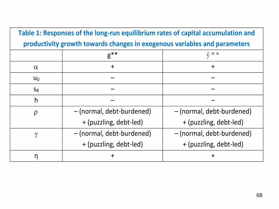
Table 1: Responses of the long-run equilibrium rates of capital accumulation and

productivity growth towards changes in exogenous variables and parameters

g** y * *

+ +

u0 – –

sR – –

h – –

– (normal, debt-burdened)

+ (puzzling, debt-led)







η + +

69

Figure 1: Stagnation with endogenous productivity growth

A

B

C

Stagnation policy or stagnation as a political trend

• decrease in autonomous government expenditure growth, reform policies causing falling animal spirits fall in

• lower public investment in R&D fall in η

• weakening workers’ and trade union bargaining power, higher interest rates and hence overhead costs rise in h

• rising inequality in the distribution of household incomes, higher uncertainty triggering precautionary saving rise in s

• a rise in the rentiers’ rate of return, hence the interest rate and/or the dividend rate, and/or the outside finance-capital ratio, hence the debt- and/or the rentiers’ equity-capital ratio, if the economy is in the ‘normal case’ and in a ‘debt-burdened’ regime

70

Steindlian anti-stagnation policies • stabilising and raising public autonomous expenditure growth, as well as

discretionary anti-cyclical fiscal policies,

• raising growth enhancing public investment, focusing on infrastructure, technology, education and R&D expenditures,

• stabilising and raising the wage share by full employment policies, improving workers’ bargaining power, by low interest rate policies, reducing overhead costs, and by the re-regulation of the financial sector reducing the power and income claims of rentiers and shareholders,

• lowering the households’ propensity to save by means of redistributing income, both pre-tax via higher wage shares and a more compressed wage structure and after-tax by progressive taxation and social transfers, as well as by removing uncertainty triggering precautionary saving,

• improving international economic and monetary policy coordination in order to avoid severe current account imbalances, ‘beggar thy neighbour’ strategies, on the one hand, and rising indebtedness in foreign currencies, on the other hand.

71

distribution and growth - hans-böckler-stiftung - … · on equilibrium growth rate ......

Documents