corruption, income distribution, and growth

CEMA Working Paper No. 472

Corruption, Income Distribution, and Growth

Hongyi Li, Lixin Colin Xu, Heng-fu Zou*

Abstract. This paper uses an encompassing framework developed by Murphy et al. (1991,

1993) to study corruption and how it affects income distribution and growth. We find that

(1) corruption affects income distribution in an inverted U-shaped way, (2) corruption

alone also explains a large proportion of the Gini differential across developing and

industrial countries, and (3) that even after correcting for measurement errors, corruption

still retards economic growth. But the effect is far less pronounced than the one found in

Mauro (1995). Moreover, corruption alone explains little of the continental growth

differentials. In countries where the asset distribution is less equal, corruption is associated

with a smaller increase in income inequality and a larger drop in growth rates.

Key Words: Corruption; income inequality; economic growth.

JEL: D3, K4, and O4.

* Hongyi Li is at the Chinese University of Hong Kong; Lixin Colin Xu and Heng-fu Zou are both at the World Bank and the latter also affiliated with Peking University. We thank Robert Cull and Raymond Fisman for comments. We are also grateful for the comments of two referees, which led to a substantial revision of the paper. The findings, interpretations, and conclusions expressed in this paper are entirely those of the authors. They do not necessarily represent the views of the World Bank. Mailing Address: Dr. Heng-fu Zou, The World Bank, MC2-611, 1818 H St, NW, Washington, DC, 20433, USA. Email: [email protected].

1


I. INTRODUCTION

The literature defines corruption as an illegal payment to a public agent to obtain a

benefit that may or may not be deserved, or, the abuse of public offices for private gains

[Rose-Ackerman (1978, 1996), Klitgaard (1988), Shleifer and Vishny (1993)]. In the real

world, corruption probably amounts to a large share of the gross national product in

countries like Zaire and Kenya [Shleifer and Vishny (1993)]. Corruption worries policy

makers and international organizations, who remain adamant about the adverse effects of

corruption; the academic literature is less definite about how corruption influences growth

and inequality.1

Many scholars are not overly concerned about corruption. Leff (1964), for example,

views corruption as “grease money” to lubricate the squeaky wheels of a rigid

administration. Francis T. Lui (1985) shows how bribes minimize the waiting costs

associated with queuing therefore reducing the inefficiency in public administration in a

Nash equilibrium. Both of these models equate bribes as allocating the true worth of the

underlying favor, licenses, or permit to the most worthy bidder. Forbidding bribes then

amounts to prohibiting the use of price mechanism in the public sector. It is perhaps this

view that prompted the famous political scientist, Huntington (1968, p. 386), to write: "In

terms of economic growth, the only thing worse than a society with a rigid, over-

centralized, dishonest bureaucracy is one with a rigid, over-centralized, honest

bureaucracy."

Much of the recent literature, however, views corruption as much more than a price

mechanism. Corruption, after all, imposes an extortionary tax [Murphy, Shleifer, and

1 For a comprehensive review of issues related to corruption, see Bardhan (1995).

2


Vishny (1991); Mauro (1995)]. Furthermore, the need for secrecy may distort investment

projects toward those offering better opportunities for corruption, such as defense and

infrastructure, for which it is harder to measure performance and quality [Shleifer and

Vishny (1993)]. In addition, once corruption becomes endogenized in the general

equilibrium setup, bribing may no longer be akin to bidding for scarce resources. Corrupt

officials may intentionally delay the queuing process to extract more bribes [Myrdal,

(1968)], perhaps partly because corruption contracts are not enforceable in courts [Shleifer

and Vishny (1993)]. Corruption may also cause misallocation of talents. Because

corruption represents a higher return to rent-seekers, talent flows out of the innovation

sector to the rent-seeking sector. In so far as the pace of technological progress is

determined by the talent pool of the innovation sector, growth rates drop in societies in

which corruption is widespread [Murphy, Shleifer, and Vishny (1991)]. Finally,

innovators or entrepreneurs are hit hardest by corruption as they must obtain government-

supplied goods such as licenses and permits to start, whereas established producers do not

[Murphy, Shleifer, and Vishny (1993)].

The empirical literature on corruption gradually emerging in this decade suggests a

negative relationship between corruption and growth. Mauro (1995), the first to look at

how corruption affects growth in a cross-country sample, concludes that corruption causes

slower growth. The main instrument for corruption in the growth equation, the

ethnolinguistic fracturization, however, has been shown to be a significant determinant of

growth, both directly and indirectly (through other policy variables) [Easterly and Levine

(1997)]. Thus it no longer serves as a valid instrument for corruption in the growth

regression. Using a cross-country sample, Murphy, Shleifer, and Vishny (1991) find that a

3


larger rent-seeking sector, as proxied by the ratio of college enrollments in law to total

college enrollments, is associated with a lower growth rate. Knack and Keefer (1995) find

that the quality of government institutions, including the degree of corruption, affects

investment and growth as much as other political economy variables (e.g., political

freedom, civil liberties, and political violence). Kaufman and Wei (1998) find that firms

that pay more bribes also spend more time with bureaucrats in more corrupt countries and

have a higher cost of capital, thus countering the view of corruption as "grease money."

Finally, transitional countries are likely to have a smaller unofficial economy where taxes

are fairer and regulation is less [Johnson, Kaufman, and Shleifer (1997)].

Even so, many questions about the impact of corruption remain unanswered. For

example, how does corruption affect income inequality? Since Mauro (1995) does not

correct for measurement error, one wonders whether corruption will still affect growth

adversely if more policy controls are added. In addition, capital market imperfection and

government spending have been suggested as two channels for corruption to affect

inequality and growth. Is this assertion empirically valid? Finally, to what extent can

corruption explain the differences in inequality and growth, say, between continents?

We examine these issues by looking at how corruption affects the Gini coefficient

and growth rates in a sample of countries, using the recently-compiled income distribution

data by Deninger and Squire (1996) and a corruption index published by Political Risk

Services. Using the theoretical framework developed by Murphy, Shleifer, and Vishny

(1991, 1993), we derive testable implications about how corruption affects inequality and

growth. Most of these implications are found to be empirically valid. In particular, we find

that corruption affects the Gini coefficient in an inverted U-shaped way; that is, inequality

4


is low when levels of corruption are high or low, but inequality is high when corruption is

intermediate. Corruption alone also explains a large proportion of the Gini differential

across continents.2 Even after correcting for measurement errors and imposing a rich

conditional information set, corruption still retards economic growth. Corruption, however,

does not explain much of the growth differentials across continents. In countries where

asset distribution is less equal, corruption is associated with a smaller increase in income

inequality and a larger drop in growth rates. Finally, corruption raises income inequality to

a lesser extent in countries with higher government spending.

The paper contributes to the empirical literature of corruption in five ways. First,

we modify the framework of Murphy, Shleifer, and Vishny (1991, 1993) to derive a rich

set of empirical implications about the effects of corruption on growth and income

distribution. Second, we examine, for the first time, the relationship between corruption

and income inequality. Third, we check the robustness of the relationship between growth

and corruption while dealing with measurement errors. Fourth, we allow the effects of

corruption to depend on government spending and measures of capital market imperfection.

And finally, we investigate the potential role of corruption in explaining the differences in

income inequality and growth rates across continents.

Section II presents a theoretical framework for examining how corruption affects

growth and inequality. Section III discusses our data and then presents evidence on the

effects of corruption. Section IV concludes.

2 Here we use "continent" in a loose way. We mean the comparison of Asia, Latin America, and OECD countries.

5


II. CORRUPTION, INCOME DISTRIBUTION AND GROWTH: AN

ANALYTICAL FRAMEWORK

Murphy, Shleifer, and Vishny (1991, 1993) offer an encompassing framework to

discuss how corruption affects both inequality and growth. In this section we modify their

models, especially the model in the second paper, to make the effects of corruption on

inequality and growth more transparent.

A resident in a country can produce in either the traditional or the modern sector. In

the traditional sector she produces , and in the modern sector she produces , with > .

The technological progress in the traditional sector is assumed to be slower than the

modern sector. To simplify, we normalize the growth rate of the traditional sector as zero,

and that of the modern sector as g, with g > 0. We assume that g decreases as the tax rate

goes up in the modern sector. The advantage of the traditional sector is that it is not subject

to expropriation, while the modern sector is. The reason is that entrepreneurs in the modern

sector must obtain permits, licenses, and import quota from the government and are

vulnerable to effects of corruption and rent-seeking behavior.

When not in productive sectors, one can also be a rent-seeker. Rent-seeking is

characterized by a constant-return-to-scale technology of appropriating: the maximum

amount one can appropriate is . Let the ratio of people in the rent-seeking sector to the

modern sector be n. Then the return to the modern sector will be ( - n). Assuming that

people maximize income, the allocation of labor across sectors will depend on , , and .

The allocation in turn affects the average income level, income distribution, and growth

rates. We analyze three cases.

1. < . This corresponds to a non-corrupt society that protects property rights.

6


With a low return on rent-seeking, everybody specializes in the modern sector. As a

consequence, the average income at time t is egt, the highest amount possible, and the

growth rate is g. The Gini coefficient is zero.

2. > . This is an extremely corrupt society that does not protect property rights.

Since the return to rent-seeking is higher than any alternative activity, many people choose

to be rent-seekers. Eventually, as the number of rent-seekers rises, the productivity of the

modern sector falls to that of the traditional sector, i.e., - n = . Call this threshold ,

then n = ( - ) / . Since = at n , which is the interception for the return curves of

the modern sector, the traditional sector, and the rent-seeking activity, n = / - 1. In this

economy, then, the average income level is , the lower bound of individual earning in the

population. The Gini coefficient is zero. The growth rate is between 0 and g because some

people are in the modern sector.

n'

' '

'

3

3. < < . This corresponds to an intermediate level of corruption. There are

three equilibria: (i) the good equilibrium as in case 1 where everybody is in the modern

sector; (ii) the bad equilibrium as in case 2, where people work in the modern, traditional,

and rent-seeking sector, with equilibrium n = / - 1; and (iii) people work only in the

modern and the rent-seeking sectors, and the return to the modern sector is equated to that

of rent-seeking, i.e., - = , where is the equilibrium ratio of rent-seekers to

workers in the modern sector. Then n = / -1 < n . Therefore, fewer people specialize

n' ' n' '

' ' '

3 The exact number of people in the traditional and the modern sector is indeterminate here, only the ratio n is determinate. The indeterminacy could be eliminated if there is decreasing returns to scale to production, which is an unnecessary complication here.

7


in rent-seeking than in the equilibrium in case 2.4 The income level is , higher than that in

case 2 but lower than that in case 1. Since fewer people choose to be rent-seekers and more

people opt to work in the modern sector than in case 2, the growth rate g is larger.

Similarly, the growth rate is lower than that in case 1, the good equilibrium.

It is conceivable that all three types of equilibria coexist in countries with an

intermediate level of corruption. The variation in incomes (as measured by the coefficient

of variation of incomes) in these countries, then, is higher than in countries with either

high or low corruption (cases 1 and 2)—in cases 1 and 2, the equilibrium incomes are

more likely to be similar. Moreover, the average income level and grow rate should be

bounded by those of cases 1 and 2.

Now we summarize the main empirical implications from the model, and when

appropriate, discuss further implications from the literature about how corruption affects

inequality and growth:

Corruption affects inequality in an inverted U-shaped way: Inequality in countries with

an intermediate level of corruption is higher than that in countries with little or rampant

corruption.

Corruption should be negatively correlated with the income level.

Corruption should also be negatively correlated with growth. This conclusion is

reinforced by elements not considered in the model. In Murphy, Shleifer, and Vishny

(1991), for instance, corruption is viewed as a tax on the profits from the productive

4 Implicitly we assume that the higher the ratio of rent-seekers to modern-sector workers, the higher the number of rent-seekers. This may not be true because, as pointed out in footnote 3, only the ratio is determined in the equilibrium, not the numbers. However, once we introduce decreasing returns to scale to production, the allocation of labor between the modern and the traditional sector will become determinant, and our implicit assumption holds.

8


sector. According to this logic, an increase in corruption amounts to a tax hike, which

pulls talented entrepreneurs toward the rent-seeking sector; growth rates, in turn, drop.

In addition, bureaucrats may distort investment toward projects offering better

opportunities for secret corruption, such as defense and infrastructure [Shleifer and

Vishny, (1993)]. The distortion in the composition of the modern sector raises the

relative return to rent-seeking activity and, as a result, growth rates and income levels

drop.

There are further implications based on the above framework that are not modeled

explicitly.

(i) Since corruption pulls labor to the traditional sector--which needs low-skilled

workers--the demand for unskilled relative to skilled workers increases. As a result,

population growth in more corrupt countries will be higher.

(ii) In so far as the modern sector is likely to be concentrated in cities, and corruption

discourages the modern sector, countries with more corruption are likely to be less

urbanized.

(iii) Corruption affects reliance on banks or other financial intermediaries for business

transaction. Johnson, Kaufman, and Shleifer (1997), for instance, note that fairer

taxation and fewer regulations are associated with smaller unofficial economies in

transitional economies of Eastern Europe and the Former Soviet Union. We thus

expect a more corrupt country to experience a lower level of financial deepening.

An important variable related to corruption is the share of government spending. A

larger share of government spending, financed by higher taxes on the modern sector,

reduces investment rates, discourages talented people from becoming entrepreneurs,

9


thus reduces growth rates (Murphy, Shleifer, and Vishny, 1991). We therefore expect

corruption in countries with higher government spending to have slower growth.

Furthermore, a heavier tax for the modern/entrepreneur sector reduces the income

differential between the modern and the traditional sector. We thus expect the effects

of corruption in raising income inequality to be smaller in countries with more

government spending.

Assume that a high land Gini coefficient implies credit constraints for entry into the

modern sector or becoming an entrepreneur (Li, Squire, and Zou, 1998)—without

assets as collateral, one has difficulties obtaining startup capital. A high land Gini

coefficient then should be associated with a larger traditional sector. Since corruption

mainly taxes the modern sector, corruption affects a smaller segment of the population

in a country with a larger traditional sector, and thus has a smaller impact on inequality.

We thus expect corruption to raise inequality to a lesser extent in countries with a

higher initial land Gini coefficient.5 Meanwhile, since a high land Gini coefficient

implies a large traditional sector and less talent pouring into the modern sector, this

results in a lower growth rate.

III. CORRUPTION, INCOME DISTRIBUTION, AND GROWTH: EVIDENCE

A. DATA

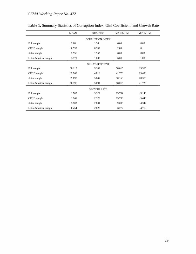
The corruption index and other institutional variables--available for 1982-1994--are

based on the data published by Political Risk Services/IRIS [see Knack and Keefer (1995)].

5 This claim is demonstrated heuristically in Appendix A.

10


The data set contains five related variables: corruption (CR), government repudiation of

contract (GRC), risk of expropriation (RSKE), rule of law (ROLAW), and bureaucratic

quality (BQ). For the summary statistics of the corruption index, see Table 1. Since the

five indices are highly correlated to each other (see Table 2), our regression analysis

focuses on the corruption index, which ranks between 0 (most corrupted) and 6 (least

corrupted). To make interpretation easier, the corruption index is transformed to (6 - the

index); still ranking between 0 and 6, now a larger index means a higher degree of

corruption.6

[ Tables 1 and 2 about here ]

The income inequality data are based on a new data set on the Gini coefficient

developed by Deininger and Squire (1996), which is widely regarded as having the best

inequality measure. Three criteria are used to compile the data. First, all observations are

based on national household surveys for expenditure or income. Second, coverage

represents the national population. Third, all sources of income and uses of expenditure are

accounted for, including own-consumption. Since the definition of the Gini coefficient

varies across countries in our sample--inequality can be measured by gross income, net

income, or expenditure, and it can be based on per capita or per household figures--proper

adjustment is necessary. We have adjusted the data following the procedure recommended

by Deininger and Squire (1996).7

6 Our measure of corruption is more updated and extensive than Mauro (1995). We cover the period 1982-1994; Mauro covers only 1980-83. After deleting observations without good Gini data, we cover 48 countries, and Mauro (1995) covers 37. 7 Specifically, we adjust for differences between income-based and expenditure-based coefficients by increasing the latter by 6.6 points (based on a 100 point scale), the average difference observed by Deininger and Squire (1996).

11


The growth rate is calculated using the real per capital GDP (PPP adjusted) as in

Summers and Heston (1994). The countries included in the analysis are Australia, Belgium,

Bangladesh, Bulgaria, Brazil, Canada, Chile, Colombia, Costa Rica, the Czech Republic,

Germany, Denmark, Dominican Republic, Spain, Finland, France, United Kingdom, Hong

Kong, Honduras, Hungary, Indonesia, India, Iran, Italy, Jamaica, Japan, South Korea, Sri

Lanka, Mexico, Malaysia, Netherlands, Norway, New Zealand, Pakistan, Panama, the

Philippines, Poland, Portugal, Singapore, Sweden, Thailand, Trinidad/Tobago, Tunisia,

United States, Venezuela, and Yugoslavia. The time period covered is 1980 to 1992.8

Figure 1 plots the average Gini against the average corruption index for the 47

countries. The Gini coefficient is positively correlated with corruption: the correlation

coefficient is 0.462 and statistically significant (p value of 0.000). Note the inverted U-

shaped line representing the simple regression of the Gini coefficient onto corruption and

its square. Figure 2 plots the average growth rate against the average corruption index. The

correlation coefficient is –0.048 (p value of 0.574). Although insignificant, this correlation

is in line with the empirical finding of Mauro (1995) that corruption is negatively

associated with growth rates.

[Figures 1 and 2 about here.]

In our empirical analysis the variables are, as in many other empirical studies,

averaged over five-year periods [see, for instance, Deininger and Squire (1997), Li, Squire,

and Zou (1998)]. The use of five-year averages reduces short-run fluctuations and allows

us to focus on the structural relationships of interest. Most variables are complete, but the

Gini coefficient is often missing in more than one year of each of the five-year periods; the

8 Although the corruption data are available up to 1995, the rest of variables are available only up to 1992.

12


five-year average then is computed based on non-missing observations. This should not

represent a problem because the Gini coefficient is found to be relatively stable over time

[Li, Squire, and Zou (1998)].

Following recent empirics on economic growth [Barro (1991), Levine and Renelt

(1992), King and Levine (1993), Alesina and Rodrick (1994)], we also consider a list of

other control variables in our regression analysis: (i) the initial GDP level (INIGDP), (ii)

primary years of schooling (SCHOOL), (iii) financial development (FINANCE), defined as

the money supply M2 over GDP, (iv) openness (OPEN), defined as imports over GDP, (v)

terms-of-trade shocks (TOTSHOCK), defined as the difference of the change in export

price and the change in import price, (vi) black market premium (BMP), (vii) government

spending (GOVSPEND), defined as government spending over GDP, (viii) average arable

land (AREA), (ix) the urbanization ratio (URB), (x) the population growth rate

(POPGROWTH), and (xi) following Atkinson (1997), initial distribution of asset as

measured by the initial land Gini coefficient (INILANDGINI). Most of these variables are

obtained through the World Bank national accounts and Summers and Heston (1994). The

black market premium data are from the Barro and Lee (1994) data set. The primary years

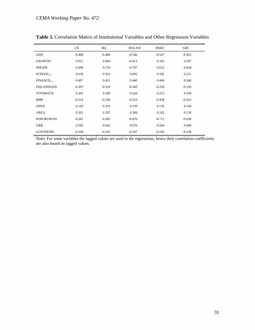
of schooling data are from Nehru et al. (1995). Table 3 provides the correlation

coefficients of the institutional variables and other regression variables based on the five-

year average data for the whole sample.

[Table 3 about here]

Next we investigate the relationship between income inequality and corruption as

well as the relationship between growth and corruption, while controlling for the effects of

initial GDP (for convergence effects), education (human capital investment), financial

13


development, and initial wealth distribution. Following Mauro (1995), Edwards (1997),

and Li, Squire, and Zou (1998), we estimate the following equations:

ititi

tiitit

ititi

tiitit

vIINILANDGINFINANCE

SCHOOLINIGDPCRGROWTH

uIINILANDGINFINANCE

SCHOOLINIGDPCRGINI

51,4

1,3210

51,4

1,3210

(1)

Here GINI is the Gini coefficient, GROWTH is the real per capita GDP growth. CR is the

corruption index. The country index is i, and the time index is t (t being 1, 2, and 3, the

time interval for 1980-84, 1985-89, and 1990-92). The lagged value of years of primary

schooling and the financial development index are used to account for possible

endogeneity.9 The initial GDP and the initial land Gini are of course time-invariant.

Since corruption is a subjective measure, it is likely to be badly measured. So for

each specification we correct for measurement errors. In particular, we use the average of

the corruption measure for each country in Mauro (1995)—which is time-invariant—and

its polynomials as instruments for our corruption measure. Since the Mauro measure

comes from different sources and covers an earlier period (1980-83), we do not expect the

measurement errors of the two proxies to be correlated. Since they are closely correlated,

the Mauro measure serves as a good instrument for our corruption measure [Greene (1997),

p.443].

B. CORRUPTION AND INCOME DISTRIBUTION

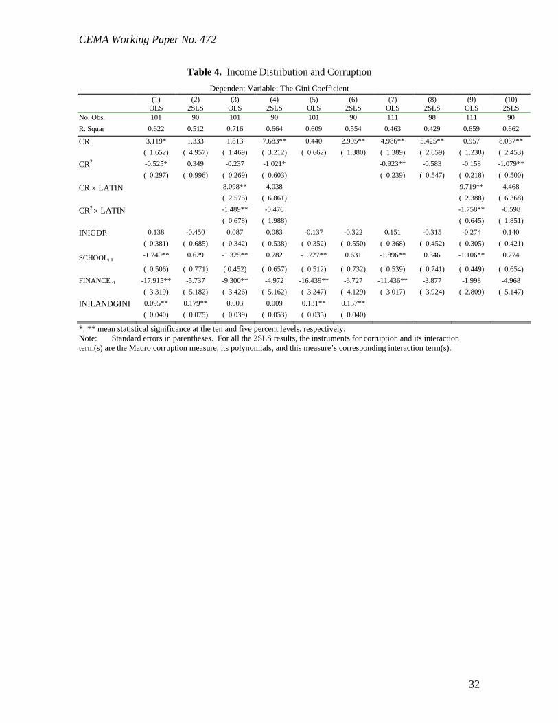
In the baseline regressions for the Gini coefficient (columns 1 and 2, Table 4),

corruption raises the Gini in an inverted U-shaped way. This is consistent with the

14


predictions of the model. The OLS results suggest that corruption begins to reduce the Gini

when the index exceeds 2.91. Although the 2SLS results do not preserve the quadratic

pattern of the OLS, as we shall see later, this pattern is robust to most other specifications.

Thus, consistent with our model, high or low levels of corruption are associated with low

inequality, while an intermediate level of corruption is associated with high income

inequality.

[ Table 4 about here ]

To examine the effects of corruption on income inequality across continents, we

experimented with alternative coefficients for each continent (columns 3 and 4, Table 4). It

turned out that only Latin American countries differ. Corruption affects the Gini

coefficient, again, in a quadratic way, both in the OLS and the 2SLS specification. Relative

to elsewhere, corruption in Latin American countries increases inequality to a larger

extent at low levels of corruption, and the implied marginal effects of corruption on

inequality drop faster as corruption increases.

What happens when the square of the corruption index is dropped? Corruption in

the OLS specification is no longer significant (columns 5 and 6 in Table 4). Taking

measurement errors into account, the 2SLS results—using an alternative measure of

corruption (the Mauro measure) and its polynomials as instruments—indicate that

corruption increases income inequality significantly. A one-standard-deviation increase in

corruption raises the Gini by roughly five points, a quite large effect.

Some may argue that the initial land Gini may account for too much of the

variation of the Gini, thus leaving too little room for other explanatory variables. It should

9 Similar results are obtained when lag one or two more time periods, or when the instrumental variable

15


be noted that the initial land Gini captures the distribution of assets instead of income, thus

controlling for the initial land Gini does not imply controlling for the initial Gini.

Moreover, Atkinson (1997) and Alesina and Rodrick (1994) also argue for the inclusion of

this variable. Nonetheless, we still experiment with dropping it (columns 7 to 10, Table 4);

doing so may highlight the link between corruption and the Gini coefficient as long as the

initial land Gini partly reflects an initial cumulative effect of corruption, and corruption

tends to persist over time. It turns out that the results do not change much—corruption still

affects inequality in an inverted U-shaped way. Moreover, as expected, the effects of

corruption on the Gini become even more pronounced, and the quadratic pattern is still

preserved (columns 7 and 8). The threshold for corruption to reduce inequality becomes

2.7 for the OLS specification, and 4.7 for the 2SLS specification.

Adding more control variables does not change the quadratic pattern of corruption

effects on the Gini coefficient (Table 5). Columns 1 to 4 include more variables that are

conventionally thought to be important indicators of policies in cross-country studies

[Barro (1991), Levine and Renelt (1992)]—black market premium, the share of

government spending, openness, and the terms-of-trade shock. The quadratic effects of

corruption on the Gini coefficient remain intact in three out of the four specifications. The

effect of corruption in Latin America is higher than the rest of the world—later we will

show that it may be because government spending in Latin America has an especially

harmful effect on inequality. Columns 5 to 8 further control for urbanization, arable land,

and population growth rate. The quadratic pattern of corruption remains intact. Of the new

method is applied. We thus do not report these results.

16


variables, population growth significantly raises the Gini. Corruption continues to affect

Latin America in a more adverse way.


Since corruption affects income distribution via government spending, as discussed

earlier, we link corruption to government spending (columns 1 and 2, Table 6). The

interaction term of corruption and government spending share is negative and significant in

our preferred 2SLS specification; this is consistent with our hypothesis that corruption

raises inequality less where government spending is higher. Government spending by itself

does not affect the Gini in the 2SLS specification, but it raises the Gini in Latin America.10


The effect of corruption on inequality may also hinge on, as mentioned earlier, the

initial land Gini coefficient--here the premise is that a more unequal distribution of assets

reduces the access to credit markets for the poor and prevent them from migrating to the

modern high-wage sector. Columns 3 and 4 of Table 6 indicate that the inequality-raising

effects of corruption become smaller where the initial land Gini is larger, which is

consistent with the theory. This change in magnitude is smaller in Latin America.

C. CORRUPTION AND GROWTH

Corruption reduces the growth rate (Table 7). Columns 1 and 2 in Table 7 present

the baseline specification [following Barro (1991), Levine and Renelt (1992), and Alesina

and Dodrik (1994)] in which we control for initial GDP (for convergence effects),

SCHOOLt-1, FINANCEt-1, and INILANDGINI. We do not control for the investment rate

10 The reason for a worse income inequality effect of government spending is beyond the scope of this paper.

17


because it is endogenous and is likely to reflect the outcome of our included variables.

According to the OLS results, the direct effects of a one-standard-deviation increase of

corruption on the growth rate is a reduction of a 0.83 percentage point; the 2SLS results

suggest a smaller figure of a 0.32 percentage point. Other baseline results suggest that

FINANCE is associated with higher growth, initial land Gini is associated with lower

growth, and schooling is insignificantly associated with growth.11 When interacting

corruption with the Asia dummy—the Latin America interaction proved to be

insignificant—corruption has a far less deleterious effect on growth in Asia than elsewhere

(though on net, corruption still had a negative effect on growth in Asia). Using the smaller

figures of OLS, the direct effect of a one-standard-deviation increase of corruption (1.58)

is a reduction of growth rate by 1.18 percentage points elsewhere, but only 0.14 in Asia. It

is interesting to note that crony capitalism has been suggested as a culprit in the recent

Asia crisis. While not constituting direct evidence for the claim, our findings suggest that

during 1980-94 Asia did not pay the price paid elsewhere for corruption; in other words,

corruption may indeed have acted as grease money in Asia during this period. Therefore

corruption eventually extracted a higher price in Asia and may have contributed to the

financial crises via the cumulative effects of investing in the wrong type of capital.12


11 The insignificance and wrong sign of SCHOOL are probably due to the short panel of our analysis and the limited variation of the variable. 12 In an interesting paper, Fisman (1998) provides complementary evidence that corruption may have a lot to do with the crisis in Indonesia. Using the Jakarta Stock Exchange's reaction to news about former President Suharto's health to estimate the proportion of a firm's value derived from political connections, he finds that as much as a quarter of a firm's share price in Indonesia may be accounted for by political connections.

18


The addition of more control variables in the empirical growth literature reduces

the statistical significance of corruption, though the sign remains negative. While this may

raise doubts about whether corruption indeed reduces growth [Mauro (1995)], such doubts

may not be warranted. The equation estimated is not structural; it could be that corruption

affects growth increasingly through indirect channels such as black market premiums and

government spending. Our robustness analysis yields several results. First, most of these

new variables are not robustly correlated with growth, consistent with Levine and Renelt

(1992). Second, among the new variables that robustly affect growth—robust in the sense

of no sign switch—a negative correlation is found for population growth and black market

premiums. Only population growth is statistically significant in all the specifications.

Since corruption may be more harmful where government plays a larger role,

columns 1 and 2 of Table 8 link the corruption effects to government spending. In most

countries in our sample there is little evidence that corruption has a more adverse effect on

growth when government spending is higher. Government spending by itself does not

appear to affect the growth rate, though government spending appears to have adversely

affected growth rates in Latin America.

The effect of corruption on growth appears to depend also on the initial land Gini

(columns 3 and 4 of Table 8). Consistent with the implications of our analytical framework,

corruption reduces growth rates more in countries where the distribution of land is more

unequal. To gauge the magnitude, evaluated at the mean corruption level of 2.08, a one-

standard-deviation increase of INILANDGINI (18.4) reduces growth rate by 1.1

percentage points, a fairly large effect. From another angle, at the mean level of

INILANDGINI, a one-standard-deviation increase of corruption (1.58) reduces the growth

19


rate by 0.6 percentage point, a large effect. (Note that we have taken into account the

positive direct effect of corruption on growth, i.e., 1.455 1.58.)

D. CAN CORRUPTION EXPLAIN INEQUALITY AND GROWTH?

Since the regressions reported so far are not structural, we cannot interpret the

coefficients of corruption as total effects; corruption may be correlated with other right-

hand-side variables. To gauge the total effect of corruption and to put the numbers in

perspective, we now analyze how corruption accounts for the differences in the Gini

coefficient and in growth rates among pairs of continents: Latin America and Asia, Latin

America and the OECD, and Asia and the OECD. (Africa is excluded because it has too

few observations.)

The effects of corruption can be both direct and indirect. To be precise, suppose

that the outcome equation is y X C C ( ) , where y is the outcome (the Gini or per

capita growth rate), X is a vector of other controls, and C is corruption. Since other

explanatory variables also depend on C, X can be written as X(C). Thus let

X C X C e( ) 0 , where e is the error term. Denote the inter-continental difference

(between continents i and j) in corruption as Cij , then the direct effect of corruption is

Cij , and the indirect effect is Cij .

To set the stage, Table 9 shows how all the channel variables are affected by

corruption. The results confirm many of the notions discussed in the theoretical

framework.13 More corrupt countries share the following characteristics:

13 Note that we exclude TOTSHOCK and AREA in the accounting exercise. It strains imagination to see how corruption affects these two variables.

20


Schooling attainment is lower, perhaps because the traditional sector does not need a

high level of schooling.

Population growth is higher, perhaps because the demand for unskilled labor (in the

form of more children) is higher when corruption discourages the development of the

modern sector.

Urbanization is lower, most likely because residents choose to live in the countryside

to avoid expropriation.

Financial depth is thinner, presumably because firms and households rely more on an

unofficial economy.

Black market premiums are higher, another indication that corruption spurs the

unofficial economy.

Land distribution is more unequal, perhaps reflecting the cumulative effects of

corruption.

Government spending is higher, perhaps because big government spawns corruption

via bureaucrats manipulating spending in order to collect more bribes.

The extent of foreign trade is smaller, perhaps highlighting the presence of a traditional

sector in these countries and the deleterious effects of corruption in discouraging

potential exports (licenses would be more costly, for instance).

The average income (INIGDP) is lower.14


14 Initial GDP may be affected by corruption because of the working assumption that corruption between periods are highly correlated over time, thus, the corruption index at time t is quite close in value to the initial time of our sample. Then the regression of initial GDP to corruption may reflect the influence of corruption on income level.

21


The relationship between corruption and income levels needs further empirical

illustration. One of our hypotheses is that countries with low or high corruption levels will

have lower variability in income level than countries with intermediate corruption levels.

This is born out by our data (Figure 3). The coefficient of variations for INIGDP is much

lower for the low- or high-corruption countries than that for the middle-ranged countries:

the former all have values below 0.4, while the latter is between 0.55 and 0.8.

[Figure 3 about here]

The accounting results for the Gini coefficient are reported in Table 10. We only

report the results based on the specification that includes all the sensitivity variables (i.e.,

columns 5 and 6 in Table 5). The qualitative results from the baseline specification remain

similar but less interesting because fewer channels are used.15 Corruption accounts for a

substantial portion of the Gini differential between industrial and developing countries.

Corruption alone explains roughly half of the Latin America-OECD Gini differential, and

all of the Asia-OECD Gini differential. In contrast, corruption only accounts for roughly

10 percent of the Latin America-Asia Gini differential. As Tables 6 and 7 show, corruption

affects the Gini in Asia and Latin America through somewhat different routes: In Latin

America the inequality-raising effects of corruption increase with government spending

and initial inequality in asset distribution. The most important indirect effects include

population growth, financial depth, and income level.


15 They are available upon request.

22


Corruption, in contrast, cannot explain much of the continental differentials in

growth (Table 11).16 While the Latin America-Asia growth differential is –3.3 percentage

points, the direct and total effects of corruption are -0.10 and -0.04 percentage point,

respectively. Similarly, the Asia-OECD growth differential is 1.96 percentage points, and

the direct and total effects of corruption are negative by most estimates—higher corruption

contributed to lower growth in Asia. The only pair where corruption helps to explain the

differential is the Latin America vis-à-vis OECD case: The growth rate differential is –1.3

percentage points, which can be almost entirely explained by the direct effects of

corruption. The total effects explain less—largely because corruption leads to lower GDP,

which contributes to a higher growth rate via convergence effects.


IV. CONCLUSION

Based on the theoretical framework of Murphy, Shleifer, and Vishny (1991, 1993),

we find that the relationship between corruption and inequality is not a monotonic one;

rather, an inverted U-shape is observed.17 The theoretical framework suggests that high-

corruption countries also have low inequality, and our empirical results confirm it. Our

empirical findings also show that corruption tends to have a negative impact on growth,

but corruption alone explains little of the continental growth differentials. In addition, we

find that corruption in countries with more inequality in asset allocation raises inequality to

a lesser extent and reduces growth to a larger extent. In Latin America corruption has

distinct effects: it has a greater impact on inequality relative to other continents. In

16 Again, we only report the results based on the specification that includes all the sensitivity variables (i.e., columns 7 and 8 in Table 7). The qualitative results from the baseline specification remain similar but less interesting because fewer channels are restricted to be used. The results are available upon request.

23


particular, when government spending is higher corruption is more harmful for growth. It

remains to find out what factors account for the Latin-America effects.

Much work remains to be done. For instance, how does corruption affects the

sectoral structure of the economy? What determines corruption? If, as Murphy, Shleifer,

and Vishny (1993) assert, the equilibrium associated with a particular level of corruption is

relatively stable, then what explains the evolution of corruption and rent-seeking activity

over time?

17 The two papers by Murphy, Shleifer and Vishny are theoretical. Our paper differs from theirs in our empirical implementation.

24


Appendix A.

Consider a two-sector economy with a traditional and a modern sector. Let s be the share

of the traditional sector, and the ratio of income between the modern and the traditional

sector. It can be easily proven that

Gini ss

s s s

1

1 1 112

( / )( )( )

(2)

The approximation is based on a linear Taylor-expansion at =1.

Let C represent corruption, then

Gini

C

s

Cs s s

C [ ( )( )] ( )1 1 1 2 2

(3)

2

2 1 1 2Gini

C s

s

Cs

C ( ) ( )

(4)

It is useful to have some idea of how large is before we judge the sign of the

second derivative. A value for of something like 1.5 or larger is likely to be appropriate,

since the wage differential between the modern and the traditional sector should be larger

than the wage differential between the urban and the rural, which is about 41 percent

[Squire (1981), table 30, p. 102]. In another context, the real urban-rural wage gap for

relatively homogeneous unskilled male labor in England at the end of the First Industrial

Revolution was about 33 percent [Williamson (1986)].

Now we attempt to infer the sign of

2Gini

C s. Since

sC 0 (as the model implies),

25


and C 0 (because corruption reduces the income level in the modern sector, but not

the traditional sector), we can infer the following:

If s < 0.5, the second term is negative, and

2Gini

C sis then negative.

If s > 0.5, but the marginal impact of corruption on the pay differential is smaller than

on the share of employment in the traditional sector,

2Gini

C sis still negative.

Only when s approaches 1, and the sectoral wage differential is relatively small, and

the marginal effects of corruption on sectoral wage differential is larger than its effects

on the employment share of the traditional sector, is

2Gini

C s positive.

Thus,

2Gini

C sis most likely negative. Since a larger land Gini implies a larger s, as

is assumed, a larger land Gini should be associated with smaller corruption effects on the

Gini.

26


Reference

Alam, M. S, 1991, Some Economic Costs of Corruption in LDCs. Journal of Development Studies 27, 89-97.

Alesina, A., and D. Rodrik, 1994, Distribution Politics and Economic Growth. Quarterly Journal of Economics 109, 465-490.

Atkinson, A.B., 1997, Bringing Income Distribution in from the Cold. Economic Journal 35, 1320-46.

Bardhan, P., 1995, The Economics of Corruption in Less Developed Countries: A Review of Issues. Mimeo, University of California, Berkeley.

Barro, R. 1991. Economic Growth in a Cross Section of Countries. Quarterly Journal of Economics 106, 407-43.

Barro, R., and J. Lee, 1994, Data set for a panel of 138 countries. NBER working paper. Deininger, Klaus, and Lyn Squire, 1996, A New Data Set Measuring Income Inequality.

The World Bank Economic Review 10, 565-91. Deininger, Klaus, and Lyn Squire, 1998, New Ways of Looking at Old Issues: Inequality

and Growth. Journal of Development Economics 57, 259-87 Easterly, William, and Ross Levine, 1997, Africa’s Growth Tragedy: Policies and Ethnic

Divisions. Quarterly Journal of Economics 111, 1203-1250. Edwards, S. 1997, Trade Policy, Growth, and Income Distribution. American Economic

Review 82, 205-210. Fisman, R., 1998, It's not What You Know ... Estimating the Value of Political

Connections, mimeo, Columbia University and the World Bank. Greene, W. H. 1997. Econometric Analysis, third edition (New Jersey: Prentice-Hall). Huntington, S., 1968. Political Order in Changing Societies (Yale University Press). Johnson, S., D. Kaufman, and A. Shleifer, 1997, The Unofficial Economy in Transition.

Brookings Papers on Economic Activity 2, 159-239. Kaufman, D., and S. Wei, 1998, Does ‘Grease Money’ Speed Up the Wheels of

Commerce? Mimeo, The World Bank. King, R.G., and R. Levine, 1993, Finance and Growth: Schumpeter Might Be Right.

Quarterly Journal of Economics CVIII, 717-738. Klitgaard, R., 1988. Controlling Corruption (University of California Press, Berkeley, CA). Knack, S., and P. Keefer, 1995, Institutions and Economic Performance: Cross-Country

Tests Using Alternative Institutional Measures. Economics and Politics 3, 207-27. Leff, N., 1964, Economic Development through Bureaucratic Corruption. American

Behavioral Scientist, 6-14. Levine, R., and D. Renelt, 1992, A Sensitivity Analysis of Cross-Country Growth

Regression. American Economic Review, 82, 942-63. Li, H., L. Squire, and H. Zou, 1998, Explaining International and intertemporal Variations

in Income Inequality. The Economic Journal 108, 26-43. Lui, F.T., 1985, An Equilibrium Queuing Model of Bribery. Journal of Political Economy

93, 760-81. Mauro, P., 1995, Corruption and Growth. Quarterly Journal of Economics 110, 681-712. Murphy, Kevin, A. Shleifer, and R. Vishney, 1991, The Allocation of Talent: Implication

for Growth. Quarterly Journal of Economics 105, 503-30.

27


Murphy, K. M., A. Shleifer, and R.W. Vishny, 1993, Why is Rent-Seeking So Costly to Growth? American Economic Review, May, 409-414.

Myrdal, G., 1968. Asian Drama. Vol. II (New York: Random House). Nehru, V., E. Swanson, and A. Dubey, 1995, A New Database on Human Capital Stock in

Developing and Industrial Countries: Sources, Methodology, and Results. Journal of Development Economics, 46, 379-401.

Rose-Ackerman, S., 1978, Corruption: A Study in Political Economy (Academic Press). Shleifer, A., and R. Vishney, 1993, Corruption. Quarterly Journal of Economics 108, 599-

617. Summers, R., and A. Heston, 1994, The Penn World Table (Mark 5.6): An International

Panel, 1950-1992. NBER working paper. Squire, L., 1981. Employment Policy in Developing Countries. Oxford: Oxford University

Press. Williamson, J., 1986, Did British Labor Markets Fail During the Industrial Revolution.

Harvard Institute of Economic Research paper no. 1209, Harvard University.

28


Table 1. Summary Statistics of Corruption Index, Gini Coefficient, and Growth Rate

MEAN STD. DEV. MAXIMUM MINIMUM

CORRUPTION INDEX

Full sample 2.08 1.58 6.00 0.00

OECD sample 0.593 0.762 2.83 0

Asian sample 2.956 1.555 6.00 0.00

Latin American sample 3.179 1.000 6.00 1.00

GINI COEFFICIENT

Full sample 38.115 9.302 58.015 19.965

OECD sample 32.745 4.010 41.720 25.400

Asian sample 39.898 5.847 50.150 28.376

Latin American sample 50.196 5.094 58.015 41.720

GROWTH RATE

Full sample 1.702 3.322 13.734 -9.149

OECD sample 1.741 2.523 13.733 -5.448

Asian sample 3.703 2.804 9.090 -4.342

Latin American sample 0.454 2.828 6.272 -4.719

29


Table 2. Correlation Matrix of Corruption Index and Other Institutional Variables

CR BQ ROLAW RSKE

BQ 0.8327

ROLAW 0.8453 0.8266

RSKE 0.7409 0.7890 0.8218

GRC 0.7157 0.8298 0.8021 0.9071

30


Table 3. Correlation Matrix of Institutional Variables and Other Regression Variables

CR BQ ROLAW RSKE GRC

GINI -0.468 -0.400 -0.546 -0.547 -0.425

GROWTH 0.011 0.060 -0.013 0.165 0.187

INIGDP 0.690 0.759 0.747 0.615 0.634

SCHOOLt-1 0.639 0.563 0.682 0.592 0.531

FINANCEt-1 0.407 0.451 0.440 0.449 0.540

INILANDGINI -0.307 -0.310 -0.260 -0.256 -0.330

TOTSHOCK 0.201 0.180 0.244 0.215 0.169

BMP -0.214 -0.330 -0.253 -0.438 -0.423

OPEN 0.143 0.103 0.159 0.135 0.194

AREA 0.261 0.297 0.309 0.182 0.136

POPGROWTH -0.581 -0.585 -0.676 -0.711 -0.638

URB 0.595 0.642 0.676 0.564 0.608

GOVSPEND -0.204 -0.247 -0.247 -0.230 -0.238

Note: For some variables the lagged values are used in the regressions, hence their correlation coefficients are also based on lagged values.

31


Table 4. Income Distribution and Corruption

Dependent Variable: The Gini Coefficient (1)

OLS (2)

2SLS (3)

OLS (4)

2SLS (5)

OLS (6)

2SLS (7)

OLS (8)

2SLS (9)

OLS (10)

2SLS No. Obs. 101 90 101 90 101 90 111 98 111 90

R. Squar 0.622 0.512 0.716 0.664 0.609 0.554 0.463 0.429 0.659 0.662

CR 3.119* 1.333 1.813 7.683** 0.440 2.995** 4.986** 5.425** 0.957 8.037**

( 1.652) ( 4.957) ( 1.469) ( 3.212) ( 0.662) ( 1.380) ( 1.389) ( 2.659) ( 1.238) ( 2.453)

CR2 -0.525* 0.349 -0.237 -1.021* -0.923** -0.583 -0.158 -1.079**

( 0.297) ( 0.996) ( 0.269) ( 0.603) ( 0.239) ( 0.547) ( 0.218) ( 0.500)

CR LATIN 8.098** 4.038 9.719** 4.468

( 2.575) ( 6.861) ( 2.388) ( 6.368)

CR2 LATIN -1.489** -0.476 -1.758** -0.598

( 0.678) ( 1.988) ( 0.645) ( 1.851)

INIGDP 0.138 -0.450 0.087 0.083 -0.137 -0.322 0.151 -0.315 -0.274 0.140

( 0.381) ( 0.685) ( 0.342) ( 0.538) ( 0.352) ( 0.550) ( 0.368) ( 0.452) ( 0.305) ( 0.421)

SCHOOLt-1 -1.740** 0.629 -1.325** 0.782 -1.727** 0.631 -1.896** 0.346 -1.106** 0.774

( 0.506) ( 0.771) ( 0.452) ( 0.657) ( 0.512) ( 0.732) ( 0.539) ( 0.741) ( 0.449) ( 0.654)

FINANCEt-1 -17.915** -5.737 -9.300** -4.972 -16.439** -6.727 -11.436** -3.877 -1.998 -4.968

( 3.319) ( 5.182) ( 3.426) ( 5.162) ( 3.247) ( 4.129) ( 3.017) ( 3.924) ( 2.809) ( 5.147)

INILANDGINI 0.095** 0.179** 0.003 0.009 0.131** 0.157**

( 0.040) ( 0.075) ( 0.039) ( 0.053) ( 0.035) ( 0.040)

*, ** mean statistical significance at the ten and five percent levels, respectively. Note: Standard errors in parentheses. For all the 2SLS results, the instruments for corruption and its interaction term(s) are the Mauro corruption measure, its polynomials, and this measure’s corresponding interaction term(s).

32


Table 5. Income Distribution and Corruption: Sensitivity Analysis Dependent Variable: The Gini Coefficient

(1) OLS

(2) 2SLS

(3) OLS

(4) 2SLS

(5) OLS

(6) 2SLS

(7) OLS

(8) 2SLS

No. Observations 84 78 84 78 80 75 80 75 R. Square 0.653 0.505 0.750 0.662 0.734 0.706 0.811 0.797 CR 3.231* -1.671 2.082 8.870** 4.354** 2.252 2.686* 6.585**

( 1.664) ( 5.585) ( 1.471) ( 3.195) ( 1.544) ( 3.631) ( 1.391) ( 2.122) CR2 -0.577** 0.702 -0.330 -1.367** -0.751** -0.270 -0.414* -1.062**

( 0.294) ( 1.081) ( 0.259) ( 0.562) ( 0.271) ( 0.714) ( 0.241) ( 0.386) CR LATIN 7.983** 5.447 10.790** 15.765**

( 2.964) ( 6.743) ( 3.050) ( 6.071) CR2 LATIN -1.372* -0.838 -2.113** -3.608**

( 0.768) ( 1.893) ( 0.761) ( 1.642) INIGDP -0.773* -1.063 -0.708* -0.035 -0.575 -0.877 -0.056 0.449

( 0.421) ( 0.773) ( 0.388) ( 0.592) ( 0.451) ( 0.593) ( 0.424) ( 0.530)

SCHOOLt-1 -0.366 0.323 -0.224 0.531 0.304 0.652 0.572 1.201**

( 0.629) ( 0.840) ( 0.543) ( 0.690) ( 0.598) ( 0.656) ( 0.515) ( 0.575) FINANCEt-1 -14.931** -6.160 -8.275** -7.935 -7.567** -3.841 -1.618 0.622

( 3.676) ( 5.940) ( 3.583) ( 5.189) ( 3.851) ( 5.050) ( 3.585) ( 4.560) INILANDGINI 0.107** 0.173** 0.032 -0.013 0.084** 0.118** 0.020 0.005

( 0.041) ( 0.076) ( 0.038) ( 0.050) ( 0.037) ( 0.052) ( 0.034) ( 0.038) BMP 1.772 2.767 -4.340 -4.740 -1.874 -1.356 -5.238* -6.706**

(3.370)

(4.394) (3.154) (3.981) (3.215) (3.682) (2.833) (3.152)

GOVSPEND 0.050 0.040 0.057 0.098 0.027 0.066 -0.067 -0.024 ( 0.136) ( 0.165) ( 0.118) ( 0.145) ( 0.133) ( 0.146) ( 0.116) ( 0.120)

OPEN -0.049 -0.065 -0.066 -0.055 0.050 0.043 0.025 0.103 ( 0.046) ( 0.056) ( 0.043) ( 0.062) ( 0.051) ( 0.057) ( 0.049) ( 0.065)

TOTSHOCK 2.829 4.014 2.195 0.317 4.759 5.763 3.270 2.202 ( 4.501) ( 5.627) ( 3.888) ( 4.697) ( 4.093) ( 4.411) ( 3.522) ( 3.721)

URB 0.053 0.059 -0.083* -0.103* ( 0.047) ( 0.057) ( 0.049) ( 0.058)

AREA -0.049 -0.034 0.047 -0.008 ( 0.116) ( 0.131) ( 0.102) ( 0.107)

POPGROWTH 4.289** 4.505** 2.993** 3.877** ( 1.060) ( 1.336) ( 0.942) ( 1.089)


33


Table 6. Income Distribution and Corruption: Further Results Dependent Variable: The Gini Coefficient

(1) OLS

(2) 2SLS

(3) OLS

(4) 2SLS

No. Obs. 101 90 101 90

R. Square .731 .69 0.723 0.663

CR .18 4.401** 3.719** 6.827** (1.32) (1.794) ( 1.588) ( 2.439)

INIGDP -.211 -.627 -0.184 -1.257

(.309) (.459) ( 0.305) ( 3.602)

SCHOOLt-1 -1.336** .403 -1.712** -0.003

(.438) (.632) ( 0.458) ( 0.803) FINANCEt-1 -11.019* -3.303 -9.080** -1.257

(2.928) (3.629) ( 3.058) ( 3.602)

INILANDGINI .039 .095** 0.119** 0.160**

(.033) (.039) ( 0.049) ( 0.072)

GOVSPEND -.334 * .256

(.193) (.245)

CR GOVSPEND .009 -.168 *

(.075) (.09)

GOVSPEND LATIN .55** .512**

(.091) (.106)

CR INILANDGINI -0.068** -0.090*

( 0.027) ( 0.052)

CR INILANDGINI LATIN 0.048** 0.054**

( 0.08) ( 0.014)


34


Table 7. Growth Rates and Corruption Dependent Variable: The Growth Rate

(1) (2) (3) (4) (5) (6) (7) (8) (9) (10)

OLS 2SLS OLS 2SLS OLS 2SLS OLS 2SLS OLS 2SLS

No. Obs. 114 102 102 114 91 85 87 82 87 82

R. Squar 0.126 0.196 0.231 0.189 0.241 0.287 0.334 0.350 0.376 0.373 CR -0.523* -0.203 -0.744 -0.957** -0.442 -0.582 -0.439 -0.454 -0.777** -0.667

( 0.301) ( 0.586) ( 0.625) ( 0.327) ( 0.300) ( 0.607) ( 0.302) ( 0.726) ( 0.331) ( 0.674)

INIGDP -0.282* -0.544** -0.549** -0.263* -0.410** -0.584** -0.543** -0.584** -0.588** -0.603**

( 0.163) ( 0.233) ( 0.220) ( 0.158) ( 0.183) ( 0.251) ( 0.216) ( 0.249) ( 0.211) ( 0.241)

SCHOOLt-1 -0.382 0.193 0.188 -0.309 -0.296 -0.164 -0.361 -0.216 -0.371 -0.236

( 0.239) ( 0.298) ( 0.289) ( 0.233) ( 0.279) ( 0.298) ( 0.293) ( 0.303) ( 0.286) ( 0.299)

FINANCEt-1 0.965 3.195* 3.512** 1.802 0.720 1.062 -1.256 -0.509 -0.236 0.650

( 1.479) ( 1.676) ( 1.612) ( 1.460) ( 1.586) ( 1.778) ( 1.841) ( 1.953) ( 1.851) ( 1.963)

INILANDGINI -0.034** -0.019 0.010 0.000 -0.018 -0.009 -0.013 -0.008 0.011 0.017

( 0.016) ( 0.017) ( 0.023) ( 0.020) ( 0.017) ( 0.018) ( 0.017) ( 0.019) ( 0.020) ( 0.023)

BMP -3.660** -3.003* -1.939 -1.601 -1.344 -1.172

( 1.572) ( 1.659) ( 1.641) ( 1.786) ( 1.621) ( 1.773)

GOVSPEND -0.013 0.004 -0.021 -0.017 -0.003 0.010

( 0.063) ( 0.062) ( 0.068) ( 0.070) ( 0.066) ( 0.069)

OPEN -0.001 0.003 -0.011 -0.003 0.003 0.011

( 0.022) ( 0.021) ( 0.026) ( 0.027) ( 0.026) ( 0.027)

TOTSHOCK 0.759 0.902 -0.256 0.421 -0.084 0.509

( 1.967) ( 1.959) ( 1.962) ( 1.972) ( 1.913) ( 1.949)

URB -0.021 -0.026 0.000 0.004

( 0.024) ( 0.027) ( 0.026) ( 0.029)

AREA 0.074 0.074 0.078 0.082

( 0.059) ( 0.063) ( 0.058) ( 0.061)

POPGROWTH -1.607** -1.335** -1.600** -1.515**

( 0.541) ( 0.654) ( 0.527) ( 0.638)

CR ASIA 0.657** 0.800** 0.712** 0.827**

( 0.323) ( 0.276) ( 0.320) ( 0.391)


35


Table 8. Growth Rates and Corruption: Further Results Dependent Variable: The Growth Rate

(1) (2) (3) (4) OLS 2SLS OLS 2SLS

No. Obs. 114 102 114 102

R. Squar .153 .226 0.178 0.256

CR -.959 .237

1.134 1.455* (.747) (.943) ( 0.699) ( 0.796)

INIGDP -.311 * -.628** -0.213 -0.468**

(.168) (.226) ( 0.161) ( 0.212)

SCHOOLt-1 -.387 .253 -0.531** 0.003

(.242) (.304) ( 0.240) ( 0.310)

FINANCEt-1 .012 2.864 * 0.730 2.815*

(1.576) (1.722) ( 1.443) ( 1.641)

INILANDGINI -.02 0.001 0.015 0.032

(.018) (.019) ( 0.025) ( 0.032)

GOVSPEND -.075 .097

(.11) (.128)

CR GOVSPEND .027 -.03

(.042) (.047)

LATIN GOVSPEND -.082 * -.082

(.049) (.052)

CR INILANDGINI -0.028** -0.029*

( 0.011) ( 0.014)

* and ** represent statistical significance at the ten and five percent levels, respectively. Note: Standard errors in parentheses. For all the 2SLS results, the instruments for corruption and its interaction term(s) are the Mauro corruption measure, its polynomials, and this measure’s corresponding interaction term(s).

36


Table 9. Links Between Intermediate Channels And Corruption

SCHOOLt-1 FINANCEt-1 INILANDGINI BMP GOVSPEND OPEN URB POPGROWTH INIGDP No. Obs. 138 141 126 108 142 137 143 143 129

R. Square 0.404 0.167 0.095 0.047 0.040 0.022 0.351 0.333 0.471

Corruption -0.730** -0.065** 3.757** 0.163** 0.791** -2.702* -8.470**

0.352** -1.196**

( 0.076) ( 0.012) ( 1.043) ( 0.071) ( 0.329) ( 1.542) ( 0.969) ( 0.042) ( 0.112)

* and ** represent statistical significance at the ten and five percent levels, respectively.

37


Table 10. Accounting for Differences in the Gini Coefficients in Latin America, Asia, and the OECD

OLS 2SLS

Latin Ame. vs. Asia

Latin Ame.vs. OECD

Asia vs. OECD

Latin Ame. vs. Asia

Latin Ame.vs. OECD

Asia vs. OECD

Difference In The Gini Coefficient: 10.30 17.45 7.15 10.30 17.45 7.15

Difference in Corruption 0.22 2.59 2.36 0.22 2.59 2.36

Total Effects Attributable To Corruption: 1.41 8.57 7.16 0.97 8.42 7.45

Direct effects of Corruption

0.99 3.63 2.65 0.51 3.08 2.57

Indirect Effects of Corruption through:

INIGDP 0.15 1.78 1.62 0.23 2.71 2.47

SCHOOLt-1 -0.05 -0.57 -0.53 -0.11 -1.23 -1.12

FINANCEt-1 0.11 1.27 1.16 0.06 0.65 0.59

INILANDGINI 0.07 0.81 0.74 0.10 1.15 1.05

BMP -0.07 -0.79 -0.72 -0.05 -0.57 -0.52

GOVSPEND 0.005 0.06 0.05 0.01 0.13 0.12

OPEN -0.03 -0.35 -0.22 -0.03 -0.30 -0.28

URB -0.10 -1.17 -1.07 -0.11 -1.29 -1.18

POPGROWTH 0.34 3.90 3.56 0.35 4.10 3.74

Note: The specifications behind the first and the second three columns are columns 5 and 6 of Table 5, respectively.

38


Table 11. Accounting for Differences in Growth Rates in Latin America, Asia, and the OECD

OLS 2SLS

Latin Ame. vs. Asia

Latin Ame.vs. OECD

Asia vs. OECD

Latin Ame. vs. Asia

Latin Ame.vs. OECD

Asia vs. OECD

Difference In Growth Rates: -3.25 -1.29 1.96 -3.25 -1.29 1.96

Difference in Corruption 0.22 2.59 2.36 0.22 2.59 2.36

Total Effects Attributable To Corruption: -0.04 -0.47 -0.43 -0.02 -0.29 -0.26

Direct effects of Corruption

-0.10 -1.14 -1.04 -0.10 -1.17 -1.07

Indirect Effects of Corruption through:

INIGDP 0.15 1.68 1.53 0.16 1.81 1.65

SCHOOLt-1 0.06 0.68 0.62 0.04 0.41 0.37

FINANCEt-1 0.02 0.21 0.19 0.01 0.09 0.08

INILANDGINI -0.01 -0.12 -0.11 -0.01 -0.08 -0.07

BMP -0.07 -0.82 -0.75 -0.06 -0.67 -0.62

GOVSPEND -0.003 -0.04 -0.04 -0.003 -0.03 -0.03

OPEN 0.01 0.08 0.07 0.002 0.02 0.52

URB 0.04 0.46 0.42 0.05 0.57 -1.11

POPGROWTH -0.13 -1.46 -1.34 -0.10 -1.21 -1.299

Note. The specifications behind the first and the second set of three columns are columns 7 and 8 of Table 7, respectively.

39


Figure 1. Correlation Between Corruption and Income Inequality

corruption index: high is bad

Gini Fitted Gini

0 2 4 6

20

30

40

50

60

Norway

DenmarkSweden

Finland

New Zeal

Canada

Netherla

United K

France

Belgium

Germany

USA

Australi

HongKong

Japan

Singapor

Costa Ri

Malaysia

Spain

Hungary

Portugal

Czech.

Taiwan

Poland

Bulgaria

China

Brazil

Italy

Chile

Thailand

Korea, R

Yugoslav

Sri Lank

Colombia

Dominica

Iran

India

Mexico

VenezuelTrinidad

Panama

Jamaica

Honduras

Pakistan

Philippi

Indonesi

Bahamas

Benglade

40


Figure 2. Correlation Between Corruption and Growth

corruption index: high is bad

GDP growth rate Fitted Growth Rates

0 2 4 6

0

2

4

6

Australi Bahamas

Belgium

Benglade

Brazil

Bulgaria

CanadaChile

China

Colombia

Costa RiCzech.

DenmarkDominica

FinlandFrance

Germany

Honduras

HongKong

Hungary

India

Indonesi

Iran

Italy

Jamaica

JapanKorea, R

Malaysia

MexicoNetherla

New Zeal

Norway

Pakistan

Panama

Philippi

Poland

Portugal

Singapor

Spain

Sri LankSweden

Taiwan

Thailand

Trinidad

USA

United K

Venezuel

Yugoslav

41


42

Figure 3. Coefficient of Variation of INIGDP by Corruption Index

Co

eff

. o

f va

ria

tio

n o

f IN

IGD

P

Corruption index0 2 4 6

.2

.4

.6

.8

Note: The coefficient of variation of INIGDP is based on the collapsed sample mean of all countries with the same integer value of corruption index. For instance, a value of 4 represents all countries whose values are 4 up to 4.99.

corruption, income distribution, and growth

Documents