1

Global financial flows in Kaleckian models of growth and distribution:

A survey

Pablo G. Bortz

Introduction

Kaleckian models of growth and distribution were developed in the early 1980s to

account for an alternative view regarding the relation between (functional) income

distribution and economic growth. Contrary to the arguments prevalent in the

mainstream, and even within post-Keynesian authors such as Joan Robinson and

Nicholas Kaldor (in their works in the 1950s and early 1960s), early Kaleckian authors

argued that higher real wages were associated with higher, not lower, rates of economic

activity and capital accumulation (Rowthorn 1981, Dutt 1984, Amadeo 1986). Later

work tended to nuance this corollary, by emphasizing the double role of wages, both as

a source of (consumption) demand and as a cost to producers, affecting in contradictory

ways their profitability. This argument was reinforced by the impact of rising wages on

international competitiveness (Bhaduri and Marglin 1990).i

Together with Bhaduri and Marglin’s work, Blecker (1989) ignited a rich literature that

included and discussed the impact of distributive changes (in mark-ups, wages, and

income policies) on the balance of trade performance and its implications for the

possibility of coexistence of rising real wages and higher economic growth.ii In order to

understand this impact, it is very important to know the source of rising real wages: if it

is due to increasing nominal wages, then it is likely to have a detrimental impact on

external competitiveness and economic activity, while if the reason behind is a fall on

mark-ups, then it is likely that the balance of trade improves along aggregate demand.

2

This insight was taken over by Von Arnim (2011) and Cassetti (2012) to explore

alternative income policies while maintaining the main corollary of Kaleckian models,

that rising real wages need not be detrimental to capital accumulation and economic

activity.

Notwithstanding the extensive literature on open-economy Kaleckian models, up until

recently all the analyses concerned solely the balance of trade, and tended to ignore

international financial flows. Even otherwise detailed analyses of the impact of

devaluations on income distribution and economic growth, such as Blecker (2011) and

Ribeiro et al (2017), consider only transmission channels through the balance of trade.

In recent decades, however, global financial flows have increased more than global

GDP (Akyûz 2014, Bortz and Kaltenbrunner 2018). Developing countries, in particular,

have experienced a surge in corporate external indebtedness (Chui et al 2016, Bruno

and Shin 2017), most of it denominated in a foreign currency.

The gap in the literature has narrowed in recent years, however, and this chapter surveys

the different lines adopted to try to include capital account factors into Kaleckian

models. Most of these new works deal with net capital flows, i.e. with the capital

account balance considered as a whole. There are some recent articles, however, that

explore the effects of gross financial flows on their own, i.e. rising corporate/public

indebtedness without paying too much attention to the external assets of said economy.

The chapter is structured as follows. Next section will describe the first model, to our

knowledge, that combined the impact on economic growth of changes to income

distribution and the current account balance, developed by La Marca (2005, 2010).

Section three will review Köhler (2017), who analyses external debt sustainability in a

fixed-exchange rate regime along different demand regimes. Section four describes

Guimaraes Coelho and Pérez Caldentey (2018)’s model, which mixes Minskyan

3

insights regarding the dynamics of the (external) leverage ratio of an economy with a

Kaleckian model of growth and distribution. Finally, section five presents the work of

Bortz, Michelena and Toledo (2018, 2019) that looks at the impact of exogenously-

driven external inflows on economic activity and income distribution, mediated by their

impact on the exchange rate and balance sheets.

The (net) capital account makes its entry

Up to La Marca (2005, 2010), open-economy Kaleckian models dealt only with the

balance of trade, without including in their analyses the necessary counterpart to

imbalances in foreign trade: the accumulation of external assets or liabilities, and the

flow of corresponding interest or dividend payments. The articles by La Marca are, to

the best of my knowledge, the first attempts to include net foreign assets/liabilities as a

dependent variable with feedback effects with income distribution and capacity

utilisation, the traditional proxy for aggregate demand in Kaleckian models. Both

models are very similar, and we will focus on the 2010 paper.

Before describing the model in full and its corollaries, there are two characteristics that

put the model in context. First, like traditional Kaleckian models, there is no

convergence in the long run to any measure of a “normal” rate of capacity utilisation.

Second, and very important to keep in mind for the rest of this chapter, the net

accumulation of foreign/assets and liabilities depends on the performance of the current

account, and notably on the trade balance. There is no “capital flows driving the current

account” story in this model.

The model is composed of households, firms, government and the rest of the world. The

only financial assets/liabilities are equities (assets of households, liabilities of firms) and

net foreign assets/liabilities (held by firms and the rest of the world). Government

budget is balanced at all times. As per almost all Kaleckian models, La Marca’s has a

4

distribution block and an aggregate demand (capacity utilisation) block, to which he

adds a block describing the dynamics of net foreign asset/liabilities. Let’s go block by

block.

Kaleckian models typically assume an imperfect-competition, mark-up-over-costs

setting. iii Costs in La Marca’s model comprise wage-labour and imported inputs. The

profit rate is a residual of sales over costs, and it is equal to the profit share times

capacity utilisation. The profit share and the real exchange rate are negative related to

the wage share. In truth, rising wage costs are passed partially to prices (exchange rate)

and partially into lower profits (via mark-up reduction), according to the price-elasticity

of exports. To sum up the distribution block, we must show how the wage share itself

moves.

La Marca adopts a Phillips curve-type of approach. Workers target a wage share that

moves with changes in capacity utilisation, with a certain adjustment speed. Equations

(1) and (2) reproduce equations (8) and (9) of La Marca (2010).

�� = 𝜏(𝜓∗ − 𝜓) (1)

�� = 𝜏(𝑙𝑒(1+𝑢𝑙𝑘) − 𝜓) (2)

𝜓 represents the wage share, and 𝜓∗ the target wage share, which varies with changes in

capacity utilisation 𝑢, fixed labour productivity 𝑙 and the capital to labour supply ratio

𝑘, also constant in the model.

Capacity utilisation adjusts to discrepancies between planned investment, savings and

the current account. In a traditional Kaleckian fashion (after Bhaduri & Marglin 1990),

planned investment depends on the profit share and capacity utilisation. Equation (3)

reproduces equation (11) of La Marca (2010):

𝑔 = 𝛼𝜋𝑢 + 𝛾 (3)

5

Where 𝑔 is the investment rate, 𝛼 is the sensitivity of investment to changes in the profit

share 𝜋 and capacity utilisation, and 𝛾 is an exogenous investment component. Savings

are composed of different items, in turn. Households save out of wage income, out of

dividend payments, and out of capital gains (their equity holdings). Firms have retained

earnings, a proportion of their profitability and interest revenues/payments. If we lump

together retained earnings plus the saved portion of dividends plus the saved portion of

capital gains, we obtain the following equation (4), which replicates equation (13) of La

Marca (2010):

𝜎 = 𝑠𝑝 (𝜋𝑢 + 𝑗𝜉𝑏) + 𝑠ℎ𝜓𝑢 (4)

Where 𝜎 is the savings rate normalized by the capital stock, 𝑠𝑝 is the combined

(households and firms) propensity to save out of firms profits and 𝑠ℎ is the propensity to

save out of wage income. Firms profits include production related profitability and

interest revenues (payments) on external assets (liabilities), measured by the rate of

return 𝑗, accumulated net assets/liabilities 𝑏 and the real exchange rate 𝜉.

Capacity utilisation then adapts to close the gap between planned investment, savings

and the current account, that is excess demand. The latter includes exchange-rate-

sensitive and insensitive components within the net exports. Grouping the exchange-rate

sensitive components under z (notably, price-sensitive imports and exports, and the

domestic value of interest returns/payments), capacity utilization changes at the

following rate (which replicates equations 15 and 16 of La Marca (2010)):

�� = 𝜆(𝑔 + 𝑧 − 𝜎)

or

�� = 𝜆{[(𝛼 − 𝑠𝑝)𝜋 − 𝑠ℎ𝜓 − 𝜉𝑎]𝑢 + 𝛾 + 𝜉𝜂𝑥 + (1 − 𝑠𝑝)𝑗𝜉𝑏} (5)

The parameters that make their first appearance are 𝜉𝑎 (the exchange-rate sensitive

component of imports, use as intermediate inputs) and 𝜉𝜂𝑥 (the exchange-rate sensitive

6

component of exports, with a price-elasticity 𝜂). It is assumed that 𝑠𝑝 is sufficiently

larger that 𝛼, assuring the stability of the dynamic equation. It is easy to see that, if 𝑠𝑝 is

smaller than one, then 𝜕��

𝜕𝑏 is positive. That means that if the economy is a net creditor (b

>0), capacity utilization will increase, and vice versa if the country is a net debtor, i.e.

in this open-economy setting the model only allows for a debt-burdened regime, unlike

Hein (2014), for instance. Later we will review variants that allow for the existence of

both debt-led and debt-burdened regimes

The profit-led or wage-led character of the system depends on the reaction of

investment, savings and the trade balance to changes in the wage-share. A high price-

elasticity of exports 𝜂 makes the system more profit-led. But there is an additional

impact, coming from the net creditor-debtor position of the economy. If the economy is

a net-creditor, then a real appreciation (coincident with greater wage-share) reduces the

stream of income denominated in domestic currency from interest revenues, and a

depreciation (falling wage-share) increases that same flow. That means, if b is positive,

the economy is more likely to be profit-led, and vice versa.

But how do net assets/liabilities evolve? As mentioned before, net asset/liabilities

accumulation in La Marca’s model is a function of the imbalance between domestic

savings, investment, net exports and interest revenues/payments. After compiling and

substituting the relevant variables and equations, foreign-priced assets/debt is ruled by

the following equation, which replicates equation (18) of La Marca (2010):

�� = (𝑠𝑝−𝛼)𝜋𝑢+ 𝑠ℎ𝜓𝑢− 𝛾

𝜉− (𝑔 − 𝑠𝑝𝑗)𝑏 (6)

It is easy to see that, as long as savings react stronger than investment to increments in

capacity utilisation, 𝜕��

𝜕𝑢 will be positive. It is also readily clear that a condition for

stability is that 𝑔 > 𝑠𝑝𝑗, so that increasing foreign assets stimulate investment more than

7

savings, and the imbalance is reverted. This condition also causes that, for sufficiently

high-levels of b and 𝜓, 𝜕��

𝜕𝜓 is positive.

La Marca focuses his attention on the case of an export-led economy, which is expected

to be a net creditor and a profit-led demand regime. With this conditions, and with the

classical savings pattern of no savings by workers and 𝑠𝑝 = 1 by firms, the model is able

to replicate Goodwin (1967)-type cycles, with interactions between capacity utilisation

and the wage-share, which further impact on the exchange rate and net external asset

accumulation.

La Marca (2010, p. 146) stresses that different outcomes can be obtained with different

extensions of the model, that incorporate other social and economic institutions and

policy orientations. In this sense, the model sets a precedent for further work, which

took some time to develop.

External debt sustainability and devaluations

Köhler (2017) follows a different approach. The objective of his model is to analyse

external debt sustainability and to evaluate how a devaluation may kick external debt

out of that stable path, when that debt is denominated in a foreign currency. In the

model firms can borrow both from domestic banks and from international lenders, so

that strong negative balance sheet effects on firms may counteract the positive impact of

a devaluation on the trade performance.

The goods market is depicted in a usual Kaleckian fashion. Prices are set with a mark-

up over (labour) costs. The mark-up determines the profit share and the wage share. The

real exchange rate may affect the mark-up in either direction, according to the

bargaining power of capital and labour, as in Blecker (2011).

Firms may borrow from domestic banks (B) or from foreign lenders (𝑒𝐵𝑓), while banks

accept deposits from foreign investors (D). While Köhler assumes that 𝐵𝑓 is always

8

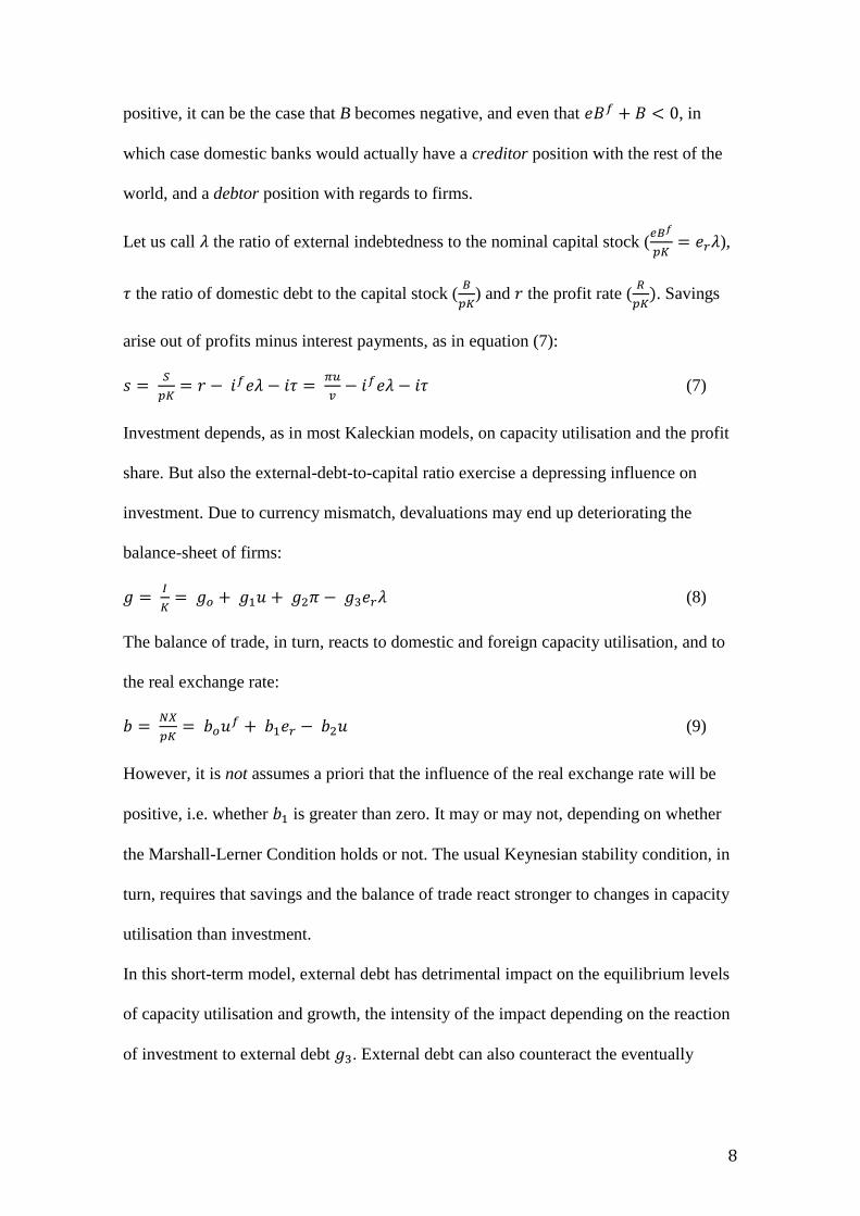
positive, it can be the case that B becomes negative, and even that 𝑒𝐵𝑓 + 𝐵 < 0, in

which case domestic banks would actually have a creditor position with the rest of the

world, and a debtor position with regards to firms.

Let us call 𝜆 the ratio of external indebtedness to the nominal capital stock (𝑒𝐵𝑓

𝑝𝐾= 𝑒𝑟𝜆),

𝜏 the ratio of domestic debt to the capital stock (𝐵

𝑝𝐾) and 𝑟 the profit rate (

𝑅

𝑝𝐾). Savings

arise out of profits minus interest payments, as in equation (7):

𝑠 = 𝑆

𝑝𝐾= 𝑟 − 𝑖𝑓𝑒𝜆 − 𝑖𝜏 =

𝜋𝑢

𝑣− 𝑖𝑓𝑒𝜆 − 𝑖𝜏 (7)

Investment depends, as in most Kaleckian models, on capacity utilisation and the profit

share. But also the external-debt-to-capital ratio exercise a depressing influence on

investment. Due to currency mismatch, devaluations may end up deteriorating the

balance-sheet of firms:

𝑔 = 𝐼

𝐾= 𝑔𝑜 + 𝑔1𝑢 + 𝑔2𝜋 − 𝑔3𝑒𝑟𝜆 (8)

The balance of trade, in turn, reacts to domestic and foreign capacity utilisation, and to

the real exchange rate:

𝑏 = 𝑁𝑋

𝑝𝐾= 𝑏𝑜𝑢

𝑓 + 𝑏1𝑒𝑟 − 𝑏2𝑢 (9)

However, it is not assumes a priori that the influence of the real exchange rate will be

positive, i.e. whether 𝑏1 is greater than zero. It may or may not, depending on whether

the Marshall-Lerner Condition holds or not. The usual Keynesian stability condition, in

turn, requires that savings and the balance of trade react stronger to changes in capacity

utilisation than investment.

In this short-term model, external debt has detrimental impact on the equilibrium levels

of capacity utilisation and growth, the intensity of the impact depending on the reaction

of investment to external debt 𝑔3. External debt can also counteract the eventually

9

positive impacts of real devaluations on capacity utilisation, if the Marshall-Lerner

Condition holds.

So far, this is a traditional short-run Kaleckian model. But in the medium-run, the

external-debt-to-capital ratio becomes and endogenous variable. This rises up the

question of how do firms fund their investment plans. They have three alternatives:

either through retained earnings, through domestic debt or through foreign debt. Debt

The latter is somewhat cheaper than the former, because of a liquidity premium usually

charged on domestic borrowing 𝜌0. Lenders are also concerned about booming debt,

and increase their lending rates accordingly, though the sensitivity of domestic and

external rates can be different:

𝑖 = 𝑖𝐵𝑓

+ 𝜌0 + 𝜌1𝑒𝑟𝜆 (10)

𝑖𝑓 = 𝑖𝐵𝑓

+ 𝜌1𝑓𝑒𝑟𝜆 (11)

There are a couple of issues to keep in mind. Debt dynamics is not only affected by

retained earnings and investment funding, but also with the repayment of principal and

interest. Second, in the model, there is a preferential order with regards to the sources to

fund investment and interest payments: retained earnings and external debt borrowing

take primacy with regards to domestic debt, which accommodates any difference

between required funds, retained earnings and external debt.:

𝐵 = 𝑝𝐼 − 𝑅 + 𝑒𝑖𝑓𝐵𝑓 + 𝑖𝐵 − 𝑒��𝑓 (12)

The reason behind is that external debt is usually cheaper than domestic borrowing, as

mentioned in equations 10-11.Third, external currency amounts to a proportion of total

investment, but that proportion is not constant. In fact, it changes with the difference in

the relative costs of both types of borrowing. In linear terms, we have:

𝑒��𝑓 = (𝜙0 + 𝜙1𝑒𝑟𝜆)𝑝𝐼 (13)

10

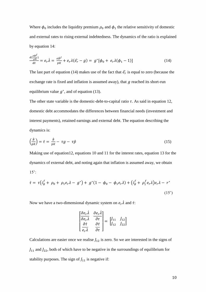
Where 𝜙0 includes the liquidity premium 𝜌0 and 𝜙1 the relative sensitivity of domestic

and external rates to rising external indebtedness. The dynamics of the ratio is explained

by equation 14:

𝑑(𝑒𝐵𝑓

𝑝𝐾)

𝑑𝑡= 𝑒𝑟�� =

𝑒��𝑓

𝑝𝐾+ 𝑒𝑟𝜆(𝑒�� − 𝑔) = 𝑔∗[𝜙0 + 𝑒𝑟𝜆(𝜙1 − 1)] (14)

The last part of equation (14) makes use of the fact that 𝑒�� is equal to zero (because the

exchange rate is fixed and inflation is assumed away), that 𝑔 reached its short-run

equilibrium value 𝑔∗, and of equation (13).

The other state variable is the domestic-debt-to-capital ratio 𝜏. As said in equation 12,

domestic debt accommodates the differences between financial needs (investment and

interest payments), retained earnings and external debt. The equation describing the

dynamics is:

(𝐵

𝑝𝐾

) = �� =

𝐵

𝑝𝐾

− 𝜏𝑔 − 𝜏�� (15)

Making use of equation12, equations 10 and 11 for the interest rates, equation 13 for the

dynamics of external debt, and noting again that inflation is assumed away, we obtain

15’:

�� = 𝜏(𝑖𝐵𝑓

+ 𝜌0 + 𝜌1𝑒𝑟𝜆 − 𝑔∗) + 𝑔∗(1 − 𝜙0 − 𝜙1𝑒𝑟𝜆) + (𝑖𝐵𝑓+ 𝜌1

𝑓𝑒𝑟𝜆)𝑒𝑟𝜆 − 𝑟∗

(15’)

Now we have a two-dimensional dynamic system on 𝑒𝑟�� and ��:

[ 𝜕𝑒𝑟��

𝜕𝑒𝑟𝜆

𝜕𝑒𝑟��

𝜕𝜏𝜕��

𝑒𝑟𝜆

𝜕��

𝜕𝜏 ]

= [𝐽11 𝐽12

𝐽12 𝐽22]

Calculations are easier once we realise 𝐽12 is zero. So we are interested in the signs of

𝐽11 and 𝐽22, both of which have to be negative in the surroundings of equilibrium for

stability purposes. The sign of 𝐽11 is negative if:

11

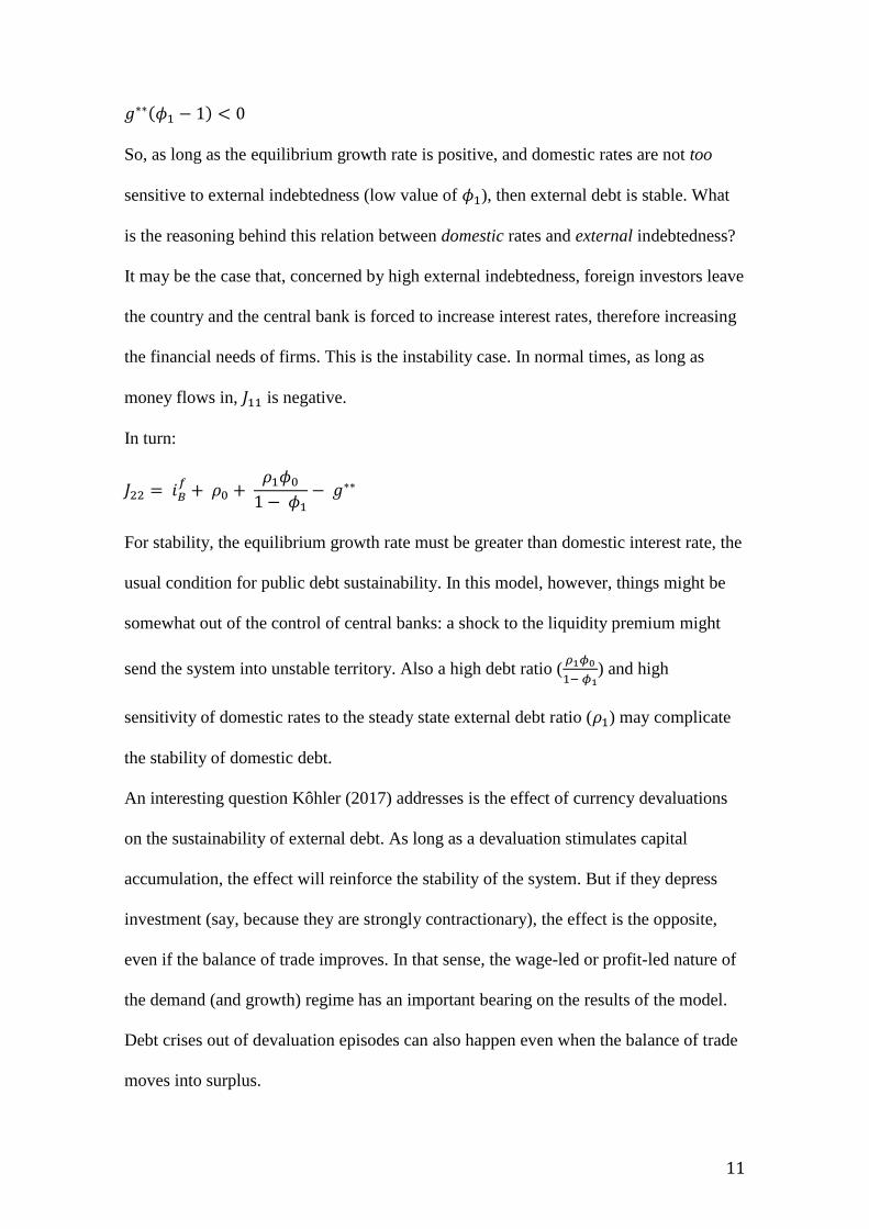
𝑔∗∗(𝜙1 − 1) < 0

So, as long as the equilibrium growth rate is positive, and domestic rates are not too

sensitive to external indebtedness (low value of 𝜙1), then external debt is stable. What

is the reasoning behind this relation between domestic rates and external indebtedness?

It may be the case that, concerned by high external indebtedness, foreign investors leave

the country and the central bank is forced to increase interest rates, therefore increasing

the financial needs of firms. This is the instability case. In normal times, as long as

money flows in, 𝐽11 is negative.

In turn:

𝐽22 = 𝑖𝐵𝑓

+ 𝜌0 + 𝜌1𝜙0

1 − 𝜙1− 𝑔∗∗

For stability, the equilibrium growth rate must be greater than domestic interest rate, the

usual condition for public debt sustainability. In this model, however, things might be

somewhat out of the control of central banks: a shock to the liquidity premium might

send the system into unstable territory. Also a high debt ratio (𝜌1𝜙0

1− 𝜙1) and high

sensitivity of domestic rates to the steady state external debt ratio (𝜌1) may complicate

the stability of domestic debt.

An interesting question Kôhler (2017) addresses is the effect of currency devaluations

on the sustainability of external debt. As long as a devaluation stimulates capital

accumulation, the effect will reinforce the stability of the system. But if they depress

investment (say, because they are strongly contractionary), the effect is the opposite,

even if the balance of trade improves. In that sense, the wage-led or profit-led nature of

the demand (and growth) regime has an important bearing on the results of the model.

Debt crises out of devaluation episodes can also happen even when the balance of trade

moves into surplus.

12

External flows and financial instability

The primordial role of growth in any debt sustainability analysis is in part related to the

importance of sales revenues and internal financing for “healthy” balance-sheet

positions. Kalecki (1971) underscored the relevance of internal finance as one of the

majour constraints on investment, while Minsky (1986) reflected on the tendency of

firms to rely increasingly on external financing (debt), which would lead to financial

fragility. Lavoie and Seccareccia (2001), however, doubt that this “Financial Instability

Hypothesis”, which could be valid at the firm level, still holds at a macroeconomic

level. They warn of a possible fallacy of composition. In the upward phase of the cycle,

as firms fund their increasing investment with borrowing, so will aggregate profits

increase; while in a downturn, though firms try to decrease their leverage, aggregate

profits will fall, making the whole effort futile. The argument is known as the “paradox

of debt”.

Guimaraes Coelho and Perez Caldentey (2018, GCPC from now on) develop an

interesting Kaleckian model that is flexible enough to accommodate both regimes,

while including the possibility of credit rationing due to increased liquidity preferences

of financiers. In an open economy setting that focuses on emerging economies, the

possibility of financing current account deficits depends on the availability of external

financing in foreign currency. The financial needs are measured, in GCPC model, by

the current account deficit, which is in turn influenced by the international liquidity, the

technological gap and income distribution, among other factors.

In order to review the open-economy model, it is convenient to do a quick summary of

the mechanisms it presents in a closed-economy setting. The open-economy version is

just an expansion of the former.

13

As it is usually the case in Kaleckian models, the key innovation lies in the investment

function. The one presented by GCPC is as follows:

𝑔𝑖 = 𝑎0 + 𝑎1ℎ + 𝑎2𝑢 + 𝑎3𝐼𝐹 + 𝑎4𝑓𝑏 (16)

Where ℎ is the profit share, 𝑢 is the capacity utilisation rate, 𝐼𝐹 captures the influence

of internal funds on investment, and 𝑓𝑏 captures the influence of external finance,

mostly banking finance in this closed-economy model. How do these last two variables

behave? What is the economic intuition behind them?

Internal funds capture the difference between gross profits and the cost of debt. The

major point that GCPC try to convey is that the sensitivity of gross profits and the cost

of debt to cyclical fluctuations may be different, depending on whether the financial

fragility hypothesis holds, or whether the paradox of debt holds. The equation is as

follows:

𝐼𝐹 = 𝛼1ℎ𝐾𝑢 − 𝛼2𝑖𝜃𝑢 (17)

In this setting, K represents the capital stock, i represents the interest rate and 𝜃

represents the leverage ratio. If 𝛼1ℎ𝐾 is greater than 𝛼2𝑖𝜃, then internal funds would

respond stronger than indebtedness to the business cycle (captured by u) and the

paradox of debt. If the other case holds, then internal funds decrease as the economy

grows, and we are in the financial instability hypothesis scenario. This is reflected on

the sign of the differential 𝜕𝐼𝐹

𝜕𝑢: if positive the paradox of debt holds, if negative the

financial instability hypothesis does. What about external finance? The following

equation captures its behaviour:

𝑓𝑏 = 𝑏1 − 𝑏2𝑑0𝜕𝐼𝐹

𝜕𝑢ℎ (18)

𝑏1 captures the liquidity preference of banks: the lower the preference, the higher the

value of 𝑏1. 𝑑0 is a dummy variable that captures the phase of the business cycle. If the

cycle is in the upward phase, 𝑑0 is worth 1, while if we are in the downward phase 𝑑0 is

14

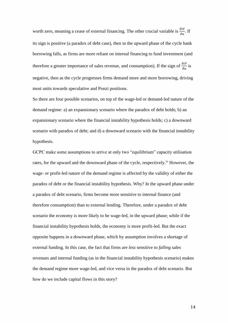
worth zero, meaning a cease of external financing. The other crucial variable is 𝜕𝐼𝐹

𝜕𝑢. If

its sign is positive (a paradox of debt case), then in the upward phase of the cycle bank

borrowing falls, as firms are more reliant on internal financing to fund investment (and

therefore a greater importance of sales revenue, and consumption). If the sign of 𝜕𝐼𝐹

𝜕𝑢 is

negative, then as the cycle progresses firms demand more and more borrowing, driving

most units towards speculative and Ponzi positions.

So there are four possible scenarios, on top of the wage-led or demand-led nature of the

demand regime: a) an expansionary scenario where the paradox of debt holds; b) an

expansionary scenario where the financial instability hypothesis holds; c) a downward

scenario with paradox of debt; and d) a downward scenario with the financial instability

hypothesis.

GCPC make some assumptions to arrive at only two “equilibrium” capacity utilisation

rates, for the upward and the downward phase of the cycle, respectively.iv However, the

wage- or profit-led nature of the demand regime is affected by the validity of either the

paradox of debt or the financial instability hypothesis. Why? In the upward phase under

a paradox of debt scenario, firms become more sensitive to internal finance (and

therefore consumption) than to external lending. Therefore, under a paradox of debt

scenario the economy is more likely to be wage-led, in the upward phase; while if the

financial instability hypothesis holds, the economy is more profit-led. But the exact

opposite happens in a downward phase, which by assumption involves a shortage of

external funding. In this case, the fact that firms are less sensitive to falling sales

revenues and internal funding (as in the financial instability hypothesis scenario) makes

the demand regime more wage-led, and vice versa in the paradox of debt scenario. But

how do we include capital flows in this story?

15

Some considerations are due at this point. First, GCPC take the current account balance

as the measure of external financing. Second, this finance is partly explained by the

liquidity conditions in international markets (again, through the 𝑏1 parameter in

equation 18). Third, the current account balance is also affected by the technological

gap and income distribution, though the latter is not determined a priori. If

redistribution benefits workers, their import demand will rise, but that of capitalist will

fall. GCPC assume that the latter effect will prevail, because of the capitalists’ high

demand for luxury goods.v

There are some equations therefore to include and some to modify. First, equation (18)

now has to include the determinants of the current account. GCPC use the ratio of

income elasticity of exports and imports, weighted by the state of capacity utilisation:

𝑓𝑏 = 𝑏1 − 𝑏2𝑑0𝜕𝐼𝐹

𝜕𝑢ℎ + 𝑏3

𝑒

𝜋𝑢 (18’)

Where e is the income elasticity of exports, and 𝜋 is the income elasticity of imports.

But as we said, GCPC postulate that the majour determinants of that ratio are the

technological gap and income distribution:

𝑒

𝜋= 𝑥1 + 𝑥2(1 − ℎ) + 𝑥3𝑇 (19)

Where 𝑇 captures the technological gap, and (1 − ℎ) represents the wage share. If we

replace (19) into (18’), we get (18’’):

𝑓𝑏 = 𝑏1 − 𝑏2𝑑0𝜕𝐼𝐹

𝜕𝑢ℎ + 𝑏3𝑥1𝑢 + 𝑏3𝑥2(1 − ℎ)𝑢 + 𝑏3𝑥3𝑇𝑢 (18’’)

And then substitute it into the investment equation (16).

The logic regarding the nature of the demand-regime in this open economy setting

remains virtually unchanged when compared to the closed economy framework. A

paradox of debt scenario, in the upward phase of the cycle, attaches greater influence to

internal funds over external lending, making the economy more wage-led, and the

opposite with the financial instability hypothesis. The eventual illiquidity in

16

international financial markets, in a downward phase, would make the financial

instability hypothesis case a more wage-led regime, because in this scenario firms

would be less sensitive to falling internal resources.

GCPC model is a step forward in the sense that it includes the effects of changes in

international liquidity conditions, and analyses different “financial regimes”. However,

it is still locked in the analysis of net capital flows. The next model to review breaks

with that cage.

Gross financial flows, income distribution and growth

Bortz, Michelena and Toledo (2018, BMT from now on) try to integrate the analysis of

three “stylised facts” of the last decades: a rise in global financial flows; an increase in

income inequality; and a slowdown of global growth compared to the post-war period.

The model recognizes the importance of gross financial flows (Ahmed & Zlate),

particularly through their influence on firms’ balance sheets. The main features of BMT

can be summarized in a few equations.

First, given that financial flows have a much higher order of magnitude than trade

flows, the model takes for granted that the nominal exchange rate moves with financial

flows, which are reflected in the (public and private) external debt d (normalized by the

capital stock):

�� = 𝜔�� (20)

Second, as for the drivers of financial flows, BMT distinguish endogenous and

exogenous factors, or “pull” and “push”, as they are called in the literature (Calvo et al

1996). Among the former, the state of aggregate demand is identify as a preponderant

variable (Nier, Sedik and Mondino 2014; Yildirim 2016), and BMT use capacity

utilisation as a proxy variable. Regarding “push” factors, which are the main

determinants of global financial flowsvi, BMT adopt a literature which identifies

17

heterogeneous agents in the foreign exchange market, usually called “chartists” and

“fundamentalists”.vii The former follow the short-term movement of the exchange rate,

which is usually influenced by interest-rate differentials. The latter follow some rule,

which in this model is determined by the difference between external indebtedness and

some assessed, conventional, tolerable indebtedness level, called 𝑑∗. This is represented

in equation (21):

�� = 𝑑𝑢𝑢 + 𝜇(𝑖 − 𝑖𝑓) + (1 − 𝜇)(𝑑 − 𝑑∗) (21)

The second major axis refers to income distribution. The model, just like La Marca’s,

captures wage-setting and price-setting behaviour by workers and firms, respectively.

They both have a wage-share target, which may not be mutually compatible. In

particular, the wage-share targeted by firms are influenced by their external borrowing

costs. Now, there is a thing with rising indebtedness and its impact on the exchange

rate. On the one hand, the volume of borrowing (and its cost in foreign currency) rises.

But on the other hand, the exchange rate appreciation makes it cheaper to borrow

abroad, and therefore the costs measured in domestic currency fall. Though BMT say

that they believe the first effect will prevail (the build-up of debt), the movement of the

wage-share targeted by firms takes into account both counteracting tendencies:

𝜓𝑓 = −𝑑1𝑑(𝛿 − 𝜔) (22)

Where 𝜓𝑓 is the wage-share targeted by firms; 𝑑1 is the share of private external debt

over total external debt; 𝛿 captures the impact of rising external debt, and 𝜔 captures

the effect of the exchange rate appreciation. As mentioned, BMT believe that, though in

the short-run it may be the case that 𝜔 is greater than 𝛿, in the medium to long-run the

experience tells us that the opposite is more likely to happen. Therefore, the “normal”

impact of rising external (private) debt on income distribution is to lower the wage

share.

18

The same counteracting forces influences productive investment. Rising debt volumes

may put pressure on firms’ balance sheet and restrict investment, but an appreciating

exchange rates makes external borrowing more attractive, on top of lowering the costs

of imported capital goods. On top of capacity utilisation and the profit share, the

investment function accounts precisely for those forces:

𝑔𝑓 = 𝑔0 + 𝑔𝑢𝑢 + 𝑔𝜋𝜋 + 𝑔𝑖𝑑1𝑑(𝛿 − 𝜔) (23)

These configurations of income distribution and effective demand can give rise to

alternative distributive, financial and demand regimes, which are summed up in Table 1

(which replicates Table 4 of BMT (2018)).

Table 1: List of alternative regimes

Derivative Regime Mathematical

Expression Meaning

𝜕��

𝜕𝑑

Exchange-rate

driven

𝜕��

𝜕𝑑> 0

Wage-share reacts positively to increments in foreign indebtedness.

Debt-service

driven

𝜕��

𝜕𝑑< 0

Wage-share reacts negatively to increments in foreign indebtedness.

𝜕��

𝜕𝑑

Debt-led 𝜕��

𝜕𝑑 > 0 Economic activity reacts positively to

increments in foreign indebtedness.

Debt-burdened 𝜕��

𝜕𝑑 < 0 Economic activity reacts negatively to

increments in foreign indebtedness.

𝜕��

𝜕𝜓

Wage-led 𝜕��

𝜕𝜓 > 0 Economic activity reacts positively to

increments in the wage share.

Profit-led 𝜕��

𝜕𝜓< 0 Economic activity reacts negatively to

increments in the wage share.

Source: Bortz, Michelena and Toledo (2018, p. 9).

The reaction of the wage share to movements in external debt can be called the

distribution regime; debt-led or debt-burdened are characteristics of the financial

regime, and wage-led or profit-led are alternative demand regimes. But which

combination of these regimes is stable? Table 2 (which replicates Table 5 of BMT) lists

all the possibilities, together with the equilibrium value of capacity utilisation in each of

the demand regimes.

19

Table 2: Stable Regime Combinations

Case 𝝏��

𝝏𝒅

𝝏��

𝝏𝒅

Equilibrium

capacity

utilization

NORMAL - - Wage-led: Higher

Profit-led: Lower

STRANGE + + Wage-led: Higher

Profit-led: Lower

CONCILIATING-

DEBT + -

Wage-led: Higher

Profit-led: Lower

Source: Bortz, Michelena and Toledo (2018, p. 9). What BMT call the “normal” regime is the combination of a debt-service driven

distribution regime with a debt-burdened financial regime. In this case, increments in

external debt lead to falling wage-share and falling aggregate demand, which is

exacerbated if the demand regime is wage-led, mainly due to rising debt service

payments and its pass-through to prices.

The “strange” case is the combination of an exchange-rate driven distribution regime (in

which rising debt causes strong exchange rate appreciations and rising wage-share) with

a debt-led financial regime (in which external borrowing is cheaper and stimulates

investment).

The “conciliating-debt” regime, finally, is a peculiar combination of an exchange-rate

driven distribution regime and a debt-burdened financial regime. In this case, the

exchange rate appreciation rises the wage share, but is not enough to stimulate

aggregate demand (mainly because of the deteriorating trade balance).

The model can be accommodated to include income policies. In an extension of the

model, BMT (2018) presents the feature of a Tax-based Income Policy (TIPs), in which

the government sets targets for the wage-share, and imposes them through marginally-

increasing tax rates on workers and firms.viii Therefore, the wage share is less sensitive

20

to exchange rate movements and to external debt fluctuations. The nature of the

distribution regime does not change, but its magnitude shrinks, both for the exchange-

rate driven or the debt-service driven. The economy is more likely to be wage-led,

however, in the case of progressive taxation.

One could also extend the model to incorporate some government-spending rule, as do

Bortz, Michelena and Toledo (2019). With an anti-cyclical government spending rule

the paradox of thrift is still maintained, but its impact is substantially mitigated. When

the rule takes into account fluctuating international financial conditions, government

spending becomes more pro-cyclical, leading to periods of “excessive” spending and

“excessive” austerity. In sum, the model is flexible enough to accommodate different

features and policies.

References

Ahmed, S. and Zlate, A. 2014. Capital flows to emerging market economies: a brave

new world, Journal of International Money and Finance, 48 (PB), 221-248.

Aizenman, J., Chinn, M. and Ito, H. 2016. Monetary policy spillovers and the trilemma

in the new normal: Periphery country sensitivity to core country conditions, Journal of

International Money and Finance, 68 (6), p. 298-330.

Akyüz, Y. 2014. Internationalization of finance and changing vulnerabilities in

emerging and developing economies, Discussion Paper No. 217, United Nations

Conference on Trade and Development, Geneva.

Amadeo, E. 1986. Notes on capacity utilization, distribution and accumulation,

Contributions to Political Economy, 5 (1), p. 83-94.

21

Bhaduri, A. and S. Marglin 1990. Unemployment and the real wage: The economic

basis for contesting political ideologies, Cambridge Journal of Economics 14(4): 375-

393.

Blecker, R. 1989. International competition, income distribution and economic growth,

Cambridge Journal of Economics 13(3): 395-412.

Blecker, R. 2002. “Distribution, demand and growth in Neo-Kaleckian macro models”,

in M. Setterfield (Ed.): The Economics of Demand-led Growth: Challenging the Supply-

Side Vision of the Long Run, Cheltenham, UK: Edward Elgar.

Blecker, R. 2011. Open economy models of growth and distribution, in E. Hein and E.

Stockhammer (eds.): A modern guide to Keynesian macroeconomics and economic

policies, Cheltenham, UK: Edward Elgar.

Bortz, P.G. 2016. Inequality, Growth and 'Hot Money', Cheltenham UK: Edward Elgar.

Bortz, P.G. and A. Kaltenbrunner. 2018. The international dimension of financialisation

in developing and emerging economies, Development and Change, 49 (2): 375-393

Bortz, P.G., Michelena, G. and Toledo, F. 2018. Foreign debt, conflicting claims and

income policies in a Kaleckian model of growth and distribution, Journal of

Globalization and Development, 9 (1), p. 1-22.

Bortz, P.G., Michelena, G. and Toledo, F. 2019. Non-conventional fiscal rules in a

Kaleckian model of growth and income distribution with external debt, in L.P. Rochon

and V. Monvoisin (eds): Finance, Growth and Inequality. Post-Keynesian Perspectives,

Cheltenham: Edward Elgar.

Bruno, V. and H.S. Shin. 2017. Global dollar credit and carry trades: A firm-level

analysis, Review of Financial Studies, 30(3): 703-749.

Calvo, G., Leiderman, R. and Reinhart, C. 1996. Inflows of Capital to Developing

Countries in the 1990s, Journal of Economic Perspectives, 10(2): 123-139.

22

Carrera, J., Rodriguez, E. and Sardi, M. 2016. The impact of income distribution on the

current account, Journal of Globalization and Development,, 7 (2), 1-20.

Cassetti, M. 2012. Macroeconomic outcomes of changing social bargains. The

feasibility of a wage-led open economy reconsidered, Metroeconomica, 63 (1), p. 64-

91.

Chui, M., Kuruc, E. and Turner, P. 2016: A new dimension to currency mismatches in

the emerging markets: non-financial companies, BIS Working Papers No. 550, Basilea.

Chutasripanich, N. and J. Yetman (2015). Foreign exchange intervention: Strategies and

effectiveness, BIS Working Papers No. 499.

Dutt, A. K. 1984. Stagnation, income distribution and monopoly power, Cambridge

Journal of Economics, 8 (1), p. 25-40.

Forbes, K. and F. Warnock 2012. Capital flow waves: Surges, stops, flight and

retrenchment, Journal of International Economics, 88(2): 235-251.

Frankel, J. and K. Froot 1990. Chartists, fundamentalists and trading in the foreign

exchange market, American Economic Review 80(2): 181-185

Goodwin, R. 1967. A growth cycle, in C.H. Feinstein (ed): Socialism, Capitalism and

Economic Growth, Cambridge: Cambridge University Press.

Guimaraes Coelho, D. and Perez Caldentey, E. 2018. Neo-Kaleckian models with

financial cycles: A center-periphery framework, PSL Quarterly Review, 71 (286), 309-

326.

Harvey, J. 1993. The institution of foreign exchange trading, Journal of Economic

Issues 27(3): 679-698.

Hein, E. 2014. Distribution and growth after Keynes. A Post Keynesian Guide.

Cheltenham, UK: Edward Elgar.

Kalecki, M. 1971. Selected Essays in the Dynamics of the Capitalist Economy,

Cambridge University Press, Cambridge.

23

Köhler, K. 2017. Currency devaluations, aggregate demand and debt dynamics in an

economy with foreign currency liabilities, Journal of Post Keynesian Economics 40(4):

487-511.

La Marca, M. 2005. Foreign debt, growth and distribution in an investment-constrained

system, in N. Salvadori and R. Balducci (eds.): Innovation, Unemployment and Policy

in the Theories of Growth and Distribution, Edward Elgar, Cheltenham.

La Marca, M. 2010. Real exchange rate, distribution and macro fluctuations in export-

oriented economies, Metroeconomica 61(1): 124-151.

Lavoie, M. 2014. Post-Keynesian Economics-New Foundations. Cheltenham, UK:

Edward Elgar.

Lavoie, M. and G. Daigle 2011. “A behavioral finance model of exchange rate

expectations within a stock-flow consistent framework”, Metroeconomica 62(3): 434-

458.

Lavoie, M. and Seccareccia, M. 2001. Minsky’s financial fragility hypothesis: a missing

macroeconomic link?, in R. Bellofiore and P. Ferri (eds.): Financial Fragility and

Investment in the Capitalist Economy: The Economic Legacy of Hyman Minsky, Volume

II, Cheltenham: Edward Elgar.

Minsky, H. 1986. Stabilizing an Unstable Economy, New York: McGraw Hill.

Nier, E., T. Sedik and T. Mondino 2014. Gross private capital flows to emerging

markets: Can the global financial cycle be tamed?, IMF Working Paper No.

14/29.

Ribeiro, R., McCombie, J.S.L and Lima, G.T. 2017. Some unpleasant currency-

devaluation arithmetic in a post Keynesian macromodel, Journal of Post Keynesian

Economics, 40 (2), p. 145-167.

Rowthorn, R. 1981. Demand, real wages and economic growth, Thames Papers in

Political Economy, Autumn, p. 1-39

24

Von Arnim, R.(2011): Wage policy in an open-economy Kalecki-Kaldor model: a

simulation study,Metroeconomica, Vol. 62 (2), pp. 235-264.

Yildirim, Z. 2016. Global financial conditions and asset markets: Evidence from fragile

emerging economies, Economic Modelling 57 (September 2016): 208-220.

i A revision of Kaleckian models of growth and distribution can be found in Blecker

2002), Hein (2014) and Bortz (2016), among others. Lavoie (2014, chapter 6) reviews

several topics addressed through extended versions of Kaleckian models. ii A revision of this literature can be found in Köhler (2017, p. 489-490). See as well

Lavoie (2014, pp. 532-540). iii See Lavoie (2014, chapter 3) for a detailed exposition and related references. iv They assume that, in an upward scenario with paradox of debt, the increase in 𝑏1

will overcome the negative effect on external finance of rising internal funds 𝜕𝐼𝐹

𝜕𝑢, as

can be seen in equation 18. v Carrera et al (2016) find opposing results for a sample of 60 countries, including 35 emerging economies. One could only speculate, but the diffusion of consumption patterns through new communication outlets in the last decades may have homogenized consumption patterns across different social classes. vi Among others, see Forbes and Warnock (2012), Ahmed and Zlat (2014), Aizenman et al (2016) and Bruno and Shin (2017). vii Among others, see Frankel and Froot (1990), Harvey (1993), Lavoie and Daigle (2011), and Chutasripanich and Yetman (2015). viii A similar logic would apply if the government opts for a subsidy policy instead of a tax policy.