discrimination among populations of sockeye salmon fry with

Transactions of the American Fisheries Society 126:559-578. 1997American Fisheries Society 1997

Discrimination among Populations of Sockeye Salmon Fry withFourier Analysis of Otolith Banding Patterns

Formed during IncubationJAMES E. FINN, CARL V. BURGER,' AND LESLIE HOLLAND-BARTELS

Alaska Science Center, U.S. Geological Survey, Biological Resources Division1011 East Tudor Road, Anchorage, Alaska 99503, USA

Abstract.—We used otolith banding patterns formed during incubation to discriminate amonghatchery- and wild-incubated fry of sockeye salmon Oncorhynchus nerka from Tustumena Lake,Alaska. Fourier analysis of ololith luminance profiles was used to describe banding patterns; theamplitudes of individual Fourier harmonics were discriminant variables. Correct classification ofotoliths to either hatchery or wild origin was 83.1% (cross-validation) and 72.7% (test data) withthe use of quadratic discriminant function analysis on 10 Fourier amplitudes. Overall classificationrates among the six test groups (one hatchery and five wild groups) were 46.5% (cross-validation)and 39.3% (test data) with the use of linear discriminant function analysis on 16 Fourier amplitudes.Although classification rates for wild-incubated fry from any one site never exceeded 67% (cross-validation) or 60% (test data), location-specific information was evident for all groups becausethe probability of classifying an individual to its true incubation location was significantly greaterthan chance. Results indicate phenotypic differences in otolith microstructure among incubationsites separated by less than 10 km. Analysis of otolith luminance profiles is a potentially usefultechnique for discriminating among and between various populations of hatchery and wild fish.

The stock concept in management of salmonidpopulations has been in use since the latter part ofthe 19th century. Because the life histories of Pa-cific salmon Oncorhynchus spp. include a high de-gree of fidelity to discrete spawning areas (Ricker1972; Blair and Quinn 1991), populations may belocally adapted to their specific spawning, incu-bation, and rearing environments (Taylor 1991).Genetically discrete stocks of Pacific salmonspawning within the same drainage occur in pinkO. gorbuscha, sockeye O. nerka, chinook O. tshaw-ytscha, and chum salmon O. keta (Wilmot and Bur-ger 1985; Adams et al. 1994; Wilmot et al. 1994;Smoker et al., in press). Also, when genetic evi-dence is unavailable or inconclusive, there is eco-logical and behavioral evidence to suggest that lo-cally adapted stocks may co exist within relativelysmall (<10 km) ranges (Holland-Bartels et al.1994). Individuals from several potentially dis-crete spawning populations often rear in a commonenvironment throughout much of their life. Forexample, early- and late-run sockeye salmon mayspawn in different environments (tributary versuslake shorelines); however, their young rear in acommon lake environment (Burgner 1991). There-fore, studies of population dynamics during the

1 Present address: U.S. Fish and Wildlife Service, Ab-ernathy Salmon Culture Technology Center, 1440 Ab-ernathy Road, Longview, Washington 98632, USA.

freshwater phase require some means of discrim-inating individual populations.

Fishery biologists have used a host of tech-niques to separate fish populations. Artificialmarking includes fin clipping, branding, and cod-ed-wire-tagging (Jewell and Hager 1972; Nielsen1992); chemical marking of calcified structures(Mulligan et al. 1987; Yamada and Mulligan 1990;Hendricks et al. 1991); and genetic markers (Ih-seenetal. 1981; Lane et al. 1990; Seebet al. 1990;Gharrett et al., in press). To circumvent the as-sumption that marked and unmarked individualsbehave similarly, naturally occurring patterns inscale patterns have been used to separate Pacificsalmon (Rowland 1969; Cook and Lord 1977;Cook 1982; Cross et al. 1987). However, this meth-od is limited when populations are of close geo-graphic origin or when potential discriminatingfactors are fixed before scale formation, as mightbe the case for fry incubated in tributaries, lakeshorelines, or hatcheries.

Otoliths provide a tool for study of the originof fish populations through their elemental com-position (Rieman et al. 1994) and microstructure(Pannella 1971). Although increment depositionmay be tied to an endocrine-driven, endogenouscircadian rhythm (Campana and Neilson 1985),factors such as water temperature, photoperiod,and feeding frequency may modify or mask theeffects of diurnal rhythms (Marshall and Parker1982; Neilson and Geen 1984). Stress and life his-

559

560 FINN ET AL.

tory events such as hatching, first feeding, andmigration from freshwater to salt water, can berecorded in otoliths (Marshall and Parker 1982;Volk et al. 1984; Neilson et al. 1985a; Brothers1990; Paragamian et al. 1992; Hendricks et al.1994). However, for them to be valuable for stockidentification of sockeye salmon and other Pacificsalmonids, otoliths must form sufficiently earlyand be capable of recording incubation environ-ments. Such evidence does exist for salmonid oto-liths (Neilson et al. 1985b; Brothers 1990; Volk etal. 1990), which form by the time embryos reachthe eyed egg stage. In addition, temperature alonehas been shown to strongly influence otolith band-ing during incubation (Volk et al. 1990).

Naturally occurring differences in otolith struc-ture formed during incubation and larval stageshave been reported for a wide range of speciessuch as between summer and winter steelhead(anadromous form of rainbow trout O. mykiss)(McKern et al. 1974) and between steelhead andresident rainbow trout (Rybock et al. 1975). How-ever, Neilson et al. (1985b) found within-groupvariability in nucleus size that limited their abilityto use this measure to separate steelhead and res-ident rainbow trout. This disparity occurred de-spite the fact that young were incubated under con-trolled conditions, in which group variabilityshould have been minimized. Ambiguity in defin-ing the border of the nucleus, in defining checkmarks, and in establishing reference points andtransects introduce error into increment counts anddimension measures (Wilson and Larkin 1982;Gun-ens et al. 1988; Neilson 1992). We propose anew method that permits examination of variationand components of the overall banding pattern andreduces the subjectivity introduced by artificial def-initions of reference points, transects, and incre-ment boundaries.

Fourier analysis allows for the decompositionof complex periodic functions into discrete sub-components. Fourier shape analysis has been usedto discriminate fish stocks by scale (Jarvis et al.1978; Riley and Carline 1982) and otolith shape(Birdetal. 1986;Castonguay etal. 1991;Campanaand Casselman 1993; Friedland and Reddin 1994).However, otolith shape at the time of collectionilluminates little about differences that occurredduring incubation. In contrast, the banding patternlaid down during incubation remains unchangedby subsequent life history events (Campana andNeilson 1985). It is this banding pattern of darkand light intensities (luminance values) across anotolith transect (luminance profile) that can be rep-

resented by a complex periodic function describedwith Fourier analysis. Therefore, Fourier analysisof luminance profiles may permit discriminationamong fish that experience different incubation en-vironments.

The Alaska Department of Fish and Game(ADFG) began a program in 1976 that releasedhatchery-incubated emergent sockeye salmon fry(fed for several weeks) into Alaska's TustumenaLake. Eggs obtained from adults returning tospawn each year in two of the lake's tributaries(Bear and Glacier Flats creeks), were incubated atnearby Crooked Creek Hatchery (Figure 1) andreleased directly into the lake (Kyle 1992). Be-cause fry that incubated at the hatchery and withinthe lake's drainage experienced different thermalregimes (Figure 2), we hypothesized that these dif-ferences would produce varying otolith bandingpatterns and hence, provide a way to discriminatepopulations. This could help in future studies ofthe competitive interactions between hatchery-and wild-incubated young and in discriminatingwild fry originating from the various spawningareas in the drainage.

The purpose of this study was to determine thefeasibility of using otolith microstructure, as de-scribed by Fourier analysis, to discriminate amongvarious sockeye salmon populations rearing withina glacially turbid lake system in Alaska. Specificobjectives were (1) to develop standardized tech-niques for the measurement of otolith microstruc-ture characteristics, (2) to test for differences inthe characteristics among sockeye salmon fry orig-inating from various locations in the TustumenaLake drainage, and (3) to test discriminant modelsbased on banding characteristics.

Study SiteTXistumena Lake is within the Kasilof River wa-

tershed, south-central Alaska, and is includedwithin the Kenai National Wildlife Refuge (Figure1). The 40-km-long, 8-km-wide lake is the largest(about 295 km2) on the Kenai Peninsula and hasmean and maximum depths of 124 m and 320 m.The lake is glacially turbid (about 50 nephelo-metric turbidity units; light penetration, <2 m) andoligotrophic (total phosphorus averages 3.7 (ig/Lduring May-October) due to meltwater from Tus-tumena Glacier (Kyle 1992).

Sockeye and chinook salmon are the most com-mercially and recreationally important Pacificsalmon species that occur in the system. The sys-tem supplies up to 20% (2 million fish) of CookInlet's total annual sockeye salmon harvest; esti-

OTOLITH DISCRIMINATION OF SOCKEYE SALMON 561

Sockeye Salmon FrySampling Sites

FIGURE 1.—Sampling sites used in analysis of otolith banding patterns of sockeye salmon fry from TustumenaLake, Alaska.

0.015-Aug 7-Oct 29-Nov 21-Jan 15-Mar 7-May

Date7-Oct 29-Nov 21-Jan 15-Mar 7-May

FIGURE 2.—Daily median water temperatures (°C) for Crooked Creek Hatchery, and Bear, Glacier Flats, andNikolai creeks, Tustumena Lake drainage, Alaska, for various brood years (e.g.. 1989: fry spawned during 1989emerged and migrated into the Lake during spring 1990). Hatchery temperatures not monitored from mid-Octoberto early April.

562 FINN ET AL.

mated exploitation rates of the lake's sockeyesalmon in the commercial fishery range from 50%to 85% (Kyle 1992). About one-third of all sock-eye salmon in the system spawn along the lake-shore (Burger et al. 1995); 96% of the remainingspawners are distributed in four tributaries (Bear,Glacier Flats, Moose, and Nikolai creeks; Kyle1992). Annual hatchery releases have ranged from400,000 to 17,050,000 fry, and the annual stockinglevel has been 6,000,000 fry since 1988. Hatchery-incubated fish average about 26% (1981-1990) ofthe estimated smolt outmigration (Kyle 1992).

MethodsSample collection and selection.—Six groups of

sockeye salmon fry were collected and preservedin ethyl alcohol (>80%; Butler 1992) during 1992:hatchery fish, the shoreline spawning group at Gla-cier Springs and fish from Bear, Glacier Flats,Moose, and Nikolai creeks (Figure 1). Fry fromtributaries were collected as they migrated fromincubation areas. At each of Bear, Glacier Flats,and Nikolai creeks, we preserved a sample of fry(N = 100) every 7 d from 22 April to 2 June andtook an additional sample during peak migration.Moose Creek was sampled three times during thesame time period. Collection of fry for the shore-line sample was more problematic. We beachseined regularly where Burger et al. (1995) haddocumented sockeye salmon spawning activity butcollected no more than 50 fry. However, on 2 Juneseveral hundred fry were dipnetted as they mi-grated from clear water springs (Glacier Springs)along the lake shore (Figure 1). These fish con-stitute our shoreline-incubated sample. Hatcheryfry (N > 100) were dipnetted from hatchery race-ways on each of three sampling dates (3, 14, and15 June). In addition to the fry preserved in al-cohol, samples from all locations were preservedin 10% formalin for length and weight measure-ments and for examination of stomach contents.

When fry from multiple dates were available,subsamples were taken by selecting the peak mi-gration date and then randomly selecting one totwo dates before and after the peak date. We se-lected fry from all three of the hatchery samplingdates. From each of the dates used, 50 fry wererandomly selected, except that the Glacier Springssample included 100 fry randomly sampled on asingle date.

Otolith preparation.—Our morphological ter-minology follows Pannella (1980). We used thelargest of the three pairs of otoliths, the sagittae.(Hereafter, our use of the word otolith refers to the

sagittae.) Fry were measured (nearest 0.1 mm, forklength), and otoliths were removed and mountedproximal (sulcus) side down on microscope slideswith a thermoplastic glue (Secor et al. 1992) andpolished to the primordial zone on the sagittalplane with a lapidary wheel and 1.0-u,m and 0.05-jjim alumina paste. The polishing process was re-peated on the distal side of each otolith.

Feature extraction.—We examined otolith band-ing features with a transmitted-light microscope,video camera, microcomputer-based digital imageanalysis system, and Optimas (Bioscan, Inc., Se-attle) image analysis software (Finn 1995). Themicroscope illumination level was held constantfor all samples. This process provided a digitizedimage with luminance intensity measured on agrey scale of black (0) to white (255).

All measurements were taken along transects inthe posterior dorsal quadrant of each sagitta (Fig-ure 3), the zone with the greatest growth and bestincrement definition (Pannella 1980; Marshall andParker 1982; Wilson and Larkin 1982; Campanaand Neilson 1985). To allow application of ourtechnique to older fish, we developed a protocolfor the placement and length of measurement tran-sects that was not based on reference points (e.g.,rostrum, postrostum) that can change with fish orotolith growth. In addition, our technique placedtransects so that they would include the majorityof the otolith formed during incubation, but wouldnot to include areas formed after fry migrate intocommon lake-rearing environments. We used arandom sample of 67 wild-incubated fry otolithsfrom the four tributary groups to define this zone.Otoliths were measured from the most posteriorprimordia to the otolith edge along three transectsat 40, 60, and 80° angles off a reference line run-ning from the rostrum through the most posteriorprimordia (N = 201; mean = 230.0 fxm; range =169.5-309.0 |xm; SD = 32.6 |xm). Based on thesedata, we selected a distance of 160 jjim for the endpoint of transects starting at a central primordia,a distance including 55-96% of the zone formedduring incubation (0.95 probability) with a prob-ability of less than 0.016 of including otolith band-ing formed after migration into the lake.

For examination of banding patterns, we se-lected a portion of the posterior quadrat that in-cluded both a distinct primordium and clear band-ing, and we subjectively eliminated areas withcracks, scratches, and excessive polishing. Tran-sects were then placed perpendicular to the otolithbands. However, before collecting data from tran-sects, the contrast between light and dark bands

OT01.1TH DISCRIMINATION OF SOCKEYF. SALMON 563

(A)Posterior Dorsal

QuadrantPrimordia

V,

Rostrum

FIGURE 3.—(A'l Distal perspective of soekeye salmon fry otolith with major features indicated. All luminanceprofiles were measured in the stippled area (posterior dorsal quadrant). (B) Otolilh image and inserted line graphsshow three 150-p.m transects, banding pattern, and luminance profiles (1) prior to application of convolution edgedetection filter and (2) after filtering.

was enhanced by applying a 3 X 3 edge detectionconvolution mask (Figure 3; Gonzalez and Wintz1987). Then, the primordium was selected as areference for transect positions. To avoid includingthe primordium, we began the center transect 10|xm above the start point, resulting in a 150-p,msection analyzed for luminance patterns. The othertwo transects were positioned 5 jxm to the left andright of the center transect (Figure 3). Because thealgorithm we used for our analyses (described be-low) required a data series whose N was of an evenpower (e.g., 64, 128, 256, 512), we selected a dataseries of 256 measurements along our 150-u.mtransect, resulting in luminance values measuredevery 0.586 jxm along each of the three transects.Each luminance value was averaged over a widthof five pixels (about 3 juim) according to proceduresdescribed by Finn (1995). Thus, each otolith hadthree 150-jxm, 256-value luminance transects ex-tracted to spreadsheet data files. In order to inte-grate the luminance data from the three transects,the luminance values (L) were averaged over thethree transects (/ = 1-3) at each of the; = 1 ...256 intervals as follows:

}Lf = % Lu/3.

i-\

This resulted in one average luminance profile per

otolith. Average luminance values were then stan-dardized to have a mean = 0 and standard devi-ation = 1 by subtracting the transect mean lumi-nance and dividing by the transect standard de-viation.

Fourier transformation.—The average lumi-nance profiles were transformed into a Fourier se-ries with a fast Fourier transformation (FFT) al-gorithm (Gonzalez and Wintz 1987; Microsoft Ex-cel 4.0, Microsoft Inc., Redmond, Washington),which decomposed the series into component co-sine functions. Cosines are additive such that theluminance value at any given point can be de-scribed as

(1)

Lx - luminance value at point / along the tran-sect;

AO = amplitude of the Oth harmonic (amplitudeassociated with mean luminance);

AJ = amplitude of the /th harmonic;9/ = polar angle of the /th harmonic; and

4>/ = phase angle of the /th harmonic.

Equation (1) was adapted from Fourier shapeanalysis (Jarvis et al. 1978) in which the shape is

564 FINN ET AL.

defined by radii from a centroid by using polarangle coordinates. It can easily describe the shapeof a luminance profile if the profile is consideredto be an unrolled-shape perimeter and the coor-dinates along the Jt-axis are considered distancesalong a transect, rather than degrees around a polarplot (Jarvis et al. 1978). The luminance profile willbe exactly described by a summation of N = 256harmonics at each point of the transect. However,there were only N/2 - 256/2 = 128 unique har-monics. The portion of the pattern accounted forby individual or subset harmonics was determinedby setting all other harmonics to zero and per-forming an inverse FFT.

In practice, software algorithms produced acomplex number for each point along the lumi-nance profile. This complex number was of theform

z = x + yit

where jc = a real number; and yi = an imaginarynumber. Then the amplitude for a given harmonicis defined as

At = \z\ = V*2 + y2.

The variance of each harmonic is given by

Vk = Al/2.

As these variances are additive (Jarvis et al. 1978),the proportion of the total variation accounted forby individual and subsets of harmonics is calcu-lated as

Nl2ck = Ak

The individual amplitudes were used as vari-ables in statistical analyses. Although the phaseangle (4>) contains shape information, 4> is distrib-uted in a circular manner and is often bimodal(Campana and Casselman 1993). Therefore, thereare no means to transform <1> to approximate nor-mality.

Statistical analysis. — Although univariate nor-mality does not insure multivariate normality, testsfor multivariate normality are limited (Johnsonand Wichern 1988). Therefore to evaluate depar-tures from univariate normality, Lilliefor's test wasapplied to individual amplitudes (Daniel 1990;SYSTAT 1992). The distributions of the untrans-formed amplitude variables were all nonnormal(Lilliefor's test; Dmax > 0.059; P < 0.001). Trans-formations were selected from the family knownas Box-Cox power transformations (Sokal and

Rohlf 1981; Johnson and Wichern 1988). The gen-eral form of the transformation is

X' = (X* - 1)/X for X * 0;

X' = \oge(X) for X = 0.

The "best" value of X is that value which maxi-mizes the log-likelihood function, L (Sokal andRohlf 1981). Lambda was evaluated separately foreach of the 128 amplitudes over a range of0.10-1.00 in increments of 0.05. After Box-Coxpower transformation, only 6 of the 128 ampli-tudes were significantly nonnormal (P < 0.05).Therefore, all analyses were performed with theabove transformation. In contrast, other transfor-mations were less effective; the square root trans-formation left 43% of the amplitudes significantlynonnormal, and the natural log transformation,99%.

Data sets were developed to (1) test for differ-ences between left and right otoliths, (2) test fordifferences between readers, (3) estimate discrim-inant functions (learning data), and (4) test dis-criminant functions (test data). Luminance profileswere recorded on 1,203 otoliths. Of these, 427pairs (left and right from the same fish) were avail-able for testing differences between left and rightotolith luminance profiles. To test for consistencybetween observers, a random sample of 50 otolithswas independently remeasured by a second ob-server.

Randomized block analysis of variance (ANO-VA) on individual amplitudes indicated little dif-ference between left and right otoliths; only 13(10.2%) of the 128 amplitudes were significantlydifferent (P < 0.05) between left and right otoliths.Therefore, we felt justified in the random use ofeither left or right otoliths in learning and test datasets. When paired otoliths were present, left orright otolith values were randomly deleted. Thisprocedure resulted in a data set of 776 luminanceprofiles that was subdivided into learning and testdata sets. For the test data set, a random sampleof 25 luminance profiles was taken from each ofthe six incubation groups (total = 150). The re-maining 626 observations made up the learningdata set.

We attempted to classify individuals into m =2 groups (hatchery versus wild) and m = 6 groups(hatchery, Bear Creek, Glacier Flats Creek, Gla-cier Springs, Moose Creek, and Nikolai Creek).Linear (LDF) and quadratic (QDF) discriminantfunctions were used to develop classification ruleswith the learning data set (SAS Institute 1989b;


Huberty 1994). The LDF provide optimal discrim-ination rules under the assumptions of multivariatenormality and equality among group covariancematrices (homoscedasticity). The QDF classifica-tion rules assume multivariate normality; however,the assumption of homoscedasticity is relaxed(Huberty 1994). The assumption of homoscedas-ticity was tested with Bartlett's log-likelihood ratio(SAS Institute 1989a; McLachlan 1992). Althoughthe form of the data provided guidance for selec-tion of statistical techniques (McLachlan 1992;Huberty 1994), the success (classification rate) ofthe rule in assigning individuals to the correctgroup is the most important criteria for populationseparation. Classification rates were estimatedwith the learning data with cross-validation (alsoknown as the Lachenbruch's "holdout" or "Icavc-one-out" technique; Johnson and Wichern 1988;McLachlan 1992) and by applying discriminantrules to the test data.

A problem with Fourier analysis of luminancevalues is the large number of variables (128) avail-able for the discriminant model. A general rule isto restrict the number of discriminant variables top < W//3, where /V/ = the sample size of the small-est group (Williams and Titus 1988). As a startingpoint, we used two methods to select initial subsetsof variables. The first method, forward-backwardstepwise LDF (SAS Institute 1989b) was used toselect variable subsets for LDF model develop-ment. The second method (ANOVA) provided ini-tial variable subsets for QDF model development.Univariate ANOVA (SAS Institute 1989a) wasdone on individual amplitudes to test for signifi-cant differences among groups. Amplitudes thatwere highly significantly different (P ̂ 0.01) wereincluded in the initial QDF models.

Starting with reduced sets of p amplitudes, re-finement was done by running PROC DISCRIM(SAS Institute 1989a) on all combinations of p -1 amplitude sets and examining the estimated clas-sification (cross-validation) rates. This processwas continued until the p = 1 amplitude modelwas reached. We used SAS programs to calculatethe total cross-validation classification rate as theaverage of the rates realized by the individualgroups (SAS Institute 1989a). After initial modelselection, total classification rates were calculatedas the total (all groups combined) number of oto-liths correctly classified divided by the total sam-ple size. The three models that resulted in the high-est classification rates were used for classificationof the test data set. Pairwise comparisons of clas-sification rates were done with McNemar's test for

related samples (Daniel 1990; Huberty 1994). Theoverall experimentwise error rate was set at a =0.1 (Daniel 1990). Then the individual comparisonsignificance level was a' = 0.1 /[/:(£-!)], where kis the total number of pairwise comparisons. Todetermine whether the classification rates weregreater than could be expected by chance, the ob-served number (OK) classified to the correct originwas compared to the expected number (eK). Theexpected number, calculated under assumptions ofequal and independent probabilities of classifica-tion, was eK = l/m-n^ where nK = the number ofindividuals whose true origin was location g, andm = the number of possible origins. The test sta-tistic was

Under the null hypothesis (//Q), OK - eg = 0, z hasa standard normal distribution (Huberty 1994).Chi-squarc tests of independence were used to de-termine whether the proportions of correctly clas-sified otoliths were significantly different amonglocations and sample dates (Daniel 1990).

ResultsOtolith Samples

We extracted and polished otoliths from 776sockeye salmon fry (Table 1). The difference be-tween the actual sample size and the target samplesize (100 for Glacier Springs and 50 for all othersite and date combinations) reflects the loss of oto-liths during extraction, breakage, and excessivepolishing. The loss of otoliths ranged from 4% to32% (Table 1).

Hatchery fry (mean = 29.3 mm) were signifi-cantly larger (/ = 10.78, P < 0.001) than wild fry(mean = 27.6 mm). Mean lengths were signifi-cantly different among the six groups (ANOVA;F = 48.12, df = 5, N = 769, P < 0.001). PairwiseTukey comparisons indicated that the hatchery andGlacier Springs fry were similar and larger thanfry from other locations (Figure 4). This differencewas expected as hatchery fry were all sampled inJune and most had been fed for several weeks. TheGlacier Springs fry were also sampled later thanmost other wild fry. Pairwise comparisons amongthe other wild fry groups indicated that MooseCreek fry were significantly smaller (P ^ 0.001;Figure 4) than other wild groups. Little feeding,as indexed by the percentage of stomachs con-taining food items, was observed in fry from Bear(0.2%), Moose (0.0%), and Nikolai (0.7%) creeks

566 FINN ET AL.

TABLE 1.—Sample location, date and fork lengths (mm)of preserved Tustumena Lake. Alaska, sockeye salmon fryused in otolith pattern analysis.

Fork length

Location and dale Mean (range) SE

Crooked Creek Hatchery3 Jun

14 Jun15 Jun

Bear Creek20 Apr18 May21 May

2 JunGlacier Flats Creek

22 Apr27 Apr4 May

29 MayGlacier Springs

2 Jun

28.3 (26.1 - 31.7)30.1 (27.4-34.5)29.3 (25.7 - 33.8)

27.8 (24.8 - 29.3)27.4 (25.2 - 29.2)27.3 (25.0 - 29.8)27.3 (24.5 - 28.9)

26.9 (24.7 - 31.6)27.1 (25.8-29.1)27.3 (25.4 - 32.9)28.9 (24.7 - 33.7)

1.131.601.73

404748

0.93 470.89 480.98 381.01 49

1.48 340.82 341.55 492.47 47

28.8(25.3- 31.4) 1.2785Moose Creek

29 Apr22 May

Nikolai Creek27 Apr4 May

25 May

26.5(22.1 -29.7)26.9 (23.5 - 28.9)

27.4(24.4-29.1)28.1 (26.4- 29.7)27.3 (25.0 - 29.4)

1.871.12

0.970.761.05

3740

444940

(J. Finn, unpublished data). On the other hand,33.4% of the Glacier Flats Creek and 86.0% of theGlacier Springs fry stomachs contained food (pre-dominantly chironomid larvae, pupae, and adults).

Amplitudes were not significantly affected byobserver. Significant differences between observermeasurements were found for only 3 (2.4%) of the128 amplitude comparisons (randomized blockANOVA; P < 0.05) between the two observers.Although not a rigorous test (i.e., the results fromonly two observers were compared), the methodused for feature extraction was repeatable and canbe performed with limited instruction.

Hatchery versus Wild Sockeye SalmonComparisons of amplitude between hatchery

and wild sockeye salmon resulted in significantdifferences (ANOVA; P < 0.01) for 30 (23.4%)amplitudes. Although amplitudes within the hatch-ery data set were neither consistently higher norlower than amplitudes in the wild samples, thelargest differences were seen in amplitudes 20-28(Figure 5). Stepwise discriminant analysis initiallyselected 29 amplitudes and of those, 18 (62.1%)were significantly different in the previous ANO-VA. These subsets of amplitudes (30 from ANO-VA and 29 from stepwise discrimination) formed

422 2*'Fork Length (mm)

FIGURE 4.—Percent frequency distributions of forklengths of preserved sockeye salmon fry used in otolithpattern analysis, Tustumena Lake, Alaska. 1992. Inserthistograms are distributions by sample date for each lo-cation.

the starting points for looping procedures to selectmore parsimonious subsets of amplitudes.

Linear discriminant analysis.—During the loop-ing process on the 29 amplitudes selected by step-wise discriminant analysis, the total average cross-validation classification rates ranged from 0.646to 0.861 for models with/? = 29 through 1 (Figure6A). The LDF models that resulted in the threehighest total average classification rates included20, 24, and 26 amplitudes (Table 2). The LDFclassification rates based on cross-validation were84% or better for both hatchery and wild otoliths.However, when LDF was used to classify the testdata, the classification rates were less than 75.0%(Table 2). The best classification of test data was60.0% (hatchery) and 77.6% (wild) with the24-amplitude model. None of the pairwise com-parisons between the 20-, 24-, and 26-amplitudemodels were significant (McNemar's test; \z\ ^0.080, P > 0.02) for both cross-validation and testdata classification rates. The assumption of equal-ity of covariances was rejected (Bartlett's log-like-lihood ratio; P < 0.001) for all three LDF models.

Quadratic discriminant analysis.—Starting with


9.5 •

8.5 •

S7-Ho.S 6.5

'§ 5.5u.•84.5-1

£3.52x 2.5 •oVI"

0.5

-0.5

i{ { U j i

hi s i n9 ,4 '5 ,6 '7 2. 22 23 * 25 '6 35 36 47 48 72 8° 81 83 84 85 88 '

Fourier Amplitude Number

FIGURE 5.—Mean and 95% confidence intervals for 30 highly significant (randomized block analysis of variance;P < 0.01) Box-Cox-transformed Fourier amplitudes from hatchery (open circles) and wild (solid circles) sockeyesalmon otoliths, Tustumena Lake, Alaska. The wild group included otoliths from fry from Bear Creek, GlacierFlats Creek, Glacier Springs, Nikolai Creek, and Moose Creek.

the 30 significantly different amplitudes (ANOVA;P < 0.01), classification rates for the hatchery andwild otoliths did not converge until the total num-ber of amplitudes in the model was reduced to 12(Figure 6B). The QDF models that resulted in thethree highest total average cross-validation clas-sification rates included 10, 11, and 13 amplitudes(Figure 6B; Table 2). Although the 13-amplitudemodel provided the highest cross-validation rate,the test data classification rates of the hatchery andwild otoliths differed by 24.8%. Use of QDF dis-crimination was supported by rejection of the as-sumption of equality of covariance matrices forthe three models (Bartlett's log-likelihood ratio; P< 0.001). None of the pairwise comparisons ofQDF model cross-validation and test data classi-fication rates were significant (McNemar's test; \z\< 1.567, F > 0.058).

LDF and QDF model comparisons.—Both LDFand QDF resulted in three apparently equivocalmodels (based on total classification rates). In ad-dition, no significant differences were foundamong the pairwise comparisons of LDF to QDFcross-validation (McNemar's test; |z| < 1.56, P >0.059) and test data classification rates (Mc-Nemar's test; \z\ < 0.17, P > 0.43). As the as-sumption of homoscedasticity was apparently vi-

olated for the LDF models, further analyses weredone on QDF models. Of the QDF models, weselected the 10-amplitude (QDF 10) model as themost parsimonious because it resulted in nearlyequal classification rates for both hatchery andwild otoliths (Table 2).

When group mean amplitudes were used, theproportions of the total hatchery and wild lumi-nance profiles explained by the Fourier harmonicsassociated with the QDF10 model were 0.152 and0.120. Therefore, the classification rates that wererealized with the QDF 10 model were based onapproximately 12.0-15.2% of the total variationof the luminance profiles. The proportions of oto-liths from individual wild locations that were clas-sified to hatchery origin ranged from 0.127 to0.201 (Figure 7). These proportions were not sig-nificantly different (x2 = 3.39, df = 4, P > 0.495).Therefore, it appeared that none of the wild groupswere disproportionally misclassified to hatcheryorigin.

To determine whether sample date affected clas-sification, we examined the proportions of wildotoliths classified to hatchery and wild origin forindividual locations by sample date. There was noindication that date affected the classification ofotoliths from Bear Creek (\2 = 4.44, df = 3, P =

568 FINN ET AL.

Number Of Amplitudes In Analysis

0.90

0.85

0.80

0.75

0.70

0.65

JU

U

none 33 12 74 1 10 97 19 11 28 26 23 65 1627 15 25 45 85 21 67 54 106 8 88 48 2429 27 25 23 21 19 17 15 13 11 9 7 5 3

30 28 26 24 22 20 18 16 14 12 10 8 6 4

8122

(9)

none 14 95 48 36 97 92 21 90 47 22 24 80 1693 104 72 81 83 85 84 35 15 122 8 17 88 23

Fourier Amplitude Dropped From Analysis25(9)

FIGURE 6.—Cross-validation classification rates (proportion correctly classified) for (A) linear (LDF) and (B)quadratic (QDF) discriminant function analyses on Box-Cox-transformed Fourier amplitudes from hatchery andwild sockeye salmon fry, Tustumena Lake. Alaska, 1992. Initial LDF model included 29 amplitudes selected bystepwise discriminant analysis. Initial QDF model included 30 amplitudes found to be significantly different(analysis of variance; P < 0.01) between hatchery and wild fry otoliths. At each step an additional amplitude wasdropped (lower .v-axcs). Upper .t-axes indicate number of amplitudes used at each step. Number in parentheses(lower axes, extreme right) indicates amplitude retained in final model. Arrows (upper .r-axes) indicate modelsresulting in three highest classification rates.

0.217), Moose Creek (x2 = 0.716, df = 1, P =0.398), and Nikolai Creek (x2 = 0.355, df = 2, P= 0.837). Although Glacier Flats otoliths showedmore variation over the sample dates, the differ-ences were not significant (x2 = 6.45, df = 3, P= 0.092).

The average profile of the hatchery-standardizedluminance values appeared to have more pro-nounced banding than the wild profile, particularlyin the first 60-70 fxm of the transect (Figure 8A).When luminance profiles were reconstructed byusing only the Fourier harmonics associated withthe 10 amplitudes in the QDF10 model, this trendwas accentuated (Figure 8B). Fluctuating hatcherytemperatures and practices such as cleaning, ap-plication of fungicides, and artificial light cycles

may have contributed to the distinct hatcherybanding pattern.

Six-Group ClassificationWhen the amplitudes were tested for differences

among the six groups (i.e., hatchery, Bear Creek,Glacier Flats Creek, Glacier Springs, MooseCreek, and Nikolai Creek), 90 (70.3%) were sig-nificantly different (ANOVA, P < 0.01). Stepwisediscriminant analysis initially selected 43 ampli-tudes. The starting points for the looping proce-dures were the 43 amplitudes selected by stepwisediscrimination and the 51 most significantly dif-ferent amplitudes. We chose 51 (minimum group[Moose Creek] size - 1 = 52 - 1) of the 90significant amplitudes to avoid linear dependence

OTOL1TH DISCRIMINATION OF SOCKEYE SALMON 569

TABLH 2.—Number (percent in parentheses) of Tustumena Lake hatchery and wild sockeye salmon fry otolithscorrectly classified by linear (LDF) and quadratic discriminant function (QDF) analysis based on Box-Cox-transformedFourier amplitudes. Actual number of hatchery and wild otoliths were 110 and 516 (cross-validation) and 25 and 125(test data).

Model(number of

amplitudes)3

202426

101113

Hatchery

96 (87.3)96 (87.3)95 (86.4)

90(81.8)89 (80.9)87 (79.1)

Cross-validation for;Wild

436 (84.5)438 (84.9)442 (85.7)

430 (83.3)439(85.1)445 (86.2)

All

LDF models532 (85.0)534 (85.3)537 (85.8)

QDF models520(83.1)528 (84.3)532 (85.0)

Hatchery

14 (56.0)15 (60.0)15 (60.0)

19 (76.0)16 (64.0)13 (52.0)

Test data for:

Wild

96 (76.8)97 (77.6)95 (76.0)

90 (72.0)99 (79.2)96 (76.8)

All

1 10 (73.3)112 (74.7)1 10 (73.3)

109 (72.7)115 (76.7)109 (72.7)

a Amplitudes used in each model.10: 8. 9, 16. 17. 23, 24. 25. 26. 80, 8811: 8. 9. 16. 17. 22. 23. 24. 25. 26, 80, 8813: 8. 9, 16, 17, 22, 23, 24. 25. 26, 47, 80. 88. 12220: 8, 9, 10, 11, 16, 19. 21, 22. 23, 24. 26. 28. 48. 54. 65. 67. 81, 85, 88, 97, 10624: 1. 8, 9. 10, 11, 16, 19, 21, 22, 23. 24, 26, 28, 45, 48, 54, 65, 67, 74, 81, 85, 88, 97, 10626: 1. 8, 9. 10. 11. 12, 16. 19, 21. 22. 23. 24, 25, 26. 28, 45, 48. 54. 65. 67. 74, 81, 85, 88, 97. 106

among the discriminant variables (i.e., singularityof the covariance matrices; Johnson and Wichern1988). As the minimum group size was 52, thegoal was to determine whether models using p ^52/3 = 17 amplitudes had potential for discrimi-nating among all six groups.

Linear discriminant analysis.—Total averagecross-validation classification rates ranged from0.247 to 0.550. No distinct peak was evident andthe general trend was a decline from a total rateof 0.533 to 0.443 from the 43- through the 7-am-plitude models (Figure 9A). The total classificationrate declined rapidly with fewer than 7 amplitudes.Hatchery, Glacier Springs, and Nikolai Creek oto-liths were correctly classified at rates over 0.50 forall but the p < 5 models (Figure 9a). Otoliths fromBear, Glacier Flats, and Moose creeks classifiedlower than the total rate for all but the p < 5amplitude models.

When the restriction of p < 17 amplitudes wasconsidered, the three highest total LDF cross-val-idation rates occurred with the 14- (45.7%), 16-(46.6%), and 17-amplitude (46.2%) models (Table3). Covariance matrices were significantly differ-ent (Bartlett's log-likelihood ratio; P ̂ 0.017) forthe 16- and 17-amplitude models, but were notsignificantly different (P = 0.102) for the 14-am-plitude model. Ranges for cross-validation clas-sification rates for individual locations were59.1-60.0% for hatchery, 34.4-36.3% for BearCreek, 33.8-36.7% for Glacier Flats Creek,63.3-66.7% for Glacier Springs, 42.3-46.2% forMoose Creek, and 51.8-53.7% for Nikolai Creek

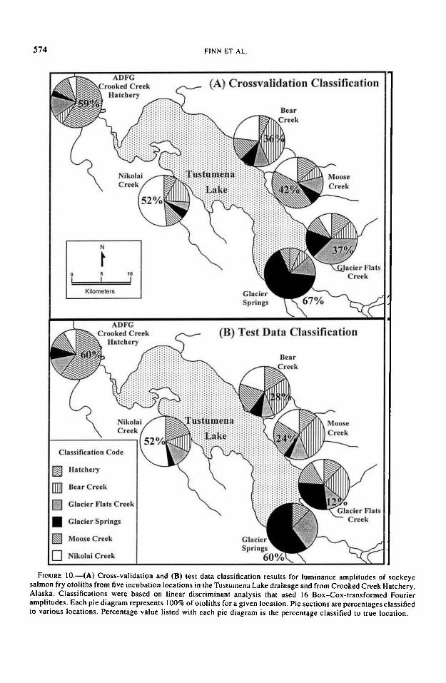
(Table 3). Total classification rates for test datawere 36.0-39.3%, and individual location classi-fications ranged from 12.0 to 64.0% (Table 3).None of the pairwise comparisons indicated sig-nificant differences in the cross-validation (Mc-Nemar's test; \z\ < 0.84, P > 0.20) or test dataclassification rates (McNemar's test; |z| ̂ 1.50, P> 0.06).

Quadratic discriminant analysis.—Total averagecross-validation classification rates appeared to berelatively stable through the 40- to 10-amplitudemodels (Figure 9b), ranging from 0.243 to 0.473.Increases in the classification rate were primarilydue to improvement in the rates for Glacier Springsand Moose Creek.

The three highest classifications occurred withthe 11- (44.7%), 14- (46.2%), and 15-amplitude(45.5%) models (Table 3). The covariance matriceswere significantly different for all three models(Bartlett's log-likelihood ratio; P < 0.001). Rangesfor cross-validation rates for individual locationswere 45.4: 54.6% for hatchery, 45.9-47.8% forBear Creek, 41.0-42.4% for Glacier Flats Creek,50.0-58.3% for Glacier Springs, 25.0-28.8% forMoose Creek, and 47.2-50.0% for Nikolai Creek(Table 3). Test data total classification ranged from34.7% to 40.7%, and ranges for individual locationmaximum classifications were 44.0-48.0% forhatchery, 28.0% for Bear Creek, 40.0-48.0% forGlacier Flats Creek, 36.0-48.0% for GlacierSprings, 16.0-28.0% for Moose Creek, and36.0-44.0% for Nikolai Creek (Table 3). Com-parisons among the three models did not result in

570 FINN ET AL.

0.0 0.25 0.50 0.75

Posterior Probability

FIGURE 7.—Distributions (based on cross-validationof posterior probabilities) of otoliths classified to hatch-ery origin for six groups of sockeye salmon fry fromTustumena Lake, Alaska. Probabilities were based onquadratic discriminant analysis that used, Box-Cox-iransformed Fourier amplitudes 8, 9, 16, 17, 22, 23, 24,25, 26, 80, and 88. Labels indicate true origin, n\ =number classified as hatchery; n-± - number classifiedas wild. Observations falling to right of vertical dashedline (0.5 probability level) were classified as hatchery-origin fish.

an obvious "best" model. Total cross-validation(McNemars test; |z| < 0.805, P > 0.21) and testdata (\z\ ̂ 1.67, P > 0.047) classification ratesdemonstrated no significant differences.

LDF and QDF model comparisons.—Both LDFand QDF resulted in three equivocal models. Ofthe LDF models, we selected the 16-amplitudemodel (LDF 16) for comparison because it resultedin maximum cross-validation and test data clas-sification rates (Table 3). Of the QDF models, the14-amplitude model (QDF 14) resulted in the high-est cross-validation classification but the lowesttest data classification (Table 3). On the other hand,the 11-amplitude model (QDF11) resulted in thelowest cross-validation classification but the high-est test data classification. When the LDF16 modelwas compared with the QDF models there were

no significant differences in the cross-validation(McNemar's test; |z| < 0.77, P > 0.22) or test data(McNemar's test; |z| < 1.02, P > 0.15) classifi-cation rates. Huberty (1994) suggested that a linearclassification may provide greater across-samplestability when the sample-to-discriminant-variableratio (Ni/p) is small or moderate, although no guid-ance was given for the definition of small. Huberty(1994) cautioned that such generalizations werebased on the m = 2 group case. Given the apparentequality of the classification success of the LDF 16and QDF models and the potential for higher sta-bility of the linear rule, we chose the LDF16 modelfor further examination.

Given that there were six groups, and under theassumption of equal probability of classification,the probability of an individual being assigned toany one location was 1/6. Although the classifi-cation rates for m = 6 groups were considerablylower than for m = 2 (i.e., hatchery-wild classi-fication), cross-validation classifications of indi-viduals to their true location occurred at a higherprobability than would be expected by chance (z> 4.9, P < 0.0001; Figure 10A). Test data clas-sifications of otoliths were significantly greaterthan chance for hatchery (z > 5.81, P ^ 0.0001),Glacier Springs (z > 5.81, P < 0.0001), and Ni-kolai Creek (z > 4.74, P < 4.74, P < 0.0001)(Figure 10B). Bear Creek (z = 1.52, P > 0.064),Glacier Flats Creek (z = -0.63, P > 0.266), andMoose Creek (z = 0.98, P > 0.163) test data clas-sifications were not significant (Figure 10B).Therefore, the otolith banding patterns as mea-sured by the selected Fourier amplitudes all con-tained some degree of location-specific informa-tion.

DiscussionOur analyses of otolith banding patterns repre-

sent a first attempt to use Fourier analysis to de-scribe discriminant variables based on luminanceprofiles. The Fourier amplitudes provide contin-uous variables for statistical discriminant analysis,and our methods of feature extraction were re-peatable and robust. High correct classificationrates (cross-validation 83%, test data 73%) wereachieved between hatchery and wild sockeye salm-on with quadratic discriminant analysis that used10 Box-Cox-transformed Fourier amplitudes (Ta-ble 2). We were pleased with our efforts to dis-criminate among various wild fry (m = 6 group),even though overall classification rates were below50% (Table 3), because we did find that site-spe-


0.60

0.40

0.20

0.00

-0.20 .

-0.40

-0.60

0.082"8 " 41' ' ' 5 4 ' 81 95 108 122 135 1< 9

0.06

0.04

0.02

0

-0.02

-0.04

-0.06

-008 •

-0.128 54 68 81 95 108 122 135 149

Distance (urn)

FIGURE 8.—(A) Mean standardized luminance profiles from Tustumena Lake, Alaska, hatchery and wild sockeyesalmon fry otoliths and (B) reconstruction of mean standardized hatchery and wild sockeye salmon fry otolithluminance profiles based on Fourier harmonics associated with amplitudes (8, 9. 16, 17, 23. 24, 25, 26, 80, and88) used in quadratic discriminant analysis. The wild group included otoliths from fry from Bear Creek, GlacierFlats Creek, Glacier Springs, Nikolai Creek, and Moose Creek.

cific information was indeed contained within thebanding patterns.

In almost all cases, test data classifications werelower than the cross-validation results. Althoughintuitively the lest data assessments should providethe most realistic estimate of true classificationrates, test data results can be highly variable withsmall sample sizes (Huberty 1994). Therefore, wethink that test data results should be viewed as aconservative measure of classification success,particularly in our rn = 6 group assessment (in-dividual group sample sizes = 25).

Otolith banding patterns formed during incu-bation have several desirable qualities for stockdiscrimination. For sockeye salmon, it is relativelyeasy to collect progeny of known-origin spawnersas they migrate from incubation to rearing envi-ronments. Also, subsequent growth and environ-mental conditions should not affect banding pat-terns formed during incubation (Campana andNeilson 1985). Unlike these banding patterns, theuse of otolith or shape analysis to discriminateamong wild populations is limited because highest

levels of correct classification seem to be associ-ated with growth rate differences or temporal andspatial separation of populations (Casselman et al.1981; Capana and Casselman 1993). For example,otolith shape analysis of populations of Atlanticsalmon Salmo salar from the United States, Can-ada, Ireland, and Britain resulted in highest correctclassification rates (84-91%) between continentsand lowest among samples analyzed from withineither North America (62-69%) or Europe (64-73%). Campana and Casselman (1993), who foundreasonable classification rates among populationsof Atlantic cod Gadus morhua of different growthrates, but poor classification when similar growthrates existed, suggest that population discrimina-tion based on otolith shape depends not only ondifferential growth rates, but on consistency of theenvironment over the lifetime of fish in a popu-lation. Therefore, if our purpose is to determinegrowth or survival differences among comingledgroups, characteristics formed during incubation,such as banding patterns, have a higher potentialfor utility than otolith shape characteristics.

572 FINN ET AL.

0.80

0.70

0.60

0.50

0.40

0.30

0.20

0.10

0.00

Number Of Amplitudes In Analysis43 41 39 37 35 33 31 29 27 25 23 21 19 17 15 13 11 9 7 5 3 1

Total. Nikolai Creek. Moose Creek ..... Hatchery, Glacier Springs

8C3

uo

fe(/>2u

none 92 31 88 65 12 25 85 3 100 47 10 38 127 23 27 95 16 33 28 30 967 8 125 21 26 6 53 1 73 115 124 102 18 54 11 117 123 24 90 15 22 (2)

51 49 47 45 43 41 39 37 35 33 31 29 27 25 23 21 19 17 15 13 11 9 7 5 3 1

0.00- ' i' i' i' i' i ' i' i » \ ' i » i » i « i • \ * i » i » i ' i * i » > • » » i » i ' i » i • i • i' i • inone 12 36 33 102 25 30 115 73 95 104 63 26 21 6 82 9 79 23 47 15 125 3 66 1 1 1

94 84 83 31 5 81 90 92 70 27 16 97 38 86 48 88 103 24 80 22 60 10 28 8 85Fourier Amplitude Dropped From Analysis

(2)

FiciURK 9.—Cross-validation classification rates (proportion correctly classified) for (A) linear (LDF) and (B) quadratic(QDF) discriminant function analysis on Box-Cox-transformed amplitudes from six groups of sockeye salmon fry otoliths,Tustumena Lake. Alaska. 1992. Initial LDF model included 43 amplitudes selected by stepwise discriminant analysis.Init ial QDF model included 51 amplitudes found to be significantly different (analysis of variance: P < 0.01) betweenhalchery and wild fry otoliths. At each analysis an additional amplitude was dropped (lower .r-axes). Upper .v-axesindicate number of amplitudes used for each analysis. Number in parentheses (lower axes, extreme right) indicatesamplitude retained in final model. Vertical dashed line indicates the w/3 = 17 variable model.

Few studies are available to compare our hatch-ery versus wild otolith classification rates. Al-though induced thermal banding results in 100%marking (Volk et al. 1990), we are unaware offindings that demonstrate the rate at which inducedmarks are recognized from admixtures of hatcheryand wild otoliths. Using oxytctracycline (OTC)validation, Paragamian et al. (1992) determinedthat the presence of hatch and check marks andincrement counts allow researchers to distinguishbetween hatchery and wild kokanee (a nonanad-

romous form of sockeye salmon). However, noclassification rate for hatchery otoliths not markedwith OTC was reported. Hendricks et al. (1994)used hatch and stocking checks as well as incre-ment counts to achieve a total classification rateof 89% for hatchery and wild American shad Alosasapidissima. These classifications were based onthe ability of trained observers to recognize hatch-ery versus wild patterns and not on statistical clas-sification.

Although we were unable to confidently sepa-

OTOL1TH DISCRIMINATION OF SOCKEYF. SALMON 573

TABLE 3.—Linear (LDF) and quadratic discriminant function (QDF) cross-validation and test data numbers (percent)of Tustumena Lake, Alaska, sockeye salmon otoliths correctly classified to true location for hatchery and five wildgroups based on Box-Cox-transformed Fourier amplitudes. (Actual numbers are the true numbers of individuals froma given location.)

Number ofamplitudes3-** Hatchery Bear Creek Glacier Flats Glacier Springs Moose Creek Nikolai Creek Total

LDF Cross-validation classification141617

Actual number

65 (59.09)65 (59.09)66 (60.00)

110

54 (34.39)57 (36.31)55 (35.03)

157

475251

(33.81)(37.41)(36.69)139

38 (63.33)40 (66.67)38 (63.33)

60

242223

(46.15)(42.31)(44.23)

52

585656

(53.70)(51.85)(51.85)108

286 (45.69)292 (46.65)289(46.17)

626

LDF test data classification141617

Aetual number

13(52.00)15 (60.00)15 (60.00)

25

57

(20.00)(28.00)

6 (24.00)25

333

(12.00)(12.00)(12.00)

25

14 (56,00)15 (60.00)16 (64.00)

25

5 (20.00)6 (24.00)6 (24.00)

25

141312

(56.00)(52.00)(48.00)

25

54 (36.00)59 (39.33)58 (38.67)

150

QDF cross-validation classification111415

Actual number

50 (45.45)60 (54.55)53 (48.18)

110

727575

(45.86)(47.77)(47.77)157

575759

(41.01)(41.01)(42.45)139

QDF test dataI I1415

Actual numbera Amplitudes used

14: 2. 9, 15. 16.16: 2.9, 11, 15.

12(48.00)1 1 (44.00)12 (48.00)

25

in LDL models,22. 24. 27. 28.16. 22. 23. 24.

777

30

(28.00)(28.00)(28.00)

25

33, 90, 95,28. 30, 33.

121012

117. . ..

(48.00)(40.00)(48.00)

25

m

35 (58.33)30 (50.00)32 (53.33)

60

classification12 (48.00)1 1 (44.00)9 (36.00)

25

151314

744

(28.85)(25.00)(26.92)

52

(28.00)(16.00)(16.00)

25

515452

I I

(47.22)(50.00)(48.15)108

(44.00)9 (36.00)

10 (40.00)25

280 (44.73)289(46.17)285 (45.53)

626

61 (40.67)52 (34.67)54 (36.00)

150

90,95, 117, 12317: 2. 9, I I . 15. 16. 22. 23. 24. 27. 28, 30. 33, 54, 90, 95, 117. 123

h Amplitudes used in QDF models.I I : 1. 2, 3. 8. 10. 11. 28. 60. 66. 85. 12514: I. 2. 3. 8, 10. 11. 15, 22. 28. 47. 60, 66. 85, 12515: I , 2, 3. 8, 10, 1 I T 15, 22. 28. 47. 60, 66. 80. 85, 125

rate the various wild groups of sockeye salmon inour study (m = 6), we found that site-specific in-formation was available within the otolith micro-structure formed during incubation. For all wildsamples, the cross-validation probability of an in-dividual being classified to its true incubation lo-cation was significantly greater than chance (Fig-ure 10A). These are differences among incubationsites that are less than 10 km apart, a result thatsuggests we may eventually be able to separatestocks after they have migrated into the commonrearing environment. Unlike our otolith method,pattern analysis of scales has been restricted todiscriminating freshwater origins of Pacific sal-monid populations on a relatively broad geograph-ic scale (Rowland 1969; Cook and Lord 1977;Cook 1982; Cross et al. 1987), because scales (un-like otoliths) form after emergence from incuba-tion environments. In addition to our otolith meth-od, however, emerging genetic and behavioralstudies show the existence or potential for within-

drainage diversity (Allcndorf and Waples 1995;Burger et al. 1995).

Temporal, spatial, and genetic differences in thedistributions of sockeye salmon spawning withinthe Tustumena Lake drainage have been docu-mented. Spawning occurs over a period longerthan 30 d, and adults entering lake tributariesspawn significantly earlier than sockeye salmonspawning along the lake's shoreline or outlet (Bur-ger et al. 1995). These differences appear to havea genetic basis (C. Burger, unpublished data). Oth-er differences include the distances over whichspawning occurs in Tustumena Lake tributaries(Nikolai Creek, >20 km; Bear and Moose creeks,>10 km; Glacier Flats Creek, <4 km) and thevariation suggested by significant differences infry lengths (Figure 4), degree of development(yolk sac absorption), and frequency of feeding(Finn 1995).

The ecological differences among sockeyesalmon that spawn and incubate in the Tustumena

574 FINN ET AL.

(A) Crossvalidation Classification

BearCreek

ADFGCrooked Creek

Hatchery

(B) Test Data Classification

BearCreek

ADFGCrooked Creek

Hatchery

Hatchery

Bear Creek

Glacier Flats Creek

Glacier Springs

Moose Creek

Nikolai Creek

Glacier!Springs

60%VFIGURE 10.—(A) Cross-validation and (B) test data classification results for luminance amplitudes of sockeye

salmon fry otoliths from five incubation locations in the Tustumena Lake drainage and from Crooked Creek Hatchery,Alaska. Classifications were based on linear discriminant analysis that used 16 Box-Cox-transformed Fourieramplitudes. Each pie diagram represents 100% of otoliths for a given location. Pie sections are percentages classifiedto various locations. Percentage value listed with each pie diagram is the percentage classified to true location.


Lake drainage are undoubtedly a factor in the clas-sification rates we achieved with Fourier analysis.Although our best classification rate occurred be-tween groups incubating in substantially differentenvironments (hatchery versus wild), we achievedrates among wild groups that exceeded those ex-pected by chance alone and that appear to reflectsite-specific information. The temporal and spatialdifferences exhibited by Tustumena Lake sockeyesalmon are small in comparison with those ob-served in other parts of the species' range wherespawning and fry outmigration can be quite pro-tracted (Card et al. 1987; Burgner 1991). It shouldbe noted that our study is limited to a single, geo-logically young drainage that is thought to be un-dergoing population differentiation (Burger et al.1995).

An area for improvement in our approach is inthe selection of variables. The looping procedurewe used did not include all possible subsets ofamplitudes. Once an amplitude was removed (e.g.,deleted at the p = 15 amplitudes step) it was notreevaluated at smaller p subsets. The plots of clas-sification rates that were generated during thelooping procedures did not result in clearly definedmaxima. Indeed, discrimination among both m =2 and m = 6 groups resulted in equivocal models.Further work is necessary to develop and applyalgorithms that will evaluate all possible subsetsof p amplitudes to improve the discriminant ca-pabilities of the present method (Huberty 1994),not only to improve discrimination, but to allowresearchers to concentrate on amplitude subsetsthat meet variable-to-sample ratio criteria (Wil-liams and Titus 1988). Furthermore we have ap-plied only two very similar discrimination tech-niques (LDF and QDF) to these data.

Although our method for transect placement andlength was developed to provide a means for stan-dardization that was independent of ambiguousreference points, the use of a standard length tran-sect may have introduced some degree of con-founding variability. If differential developmentrates exist, then one would expect that the periodof time covered by a standard length transect willvary from otolith to otolith. We are not able at thistime to estimate what sort of effect this may havehad on our results. It should also be noted that ouranalysis was limited to otoliths from young-of-the-year fry. Although otolith banding patterns arti-ficially induced during incubation are identifiablein adult otoliths (Volk 1990), it is as yet unprovedwhether the level of otolith band discriminationwe used on fry would be feasible with adult fish

otoliths. It is also not known what factors otherthan temperature (e.g., genetics) may influence thebanding patterns we observed.

Our study represents the first use of Fourieranalysis to describe differences in otolith bandingpatterns. Although our method needs refinementto determine the final degree to which the variouswild sockeye salmon fry within Tustumena Lakecan be separated, the present study indicates thepotential to discriminate phenotypic differences insockeye salmon otoliths that develop during in-cubation. With further research and application ofimage analysis, the examination of otolith bandingpatterns formed during incubation could providediscrimination that would allow within-drainageestimation of population parameters (e.g., mortal-ity and growth functions) for various groups ofhatchery-produced and wild sockeye salmon fryduring their freshwater residence.

AcknowledgmentsWe thank R. Wilmot (National Marine Fisheries

Service) and J. Reynolds, R. Barry, J. Collie, andL. Haldorson (University of Alaska) for their ad-vice and support throughout this study. B. Rieman(U.S. Forest Service) and E. Knudsen (U.S. Gel-ogical Survey) provided useful comments on themanuscript. G. Sonnevil (U.S. Fish and WildlifeService) and his staff provided logistical supportthat facilitated completion of this project. AlaskaDepartment of Fish and Game personnel also pro-vided assistance, especially R. Och, D. Schmidt,and P. Shields. K. Cash, D. Dawley, K. Hensel,and D. Nelson assisted with collection of field data.

ReferencesAdams, N., and five coauthors. 1994. Variation in mi-

tochondrial DNA and allozymes discriminates earlyand late forms of chinook salmon (Oncorhynchustshawytscha) in the Kenai and Kasilof rivers, Alas-ka. Canadian Journal of Fisheries and Aquatic Sci-ences 51 (Supplement 1):172-181.

Allendorf, F. W., and R. S. Waples. 1995. Conservationand genetics of salmonid fishes. Pages 238-280 inJ. C. Avise and J. L. Hamrick, editors. Conservationgenetics: case histories from nature. Chapman andHall, London.

Bird, J. L., D. T. Eppler, and D. M. Checkley. 1986.Comparisons of herring otoliths using Fourier seriesshape analysis. Canadian Journal of Fisheries andAquatic Sciences 43:1228-1234.

Blair, G. R.. and T. P. Quinn. 1991. Homing and spawn-ing site selection by sockeye salmon (Oncorhynchusnerka) in Iliamna Lake, Alaska. Canadian Journalof Zoology 69:176-181.

Brothers, E. B. 1990. Otolith marking. Pages 183-202i/i Parker et al. (1990).

576 FINN ET AL.

Burger, C. V., J. E. Finn, and L. Holland-Bartels. 1995.Pattern of shoreline spawning by sockeye salmonin a glacially turbid lake: evidence for subpopula-tion differentiation. Transactions of the AmericanFisheries Society 124:1-15.

Burgner, R. L. 1991. Life history of sockeye salmon(Oncorhynchus nerka). Pages 1-117 in C. Groot andL. Margolis, editors. Pacific salmon life histories.University of British Columbia Press, Vancouver.

Butler. J. L. 1992. Collection and preservation of ma-terial for otolith analysis. Pages 13-17 in D. K.Stevenson and S. E. Campana. editors. Otolith mi-crostructure and examination and analysis. Cana-dian Special Publication of Fisheries and AquaticSciences 117.

Campana, S. E., and J. M. Casselman. 1993. Stock dis-crimination using otolith shape analysis. CanadianJournal of Fisheries and Aquatic Sciences 50:1062-1083.

Campana, S. E., and J. D. Neilson. 1985. Microstructurein fish otoliths. Canadian Journal of Fisheries andAquatic Sciences 42:1014-1032.

Casselman, J. M., J. J. Collins, E. J. Crossman, P. E.Ihssen, and G. R. Spangler. 1981. Lake whitefish(Coregonus clupeaformis) stocks of the Ontario wa-ters of Lake Huron. Canadian Journal of Fisheriesand Aquatic Sciences 38:1772-1779.

Castonguay. M., P. Simard, and P. Gagnon. 1991. Use-fulness of Fourier analysis of otolith shape for At-lantic mackerel (Scomber scombrus) stock discrim-ination. Canadian Journal of Fisheries and AquaticScience 48:296-302.

Cook, R. C. 1982. Stock identification of sockeye salm-on (Oncorhynchus nerka) with scale pattern rec-ognition. Canadian Journal of Fisheries and AquaticSciences 39:611-617.

Cook, R. C.. and G. E. Lord. 1977. Identification ofslocks of Bristol Bay sockeye salmon, Oncorhyn-chus nerka, by evaluating scale patterns with a poly-nomial discriminant method. U.S. National MarineFisheries Service Fishery Bulletin 76:415-423.

Cross, B. A., W. F. Goshert, and D. L. Hicks. 1987.Origins of sockeye salmon in the fisheries of upperCook Inlet, 1984. Alaska Department of Fish andGame, Technical Fishery Report 87-01, Juneau.

Currens, K. P., C. B. Schreck, and H. W. Li. 1988. Re-examination of the use of otolith nuclear dimensionsto identify juvenile anadromous and non-anadro-mous rainbow trout, Salmo gairdneri. U.S. NationalMarine Fisheries Service Fishery Bulletin 86:160-163.

Daniel, W. W. 1990. Applied nonparametric statistics.PWS-Kent, Boston.

Finn, J. E. 1995. Fourier analysis of otolith bandingpatterns to discriminate among hatchery, tributary,and lake shore incubated sockeye salmon (Onco-rhynchus nerka) juveniles in Tustumena Lake, Alas-ka. Master's thesis. University of Alaska, Fairbanks.

Friedland. K. D., and D. G. Reddin. 1994. Useofotolithmorphology in stock discriminations of Atlanticsalmon (Salmo salar). Canadian Journal of Fisheriesand Aquatic Sciences 51:91-98.

Card, R., B. Drucker, and R. Fagen. 1987. Differenti-ation of subpopulations of sockeye salmon (Onco-rhynchus nerka), Karluk River System, Alaska. Ca-nadian Special Publication of Fisheries and AquaticSciences 96:408-418.

Gharrett, A. J., S. Lane, A. J. McGregor, and S. G. Tay-lor. In press. Use of a genetic marker to examinegenetic interaction among subpopulations of pinksalmon (Oncorhynchus gorbuscha). Canadian Spe-cial Publication of Fisheries and Aquatic Sciences.

Gonzalez. R. C., and P. Wintz. 1987. Digital imageprocessing. Addison-Wesley, Reading, Massachu-setts.

Hendricks, M. L., T. R. Bender, Jr., and V. A. Mudrak.1991. Multiple marking of American shad with tet-racycline antibiotics. North American Journal ofFisheries Management 11:212-219.

Hendricks, M. L.. D. L. Torsello. and T. W. H. Backman.1994. Use of otolith microstructure to distinguishwild from hatchery-reared American shad in theSusquehanna River. North American Journal ofFisheries Management 14:151-161.

Holland-Bartels, L., C. V. Burger, and S. Klein. 1994.Studies of Alaska's wild salmon stocks: some in-sights for hatchery supplementation. Transactionsof the North American Wildlife and Natural Re-sources Conference 59:244-253.

Huberty, C. J. 1994. Applied discriminant analysis. Wi-ley series in probability and mathematical statistics.Wiley, New York.

Ihssen, P. E., and five coauthors. 1981. Stock identifi-cation: materials and methods. Canadian Journal ofFisheries and Aquatic Sciences 38:1838-1855.

Jarvis, R. S., H. F. Klodowski, and S. P. Sheldon. 1978.A new method of quantifying scale shape and anapplication to stock identification in walleye (Stizo-stedion vitreum vitreum). Transactions of the Amer-ican Fisheries Society 107:528-534.

Jewell, E. D., and R. C. Hager. 1972. Field evaluationof coded wire tag detection and recovery tech-niques. Pages 183-190 in R. C. Simon and P. A.Larkin, editors. The stock concept in Pacific salmon.H. R. MacMillan Lectures in Fisheries, Universityof British Columbia, Vancouver.

Johnson, R. A., and D. W. Wichern. 1988. Applied mul-tivariate statistical analysis. Prentice-Hall, Engle-wood Cliffs, New Jersey.

Kyle, G. B. 1992. Summary of sockeye salmon (On-corhynchus nerka) investigations in TustumenaLake, 1981-1991. Alaska Department of Fish andGame, Fishery Rehabilitation and Enhancement Di-vision Report 122. Juneau.

Lane, S., A. J. McGregor, S. G. Taylor, and A. J. Ghar-rett. 1990. Genetic marking of an Alaskan pinksalmon population, with an evaluation of the markand marking process. Pages 395-406 in Parker etal. (1990).

Marshall, S. L., and S. S. Parker. 1982. Pattern iden-tification in the microstructure of sockeye salmon(Oncorhynchus nerka) otoliths. Canadian Journal ofFisheries and Aquatic Sciences 39:542-547.

McKern, J. L., H. F. Horton, and K. V. Koski. 1974.


Development of steelhead trout (Salmo gairdneri)otoliihs and their use for age analysis and for sep-arating summer from winter races and wild fromhatchery stocks. Journal of the Fisheries ResearchBoard of Canada 31:1420-1426.

McLachlan, G. J. 1992. Discriminant analysis and sta-tistical pattern recognition. Wiley series in proba-bil i ty and mathematical statistics. Wiley, New York.

Mulligan, T. J., F. D. Martin, R. A. Smucker, and D. A.Wright. 1987. A method of stock identificationbased on the elemental composition of striped bassMorone saxatilis (Walbaum) otoliths. Journal of Ex-perimental Marine Biology and Ecology 114:241-248.

Nielsen, L. A. 1992. Methods of marking fish and shell-fish. American Fisheries Society, Special Publica-tion 23, Bethesda. Maryland.

Neilson, J. D. 1992. Sources of error in otolith micro-structure examination. Pages 115-125 in D. K. Ste-venson and S. E. Campana. editors. Otolith micro-structure examination and analysis. Canadian Spe-cial Publication of Fisheries and Aquatic Sciences117.

Neilson, J. D., and G. H. Geen. 1982. Otoliths of chi-nook salmon (Oncorhynchus tshawyischa): dailygrowth increments and factors influencing their pro-duction. Canadian Journal of Fisheries and AquaticSciences 39:1340-1347.

Neilson, J. D.. and G. H. Geen. 1984. Effects of feedingregimes and diel temperature cycles on otolith in-crement formation in juvenile chinook salmon. On-corhynchus tshawytscha. U.S. National Marine Fish-eries Service Fishery Bulletin 83:91-101.

Neilson, J. D., G. H. Geen. and D. Bottom. 1985a. Es-luarine growth of juvenile chinook salmon (Onco-rhynchus ishawytscha) as inferred from otolith mi-crostructure. Canadian Journal of Fisheries andAquatic Sciences 42:899-908.

Neilson, J. D., G. H. Geen, and B. Chan. I985b. Vari-ability in dimensions of salmonid otolith nuclei: im-plications for stock identification and microstruc-lure interpretation. U.S. National Marine FisheriesService Fishery Bulletin 83:81-89.

Pannella, G. 1971. Fish otoliihs: daily growth layersand periodical patterns. Science 173:1124-1127.

Pannella, G. 1980. Growth patterns in fish sagittae.Pages 519-560 in D. C. Rhoads and R. A. Lutz,editors. Skeletal growth of aquatic organisms. Ple-num Press, New York.

Paragamian, V. L., E. C. Bowles, and B. Hoclschcr.1992. Use of daily growth increments on otolithsto assess stockings of hatchery-reared kokanees.Transactions of the American Fisheries Society 121:785-791.

Parker, N. C., and five coeditors. 1990. Fish-markingtechniques. American Fisheries Society. Sympo-sium 7, Bethesda, Maryland.

Ricker, W. E. 1972. Heredity and environmental factorsaffecting certain salmonid populations. Pages 27-160 i/i R. C. Simon and P. A. Larkin, editors. Thestock concept in Pacific salmon. H. R. MacMillan

Lectures in Fisheries, University of British Colum-bia, Vancouver.

Rieman, B. E., D. L. Myers, and R. L. Nielsen. 1994.Use of otolith microchemistry to discriminate On-corhynchus nerka of resident and anadromous ori-gin. Canadian Journal of Fisheries and Aquatic Sci-ences 51:68-77.

Riley, L. M., and R. F. Carline. 1982. Evaluation ofscale shape for the identification of walleye stocksfrom western Lake Erie. Transactions of the Amer-ican Fisheries Society 111:736-741.

Rowland, R. G. 1969. Relationship of scale character-istics to river of origin in four stocks of chinooksalmon (Oncorhynchus tshawytscha) in Alaska. U.S.Fish and Wildlife Service Special Scientific Report-Fisheries 577.

Rybock, J. T., H. F. Morion, and J. L. Fessler. 1975. Useof otoliths to separate juvenile steelhead trout fromjuvenile rainbow trout. U.S. National Marine Fish-eries Service Fishery Bulletin 73:654-659.

SAS Institute. 1989a. SAS/STAT user's guide, version6, 4th edition, volume I . SAS Institute, Cary. NorthCarolina.

SAS Institute. 1989b. SAS/STAT user's guide, version6, 4th edition, volume 2. SAS Institute, Cary. NorthCarolina.

Secor, D .H. , J ,M. Dean, and E.H.Luben. 1992. Ololithremoval and preparation for microanalysis. Pages19-57 in D. K. Stevenson and S. E. Campana, ed-itors. Otolith microstructure examination and anal-ysis. Canadian Special Publication of Fisheries andAquatic Sciences 117.

Seeb, L. W.. J. E. Secb, R. L. Alien, and W. K. Hersh-berger. 1990. Evaluation of adult returns of ge-netically marked chum salmon, with suggested fu-ture applications. Pages 418-425 in Parker et al.(1990).

Smoker, W. W., A. J. Gharrett, and M. S. Stekol. In press.Genetic variation in the timing of anadromous mi-gration within a spawning season in a populationof pink salmon. Canadian Special Publication ofFisheries and Aquatic Sciences.

Sokal, R. R., and F. J. Rohlf. 1981. Biometry, 2nd edi-tion. Freeman, San Francisco.

SYSTAT. 1992. SYSTAT for windows: statistics, ver-sion 5 edition. SYSTAT, Evanston, Illinois.

Taylor, E. B. 1991. A review of local adaptation inSalmonidae, with particular reference to Pacific andAtlantic salmon. Aquaculture 98:185-207.

Volk, E. C., S. L. Schroder, and K. L. Fresh. 1990.Inducement of unique otolith banding patterns as apractical means to mass-mark juvenile Pacific salm-on. Pages 203-215 in Parker el al. (1990).

Volk, E. C., R. C. Wissmar, C. A. Simenstad, and D. M.Eggers. 1984. Relationship between otolith micro-structure and growth of juvenile chum salmon (On-corhynchus keta) under different prey rations. Ca-nadian Journal of Fisheries and Aquatic Sciences41:126-133.

Williams, B. K., and K. Titus. 1988. Assessment ofsampling stability in ecological applications of dis-criminant analysis. Ecology 69:1275-1285.

578 FINN ET AL.

Wilmot, R. L., and C. V. Burger. 1985. Genetic differ-ences among populations of Alaskan sockeye salm-on. Transactions of the American Fisheries Society114:236-243.

Wilmot, R. L., and five coauthors. 1994. Genetic stockstructure of western Alaska chum salmon and acomparison with Russian far east stocks. CanadianJournal of Fisheries and Aquatic Sciences 51 (Sup-plement l):84-94.

Wilson, K. H., and P. A. Larkin. 1982. Relationship

between thickness of daily growth increments insagittae and change in body weight of sockeye salm-on (Oncorhynchus nerkd). Canadian Journal of Fish-eries and Aquatic Sciences 39:1335-1339.

Yamada, S. B., and T. J. Mulligan. 1990. Screening ofelements for the chemical marking of hatcherysalmon. Pages 550-561 in Parker et al. (1990).

Received February 28, 1996Accepted December 17, 1996

discrimination among populations of sockeye salmon fry with

Documents