direct titration for measurement of soil … titration for measurement of soil lime requirement and...

DIRECT TITRATION FOR MEASUREMENT OF SOIL LIME

REQUIREMENT AND INDIRECT LIME REQUIREMENT

ESTIMATION BY SOIL PROPERTIES

by

MIN LIU

(Under the direction of David E. Kissel, Ph. D)

ABSTRACT

Previous studies about the titration curves of acid soils reported a linear relationship in the approximate range 4.5 < pH(H2O) < 6.5. It appears possible to establish the slope of the titration curve with 3 aliquots of Ca(OH)2 and then predict the lime requirements (LRs) to pH 6.5. The objective of this study was to evaluate the possibility of developing a direct titration procedure to measure the LRs of acid soils for routine use in soil testing laboratories. Seventeen soil samples with a wide range of clay and soil organic carbon contents were collected from five of the major land resource areas of Georgia. A 30 minute interval time between additions was found to be relatively short but adequate for the base added to react with the soil acids. A 3-day Ca(OH)2 incubation study revealed that the 3-points prediction from the direct titration with 30 minute interval time between additions estimated approximately 80% of the soil acidity. To simplify the procedure, one dosing of Ca(OH)2 was also tried to establish the titration slope in both water and 0.01 M CaCl2. Although the 2-point titration in water was subject to errors, the two point prediction of the LRs in 0.01 M CaCl2 estimated approximately 83% of the soil acidity. The CaCO3 incubation was found to overestimate the LRs. The LRs were highly correlated with initial pH and total carbon content. INDEX WORDS: Titration, Lime requirement, Soil testing, Soil acidity




By

MIN LIU

B.S., China Agricultural University, 2001

A Thesis Submitted to the Graduate Faculty of The University of Georgia in Partial

Fulfillment of the Requirements for the Degree

MASTER OF SCIENCE

ATHENS, GEORGIA

2003

© 2003

Min Liu

All Rights Reserved




by

MIN LIU

Approved:

Major Professor: David E. Kissel

Committee: Miguel Cabrera Paul Vendrell

Electronic Version Approved:

Maureen Grasso Dean of the Graduate School The University of Geogia August 2003

iv

DEDICATION

This thesis is dedicated to my father, Mr. Dinghong, Liu and to my mother, Mrs.

Wanmei, He. God bless you.

v

ACKNOWLEGEMENTS

I would like to express my special thanks to Dr. David E. Kissel, my major professor,

for this guidance, patience and assistance in completion of this degree. The project would

not have been successful without his continued support and encouragement. I also thank

Dr. Miguel L. Cabrera and Dr. Paul Vendrell for serving as the committee members.

There were many other people who have assisted in different aspects of this project

during the past two years. I would thank Dr. Feng Chen, who has been a very good helper

and honest friend in many aspects of my foreign life here. Much appreciation is extended

to Wick Johnson for his patience on my endless questions and to Kim for her analysis of

the soil particle size distribution.

vi

TABLE OF CONTENTS

ACKNOWLEDGEMENTS �� ........ v

LIST OF TABLES ��.��....... xiii

LIST OF FIGURES ��.......... x

INTRODUCITON ��........ 1

LITERATURE REVIEW ��...... .......4

pH Determination and Measurement ��...... 4

pH Buffering Capacity ��...��......... 8

Lime Requirement Determination ��.......9

Incubation Methods ��...��........17

References ��...��..... .20

CHAPTER 1 DIRECT TITRATION FOR MEASUREMENT OF SOIL

LIME REQUIREMENT ��......... 25

Abstract ��............................................................................... ......25

Introduction ��..��........ .26

Materials and Methods ��..��....... 27

Results and Discussion ��..��,�� ......30

Conclusions ��.�.�...� ......34

vii

References ��..��. 45

CHAPTER 2 INTERPRETATION OF TITRATION CURVES ��..��.. 46

Abstract ��.�.. 46

Introduction ��..�.�.. 47

Materials and Methods ��.��..�. 48

Results and Discussion ��... 50

Conclusions ��. 53

References ��... 62

CHAPTER 3 CaCO3 INCUBATION METHODS REVISITED AND AN INDIRECT

LIME REQUIREMENT ESTIMATION BY

SOIL PROPERTIES ��...��. 63

Abstract ��...�� 63

Introduction ��...��.�. 64

Materials and Methods ��...��. 65

Results and Discussion ��...�� 68

References ��...�� 77

APPENDIX Fig. 1 Titration curves for twelve soils in water and 0.01 M CaCl2��.79

viii

LIST OF TABLES

Table 1.1 Selected physical and chemical properties of acid

soils used ��...�� 38

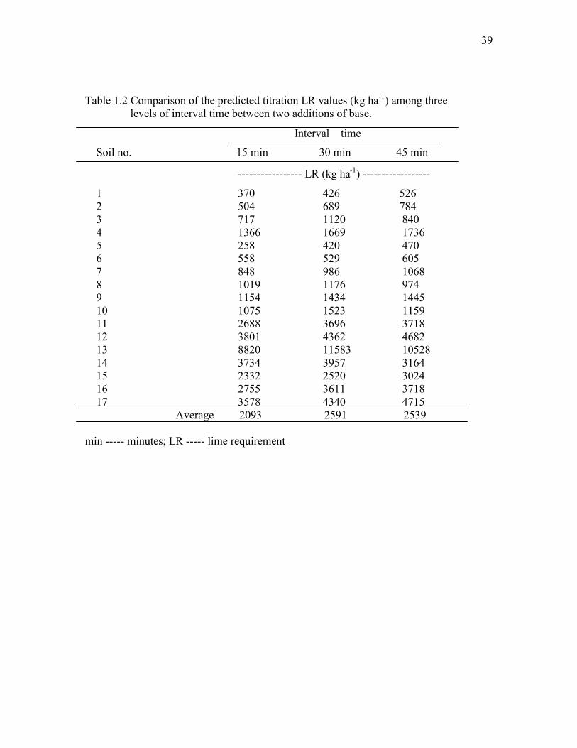
Table 1.2 Comparison of the predicted titration LR values (kg ha-1) among three

levels of interval time between two additions of base ��... 39

Table 1.3 Comparison of the LR values (kg ha-1) between titration curve and

prediction of its first 3 aliquots of base ��.�� 40

Table 1.4 The soil pH change during the 4-day incubation with standard

Ca(OH)2 Solution ��.��... 41


soils used ��55


soils used ��...�� 71

Table 3.2 Soil pH comparison between CaCO3 incubation and

Ca(OH)2 incubation ��..72

Table 3.3 Net H+ produced from N transformations in incubated

soils at day 60 �� 73

Table 3.4 Pearson correlation coefficients among physicochemical properties

of 17 soils and lime requirements (LR) �� 74

Table 3.5 GLM Table for the linear model of lime requirement (103 kg ha-1)

ix

relating to ∆pH and total carbon content (%) ��.�� 75

Table 3.6 GLM Parameter table for the linear model of lime requirement (103 kg ha-1)

relating to ∆pH and total carbon content (%) ��..��..��... 76

x

LIST OF FIGURES

Fig. 1.1 Location of Georgia soils selected for lime requirement study �� 36

Fig. 1.2 Example of LR Prediction from 3 aliquots of Ca(OH)2 with an interval time of

30 minutes between two additions, for soil No. 9��.��.. 37

Fig. 1.3 Relationship between Ca(OH)2 incubation LR values and predicted LR

values from the first 3 aliquots of Ca(OH)2 ��........... 42

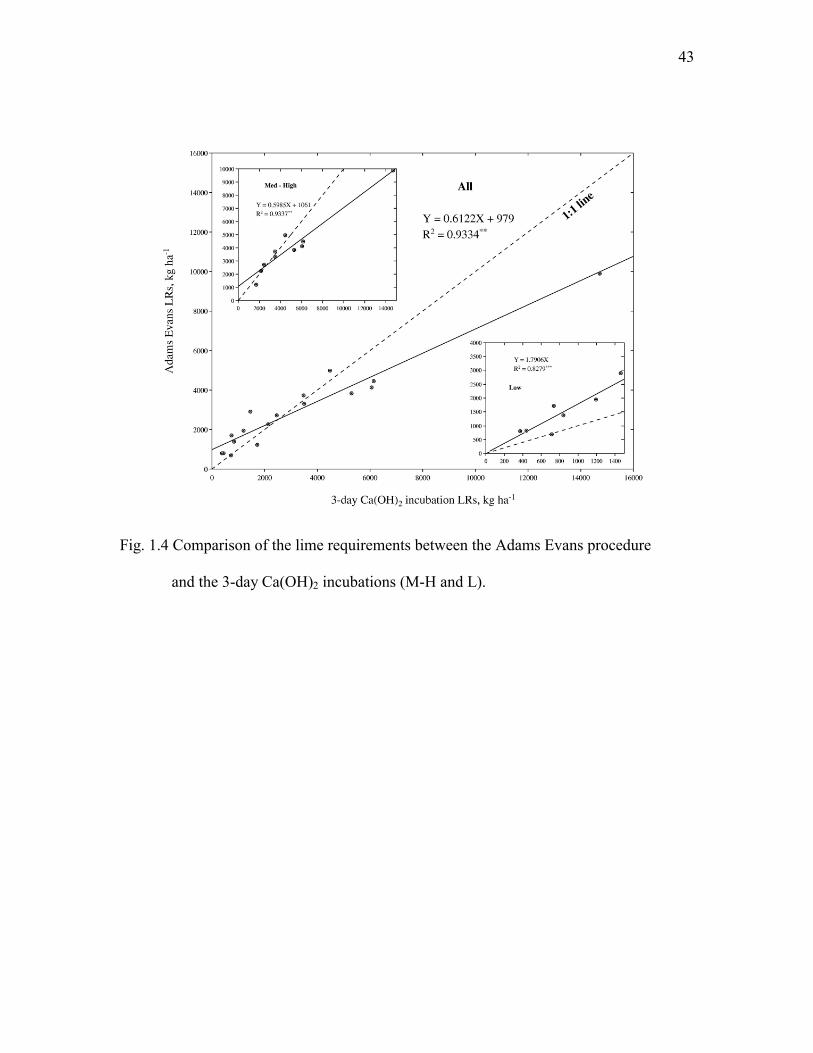
Fig. 1.4 Comparison of the lime requirements between the Adams Evans

procedure and the 3-day Ca(OH)2 incubations (M-H and L)�...��.. 43

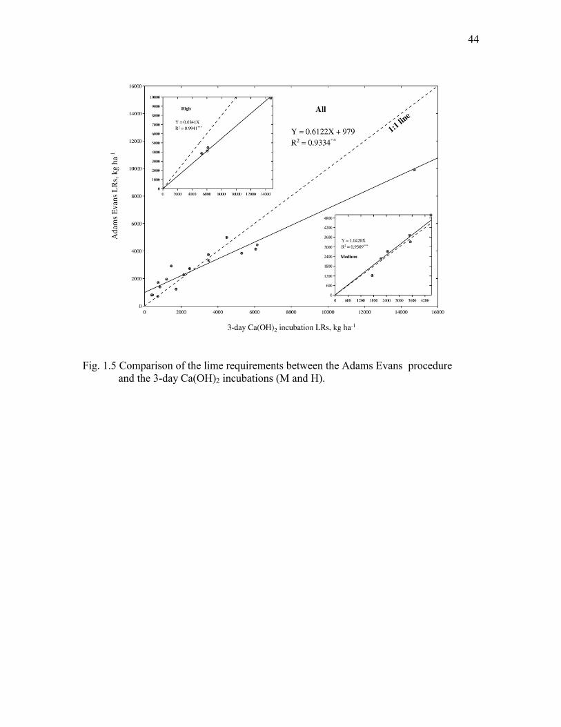
Fig. 1.5 Comparison of the lime requirements between the Adams Evans

procedure and the 3-day Ca(OH)2 incubations (M and H)��...��.. 44

Fig. 2.1 Titration curves for 5 soils in water and in 0.01 M CaCl2 ��.�� 56

Fig. 2.2 Slope comparison between water titration and 0.01 M CaCl2 titration ��...�.. 57

Fig. 2.3 Slope comparison between data points to pH 6.5 (no first point) and two

points (0 and 3 mL) in water titration ��..�.�� 58

Fig. 2.4 Comparison of titration slopes in 0.01 M CaCl2 determined by regression of all

data points vs slopes calculated from two points (0, 3 mL Ca(OH)2 ��. 59

Fig. 2.5 LR comparison between readings on water titration curves and calculations

from CaCl2 titration slope (0 and 3 mL) with initial pH in water �� 60

Fig. 2.6 LR comparison between 2 point prediction in 0.01 M CaCl2 titrations

and 3-day Ca(OH)2 incubation ��. 61

1

INTRODUCTION

The lime requirement (LR) is the amount of limestone needed to increase the pH of

the plow layer of acid soil to a desired level (McLean, 1970). Dunn (1943) studied direct

titration to predict the LR of acid soils and focused on the influence of equilibrium time

on the reaction between added base and soil acids. He found that four days were needed

for pH values to reach equilibrium when 0.022 M Ca(OH)2 solution was added to acid

soils. He also discovered that shaking affected the time required for soil pH values to

reach equilibrium. He reported that equilibrium was reached within eight hours with

shaking as compared to four days for the suspensions without shaking. Finally, he

suggested a standard direct titration method for lime requirement by incorporating acid

soils with different rates of 0.022 M Ca(OH)2 for four days. The Ca(OH)2 titration

method proposed by Dunn (1943) for measuring the LR was widely accepted as a

reliable method for estimating the LRs (Follett and Follett, 1980; Alabi et al, 1986;

McConell et al., 1990; Owusu-Bennoah et al., 1995). However, Dunn�s method was also

considered to be a time-consuming procedure and not suitable for routine use in soil

testing laboratories. Many studies focused on the titration curve itself. Magdoff and

Bartlett (1985) concluded that the relationship between pH and OH- added is nearly linear

within the pH range of most agricultural soils (4.5 to 6.5). Weaver (2002) also reported

an approximately linear relationship between pH and base added for a series of Georgia

soils.

2

The Adams-Evans (AE) buffer procedure (Adams and Evans, 1962) for predicting LR

is used widely in soil test laboratories in the south-east United States. However, it has

been reported to overestimate the LR (Follett and Follett, 1980; Tran and Lierop, 1981;

Alabi et al, 1986). Tran and Lierop (1981) also noted the limited range of the AE buffer

and its relatively poor precision, as indicated by the relatively low correlation coefficient

between estimates of LR from incubation and those using the AE procedure (r2 = 0.78**).

Another concern about the AE buffer is the potential toxicity from one of its components,

p-nitrophenol. Considering the inaccuracy and environmental concern of the AE buffer

procedure, the objectives of these studies were to evaluate the possibility of developing a

direct titration procedure to measure the LRs of acid soils for routine use in soil testing

laboratories.

Incubation methods with CaCO3 are also considered reliable to determine the lime

requirements of acid soils. They are often used as calibrations for buffer methods (Tran

and van Lierop, 1981; Loynachan, 1981; Barrow and Cox, 1990). Baker and Chae (1977)

reported that the use of room temperature incubation of incremental mixtures of CaCO3

and soil to determine lime requirements overestimates the actual lime requirements

determined by field testing. This occurs because soil acidity increases under room

temperature incubation. Incubation methods using CaCO3 are subject to some arbitrary

influences such as incubation time, moisture content, carbon dioxide levels, and air

pollutants (Alabi et. al. 1986).

Indirect LR-determination procedures rely on estimating a LR from soil properties

without directly measuring acidity. The indirect LR estimation procedure is advanced for

use when buffer-pH values are not available and a LR recommendation is needed. It is

3

fairly accurate and relies on common soil tests. Owusu-Bennoah et. al. (1995) related pH,

organic carbon, and clay with Ca(OH)2 incubated LR and found: LR (103 kg ha-1) = 4.2 �

1.1pH + 1.7(% organic carbon) + 0.05(% clay), R2 = 0.92.

4

LITERATURE REVIEW

pH Determination and Measurement

Sorensen(1909) defined pH as the negative logarithm of H+ concentration. This

notation has been maintained; though, H+ activity has replaced concentration to adapt it

to electromotive cell potentials. Soil pH is determined routinely with a glass combined

with a calomel reference electrode. It consists of measuring soil-solution electromotive

force (emf) and comparing it to defined buffer standard values. Accuracy depends on the

differences in the liquid junction-potential error between standards and sample. A soil pH

is determined by the activity of H+ in solution to which are added the influence of several

other factors. These are discussed under the following subheadings: A. soil/solution ratios

and sample size; B. soluble salts; C. suspension effect; D. carbonic acid; E. drying; and F.

seasonal pH fluctuation. Many of those factors are closely interrelated.

A. Soil/Solution Ratios and Sample Size

In early research, soil pH was typically measured at moisture contents approaching

those found in the field. However, both Huberty and Haas (1940) and Chapman et al.

(1941) found that soil pH varied from about 0.5 to 1.5 pH with changing moisture

contents. Water contents greater than those to produce a paste were required to ensure

stable and reproducible results (Chapman et al., 1941). The reasons for Chapman et. al.�s

observations are the following: 1, moisture content varies with sample texture and OM

5

content; 2, moisture content is often subjective; 3, low moisture contents aggravate

junction potential errors; 4, low moisture contents provide unreliable electrode-solution

contact; and 5, electrode malfunction and breakage risk are higher when inserting into a

paste. Peech (1965a) and McLean (1973) recommended a 1:1 soil/water ratio for

determining soil pH. Peech (1965a) also recommended a 20-g soil sample in 20 mL water

and concluded that soil pH, measured at a given soil/solution ratio is not affected by

sample size. Sixty soils samples were weighed out (Y) and scooped out (X) and then pHs

were determined in 1:1 soil/water ratio. pHs were in the range from 3.59 to 8.81(Y), and

3.56 to 8.79 (X) with means of 6.28 and 6.25, respectively (Y=1.01X +0.05; r=0.999**,

significant at P=0.01; sy.x=0.06), indicating a very close agreement and that weighing

was unnecessary for precise pH measurement. Schofield and Taylor (1955) originally

recommended that soil pH be measured in 0.01 M CaCl2 with a 1:2 soil/solution ratio.

Values are not sensitive to fairly wide changes in soil/solution ratio when measured in

0.01 M CaCl2 (Schofield & Taylor, 1955; Clark 1964; Ryti, 1965; White, 1969). Puri and

Asghar (1938) also reported using soil/1 N KCl ratios ranging from 1:2.5 to 1:25 and

found little effect on pH of acid soils, but a significant effect on that of calcareous soils.

Little, if any, dilution effect was reported between pH measurements made at 1:1 and 1:2

ratios with 0.01 M CaCl2 and 1 N KCl for mineral soils and Histosols by van Lierop and

Tran (1979) and van Lierop (1981), respectively. It is unnecessary, therefore, to weigh

soil samples for pH determination when using these solutions.

B. Soluble Salts and Lime Potential

The lime potential was defined as being: pH � 1/2p(Ca +Mg). Schofield and Taylor

(1955) found that soil pH and ½ p(Ca +Mg) increase in value with dilution but their

6

difference, the lime potential, remains constant over a relatively wide range of ratios and

electrolyte concentrations. The increase in pH produced by diluting soils from a 1:1 to a

1:2 soil/solution ratio is not directly related to acid dilution, but is caused by a decrease in

H+ dissociation. The difference in pH between water and 0.01 M CaCl2 measurements is

often assumed to be about 0.5 units. Generally, pH differences between water and 0.01 M

CaCl2 decrease as salt content of the soil solution increases. The effect of salt level on pH

divergence is suggested by lime-potential findings. Ryti (1965) also demonstrated the

effect of salt concentration on the disparity between water and 0.01 M CaCl2 pH values.

They found an average of 0.83 pH unit difference between measurements in water and

0.01 M CaCl2 for 30 relatively low-salt soils with conductivities ≤0.1 dS m-1 (1:2

soil:water ratio). In contrast, they found 0.07 pH unit difference for soils with higher

conductivities ranging from 0.1 to 8 dS m-1. This emphasizes the role of solution ionic

level on the disparity between water and 0.01 M CaCl2 pH values.

C. Suspension effect

Overbeek (1953) developed the theory that attributes junction potential to a Donnan

emf generated by an impeded mobility of K+ relative to Cl-. Experimental results

supporting it were obtained by Coleman et al. (1951) and Bloksma (1957). Peech et al.

(1953) indicated that junction potential rarely exceeds 0.25 pH unit. Peech (1965a)

suggest that the liquid junction be located in the supernatant after settling of soil particles

when measuring pH. However, it takes considerably longer to obtain a clear supernatant

than is typically allocated for measuring pH. Maximum pH values due to junction

potential of 0.9 and 0.5 pH units were reported for mineral soils by Coleman et al. (1951)

and Ryti (1965), respectively. Similarly, a maximum value of 1.1 pH units was observed

7

with acid Histosols by van Lierop and MacKenzie (1977). The magnitude of the

suspension effect can vary from being negligible to over a pH unit, and appears to be

largely influenced by soil salt content. Coleman et al. (1951) reported that soil pH in 1 N

KCl remained unaffected by electrode position in the sample. Clark (1964) reported

finding no suspension effect when the salt content was higher than 0.005 M CaCl2.

D. Effect of Carbon Dioxide on Soil pH

The pH of distilled water at equilibrium with carbonic acid at partial pressure of 0.03%

CO2 (pCO2) in the atmosphere is about 5.72 (Bradfield, 1941). However, a soil

atmosphere contains much higher pCO2 pressures than the air above it. Bradfield (1941)

suggested that soils contain from 10 to 100 times more CO2 than the atmosphere above it,

and values as high as 12% CO2 have been proposed (Simmons, 1939). Higher pCO2

pressures impose higher soil-solution carbonic and bicarbonic acid contents. In turn,

these higher contents lower soil pH and increase the concentration of Ca and Mg in

solution (Simmons, 1939; Turner & Clark, 1956). Although pCO2 changes can affect soil

pH significantly, air or oven-drying samples reduces pCO2 pressures to that in the

atmosphere. As the pCO2 pressure in the atmosphere can be considered constant, drying

samples before analysis should eliminate the effect of variable pCO2 on soil pH.

E. Effect of Drying on Soil pH

Soils are usually dried, crushed, and sieved before analysis. Drying may have effects

other than those from loss of CO2. Baver (1927) reported a decrease between 0 and 0.6

pH by air drying. Bailey (1932) concluded that pH was generally lowered somewhat by

air drying. Similarly, Huberty and Haas (1940) and Collins et al. (1970) found that oven

drying decreased pH. Bowser and Leat (1958) also observed that pH decreased an

8

average of about 0.4 pH unit with drying, but noted that it increased with a calcareous

soil. Average decreases of 0.15 and 0.5 pH unit were reported for drying acid Histosols

by Davis and Lawton (1947) and van Lierop and MacKenzie (1977), respectively. This

may occur because drying-wetting cycles promote OM mineralization, which in turn

would produce a salt effect on soil pH.

F. Seasonal pH Fluctuation

In view of the many factors that affect soil pH during the growing season, it is not

surprising that it fluctuates during the year and from year to year. Baver (1927) and

Huberty and Haas (1940) noted that pH varied about a unit during the growing season

and that variations seemed related to prevailing moisture regime. Bowser and Leat (1958)

found that pH varied by as much as 2 units during the growing season on a calcareous

soil, and that moisture and pH fluctuations appeared interrelated. Generally, pH gradually

increased and decreased during periods of high and low rainfall, respectively (van der

Paauw, 1962). Although, fluctuations of field-moist soils may be partially attributable to

changes in soil atmosphere pCO2 pressure during periods of high biological activity, low

pH tends to occur during summer months when moisture levels are often lower and

presumably aeration is better. Also, most crops are produced during summer following N

mineralization, fertilization, and nitrification, all increasing the salt content of the soil

solution, which in turn decreases pH.

pH Buffering Capacity

The pH buffering capacity of a soil is defined as its resistance to changes in pH when

an acid or a base is added. It can be expressed as the quantity of protons required for

9

changing the soil pH one unit (mmol H+ kg-1 soil pH-1) (Rowell, 1994). Magdoff and

Bartlett (1985) found that organic matter is an important determinant of pH buffering in

soils. They also reported that soils are very well buffered above pH 7 and below pH 4.

Within the pH range of most agricultural soils (4.5 to 6.5) the pH relationship is nearly

linear. Aitken, et.al., (1990) also found that the buffering capacity of a soil is governed by

organic carbon, clay and exchangeable acidity. There was a better relationship between

pH buffering capacity and organic carbon than between pH buffering capacity and clay.

This is consistent with the large difference in buffer capacities of clay and organic matter.

For example, organic matter may have a buffering capacity >300 times that of kaolinite

(Vache, 1988). Laboratory methods for evaluating buffering capacity involve

potentiometric titration of a suspended soil sample with either an acid or a base (Magdoff

and Bartlett, 1985). Changes in pH after acid or base addition were related to reaction

time and soil characteristics (Dunn, 1943). Dunn (1943) recommended the reaction of

soil-water suspensions with 0.04 N Ca(OH)2 for three days to reach an equilibrium pH. In

most recent work, Schaller and Fischer (1984) reported that between 80 and 100% of the

added protons were taken up by the soils within a few seconds, resulting in the

neutralization of H+ and the adsorption on exchange sites of Ca2+ and Mg2+ released from

the lime.

Lime Requirement Determination

The lime requirement (LR) is the amount of limestone (CaCO3) needed to increase the

pH of the plow layer of acid soil to a desired level (McLean, 1970). The lime requirement

is affected by a soil�s pH and its buffering capacity, which is determined by soil texture,

10

type of clay minerals, and the amount of organic matter (Johnson et.al., 1979). Many

qualitative and quantitative methods have been used to estimate the lime requirement

including CaCO3 incubations, titration techniques, buffer methods, determination of

exchangeable aluminum, and indirect lime requirement determination methods. Different

rapid LR methods can give widely divergent results (Peech and Michael., 1965). Certain

methods are better suited to specific soil conditions (Mehlich, et. al., 1976).

Incubation in the field would be ideal for determining LR, but it is prohibitive due to

the high cost and time required. Instead, the CaCO3-moisture-incubation method has been

considered as a standard for comparative purposes by some scientists (Kamprath, 1970,

McLean, et. al. 1966, Mehlich, A. 1976). Incubation methods are considered to be

reliable but also time consuming (Bache, 1988) and long-term incubations are likely to

lead to mineral nitrogen accumulations and the associated pH changes (Barrow and Cox,

1990). Barrow and Cox (1990) investigated the effects of time and temperature of

incubation on the pH of soils to which acid or alkali had been added. They found that

because of the increased rate of reaction at high temperatures, it is possible to produce in

a few days at 60ûC effects similar to several months� incubation at 25ûC. Backer and

Chae (1977) reported that the use of room temperature incubation of incremental

mixtures of CaCO3 and soil tends to overestimate the actual lime requirement. This

occurs because soil acidity increases under room temperature incubation.

Measuring the soil pH buffering capacity by titration has been used to determine the

lime requirement, to calculate soil acidification rates, and to calibrate lime requirement

tests (Aitken and Moody, 1994). Even though the titration method for determining the

soil pH buffering capacity is considered reliable and is often used as a calibration for

11

buffer methods, it is not considered a viable option for routine measurement of the lime

requirement especially in soil testing laboratories, because of the time required (Follett

and Follett, 1980).

Crop yield responses to liming are closely related to exchangeable-Al reductions. So

measurement of exchangeable-Al has also been used as a liming criterion. The amount of

Al3+ on the permanent soil-exchange sites is largely influenced by soil pH (McLean,

1976). Liming to pH 5.5 ensures elimination of Al3+ toxicity. The maximum yield of

relatively Al-sensitive crops like alfalfa, soybean, and barley is realized when the

exchangeable-Al level is lower than 0.1 cmolc Al3+ kg-1 of soil (Ragland and Coleman,

1959; Hoyt and Nyborg, 1987). Accordingly, this level was selected as the testing norm.

Soils that have a pH ≤ 5.5 and contain more than 0.1 cmolc of 1 N KCl extractable Al kg-1

of soil (about 10 µg of Al g-1 of soil) are limed to pH 5.5. An alternative approach that

relies on calculating the LR levels needed to neutralize exchangeable Al3+ was also

proposed by Kamprath (1970). He suggested the following equations: LR(a) = Al3+; LR(b)

= 1.5Al3+; LR(c) = 2Al3+. Where LR(a), LR(b) and LR(c) represent the LR in metric

tones of CaCO3 ha-1 for crops having most, moderate, and least Al3+ tolerance,

respectively. The Al3+ concentrations in these equations are expressed in cmolc Al3+ L-1

of soil. The main advantage that favors using Al3+ as a liming criterion is that smaller

amounts of liming material are required to precipitate plant-toxic Al3+ levels than by

liming to higher soil pH values. However, there is very little buffering against further

drops in pH when the limed soils become acidified and the pHs drop again to less than

5.5.

12

Various buffer methods include: the procedure by Shoemaker, McLean, and Pratt

(1961), the Single Buffer Method of Woodruff (1947), the Single-Buffer Method of

Mehlich (1976), the New Woodruff Single-Buffer Method (Brown et al., 1977), the

Single-Buffer Method of Adams and Evans (1962), the Double-Buffer Method of Yuan

(1974), and SMP Double-Buffer Method (McLean et al., 1977). Rapid buffer-pH

methods measure a proportion of the acidity. The more accurate methods rely on

exhaustive displacement of acidity to measure LR (Peech and Michael, 1965b). Disparity

of LR values between various buffer-pH procedures have two principal causes. First,

calibration accuracy affects recommendations. Calibration should be adjusted for

incomplete measurement of acidity by a buffer. Second, the discrepancy between soil-

buffer and target pH affects the amount and proportion of acidity measured. The buffer�s

initial pH and buffering capacity also influence equilibrium pH and consequently, the

amount and proportion of acidity included in a measurement.

The Shoemaker, McLean, and Pratt (SMP) (Shoemaker et al., 1961) single-buffer

procedure has been widely adopted and found particularly accurate for soils with high LR

and trivalent Al. (Mclean et al., 1966, 1978). The relationship between SMP soil-buffer

pH (X) and LR (Y) is not linear but curvilinear (Tran & van Lierop, 1982) (Y = 4.0X2 �

54.7X + 188, r2 = 89.4%**, Sy.x = 0.89). Curvilinearity increases with increasing

difference between initial buffer and target pH (Tran & van Lierop, 1981a, 1982). The

principal reason for curvilinearity is that buffer-pH procedures measure a greater

proportion of soil acidity from low than from high LR soils. Superfluous pH-dependent

acidity is measured when soil-buffer pH is higher than target pH. The SMP buffer

contains p-nitrophenol, potassium chromate, calcium chloride dihydrate, calcium acetate

13

and triethanolamine. It�s buffering capacity is 0.28 ± 0.02 cmolc HCl/pH from pH 7.50

to 5.50.

Webber et al. (1977) evaluated the Woodruff buffer for determining the LR of

Canadian soils to pH 5.5 and 6.0 and found it was as accurate as the SMP (Shoemaker et

al., 1961) buffer. Loynachan (1981) compared Woodruff buffer with the SMP buffer and

found that the LR values were closely correlated (r = 0.99**). Fox (1980) evaluated the

Woodruff procedure and found that it was quite accurate at low values, but that it

underestimated at high LR. Brown and Cisco (1984) and Alibi et al. (1986) confirmed the

observations of Fox (1980). The woodruff single buffer contains p-nitrophenol,

magnesium oxide, and calcium acetate. Its buffering capacity is 0.70 ± 0.02 cmolc HCl

for the pH range from pH 7.0 to 6.0.

Mehlich (1976) calibrated his buffer to determine the amount of lime needed to

neutralize permanent (neutral-salt) exchangeable acidity (EA). This is the acidity implied

in restricting crop growth on acid mineral soils (Kamprath, 1970; Evans & Kamprath,

1970; Mehlich, 1976). Calibration of this buffer differs from others in that LR

recommendations are meant to produce optimum yields rather than achieve a certain pH

(Mehlich, 1976). Tran and van Lierop (1982) found the Mehlich buffer to be the most

accurate among the procedures tested. The probable reason is that neutral-salt EA tends

to predominate in acid soils at pH levels lower than 5.5. This buffer-pH procedure

recommends about 50, 59, and 60% of reference values from calcium carbonate

incubation to obtain pH 6.5 (McLean et al., 1978; Tran & van Lierop, 1981a; Ssali &

Nuwamanya, 1981, respectively). Nonethless, it is particularly well suited for

determining the LR for neutralizing acidity harmful to crop productivity and will

14

generally recommend sufficient limestone to achieve a pH slightly above 5.5. This pH is

sufficient to eliminate possible Al3+ toxicity for only a short time until nitrificaition of N

fertilizers acidifies the soil further. The Mehlich buffer contains glacial acetic acid, TEA,

ammonium chloride, barium chloride, and sodium glycerophosphate. Its buffering

capacity is checked by mixing 20 mL of Mehlich buffer with 10 mL 0.1 N HCl-AlCl3

solution. The pH of the resulting mixture should be 4.1± 0.05.

The new Woodruff (NW) buffer was discussed by McLean (1973). The NW buffer is as

precise as the original but recommends about 1.6 times higher LR (Brown and Cisco,

1984; Alabi et al., 1986). The NW buffer is more accurate than the original for

determining the LR to pH 7.0. (Brown and Cisco, 1984). Regression parameters from

Alabi et al. (1986) suggest that the NW-buffer method recommends higher LR values

than required to achieve pH 6.5. When comparing results of studies using different

methods, an interesting observation is that both studies found that the SMP single-buffer

procedure recommended higher values than the NW procedure. The SMP procedure has

been shown to overestimate the LR of soils with low LR, according to McLean et al.

(1966, 1978) and Tran and van Lierop (1981a, 1982). Since low LR soils were

predominantly studied by Brown and Cisco (1984) and Alabi et al. (1986), this suggests

that the NW-buffer LR procedure is more accurate for low LR soils.

The Adams and Evans (A-E) method was developed for measuring the LR of Red-

Yellow Podzolic soils (Ultisols) that have low LRs and which may be affected by crop

yield reduction from overliming (Adams & Evans, 1962). The method was developed

because other buffers were not satisfactory for determining the LR of these Low-

exchange capacity soils. According to McLean (1982), the A-E buffer is very sensitive

15

and particularly useful for soils with low LRs. It is used by several laboratories in the

southern USA (Adams, 1984). Fox (1980) evaluated the A-E method and concluded that

it tended to overestimate LR, though these were well correlated with incubation values.

Similarly, Tran and van Lierop (1981a) found that that it was suitable essentially for low

LR soils, but that it was not as accurate as some for determining higher LR. They also

found that the A-E method overestimated the LR, and suggested that high initial buffer

pH (pH 8.0) could be responsible. Because of this initial buffer pH, it would include pH-

dependent acidity between pH 6.5 and 8.0 that should not be included. More recently,

Alabi et al. (1986) confirmed that the A-E method overestimated the LR of coarse-

textured soils. The A-E buffer contains p-nitrophenol, H3BO3, KCl, and KOH. Each 0.08

milli-equivalent of a strong acid added to 20 mL of the buffered solution results in a pH

change of 0.10 unit between pH 7.0 and 8.0.

A Double-buffer LR method was introduced by Yuan (1974). It is said Double-buffer

procedures differ from single-buffer procedures in that the former determines the

characteristic buffering capacity of the soil to be limed. In the case of single-buffer

methods, the amount of acidity or the LR to a target pH is determined from the

relationship between soil-buffer pH and incubation values preferably established by

regression techniques. On the other hand, double-buffer procedures rely on three

fundamental assumptions. The first is that changes in soil pH with additions of base or

buffer are linear. Second, the change in soil pH produced by adding buffers is

extrapolated to the neutralization of soil acidity by CaCO3. Third, the buffers completely

displace and assess the same acidity that is neutralized by limestone (Yuan, 1974). The

adoption of the first assumption theoretically allows double-buffer procedures to

16

determine LR values to any selected target pH situated between the current soil pH and

about 6.0 to 7.0. The second assumption is usually described as directly measuring the

individual buffering capacity of a soil. This measurement relies on extrapolating the

amount of acidity displaced by the buffers, as indicated by their change in pH, into a LR.

The main advantage claimed in favor of double-buffer procedures is their greater

accuracy at low LR values.

The Yuan Double-Buffer Method takes into consideration both the total acidity and

buffering capacity of individual acid soils. According to Yuan (1974), the double-buffer

procedure measured an average of about 90% of reference values by incubation with

CaCO3. McLean et al. (1978) also studied the Yuan-double-buffer procedure and found

the measured LR values too low compared with incubation with CaCO3; this finding was

confirmed by Tran and van Lierop (1981a, 1982). Apparently, the buffers do not displace

all acidity that reacts with CaCO3 when increasing soil pH to the target value. Tran and

van Lierop (1981a, 1982) suggested that the accuracy of the Yuan-double-buffer

procedure could be improved substantially by incorporating a correction factor to adjust

for the incomplete measurement of soil acidity. They found the Yuan-double-buffer

procedure was as precise as any for determining the LR to pH 6.5 and 6.0, but slightly

less precise for 5.5. The Yuan buffer contains tris(hydroxymethyl)-aminomethane,

imidazol, K2CrO4, pyridine and calcium chloride. The buffer gave a linear pH reduction

of 0.1 unit down to pH 5.4 from pH 7.0 with each increment of 0.1 meq strong acid added

to 50 mL of the buffer.

The SMP buffer was adapted by McLean et al. (1977, 1978) to a double-buffer

methodology similar to that proposed by Yuan (1974). This approach was selected for

17

improving the accuracy of LR determination for low-buffering capacity soils. McLean et

al. (1977, 1978) concluded that double buffer procedures do not measure all the acidity

neutralized by CaCO3 either, if we believe in the CaCO3 incubation methods. They

therefore, included a proportionality factor into the SMP-double buffer calibration similar

to that needed for single-buffer calibrations. This factor which is derived from incubation

data using regression techniques corrects for partial acidity displacement.

Indirect LR-determination procedures rely on estimating a LR from soil properties

without directly measuring acidity. Joret et al. (1934) proposed the following equation

relating soil OM and clay content to LR: LR (mmol(+) kg-1) = 0.11[%clay + (5 × %OM)].

Keeney and Corey (1963) found that clay content or exchangeable Al had a relatively

smaller influence on LR. They formulated the following equation relating a desired

change in pH and soil OM content to LR: LR (mmol(+) kg-1) = (pH 6.5 � soil pH) ×

(%OM). Owusu-Bennoah et. al. (1995) related pH, organic carbon, and clay with LR

determined by incubation with Ca(OH)2 and found: LR (mmol(+) kg-1) = 4.2 � 1.1pH +

1.7(% organic carbon) + 0.05(% clay), R2 = 0.92.

Incubation Methods

Incubation methods are considered mostly reliable to determine the LRs of soils. They

are often used as calibrations for buffer methods (Barrow and Cox, 1990). Adams and

Evans (1962) used incubation of acid soils with solid Ca(OH)2 to verify the Adams Evans

buffer procedure for Red-Yellow Podzolic soils. Soils were treated with rates of Ca(OH)2

in the laboratory and incubated moist for 4 weeks to obtain titration curves. The amounts

of CaCO3 required to change the soil pH to 6.5 according to the titration curves were then

18

compared to the amounts measured by the buffered solution-soil pH method. Baker and

Chae (1977) did a CaCO3 incubation for seven Washington acid mineral soils. The

CaCO3 and dry soil were thoroughly mixed, placed in plastic beakers, wet to field

capacity, and covered with 1-mil polyethylene films secured with rubber bands. The soils

were incubated at room temperature (20 to 25 ºC) and brought to field capacity

periodically by adding distilled H2O to produce a predetermined weight. Three sets of

each treatment were established; one set was terminated after each of 6, 9, and 12 months

of incubation. Tran and van Lierop (1981) incubated soils with rates of a chemically pure

CaCO3 ground to pass a 400-mesh sieve. The incubation LRs (to achieve pH 6.5) were

obtained by graphing the applied liming rates against the ensuing soil pH after incubating

soils for 8 weeks. Soil pH was determined six times during the first month of incubation,

and it was found to have stabilized within that time. The soils were also air-dried, crushed,

mixed, and remoistened 1 month after starting the incubations and kept moist for the

remaining month. Loynachan (1981) stored soils at 2 ºC in sealed polyethylene bags

prior to lime additions. Precipitated CaCO3 smaller than 100 mesh was added to 675 mL

of uniformly packed soil at different rates. After the lime-soil mixtures were thoroughly

mixed in polyethylene bags, they were subdivided into three equal volumes and placed

into 250mL Styrofoam containers. At the end of six weeks, soil from each container was

thoroughly mixed, and a subsample was air dried for pH determinations using a 1:1 water

to soil ratio. McConnell et. al, (1990) incubated Arkansas soils with standardized

Ca(OH)2 solution. Each soil was air dried, ground and passed through a 2-mm mesh sieve.

Subsamples of each soil were treated with aliquots of standardized 0.022 M Ca(OH)2

solution similar to the procedure described by Bradfield (1941). The mixtures were

19

equilibrated for three days, and pH was measured. The soil pH was then plotted as a

function of the Ca(OH)2 solution additions to obtain a buffer curve, and linear regression

was used to find the slope.

20

Refenrences

Adams, F. 1984. Crop responses to liming in the southern United States. p. 211-266. In F. Adams (ed.) Soil acidity and liming. 2nd ed. Agronomy Monogr. 12. ASA, Madison, WI. Adams, F., and C.E. Evans. 1962. A rapid method for measuring the lime requirement of Red-Yellow Podzolic soils. Soil Sci. Am. Proc. 26:255-357. Aitken, R.L., Moody, P.W., and McKinley, P.G. 1990. Lime requirement of acidic queensland soils. Comparison of laboratory methods for predicting lime requirement. Aust. J. Soil Res. 28:703-715. Alabi, K.E., R.C. Sorensen, D. Knudsen, and G.W. Rehm. 1986. Comparison of several lime requirement methods on coarse textured soils of Northeastern Nebraska. Soil Sci. Soc. Am. J. 50:937-941. Bache, B.W. 1988. Measurements and mechanisms in acid soils. Commun. Soil Sci. Plant Anal. 19:775-792. Baker, A.S., and Y.M. Chae. 1977. A laboratory quick test for predicting the lime requirements of acid mineral soils. Tech. Bull. 88, Washington State Univ., 11 p. Bailey, E.H. 1932. The effect of air drying on the hydrogen ion concentration in the soils of the United States and Canada. USDA Tech. Bull. 291. U.S. Gov. Print. Office, Washington, DC. Barrow, N.J, and Cox, V.C. 1990. A quick and simple method for determining the titration curve and estimating the lime requirement of soils. Austri. J. Soil Research: 28:685-694. Baver, L.D. 1927. Factors affecting the hydrogen ion concentration in soils. Soil Sci. 23:399-414. Bloksma, A.H. 1957. An experimental test of Overbeek�s treatment of the suspension effect. J. Colloid Sci. 12:135-143. Bowser, W.E., and J.N. Leat. 1958. Seasonal pH fluctuations in a Gray Wooded soil. Can. J. Soil Sci. 38:128-133. Bradfield, R. 1941. Calcium in the soil: 1. Physico-chemical relations. Soil Sci. Soc. Am. Proc.6:8-15. Brown, J.R., J. Garett, and T.R. Fisher. 1977. Soil testing in Missouri. Univ. of Missouri-Columbia Ext. Div. Ext. Circ. 923.

21

Brown, J.R., and J.R. Cisco. 1984. An improved Woodruff buffer for estimation of lime requirements. Soil Sci. Soc. Am. J. 48:587-592. Chapman, H.D., J.H. Axley, and D.S. Curtis. 1941. The determination of pH at soil moisture levels approximating field conditions. Soil Sci. Soc. Am. Proc. (1940) 5:191-200. Clark, J.S. 1964. An examination of the pH of calcareous soils. Soil Sci. 98:145-151. Collins, J.B., E.P. Whiteside, and C.E. Cress. 1970. Seasonal variability of pH and lime requirements in several southern Michigan soils when measured in different ways. Soil Sci. Soc. Am. Proc. 34:56-61. Coleman, N.T., D.E. Williams, T.R. Nielsen, and H. Jenny. 1951. On the validity of interpretations of potentiometrically measured soil pH. Soil Sci. Soc. Am. Proc. (1950) 15:106-110. Davis, J.F., and K. Lawton. 1947. A comparison of the glass electrode and indicator methods for determining the pH of organic soils and the effect of time, soil-water ratio and air-drying on glass electrode results. J. Am. Soc. Agron. 39:719-723. Dunn, L.E. 1943. Lime requirement determination of soils by means of titration curves. Soil Sci. 56:341-351. Evans, C.E. and E.J. Kamprath. 1970. Lime response as related to percent Al Saturation, solution Al, and organic matter content. Soil Sci. Soc. Am. Proc. 34:893-896. Follett, R.H, and R.F, Follett. 1980. Strengths and weaknesses of soil testing in determining lime requirements for soils. p 40-51. In Proc. Of the Natl. Conf. on Agric. Limestone 16-18 Oct. 1980. Fox, R.H. 1980. Comparison of several lime requirement methods for agricultural soils in Pennsylvania. Commun. Soil Sci. Plant Anal. 11:57-69. Hoyt, P.B., and M. Nyborg. 1987. Field calibration of liming responses of four crops using pH, Al, and Mn. Plant Soil 102:21-25. Huberty, M.R., and A.R.C. Haas. 1940. The pH of soil as affected by soil moisture and other factors. Soil Sci. 49:455-478. Joret, G., H. Malterre, and M. Cabazan. 1934. L�appréciation des besoins en chaux des sols de limon d�après leur état de saturation en bases échangeables. Ann. Agron. 22:453-479. Kamprath, E.J. 1970. Exchangeable aluminum as a criterion for liming leached mineral soils. Soil Sci. Soc. Am. Proc. 34:252-254.

22

Keeney, D.R., and R.B. Corey. 1963. Factors affecting the lime requirement of Wisconsin soils. Soil Sci. Soc. Am. Proc. 27:277-280. Loynachan, T.E. 1981. Lime requirement methods for cold regions. Soil Sci. Soc. Am. J. 45:77-80. Magdoff, F.R. and Bartlett, R.J. 1985. Soil pH buffering revisited. Soil Sci. Soc. Am. Proc. 49:145-148. McConnell, J.S., Gilmour, J.T., Baser, R.E., and Frizzell, B.S. 1990. Lime Requirement of acid soils of Arkansas. Arkansas Experiment Station Special Report 150. McLean, E.O. 1970. Lime requirement of soils-inactive toxic substances or favorable pH range. Soil Sci. Soc. Am. Proc. 34:363-364. McLean, E.O. 1973. Testing soils for pH and lime requirement. In L.M. Walsh and J.D. Beaton (ed.) Soil testing and plant analysis. SSSA, Madison, WI. McLean, E.O. 1976. Chemistry of soil aluminum. Commun. Soil Sci. Plant Anal. 7:619-636. McLean, E.O. 1982. Soil pH and lime requirement. p. 199-224. In A.L. Page et al. (ed.) Methods of soil analysis. Part 2. 2nd ed. Agronomy Monogr. 9. ASA and SSSA, Madison, WI. McLean, E.O., D.J. Eckert, G.Y. Reddy, and J.F. Trierweiler. 1978. An improved SMP soil lime requirement method incorporating double-buffer and quick-test features. Soil Sci. Soc. Am. J. 42:311-316. McLean, E.O., J.F. Trierweiler, and D.J. Eckert. 1977. Improved SMP buffer method for determining lime requirement of acid soils. Commun. Soil Sci. Plant Anal. 8:667-675. Mclean, E.O., S.W. Dumford, and F. Cronel. 1966. A comparison of several methods of determining lime requirements of soils. Soil Sci. Soc. Am. Proc. 30:26-30. Mehlich, A. 1976. New buffer pH method for rapid estimation of exchangeable acidity and lime requirements of soils. Commun. Soil Sci. Plant Anal. 7:253-263. Mehlich, A., S.S. Bowling, and A.L. Hatfield. 1976. Buffer pH acidity in relation to nature of soil acidity and expression of lime requirement. Commun. Soil Sci. Plant Anal. 7(3):253-263. Overbeek. J.Th.G. 1953. Donnan-E.M.F. and suspension effect. J. Colloid Sci. 8:593-605.

23

Owusu-Bennoah, E., Acquaye, D. K., Mahamah, T. 1995. Comparative study of selected lime requirement methods for some acid Ghanaian soils. Commun. soil Sci. Plant Anal., 26(7&8):937-950. Peech, M., R.A. Olsen, and G.H. Bolt. 1953.The significance of potentiometric measurements involving liquid junction in clay and soil. Soil Sci. Soc. Am. Proc. (1950) 15:112-114. Peech, M. 1965a. Hydrogen-ion activity. p. 914-926. In C.A. Black et al. (ed.) Methods of soil analysis. Part 2. Agronomy Monogr. 9. ASA, Madison, WI. Peech, M. 1965b. Lime requirement. p. 927-932. In C.A. Black et al. (ed.) Methods of soil analysis. Part 2. Agronomy Monogr. 9. ASA, Madison, WI. Rowell, D.L. 1994. Soil science: methods and applications. Longman Scientific and Technical, Harlow. Puri, A.N., and A.G. Asghar. 1938. Influence of salts and soil water ratio on pH value of soils. Soil Sci. 46: 249-257. Ragland, J.L., and N.T. Coleman. 1959. The effect of aluminum and calcium on root growth. Soil Sci. Soc. Am. Proc. 23:355-357. Ryti, R. 1965. On the determination of soil pH. Maataloustiet. Aikak. 37:51-60. Schaller, G. and Fischer, W.R. 1984. Kurzgristige pH-pufferung von Böden. A. Pflanzenernaehr.Bodenk. 148:471-480. Schofield, R.K., and A.W. Taylor. 1955. The measurement of soil pH. Soil Sci. Soc. Am. Proc. 19: 164-167. Shoemaker, H.E., E.O. McLean, and P.F. Pratt. 1961. Buffer methods for determining the lime requirement of soils with appreciable amounts of extractable aluminum. Soil Sci. Soc. Am. Proc. 25:274-277. Simmons, C.F. 1939. The effect of carbon dioxide pressure on the equilibrium of the system hydrogen colloidal clay-H2O-CaCO3. J. Am. Soc. Agron. 31:638-648. Singh, S.S. 1972. The effect of temperature on the ion activity product (Al)(OH)3 and its relation to lime potential and degree of base saturation. Soil Sci. Soc. Am. Proc. 36:47-50. Sorensen, S.P.L. 1909. Enzyme studies: ІІ. The measurement and importance of the hydrogen ion concentration in enzyme reaction. C.R. Trav. Lab. Carlsberg 8:1. Ssali, H., and J. K. Nuwamanya. 1981. Buffer pH methods for estimation of lime requirement of tropical acid soils. Commun. Soil Sci. Plant Anal. 12:643-659.

24

Tran, T. S., and W. van Lierop. 1981. Evaluation and improvement of buffer-pH lime requirement methods. Soil Sci. 131:178-188. Tran, T. S., and W. van Lierop. 1982. Lime requirement determination for attaining pH 5.5 and 6.0 of coarse textured soils using buffer-pH methods. Soil Sci. Soc. Am. J. 46:1008-1014. Turner, R.C., and J.S. Clark. 1956. The pH of calcareous soils. Soil Sci. 82:337-341. van der Paauw, E. 1962. Periodic fluctuations of soil fertility, crop yields, and responses to fertilization as affected by alternating periods of low and high rainfall. Plant Soil 17:155-182. van Lierop, W. 1981. Conversion of organic soil pH values measured in water, 0.01 M CaCl2, or 1 N KCl. Can. J. Soil Sci. 61:577-579. van Lierop, W., and A.F. Mackenzie. 1977. Soil pH measurement and its application to organic soils. Can. J. Soil Sci. 57:55-64. van Lierop, W., and T.S. Tran. 1979. L�acidité et le besoin en chaux: 1. Mesure du pH de sol. Agriculture 36:9-12. Weaver, A.R. 2002. Characterizing soil acidity in coastal plain soils. Ph.D Dissertation. University of Georgia. Webber, M.D., P.B. Hoyt, M. Nyborg, and D. Corneau. 1977. A comparison of lime requirement methods for acid Canadian soils. Can. J. Soil Sci. 57:361-370. White, R.E. 1969. On the measurement of soil pH. J. Austr. Inst. Agric. Sci. 35:3-14. Woodruff, C.M. 1947. Determination of exchangeable hydrogen and lime requirement of the soil by means of the glass electrode and a buffered solution. Soil Sci. Soc. Am. Proc.12:141-142. Yuan, T.L. 1974. A double buffer method for the determination of lime requirement of acid soils. Soil Sci. Soc. Am. J. 38:437-440.

25

CHAPTER 1

DIRECT TITRATION FOR MEASUREMENT OF SOIL

LIME REQUIREMENT

Abstract

Previous studies about the titration curves of acid soils reported a linear relationship in

the approximate range 4.5 < pH(H2O) < 6.5. It appears possible to establish the slope of

the titration line by adding three consecutive aliquots of Ca(OH)2, measuring pH, and

then predict the lime requirements (LRs) by extrapolation to pH 6.5. The objective of this

study was to evaluate the possibility of developing a direct titration procedure to measure

the LRs of acid soils for routine use in soil testing laboratories. Seventeen soil samples

with a wide range of clay and soil organic carbon (C) contents were collected from five

of the major land resource areas of Georgia. A 30 minute interval time between additions

gave greater LRs than 15 minute equilibration, but the same as 45 minute equilibration.

Thirty minute equilibration was therefore considered the adequate for the base to react

with the soil acids. Incubation of the soils with Ca(OH)2 for three days revealed that the

3-points prediction from the direct titration with 30 minute interval time between

additions estimated approximately 80% of the soil acidity determined by the 3-day

incubation.

Key words: Titration, Lime requirement, Soil testing, Soil acidity.

26

Introduction

Dunn (1943) studied direct titration to predict the lime requirement of acid soils and

focused on the influence of equilibrium time on the reaction between added base and soil

acids. He found that 4 days were needed for pH values to reach equilibrium when 0.022

M Ca(OH)2 solution was added to acid soils. He also discovered that shaking affected the

time required for soil pH values to reach equilibrium. He reported that equilibrium was

reached within 8 hours with shaking as compared to 4 days for the suspensions without

shaking. Finally, he suggested a standard direct titration method for lime requirement by

incorporating acid soils with different rates of 0.022 M Ca(OH)2 for 4 days. The Ca(OH)2

titration method suggested by Dunn (1943) for measuring the lime requirement was

widely accepted as a reliable standard for evaluating buffer methods that were developed

for estimating the lime requirement (Follett and Follett, 1980; Alabi et al, 1986;

McConell et al., 1990; Owusu-Bennoah et al., 1995). However, Dunn�s method was also

considered to be a time-consuming procedure and not suitable for routine use in soil

testing laboratories. Many studies focused on the titration curve itself. Magdoff and

Bartlett (1985) concluded that the relationship between pH and OH- added is nearly linear

within the pH range of most agricultural soils (4.5 to 6.5). Weaver (2002) also reported

an approximately linear relationship between pH and base added for a series of Georgia

soils.

The Adams-Evans (AE) buffer procedure (Adams and Evans, 1962) for predicting the

lime requirement (LR) is used widely in soil testing laboratories in the south-east United

States. However, it has been reported to overestimate the LR (Follett and Follett, 1980;

Tran and Lierop, 1981; Alabi et al, 1986). Tran and Lierop (1981) also noted that the the

27

AE buffer had a limited range and relatively poor precision, indicated by the significantly

lower correlation coefficient between estimates of LR from incubation and LR values

using the AE procedure (r2 = 0.78). Another concern about the AE buffer is the potential

toxicity from one of its components, p-nitrophenol. Considering the inaccuracy and

environmental concern of the AE buffer procedure, the objective of this study was to

evaluate the possibility of developing a direct titration procedure to measure the LRs of

acid soils for routine use in soil testing laboratories

Materials and Methods

Seventeen soil samples with a wide range of clay and soil organic carbon (C) contents

were collected in January of 2002 from five of the major land resource areas of Georgia

as shown in Figure 1.1. The soils were oven-dried at a temperature of 35ûC, crushed, then

sieved (2-mm) to remove small rocks and non-decayed crop residue, which consisted of

less than 1% of the soil by weight. Then the soils were stored in the sealed Ziploc® bags

until analyzed. A subsample of each soil was analyzed for C and N with a Leco CNS

2000 Analyzer. Four of the soil samples contained more than 30% clay and five had clay

contents in the range from 10 to 20%. Eight contained less than 10% clay. Three of the

soil samples contained more than 2.0% total C and eight soil samples contained in the

range from 1.0 to 2.0% total C. The others had less than 1.0% total C (Table 1.1).

Saturated Ca(OH)2 solution, 0.022 M, was used as the standard base to titrate the soils.

In a 12 L Nalgen carboy 50 g of powdered reagent grade Ca(OH)2 was added to 10 L of

deionized water, stirred with a glass rod, and then allowed to settle for 4 days. The carboy

was fitted with an ascarite trap to prevent carbon dioxide from reacting with the Ca(OH)2.

28

A Multi-task® version 2.0 digital titrator by Visco Alpha was used to titrate the soil

samples. Through programming the software associated with the titrator, the number of

aliquots, the interval time between two aliquots, and the stirring speed during titration can

be adjusted. A Titronic® Universal Poiston Burette was used to accurately add the

Ca(OH)2 solution. A SCHOTT® in the Lab electrode with a colomel reference was used

to determine the pHs. The pH meter was calibrated with standard pH 4.00 and 7.00 buffer

before each titration. The stirrer was designed to fit the 120 mL polypropylene beaker so

that all soil particles were well mixed throughout the titration.

Time Interval Study

Based on Schaller and Fischer (1984)�s report that between 80 and 100% of the added

protons were taken up by the soils within a few seconds, interval times of 15, 30 and 45

minutes were chosen between additions of 0.022 M Ca(OH)2. Since titration curves are

nearly linear within the pH range of most agricultural surface soils (4.5 to 6.5), three

aliquots of base were used to develop the slopes of the titration curves for each soil.

Titrations were carried out in a 1:1 soil/water ratio with 30 mL of deionized water added

to 30 g of soil. The soil pH was measured while being stirred. One mL of 0.022 M

Ca(OH)2 per addition was used for less buffered soil samples No.1, 2, 3, 4, 5, 6, 7, 8, 9,

10, 11, 14, which generally had lime requirements of less than 3360 kg ha-1. Three mL of

0.022 M Ca(OH)2 per addition was used for soil samples No.12, 13, 15, 16, 17 with

generally higher lime requirements (more than 3360 kg ha-1). For each titration, a linear

regression equation was fitted to the relationship between base added (abscissa) and the

soil pH (ordinate). The lime requirements were then calculated based on the slopes of the

29

linear regression equations and the pH difference between initial pH (y intercept) and pH

6.5 as shown by equation (1)

LR = (6.5 � intercept)/slope (1)

The lime requirements from the three interval times were compared to each other using

Paired T-test analysis in SAS software.

Full Titration Curves

The buffer curves of each soil sample were established by titrating 30 grams of soil in

water (1:1 soil/water ratio) with either one mL (generally low LR soils) or three mL

(generally high LR soils) of 0.022 M Ca(OH)2 per addition. Thirty minutes were chosen

as the interval time between additions. The soil suspension was continuously stirred

during the titration and the pH was measured while being stirred at the end of each

interval time. For electrode safety and accuracy, the pH electrode was stored in the

standard 7.00 buffer during each interval time. Each buffer curve was expressed on the

basis of kg CaCO3 ha-1 (pp2m × 1.12).

Ca(OH)2 Incubation Study

Each soil sample was also incubated for 4 days with 0.022 M Ca(OH)2 solution by

adding 30 mL of deionized water to 30 g of each soil in a 120-mL polypropylene beaker.

After thoroughly mixing for 30 minutes by stirring with a glass rod, the initial pH of each

sample was measured while stirring at the same speed as that in the titration. Then three

rates of 0.022 M Ca(OH)2 solution were added to each soil equivalent to 0.5, 1 and 1.5

times the LR to pH 6.5 based on the full titration results. Three drops of chloroform were

added to depress microbial activity. The samples were then covered with PARAFILM®

30

to reduce evaporation. A 10-mm slit was cut on the film for air exchange. A glass stir-rod

was inserted through the opening for mixing the soil periodically. The soil samples were

incubated for 4 days at room temperature ( approximately 23 ºC). The pH was measured

at 24, 48, 72, and 96 hours while being stirred. Approximately half of the soil treatments

were duplicated to determine the precision of results. The relationship of soil pHs versus

CaCO3 added was fitted for each soil by non-linear regression using Table Curve 2D, and

the Ca(OH)2 incubation lime requirement to pH 6.5 was calculated from this equation

generated by Table Curve 2D.

Adams Evans Buffer Procedure

The Adams Evans buffer procedure was used to predict the lime requirement of each

soil sample. Twenty mL of deionized water was added to 20 g of each soil. After sitting

40 minutes, the water pH was measured while stirred. Then, 20 mL of Adams Evans

buffer was added to each soil suspension. The soil suspensions were shaken for 10

minutes at 200 oscillations min-1 and then allowed to stand for 0.5 h. The buffer pH was

then measured while stirred. The AE procedure was duplicated for each soil and the mean

value was used in the analysis.

Results and Discussion

Plots of soil pH as a function of Ca(OH)2 added (expressed as equivalent amount of kg

CaCO3 ha-1) were generally linear. These results were similar to those reported by

Magdoff and Bartlett (1985), and Weaver (2002). The first three aliquots of base were

arbitrarily selected to determine the slope of the titration line by using linear regression,

31

as shown in Figure 1.2. The lime requirement to pH 6.5 can be calculated based on the

slope and the intercept using equation (1).

The initial pH in some cases was lower than the �y� intercept from the linear

regression line, so only the first three data points from dosing aliquots were used for the

regression analysis, not including the initial pH point. The main objective of this research

was to determine the equilibration time needed between two additions of Ca(OH)2 to

reach an equilibrium pH. Three interval times of 15, 30 and 45 minutes between additions

were tested. The LRs calculated with equation (1) for the three levels of interval times are

given in table 1.2. The mean values of LRs with 15, 30 and 45 minute interval time were

2093, 2591, and 2539 kg ha-1 respectively. PROC Paired T-test analysis in SAS showed

the 45 minutes LR values and the 30 minutes LR values were not significantly different

from each other with a P-value of 0.5958. However, there was a significant difference

between the 15 minutes LR values and the 30 minutes LR values (P-value = 0.0062). The

results indicate that 30 minutes interval time between two additions of base was adequate

for Ca(OH)2 to reach an equilibrium pH.

Using a few titration data points to establish the slope of the linear equation could

make possible a rapid titration procedure for routine laboratory use. The linear equation

could then be extrapolated to a target pH (6.5) to estimate the lime requirement.

To check the accuracy of this procedure, each soil sample was titrated to pH 7.0 with an

interval time of 30 minutes between two additions. The entire titration curve of each soil

sample was established by graphing Ca(OH)2 added (expressed as the equivalent CaCO3)

as the abscissa and soil pH as the ordinate. The LRs directly read from their titration

curves at pH 6.5 were compared with those predicted from the 3 addition method (table

32

1.3). Proc Paired T-test analysis in SAS showed the titration curve LR values and the LR

values from the linear regression and equation (1) were not significantly different with P-

value of 0.4729. The results indicate that the use of 3 data points and their linear

regression on extrapolation to pH 6.5 worked well for the soils in this experiment.

The 4-day incubation with saturated Ca(OH)2 solution is an accepted reference method

to predict the LR of acid soils for comparison with the LRs using buffer methods (Follett

and Follett, 1980; Alabi et al, 1986; McConell et al., 1990; Owusu-Bennoah et al., 1995).

The 4-day Ca(OH)2 equilibrium was selected as a standard to test the validity of titrations

with 30 minute interval time between additions. For each soil titrated, the buffering curve

was established again by adding three levels of Ca(OH)2 solution equal to 0.5, 1 and 1.5

times the titration LR values to pH 6.5 with 30 minutes interval time. The change in soil

pH of each soil sample treated with 1 LR level is shown in table 1.4. With perfect

agreement between the two methods, the equilibrium pH values would be 6.5. For most

soil samples, the soil pH continuously decreased from the first day to the third day,

although the average pH was about the same on day 2 and 3. Soil pH then increased

from the third day to the fourth day. The soil pHs went down in the first three days

probably because the base-exchange reactions reached their equilibrium gradually in two-

three days. The results are consistent with observations by Dunn (1943), who also found

that equilibrium was reached in 3 days of incubating acid soils with standard Ca(OH)2

solution. The soil pH went up from the third day to the fourth day for most of the soil

samples, possibly because of the reduction of Fe and Mn minerals (2) and

ammonification reactions (3), since the soil samples were kept in reduced conditions.

Mn(OH)2 + 2H+ → Mn2+ + 2H2O (2)

33

R-NH2 + H+ → NH4+ (3)

Soil pH values from the incubation on day 3 were compared with the target pH of 6.5

(table 4). Soil sample No.13 had the lowest soil pH value of 6.01 and sample No.9 had

the highest value of 6.63. The average pH value of the 17 soil samples was 6.36. Based

on this result, it appears that the direct titration with 30 minute interval time between

additions neutralized a majority of the total soil acidity. A relationship between the

predicted LR values from the first 3 aliquots of Ca(OH)2 with interval time of 30 minutes

(Y, kg ha-1) and the 3-day incubation LR values (X, kg ha-1) was established to generate a

liming factor for the direct titration procedure with 30 minutes interval time between two

additions ( figure 1.3). The linear regression equation was generated under 99.9%

confidence interval: Y = 0.8013 X, r2 = 0.9637***, which indicates that the titration with

30 minutes interval time predicted 80% of the lime requirement measured by the 3-day

equilibration. The slow release of H+ from the soil complex was possibly responsible for

the missing 20% of the acidity, which occurred for 2-3 days after Ca(OH)2 was added.

The 3-day Ca(OH)2 incubation was also used as the standard for comparison with the

LR values from the Adams Evans procedure (AE). The relationship between the AE LR

values and the LRs values from Ca(OH)2 equilibrium for all 17 soils is shown in figure

1.4. This regression resulted in the linear relationship:

LR (AE) = 0.6122LR (Ca(OH)2) + 979, r2 = 0.9334**.

Notice the �y� intercept of the relationship was quite high with a value of 979, which

indicated that the AE method would overestimate the LRs for soils with low LRs. To

make this clear, the seven soils with low LRs (< 1500 kg ha-1) was selected to redo the

34

regression. The regression generated for the seven soils with low LRs as shown in figure

1.4 was:

LR (AE) = 1.7906LR (Ca(OH)2), r2 = 0.8279***.

In this case, the slope of the relationship had increased to 1.79, indicating again that the

AE buffer gave values that were considerably larger than those for the Ca(OH)2

incubation. The relationship for the remaining soils with high and medium LR also

shown in figure 1.4 was:

LR (AE) = 0.5985LR (Ca(OH)2) + 1061, r2 = 0.9337**.

In this case the y intercept was still quite large at 1061 kg ha-1. Because of this, the soils

were grouped further by medium (between 1500 and 4500 kg ha-1) and high LR ( > 4500

kg ha-1) levels. When only the six soils with the medium LRs were kept in the analysis,

the linear regression resulted in the relationship shown in figure 1.5:

LR (AE) = 1.0420LR (Ca(OH)2), r2 = 0.9309***.

In this case, the slope of the relationship was quite close to one, indicating that the AE

buffer gave values that were consistent with those for the Ca(OH)2 incubation. For the

four soils with high LRs, the linear regression equation as shown in figure 1.5 was:

LR (AE) = 0.6841LR (Ca(OH)2), r2 = 0.9941***.

This equation indicated that the AE method estimated, on average, 68% of those by the

3-day Ca(OH)2 incubation.

Conclusions

Plots of soil pH as a function of Ca(OH)2 added (expressed as equivalent amount of kg

CaCO3 ha-1) were generally linear. A 30 minute interval time between additions of

35

Ca(OH)2 was adequate for the added base to react with the soil acids. The first 3-points

predicted, on average, 80% of the soil acidity measured by the 3-day Ca(OH)2 incubation,

which was considered the standard method for determining the lime requirement of acid

soils. The AE procedure gave a higher estimate than Ca(OH)2 incubation for those soils

with a low LR, but for soils with LR > 4500 kg ha-1, AE gave lower LRs, when compared

with the 3-day Ca(OH)2 incubation.

36

Fig. 1.1 Location of Georgia soils selected for lime requirement study.

Southern Piedmont

Ridge&

Blue Ridge

Mountains

Valley

Coastal Plain

Atlantic Coast Flatwoods

37

Fig. 1.2 Example of LR Prediction from 3 aliquots of Ca(OH)2 with an interval time of

30 minutes between two additions, for soil No. 9.

CaCO3 (kg ha-1)

0 200 400 600 800 1000 1200 1400 1600 1800

pH

5.3

5.4

5.5

5.6

5.7

5.8

5.9

6.0

6.1

6.2

6.3

6.4

6.5

6.6

38

Table 1.1 Selected physical and chemical properties of acid soils used.

Soil Initial soil no. MLRA pHw(1:1) Sand Clay Silt Total N Total C C/N

-------------- % ------------- ---- mg kg-1---- 1 CP 5.4 64.8 20.4 14.8 501 5199 10.4 2 CP 4.95 69 21.2 9.8 490 5087 10.4 3 RV 5.8 39 20.1 40.9 1206 13308 11.0 4 CP 4.29 68.6 8 23.4 789 9244 11.7 5 CP 5.41 82.7 5.5 11.9 459 8985 19.6 6 CP 5.24 86 2.3 11.7 359 6371 17.7 7 CP 4.09 88.7 4.4 6.9 190 4215 22.2 8 RV 5.78 13.2 43.5 43.2 1311 11443 8.7 9 RV 5.47 9.4 33.5 57.1 1053 9193 8.7 10 SP 4.68 70.5 8.9 20.6 1135 16698 14.7 11 SP 4.32 32.8 50.7 16.4 1097 12497 11.4 12 ACF 4.02 88.3 2.1 9.5 472 10479 22.2 13 ACF 4.42 33.2 22.1 44.7 1513 31805 21.0 14 RV 4.95 8.2 43.2 48.6 1274 13923 10.9 15 SP 4.2 64.8 9.3 25.9 810 14327 17.7 16 ACF 4.41 87.9 2.5 9.7 724 20448 28.2 17 BRM 4.42 31.2 10.7 58.1 2072 26959 13.0

MLRA = Major Land Resource Area CP = Coastal Plain RV = Ridge & Valley SP = Southern Piedmont ACF = Atlantic Coast Flatwoods BRM = Blue Ridge Mountain

39

Table 1.2 Comparison of the predicted titration LR values (kg ha-1) among three levels of interval time between two additions of base. Interval time Soil no. 15 min 30 min 45 min ----------------- LR (kg ha-1) ------------------

1 370 426 526 2 504 689 784 3 717 1120 840 4 1366 1669 1736 5 258 420 470 6 558 529 605 7 848 986 1068 8 1019 1176 974 9 1154 1434 1445 10 1075 1523 1159 11 2688 3696 3718 12 3801 4362 4682 13 8820 11583 10528 14 3734 3957 3164 15 2332 2520 3024 16 2755 3611 3718 17 3578 4340 4715 Average 2093 2591 2539

min ----- minutes; LR ----- lime requirement

40

Table 1.3 Comparison of the LR values (kg ha-1) between titration curve and prediction of its first 3 aliquots of base. LR predicted from Soil no. LR from TC first 3 aliquots ----------------- LR (kg ha-1) ------------------ 1 403 403 2 750 706 3 1008 993 4 2100 1867 5 426 437 6 571 552 7 1288 1042 8 1344 1210 9 1764 2251 10 1792 1624 11 3987 4906 12 4704 4239 13 11536 11648 14 3270 3338 15 3024 2654 16 4435 4032 17 5298 4715 Average 2806 2742 LR----- lime requirement; TC----- titration curve

41

Table 1.4 The soil pH change during the 4-day incubation with standard Ca(OH)2 solution.

Incubation time Soil no. 24 h 48 h 72 h 96 h ------------------------------ pH -------------------------------- 1 6.49 6.46 6.49 6.55 2 6.48 6.42 6.46 6.58 3 6.5 6.52 6.58 6.65 4 6.42 6.32 6.32 6.35 5 6.55 6.52 6.57 6.77 6 6.3 6.25 6.34 6.45 7 6.36 6.25 6.22 6.19 8 6.44 6.44 6.59 6.72 9 6.8 6.66 6.63 6.78 10 6.32 6.22 6.21 6.69 11 6.52 6.25 6.19 6.21 12 6.6 6.42 6.32 6.3 13 6.42 6.11 6.01 5.99 14 6.7 6.42 6.44 6.45 15 6.45 6.31 6.33 6.39 16 6.22 6.11 6.1 6.1 17 6.49 6.33 6.38 6.42

Average 6.47 6.35 6.36 6.45 h ----- hour

42

3-day Ca(OH)2 incubation LR, kg ha-1

0 2000 4000 6000 8000 10000 12000 14000 16000

Pred

icte

d LR

from

3 a

dditi

on o

f bas

e, k

g ha

-1

0

2000

4000

6000

8000

10000

12000

14000

Fig. 1.3 Relationship between Ca(OH)2 incubation LR values and predicted LR

values from the first 3 aliquots of Ca(OH)2.

Y = 0.8013X R2 = 0.9637***

43

Fig. 1.4 Comparison of the lime requirements between the Adams Evans procedure

and the 3-day Ca(OH)2 incubations (M-H and L).

44

Fig. 1.5 Comparison of the lime requirements between the Adams Evans procedure and the 3-day Ca(OH)2 incubations (M and H).

45

References

Adams, F., and C.E. Evans. 1962. A rapid method for measuring the lime requirement of Red-Yellow Podzolic soils. Soil Sci. Am. Proc. 26:255-357. Alabi, K.E., R.C. Sorensen, D. Knudsen, and G.W. Rehm. 1986. Comparison of several lime requirement methods on coarse textured soils of Northeastern Nebraska. Soil Sci. Soc. Am. J. 50:937-941. Dunn, L.E. 1943. Lime requirement determination of soils by means of titration curves. Soil Sci. 56:341-351. Follett, R.H, and R.F, Follett. 1980. Strengths and weaknesses of soil testing in determining lime requirements for soils. p 40-51. In Proc. Of the Natl. Conf. on Agric. Limestone 16-18 Oct. 1980 Magdoff, F.R. and Bartlett, R.J. 1985. Soil pH buffering revisited. Soil Sci. Soc. Am. Proc. 49:145-148. McConnell, J.S., Gilmour, J.T., Baser, R.E., and Frizzell, B.S. 1990. Lime Requirement of acid soils of Arkansas. Arkansas Experiment Station Special Report 150. Owusu-Bennoah, E., Acquaye, D. K., Mahamah, T. 1995. Comparative study of selected lime requirement methods for some acid Ghanaian soils. Commun. Soil Sci. Plant Anal., 26(7&8):937-950. SAS Institute. 1985. SAS user�s guide: Statistics. Version 6 ed. SAS Institute, Inc., Carg, NC. Schaller, G. and Fischer, W.R. 1984. Kurzgristige pH-pufferung von Böden. A. Pflanzenernaehr.Bodenk. 148:471-480. Tran, T. S., and W. van Lierop. 1981. Evaluation and improvement of buffer-pH lime requirement methods. Soil Sci. 131:178-188. Weaver, A.R. 2002. Characterizing soil acidity in coastal plain soils. Ph.D Dissertation. University of Georgia.

46

CHAPTER 2

INTERPRETATION OF TITRATION CURVES

Abstract

The three point prediction procedure in the direct titration described in chapter 1 will

probably not be accepted for routine laboratory use because it is still too time consuming

compared with buffer methods. An alternative approach is to evaluate the accuracy of a

simplified titration procedure based on an initial pH reading and a second reading

following the addition of one dose of Ca(OH)2. Since this method relies heavily on the

accuracy of the initial pH measurement and since the soil salt content has a great effect

on the measured pH value, it might be appropriate to make the pH measurements in 0.01

M CaCl2.

Seventeen soils were titrated with Ca(OH)2 in both water and 0.01 M CaCl2 with a 30

minute interval time between additions. The 3-day incubation with Ca(OH)2, which is a

widely accepted reference method, was also carried out to determine the lime

requirement. The data indicated that there was no significant difference between slopes

regressed from all data points to pH 6.5 in the 0.01 M CaCl2 titration and the slopes

regressed from all data points except the first point in the water titration. The slopes from

the first two data points of the titration in the 0.01 M CaCl2 were not significantly

different from the slopes regressed by all data points to pH 6.5. However, the slopes from

47

the first two data points of the titration in water were frequently in error for estimation of

the slopes regressed by all data points to pH 6.5. Therefore, the first two data points in the

0.01 M CaCl2 titration were considered reliable values for estimating the slope. Both the

initial pH in water and in 0.01 M CaCl2 were used to calculate the lime requirement with

the two point slope in 0.01 M CaCl2. The results showed that the lime requirement

prediction calculated from the initial pH in 0.01 M CaCl2 and the two point slope in 0.01

M CaCl2 gave better estimation of the lime requirement than the initial water pH when

compared with 3-day Ca(OH)2 incubation method.

Key words: Titration, Lime requirement, Soil acidity, CaCl2.

Introduction

In the first chapter, we concluded that a 30 minute interval time between additions of

Ca(OH)2 was adequate to neutralize most of the acidity in the 17 soils. We also found

that the titration curves gave a linear relationship between pH and lime added from pH

4.5 to 6.5 , as noted previously by Magdoff and Bartlett (1985) and Weaver (2002).

Based on those results, a direct titration procedure was proposed in which the first three

doses of Ca(OH)2 are used to establish the slope of the linear equation. The linear

equation is then extrapolated to the target pH (say 6 or 6.5) to estimate the lime

requirement. The 3-day incubation with Ca(OH)2 (Dunn,1943), which is a widely

accepted reference method (Follett and Follett, 1980; Alabi et al, 1986; McConell et al.,

1990; Owusu-Bennoah et al., 1995), showed that the three point prediction procedure

estimated about 80 percent of the lime requirement. However, this three point prediction

procedure will probably not be accepted for routine laboratory use because it is too time

48

consuming, requiring three additions of Ca(OH)2 and the measurement of four pH values.

Buffer methods for determination of the lime requirement are less labor intensive and

require less time.

If the slope of the titration curve could be determined with sufficient accuracy from

two pH readings and one addition of Ca(OH)2, then it might be possible to adapt such a

procedure to routine determination of the lime requirement in the soil testing laboratory.

This would require that the slope be established from the initial pH measurement and the

pH following one addition of Ca(OH)2. It is obvious that this method relies heavily on the

accuracy of the initial pH measurement. Since the soil salt content has a great effect on

pH measurement (Schofield and Taylor, 1955; Ryti, 1965), it might be appropriate to

make the pH measurements in 0.01 M CaCl2. The objective of this study was to evaluate

the accuracy of a simple titration procedure based on an initial pH reading and a second

reading following the addition of one dose of Ca(OH)2.



were collected from five of the major land resource areas of Georgia. The soils were

oven-dried at a temperature of 35 ºC, crushed, then sieved (2-mm) to remove small rocks

and non-decayed crop residue, which consisted of less than 1% of the soil by weight.

Then the soils were stored in sealed Ziploc® bags until analyzed. A subsample of each

soil was analyzed for C and N with a Leco CNS 2000 Analyzer. Four of the soil samples

contained more than 30% clay and five had clay contents in the range from 10 to 20%.

Eight contained less than 10% clay. Three of the soil samples contained more than 2.0%

49

total C and eight soil samples contained in the range from 1.0 to 2.0% total C. The others

had less than 1.0% total C (Table 2.1).

Saturated Ca(OH)2 solution, 0.022 M, was used as the standard base to titrate the

selected acid soils. It was made by adding 50 grams of reagent grade Ca(OH)2 powder

into 10 L of distilled water in a Nalgene HDPE jerrican container, mixing well by stirring

with a glass rod, then allowing it to settle for 4 days. A rubber stopper with an ascarite

trap prevented carbon dioxide from reacting with the Ca(OH)2.

A Multi-task® version 2.0 digital titrator by Visco Alpha was used to titrate the soil

samples. Through programming the software associated with the titrator, the number of

aliquots, the interval time between two aliquots, and the stirring speed during titration can

be adjusted. A Titronic® Universal Poiston Burette was used to accurately add Ca(OH)2.

A SCHOTT® in the Lab electrode was used to determine the pHs. The pH meter was

calibrated with standard pH 4.00 and 7.00 before each titration. The stirrer was designed

to fit the 120-cc polypropylene beaker so that all soil particles were well mixed

throughout the titration.

The buffer curves of each soil sample were established by titrating 30 grams of soil

suspension in deionized water (1:1 soil/water ratio) with either 1 mL (generally low LR

soils) or 3 mL (generally high LR soils) of 0.022 M Ca(OH)2 per addition. The soil

suspension was continuously stirred during the titration and the pH was measured while

being stirred at the end of each interval time, which for this study was 30 minutes. In

order to reduce abrasion to the grass electrode and to improve the accuracy, the pH

electrode was stored in the standard 7.00 buffer during the interval time. Based on the

amount of Ca(OH)2 used, the equivalent amount of calcium carbonate (CaCO3) was

50

calculated to develop each buffer curve. The buffer curve of each soil sample in 0.01 M

CaCl2 solution was also established per the method described above.


adding 30 mL of distilled water to 30 gram of each soil in a 120-mL polypropylene

beaker. After thoroughly mixing for 30 minutes by stirring with a glass rod, the initial pH

of each sample was measured while stirring at the same speed as that in the titration.

Then four rates of 0.022 M Ca(OH)2 solution were added to each soil equivalent to 0, 0.5,

1 and 1.5 times the LR to pH 6.5 based on the full titration results. Three drops of

chloroform were added to depress microbial activity. The samples were then covered

with PARAFILM® to reduce evaporation. A 10-mm slit was cut on the film for air

exchange. A glass stir-rod was inserted through the opening for mixing the soil

periodically. The soil samples were incubated for 4 days at room temperature

( approximately 23 ºC). The pH was measured at 24, 48, 72, and 96 hours while being

stirred. Approximately half of the soil treatments were duplicated to determine the

precision of results. The relationship of soil pHs VS CaCO3 added was fitted for each soil

by non-linear regression using Table Curve 2D. And the Ca(OH)2 incubation lime

requirement to pH 6.5 was calculated from this equation.


The titration curves of 5 soils in both water and 0.01 M CaCl2 are shown in figure 2.1.

A titration curve was randomly selected from each of the five major land resources areas

in Georgia. Soil No.3 came from the Ridge and Valley, No.5 from the Coastal Plain,

No.10 from the Atlanta Piedmont, No.16 from the Atlantic Coast Flatwoods, and No.17

51

from the Blue Ridge Mountains. The titration curves of the other 12 soils are shown in

appendix figure 1. Soil pHs in 0.01 M CaCl2 were depressed at all levels of Ca(OH)2

addition in all soils. The initial soil pH in 0.01 M CaCl2 was depressed from 0.17 to 0.81

pH units when compared to the corresponding pH in water.

In the titrations carried out in water, the initial pH before Ca(OH)2 addition was lower

than the y intercept in some soils. In these cases, the use of two points (0 and 3 mL) to

establish the slopes would result in high slope values (∆pH/∆CaCO3) and when the linear

equation is extrapolated to the target pH, it would therefore underestimate the lime

requirement. In comparison, the initial pH in 0.01 M CaCl2 was more nearly equal to the

y intercept (figure 2.1 and appendix figure 1). A comparison of slopes from the fitted

linear regression for water titrations and 0.01 M CaCl2 titrations is shown in figure 2.2.

The water titration slopes were regressed using all data points to pH 6.5 without the

initial pH point because, as noted above, it was sometimes below the y intercept. The

0.01 CaCl2 titration slopes were regressed by using all data points to pH 6.5. The fitted

linear equation of slope values by the two titrations was:

Y = 0.9806X, r2 = 0.9434.

The Paired T Test using STATISTIX 7.0 was also carried out to determine differences in

the two set of slopes. The alternative hypothesis was that they were not equal and the

resulting P value was 0.2126, which meant that they were statistically equivalent to each

other.

To establish the accuracy of determining the slope from a two point titration curve, we

first compared the slopes determined from two points (0 and 3 mL) in water with those

52

obtained by regressing all data points (except 0) to pH 6.5 (figure 2.3). The fitted linear

equation was:

Y = 1.3911X, r2 = 0.8550.

The equation indicated that the straight line determined from two data points (0 and 3 mL

Ca(OH)2) gave slopes on average of 1.39 times those from using multiple data points for

the regression. A similar comparison was made for those titrations done in 0.01 M CaCl2.

When slopes determined from regression of all data points to pH 6.5 were compared with

those determined from only two points (0 and 3 mL), the agreement was better, as shown

in figure 2.4. The comparison of slope values of the 17 soils gave the following result:

Y = 1.1093X, r2 = 0.8744.

In this case, the slopes using two points from the titration in 0.01 M CaCl2 were 11%

larger on average than those from regression of all data points to pH 6.5. This close

agreement was due primarily to the fact that the pH at 0 addition in 0.01 M CaCl2

differed little from the y intercept from the regression analysis.

As noted above, the slopes determined from the water titration and the slopes

determined from the 0.01 M CaCl2 titration were not significantly different when all data

points were used except 0 for those in water. We also found from figure 2.4 that the two

point (0 and 3 mL) prediction of slopes in 0.01 M CaCl2 titration were close to those

regressed using all data points to pH 6.5. Since we showed earlier that slopes from 2 data

points in water were frequently in error, it will be necessary to do the two point titrations

in 0.01 M CaCl2 to assure accuracy. It is less clear, however, what initial pH should be

used for the LR calculations. Either water pH or pH in 0.01 M CaCl2 could be used. In

order to determine the best choice, we calculated the LR using both, but using the 2 point

53

slope determined in 0.01 M CaCl2. We compared these LRs to the LRs considered to be

the standard, ie, the LRs from the 3-day incubation with Ca(OH)2. The first comparison

using water pH is shown in figure 2.5. The fitted linear relationship was:

Y = 0.6879X, r2 = 0.8983.

The comparison between the LRs prediction by using the initial pH in 0.01 M CaCl2

and the LRs from 3-day Ca(OH)2 incubation is shown in figure 2.6. The fitted linear

equation was:

Y = 0.8792X, r2 = 0.9317.

If the three soils from Atlantic Coast Flatwoods were not included in the regression, the

fitted linear relationship was:

Y = 1.0380X, r2 = 0.9272.

It is obvious that two data point predictions from the initial pH in 0.01 M CaCl2 gave

better estimates of the lime requirements than those from the initial pH in water.

Conclusions

The slopes determined from the water titrations and the slopes determined from the

0.01 M CaCl2 titrations were not significantly different when all data points were used

except 0 for those in water. The two data point slope from the titration in 0.01 M CaCl2

gave a better estimate of slopes determined from all data points than the two data point

slope from titrations in water. Both water pH and pH in the 0.01 M CaCl2 were used to

calculate the LRs with the two point slope in the 0.01 M CaCl2 titration. When both of

the LRs were compared to the LRs considered to be the standard, ie, the 3-day Ca(OH)2

incubation method, the LRs calculated from the pH in the 0.01 M CaCl2 had a better

54

relationship with a linear equation of Y = 0.8792X, r2 = 0.9317. Therefore, the simple

titration procedure in the 0.01 M CaCl2 was recommended for the routine laboratory use

based on an initial pH reading and second reading following the addition of one dose of

Ca(OH)2.

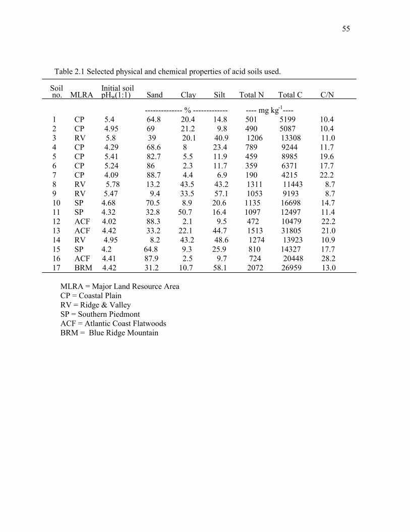
55





56

Titration curves for soil No.3 in both water and 0.01 M CaCl2

CaCO3 (kg ha-1)

0 200 400 600 800 1000 1200 1400 1600

pH

5.0

5.2

5.4

5.6

5.8

6.0

6.2

6.4

6.6

6.8

water0.01 M CaCl2


CaCO3 (kg ha-1)

0 200 400 600 800 1000 1200

pH

5.2

5.4

5.6

5.8

6.0

6.2

6.4

6.6

6.8

7.0

7.2

water0.01 M CaCl2


CaCO3 (kg ha-1)

0 500 1000 1500 2000 2500 3000 3500

pH

4.0

4.5

5.0

5.5

6.0

6.5

7.0

7.5

water0.01 M CaCl2

Titraiton curves for soil No.16 in both water and 0.01 M CaCl2

CaCO3 (kg ha-1)

0 2000 4000 6000 8000

pH

3

4

5

6

7

8

water0.01 M CaCl2


CaCO3 (kg ha-1)

0 2000 4000 6000 8000

pH

4.0

4.5

5.0

5.5

6.0

6.5

7.0

7.5

water 0.01 M CaCl2

Fig. 2.1 Titration curves for 5 soils in water and in 0.01 M CaCl2.

BM

AP ACF

RV CP

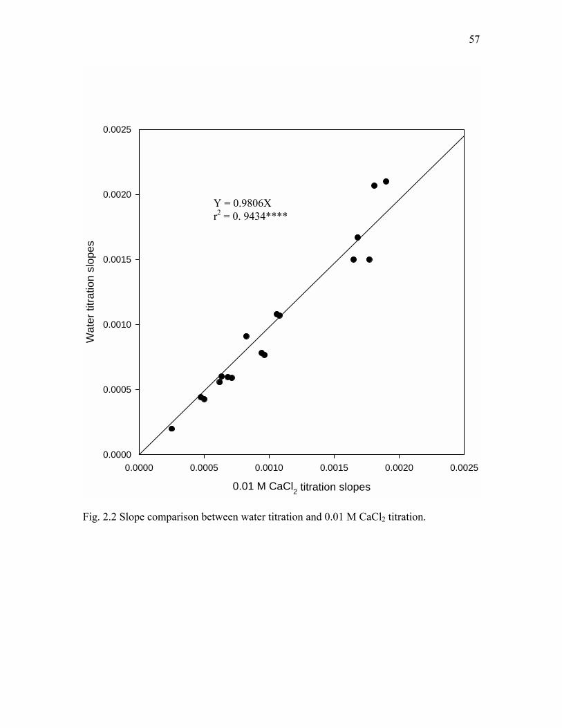
57

0.01 M CaCl2 titration slopes

0.0000 0.0005 0.0010 0.0015 0.0020 0.0025

Wat

er ti

tratio

n sl

opes

0.0000

0.0005

0.0010

0.0015

0.0020

0.0025

Fig. 2.2 Slope comparison between water titration and 0.01 M CaCl2 titration.

Y = 0.9806X r2 = 0. 9434****

58

Slopes from all data points to pH 6.5 (no first point)0.0000 0.0005 0.0010 0.0015 0.0020 0.0025

Slop

es fr

om tw

o da

ta p

oint

s (0

and

3 m

L)

0.0000

0.0005

0.0010

0.0015

0.0020

0.0025

0.0030

0.0035

Fig. 2.3 Slope comparison between data points to pH 6.5 (no first point) and two points (0 and 3 mL) in water titration.

Y = 1.3911X r2 = 0.8550****

1:1 line

59

Slopes from all data points to pH 6.50.0000 0.0005 0.0010 0.0015

Slop

es fr

om tw

o da

ta p

oint

s (0

and

3 m

L)

0.0000

0.0005

0.0010

0.0015

0.0020

0.0025

0.0030

Fig. 2.4 Comparison of titration slopes in 0.01 M CaCl2 determined by regression of all

data points vs slopes calculated from two points (0, 3 mL Ca(OH)2)

Y = 1.109X r2 = 0.8790****

1:1 line

60

LR- 3-day Ca(OH)2 incubation, kg ha-10 2000 4000 6000 8000 10000 12000 14000 16000LR

- CaC

l 2 ti

tratio

n sl

ope

(0, 3

mL)

w

ith in

itial

pH

in w

ater

, kg

ha-1

0

2000

4000

6000

8000

10000

12000

Fig. 2.5 LR comparison between readings on water titration curves and calculations

from CaCl2 titration slope (0 and 3 mL) with initial pH in water.

Y = 0.6873X r2 = 0.8983****

1:1 line

61

LR- 3-day Ca(OH)2 incubation, kg ha-10 4000 8000 12000 16000

LR- 2

poi

nt (0

and

3 m

L) p

redi

ctio

n in

0.

01 M

CaC

l 2 ti

tratio

ns, k

g ha

-1

0

4000

8000

12000

16000

Fig. 2.6 LR comparison between 2 point prediction in 0.01 M CaCl2 titrations and

3-day Ca(OH)2 incubation

Y = 0.8792X r2 = 0.9317****

: Flatwoods when those are eliminated, Y = 1.0380X r2 = 0.9272****

62

References

Alabi, K.E., R.C. Sorensen, D. Knudsen, and G.W. Rehm. 1986. Comparison of several lime requirement methods on coarse textured soils of Northeastern Nebraska. Soil Sci. Soc. Am. J. 50:937-941.

Dunn, L.E. 1943. Lime requirement determination of soils by means of titration curves. Soil Sci. 56:341-351. Follett, R.H, and R.F, Follett. 1980. Strengths and weaknesses of soil testing in determining lime requirements for soils. p 40-51. In Proc. Of the Natl. Conf. on Agric. Limestone 16-18 Oct. 1980 Magdoff, F.R. and Bartlett, R.J. 1985. Soil pH buffering revisited. Soil Sci. Soc. Am. Proc. 49:145-148. McConnell, J.S., Gilmour, J.T., Baser, R.E., and Frizzell, B.S. 1990. Lime Requirement of acid soils of Arkansas. Arkansas Experiment Station Special Report 150. Owusu-Bennoah, E., Acquaye, D. K., Mahamah, T. 1995. Comparative study of selected lime requirement methods for some acid Ghanaian soils. Commun. soil Sci. Plant Anal., 26(7&8):937-950. Ryti, R. 1965. On the determination of soil pH. Maataloustiet. Aikak. 37:51-60. Schofield, R.K., and A.W. Taylor. 1955. The measurement of soil pH. Soil Sci. Soc. Am. Proc. 19: 164-167. STATISTIX 7.0. 1985. STATISTIX for windows, 96 Analytical Software. Weaver, A.R. 2002. Characterizing soil acidity in coastal plain soils. Dissertation for pH.D. University of Georgia.

63

CHAPTER 3

CaCO3 INCUBATION METHODS REVISITED AND AN INDIRECT LIME

REQUIREMENT


Abstract

CaCO3 incubation methods are considered mostly reliable to determine the lime

requirements (LRs) of acid soils, although some studies have reported that the use of

room temperature incubation would overestimate the actual LRs determined by field

testing. One of the objectives of this study is to reveal the possible reasons for the newly

generated acidity during the incubation. Another objective is to explore the possibility of

estimating the LR from soil properties. This indirect LR estimation by soil properties is

advanced for use when the required soil properties are already known.

Seventeen soils were incubated with CaCO3 for two months at approximately 80%

field capacity under room temperature (23ûC ± 2ûC). NH+4-N and NO-

3-N were analyzed

at day 60 of the incubation. All soils were also incubated with Ca(OH)2 for 3 days. Soil

pH was lower following the 60-day CaCO3 incubation when compared to the 3-day

incubation with Ca(OH)2. The analysis of N transformations indicated that positive

values of H+ was generated after two months CaCO3 incubation in 14 cases out of 17

soils. The initial pH and total C were found to be the significant factors for the estimation

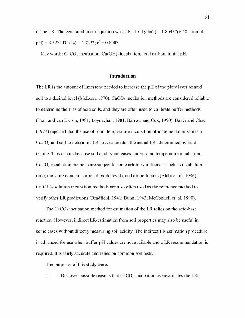
64

of the LR. The generated linear equation was: LR (103 kg ha-1) = 1.8043*(6.50 � initial

pH) + 3.5273TC (%) � 4.3292; r2 = 0.8003.

Key words: CaCO3 incubation, Ca(OH)2 incubation, total carbon, initial pH.

Introduction

The LR is the amount of limestone needed to increase the pH of the plow layer of acid

soil to a desired level (McLean, 1970). CaCO3 incubation methods are considered reliable

to determine the LRs of acid soils, and they are often used to calibrate buffer methods

(Tran and van Lierop, 1981; Loynachan, 1981; Barrow and Cox, 1990). Baker and Chae

(1977) reported that the use of room temperature incubation of incremental mixtures of

CaCO3 and soil to determine LRs overestimated the actual LRs determined by field

testing. This occurs because soil acidity increases under room temperature incubation.

CaCO3 incubation methods are subject to some arbitrary influences such as incubation

time, moisture content, carbon dioxide levels, and air pollutants (Alabi et. al. 1986).

Ca(OH)2 solution incubation methods are also often used as the reference method to

verify other LR predictions (Bradfield, 1941; Dunn, 1943; McConnell et. al, 1990).

The CaCO3 incubation method for estimation of the LR relies on the acid-base

reaction. However, indirect LR-estimation from soil properties may also be useful in

some cases without directly measuring soil acidity. The indirect LR estimation procedure

is advanced for use when buffer-pH values are not available and a LR recommendation is

required. It is fairly accurate and relies on common soil tests.

The purposes of this study were:

1. Discover possible reasons that CaCO3 incubation overestimates the LRs.

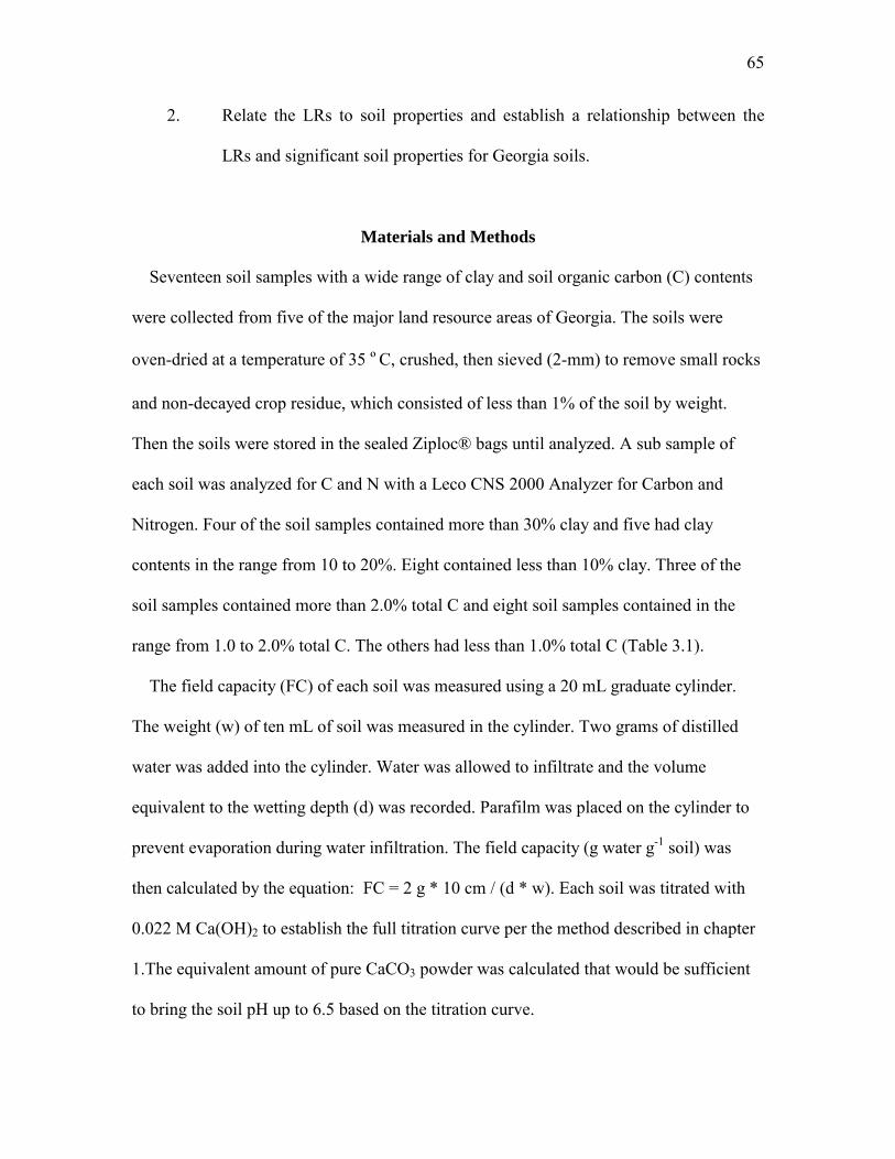
65

2. Relate the LRs to soil properties and establish a relationship between the

LRs and significant soil properties for Georgia soils.



were collected from five of the major land resource areas of Georgia. The soils were

oven-dried at a temperature of 35 ºC, crushed, then sieved (2-mm) to remove small rocks

and non-decayed crop residue, which consisted of less than 1% of the soil by weight.

Then the soils were stored in the sealed Ziploc® bags until analyzed. A sub sample of

each soil was analyzed for C and N with a Leco CNS 2000 Analyzer for Carbon and

Nitrogen. Four of the soil samples contained more than 30% clay and five had clay

contents in the range from 10 to 20%. Eight contained less than 10% clay. Three of the

soil samples contained more than 2.0% total C and eight soil samples contained in the

range from 1.0 to 2.0% total C. The others had less than 1.0% total C (Table 3.1).

The field capacity (FC) of each soil was measured using a 20 mL graduate cylinder.

The weight (w) of ten mL of soil was measured in the cylinder. Two grams of distilled

water was added into the cylinder. Water was allowed to infiltrate and the volume

equivalent to the wetting depth (d) was recorded. Parafilm was placed on the cylinder to

prevent evaporation during water infiltration. The field capacity (g water g-1 soil) was

then calculated by the equation: FC = 2 g * 10 cm / (d * w). Each soil was titrated with

0.022 M Ca(OH)2 to establish the full titration curve per the method described in chapter

1.The equivalent amount of pure CaCO3 powder was calculated that would be sufficient

to bring the soil pH up to 6.5 based on the titration curve.

66

The appropriate amount of reagent grade CaCO3 powder needed to raise the initial pH

to 6.5 was thoroughly mixed with an 80 gram sample of each soil. Treatments consisted

of the 17 soils, each receiving CaCO3 or remaining untreated. Each treatment was

replicated three times, resulting in a total of 102 samples for incubation. Enough water

was added to each soil sample to bring it to approximately 80% of field capacity. The

samples were incubated in 500 mL polyethylene containers with lids. Five-2 mm

openings were drilled through each lid for air exchange. A glass stir-rod was inserted

through one opening of each container to mix the soil. The soils were incubated for 60

days at room temperature (23ûC ± 2ûC), and were moistened every five days to keep the

water content at about 80% of field capacity. At days 30 and 60, 30 g sub samples were

taken from each container for the measurement of soil pH. The soil pH was measured at a

1:1 soil/water ratio in a 150-mL beaker.

On day 60 after the pH was measured, 120 mL of 1 M KCl was added to each soil

suspension, and transferred into a 250-mL flask. They were then stoppered and shaken at a

speed of 200 oscillation min-1 for half an hour. They were than allowed to stand for several

minutes and then filtered through a Whatman #42 filter paper. The filtrates were frozen at

-4 ûC until analyzed. Nitrate-N was analyzed with the Griess- Іlosvay technique after

reduction of NO3- to NO2

- with a Cd column (Keeney and Nelson, 1982) using an OI

Analytical Flow Solution 3000 (College Station, TX). Ammonium was analyzed using the

automated phenate colorimetric procedure EPA-600/4-79-020, �Nitrogen, Ammonia�

Method 350.1 (EPA, March 1984).


adding 30 mL of distilled water to 30 gram of each soil in a 120-mL polypropylene

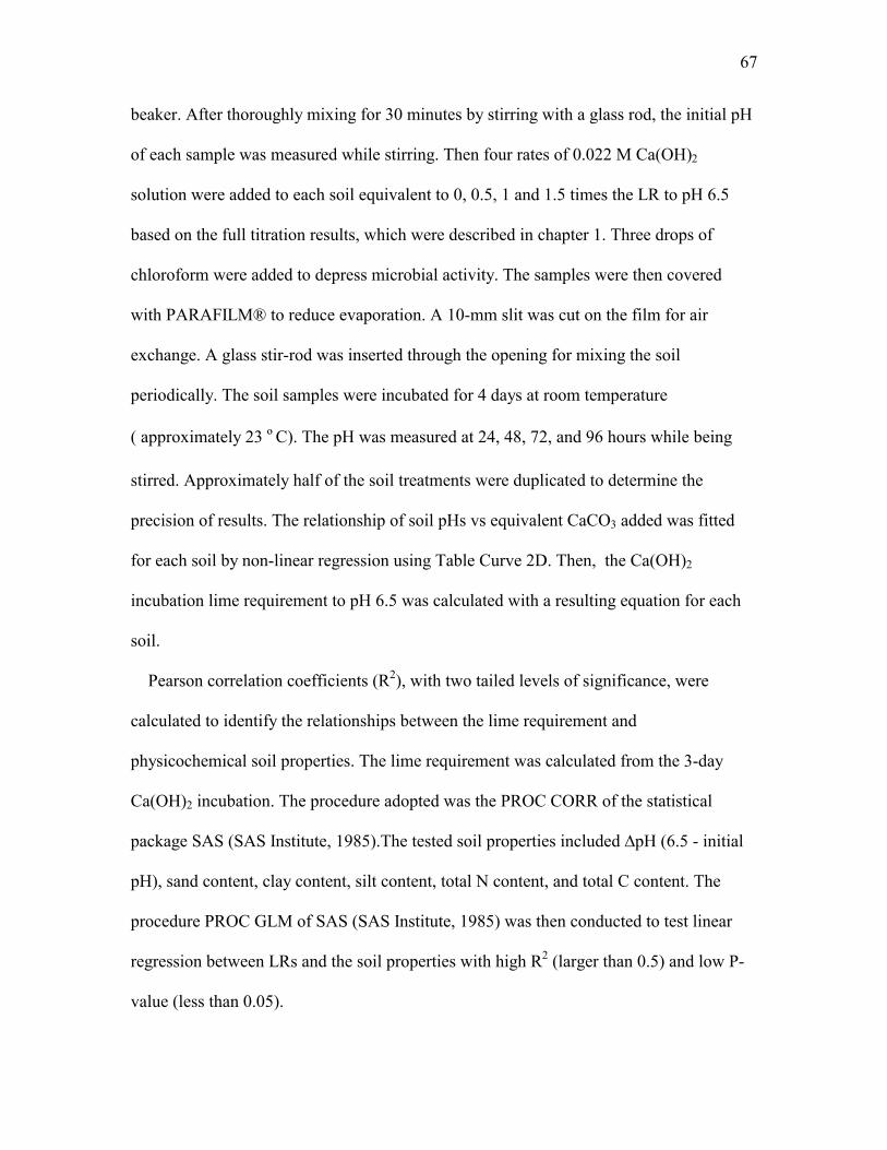
67

beaker. After thoroughly mixing for 30 minutes by stirring with a glass rod, the initial pH

of each sample was measured while stirring. Then four rates of 0.022 M Ca(OH)2

solution were added to each soil equivalent to 0, 0.5, 1 and 1.5 times the LR to pH 6.5

based on the full titration results, which were described in chapter 1. Three drops of

chloroform were added to depress microbial activity. The samples were then covered

with PARAFILM® to reduce evaporation. A 10-mm slit was cut on the film for air

exchange. A glass stir-rod was inserted through the opening for mixing the soil

periodically. The soil samples were incubated for 4 days at room temperature

( approximately 23 ºC). The pH was measured at 24, 48, 72, and 96 hours while being

stirred. Approximately half of the soil treatments were duplicated to determine the

precision of results. The relationship of soil pHs vs equivalent CaCO3 added was fitted

for each soil by non-linear regression using Table Curve 2D. Then, the Ca(OH)2

incubation lime requirement to pH 6.5 was calculated with a resulting equation for each

soil.

Pearson correlation coefficients (R2), with two tailed levels of significance, were

calculated to identify the relationships between the lime requirement and

physicochemical soil properties. The lime requirement was calculated from the 3-day

Ca(OH)2 incubation. The procedure adopted was the PROC CORR of the statistical

package SAS (SAS Institute, 1985).The tested soil properties included ∆pH (6.5 - initial

pH), sand content, clay content, silt content, total N content, and total C content. The

procedure PROC GLM of SAS (SAS Institute, 1985) was then conducted to test linear

regression between LRs and the soil properties with high R2 (larger than 0.5) and low P-

value (less than 0.05).

68


Soil pHs following the 30 and 60 day CaCO3 incubation and the 3-day Ca(OH)2

incubation are shown in table 2. If no other reactions affected the soil pH except

neutralization of the soil acidity, the soil pH value should be 6.50. In the 3-day

incubation with Ca(OH)2 the 17 soils had an average pH of 6.36 on day 3. Soil No.9

from the Ridge and Valley had the highest pH of 6.63 and soil No.13 from the

Atlantic Coast Flatwoods had the lowest value of 6.01. In the CaCO3 incubation, the

average soil pH for the 17 soils on day 30 was 5.98. Only soil No.17 from Blue Ridge

Mountains exceeded pH 6.5, with a pH of 6.60. Soil No.12 had a soil pH value 6.46.

Most of the others had values of around 6.0. The soil pH values decreased for all 17

soils on day 60 and the average value had decreased to 5.67. In the CaCO3 incubation

check soils, 13 of 17 soil pH values on day 30 had increased an average of 0.40 pH

unit from their initial pHs. This increase probably occurred because of hydrogen

consuming reactions like ammonification that dominated during the first month of

incubation, consuming hydrogen ions and raising soil pH. The check soil pH values

on day 60 dropped from the values on day 30 in almost all cases except for soil

No.17 decreasing an average of 0.21 pH unit. Seven check soils had pH values lower

than their initial pH values following 60 days of incubation.

In both incubated and check soils, the soil pH values were lower on day 60 than on day

30. This was probably due to hydrogen ion producing processes like nitrification that

dominated between 30 and 60 days of incubation. The average pH value for the 3-day

Ca(OH)2 incubation was 6.36 compared to 5.98 on day 30 of the CaCO3 incubation.

Although it appears that both CaCO3 and Ca(OH)2 incubation did not raise the soil pH to

69

the target value of 6.50, the CaCO3 incubation method may overestimate the lime

requirement of soils if we considered the 3-day Ca(OH)2 incubation as the reference

method. The N transformations during the CaCO3 incubation were positive evidence for

this conclusion (table 3.3).

The first step in the decomposition of organic N is described by the ammonification

process, which is an alkali-producing reaction:

R1-CH(NH2)-R + 1/2O2 + H2O → R1-CO-R + NH4+ +OH- (1)

where R1and R represent organic groups (Conyers et al. 1995).

Ammonium ions may be used as an energy source by the chemoautotrophic bacteria

nitrosomonas and be transformed to NO2- as shown in equation (2). Then, nitrobacter

oxides NO2- further to NO3

- as shown in equation (3) (Conyers et al. 1995).

NH4+ +3/2O2 → NO2

- + H2O +2H+ (2)

NO2- +1/2O2 → NO3

- (3)

The concentration of NH4+-N and NO3

- -N in the CaCO3 incubated soils and check soils

at day 60 are shown in table 3.3. The net H+ produced from the N transformations,

calculated using equation (1) and (2), are also listed. In the check soils, 12 of the 17 soils

gave the positive values of net H+ produced. Of the 17 CaCO3 treated soils, 14 had

positive values of H+ produced. In those cases with positive H+ values, a certain amount

of soil acidity during laboratory incubation of the soils had been generated. These results

were consistent with the conclusion of Baker and Chae (1977) for seven western

Washington soils. In cases with positive values of H+ produced, the net result will be to

lower soil pH for two reasons. First, the production of H+ in the soil will reduce pH

because the H+ will react with the pH dependent charge ( primarily soil organic matter),

70

and the corresponding drop in pH from H+ addition will also reduce soil CEC, thereby

increasing the salt content of the soil solution as some exchangeable cations are forced

into the soil solution from the reduction in CEC. The pH will be depressed further

because of the increased salt contents. The five cases of negative values of H+ in the

check soils and three in the CaCO3 incubation soils may be explained by other alkali-

producing reactions during the incubation process. According to Conyers et al. (1995)�s

study, the alkali-producing reactions may include ammonification, reduction of Mn-

oxides, oxidation of organic anions and SO4- adsorption. It was very likely that in our

study the reduction of Mn-oxides may be primarily responsible for the increase in pH

because the incubation was carried out in slightly reduced conditions since the soils were

moistened to about 80% field capacity.

The correlation coefficients (with P<0.1) are presented in Table 3.4. The lime

requirement showed significant (P < 0.05) positive linear relationships with ∆pH (6.50 �

initial pH) and total carbon content. And there was no significant relationship found

between the lime requirement and the clay content. Table 3.5 shows the GLM statistical

analysis for the linear model between the lime requirement and both ∆pH and total

carbon content. Both of the ∆pH and total carbon content were significant factors for the

lime requirements at the P level of 0.05. The GLM parameters for the linear model were

shown in Table 3.6. The linear relationship generated was:

LR (103 kg ha-1) = 1.8043*(6.50 � initial pH) + 3.5273TC (%) � 4.3292; r2 = 0.8003.

This equation can be used in the cases in which the initial pH and total carbon content

were already known.

71





72

Table 3.2 Soil pH comparison between CaCO3 incubation and Ca(OH)2 incubation.

Soil Initial soil CaCO3 incubation check Ca(OH)2 incubation no. pHw(1:1) day 30 day 60 day 30 day 60 day 3

1 5.4 6.25 6.07 5.84 5.70 6.49 2 4.95 6.02 5.91 5.49 5.32 6.46 3 5.8 5.92 5.73 5.52 5.40 6.58 4 4.29 5.37 5.02 4.71 4.52 6.32 5 5.41 6.00 5.78 5.84 5.50 6.57 6 5.24 5.80 5.56 5.22 5.06 6.34 7 4.09 5.68 5.55 4.35 4.05 6.22 8 5.78 6.00 5.85 5.52 5.40 6.59 9 5.47 5.72 5.46 5.00 4.69 6.63 10 4.68 5.70 5.30 5.29 4.50 6.21 11 4.32 6.17 5.94 4.69 4.45 6.19 12 4.02 6.46 5.79 4.33 4.32 6.32 13 4.42 5.94 5.80 4.48 4.43 6.01 14 4.95 6.01 5.41 5.11 4.96 6.44 15 4.2 6.03 5.38 4.49 4.01 6.33 16 4.41 6.07 5.53 4.91 4.82 6.10 17 4.42 6.60 6.24 5.26 5.38 6.38 Average 4.81 5.98 5.67 5.06 4.85 6.36

73

Table 3.3 Net H+ produced from N transformations in incubated soils at day 60.

Soil Original soils CaCO3 incubation check no. NO3

+-N NH4+-N NO3

+-N NH4+-N Net H+ NO3

+-N NH4+-N Net H+ µg g-1

1 7.66 4.03 15 3.97 0.5283 15.82 3.15 0.6456 2 7.29 3.53 13.46 3.15 0.4678 12.56 2.8 0.4279 3 5.87 8.5 33.82 5.74 2.1930 35.97 5.99 2.329 4 34.14 28.91 36.75 3.72 1.9853 36.87 14.55 1.2208 5 1.2 6.57 21.46 2.68 1.725 22.66 2.8 1.8018 6 9.72 3.99 21.05 1.97 0.9532 22.02 2.15 1.01 7 1.82 2.28 6.6 2.03 0.3583 5.11 2.07 0.2496 8 14.62 4.92 29.25 3.25 1.1639 29.31 2.59 1.2153 9 1.82 5.04 18.87 2.58 1.3933 20.01 2.35 1.4917 10 8.28 8.59 29.99 2.34 1.9969 30.43 3.98 1.9115 11 2.56 7.97 14.88 27.21 -0.4938 14.86 6.79 0.9626 12 1.03 6.76 19.47 2.66 1.6099 1.53 25.38 -1.2943 13 1.86 9.4 1.71 51.85 -3.0434 1.26 46.36 -2.6834 14 1.59 12.99 30.1 9.97 2.2523 7.05 52.1 -2.4057 15 5.46 7.45 34.36 2.43 2.4222 23.25 2.54 1.6208 16 1.57 7.16 18.38 2.67 1.5217 2.94 28.35 -1.4159 17 2.03 19 19.39 101.1 -4.6239 1.46 138.4 -8.5692

H+ (mol) produced from nitrification = 2*(NO3

+-Nincubation - NO3+-Noriginal) (mol)

H+ (mol) consumed from ammonification = (NO3

+-N + NH4+-N)incubation (mol)

- (NO3+-N + NH4

+-N)original (mol) Net H+ (mol) = H+ (mol) produced - H+ (mol) consumed Net H+ (µg g-1) = Net H+ (mol) * 1 g mol-1 g-1 soil

74

Table 3.4 Pearson correlation coefficients among physicochemical properties of 17 soils and lime requirements (LR). Soil property ∆pH sand clay silt TN TC LR 0.526** --- --- --- 0.471* 0.845****

two tailed levels of significance: --- P ≥ 0.1; * P < 0.1; ** P < 0.05; *** P < 0.001; **** P < 0.0001 ∆pH = 6.5 - initial pH; TN = total N; TC = total Carbon; LR = lime requirement

75

Table 3.5 GLM Table for the linear model of lime requirement (103 kg ha-1) relating to ∆pH and total carbon content (%). Source df Type ІІІ SS MS F Pr > F ∆pH 1 17.289 17.289 6.06 0.0274

TC 1 104.752 104.752 36.73 < .0001

Error 14 39.929 2.852

Total 16 161.97

∆pH = 6.50 � initial pH; TC = total carbon content

76

Table 3.6 GLM Parameter table for the linear model of lime requirement (103 kg ha-1)

relating to ∆pH and total carbon content (%).

Parameter Estimate Standard Error t value Pr > | t |

Intercept -4.3292 1.3127 -3.30 0.0053

∆pH 1.8043 0.7328 2.46 0.0274

TC 3.5273 0.5820 6.06 < .0001

∆pH = 6.50 � initial pH; TC = total carbon content

77

References

Alabi, K.E., R.C. Sorensen, D. Knudsen, and G.W. Rehm. 1986. Comparison of several lime requirement methods on coarse textured soils of Northeastern Nebraska. Soil Sci. Soc. Am. J. 50:937-941. Backer, A.S., and Y.M. Chae. 1977. A laboratory quick test for predicting the lime requirements of acid mineral soils. Tech. Bull. 88, Washington State Univ., 11 p. Barrow, N.J, and Cox, V.C. 1990. A quick and simple method for determining the titration curve and estimating the lime requirement of soils. Austra. J. Soil Research: 28:685-694. Bradfield, R. 1941. Calcium in the soil: 1. Physico-chemical relations. Soil Sci. Soc. Am. Proc.6:8-15. Conyers, M. K., N. C. Uren and K. R. Helyar. 1995. Causes of changes in pH in acidic mineral soils. Soil Biol. Biochem. 27:1383-1392. Dunn, L.E. 1943. Lime requirement determination of soils by means of titration curves. Soil Sci. 56:341-351.

EPA. March, 1984. Methods for chemical analysis of water and wastes. EPA-600/4-79-020.

�Nitrogen, Ammonia� Methid 350.1 (Colorimetric, Automated Phenate) Storet No. Total 00610,

Dissolved 00608.

Keeney, D.R., and D.W. Nelson. 1982. Nitrogen-Inorganic forms. p. 634-698. In A.L. Page et al.

(ed.) Methods of soil analysis. Part 2. Chemical and microbiological properties. 2nd ed. Agron.

Monogr.9. ASA and SSSA, Madison, WI.

Loynachan, T.E. 1981. Lime requirement methods for cold regions. Soil Sci. Soc. Am. J. 45:77-80.

McConnell, J.S., Gilmour, J.T., Baser, R.E., and Frizzell, B.S. 1990. Lime Requirement of acid soils of Arkansas. Arkansas Experiment Station Special Report 150.

McLean, E.O. 1970. Lime requirement of soils-inactive toxic substances or favorable pH range.

Soil Sci. Soc. Am. Proc. 34:363-364.

78

SAS Institute. 1985. SAS user�s guide: Statistics. Version 6 ed. SAS Institute, Inc., Carg, NC.

Tran, T. S., and W. van Lierop. 1981. Evaluation and improvement of buffer-pH lime requirement methods. Soil Sci. 131:178-188.

79

APPENDIX Fig. 1 Titration curves for twelve soils in water and 0.01 M CaCl2.


CaCO3 (kg ha-1)

0 200 400 600 800 1000 1200 1400

pH

5.0

5.5

6.0

6.5

7.0

7.5

water0.01 M CaCl2


CaCO3 (kg ha-1)

0 200 400 600 800 1000 1200

pH

4.8

5.0

5.2

5.4

5.6

5.8

6.0

6.2

6.4

6.6

6.8

water0.01 M CaCl2


CaCO3 (kg ha-1)

0 500 1000 1500 2000 2500 3000

pH

4.0

4.5

5.0

5.5

6.0

6.5

7.0

7.5

water0.01 M CaCl2


CaCO3 (kg ha-1)0 200 400 600 800 1000 1200 1400 1600

pH

4.5

5.0

5.5

6.0

6.5

7.0

7.5

water0.01 M CaCl2

80


CaCO3 (kg ha-1)

0 500 1000 1500 2000 2500

pH

3.5

4.0

4.5

5.0

5.5

6.0

6.5

7.0

7.5

water0.01 M CaCl2


CaCO3 (kg ha-1)

0 500 1000 1500 2000 2500 3000 3500

pH

5.0

5.2

5.4

5.6

5.8

6.0

6.2

6.4

6.6

6.8

7.0

7.2

water0.01 M CaCl2


CaCO3 (kg ha-1)0 500 1000 1500 2000 2500 3000 3500

pH

4.5

5.0

5.5

6.0

6.5

7.0

7.5

water0.01 M CaCl2


CaCO3 (kg ha-1)0 1000 2000 3000 4000 5000 6000

pH

3.5

4.0

4.5

5.0

5.5

6.0

6.5

7.0

7.5

water0.01 M CaCl2

81


CaCO3 (kg ha-1)

0 1000 2000 3000 4000 5000 6000

pH

3

4

5

6

7

8

water0.01 M CaCl2


CaCO3 (kg ha-1)

0 2000 4000 6000 8000 10000 12000 14000

pH

3.5

4.0

4.5

5.0

5.5

6.0

6.5

7.0

water0.01 M CaCl2


CaCO3 (kg ha-1)

0 1000 2000 3000 4000 5000 6000

pH

4.0

4.5

5.0

5.5

6.0

6.5

7.0

7.5

water0.01 M CaCl2


CaCO3 (kg ha-1)

0 1000 2000 3000 4000 5000

pH

3.5

4.0

4.5

5.0

5.5

6.0

6.5

7.0

7.5

water0.01 M CaCl2

direct titration for measurement of soil … titration for measurement of soil lime requirement and...

Documents