Development of soil pH and lime requirement maps using on-the-go soil sensors

E.D. Lund1, V.I. Adamchuk

2, K.L. Collings

1, P.E. Drummond

1 and C.D. Christy

1

1 Veris Technologies, Inc., 601 N. Broadway, Salina, KS 67401, USA 2 University of Nebraska-Lincoln, Lincoln, NE 68583-0726, USA

lunde@veristech.com

Abstract

Since conventional sampling and laboratory soil analysis do not provide a cost effective

capability to obtain georeferenced measurements with adequate frequency, different on-

the-go sensing techniques have been attempted. One such recently commercialized

sensing system combines mapping of soil electrical conductivity and pH. The concept

of direct measurement of soil pH has allowed for a substantial increase in measurement

density. In this publication, the analysis of variable rate lime prescription maps is

discussed. Liming rates generated from on-the-go measurements can result in improved

prediction of liming requirement compared to the conventional 1 ha grid sampling

(RMSE = 1354 versus 2506 kg/ha).

Keywords: on-the-go mapping, soil pH; variable rate liming; electrical conductivity.

Introduction

Site-specific crop management allows growers to improve management of agricultural

inputs while taking into consideration the variability of soil attributes within their fields.

Conventional geo-referenced soil sampling and laboratory analysis represent a popular

technique to identify the variability of soil properties within fields (Whipker and

Akridge, 2004). Sampling fields using a 1 ha grid pattern has become the most common

strategy in many parts of the USA. To define soil test values for locations between the

sampling points, various interpolation methods have been used. The interpolated values

predicted for un-sampled areas are valid only if there is spatial dependence between the

sample sites. Interpolation of a map based on unrelated soil test values is erroneous.

Several studies have shown that the range of soil pH spatial dependency can be less than

100 m, the length of a 1 ha grid cell (McBratney and Pringle, 1997). For example, in

some cases, semivariogram ranges (maximum distances of spatial dependency) as short

as 21 m have been found (Wollenhaupt et al., 1997) while, in some fields, changes of 2

pH units have been observed over distances less than 12 m (Bianchini and Mallarino,

2002). Higher sampling density has been shown to be impractical because of the high

sampling and analysis costs. Attempts have been made to improve spatial predictions

from soil sampling using more rigorous geostatistical methods (McBratney et al., 1981;

Laslett and McBratney, 1990). These approaches required sampling densities higher

than the common 1 ha intensity and, therefore, have not been adopted commercially.

As an alternative, on-the-go soil sensors offer the potential to increase mapping density

at a relatively low cost (Viscarra Rossel and McBratney, 1997). Based on the experience

gained during the development of a field prototype system for mapping soil nitrate

content and pH (Loreto and Morgan, 1996), a research study was initiated in 1997 to

investigate the applicability of flat-surface combination ion-selective electrodes (ISEs)

to measure soil properties (particularly pH) on moist soil samples directly (Adamchuk et

al., 2003). The initial results illustrated high correlation with conventional laboratory

measurements (r² > 0.92), and a prototype automated system for mapping soil pH on-

the-go was developed and tested (Adamchuk et al., 1999). Later, this technology was

licensed (Veris Technologies, Inc., Salina, Kansas, USA), and a commercial implement

(Soil pH Manager™) has been developed (www.veristech.com). While most operation

parameters are selected by users, this sensor can be operated at 8 km/hr using 20 m

transects (distance between passes) while conducting measurements every 10 s, which

results in more than 20 measurements obtained from each hectare.

Although more accurate delineation of field areas requiring lime application was

achieved, it was also known that lime requirements depend not only on soil pH, but also

on soil buffering characteristics commonly assessed through buffer pH test or direct

titration methods. Conventional apparent electrical conductivity (EC) maps have been

shown to correspond to changes in soil types and therefore related to buffering

characteristics (McBride et al., 1990). Therefore, the Soil pH ManagerTM was integrated

with the Veris® 3100 EC mapping unit to form the Veris

® Mobile Sensor Platform

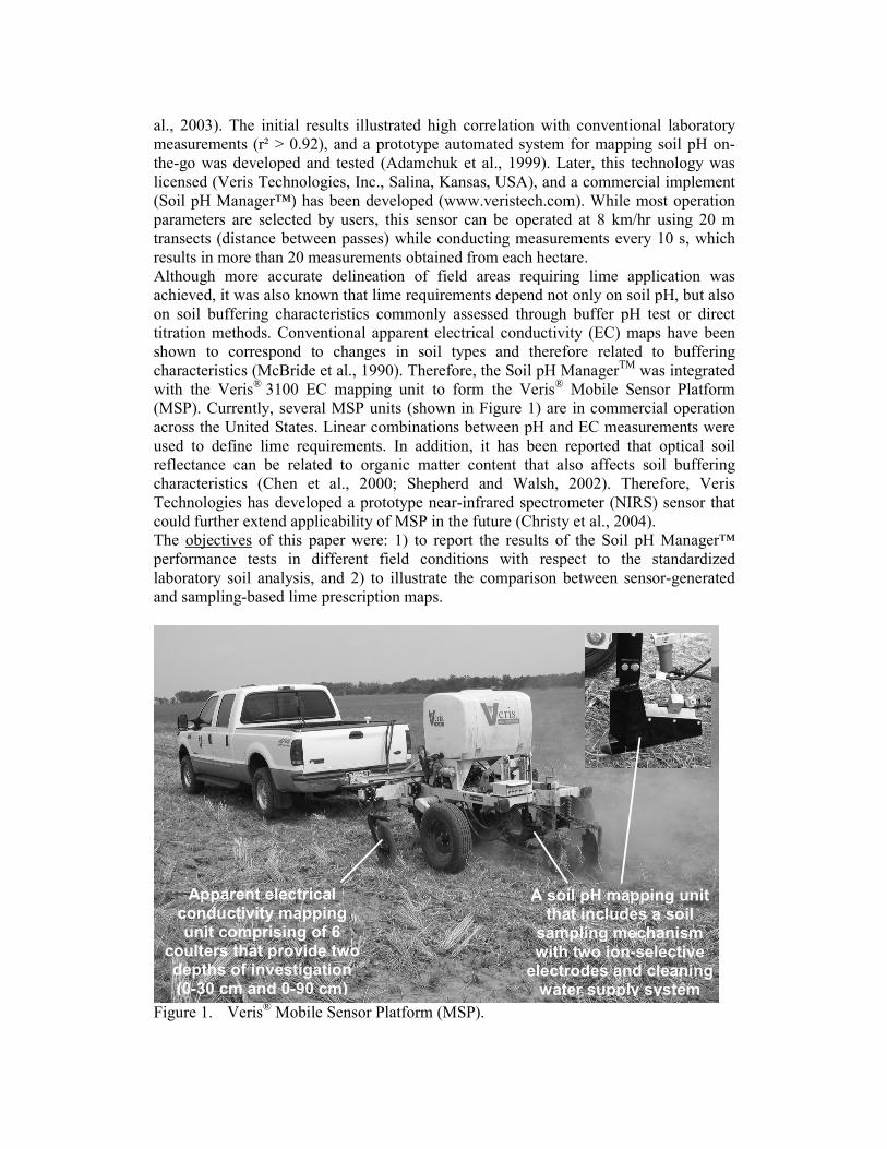
(MSP). Currently, several MSP units (shown in Figure 1) are in commercial operation

across the United States. Linear combinations between pH and EC measurements were

used to define lime requirements. In addition, it has been reported that optical soil

reflectance can be related to organic matter content that also affects soil buffering

characteristics (Chen et al., 2000; Shepherd and Walsh, 2002). Therefore, Veris

Technologies has developed a prototype near-infrared spectrometer (NIRS) sensor that

could further extend applicability of MSP in the future (Christy et al., 2004).

The objectives of this paper were: 1) to report the results of the Soil pH Manager™

performance tests in different field conditions with respect to the standardized

laboratory soil analysis, and 2) to illustrate the comparison between sensor-generated

and sampling-based lime prescription maps.

Figure 1. Veris

® Mobile Sensor Platform (MSP).

Apparent electrical conductivity mapping unit comprising of 6

coulters that provide two depths of investigation (0-30 cm and 0-90 cm)

A soil pH mapping unit that includes a soil

sampling mechanism with two ion-selective electrodes and cleaning water supply system

Materials and methods

Automated mapping of soil pH

During field operation, the Soil pH ManagerTM automatically collects and measures a

soil sample without stopping and without any action from the operator. Measurement

depth is adjustable from 4 to 15 cm. The direct soil measurements performed on-the-go

are conducted by two combination, jell-filled, epoxy-body, dome-glass membrane, ion-

selective pH electrodes. Soil cores are brought into direct contact with the electrodes

and held in place for 7- 25 s (depending on the electrode response). Average cycle time

is approximately 10 seconds. Every measurement represents an average of the outputs

produced by two electrodes. This is done to cross-validate electrode performance and

filter erroneous readings.

While mapping a field, optional row cleaners remove crop residue. A hydraulic cylinder

on a parallel linkage retracts to lower the cutting shoe assembly into the soil thus cutting

a soil core which flows into a sampling trough. The previous core sample is discharged

out of the rear of the trough by the new sample core entering in the front. The hydraulic

cylinder extends to raise the sampling trough containing the soil core out of the soil

while bringing the new soil core into contact with two ion-selective pH electrodes in an

electrode holder. During each raising and lowering cycle, the leading edge of the cutting

shoe is cleaned by the cutting shoe scraper. The electrodes are washed with two flat fan

nozzles while sampling a new core; water is held in a 378 L tank. Optional covering

disks fill the soil trench and cover the track. An external electronic control module

operates the sampling process, records the output of the ion-selective electrodes and

sends these readings to a data storage and user interface module. The instrument

processes electrode voltage output and converts it to pH. A two point calibration

procedure is performed using standard buffer solutions corresponding to pH 4, 7, and

(for alkaline soils) 10. Every measurement is georeferenced using a Global Positioning

System (GPS) receiver.

Field evaluation

A pre-commercial prototype of Soil pH ManagerTM was tested on more than 1200 ha

across nine US states. Every field was mapped using transect widths of approximately

15-20 m, and field speeds ranging from 8 to 16 km/hr. This resulted in mapping density

varying between 10 and 20 samples/ha. More than 15,000 measurements with two

electrodes have been obtained. To validate the sensor measurements, 329 manually

extracted soil samples were collected and analyzed in a commercial laboratory (Soil

Testing Lab, Kansas State University, Manhattan, Kansas, USA) following the standard

analytical procedure (Watson and Brown, 1998).

Sample locations were determined based on 0.4 ha or 1 ha systematic aligned grids,

and/or adaptive sampling to target the areas of apparent homogeneity (based on EC and

pH maps). At each of the sampling points, 8-10 soil cores were collected from a depth

of 0-15 cm within a circle with 3 m radius. These cores were mixed prior to submitting

to the laboratory. The results of the laboratory analysis were compared to the inverse-

distance weighted average of two nearest on-the-go measurements performed within

7 m from the center of the manual soil sample location (a single on-the-go measurement

was used when a second nearest measurement was farther then 7 m from the sampling

location). On-the-go sensor measurements were normalized to the field means of the

laboratory results.

The coefficient of determination of linear regression between corresponding laboratory

and on-the-go measurement of soil pH was the major indicator of overall field

performance of the on-the-go soil pH mapping. Root mean squared error (RMSE)

calculated as the root of squared difference between two corresponding measurements

was used to quantify sensor’s performance in individual fields. In this case the

assumption of 1:1 relationship between two measurement methods was applied.

Lime requirement

In addition to on-the-go soil pH mapping, several fields were mapped using EC sensors

and one field was mapped with pH, EC, and NIRS sensors. The EC measurements were

obtained using traditional Veris® 3100 unit (Lund et al., 1998). Soil optical reflectance

was determined using a newly designed shank-based NIRS system (Christy et al.,

2004). This instrument recorded soil reflectance between 900 and 1700 nm.

Calcium and/or magnesium soil amendments (such as lime) are typically applied to

neutralize acidic soil (low soil pH). In many regions, the quantity of required lime is

found through an additional pH measurement of a buffer (typically SMP or Woodruff)

extract. The lime requirement is affected by several factors: weathering, type of parent

material, clay content, organic matter content, forms of acidity present, as well as the

initial and the final soil pH (McLean and Brown, 1984). With crude approximation, soil

buffering characteristic can be predicted based on soil texture. For example, Hoeft et al.

(1996) recommend Illinois producers to apply lime recommendations based on soil pH

and generic soil characteristics affected by primarily soil texture. Bulk soil electrical

conductivity (EC) measured on-the-go has frequently been used as an indirect indicator

of soil texture (Sudduth, et al., 2002). Soil optical reflectance usually correlates with

organic matter (Chen, et al., 2000) can be associated with soil buffering as well.

Therefore, integrating soil EC and optical reflectance mapping capability can potentially

improve applicability of on-the-go soil pH mapping to derive lime prescription maps.

To evaluate the potential of on-the-go soil mapping for variable rate liming, four fields

were mapped using the on-the-go soil sensors and sampled manually on a 1 ha grid.

Manual samples were analyzed for soil pH as well as buffer pH (based on the

conventional SMP buffer test). The buffer pH test results were used to define lime

requirement based on existing Kansas State University (Manhattan, Kansas, USA) soil

fertility recommendations. The following three major liming strategies have been

compared: 1) uniform lime application rate based on the average of buffer pH

measurements, 2) variable rate liming based on conventional 1 ha grid soil sampling

results processed using the inverse-distance second-power interpolation, and 3) variable

rate liming based on on-the-go soil sensors data. Lime prescription maps based on on-

the-go mapping were developed using three levels of data: 1) soil pH maps only, 2) soil

pH and EC maps, and 3) soil pH, EC and NIRS data combined. Simple linear regression

was used to define buffer pH (and therefore lime requirement) as a function of soil pH

or linear combination of soil pH and shallow (0-30 cm) EC measurements. A locally-

weighted partial least squares regression analysis was used to predict buffer pH when

NIRS sensor data was involved. The combination of all three data layers to predict

buffer pH was available for only one production field.

Ten directed soil samples were used to determine the relationship between buffer pH

measured in the laboratory and sensor outputs. Samples obtained using a 1 ha grid

pattern were used to validate lime requirement maps based on sensor data. On the other

hand, the directed soil samples were used to validate conventional liming strategies

(uniform management and variable rate liming based on manually collected grid

sampling). The RMSE (root MSE) was calculated for each field and served as the major

indicator of map quality. The MSE (mean squared error), which served as a variance of

error estimate used to make statistical comparison (F-test), was defined as the averaged

squared difference between lime requirements (based on laboratory buffer pH

measurements) at validation points and corresponding values from lime prescription

maps.

Results and Discussion

Soil pH measurements

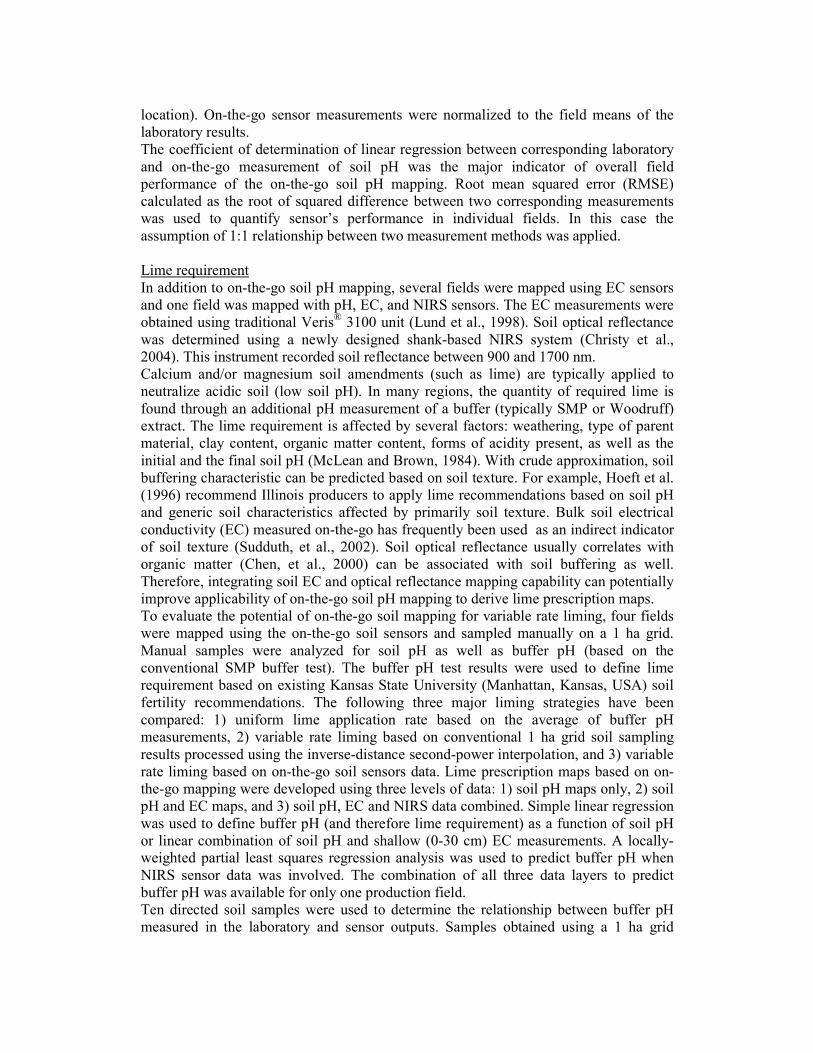
The results of the comparison between soil pH measurements performed in the

laboratory and in the field are summarized in Table 1. Although some fields

demonstrated a lower degree of correlation between corresponding on-the-go and

laboratory measurements, coefficient of determination values (r2) greater than 0.4 have

been observed in every field. Differences between the two measurement methods may

be explained by on-the-go measurements and soil samples being up to 7 m apart, and by

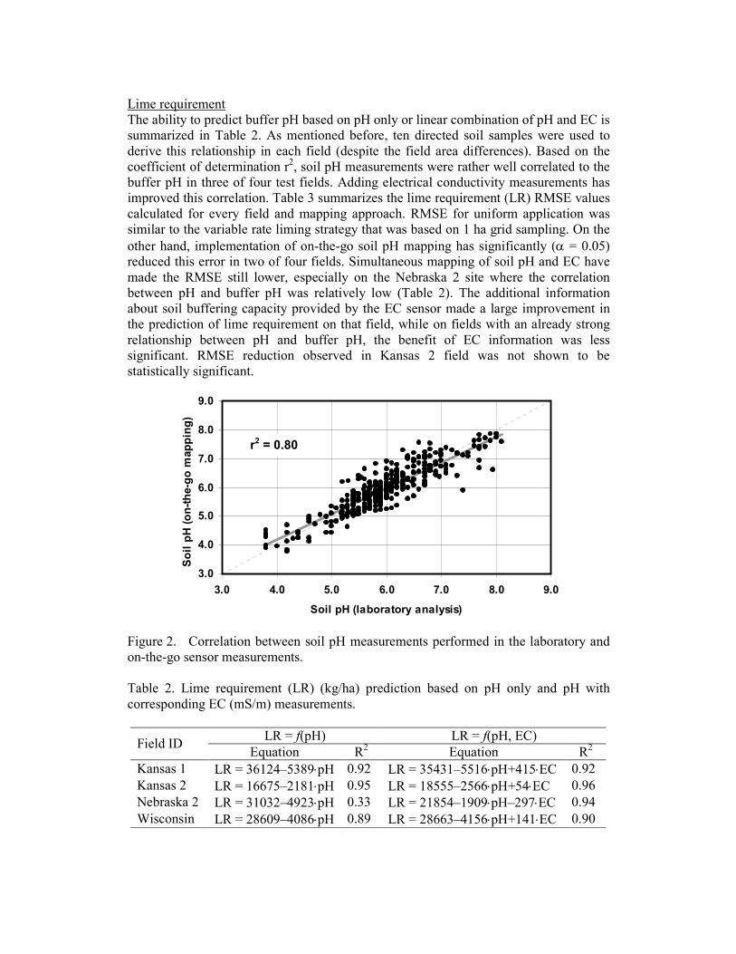
being from different depths. . The overall comparison (Figure 2) indicated relatively

high correlation (r2 = 0.80) with the slope of linear regression being close to one. The

overall RMSE was found to be 0.38 and ranged from 0.28 to 0.55 pH for different

fields.

Table 1. Summary of soil pH measurement comparison in 14 production fields.

Number of measurements Field ID Area, ha

On-the-go Manual r2*

RMSE*,

pH

Illinois 1 30 260 10 0.76 0.30

Illinois 2 22 184 10 0.65 0.51

Illinois 3 30 272 10 0.85 0.36

Iowa 12 107 37 0.76 0.39

Kansas 1 20 598 34 0.76 0.34

Kansas 2 15 706 67 0.63 0.39

Kansas 3 32 456 10 0.86 0.33

Kansas 4 47 791 10 0.74 0.30

Kansas 5 32 333 15 0.78 0.28

Kansas 6 25 250 15 0.77 0.33

Kansas 7 10 199 26 0.77 0.39

Nebraska 1 30 286 42 0.40 0.41

Nebraska 2 11 250 22 0.42 0.55

Wisconsin 13 260 24 0.71 0.55

Overall 329 4952 332 0.80 0.38 *coefficient of determination and RMSE values were determined using linear

regression model: Sensor pH = β0 + β1⋅ Lab pH

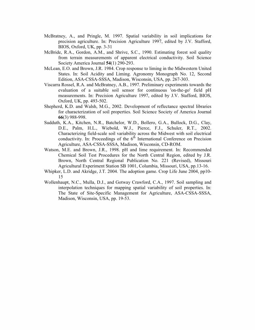
Lime requirement

The ability to predict buffer pH based on pH only or linear combination of pH and EC is

summarized in Table 2. As mentioned before, ten directed soil samples were used to

derive this relationship in each field (despite the field area differences). Based on the

coefficient of determination r2, soil pH measurements were rather well correlated to the

buffer pH in three of four test fields. Adding electrical conductivity measurements has

improved this correlation. Table 3 summarizes the lime requirement (LR) RMSE values

calculated for every field and mapping approach. RMSE for uniform application was

similar to the variable rate liming strategy that was based on 1 ha grid sampling. On the

other hand, implementation of on-the-go soil pH mapping has significantly (α = 0.05)

reduced this error in two of four fields. Simultaneous mapping of soil pH and EC have

made the RMSE still lower, especially on the Nebraska 2 site where the correlation

between pH and buffer pH was relatively low (Table 2). The additional information

about soil buffering capacity provided by the EC sensor made a large improvement in

the prediction of lime requirement on that field, while on fields with an already strong

relationship between pH and buffer pH, the benefit of EC information was less

significant. RMSE reduction observed in Kansas 2 field was not shown to be

statistically significant.

3.0

4.0

5.0

6.0

7.0

8.0

9.0

3.0 4.0 5.0 6.0 7.0 8.0 9.0

Soil pH (laboratory analysis)

Soil pH (on-the-go m

apping)

Figure 2. Correlation between soil pH measurements performed in the laboratory and

on-the-go sensor measurements.

Table 2. Lime requirement (LR) (kg/ha) prediction based on pH only and pH with

corresponding EC (mS/m) measurements.

LR = f(pH) LR = f(pH, EC) Field ID

Equation R2 Equation R

2

Kansas 1 LR = 36124–5389⋅pH 0.92 LR = 35431–5516⋅pH+415⋅EC 0.92

Kansas 2 LR = 16675–2181⋅pH 0.95 LR = 18555–2566⋅pH+54⋅EC 0.96

Nebraska 2 LR = 31032–4923⋅pH 0.33 LR = 21854–1909⋅pH–297⋅EC 0.94

Wisconsin LR = 28609–4086⋅pH 0.89 LR = 28663–4156⋅pH+141⋅EC 0.90

r2 = 0.80

Table 3. Comparison of three liming strategies based on data obtained conventionally or

using the on-the-go soil sensors.

Root mean squared error (RMSE)**, kg/ha

On-the-go mapping Field ID

Number of

validation

samples* Uniform

liming

Grid

sampling pH only pH and EC

Kansas 1 10 / 32 3550 3085 1117UG 797

UGP

Kansas 2 10 / 57 1930 1745 1470 1450

Nebraska 2 10 / 12 2527 2088 2701 1120 UGP

Wisconsin 10 / 14 2900 2781 1400 UG 1444

UG

Overall 40 / 89 2857 2506 1354 UG 1259

UG

* – Ten targeted samples were used to validate uniform liming and grid sampling

approaches in every field and grid samples were used to validate on-the-go mapping ** – RMSE values are shown for reference only, all comparisons were done using F-

statistic performed on the estimates of error variance (MSE) U – significant (α = 0.05) decrease of MSE compared to the uniform liming G – significant (α = 0.05) decrease of MSE compared to the grid sampling P – significant (α = 0.05) decrease of MSE compared to the on-the-go mapping of pH

only

One of these fields (Kansas 1) was mapped using the NIRS sensor in addition to the pH

and EC maps. Lime requirement maps generated based on the three sensors have further

reduced RMSE (643 kg/ha) versus 1117 (significant at α = 0.05) and 797 (insignificant

at α = 0.05) kg/ha when lime requirement maps were based on pH only and on the

combination of pH and EC maps, respectively. Lime requirements determined using

sensor data and in the laboratory are compared in Figure 3. In this field, the correlation

between corresponding lime requirement estimates also increased when multiple on-the-

go soil sensing techniques were used.

Figure 3. Comparison of lime requirement determined using buffer pH laboratory

measurements and on-the-go soil sensors (a – pH only, b – pH, EC and

NIRS) in a production field (Kansas 1).

r2 = 0.83

2000

4000

6000

8000

10000

2000 4000 6000 8000 10000

Measured lime requirement, kg/ha

Predicted lim

e requirement,

kg/ha

r2 = 0.52

2000

4000

6000

8000

10000

2000 4000 6000 8000 10000

Measured lime requirement, kg/ha

Predicted lim

e requirement,

kg/ha

Prediction is based on pH map only Prediction is based on pH, EC, and NIRS maps

a) b)

Conclusions

Automated mapping of soil pH on-the-go has become available commercially. It has

been found that the Soil pH ManagerTM could produce 20 times more measurements

than 1 ha grid sampling with a comparable effort. Validation sampling of sensor

measurements resulted in acceptable correlation with conventional laboratory analyses.

In addition, sensor-based lime prescription maps showed a reduced error in lime

application rates. In selected fields, this improvement can be enhanced through

incorporation of additional on-the-go soil sensors: conventional electrical conductivity

sensor (commercial) and near-infrared spectroscopy (NIRS) sensors (under

development).

References

Adamchuk, V.I., Morgan, M.T. and Ess, D.R., 1999. An automated sampling system for

measuring soil pH. Transactions of the ASAE 42(4) 885-891.

Adamchuk, V.I., Lund, E.D., Dobermann, A., and Morgan, M.T., 2003. On-the-go

mapping of soil properties using ion-selective electrodes. In: Proceedings of the

4th European Conference on Precision Agriculture, J. Stafford and A. Werner,

eds. Wageningen Academic Publishers, Wageningen, The Netherlands, pp.

27-33.

Bianchini, A.A. and Mallarino, A.P., 2002. Soil-sampling alternatives and variable-rate

liming for a soybean-corn rotation. Agronomy Journal 94(6) 1355-1366.

Chen, F., Kissel, D.E., West, L.T., and Adkins, W., 2000. Field-scale mapping of

surface soil organic carbon using remotely sensed imagery. Soil Science Society

of America Journal 64(2) 746-753.

Christy, C.D.Drummond, P.E., Laird, D.A., 2003. An on-the-go spectral reflectance

sensor for soil. Paper No. 031044. ASAE, St. Joseph, Michigan, USA.

Christy, C., Collings, K.L.,Drummond, P.D., and Lund, E.D., 2004. A mobile sensor

platform for measurement of soil pH and buffering. Paper No. 041042. ASAE,

St. Joseph, Michigan, USA.

Hoeft, R.G., Peck, T.R., and Boone, L.V., 1996. Soil testing and fertility. In: Illinois

Agronomy Handbook 1995-1996. Circular 1333, Cooperative Extension

Service, College of Agriculture, University of Illinois, Urbana, Illinois, USA,

pp. 70-101.

Laslett, G.M. and McBratney, A.B., 1990. Further comparison of spatial methods for

predicting soil pH. Soil Science Society of America Journal Vol 54 No. 6

pp.1553-1558.

Loreto, A.B. and Morgan, M.T. 1996. Development of an automated system for field

measurement of soil nitrate. Paper No. 961087, ASAE, St. Joseph, Michigan,

USA.

Lund, E.D., Christy, C.D., and Drummond, P.E., 1998. Applying soil electrical

conductivity technology to precision agriculture. In: Proceedings of the 4th

International Conference on Precision Agriculture, ASA-CSSA-SSSA, Madison,

Wisconsin, USA, pp. 1089-1100.

McBratney, A.B., Webster, R., and Burgess, T.M., 1981. The design of optimal

sampling schemes for local estimation and mapping of regionalized variables-1.

Computers and Geosciences 7(4) 331-334.

McBratney, A., and Pringle, M. 1997. Spatial variability in soil implications for

precision agriculture. In: Precision Agriculture 1997, edited by J.V. Stafford,

BIOS, Oxford, UK, pp. 3-31

McBride, R.A., Gordon, A.M., and Shrive, S.C., 1990. Estimating forest soil quality

from terrain measurements of apparent electrical conductivity. Soil Science

Society America Journal 54(1) 290-293.

McLean, E.O. and Brown, J.R. 1984. Crop response to liming in the Midwestern United

States. In: Soil Acidity and Liming. Agronomy Monograph No. 12, Second

Edition, ASA-CSSA-SSSA, Madison, Wisconsin, USA, pp. 267-303.

Viscarra Rossel, R.A. and McBratney, A.B., 1997. Preliminary experiments towards the

evaluation of a suitable soil sensor for continuous 'on-the-go' field pH

measurements. In: Precision Agriculture 1997, edited by J.V. Stafford, BIOS,

Oxford, UK, pp. 493-502.

Shepherd, K.D. and Walsh, M.G., 2002. Development of reflectance spectral libraries

for characterization of soil properties. Soil Science Society of America Journal

66(3) 988-998.

Sudduth, K.A., Kitchen, N.R., Batchelor, W.D., Bollero, G.A., Bullock, D.G., Clay,

D.E., Palm, H.L., Wiebold, W.J., Pierce, F.J., Schuler, R.T., 2002.

Characterizing field-scale soil variability across the Midwest with soil electrical

conductivity. In: Proceedings of the 6th International Conference on Precision

Agriculture, ASA-CSSA-SSSA, Madison, Wisconsin, CD-ROM.

Watson, M.E. and Brown, J.R., 1998. pH and lime requirement. In: Recommended

Chemical Soil Test Procedures for the North Central Region, edited by J.R.

Brown, North Central Regional Publication No. 221 (Revised), Missouri

Agricultural Experiment Station SB 1001, Columbia, Missouri, USA, pp.13-16.

Whipker, L.D. and Akridge, J.T. 2004. The adoption game. Crop Life June 2004, pp10-

15

Wollenhaupt, N.C., Mulla, D.J., and Gotway Crawford, C.A., 1997. Soil sampling and

interpolation techniques for mapping spatial variability of soil properties. In:

The State of Site-Specific Management for Agriculture, ASA-CSSA-SSSA,

Madison, Wisconsin, USA, pp. 19-53.