diﬀraction stack migration 2 diﬀraction stack migration the basic assumption in resorting shot...

Chapter 2

Diffraction Stack Migration

The basic assumption in resorting shot gathers into common midpoint gathers, applyingNMO corrections, and stacking is that the reflectors are flat with no lateral velocity changes.If true, the origin of the stacked reflection energy originates somewhere directly beneaththe trace, as shown in Figure 2.1. However, this will not be true for strong lateral velocityvariations or layering that departs from the horizontal, such as the dipping layers shown inFigures 1.8, 2.2, 1.11, and 2.2, with the consequence that the reflection energy could haveoriginated at a depth horizontally offset from the trace position. Thus we need to ”migrate”the reflection to its point or origin, a process commonly known as migration. Not doing sowill lead to mispositioning errors in estimating oil location and result in many dry holes.

In this section we describe the simplest type of migration known as diffraction stack mi-gration, and is closely related to Kirchhoff migration. It can be formulated using intuitivereasoning only, but in a later chapter will be derived by a rigorous form of Green’s theorem.

2.1 Poststack Migration

The goal in seismic imaging is to use seismic data to create reflectivity sections of the earthin either (x, z) or (x, y, z) space1 If the reflection traces are all we have, how do we identifythe (x, z) point as the origin point of reflections and migrate them to their reflection pointof origin? The answer to this question for a point scatterer model is shown in Figure 1.11.The reflection energy at time t in trace C could have originated anywhere along a circle ofradius vt centered at C, where v is the homogeneous velocity of the medium. Any reflectorlocated along this circle could have contributed energy to trace C at time t. However, thisambiguity in location is not acceptable, so we improve our answer by asking the question:

1For 3D prestack experiments on a horizontal plane, the sources and geophones occupy areal positions(xs, ys) and (xg, yg), respectively, on the surface and we image the 3-dimensional reflectivity volume inmodel space coordinates of (x, y, z). Therefore, the prestack migration operation maps the 5-dimensionaldata space of (xs, ys, xg, yg, t) to the 3-dimensional model space of (x, y, z). For notational convenience weusually restrict our migration examples to 2D ZO migration where the mapping is from (x, t) space to (x, z)space.

23

24 CHAPTER 2. PRACTICAL MIGRATION

Figure 2.1: Earth model on top left and idealized zero-offset (ZO) seismic section on topright, where each trace was recorded by an experiment where the source has zero offsetfrom the geophone. The above ZO seismic section represented by data(x, z = 0, t) roughlyresembles the earth’s reflectivity model m(x, z) because we unrealistically assume it containsonly the primary reflections and the reflections in the data originate directly beneath thetrace.

what kind of reflector could account for all the traces? The answer is found by drawingcircles of radius vt centered at all trace positions, where t is the reflection time at that par-ticular trace. The common tangent to these circles defines the reflector that could accountfor energy seen in all of the traces (see Figures 1.11 and 1.12).

2.1.1 Poststack Migration = Smear d(xg, t) along Semicircle(x, z)

Rather than drawing circles, the migration procedure can be automated by smearing reflec-tion energy along fat circles where each doughnut is filled with the reflection wavelet w(t), asshown in Figure 1.11. The width of the doughnut is T0/2, where T0 is the dominant periodof the wavelet. Smearing for a single trace is carried out by plotting d(x, t = 2r/v) in model

space coordinates (x, z); here, t = 2r/v = 2√

(x − xg)2 + z2/v is the two-way traveltimein a homogeneous model with velocity v. The smeared wavelets in the zone of commonintersection will be in phase and add in a coherent manner, while outside this zone theywill, on average, be out of phase and tend to cancel. Thus, migration can be described as

smearing and summing the reflections along the appropriate doughnuts (Claerbout, 1992).

In matrix-vector notation, ZO migration is given by the formula:

m(x, z) =ntraces

∑

g=1

d̈ata(xg, t(xg, x, z))/||(x − xg)2 + z2||2,

where

t(xg, x, z) = 2√

(x − xg)2 + z2/c, (2.1)

2.1. POSTSTACK MIGRATION 25

Tsx

Tsx

Tgx

Tgx

Tgxs

Tgxs

Non-ZO Trace

ZO Trace

❇ ❇▼ ▼

+

Ellipse

Figure 2.2: Raypaths and associated traces for a 2-layer medium. Note that there is nocommon reflection point associated with these rays, and so the 1D NMO formula incorrectlypredicts the moveout of the reflection data. The subsequent stack will not produce thecorrect ZO trace illustrated on the left.

where t(xg, x, z) is the two-way time for energy to go from the surface point (xg, 0) to themodel point (x, z) and back up to the receiver, and data(xg, t) is the reflection ZO trace intwo-way time at position (xg, 0). The explanation for the geometric spreading factor willbe deferred to a later chapter; and the double dot denotes second-order differentiation withrespect to time, which is to undo the smoothing effects of integration in the data-space x′

coordinate. Since phase changes mainly determine the constructive/destructive interferenceof energy, I will sometimes ignore the geometrical spreading factor in later formulations.

This MATLAB fragment for ZO migration can be written as

ZO Migration: Smear Impulse along Semi-circle in (x,z)

for ixtrace=1:ntrace; Loop over ZO trace indices

for xs=istart:iend; Loop over model space indices (xs,zs)

for zs=1:nz;

r = sqrt((ixtrace*dx-xs*dx)^2+(zs*dx)^2); compute radius of semi-circle

time = round( 1 + r/c/dt ); compute 1-way time to circle

m(xs,zs) = m(xs,zs) + data(ixtrace,2*time)/r; sum data reflections into m(x,z)

end;

end;

end

For a single trace input with a single impulse value in time, the migration response ofthe above code is known as the impulse response of the ZO migration operator. Any of thedoughnuts in Figure 2.3 represents a bandlimited impulse of the ZO migration operator.Impulse responses are used to test the fidelity of a migration algorithm, e.g., the actual ZOimpulse response in a homogeneous medium should be a circle, and any departures fromthat is a cause for concern in a numerical migration operator.


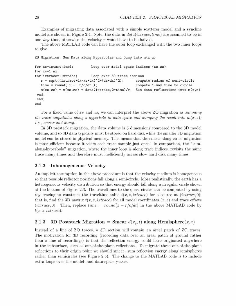
Examples of migrating data associated with a simple scatterer model and a synclinemodel are shown in Figure 2.4. Note, the data in data(ixtrace, time) are assumed to be inone-way time, otherwise the velocity v would have to be halved.

The above MATLAB code can have the outer loop exchanged with the two inner loopsto give

ZO Migration: Sum Data along Hyperbolas and Dump into m(x,z)

for xs=istart:iend; Loop over model space indices (xs,zs)

for zs=1:nz;

for ixtrace=1:ntrace; Loop over ZO trace indices

r = sqrt((ixtrace*dx-xs*dx)^2+(zs*dx)^2); compute radius of semi-circle

time = round( 1 + r/c/dt ); compute 1-way time to circle

m(xs,zs) = m(xs,zs) + data(ixtrace,2*time)/r; Sum data reflections into m(x,z)

end;

end;

end

For a fixed value of xs and zs, we can interpret the above ZO migration as summing

the trace amplitudes along a hyperbola in data space and dumping the result into m(x, z);i.e., smear and dump.

In 3D prestack migration, the data volume is 5 dimensions compared to the 3D modelvolume, and so 3D data typically must be stored on hard disk while the smaller 3D migrationmodel can be stored in physical memory. This means that the smear-along-circle migrationis most efficient because it visits each trace sample just once. In comparison, the ”sum-along-hyperbola” migration, where the inner loop is along trace indices, revisits the sametrace many times and therefore must inefficiently access slow hard disk many times.

2.1.2 Inhomogeneous Velocity

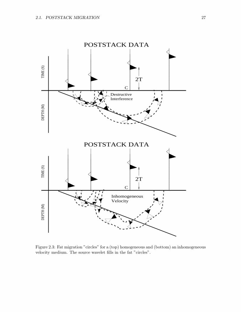
An implicit assumption in the above procedure is that the velocity medium is homogeneousso that possible reflector positions fall along a semi-circle. More realistically, the earth has aheterogeneous velocity distribution so that energy should fall along a irregular circle shownat the bottom of Figure 2.3. The traveltimes to the quasi-circles can be computed by usingray tracing to construct the traveltime table t(x, z, ixtrace) for a source at (ixtrace, 0);that is, find the 3D matrix t(x, z, ixtrace) for all model coordinates (x, z) and trace offsets(ixtrace, 0). Then, replace time = round(1 + r/c/dt) in the above MATLAB code byt(x, z, ixtrace).

2.1.3 3D Poststack Migration = Smear d(xg, t) along Hemisphere(x, z)

Instead of a line of ZO traces, a 3D section will contain an areal patch of ZO traces.The motivation for 3D recording (recording data over an areal patch of ground ratherthan a line of recordings) is that the reflection energy could have originated anywherein the subsurface, such as out-of-the-plane reflections. To migrate these out-of-the-planereflections to their origin point we should smear+sum reflection energy along semispheresrather than semicircles (see Figure 2.5). The change to the MATLAB code is to includeextra loops over the model- and data-space y-axes.


Destructive Interference

C

TIM

E (S

)D

EPTH

(M)

2T

POSTSTACK DATA

InhomogeneousVelocity

C

TIM

E (S

)D

EPTH

(M)

2T

POSTSTACK DATA

Figure 2.3: Fat migration ”circles” for a (top) homogeneous and (bottom) an inhomogeneousvelocity medium. The source wavelet fills in the fat ”circles”.


−0.5

0

0.5

1

X−offset (m)

Dep

th (m

)

Poststack Migration Image

0 200 400 600 800 1000 1200 1400 1600 1800

0

500

1000

1500

0

2

4

6

8

10

Offset (m)

Tim

e (s

)

Poststack AGC Data in 1−Way Time

0 200 400 600 800 1000 1200 1400 1600 1800

0

0.2

0.4

0.6

0.8

1

Student Version of MATLAB

0

5

10

15

20

Offset (m)

Tim

e (s

)


0 200 400 600 800 1000 1200 1400 1600 1800

0

0.2

0.4

0.6

0.8

1

−2

−1

0

1

2

3

X−offset (m)

Dep

th (m

)


0 200 400 600 800 1000 1200 1400 1600 1800

0

500

1000

1500


Figure 2.4: ZO traces and model generated by reflections from a (top 2 images) pointscatterer and (bottom 2 images) synclinal model denoted by white dashed lines. Migrationimage in red and blue colors is shown as well.


Non−ZO Trace

Prestack Migration Ellipsoid

*

ZO Trace

Poststack Migration Hemisphere

*

Figure 2.5: (Top) Poststack and (bottom) prestack migration impulse responses for 3Ddata.

3D MATLAB Poststack Migration Code

for ixtrace=1:ntrace; % Loop over ZO trace indices

for IYTRACE=1:ntrace;

for xs=istart:iend; % Loop over model space indices (xs,ys,zs)

for zs=1:nz; for YS=1:ny;

r = sqrt((ixtrace*dx-xs*dx)^2+(IYTRACE*dy-YS*dy)^2+(zs*dx)^2); % compute radius of

% hemi-sphere

time = round( 1 + r/c/dt ); % compute 1-way time to circle

m(xs,YS,zs) = m(xs,YS,zs) + data(ixtrace,IYTRACE,time)/r; % Smear and sum data

end % reflections into (x,z)

end;

end;

end

end

Note that there are almost twice as many end statements in the 3D code compared to the2D code, which means that 3D ZO migration is several orders of magnitude more expensivethan 2D ZO migration.


2.1.4 Obliquity Factor

An improved poststack image can be obtained by including an obliquity factor in the diffrac-tion stack equation:

m(x, z) =ntraces

∑

g=1

d̈ata(xg, t(xg, x, z))n̂ · r̂/||(x − xg)2 + z2||2, (2.2)

where n̂ is the unit normal at the surface and r̂ is the unit vector at the surface that is theincidence angle of the reflection ray between the trial image point and the geophone.

2.2 Prestack Migration

In a complex medium, such as beneath a salt dome, the NMO and stacking assumptionis inappropriate so that the stacked section is too blurred, and so cannot be well imagedby poststack migration. The cure to this problem is to eliminate the NMO and stackingsteps and perform prestack migration on the shot gather d(xg, 0, tg |xs, 0, ts) recorded on ahorizontal recording plane, where xg and xs denote the source and geophone x-coordinatesfor a shot gather. Here, tg and ts denote the listening time and source excitation time,respectively, and the source is typically assumed to be excited at time ts = 0.

2.2.1 Prestack Migration = Smear d(xg, t) along Ellipse(x, z)

Which parts of the model could the reflection energy at time τ originate from? Similarto the poststack migration example, the answer is that the (x, z) parts of the model thatsatisfy the moveout equation for a fixed t, xg and xs. This equation defines an ellipse inmodel space with foci at (xg, 0) and (xs, 0).

Similar to the poststack migration formula, prestack migration smears a reflection sam-ple into model space, but along the appropriate ellipse rather than a semi-circle. Theformula for prestack migration is given by

m(x, z) =∑

xg

∑

xs

d̈(xg, 0, τ(xg , xs, x, z)|xs, 0, ts)/A(x, z, xg , xs),

(2.3)

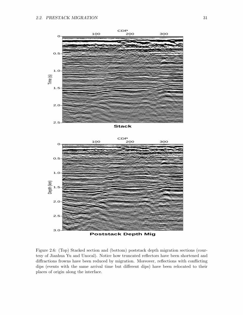
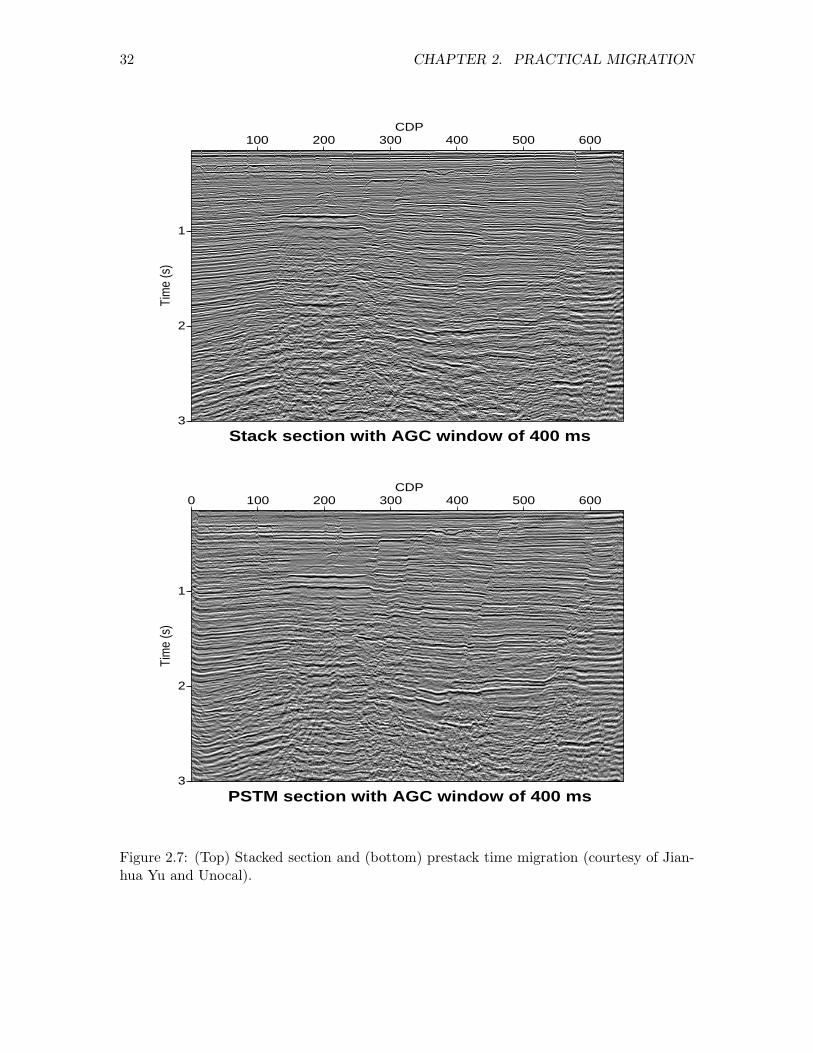
Examples of stacked data, poststack migration and prestack migration are given in Fig-ures 2.6-2.7.

2.2.2 Migration as a Pattern Matching Operation

The similiarity between two digital photos (each assumed to be a 100x100 pixelated imagein the x-y plane) can be quantified by representing each photo by a 10, 000x1 vector andtaking their dot product. If the photos are very similar then the dot product will yielda sum of mostly positive numbers to give a very high correlation coefficient. Conversely,the dot product between dissimilar photos will yield a sum of both positive and negativenumbers to give a small correlation coefficient. Taking dot products of photos is a commonpattern matching operation.

2.2. PRESTACK MIGRATION 31

0

0.5

1.0

1.5

2.0

2.5

Time (

s)

100 200 300CDP

Stack

0

0.5

1.0

1.5

2.0

2.5

3.0

Depth

(km)

100 200 300CDP

Poststack Depth Mig

Figure 2.6: (Top) Stacked section and (bottom) poststack depth migration sections (cour-tesy of Jianhua Yu and Unocal). Notice how truncated reflectors have been shortened anddiffractions frowns have been reduced by migration. Moreover, reflections with conflictingdips (events with the same arrival time but different dips) have been relocated to theirplaces of origin along the interface.


1

2

3

Tim

e (s

)

100 200 300 400 500 600 CDP

Stack section with AGC window of 400 ms

1

2

3

Tim

e (s

)

0 100 200 300 400 500 600 CDP

PSTM section with AGC window of 400 ms

Figure 2.7: (Top) Stacked section and (bottom) prestack time migration (courtesy of Jian-hua Yu and Unocal).

2.3. SPATIAL SAMPLING ISSUES 33

Summing the data over migration hyperbola in x − t space can also be thought of as apattern matching operation. The left image in Figure 2.8 depicts the migration curves inx − t space as solid curves, where each colored curve corresponds to a different trial imagepoint with the same color. Summing the data over a curve is equivalent to a 2-D dot productbetween the migration operator image and the data image. If the trial image point is nearthe actual scatterer, then the, e.g. black, migration operator in the left image of Figure 2.8matches the data very well. Hence, the migration image at that trial image point has a highvalue. At other trial image points, the pattern of the migration operator correlates poorlywith the data so the correlation is small to give a small value in the migration image.

2.2.3 Migration Operator for Multiple Arrivals

In theory, migrating many types of events with different arrival angles to their commonreflector point leads to a better resolution at that point, and a cleaner migration image.This is similar to looking at a diamond from different view angles, each new view anglerevealing a new facet of the gem.

To achieve this extra resolution with seismic images, one can tune a diffraction migra-tion operator to migrate both primary reflections and scattered multiples2 A representativemultiple migration operator is illustrated on the right hand side of Figure 2.8, where, fora trial image point, the summation of energy is along the hyperbolic curves (e.g., the solidblack curves) that represent the traveltimes for both primaries and multiples. For the cor-rect trial image point at the black dot, a huge of amount of seismic energy gets placedat the scatterer’s position by primary+multiple migration compared to that for primarymigration.

From a pattern matching point of view, the complicated pattern of the primary+multiplemigration operator correlates well with data only in a small neighborhood of the actualscatterer’s point; thus the image resolution is very good. Compare this to matching thesimple primary migration operator to the data; there is a relatively large neighborhoodaround the actual scatterer that gives a good match between the operator’s pattern andthe actual data. This means a migration image with worse resolution compared to theprimary+multiple migration image.

The disadvantage of primary+multiple migration is that its migration image is espe-cially sensitive to errors in the migration velocity model. Small migration velocity errorstend to give a noisier image compared to the primary migration image. In fact, the pri-mary+multiple migration operator can be shown to be identical to that for reverse timemigration, a subject to be discussed in a later chapter.

2.3 Spatial Sampling Issues

How does one choose the trace and shot intervals as well as the total recording aperture?The trace interval is selected so that the discrete representation of the data still containsunambiguous information about dips. Steeper data dips and higher source frequencies will

2A multiple migration algorithm can be constructed by ray tracing the traveltimes for both primaries and

multiples and including the extra summations in the diffraction stack migration formula.


Prim. Mig. Op. Prim.+Mult. Mig. Op.

Dashed curves = Primaries+Multiples Data

Solid curves = Primary Mig. Operator

Solid curves = Primary+Mult. Mig. Operator

Primary and Primary+Multiple Migration Operators

Figure 2.8: Migration of (left) primary and (right) primary+multiple reflection energy bydiffraction stack migration of data (dashed curves). The solid curves represent the migrationoperators for different trial image points (represented by filled circles in model space). Theprimary+multiple migration operator associated with the black trial image point providesthe best correlation between the ”dashed-data” photo and the ”black-migration-operator”photo.

2.3. SPATIAL SAMPLING ISSUES 35

demand finer trace spacing. Also, steeper dips in the model will give rise to ZO reflectionrays that are almost horizontal, so will demand wider recording apertures.

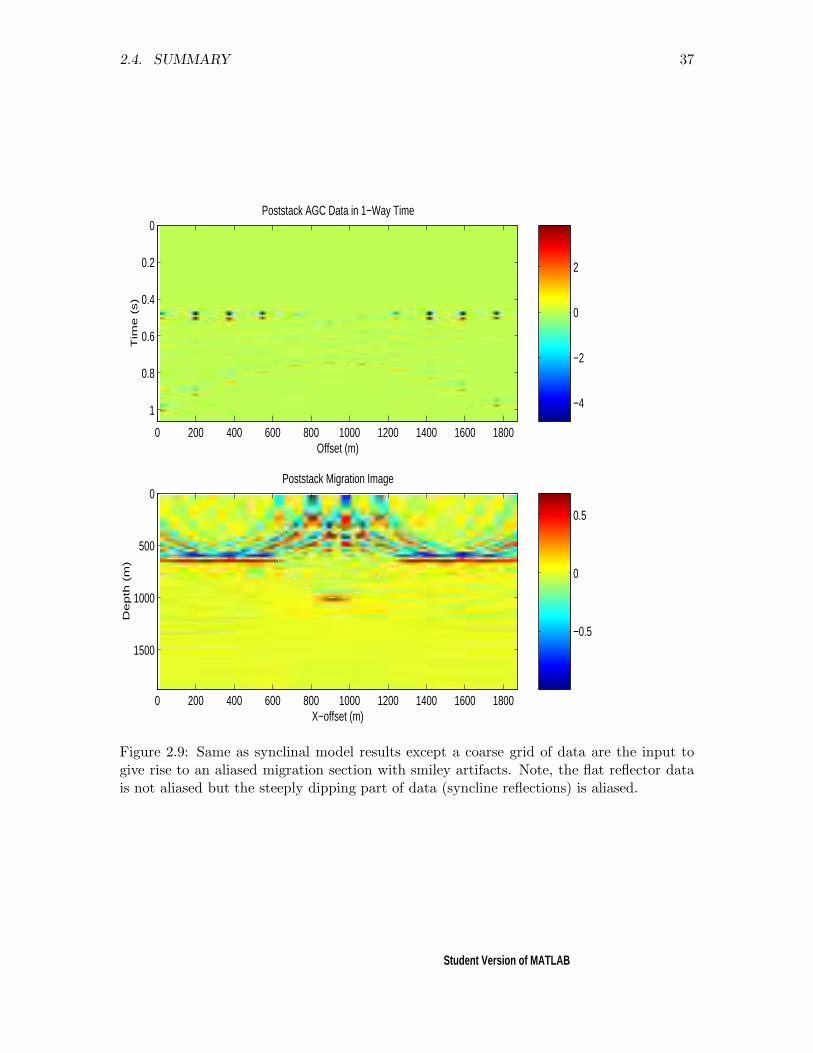
If the trace spacing is too coarse, the ”wings” of the hyperbolas will not completelycancel and so leave ugly smiles or frowns in the migration image, as shown in Figure 2.9.We say that the coarse trace spacing results in migration aliasing artifacts. Another pointof view is that steep dips in the data appear more shallow if the trace spacing is too coarse;i.e., the data are aliased..

Aliasing can be cured by making sure that the shortest apparent wavelength in the data(λx)min is greater than 1/2 the trace spacing ∆x. By definition min(λx) = Tmin(dx/dt)min

so that the anti-aliasing condition is

2∆x < min(λx) = (dx/dt)minTmin, (2.4)

where min(λx) is the minimum apparent wavelength along the x-direction in the hyperbolas.This is known as the Nyquist sampling criterion, and its violation means that neighboringtraces undergo more than 1/2 period of time shift. This assumes that the model grid isdiscretized finely enough to avoid problems in discretely sampling a continuous interface.

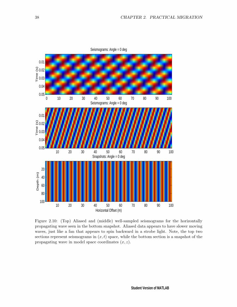
A visual example of aliased data is given in Figure 2.10. The bottom image is a snapshotof a horizontally propagating plane wave. The top and middle figures show the seismogramsrecorded on the horizontal surface, except the top section is aliased while the middle sec-tion is well sampled in space. The dip of the events in the middle section show the truepropagation velocity (dx/dt=v) while the apparent velocity of the dip in the top sectionis slower because the data are aliased. Try running the MATLAB code below to see howaliasing affects recorded data.

colormap(’gray’); subplot(311); plot(1:2,1:2); subplot(312);

plot(1:2,1:2); subplot(313); plot(1:3,1:3);

nangle=3;nt=50;nsnap=nt*nangle;itt=0;c=.2;

%%%%%%%%%%%%%%%%%%%%%%%%%%%%%%%%%%%%%%%%%%%%%%%%%%%%%

rect=get(gcf,’Position’);

rect(1:2)=[0 0];

M=moviein(nsnap,gcf,rect);

%%%%%%%%%%%%%%%%%%%%%%%%%%%%%%%%%%%%%%%%%%%%%%%%%%%%%

for iangle=1:nangle; lam=6;angle=pi/4.2*(iangle-1);

kx=2*pi*cos(angle)/lam;ky=sin(angle)*2*pi/lam;

nx=100;k=sqrt(kx^2+ky^2);w=k*c; r=1:1:nx;i=ones(nx,1);

dx=i*r; dy=dx’;tt=.001*[nt:-1:1];sei1=ones(nt,nx/4);

sei=ones(nt,nx);

for it=1:nt; itt=itt+1; pw=cos(dx*kx+dy*ky+w*it);pw=fliplr(pw);

for iii=1:25; sei1(it,iii)=pw(1,1+(iii-1)*4); end;

sei(it,:)=pw(1,:);

%%%%%%%%%%%%%%%%


subplot(311);

imagesc(r,tt,sei1);

if iangle==1;title(’Seismograms: Angle = 0 deg’);end;



ylabel(’Time (s)’); pause(.2)

%%%%%%%%%%%%%%%%

subplot(312);

imagesc(r,tt,sei);




ylabel(’Time (s)’); pause(.2)

%%%%%%%%%%%%%%%%

subplot(313);

imagesc(pw);xlabel(’Horizontal Offset (m)’);

ylabel(’Depth (m)’);

if iangle==1;title(’Snapshots: Angle = 0 deg’);end;



pause(.2)

%%%%%%%%%%%%%%%%

M(:,itt)=getframe(gcf,rect); end; end; N=1 ;

FPS=1 ;

movie(gcf,M,N,FPS,rect);

%mpgwrite(M, hot, ’filename’, [1, 0, 1, 0, 10, 8, 10, 25]);

2.3.1 Aperture Limitation.

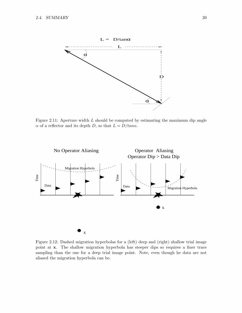
Wider apertures will lead to better horizontal resolution, and also allow for recording ofevents with nearly horizontal raypaths. The aperture width should be estimated by usingthe formula given in Figure 2.11.

2.4 Summary

The practical aspects of integral equation migration are reviewed. Migration can be viewedas either ”smearing a time sample of data along the corresponding migration circle (orellipse)”, or equivalently it can be viewed as ”summing energy along the appropriate hy-perbola (for a fixed trial image point at x and source-receiver pair) and dumping it intothe pixel centered at x”. The latter view is illustrated in Figure 2.12, where shallowertrial image points lead to more steeply dipping wings of the hyperbola. Since we are sum-ming amplitudes along these hyperbola we must ensure that the dip along the migrationhyperbola is not as steep as the trace spacing allows; otherwise the data are aliased.

2.4. SUMMARY 37

−0.5

0

0.5

X−offset (m)

De

pth

(m

)


0 200 400 600 800 1000 1200 1400 1600 1800

0

500

1000

1500

−4

−2

0

2

Offset (m)

Tim

e (

s)


0 200 400 600 800 1000 1200 1400 1600 1800

0

0.2

0.4

0.6

0.8

1


Figure 2.9: Same as synclinal model results except a coarse grid of data are the input togive rise to an aliased migration section with smiley artifacts. Note, the flat reflector datais not aliased but the steeply dipping part of data (syncline reflections) is aliased.


Seismograms: Angle = 0 deg

Tim

e (

s)

0 10 20 30 40 50 60 70 80 90 100

0.01

0.02

0.03

0.04

0.05

Seismograms: Angle = 0 deg

Tim

e (

s)

10 20 30 40 50 60 70 80 90 100

0.01

0.02

0.03

0.04

0.05

Horizontal Offset (m)

De

pth

(m

)

Snapshots: Angle = 0 deg

10 20 30 40 50 60 70 80 90 100

20

40

60

80

100


Figure 2.10: (Top) Aliased and (middle) well-sampled seismograms for the horizontallypropagating wave seen in the bottom snapshot. Aliased data appears to have slower movingwaves, just like a fan that appears to spin backward in a strobe light. Note, the top twosections represent seismograms in (x, t) space, while the bottom section is a snapshot of thepropagating wave in model space coordinates (x, z).

2.4. SUMMARY 39

L = D/tanα

L

D

α

α

Figure 2.11: Aperture width L should be computed by estimating the maximum dip angleα of a reflector and its depth D, so that L = D/tanα.

��

��

��

��

��

��

��

��

��

��

��

��

��

��

��

��

��

��

��

��

��

��

��

��

��

��

��

��

��

��

��

��

��

��

��

��

��

��

��

��

��

��

��

��

��

��

��

��

��

��

��

Tim

e

X

Tim

e

X

Data

Migration Hyperbola

Migration HyperbolaData

No Operator Aliasing Operator AliasingOperator Dip > Data Dip

Figure 2.12: Dashed migration hyperbolas for a (left) deep and (right) shallow trial imagepoint at x. The shallow migration hyperbola has steeper dips so requires a finer tracesampling than the one for a deep trial image point. Note, even though he data are notaliased the migration hyperbola can be.


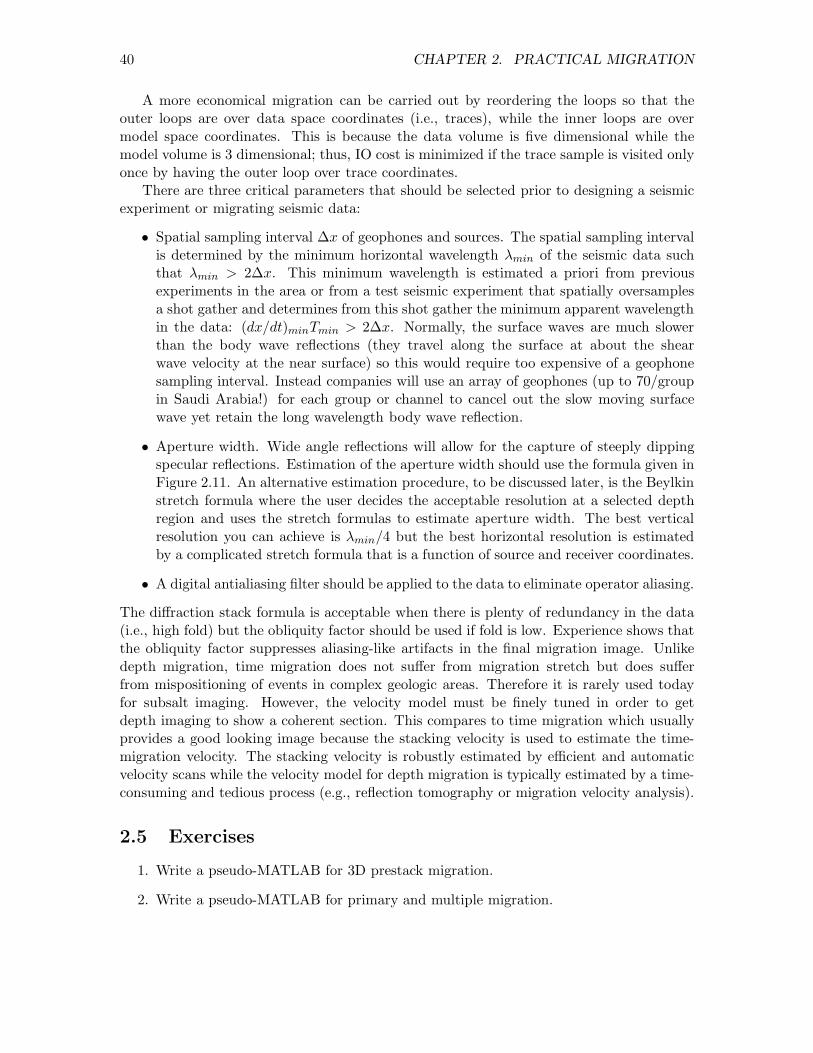
A more economical migration can be carried out by reordering the loops so that theouter loops are over data space coordinates (i.e., traces), while the inner loops are overmodel space coordinates. This is because the data volume is five dimensional while themodel volume is 3 dimensional; thus, IO cost is minimized if the trace sample is visited onlyonce by having the outer loop over trace coordinates.

There are three critical parameters that should be selected prior to designing a seismicexperiment or migrating seismic data:

• Spatial sampling interval ∆x of geophones and sources. The spatial sampling intervalis determined by the minimum horizontal wavelength λmin of the seismic data suchthat λmin > 2∆x. This minimum wavelength is estimated a priori from previousexperiments in the area or from a test seismic experiment that spatially oversamplesa shot gather and determines from this shot gather the minimum apparent wavelengthin the data: (dx/dt)minTmin > 2∆x. Normally, the surface waves are much slowerthan the body wave reflections (they travel along the surface at about the shearwave velocity at the near surface) so this would require too expensive of a geophonesampling interval. Instead companies will use an array of geophones (up to 70/groupin Saudi Arabia!) for each group or channel to cancel out the slow moving surfacewave yet retain the long wavelength body wave reflection.

• Aperture width. Wide angle reflections will allow for the capture of steeply dippingspecular reflections. Estimation of the aperture width should use the formula given inFigure 2.11. An alternative estimation procedure, to be discussed later, is the Beylkinstretch formula where the user decides the acceptable resolution at a selected depthregion and uses the stretch formulas to estimate aperture width. The best verticalresolution you can achieve is λmin/4 but the best horizontal resolution is estimatedby a complicated stretch formula that is a function of source and receiver coordinates.

• A digital antialiasing filter should be applied to the data to eliminate operator aliasing.

The diffraction stack formula is acceptable when there is plenty of redundancy in the data(i.e., high fold) but the obliquity factor should be used if fold is low. Experience shows thatthe obliquity factor suppresses aliasing-like artifacts in the final migration image. Unlikedepth migration, time migration does not suffer from migration stretch but does sufferfrom mispositioning of events in complex geologic areas. Therefore it is rarely used todayfor subsalt imaging. However, the velocity model must be finely tuned in order to getdepth imaging to show a coherent section. This compares to time migration which usuallyprovides a good looking image because the stacking velocity is used to estimate the time-migration velocity. The stacking velocity is robustly estimated by efficient and automaticvelocity scans while the velocity model for depth migration is typically estimated by a time-consuming and tedious process (e.g., reflection tomography or migration velocity analysis).

2.5 Exercises

1. Write a pseudo-MATLAB for 3D prestack migration.

2. Write a pseudo-MATLAB for primary and multiple migration.

2.5. EXERCISES 41

3. Which provides better horizontal resolution, near-offset or far-offset ZO traces; here,the offset refers to the horizontal offset from a buried scatterer. Explain answer withdiagrams.

4. The CDP interval in Figure 7 is 50 m. The velocity at z = 1 km is 2 km/s andat z = 2.5 km it is 4 km/s, and the recording aperture is 350 CDP’s wide for anyshot point. Calculate the minimum horizontal and vertical resolutions for a prestackmigration image at the points (x, z) = (0 km, 1 km), (x, z) = (1 km, 1 km), (x, z) =(0 km, 2.5 km), and (x, z) = (1 km, 2.5 km). Same question as before, except calculateminimum horizontal and vertical resolutions for a poststack migration image. Showwork.

5. Using fat circles and fat ellipses, compare the vertical and horizontal resolution limitsfor poststack migration and prestack migration for a point at (x, z) = (1 km, 2.5 km)in Figure 7. Assume a homogeneous velocity.

6. Convert your poststack depth migration code into a prestack time migration code.The output should be in the offset-time domain. Show poststack depth and timemigration images.

7. Determine the maximum aperture for a seismic experiment in order to image 0 − 40degree dips at z = 5 km. Assume a homogeneous velocity of 5 km/s. What isthe minimum geophone spacing in order to not spatially alias the data? Assume aminimum wavelet period of 0.01 s. Clearly show steps in your reasoning.

8. Estimate the horizontal wavelength of surface waves and body wave reflections in theSaudi shot gather (from a previous lab). What is a good array interval that wouldsuppress surface waves but retain body waves ion the data. Test your estimate byapplying an N-point spatial averaging filter to the data, where N is length of yourestimated filter. Show results.

diﬀraction stack migration 2 diﬀraction stack migration the basic assumption in resorting shot...

Documents