digital soil mapping using digital terrain analysis and ... · pdf filemeter resolution and...

Digital Soil Mapping Using Digital Terrain Analysis and

Statistical Modeling Integrated into GIS: Examples from

Vestfold County of Norway

Misganu Debella-Gilo1, Bernd Etzelmuller1, Ove Klakegg2

1University of Oslo, Institute of Geosciences, Sem Sælandsvei 1, 0371 Oslo, Norway Fax +47-22857230

E-mail: [email protected], [email protected],2Norwegian Institute of Forest and Landscape, Raveien 9, 1431 Ås, Norway

E-mail: [email protected]

Abstract. This paper outlines methodology to predict the spatial distribution of soil classes using digital terrain analysis and multinomial logistic regression for the Vestfold County of south-eastern Norway. A digital elevation model of 25 meter resolution and digitized soil map were used as original data for the terrain and soil respectively. Fifteen terrain attributes were derived from the digital elevation model. There were thirteen soil types in the surveyed area of the study site. The relationship between the soil types and the terrain attributes were modeled using multinomial logistic regression. The logit models were used to predict the probability of existence of each of the soil classes. The result showed that elevation, flow length, duration of daily direct solar radiation, slope, aspect and topographic wetness index were the most significant terrain attributes determining the spatial distribution of soil classes. The probability prediction for each soil class was found to be reliable when conceptually evaluated and visually compared against the empirical soil maps except for those which are not greatly influenced by topography but by other factors such as human activity.

Keywords: Digital soil mapping, terrain Analysis, GIS, logistic regression

1. Introduction

Digital Terrain Modeling has long replaced the qualitative and nominal characterization of topography. It has shown its comparative advantages in that it gives quantitative measurement of elevation, enables to derive any other terrain attribute quantitatively, enables to visualize topography in more realistic way than ever before, and enables to store, update, proliferate and manipulate topographic data digitally (Li et al., 2005; Moore et al., 1993; Wilson and Gallant, 2000a). It further provides the possibility of deriving indices that can be used as indicators for environmental processes (Pike, 1988; Wilson and Gallant, 2000b).

237

On the other hand, the role topography plays in bio-physical processes and phenomena is increasingly unraveled. One of such bio-physical process is pedogenesis, i.e. the soil formation process. Due to the fact that topography influences endogenic and exogenic soil forming factors and processes, it plays crucial role in the spatial distribution of soils and their properties (Schaetzl and Anderson, 2005). Furthermore, the characterization and investigation of the spatial distribution of soils and their properties, i.e. soil survey, is advancing due to the increasing need for knowledge about soils, triggered by their importance in the environmental well-being and agricultural activities. The conventional field investigation and laboratory analysis of soils at every site is becoming increasingly unaffordable in terms of financial cost, time and data deliverability. That is why other paradigms such as pedometrics and digital soil mapping are widening their scope and depending their applicability (McBratney et al., 2003).

Digital soil mapping involves quantitative prediction of soils and their properties using some observed soil data and auxiliary data on all or some soil forming factors (Dobos et al., 2006). During the prediction soil classes can be conceptualized as discrete objects with sharp spatial boundaries or as fuzzy variables with gradual spatial transition. However, naturally soils appear to be more of continuous variables than discrete objects (Qi et al., 2006a). Therefore, their conceptualization as discrete objects involves uncertainties. Such variables are best predicted through fuzzy logic approach so that the uncertainties related to conceptualization can be reduced. Application of fuzzy logic requires establishment of knowledge bases or models for the fuzzy membership criteria. For digital soil mapping, the fuzzy logic approach uses the principle that a spatial unit, e.g. a pixel, can contain soil which can not be exclusively classified into one soil class (Qi et al., 2006b). Membership values in fuzzy mapping can be determined using deterministic or empirical approaches.

The foundation of this research is that even if the spatial distribution of soils is dictated by five major factors, the influence of topography is so strong that it can be used to predict the spatial distribution of soils. Consequently, the value of the membership of each pixel to a given soil class can be determined as a function of the values of the topographic attributes for that pixel. The relationship between each terrain attribute and the probability of existence of each soil class may take the form of one of the curves of Fig. 1. With the exception of curve D, that represents sharp boundaries, as in the case of discrete approach, the others show non-linear relationship. The major part of the prediction is therefore to quantitatively model this relationship between the probability of existence of a soil class and terrain attributes.

Since directly building such a non-linear model is not simple, a model that linearises the relationship is required. The best of such models is the logit model, built through logistic regression. Logit model relates the natural logarithm of the odds (ratio of the probability of existence to that of non-existence) to the predictor variables (Menard, 2002). Logit model is preferred because it is less demanding in terms of the behavior of the data sets such as normality, constant moments, etc (Menard, 2002; Raimundo et al., 2006 ). In cases where the dependent categorical variable has more than two categories, the multinomial version of the logistic regression is applied.

238 Proceedings, ScanGIS’2007

Figure 1 Graphical depiction of some of the possible relationship between a predictor and the class optimality value

The objective of this paper is to produce digital map of soil classes as fuzzy variables whereby the fuzzy memberships are estimated through probability values modeled using logistic regression of the World Reference Base soil groups against terrain attributes. This pilot study was carried out for parts of the Vestfold county of South-eastern Norway.

2. Setting

This research was conducted in Vestfold County, in the southern part of Norway. The area extends over the municipalities of Sandefjord, Larvik, Andebu, and partly those surrounding them. It covers an area of 1835 square kilometer (35 km by 52 km), centering around 59º N and 10º E (Fig. 2). The area was selected based on the availability of most of the necessary data and its representativeness for the majority of the Norwegian agricultural landscape, especially those below the marine line. Vestfold is the second smallest of the nineteen Norwegian counties. However, it has the highest proportion of agricultural land compared to all the other counties (Nyborg and Solbakken, 2003). The favorability of the area for agriculture is due to the fact that the area lies today in what has been a glacier marginal zone during the last glaciation, leading to accumulation of glacigenic and marine sediments.

3. Methods

3.1. Data

Digital Elevation Model (DEM) of the area at the resolution of 25m, which was created by the Norwegian Mapping Authority, based on triangulation of 20 m contour maps, road and river data. The absolute accuracy of the DEM is given as ±5 to 6 m. The

Sample Soil Maps were obtained from Norwegian Institute of Forest and Landscape. The institute conducted the classification and the mapping of the soils there in the field

Debella-Gilo, Etzelmuller and Klakegg 239

following a modified version of the FAO field guide, FAO (WRB) soil classification system and soil mapping procedures (Nyborg and Solbakken, 2003). They used stereo aerial photographs of the areas to delineate soil units in the field. The soil unit maps were digitized using an AP190 Analytical Plotter and converted to SOSI and ESRI file formats. There were 13 soil classes found in the surveyed area whose spatial distribution is displayed in Fig. 3 together with their area coverage. Besides, Anthropic Regosol is added as a separate class due to its unique characteristics.

The Satellite Images: The Enhanced Landsat Thematic Mapper image from May 2000 was used to mask areas covered by water bodies such as lakes and sea. The image was radiometrically corrected and geometrically orthorectified by NASA (Tucker et al., 2004)

Figure 2 The Vestfold county and the study area

Figure 3 Spatial distribution of the soil classes in the study area. Numbers in brackets show the proportion of the soil type’s spatial coverage of the surveyed area.


3.2. Digital Terrain Analysis

Pre-Evaluation and Pre-Processing of the DEM. Apart from the accompanying standard error report, there are some acceptable procedures (Li et al., 2005; Liu et al., 2006; Wise, 2002; Zhou and Liu, 2004) used to evaluate the overall quality of DEM. First, the histograms of the elevation data itself and that of aspect were investigated. Second, the shaded relief of the DEM was visually investigated to see artificial structures. Third, depression and spikes were derived from the DEM and investigated to identify if they are natural lakes or artificially introduced sinks. Artificial depressions were removed from the DEM using (Planchon and Darboux, 2002; Planchon, 2001) method accompanied with drainage enforcement in flat areas. Spikes, i.e. unusually high elevated pixels in relation to their surroundings, were also removed. All the subsequent analytical procedures were applied on the so smoothed DEM.

Derivation of Terrain Attributes. A number of primary and secondary terrain attributes were derived using ARCGIS and TAS (Terrain Analysis Systems) developed by John Lindsey of the University of Manchester (John, 2005). In Table 1, the definition, methods used to derive the values and the units of the terrain attributes used in this research are given. The formulae used in the table are based on figure 4 which is modified from (Gallant and Wilson, 2000; Wilson and Gallant, 2000b).

Figure 4 A three by three grid showing how to calculate surface derivatives (Gallant and Wilson, 2000)

3.3. Statistical Modeling of the Continuous Relationship between Soil Classes

and Terrain Attributes

First, all the maps of the terrain attributes and the soil classes were projected to the same reference system, i.e. WGS 84 UTM 32N. Then the values of the terrain attributes and the soil classes were extracted into a table for all the areas covered by the sample soil map. Considering the soil classes as categorical dependent variable and the terrain attributes as quantitative predictor variables, logistic regression was applied in SPSS. The multinomial logistic regression (NOMREG) module of the SPSS was employed as the dependent variable had more than two categories. When employing NOMREG, one of the soil classes, Umbrisol, was defined as reference category. The Chi-square based maximum likelihood ratio test was used to evaluate the overall model fit and to estimate the significance of each terrain attribute in influencing the spatial distribution of the soil class. The significance of the regression coefficient of each predictor variable for each dependent variable was evaluated using the Wald statistic.


All the main effect, factorial and stepwise options were employed until the best model significance was obtained.

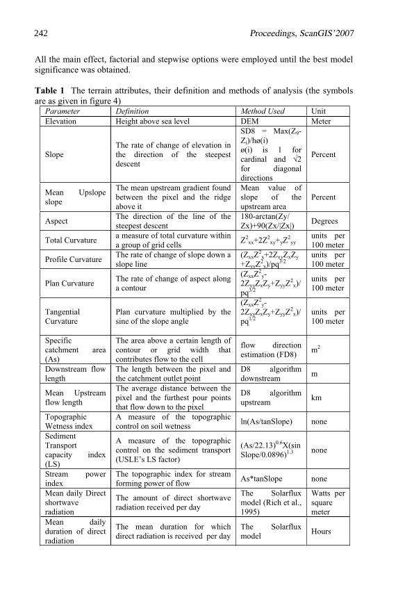
Table 1 The terrain attributes, their definition and methods of analysis (the symbols are as given in figure 4)

Parameter Definition Method Used UnitElevation Height above sea level DEM Meter

SlopeThe rate of change of elevation in the direction of the steepest descent

SD8 = Max(Z9-Zi)/hø(i)ø(i) is 1 for cardinal and 2for diagonal directions

Percent

Mean Upslope slope

The mean upstream gradient found between the pixel and the ridge above it

Mean value of slope of the upstream area

Percent

Aspect The direction of the line of the steepest descent

180-arctan(Zy/ Zx)+90(Zx/|Zx|)

Degrees

Total Curvature a measure of total curvature within a group of grid cells

Z2xx+2Z2

xy+yZ2

yyunits per 100 meter

Profile Curvature The rate of change of slope down a slope line

(ZxxZ2

x+2ZxyZxZy

+ZyyZ2

y)/pq3/2units per 100 meter

Plan Curvature The rate of change of aspect along a contour

(ZxxZ2

y-2ZxyZxZy+ZyyZ

2x)/

pq3/2

units per 100 meter

Tangential Curvature

Plan curvature multiplied by the sine of the slope angle

(ZxxZ2

y-2ZxyZxZy+ZyyZ

2x)/

pq1/2units per 100 meter

Specific catchment area (As)

The area above a certain length of contour or grid width that contributes flow to the cell

flow direction estimation (FD8)

m2

Downstream flow length

The length between the pixel and the catchment outlet point

D8 algorithm downstream

m

Mean Upstream flow length

The average distance between the pixel and the furthest pour points that flow down to the pixel

D8 algorithm upstream

km

TopographicWetness index

A measure of the topographic control on soil wetness

ln(As/tanSlope) none

SedimentTransportcapacity index (LS)

A measure of the topographic control on the sediment transport (USLE’s LS factor)

(As/22.13)0.6X(sinSlope/0.0896)1.3 none

Stream power index

The topographic index for stream forming power of flow

As*tanSlope none

Mean daily Direct shortwave radiation

The amount of direct shortwave radiation received per day

The Solarflux model (Rich et al., 1995)

Watts per squaremeter

Mean daily duration of direct radiation

The mean duration for which direct radiation is received per day

The Solarflux model

Hours


The identification of whether a terrain attribute has significant relation with the distribution of a soil type is expressed through the significance of the coefficient of that terrain attribute in the logit of the given soil class. Second, the idea of how it is related and the extent of the relationship is not a straight forward issue to interpret. It is the exponent of the coefficients (EXP(B)), often called the odds ratio, that is most suitable for such interpretation. It is suitable because it indicates the factor by which odds ratio of the category increases when a terrain attribute is increased by one unit (Menard, 2002; Peng et al., 2002). Odds ratio is greater than 1 indicate that the probability of occurrence increases due to increase in the values of the predictor variable, and there is positive correlation between the factor and the probability that the dependent variable exists. On the other hand, EXP(B) less than 1 indicate negative correlation between the predictor and the dependent variables. EXP(B) value of 1 indicates that increase by one unit of the terrain attribute does not influence the odds ratio. The farther away the EXP(B) is from 1, the stronger the influence is. However, the magnitude has no direct indication of the change in the probability values (Menard, 2002).

3.4. Probability Mapping Using Multinomial Logistic Regression model

The logit is the logarithmic function of the ratio between the probability that a pixel is a member of a class (P) divided by the probability that it is not (1-P). Its value can be directly predicted from the predictor values through regression as:

Logiti = ln(Pi/(1-Pi)) = a + b1X11+ b2X2+…. + bnXn + (1)

The equation shows how to calculate the logit of a category, e.g. soil class i, predicted from a number of quantitative factors X1…n, e.g. terrain attributes. The ‘a’ indicates the intercept of the regression curve, the ‘b’s are the coefficients of each predictor, and represents random and systematic (if any) error. From this equation it is possible to derive:

Pi = e a + b1X1+ b2X2+….+ bnXn +

1 + 1m-1(e a + b1X1+ b2X2+…. + bnXn) (2)

This equation is used to predict the probability P that a soil class i is present at a pixel given the levels of the terrain attributes X1, X2, …, Xn, by dividing the logit of i to that of the total sum of the logits of all other soil classes (except the reference category) plus unity (Menard, 2002). One of the classes, often the last in the list, is considered as reference and its logit is not estimated. However, its probability of existence is given as:

Pr = __1______________________ +

1 + 1m-1(e a + b1X1+ b2X2+…. + bnXn) (3)

The values of the ‘a’ and the ‘b’s have to be determined for each soil class based on empirical data. Once the values have been estimated with statistical significance (which


is out of the scope of this article to discuss), models 2 and 3 can be integrated into a GIS tool to map the probability that a given soil class i is found at a given pixel based on the values of the terrain attributes X1…n.

Logit models for each soil class were constructed using the terrain attributes that were found to be significant by the Wald statistic test for that soil class and their respective coefficient. The logit models were related to the probability models as in equation 2. Besides, equation 3 was used to predict the probability of the reference category. These probability models of the soil groups were fed into the raster calculator of ARCGIS to produce a map showing the probability of existence at each pixel for each soil class.

The prediction of soils and their properties from terrain attributes based on soil-landscape modeling involves huge amount of data with different sources and lengthy analytical procedures. At every stage, starting from the conceptualization to data acquisition to analysis, there are uncertainties involved. Here, uncertainties might be involved in the terrain data, soil data, their spatial definition, analytical procedures, etc. Therefore, the reliability of the outputs needs to be evaluated one way or another.

The ideal way of assessing the reliability of the prediction would have been by comparing the predicted probability values with the actual probability values. However, the actual probability values do not exist. The reference soil map itself is a vector map created based on discrete classification concept and contains uncertainties. Had the database on which the models were built been soil profiles which are representative of just one soil class, the profiles would have been given probability value of 1 and the deviation of the prediction from those would have easily been calculated as an indicator of the accuracy.

Nonetheless, expert knowledge and the “rule of thumb” approach were used to evaluate the reliability of the results. Some soil classes develop under restrictively defined landscapes. Using this fact and expert judgment of the spatial distribution of soils in the area, the landscape over which each predicted soil class has high probability values was evaluated. Besides, the predicted maps were visually compared to the empirical map of each soil class of the area published by Solbakken et al. (2006).

4. Results

4.1. The Soil Terrain Relations as Modeled by Logistic Regression

The overall multinomial logistic model was found to be significantly fit at p<0.05. Table 2 further shows that the most significant terrain attributes in influencing the spatial distribution of the soil classes were found to be elevation, downstream flow length, mean daily duration of radiation, mean upslope slope, slope aspect, etc in descending order. In fact, with the exception of plan curvature all of the terrain attributes were found to be significantly influential.


Table 2 The significance of each terrain attribute in the overall model Likelihood Ratio Tests

Model fitting criteria

Likelihood Ratio Tests Effect

-2 Log Likelihood of Reduced Model

Chi-Square

Degrees of freedom

Sig.

Elevation 223469.33 18769.14 13.00 0.00

Downstream flow length

215214.89 10514.70 13.00 0.00

Mean daily duration of radiation

206495.91 1795.72 13.00 0.00

Mean upslope slope 205509.50 809.32 13.00 0.00

Slope 205030.49 330.30 13.00 0.00

Aspect (sin.cos) 204857.72 157.53 13.00 0.00

Received Mean daily direct radiation

204836.65 136.46 13.00 0.00

Upstream flow length 204802.35 102.16 13.00 0.00

Specific catchment area 204786.02 85.83 13.00 0.00

Wetness Index 204773.80 73.61 13.00 0.00

Erosion Index (LS) 204754.32 54.13 13.00 0.00

Relative Stream Power Index

204754.30 54.11 13.00 0.00

Tangent Curvature 204732.28 32.10 13.00 0.00

Total Curvature 204729.45 29.26 13.00 0.01

Profile curvature 204725.98 25.79 13.00 0.02

Plan Curvature 204 667.44 16.54 13.00 0.22

On the other hand, the terrain attributes which were found significantly influential in the spatial distribution of each soil class and the type and extent of the influences are presented in table 3. Almost all soil classes were found to be influenced by at least two terrain attributes. The least influenced soil type is found to be Anthrosol, followed by Leptosol. The magnitudes in the table indicate the factor by which the odds ratios of the soil classes change if the value of the given terrain attribute is increased by a unit. Values greater than 1 indicate that increase in the values of the terrain attribute results in the increase in the probability of that soil class, although the magnitude has no meaning in that regard. On the other hand, values less than 1 show the opposite of this. The further the values are from 1, the stronger the influence is. This will be discussed in detail later as it needs some caution.

The other outcome of the analysis is the possibility of constructing logit models for each soil class except for the reference soil class (table 4). Each model enables to predict the probability that a given soil class exists in a given area given the values of the terrain attributes which are found to be significantly influential in the spatial distribution of that soil class. More correctly, the models linearly relate terrain attributes to the logit of the soil classes. The coefficient B shows the linear change in the logit of the soil class when a terrain attribute is increased by a unit value. Since it is


linearly related to the logit, it is used to construct the logit model for each soil class in analogy with a multiple linear regression. One can look at the models presented in table 3 to know how the logit of each soil class is related to a particular terrain attribute.

Table 3 The influence of each terrain attribute on each soil class as expressed in odd ratios

Parameter Estimates

Predictor EXP(B) of Soil class

AB AR AT CM FL GL HS LP LV PH PZ RGRGah

Aspect(sin.cos) 1.39 0.27 1.35 1.17 0.48 1.90 TotalCurvature 0.13 Downstream Flow Length 1.01 1.01 1.01 1.01 1.01 1.01 1.01 0.99 1.01 0.99 0.99 1.01 0.99

Elevation 0.99 0.91 0.98 0.95 0.98 0.99 1.01 1.05 0.98 1.02 1.00 1.01 0.97 Topographicerosion index (LS) 1.12 1.12

slope 0.93 1.05 0.86 0.86 0.85 0.92 0.85 Profilecurvature 0.10 MeanUpslopeslope 0.99 0.96 0.96 0.99 1.02 0.97 0.99 Relativestream power index 1.00 0.99 0.99 Specific catchment area 0.99 0.99 0.99 0.99 0.99 Tangentialcurvature 0.03 Upstream flow length 1.01 1.01 1.00 1.01 1.01 Wetness index 0.99 0.95 0.98 1.04 0.96 Meanduration of direct radiation 0.72 3.21 0.62 0.37 0.81 0.59 0.50 0.75 1.74 0.70 Meandirectshortwaveradiation 1.00 1.00 1.00 1.00 1.00 1.00 1.00 1.00


Table 4 The logit models of the soil classes as expressed by the terrain attributes. (Note that the units are as expressed in table 1)

Soil class Logit model Albeluvisol 0.325 * [aspectsincos] + 0.31 * [curve_total] + 0.002 * [downstr._flow_length] - 0.011

* [elevation] + 0.75 * [profile curve] - 0.012 * [upslope_slope] - 0.066 * [slope] Anthropic Regosol

7.723 + 0.639 * [aspectsincos] - 0.001 * [downstr._flow_length] - 0.034 * [elevation] - 0.014 * [upslope_slope] - 0.040 * [slope] + 0.006 * [upstr._flow_length] - 0.362 * [mean_radiation_duration]

Anthrosol - 15.12 - 1.32 * [aspectsincos] + 0.001 * [mean_radiation_duration] - 0.024 * [elevation] - 0.091 * [slope] - 0.045 * [wetness_index] + 1.146 * [mean_radiation_duration]

Arenosol 5.81 + 0.002 * [downstr._flow_length] - 0.098 * [elevation] - 0.72 * [profilecurv] - 0.04 * [upslope_slope] - 0.03 * [slope] + 0.007 * [upstr._flow_length] - 0.014 * [wetness_index] - 0.323 * [mean_radiation_duration]

Cambisol 6.8 + 0.296 * [aspectsincos] + 0.002 * [downstr._flow_length] - 0.048 * [elevation] - 0.434 * [profilecurv] - 0.038 * [upslope_slope] - 0.047 * [slope] + 0.006 * [upstr._flow_length] - 0.473 * [mean_radiation_duration]

Fluvisol 9.42 + 1.04 * [curve_total] + 0.001 * [downstr._flow_length] - 0.018 * [elevation] + 0.111 * [ls] + 1.6 * [profilecurv] - 0.008 * [upslope_slope] - 0.008 * [rsp] - 0.182 * [slope] + 0.004 * [upstr._flow_length] - 0.999 * [mean_radiation_duration]

Gleysol 2.88 + 0.745 * [curve_total] + 0.001 * [downstr._flow_length] - 0.009 * [elevation] + 0.124 * [ls] + 2.178 * [profilecurv] - 0.015 * [rsp] - 0.256 * [slope] - 0.222[mean_radiation_duration]

Histosol 5.008 + 1.209 * [curve_total] + 0.001 * [downstr._flow_length] + 0.006 * [elevation] + 2.334 * [profilecurv] + 0.023 * [upslope_slope] - 0.207 * [slope] + 0.021 * [wetness_index] - 0.544 * [mean_radiation_duration]

Leptosol - 0.004 * [downstr._flow_length] + 0.050 * [elevation] Luvisol 2.730 + 0.152 * [aspectsincos] + 0.496 * [curve_total] + 0.001 *

[downstr._flow_length] - 0.022 * [elevation] + 1.264 * [profilecurv] - 0.081 * [slope] - 0.016 * [wetness_index]

Phaeozem 10.332 - 0.706 * [aspectsincos] - 0.004 * [downstr._flow_length] + 0.024 * [elevation] - 0.135 * [slope] - 0.712 * [mean_radiation_duration]

Podzol 4.632 - 0.001 * [downstr._flow_length] + 0.004 * [elevation] - 0.032 * [upslope_slope] + 0.010 * [upstr._flow_length] - 0.040 * [wetness_index] - 0.285 * [mean_radiation_duration]

Regosol -9.309 + 0.001 * [downstr._flow_length] + 2.324 * [profilecurv] - 0.148 * [slope] + 0.543 * [mean_radiation_duration]

4.2. Automated Spatial Prediction of Soil Types and its Performance

Figures 5 to 7 show the probabilities that a given soil class is located in a given pixel with values between 0 and 1, where 0 is absolutely no chance and 1 indicates sure existence of the soil. The red areas show the high probability areas for that soil class. With the exception of Anthrosols and Regosols the maximum probability values of all the other soil classes were above 0.5. The maps were found to be very reliable when evaluated using the two approaches explained in the methodology part of this article. Evaluation of the maps based on the generic definition of the soil classes and comparison with the empirical soil map indicated that high probability areas for a soil class more or less coincided with areas covered with that soil class in the empirical map.

The five groups listed below fit well with the theory of the spatial distribution of soil classes and correlated visually well with the empirical soil map.


1. Soils with high probability on the hills and steep areas: These are Leptosols dowelling the hill tops and Umbrisols and Podzols dowelling steep areas. 2. Soils with high probabilities in the valleys and very gentle slopes: these are Cambisols, Fluvisols, Luvisols, and Albeluvisols. 3. Soils with high probabilities at the depressions and beach playas: These are Gleysols and Arenosols 4. Soils that correlated most with vegetated areas but on flat to gentle slopes: these are Histosols and Phaeozems 5. Soils with unreliable topographic relations: Anthrosols, Regosols and Anthropic Regosols.

The selected maps themselves further testify the reliability of the method in different ways. Figure 5 shows two soil groups, i.e. Albeluvisols and Arenosls, which are different in their origin and generic properties such as texture. Their probability distribution distinguished these soils strikingly. The high probability values of both soils are located where they are theoretically expected and empirically found. Figure 6 two soil groups, i.e. Cambisols and Leptosols, which are known to dwell different topographic zones. The prediction also testified to this fact. On the other hand, figure 7 shows two soil groups, i.e. Anthrosols and Regosols, whose probability values tell us that they do not exit in the area. One has to look at the area coverage of these soils in figure 3 to confirm this. They each cover only 0.1% of the surveyed area. Besides, the fact that Anthrosols is dictated by human activity than topography resulted in very limited correlation of this soil with topographic parameters. Each of this soil groups are accompanied by other soil groups as stated in the five groups presented earlier due to the similarity in their topographic characteristics.

Figure 5 The probability distribution of Albeluvisols (left) and Arenosols (right). Notice that the sandy soil (Arenosol) has high probability values around the beach, where as Albeluvisol dominates gentle slopes above the marine line.


Figure 6 The probability distribution of Cambisols (left) and Leptosols (right). Notice the striking topographic difference, i.e. Leptosols occupying the hills and rocky areas and Cambisols occupying the valleys.

Figure 7 The probability distribution of Anthrosol (left) and Regosol (right). Notice the low probability values due to the almost non-existence of these soils in the area.


5. Discussion

The logistic regression analysis employed in this research came up with a number of useful results: (1) The analyses showed which terrain attributes are generally influential in the spatial distribution of soils (table 2). The reason as to why some terrain attributes are very influential is related to the fact that they influence the spatial distribution of radiation, temperature, moisture and flux of materials (Hugget and Cheesman, 2002). The only insignificant attribute was found to be the plan curvature, which is the rate of change of aspect. The influence of this parameter is more represented by tangential curvature

which includes local slope in the calculation (Gallant and Wilson, 2000). (2) The result also enabled to identify which terrain attributes influence the continuous spatial variation of each soil class and the extent of its influence. This is evaluated through the odds ratios (EXP(B)) of the terrain attributes for each soil class. One has to be cautious in comparing the EXP(B) of one terrain attribute to the other because they are simply not on the same scale. Notice that some terrain attributes have odds ratios, i.e. EXP(B) far away from 1 (e.g. aspect, curvature) while others have either 1 or close to it (e.g. elevation, flow length, etc) for most soil classes. Such differences are created due to two possible reasons: first, due to the fact that one terrain attribute actually has greater or less effect on the soil class than the other. Second, the unit value of one terrain attribute is practically larger than that of the other. For example, a unit of elevation is a measure which does not dramatically change the probability of any soil class. Where as, a one degree change in curvature can create big differences both in the type of soil and its properties. Therefore, one has to be reminded of the unit values of the terrain attribute when looking at the odds ratios of each terrain attribute. This was the reason why terrain attributes with large values were converted to a unit that can reduce the magnitude. For example, the unit of flow length was converted from meter to kilometer to cope with this situation as a one unit change in the predictor needs to be meaningful (Peng et al., 2002). However, what is more important is whether the odds ratio is greater than 1 which corresponds to the positive correlation of the linear regression, or less than 1 which corresponds to the negative correlation of the linear regression. (3) It further helped to construct prediction models which enabled to predict the spatial distribution of the probability of finding each soil type in the study area. Based on the sample data used for the model construction, it is evident that the terrain is more suitable for the development of some soil classes, while it is less so for others. This applies to the very low maximum probability values predicted for the almost non-present soil class in the study area, i.e. Regosols. Furthermore, the results of multinomial logistic regression is known to be biased by the proportion of the samples (Peng et al., 2002; Raimundo et al., 2006). Since the proportion of the samples in this research was not even, it may have had impact on the result. Finally, the spatial distribution of some soil classes is less dictated by topography than other bio-physical factors, making their prediction from terrain attributes difficult. Typical examples of such soil classes are Anthrosols and Anthropic Regosols which are results of human activities.


The sample soil class data that was used for the analysis was obtained as vector map of the soil classes. Each polygon of a soil class is basically assigned probability value of 1 for that soil class and 0 for the other soil classes. The problem is that this probability values are not based on actual observed values, since the polygons are assigned to the soil classes based on the observations made at a point within the polygon. The point might contain exclusively a given soil class, but it is unlikely that the entire polygon is exclusively of that soil class. Therefore, the assumed empirical data is not actually observed data but combination of observed and inferred data. Had the whole data set been soil class data from point observation, they would have been considered free of uncertainties and the uncertainties of the prediction would have been straight forward to estimate. The error estimation could have been done by subtracting the predicted probabilities of the observed points from 1 (the observed probability value).

Geospatial analysis involves uncertainties during conceptualization, representation, measurement, analysis and interpretation (Lark and Bolam, 1997; Longley et al., 2005). A number of possible sources of error can be pointed out for this particular research. The main uncertainties are related to (1) the digital elevation model quality, (2) the pixel resolution generalization, (3) errors related to the derivation of the terrain attributes, (4) the collection of soil information and delineation of their boundaries, and (5) the statistical analysis. One has to be aware of the uncertainties and the actual information content of the outputs so that the uncertainties during interpretation of the final result are reduced.

Nonetheless, the approaches used to evaluate the reliability of the predictions worked fine as they enabled to relate the prediction to the theories of soil genesis (FAO, 1998) and to the actual spatial distribution of the soil classes in the study area (Solbakken et al., 2006). Consequently, the first group of the probability correlation consists of soil classes which are known to develop in areas where there is accumulation of organic matter which requires the presence of wetness due to flooding or poor internal drainage. The second group contains soil classes known to dwell on flat and gently sloping areas with pedogenically favorable conditions. The third group, Umbrisols and Podzols, are found basically under the same physical environment that is subjected to bleaching and eluviation, but they differ in that the second contains high organic matter. Anthrosols and Anthropic Regosols of the fourth group correlated not due to their generic nature but due to the fact that they are both results of human activity and human activities tend to be dominant in certain topography. Leptosols are outstanding because they are basically thin soil cover over outcropping rocks that are expressions of hill tops. Phaeozems of this area seem to occupy unique environment.

6. Conclusions

This research has exemplified how digital terrain analysis can be used for digital soil mapping. The following conclusions are made based on the outcome of this research and might only hold for this study area:

All soil types are influenced at least by two terrain attributes to a certain extent. The most influential terrain attributes as obtained from the logistic regression

analysis are elevation, flow length, slope, mean daily duration of radiation, aspect and


topographic wetness index. These parameters are believed to govern the distribution of moisture, temperature, radiation and flux of material which in turn dictate pedogenesis within the scale frame of this study.

Digital terrain analysis can effectively be used to make fuzzy digital maps of soils. In this regard, probability prediction using logit models of logistic regression are robust in terms of their reliability and flexibility to certain data constraints. They produce reliable results of prediction for most soil classes except for those which are influenced more by other factors such as human activity than topography. The reliability of the prediction for most of the soil classes and its failure for the soil classes which have little relation to topography are testimonies for the reliability of the method. However, the prediction could even be improved if information on land use, geology and vegetation cover is included together with improved sample qualities, size and spatial distribution.

Acknowledgements

This study was part of a M.Sc. study carried out at the Laboratory of Remote Sensing and GIS at the Department of Geosciences, University of Oslo (Bernd Etzelmüller), in close collaboration with the Norwegian Institute of Forest and Landscape (Arnold Arnouldsen, Ove Klakegg). The authors want to express their gratitude to the mentioned institutions.

References

Dobos, E., Carré, F., Hengl, T., Reuter, H.I. and Tóth, G., 2006. Digital Soil Mapping as a support to production of functional maps. EUR 22123 EN. Office for Official Publications of the European Communities, Luxemburg, 68 pp.

FAO, 1998. World reference base for soil resources. FAO, ISRIC and ISSS, Rome. Gallant, J.C. and Wilson, D.J., 2000. Primary topographic attributes. In: D.J. Wilson and J.C.

Gallant (Editors), Terrain Analysis: Principles and Applications. John Willey & Sons, INC, New York, pp. 51-85.

Hugget, R. and Cheesman, J., 2002. Topography and the Environment. Pearson Education Limited, Harlow.

John, B.L., 2005. The Terrain Analysis System: a tool for hydro-geomorphic applications, pp. 1123-1130.

Lark, R.M. and Bolam, H.C., 1997. Uncertainty in prediction and interpretation of spatially variable data on soils. Geoderma, 77(2-4): 263-282.

Li, Z., Zhu, Q. and Gold, C., 2005. Digital Terrain Modeling: Principles and Methodology. CRC Press, Boca Raton.

Liu, T.L., Juang, K.W. and Lee, D.Y., 2006. Interpolating soil properties using kriging combined with categorical information of soil maps. Soil Science Society of America Journal, 70(4): 1200-1209.

Longley, P.A., Goodchild, M.F., Maguire, D.J. and Rhind, D.W., 2005. Geographical Information Systems and Science Wiley, Chichester.

McBratney, A.B. and Odeh, I.O.A., 1997. Application of fuzzy sets in soil science: fuzzy logic, fuzzy measurements and fuzzy decisions. Geoderma, 77(2-4): 85-113.


McBratney, A.B., Santos, M.L.M. and Minasny, B., 2003. On digital soil mapping. Geoderma, 117(1-2): 3-52.

Menard, S.S., 2002. Applied Logistic Regression Analysis. Quantitative applications in the social sciences. Sage Publications, Thousand Oaks.

Moore, I.D., Grayson, R.B. and Ladson, A.R., 1993. Digital terrain modeling: a review of hydrological, geomorphological, and biological applications. In: K.J. Beven and I.D. Moore (Editors), Terrain Analysis and Distributed Modeling in Hydrology. Advances in Hydrological Processes. John Wiley & Sons, INC, Chichester.

Nyborg, Å.A. and Solbakken, E., 2003. Klassifikasjonssystem for jordsmonn i Norge: Feltguide basert på WRB. NIJOS dokument (6).

Peng, C.Y.J., So, T.S.H., Stage, F.K. and John, E.P.S., 2002. The use and interpretation of logistic regression in higher education journals: 1988-1999. Research in Higher Education, 43(3): 259-293.

Pike, R.R., 1988. THE GEOMETRIC SIGNATURE - QUANTIFYING LANDSLIDE-TERRAIN TYPES FROM DIGITAL ELEVATION MODELS. Mathematical Geology, 20(5): 491-511.

Planchon, O. and Darboux, F., 2002. A fast, simple and versatile algorithm to fill the depressions of digital elevation models. Catena, 46(2-3): 159-176.

Planchon, O.C., 2001. A fast, simple and versatile algorithm to fill the depressions of digital elevation models. Catena, 46(2-3): 159.

Qi, F., Zhu, A.X., Harrower, M. and Burt, J.E., 2006a. Fuzzy soil mapping based on prototype category theory. Geoderma, 136(3-4): 774-787.

Qi, F., Zhu, A.X., Harrower, M. and Burt, J.E., 2006b. Fuzzy soil mapping based on prototype category theory. Geoderma, In Press, Corrected Proof.

Raimundo, R., Barbosa, A.M. and Vargas, J.M., 2006. Obtaining Environmental Favorability Functions from Logistic Regression. Environmental and Ecological Statistics, V13(2): 237-245.

Raimundo, R., Barbosa, A.M. and Vargas, J.M., 2006 Obtaining Environmental Favorability Functions from Logistic Regression. Environmental and Ecological Statistics, 3 (2): 8.

Rich, P.M., Hetrick, W.A. and Saving, S.C., 1995. Modeling Topographic influences on Solar Radiation: A manual for the SOLARFLUX model. Los Alamos National Laboratory, Los Aamos, New Mexico.

Schaetzl, R.J. and Anderson, S., 2005. Soils: genesis and geomorphology. Cambridge University Press, Cambridge, XIII, 817 s. pp.

Solbakken, E., Nyborg, Å., Sperstad, R., Fadnes, K. and Klakegg, O., 2006. Jordmonnsatlas for Norge. Viten fra Skog og Landskap, 01. Norsk Institut for Skog og Landskap, Ås.

Tucker, C.J., Grant, D.M. and Dykstra, J.D., 2004. NASA's global orthorectified landsat data set. Photogrammetric Engineering and Remote Sensing, 70(3): 313-322.

Wilson, D.J. and Gallant, J.C., 2000a. Digital terrain analysis. In: D.J. Wilson and J.C. Gallant (Editors), Terrain Analysis: Principles and Applications. John Willey & Sons, INC, New York, pp. 1-27.

Wilson, P.J. and Gallant, J.C., 2000b. Secondary topographic attributes. In: P.J. Wilson and J.C. Gallant (Editors), Terrain Analysis: Principles and Applications. John Willey & Sons, INC, New York, pp. 87-131.

Wise, S., 2002. Terrain analysis - Principles and applications. International Journal of Geographical Information Science, 16(7): 711-712.

Zhou, Q.M. and Liu, X.J., 2004. Error analysis on grid-based slope and aspect algorithms. Photogrammetric Engineering and Remote Sensing, 70(8): 957-962.


digital soil mapping using digital terrain analysis and ... · pdf filemeter resolution and...

Documents