remote sensing based estimates of surface wetness

Boreal environment research 16: 407–416 © 2011issn 1239-6095 (print) issn 1797-2469 (online) helsinki 31 october 2011

remote sensing based estimates of surface wetness conditions and growing degree days over northern alberta, canada

m. shammi akther and Quazi K. hassan*

Department of Geomatics Engineering, Schulich School of Engineering, University of Calgary, 2500 University Dr NW, Calgary, Alberta T2N1N4, Canada (corresponding author’s e-mail: [email protected])

Received 18 Oct. 2010, accepted 17 Dec. 2010 (Editor in charge of this article: Hannele Korhonen)

akther, m. s. & hassan, Q. K. 2011: remote sensing based estimates of surface wetness conditions and growing degree days over northern alberta, canada. Boreal Env. Res. 16: 407–416.

Here, our aims are to estimate two most important climate-driven variables of the surface wetness condition (SWC) and growing degree days (GDD: a temperature regime) prima-rily using remotely sensed 8-day composites from Moderate-resolution Imaging Spectrom-eter (MODIS) sensor over the agriculture and forest-dominated regions in the Canadian province of Alberta. The estimation of both SWC and GDD was based on exploiting relations between surface temperature and vegetation indices. Our results showed that on average in 81.67% of the cases, the MODIS-derived SWC values differed less that ±20% from the ground-based measurements of volumetric soil moisture. The MODIS-derived GDD values differed less ±20% from the ground-based measurements of GDDs in 90.39% of the cases.

Introduction

It is well recognized that climate-driven vari-ables are critical for both agriculture and forestry (Cosh et al. 2010, Latta et al. 2009, Palm et al. 2010). Two most important such variables are the surface wetness condition (SWC, indirectly indicating soil moisture (SM), i.e. the amount of water in the soil column available to plants); and growing degree days (GDD). These variables are crucial for vegetation growth and many plant functions (e.g., photosynthesis, transpiration, both plant and soil respiration, water and nutri-ent movements within plant, etc.) (Flanagan and Johnson 2005, Hari and Nöjd 2009). They both can be measured precisely in situ using various methods. However, the ground-based methods

fail to provide the spatial variability, which is important for understanding the dynamics at the landscape scale. One of the feasible alternatives are remote sensing methods, which have already been proven to address the spatial dynamics for the variables of interest (Anttila and Kairesalo 2010, Sekhon et al. 2010, Stenberg et al. 2008).

For the last two decades, visible and ther-mal infrared remote-sensing data were widely used to determine SWC. In most cases, SWC can be derived from the relationships between the vegetation index (VI) and the actual surface temperature (Ts) (Carlson 2007, Li et al. 2009, Patel et al. 2009). A two dimensional scatter plot of Ts-VI usually assumes a triangular (Sandholt et al. 2002, Carlson 2007) or a trapezoidal shape (Moran et al. 2004, Petropoulos et al. 2009). The

408 Akther & Hassan • Boreal env. res. vol. 16

edges of these shapes are considered in estimat-ing SWC (see section Estimation of TVWI below for more details). In general, the negative slope of the Ts-VI diagram describes the water avail-ability with respect to the vegetation conditions, e.g., (i) high SWC values are found for relatively dense vegetation with low Ts values; and (ii) low SWC values are found for sparse vegetation with high Ts values. To describe the VI component, the normalized difference vegetation index (NDVI: as a function of surface-reflectance values from red and near-infrared spectra; Parviainen et al. 2010) is used. The Ts-VI space can be defined by using either daily or composite values. However, Venturini et al. (2004) emphasized uncertainty of the daily Ts values acquired by means of remote sensing resulting from atmospheric conditions. They also mentioned that the use of a multiday (e.g., 14- or 16-day) composite of Ts would not be useful for their proposed method of deter-mining f (i.e., the combined effects of Prestley-Taylor’s α and Budyko-Thronwaite-Mather’s wetness parameters) as a part of estimating eva-potranspiration by using the Ts-VI relation. Other researchers (e.g., Patel et al. 2010, Chen et al. 2010) used composites in the Ts-VI approach for determining SWC regimes, and demonstrated their effectiveness.

Despite the wider acceptability of the Ts-VI method, the major limitation is its applicability over a topographically variable terrain (Carlson 2007), and the fact that it has not been widely used over vegetated regions. The topographic-variability limitation was first addressed by Hassan et al. (2007b) for the forest-dominated humid region in the Canadian Atlantic Maritime Ecozone. It was done by transforming Ts into a potential surface temperature (θs), i.e. Ts with removed effect of elevation by recalculating the temperateure at the site for the mean sea level, and then combining it with NDVI (the method described as the temperature-vegetation-wetness index, TVWI) (Hassan et al. 2007b, Hassan and Bourque 2009). However, the TVWI approach requires further validation over other ecozones to determine its wider applicability.

On the other hand, several studies demon-strated that remote sensing data were also effec-tive in calculating GDD as a function of remote-sensing based Ts (Hassan et al. 2007a, 2007c,

Neteler 2010). In Hassan et al. (2007a, 2007c), the initial step was to convert the MODIS-based 8-day composites of Ts (acquired between 10:30 and 12:00) into 8-day mean values using an empirical relationship. This relationship was built by using ground-based emitted longwave radiation data (by way of applying Stefan-Boltz-man’s equation; Langer et al. 2010). In reality, such longwave radiation data might be difficult to avail in other places. Thus, we propose to convert the MODIS-based Ts by establishing an empirical relation between Ts and the ground-based air temperature (Ta) measured at the mete-orological stations within the area of interest. In theory, the availability of such meteorological stations is relatively better across the globe (the networks of Ameriflux, fluxnet-Canada, Car-boEurope, Chinaflux, etc.).

In this paper, we aim: (i) to implement the TVWI approach over the topographically-vari-able agriculture and forest-dominated northern portion of the Canadian province of Alberta, and to assess its ability of capturing the ground-based measured volumetric soil moisture (VSM); (ii) to calculate GDDs over the growing season (i.e., April–October) by integrating MODIS-based Ts and ground-based Ta, and evaluating the mod-eled GDD by comparing it with the ground-based measured GDD.

Study area and data requirements

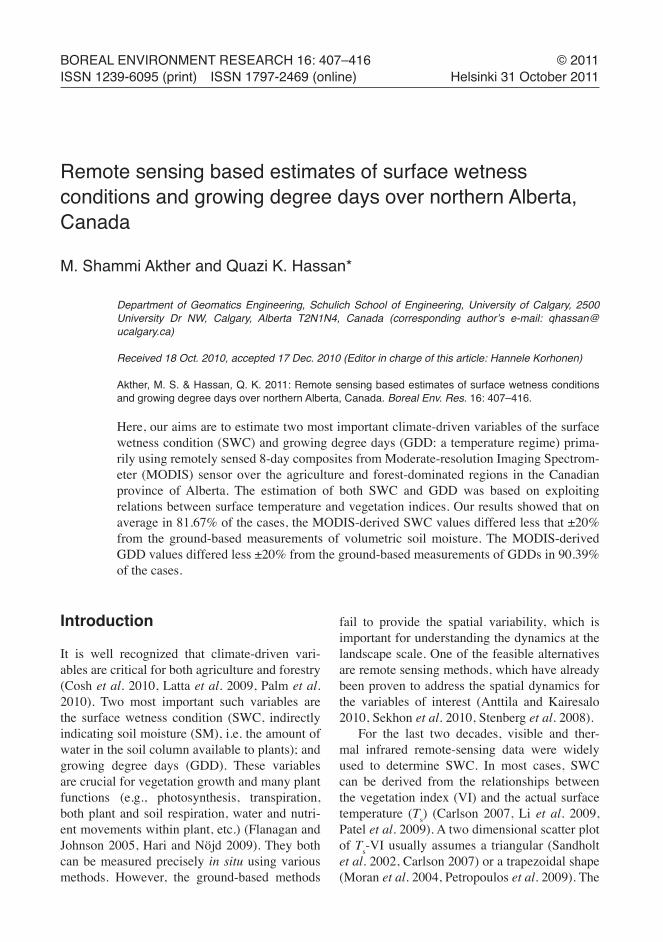
The extent of the study area is geographically between 53°–60°N and 108°–120°W (Fig. 1). It falls into the northern portion of the Canadian province of Alberta. It can be characterized as topographically variable (i.e., average elevation varies from 225 m to 1750 m a.s.l.) with the dominance of agriculture and forest land-cover types (see Fig. 1 for more details). The average annual temperature across the study area varies between –3.6 and +2.3 °C; the mean annual pre-cipitation varies between 300–900 mm (Dowing and Pettapiece 2006).

In this study, we primarily used Moderate Resolution Imaging Spectroradiometer (MODIS based products freely available from the Land Processes Distributed Active Archive Center (LP DAAC: a component of NASA’s earth observing

Boreal env. res. vol. 16 • Surface wetness and growing degree days in Alberta, Canada 409

system data and information system) (https://lpdaac.usgs.gov/lpdaac/products/modis_prod-ucts_table). Those included: (i) MOD11A2 ver. 005: 8-day composites of Ts (generated by aver-aging the clear-sky daytime Ts values over 8-day periods) at 1-km resolution in April–October 2005–2008; (ii) MOD09Q1 ver. 005: 8-day com-posites of red (620–670 nm) and near-infrared (NIR: 841–876 nm) surface reflectance at 250 m resolution in May–September 2006–2008; (iii) MOD13Q1 ver. 005: 16-day composite of EVI (enchanced vegetation index) at 250-m resolu-tion during April–October 2005–2008. We also used a digital elevation model (DEM) of the study area at 250-m resolution generated from 3-arc-second resolution height point-data freely available from the NASA Shuttle Radar Topog-raphy Mission archive (http://srtm.csi.cgiar.org). In addition, we used ground-based measurements of daily mean: (i) Ta from 77 stations, freely available from Environment Canada (http://cli-mate.weatheroffice.ec.gc.ca); (ii) VSM from 13 stations (5-cm, 20-cm, 50-cm and 100-cm depths acquired using Theta-Probe-type ML2x), freely available from Alberta Agriculture and Rural Development Department (http://www.agric.gov.ab.ca/app116/stationview.jsp) for the same period as the remote sensing data; and (iii) long-term (i.e., 1971–2000) average GDD data from 52 stations, freely available from Environment Canada (http://climate.weatheroffice.ec.gc.ca).

Methodology

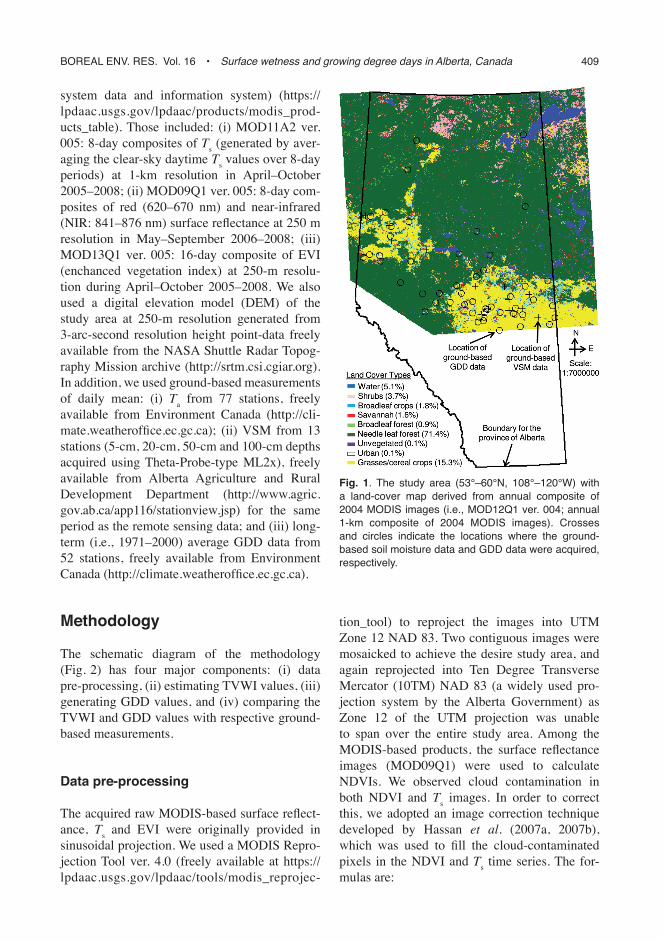
The schematic diagram of the methodology (Fig. 2) has four major components: (i) data pre-processing, (ii) estimating TVWI values, (iii) generating GDD values, and (iv) comparing the TVWI and GDD values with respective ground-based measurements.

Data pre-processing

The acquired raw MODIS-based surface reflect-ance, Ts and EVI were originally provided in sinusoidal projection. We used a MODIS Repro-jection Tool ver. 4.0 (freely available at https://lpdaac.usgs.gov/lpdaac/tools/modis_reprojec-

tion_tool) to reproject the images into UTM Zone 12 NAD 83. Two contiguous images were mosaicked to achieve the desire study area, and again reprojected into Ten Degree Transverse Mercator (10TM) NAD 83 (a widely used pro-jection system by the Alberta Government) as Zone 12 of the UTM projection was unable to span over the entire study area. Among the MODIS-based products, the surface reflectance images (MOD09Q1) were used to calculate NDVIs. We observed cloud contamination in both NDVI and Ts images. In order to correct this, we adopted an image correction technique developed by Hassan et al. (2007a, 2007b), which was used to fill the cloud-contaminated pixels in the NDVI and Ts time series. The for-mulas are:

Fig. 1. the study area (53°–60°n, 108°–120°W) with a land-cover map derived from annual composite of 2004 moDis images (i.e., moD12Q1 ver. 004; annual 1-km composite of 2004 moDis images). crosses and circles indicate the locations where the ground-based soil moisture data and GDD data were acquired, respectively.


, and (1)

, (2)

where A is the average deviation of either Ts or NDVI from their respective ’s for a specific cloud-contaminated pixel of interest, is the 8-day composite mean value of either Ts or NDVI for a specific year for the entire image, i is the 8-day period of interest, and n is the total number of 8-day composite images in a year; xi the image-based Ts or NDVI value from cloud-free 8-day composites, m is the total number of cloud-free pixels from individual composite images available for a specific year for a cloud-contaminated pixel, and B is the estimated 8-day mean of either Ts or NDVI for an individual cloud-contaminated pixel.

Estimation of TVWI

The estimation of TVWI was performed in two steps proposed by Hassan et al. (2007b): (i)

converting the Ts into θs; and (ii) interpreting the observed scatter plots of θs–NDVI.

To convert Ts into θs, the following expres-sions were used (Hassan et al. 2007b, Hassan and Bourque 2009):

, (3)

, (4)

where p is the atmospheric pressure (kPa), z is the elevation above the mean sea level (m), Ts is the actual surface temperature (K); po is the aver-age pressure at the mean sea level (= 101.3 kPa), R is the gas constant (= 287 J kg–1 K–1), Cp is the specific heat capacity of air (~1004 J kg–1 K–1), and θs is the potential surface temperature (K).

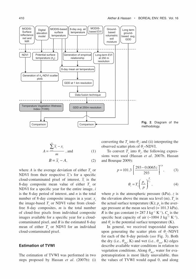
In general, we received trapezoidal shapes upon generating the scatter plots of θs–NDVI for each of the 8-day periods (see Fig. 3). Both the dry (i.e., θdry, K) and wet (i.e., θwet, K) edges describe available water conditions in relation to vegetation conditions. Along θdry, water for eva-potranspiration is most likely unavailable, thus the values of TVWI would equal 0, and along

Digital elevation

model

MODIS-Surface

reflectance red and

NIR

Temperature Vegetation Wetness Index (TVWI)

MODIS-based surface

temperature

Comparison

NDVI Potential surface temperature (θs)

8-day avg. air temperature

Generation of θs-NDVI scatter plots

Ground-based

volumetric soil

moisture

Long term ground-

based avg. GDD

8-day mean air temperature

GDD at 1 km resolution

Comparison

MODIS-based EVI

Long-term EVI at 250 m

resolution

GDD at 250m resolution

Data fusion technique

Generation of empirical relationship

Fig. 2. Diagram of the methodology.


θwet, water for evapotranspiration is unrestricted, thus the values of TVWI would equal 1.

Finally, TVWI is calculated using the follow-ing expression (Hassan et al. 2007b, Hassan and Bourque 2009):

, (5)

Generation of GDD

In generating GDD maps, the following steps were carried out: (i) converting the MODIS-based instantaneous 8-day composites of Ts into the equivalent 8-day mean Ta, and calculating the GDD values at 1-km resolution; and (ii) enhanc-ing the spatial resolution of the GDD map from 1 km to 250 m, so that it would be consistent with the spatial resolution of the TVWI maps.

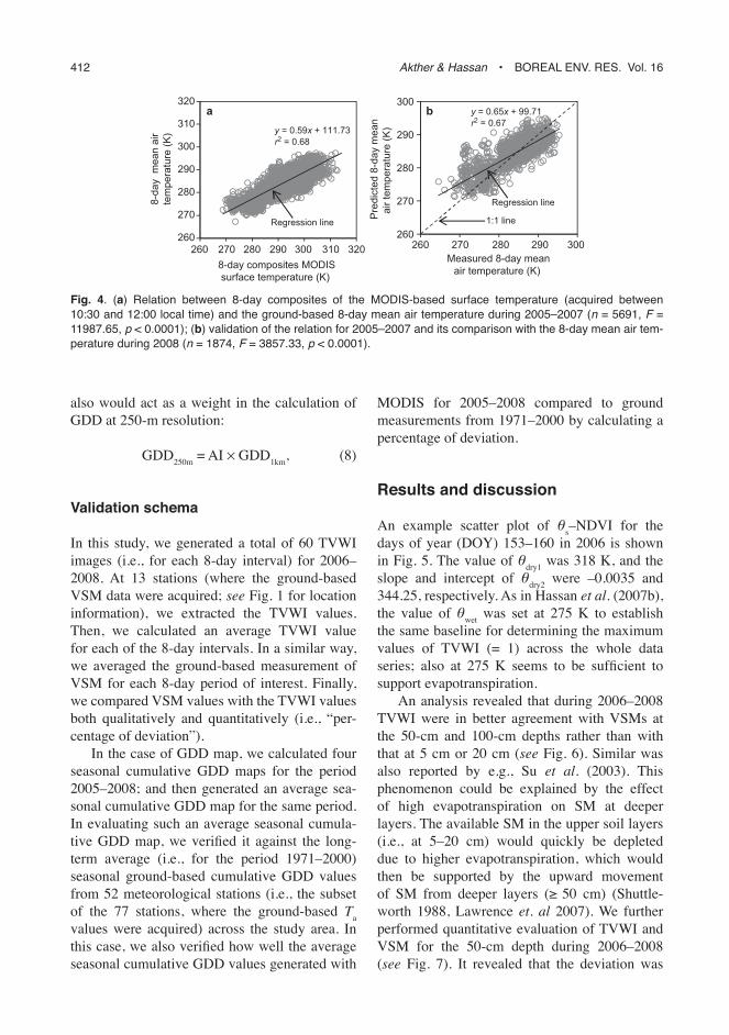
The daily mean Ta values from 77 meteoro-logical stations (see Fig. 1 for location informa-tion) were transformed into 8-day means for the same 8-day periods as the MODIS data. For those stations, we also extracted the MODIS-based instantaneous 8-day composites of Ts. Then, using Microsoft Excel 2007, we per-formed a linear-regression analysis for these two variables (see Fig. 4a). It revealed that a reasonably strong relation existed (r2 ≈ 0.68, slope = 0.59 ± 0.01, intercept = 111.73 ± 3.09 at 95% confidence level for the regression line, p < 0.0001) during the period 2005–2007. In order to evaluate how the function given in Fig. 4a can predict the 8-day mean Ta, we used this rela-tion to calculate Ta using 8-day MODIS-based Ts for 2008. The analysis revealed that also this relationship was reasonabley strong (r2 ≈ 0.67, slope = 0.65 ± 0.021, intercept = 99.71 ± 5.83 at 95% confidence level for the regression line, p < 0.0001) between the measured and predicted values (see Fig. 4b). Both phases (calibration and validation, see Fig. 4) demonstrated simi-lar levels of agreement (i.e., r2 ≈ 0.67), and the discrepancies (≈33% of the cases) were due to the fact that the Ta values were acquired at point locations but the MODIS-based Ts values were averages for 1 ¥ 1 km2 areas.

Considering the above, using the function given in Fig. 4a, we calculated equivalent 8-day mean Ta values. We then used these values in

the following expression to calculate seasonally accumulated GDDs:

, (6)

where Tbase equals 5 °C (= 278.15 K), and i and n are the first and the last 8-day period of the growing season, respectively, for which the 8-day mean Ta values were calculated.

As the initial spatial resolution of the Ts data was 1 km, the generated GDDs would also be at the same resolution. In order to enhance their spatial resolution, we used the EVI images at the 250-m resolution for data fusion as described in Hassan et al. (2007c). Such fusion was possible as the variables of EVI and GDD were found to be ecologically-related (Hassan et al. 2007a). With this method, an artificial image (AI) was generated for a 3 ¥ 3 moving window:

(7)

where EVIins is the instantaneous value of EVI in the center of the moving window, and EVImean is the mean of all the EVI values within the moving window. In theory, AI is an index that explains the relation of an instantaneous value of EVI to the mean value of EVI within a given window. It

Maximum transpiration

Normalized difference vegetation index (NDVI)

Dry edge,θdry-1 = c1

Maximum evaporation

TVWI = 1

TVWI = 0

Wet edge, θwet

No transpiration

Pot

entia

l sur

face

tem

pera

ture

(θs)

(NDVI, θs)

Dry edge,θdry-2 = mNDVI + c1

Noevaporation

TVWI =θdry – θsθdry – θwet

Fig. 3. conceptual diagram illustrated the calculations of tvWi as a function of θs and nDvi. Both of the dry edge (i.e., θdry) and wet edge (i.e., θwet) would describe the available water conditions in relation to vegetation conditions. c1 is the dry edge for θdry1; m and c2 are the slope and intercept for θdry2, respectively. modified after hassan et al. 2007b.


also would act as a weight in the calculation of GDD at 250-m resolution:

GDD250m = AI ¥ GDD1km, (8)

Validation schema

In this study, we generated a total of 60 TVWI images (i.e., for each 8-day interval) for 2006–2008. At 13 stations (where the ground-based VSM data were acquired; see Fig. 1 for location information), we extracted the TVWI values. Then, we calculated an average TVWI value for each of the 8-day intervals. In a similar way, we averaged the ground-based measurement of VSM for each 8-day period of interest. Finally, we compared VSM values with the TVWI values both qualitatively and quantitatively (i.e., “per-centage of deviation”).

In the case of GDD map, we calculated four seasonal cumulative GDD maps for the period 2005–2008; and then generated an average sea-sonal cumulative GDD map for the same period. In evaluating such an average seasonal cumula-tive GDD map, we verified it against the long-term average (i.e., for the period 1971–2000) seasonal ground-based cumulative GDD values from 52 meteorological stations (i.e., the subset of the 77 stations, where the ground-based Ta values were acquired) across the study area. In this case, we also verified how well the average seasonal cumulative GDD values generated with

MODIS for 2005–2008 compared to ground measurements from 1971–2000 by calculating a percentage of deviation.

Results and discussion

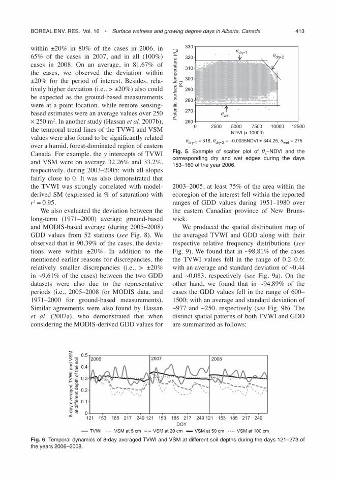
An example scatter plot of θs–NDVI for the days of year (DOY) 153–160 in 2006 is shown in Fig. 5. The value of θdry1 was 318 K, and the slope and intercept of θdry2 were –0.0035 and 344.25, respectively. As in Hassan et al. (2007b), the value of θwet was set at 275 K to establish the same baseline for determining the maximum values of TVWI (= 1) across the whole data series; also at 275 K seems to be sufficient to support evapotranspiration.

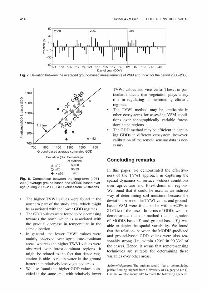
An analysis revealed that during 2006–2008 TVWI were in better agreement with VSMs at the 50-cm and 100-cm depths rather than with that at 5 cm or 20 cm (see Fig. 6). Similar was also reported by e.g., Su et al. (2003). This phenomenon could be explained by the effect of high evapotranspiration on SM at deeper layers. The available SM in the upper soil layers (i.e., at 5–20 cm) would quickly be depleted due to higher evapotranspiration, which would then be supported by the upward movement of SM from deeper layers (≥ 50 cm) (Shuttle-worth 1988, Lawrence et. al 2007). We further performed quantitative evaluation of TVWI and VSM for the 50-cm depth during 2006–2008 (see Fig. 7). It revealed that the deviation was

260

270

280

290

300

310

260

270

280

290

300

260

1:1 line

Regression line

8-day composites MODISsurface temperature (K)

8-da

y m

ean

air

tem

pera

ture

(K)

Measured 8-day meanair temperature (K)

Pre

dict

ed 8

-day

mea

nai

r tem

pera

ture

(K) y = 0.59x + 111.73

r2 = 0.68

y = 0.65x + 99.71r2 = 0.67

a b

Regression line

270 280 290 300260 270 280 290 300 310 320

320

Fig. 4. (a) relation between 8-day composites of the moDis-based surface temperature (acquired between 10:30 and 12:00 local time) and the ground-based 8-day mean air temperature during 2005–2007 (n = 5691, F = 11987.65, p < 0.0001); (b) validation of the relation for 2005–2007 and its comparison with the 8-day mean air tem-perature during 2008 (n = 1874, F = 3857.33, p < 0.0001).


within ±20% in 80% of the cases in 2006, in 65% of the cases in 2007, and in all (100%) cases in 2008. On an average, in 81.67% of the cases, we observed the deviation within ±20% for the period of interest. Besides, rela-tively higher deviation (i.e., > ±20%) also could be expected as the ground-based measurements were at a point location, while remote sensing-based estimates were an average values over 250 ¥ 250 m2. In another study (Hassan et al. 2007b), the temporal trend lines of the TVWI and VSM values were also found to be significantly related over a humid, forest-dominated region of eastern Canada. For example, the y intercepts of TVWI and VSM were on average 32.26% and 33.2%, respectively, during 2003–2005; with all slopes fairly close to 0. It was also demonstrated that the TVWI was strongly correlated with model-derived SM (expressed in % of saturation) with r2 = 0.95.

We also evaluated the deviation between the long-term (1971–2000) average ground-based and MODIS-based average (during 2005–2008) GDD values from 52 stations (see Fig. 8). We observed that in 90.39% of the cases, the devia-tions were within ±20%. In addition to the mentioned earlier reasons for discrepancies, the relatively smaller discrepancies (i.e., > ±20% in ~9.61% of the cases) between the two GDD datasets were also due to the representative periods (i.e., 2005–2008 for MODIS data, and 1971–2000 for ground-based measurements). Similar agreements were also found by Hassan et al. (2007a), who demonstrated that when considering the MODIS-derived GDD values for

2003–2005, at least 75% of the area within the ecoregion of the interest fell within the reported ranges of GDD values during 1951–1980 over the eastern Canadian province of New Bruns-wick.

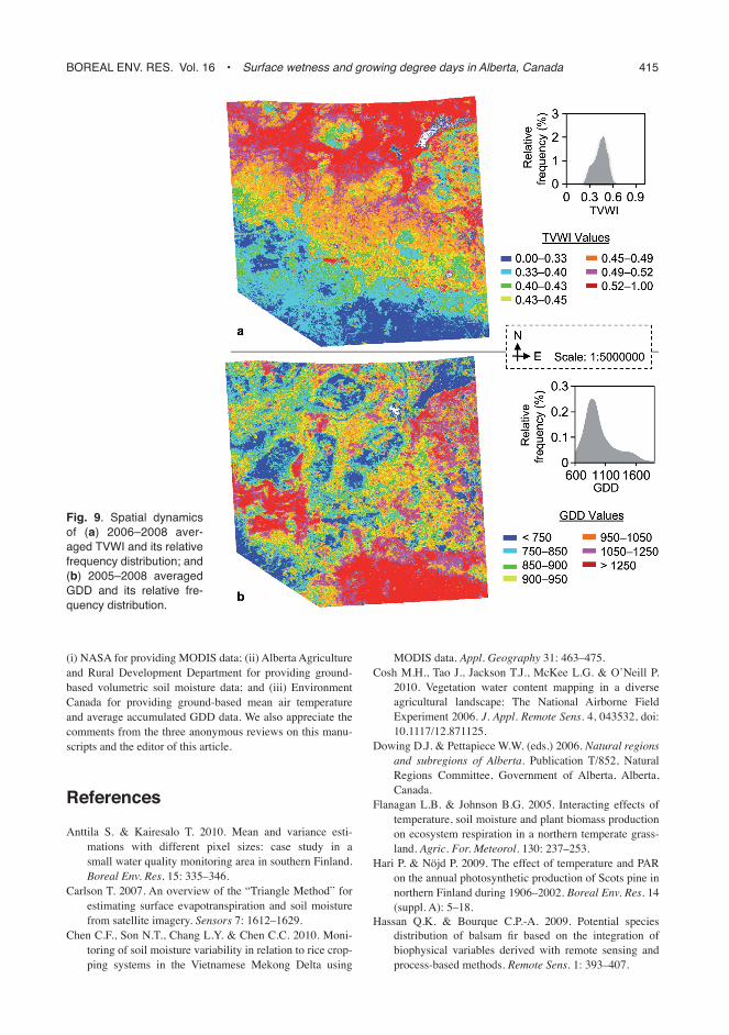
We produced the spatial distribution map of the averaged TVWI and GDD along with their respective relative frequency distributions (see Fig. 9). We found that in ~98.81% of the cases the TVWI values fell in the range of 0.2–0.6; with an average and standard deviation of ~0.44 and ~0.083, respectively (see Fig. 9a). On the other hand, we found that in ~94.89% of the cases the GDD values fell in the range of 600–1500; with an average and standard deviation of ~977 and ~250, respectively (see Fig. 9b). The distinct spatial patterns of both TVWI and GDD are summarized as follows:

260

270

280

290

300

310

320

330

0NDVI (x 10000)

Pot

entia

l sur

face

tem

pera

ture

(θs)

(K)

θdry-1 θdry-2

θwet

θdry-1 = 318, θdry-2 = –0.0035NDVI + 344.25, θwet = 275

2500 5000 7500 10000 12500

0

0.1

0.2

0.3

0.4

0.5

121

2006 2007 2008

DOY

8-da

y av

erag

ed T

VW

I and

VS

Mat

diff

eren

t dep

th o

f the

soi

l

TVWI VSM at 5 cm

153 185 217 249 121 153 185 217 249 121 153 185 217 249

VSM at 20 cm VSM at 50 cm VSM at 100 cm

Fig. 5. example of scatter plot of θs–nDvi and the corresponding dry and wet edges during the days 153–160 of the year 2006.

Fig. 6. temporal dynamics of 8-day averaged tvWi and vsm at different soil depths during the days 121–273 of the years 2006–2008.


• The higher TVWI values were found in the northern part of the study area, which might be associated with the lower GDD regimes.

• The GDD values were found to be decreasing towards the north which is associated with the gradual decrease in temperature in the same direction.

• In general, the lower TVWI values were mainly observed over agriculture-dominant areas, whereas the higher TWVI values were observed over forest-dominant regions. It might be related to the fact that dense veg-etation is able to retain water in the ground better than relatively less vegetated areas.

• We also found that higher GDD values coin-cided in the same area with relatively lower

TVWI values and vice versa. These, in par-ticular, indicate that vegetation plays a key role in regulating its surrounding climatic regimes.

• The TVWI method may be applicable in other ecosystems for assessing VSM condi-tions over topographically variable forest-dominated regions.

• The GDD method may be efficient in captur-ing GDDs in different ecosystem, however, calibration of the remote sensing data is nec-essary.

Concluding remarks

In this paper, we demonstrated the effective-ness of the TVWI approach in capturing the spatial dynamics of surface wetness conditions over agriculture and forest-dominant regions. We found that it could be used as an indirect way of determining soil moisture, because the deviation between the TVWI values and ground-based VSM were found to be within ±20% in 81.67% of the cases. In terms of GDD, we also demonstrated that our method (i.e., integration of MODIS-based Ts and ground-based Ta) was able to depict the spatial variability. We found that the relations between the MODIS-predicted and ground-based GDD values were also rea-sonably strong (i.e., within ±20% in 90.33% of the cases). Hence, it seems that remote-sensing techniques are suitable for determining these variables over other areas.

Acknowledgments: The authors would like to acknowledge partial funding support from University of Calgary to Dr. Q. Hassan. We also would like to thank the following agencies:

2007 2008

–50

–30

–10

10

30

50

121

2006

Day of year (DOY)

Dev

iatio

n (%

)

153 185 217 249121 153 185 217 249 121 153 185 217 249

700

900

1100

1300

1500

1700

700 900 1100 1300 1500 1700Ground-based average cumulated GDD

Pre

dict

ed M

OD

IS-b

ased

GD

D

n = 52

1:1 line

Deviation (%) Percentageof stations

±10±20> ±20

50.0090.399.61

Fig. 7. Deviation between the averaged ground-based measurements of vsm and tvWi for the period 2006–2008.

Fig. 8. comparison between the long-term (1971–2000) average ground-based and moDis-based aver-age (during 2005–2008) GDD values from 52 stations.


(i) NASA for providing MODIS data; (ii) Alberta Agriculture and Rural Development Department for providing ground-based volumetric soil moisture data; and (iii) Environment Canada for providing ground-based mean air temperature and average accumulated GDD data. We also appreciate the comments from the three anonymous reviews on this manu-scripts and the editor of this article.

References

Anttila S. & Kairesalo T. 2010. Mean and variance esti-mations with different pixel sizes: case study in a small water quality monitoring area in southern Finland. Boreal Env. Res. 15: 335–346.

Carlson T. 2007. An overview of the “Triangle Method” for estimating surface evapotranspiration and soil moisture from satellite imagery. Sensors 7: 1612–1629.

Chen C.F., Son N.T., Chang L.Y. & Chen C.C. 2010. Moni-toring of soil moisture variability in relation to rice crop-ping systems in the Vietnamese Mekong Delta using

MODIS data. Appl. Geography 31: 463–475.Cosh M.H., Tao J., Jackson T.J., McKee L.G. & O’Neill P.

2010. Vegetation water content mapping in a diverse agricultural landscape: The National Airborne Field Experiment 2006. J. Appl. Remote Sens. 4, 043532, doi: 10.1117/12.871125.

Dowing D.J. & Pettapiece W.W. (eds.) 2006. Natural regions and subregions of Alberta. Publication T/852, Natural Regions Committee, Government of Alberta, Alberta, Canada.

Flanagan L.B. & Johnson B.G. 2005. Interacting effects of temperature, soil moisture and plant biomass production on ecosystem respiration in a northern temperate grass-land. Agric. For. Meteorol. 130: 237–253.

Hari P. & Nöjd P. 2009. The effect of temperature and PAR on the annual photosynthetic production of Scots pine in northern Finland during 1906–2002. Boreal Env. Res. 14 (suppl. A): 5–18.

Hassan Q.K. & Bourque C.P.-A. 2009. Potential species distribution of balsam fir based on the integration of biophysical variables derived with remote sensing and process-based methods. Remote Sens. 1: 393–407.

Fig. 9. spatial dynamics of (a) 2006–2008 aver-aged tvWi and its relative frequency distribution; and (b) 2005–2008 averaged GDD and its relative fre-quency distribution.


Hassan Q.K., Bourque C.P.-A., Meng F.-R. & Richards W. 2007a. Spatial mapping of growing degree days: an application of MODIS-based surface temperatures and enhanced vegetation index. J. Appl. Remote Sens. 1, 013511, doi:10.1117/1.2740040.

Hassan Q.K., Bourque C.P.-A., Meng F.-R. & Cox R.M. 2007b. A wetness index using terrain-corrected surface temperature and normalized difference vegetation index derived from standard MODIS products: an evaluation of its use in a humid forest-dominated region of eastern Canada. Sensors 7: 2028–2048.

Hassan Q.K., Bourque C.P.-A. & Meng F.-R. 2007c. Appli-cation of Landsat-7 ETM+ and MODIS products in mapping seasonal accumulation of growing degree days at an enhanced resolution. J. Appl. Remote Sens. 1, 013539, doi: 10.1117/12.782117.

Langer M., Westermann S. & Boike J. 2010. Spatial and tem-poral variations of summer surface temperatures of wet polygonal tundra in Siberia — implications for MODIS LST based permafrost monitoring. Remote Sens. Envi-ron. 114: 2059–2069.

Latta G., Temesgen H. & Barrett T.M. 2009. Mapping and imputing potential productivity of Pacific Northwest forests using climate variables. Can. J. Forest Res. 39: 1197–1207.

Lawrence D.M., Thornton P.E., Oleson K.W. & Bonan G.B. 2007. The partitioning of evapotranspiration into transpiration, soil evaporation, and canopy evaporation in a GCM: impacts on land–atmosphere interaction. J. Hydrometrology 8: 862–880.

Li Z.L., Tang R., Wan Z., Bi Y., Zhou C., Tang B., Yan G. & Zhang X. 2009. A review of current methodologies for regional evapotranspiration estimation from remotely sensed data. Sensors 9: 3801–3853.

Moran M.S., Watts J.M., Peters-Lidard C.D. & McElroy S.A. 2004. Estimating soil moisture at the watershed scale with satellite-based radar and land surface models. Can. J. Remote Sens. 30: 805–826.

Neteler M. 2010. Estimating daily land surface temperatures in mountainous environments by reconstructed MODIS LST data. Remote Sens. 2: 333–351.

Palm C.A., Smukler S.M., Sullivan C.C., Mutuo P.K., Nyadzi G.I. & Walsh M.G. 2010. Identifying potential synergies and trade-offs for meeting food security and climate change objectives in sub-Saharan Africa. PNAS 107: 19661–19666.

Parviainen M., Luoto M. & Heikkinen R.K. 2010. NDVI-based productivity and heterogeneity as indicators of plant-species richness in boreal landscapes. Boreal Env. Res. 15: 301–318.

Patel N.R., Anapashsha R., Kumar S., Saha S.K. & Dadhwal V.K. 2009. Assessing potential of MODIS derived tem-perature/vegetation condition index (TVDI) to infer soil moisture status. Int. J. Remote Sens. 30: 23–39.

Petropoulos G., Carlson T.N. & Wooster M.J. & Islam S. 2009. A review of Ts/VI remote sensing based methods for the retrieval of land surface energy fluxes and soil surface moisture. Prog. Phys. Geography 33: 1–27.

Sandholt I., Rasmussen K. & Andersen J. 2002. A simple interpretation of the surface temperature/vegetation index space for assessment of surface moisture status. Remote Sens. Environ. 79: 213–224.

Sekhon N.S., Hassan Q.K. & Sleep R.W. 2010. Evaluating potential of MODIS-based indices in determining “snow gone” stage over forest-dominant regions. Remote Sens. 2: 1348–1363.

Shuttleworth W.J. 1988. Evaporation from Amazonian rain-forest. Proc. Roy. Soc. London B 233: 321–346.

Stenberg P., Rautiainen M., Manninen T., Voipio P. & Mottus M. 2008. Boreal forest leaf area index from optical satel-lite images: model simulations and empirical analyses using data from central Finland. Boreal Env. Res. 13: 433–443.

Su Z., Yacob A., Wen J., Roerink G., He Y., Gao B., Boog-aard H. & Diepen C.V. 2003. Assessing relative soil moisture with remote sensing data: theory, experimental validation, and application to drought monitoring over the North China Plain. Phys. Chem. Earth 28: 89–101.

Venturini V., Bisht G., Islam S. & Jiang L. 2004. Comparison of evaporative fractions estimated from AVHRR and MODIS sensors over south Florida. Remote Sens. Envi-ron. 93: 77–86.

remote sensing based estimates of surface wetness

Documents