NATIONAL CENTER FOR EARTHQUAKE ENGINEERING RESEARCH

State University of New York at Buffalo

DIGITAL SIMULATION OF

SEISMIC GROUND MOTION

by

M. Shinozuka, G. Deodatis and T. Harada Department of Civil Engineering and

Engineering Mechanics Columbia University

New York, NY 10027-6699

Technical Report NCEER-87-0017

August 31, 1987

This research was conducted at Columbia University and was partially supported by the National Science Foundation under Grant No. ECE 86-07591

NOTICE This report was prepared by Columbia University as a result of research sponsored by the National Center for Earthquake Engineering Research (NCEER). Neither NCEER, associates of NCEER, its sponsors, Columbia University, nor any person acting on their behalf:

a. makes any warranty, express or implied, with respect to the use of any information, apparatus, method, or process disclosed in this report or that such use may not infringe upon privately owned rights; or

b. assumes any liabilities of whatsoever kind with respect to the use of, or for damages resulting from the use of, any information, apparatus, method or process disclosed in this report.

50272 -101

REPORT DoCUMENTATION 11. REPORT NO.

PAGE 'NCEER-87-0017

3. Recipient's Accession No.

PS8 8 ]. 5 85 11 9 t(l lKS 4. Title and Subtitle

Digital Simulation of Seismic Ground Motion

7. Author(s)

M. Shinozuka, G. Deodatis and T. Harada 9. Performing Organization Name and Address

National Center for Earthquake Engineering Research State University of New York at Buffalo Red Jacket Quadrangle Buffalo, NY 14261

12. Sponsoring Organization' Name and Address

Same as box 9.

15. Supplementary Notes

5. Report Date

August 31, 1987 6.

S. Performing Organization Rept. No:

10. Project/Task/Work Unit No.

11. Contract(C) or Grant(G) No.

(C) [86-3043 (f(i) '''-ECE-86-07S91

13. Type of Report & Period Covered

14.

Slightly revised version of paper under same title presented at US-Japan joint seminar on Stochiastic Approaches to Earthquake Engineering, Florida Atlantic University, Boca Raton. FL. Mav 6 7. 1987. This research was C'.onouC'.ten ",1- ('",',mhi",

16. Abstract (Limit: 200 words) University and was partially supported by the National Science Foundatiol1

The method of spectral representation for uni-variate, one-dimensional, stationary stochastic processes and multi-dimensional, uni-variate (as well as multi­dimensional, mult-variate) homogeneous stochastic fields has been reviewed, particularly from the viewpoint of digitally generating their sample functions. This method of representation has then been extended to the cases of uni-variate, one-dimensional, nonstationary stochastic processes and multi-dimensional, uni-variate nonhomogeneous stochastic fields, again emphasizing sample function generation. Also, a fundamental theory of evolutionary stochastic waves is developed and a technique for digitally generating samples of such waves is intro­duced as a further extension of the spectral representation method. This is done primarily for the purpose of developing an analytical model of seismic waves that can account for their stochastic characteristics in the time and space domain. From this model, the corresponding sample seismic waves can be digitally generated. The efficacy of this new technique is demonstrated with the aid of a numerical example in which a sample of a specially two-dimensional stochastic wave consistent with the Lotung, Taiwan dense array data is digitally generated.

17. Document Analysis a. Descriptors

b. Identifiers/Open·Ended Terms

EARTHQUAKE ENGINEERING SIMULATION GROUND MOTION SPECIAL REPRESENTATION

c. COSATI Field/Group

IS. Availability Statement

Release unlimited

(See ANSI-Z39.1S)

STOCHIASTIC PROCESS POWER SPECTRUM

19. Security Class (This Report) 21. No. of Pages

I--u~n~c,-"l"-,a""s",-,=,s",i,-,,f~l~' e~d~ _____ -I __ 5¥-,--~.-,,-_____ _ 20. Security Class (This Page) 22. Price

,n,..l ",,,,c,; f'i ",,-1

See Instructions on -Reverse OPTIONAL FORM 272 (4 77) (Formerly NTIS-35) Department of Commerce

I I DIGITAL SIMULATION OF SEISMIC GROUND MOTION*

by

M. Shinozuka 1, G. Deodatis2 and T. Harada3

August 31,1987

Technical Report NCEER-87-0017

NCEER Contract Number 86-3043

NSF Master Contract Number ECE-86-07591

1 Renwick Professor, Dept. of Civil Engineering and Engineering Mechanics, Columbia University

2 Post-Doctoral Research Scientist, Dept. of Civil Engineering and Engineering Mechanics, Columbia University

3 Associate Professor, Dept. of Civil EngineeIing, Miyazaki University, Japan

NATIONAL CENTER FOR EARTHQUAKE ENGINEERING RESEARCH State University of New York at Buffalo

Red Jacket Quadrangle, Buffalo, NY 14261

* Slightly revised version of paper under same title presented at US-Japan Joint Seminar on Stochastic Approaches in Earthquake EngineeIing, Florida Atlantic University, Boca Raton, Florida, May 6-7, 1987.

SUMHARY

The method of spectral representation for uni-variate, one-dimensional,

stationary stochastic processes and multi-dimensional, uni-variate (as well as

mtilti-dimensional, multi-variate) homogeneous stochastic fields has been re­

viewed, particularly from the viewpoint of digitally generating their sample

functions. This method of representation has then been extended to the cases

of uni-variate, one-dimensional, nonstationary stochastic processes and multi­

dimensional, uni-variate nonhomogeneous stochastic fields, again emphasizing

sample function generation. Also, a fundamental theory of evolutionary sto­

chastic waves is developed and a technique for digitally generating samples of

such waves is introduced as a further extension of the spectral representation

method. This is done primarily for the purpose of developing an analytical

model of seismic waves that can account for their stochastic characteristics

in the time and space domain. From this model, the corresponding sample seis­

mic waves can be digitally generated. The efficacy of this new technique is

demonstrated with the aid of a numerical example in which a sample of a spa­

tially two-dimensional stochastic wave consistent with the Lotung, Taiwan

dense array data is digitally generated.

KEYVDRDS

Simulation; ground motion; spectral representation; stochastic pro­

cess; stochastic field; stochastic wave; stationarity; nonstationarity;

homogeneity; nonhomogeneity; power specrum; evolutionary power spectrum;

autocorrelation function.

TABLE OF CONTENTS

SECTION TITLE PAGE

1 INTRODUCTION .................................................. 1-1

2 SIMULATION OF SEISMIC GROUND MOTION USING STATIONARY PROCESS AND HOMOGENEOUS FIELD MODELS .......................... 2-1

2.1 Simulation of 1D-1V Stationary Stochastic Processes Using Spectral Representation ....................................... 2-1

2.2 Simulation of nD-1V Homogeneous Stochastic Fields Using Spectral Representation ....................................... 2-5

2.3 Simulation of nD-mV Homogeneous Stochastic Fields Using Spectral Representation ...................................... 2-10

3 SIMULATION OF SEISMIC GROUND MOTION USING NON-STATIONARY PROCESS AND NON-HOMOGENEOUS FIELD MODELS ...................... 3-1

3.1 Simulation of 1D-1V Nonstationary Stochastic Processes Using Spectral Representation ................................. 3-1

3.2 Simulation of nD-1V Nonhomogeneous Stochastic Fields Using Spectral Representation ....................................... 3-3

4 SIMULATION OF SEISMIC GROUND MOTION USING STOCHASTIC WAVES .... 4-1 4.1 Theory of nD-1V Stochastic Waves .............................. 4-1 4.2 Application to Spatially One-Dimensional Stochastic Waves ..... 4-5 4.3 Numerical Example Involving a Non-Stationary Stochastic

Wave With Two-Dimensional Spatial Nonhomogeneity .............. 4-8

5 CONCLUSION .................................................... 5-1

ACKNOWLEDGEMENT ............................................... 5 - 3

6 REFERENCES .................................................... 6-1

ii

LIST OF ILLUSTRATIONS

FIGURE TITLE PAGE

1 Function B .................................................. 4-13

2 Function W ................................................. 4-14

3 Power Spectrum f ............................................ 4-15

4a-d Simulated Stochastic Wave at 12 Equispaced Time Instants .... 4-16

5 Time History of Displacement at the Four Points A, B, C and D shown in Fig. 4a ...................................... 4-20

iii

1. INTROOOCTION

A number of stochastic models for the digital generation of artificial

ground acceleration have been proposed and successfully applied to a variety

of structural problems arising from seismic events. Referring only to repre­

sentative earlier work in this area, the following papers are cited: those by

Tajimi l , Cornel12, Housner and Jennings3, Shinozuka and Sato4, Amin and AngS,

Iyengar and Iyengar6, Ruiz and Penzien7 and Lin8• Later on, Shinozuka and his

associates introduced in a series of papers 9-14 the spectral representation

method, which can be easily implemented for the digital simulation of ground

accelerations or displacements. The papers by Shinozuka and his associates

clearly recognized the multi-variate and multi-dimensional nature of ground

motion. The most recent development in this field is the use of Auto-Regres­

sive Moving-Average (ARMA) models which have been studied by Shinozuka and his

associateslS- 19 , Spanos and his associates20- 22 and Kozin and Nakajirna23 •

A common limitation of all the above models is that ground motion is

treated as a stochastic process when its time variability is examined, or as a

stochastic field when its spatial variability is considered. In the former

case, the space variables are frozen, while in the latter case, time is fro­

zen. In order to have the analysis reflect the obvious nature of ground mo­

tion arising from a propagating seismic wave, a stochastic wave model with

evolutionary power has been developed here and an efficient technique for

digitally generating samples of such a stochastic wave is introduced as an ex­

tension of the spectral representation method primarily developed by Shinozuka

and his associates. Such a model is useful for the seismic response analysis

of such large-scale structures extending over a wide spatial area as water

transmission and gas distribution systems and large-span bridges.

1-1

2. SIMULATION OF SEISMIC GROUND MOTION USING STATIONARY PROCESS AND HOMOGENEOUS FIELD MODELS

2.1 Simulation of ID-IV Stationa Stochastic Processes Usin S ctral presentatIOn

Considerable progress has been made in stochastic modeling of ground mo-

tion and in generating the corresponding sample functions for the purpose of

nonlinear and/or parametric seismic response analyses. However, a large num-

ber of these analyses are still performed under the assumption that seismic

ground motion consists of a single horizontal component. In this respect, the

digital simulation of ID-IV (one-dimensional and uni-variate) stationary sto­

chastic processes using spectral representationl4 remains of critical impor-

tance in the seismic response analysis of structures.

Let fO(t) be a ID-IV stationary stochastic process with mean zero and

auto-correlation function Rf f (~). Then a a

E[fo(t) ] = a (1)

E[fO(t+~)fO(t) ] = Rf f (~) (2) o 0

where E[e] indicates the expectation. It is well known that Rf f (~) and the o 0

power spectral density function Sf f (w) of the process fO(t) are related o 0

through the Weiner-Khintchine transform pair:

CD •

1 J -lW~ Sf f (w) = 7it Rf f (~)e d~ o 0 -CD 0 0

CD •

J lw~ = Sf f (w)e dw -co 0 0

(3)

(4)

It follows immediately from Eg. 2 that Rf f (~) is an even function of ~, and o 0

consequently the power spectral density Sf f (w) is also an even function of o 0

w in accordance with Eq. 3. Also, it can be shown that Sf f (w) ;> O. o 0

It will be shown that the stochastic process fO(t) can be simulated by

2-1

the following series, as N ~ 00.

where

N f(t) = 12 I 12Sf f (W.)6w • cos(w.t + ¢.)

j=l 0 0 J J J

w. = j6W J

An upper round of the frequency

w = N6w u

j=1,2, ••• ,N

is implicit in Eq. 5 where w represents an upper cut-off frequency beyond u

(5)

(6)

(7)

which Sf f (w) may be assumed to be zero for either mathematical or physical o 0

reasons. In Eq. 5, ¢. are independent random phase angles uniformly distri­J

buted over the range (O,2n). Note that the simulated process is asymptoti-

cally Gaussian as N becomes large due to the central limit theorem.

It will be shown now that the expected value and auto-correlation func-

tion of the simulated process f(t) are identical to the corresponding targets,

E[fo(t)] = 0 and Rf f (~), respectively. First, utilizing the assumption that o 0

the random phase angles are independent, the expected value E[f(t)] becomes:

00 N-fold (X) N N E [f(t)] = ~ J •••••• J Y 12Sf f (W.)6W • cos(w.t+¢.)· IT [p~. (¢i)d¢i]

-00 -00 j=l 0 0 J J J i=l 1

(8)

where Pq,. (.) is the density function of tI>. and hence: 1

1

1 o " ¢. .. 2n Tn 1

PtI>. (¢i) = (9) 1

0 otherwise

2-2

The N-fold integral appearing in Eg. 8 can be written as follows:

N 00 00

= II {f Pq, (<I>. )d<l>.} J cos(w.t + <1>. )Pq, (<I>. )d<l>. i=l -00 i I I -00 J J j J J i:f:j

2n: 1 1 2 J ( ) [ . ( ,l,J' ) ] On: -- 0 = 0 "tit cos Wjt + <l>j d<P j = 2i. _sIn Wjt + 'I' (10)

It has therefore been shown that:

E[f(t)] = 0 ( 11)

Second, the auto-correlation function of the simulated process f(t) is cal-

culated as follows:

N cos [w.(t+~) + <P.] • cos [w.t + <p.]. II [p~ (<I>o)d<l>o]

I I J J ,R,=l ~~ ~ ~ (12)

The following double integral is needed in the derivation of the expression of

00 00

J J cos[w. (t+~) + <1>.] • cos[w.t + <1>.] • Pel> (<p.) • Pq, (<p. )d<l>.d<l>. = -00-00 I I J J i I j J I J

10000

='2 J J [cos{(w.+w.)t + w ... + <p. + <I>.} + -00 -00 I J I I J

+ cos{(w.-w.)t + w.'t + <I>.-<I>.}] • p~ (t!>i) • Pel> (<I>.)dt!>.d<l>. (13) I J I I J i j J I J

2-3

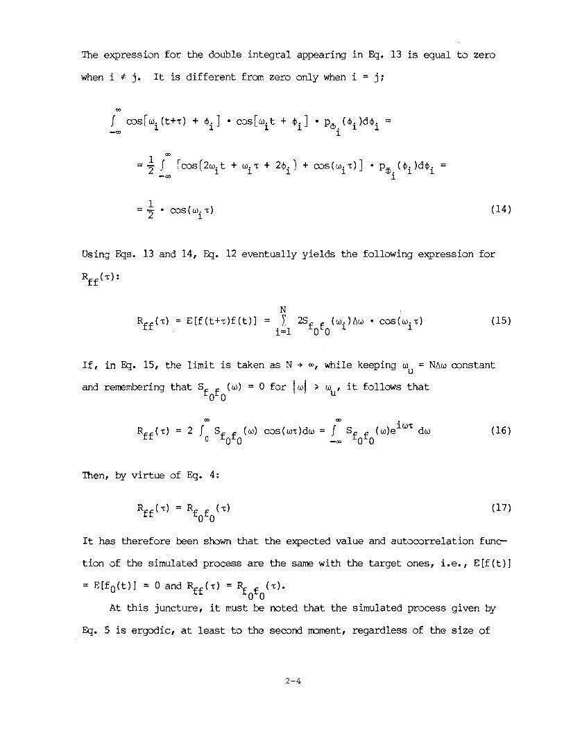
The expression for the double integral appearing in Eq. 13 is equal to zero

when i * j. It is different from zero only when i = ji

00

J ros[w.(t+'t) + ¢.] • ros[w.t + ¢.] • Pm (¢.)d¢. = 1 1 1 l'±'. 1 1

~ 1

1 00

= -2 J [ros(2w.t + W.'t + 2¢.) + ros(w.'t)] • Pm (¢. )d¢. = 1 1 1 1 ",. 1 1

-00 1

(14)

Using Eqs. 13 and 14, Eq. 12 eventually yields the following expression for

N = t 2S (w )6W • cos(w.'t)

10 ff i 1 i=l 0 0

(15)

If, in Eg. 15, the limit is taken as N ~ 00, while keeping w = N6w ronstant u

and remembering that Sf f (w) = 0 for I wi ~ wu' it follows that o 0

00 00.

J J lW't = 2 Sf f (w) cos(w't)dw = Sf f (w)e dw

o 0 0 -00 0 0 (16)

Then, by virtue of Eq. 4:

(17)

It has therefore been shown that the expected value and autororrelation func-

tion of the simulated process are the same with the target ones, i.e., E[f(t)]

= E[fO(t)] = 0 and Rff('t) = Rf f ('t). o 0

At this juncture, it must be noted that the simulated process given by

Eq. 5 is ergodic, at least to the serond moment, regardless of the size of

2-4

N 14. This makes the method directly applicable to time-domain analysis in

which the ensemble average can be evaluated in terms of the temporal average.

Finally, it should be pointed out that the computer cost of the digital gen-

eration of sample functions of process f(t) can be dramatically reduced by ap­

plying the FFT (Fast Fourier Transform) technique to Eq. 5 13.

2.2 Simulation of nD-lV Homogeneous Stochastic Fields Using _Spectral Representation

The simulation of lD-lV stationary stochastic processes using spectral

representation, which was presented in the previous section, can be extended

in a straightforward fashion to the simulation of nD-lV (n-dimensional and

uni-variate) homogeneous stochastic fields 14 in the following way.

Consider an nD-lV homogeneous stochastic field f O(xl ,x2, ••• ,xn ) = fO(~)

with mean zero:

(18)

The autocorrelation function of fO(~) is defined by

(19)

where x and x are position vectors in an n-dimensional space and _E is the -r -s

separation vector. For a homogeneous field, Rf f (~) is symmetric with res­o 0

pect to the separation vector ~ and therefore:

(20)

For some nD-lV homogeneous fields, the following equation is valid:

(21)

where I± is an nxn diagonal matrix whose diagonal components are either 1 or

2-5

- 1. Hence, Eg. 20 is a special case of Eg. 21 in which the diagonal members

of I± are all equal to - 1. When Eg. 21 is valid, the stochastic field is re­

ferred to as a "quadrant field. ,,24 AssLnTIing that an n-fold Fourier transform

of Rf f (.£) exists, the spectral density function of fO(x) is defined as: o 0

co 1 J -ik·~ Sf f '-~) = -- Rf f <.~) e - - dI o 0 (2n)n -co 0 0

and its inverse transform is given by:

co

J iK·t Rf f (~) = Sf f (K) e -- dK o 0 - -co 0 0

(22)

(23)

The preceding two equations represent the n-dimensional version of the Wiener-

Khintchine transform pair, where ~ = [Kl K2 K JT is the wave nLnTIber n

vector and ~:s. is the inner product of ~ and I, and, for simplicity:

J (24) -co

CD

Jco n-fold Jco

)dK = •••••• ()dKl dK2 ••• dKn (25) J -CD -co

It can be easily shown that:

Sf f (K) = Sf f (- K) (26) 00- 00-

and that the spectral density function is real. In addition, the'following

equation is obtained under the condition of Eg. 21:

(27)

This equation indicates that the value of Sf f (K) is identical at a corres-00-

2-6

ponding point in each quadrant (~= I± ~), hence the name "quadrant field."

Finally, it can be shown that the autocorrelation function Rf f (~) is o 0

non-negative definite and has a non-negative n-dimensional Fourier transform,

i.e. :

(28)

Based on these properties of Sf f (K), the n-dimensional homogeneous stochas-o O-

tic field fO(~) can be simulated by a stochastic field f(~) in the following

fashion: consider an nD-lV homogeneous field fO(~) with mean zero and spec­

tral density function Sf f (~) which is of insignificant magnitude outside the o 0

region defined by:

where !u = [Klu K2u

val vector by:

••••

•••

(29)

K JT with K. > 0 (i=1,2, ••• ,n). nu lU Denote the inter-

K _nu) • ••• N . (30) n

and then construct the simulated field f(~) by the following series, as Nl ,

N2, ••• ,Nn ~ m simultaneously:

N n

f(x) -r

.•.. L k =1

n

I Il=l,Ii=±1 i=2,3, ••• ,n

2-7

• • •• + (31)

where 1112 ••• 1

$ n = independent random phase angles uniformly distributed be-k1k2···kn

tween o and 21t, and

i = 1,2, ••• ,n. (32)

The simulated field f(x) is asymptotically Gaussian as N1,N2, •••• ,Nn + m si­

multaneously again due to the central limit theorem. Note that a set of II'

12, •••• , In indicates one of the 2n quadrants of the wave number! space.

Because S(!) = S(- !), we need to cover only 2n- l quadrants, half of the total

2n, for simulation purposes. Thus II is always chosen to be unity (II = 1).

This also implies that (i) there are 22n-l sets of Nl N2 ••• Nn random phase

angles in the expression for f(x) given by Eq. 31 and (ii) twice the spectral

density function always appears in the same equation.

If the stochastic field is quadrant, then SfofO(IlKlkl' 12K2k2 , •••• , InKnkn)

in Eq. 31 can be replaced by Sf f (Klk ' K2k ' •••• , Knk ). Also, if the sto-001 2 n

chastic field has a non-zero spectral density only over a pair of quadrants in

the wave number domain for which Sf f (!) = Sf f (- !), then the stochastic o 0 0 0

field is referred to as "uni-quadrant" and Eq. 31 can be written as:

N n

1. k =1

n

.... ,

•••• + Knk xn + $k k k ) n 1 2···· n

(33)

For example, a 2D-IV stochastic field is uni-~uadrant if the spectral density

is non-zero only over the first quadrant (and therefore over the third quad-

rant) •

2-8

Referring to 2D-1V homogeneous stochastic fields, Eg. 31 can be written

explicitly as

1

x cos(K1k Xl + K2k x2 + ~k(l~ ) + [28f f (K1k ,-K2k )~K1~K2]2 x 1 212 001 2

Furthermore, if the stochastic field is quadrant,

N1 N2 f(~) = 12 I J

k1 =1 k2=1

{ ( (1) ) ( (2) )} x cos K1k Xl + K2k x2 + ~ k + cos k1k Xl - K2k x2 + ~ k

1 212 1 212

(34)

(35)

(1) 1 1 (2) 1 -1 where ~ = ~' and ~ = ~' if the notation introduced in Eg. 31 is k1k2 k1k2 k1k2 k1k2

to be used. Finally, if the field is uni-quadrant over the first quadrant:

N1 N2 f(x) = 12 L 2.

kl =1 k2=1

(36)

In a way similar to the one used for the ID-IV processes, it can be shown that

the expected value and autocorrelation function of the simulated field are the

same with the target ones, i.e., E[f(~)l = E[fOCi{)l = 0 and Rff(t) = Rf f (~). o 0

Also, the nD-IV simulated field is ergodicl4 , at least to the second moment,

and the computational cost for the digital generation of sample functions of

2-9

the stochastic field f(x) can be dramatically reduced by applying the FFT

technique to the appropriate trigonometric series expression13•

2.3 Simulation of nD-rnV Homogeneous Stochastic Fields Using Spectral RepresentatiQ!2,

The simulation of nD-rnV (n-dimensional and m-variate) homogeneous stochas­

tic fields14, unlike the case of nD-IV fields, cannot be achieved by straight-

forward generalization of the ID-IV case, as shown below.

Consider a set of m homogeneous Gaussian n-dimensional stochastic fields

o f, (x) (j=1,2, ••• ,m) with mean zero: J -

(37)

and with cross-spectral density matrix ~o(~) defined by:

(38) .......................................

where S~k(K) is the n-dimensional Wiener-Khintchine transform of the cross­J -

correlation function R~k(~) (j*k) or the auto-correlation function J -

R~k (~) (j=k).

Due to the assumption of homogeneity:

o 0 R'k(l;) = R-, (- ~), J - -kJ -

the following expression can be obtained:

(39)

o -0 S 'k (K) = Sk' (K) (40)

J - J -

where the super bar indicates the rornplex ronjugate. The matrix 20 (!) is

2-10

therefore Hermitian. It can be shown that SO(~) is also non-negative definite.

SuppJse naw one can find a matrix !:!(,~) which pJssesses an n-dimensional

Fourier transform and satisfies the equation:

(41)

where ~o(~) is the specified target cross-spectral density matrix and T indi­

cates the transpJse. Then, f~ (2f) (j=1,2, ••• ,m) can be simulated by fj (x) given

below.

fj(x) (42)

where hjk(x) is the n-dimensional Fourier transform of Hjk (!):

(43)

In Eg. 42, ~(~) are independent n-dimensional Gaussian white noises such that:

(44)

with:

(45)

where 0(·) and 0 .. are the delta function and Kronecker's delta, respective-1J

lye Since ~(2f) are Gaussian, fj{x) are also Gaussian. It can be easily

verified that f.(x) (j=1,2, ••• ,m), as simulated by Eg. 42, satisfies Egs. 37 J -

and 41 and thus simulates f?(x) up to the second moments. Hence, if f?(x) is J - J -

Gaussian, f.(x) is identical with f?(x). J - J -

To find the matrix g(!) in an efficient way, we assume that H(!) is a

2-11

lower triangular matrix:

° ° ° ............. ° !!(!£) =

........................................ ..... ~ .. H (K)

rnn -

By substituting the above into Eq. 41, solutions are obtainedlO as:

k=1,2, ••• ,m

where Dk(!£) is the k-th principal minor of §O(!£) with DO being defined as

unity, and

where

sO (1,2, •••• , k-l , j) = 1,2, •••• ,k-l,k

sO 1,2, •••• ,k-l,j 1,2, •••• ,k-l,k

.....

k=1,2, ••• ,m j=k+l, ••• ,m

............................................. ° Sk-l,k-l

o S. k 1 J, -

(46)

(47)

(48)

(49)

is the determinant of a submatrix obtained by deleting all the elements except

the (1,2, ••• ,k-l,j)-th row and (1,2, ••• ,k-l,k)-th column of §O(!£). It is

noted that the above decomposition is valid only when the matrix §O(~} is Her-

mitian and positive definite as can be seen from Eq. 47.

Because the cross-spectral density matrix §O(!£} is known to be only non-

2-12

negative definite, special consideration is needed in those cases where §O(~)

has a zero principal minor14.

Once ~(~) is computed using Egs. 47 and 48, instead of passing a white

noise vector through filters, the field fj(x) can be simulated in a more effi­

cient way by the following series, as Nl ,N2, ••• ,Nn ~ 00 simultaneously and un­

der the assumption that the stochastic field possesses quadrant symmetry:

f. (x) = 2 J -

where:

i m=l

K. n IA..

I

Nl N2

Y. L ~ =1 1 .R. =1 2

•••

= ~II1K. I I

... N n L L IHjm(Kl~1'K2~2'···'Kn~n

.R. =1 Il=l,I.=±l n i=2,3,: •• ,n

K

-~) . .. -

.R. = 1,2, ••• ,N. ; I

N n

i=1,2, ••• ,n

I •

(50)

(51)

(52)

(53)

/112.' .In 'l' = independent random phase angles uniformly distributed between 0 ~1~2"'~n

and 2n. The simulated field fj(~) is asymptotically Gaussian as Nl ,N2, ••• ,Nn

~ 00 simultaneously, again due to the central limit theorem.

Finally, it can be shown again that the expected value and autocorrela-

tion function of the

ones, i.e., E [f. (x)] J -

simulated field (using Eq. 50) are

00· = E[f.(x)] = 0 and R'k(~) = R'k(~)

J- J - J-

2-13

the same as the target

j,k=1,2, ••• ,m. Al-

so, it can be shawn that the s~ulated field is ergodic14 at least to the

second moment. Here again, the computational effort for the digital genera-

tion of sample functions of the stochastic field f.(x) can be substantially J -

reduced by applying the FFT technique to Eq. 50.

2-14

3. SIMULATION OF SEISMIC GROUND MOTION USING NON-STATIONARY PROCESS AND NON-HOMOGENEOUS FIELD MODELS

3.1 Simulation of In-IV NonstationaEY Stochastic Processes Using Spectral Representation

A more realistic simulation of seismic ground motion can be made by oon-

sidering nonstationary stochastic processes or nonhomogeneous stochastic

fields. From the engineering point of view, it is highly desirable that such

non-stationary and non-homogeneous models permit physical interpretation of

their spectral contents as closely as possible to, or as a straightforward

extension of, the power spectra associated with stationary stochastic pro-

cesses or homogeneous stochastic fields. Among the various attempts to define

such non-stationary and non-homogeneous spectra, it is the "evolutionary spec­

trum" developed by Priestley25,26 that appears to offer the most palatable

transition from the power spectra associated with stationary and homogeneous

stochastic processes and fields to those associated with non-stationary and

non-homogeneous stochastic processes and fields. This is the reason why eva-

lutionary power will be used exclusively in the following.

A brief description of a In-IV nonstationary stochastic process YO(t)

with evolutionary power is given below to introduce certain notions appearing

in the theory of evolutionary power.

If a stochastic process (stationary or non-stationary) can be represented

as:

00 •

YO(t) = J A(t,w)e1wt dZ(w) (54) -00

where A(t,w) is a modulating function and dZ(w) represents an orthogonal in-

crement, the process YO(t) is said to be oscillatory. Note that the physical

3-1

notion of frequency has been preserved by including the complex exponential,

and that if A(t,w) is constant, YO(t) is a stationary process. The mean

square of the oscillatory process is found to be:

E[Y8(t)] = J IA(t,w)12 dF(w) -00

where dF(w) = E[dZ(w)]2. By introducing the evolutionary spectrum in the

form:

(55)

the non-stationary spectral contents are defined. Equation 56 may be written

as:

if f(w) exists such that dF(w) = f(w)dw, where dFO(t,w) = fO(t,w)dw. In this

case, it can also be shown that an oscillatory process YO(t) of the form of

Eq. 54 has the following auto-correlation function.

00 •

R (t+~,t) yoyo

= J A(t+~,w)A(t,w)elW~ f(w)dw (58)

It is of major importance to recognize that if the evolutionary power spectrum

can be expressed in the form of Eq. 57, then the autocorrelation function

R (t+~,t) can be calculated using Eq. 58. This is significant since it is yoyo

usually the evolutionary power spectrum of an earthquake that can be estimated

or measured and not its autocorrelation function27•

As far as the simulation procedure is concerned, the method that has been

proposed in Section 2.1 for In-IV stationary processes can be directly gen-

3-2

eralized to a non-stationary process characterized by an evolutionary power

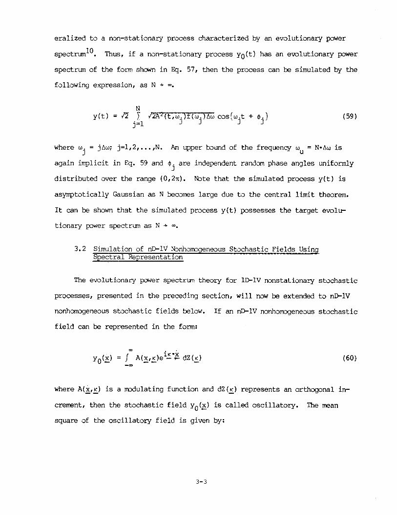
spectrumlO • Thus, if a non-stationary process YO(t) has an evolutionary power

spectrum of the form shown in Eq. 57, then the process can be simulated by the

following expression, as N + 00.

yet) N

= 12 I j=l

m 2 (t, w. ) f ( w. ) t.w cos ( w . t + 4>.) J J J J

where w. = jt.w; j=I,2, ••• ,N. An upper bound of the frequency w = N·t.w is J u

(59)

again implicit in Eq. 59 and ¢j are independent random phase angles uniformly

distributed over the range (0,2n). Note that the simulated process yet) is

asymptotically Gaussian as N becomes large due to the central limit theorem.

It can be shown that the simulated process yet) possesses the target evolu-

tionary power spectrum as N + 00.

3.2 Simulation of nO-IV Nonhomogeneous Stochastic Fields Using Spectral Representation

The evolutionary power spectrum theory for In-IV nonstationary stochastic

processes, presented in the preceding section, will naw be extended to nD-IV

nonhomogeneous stochastic fields below. If an nD-IV nonhomogeneous stochastic

field can be represented in the form:

00 . '

yO(.!) = J A(~,!.)el!..~ dZ(!.) (60) -co

where A(x,!.) is a modulating function and dZ(!.) represents an orthogonal in­

crement, then the stochastic field yO(.!) is called oscillatory. The mean

square of the oscillatory field is given by:

3-3

00

E[Y8(~)] = f IA(~,~12 dF(~) (61) -00

where

(62)

By introducing the evolutionary power spectrum of the nD-1V nonhomogeneous

stochastic field in the form:

the nonhomogeneous spectral contents are defined. Equation 63 can be written

as:

these conditions, it can be shown that an oscillatory stochastic field yO(~)

has the following autocorrelation function,

R (x+e"x) yoyo - --

00 • '

= f A(X+I,!)A(~,.!~)el~·l f(~)d!:. (65)

The stochastic field Yo(~) can be simulated in the following way, as N1,N2,

••• ,Nn + 00 simultaneously and under the assumption that the stochastic field

is quadrant symmetric:

L I 1=1,I i =±1

i=2,3, ••• ,n

•••

3-4

••• +

where:

K. n lAo

1

= ~.~K. 1 1

K' ••• Nnu)

n

~ . =1,2, ••• ,N. ; 1 1

i=1,2, ••• ,n

1112 ••• 1 ~ n = independent random phase angles uniformly distributed in the ~1~2···~n

range (O,2n).

(66)

(67)

(68)

Referring to 2D-IV nonhomogeneous stochastic fields, Eg. 66 can be writ-

ten as (quadrant symmetry is assumed):

where ~(l) ~= ~l,l and ~(2) = ~~,:l if the notation introduced in Eg. 66 is ~l ~2 ~l ~ ~l ~ Al A2

to be used. Note again that the simulated field y(~) is asymptotically Gaus-

sian as Nl,N2, ••• ,Nn + ~ simultaneously, due to the central limit theorem.

Finally, it can be shown that ~1e simulated field y(~) possesses the target

evolutionary power spectrum as Nl,N2, ••• ,Nn + ~ simultaneously.

3-5

4. SIMULATION OF SEISMIC GROUND MOTION USING STOCHASTIC WAVES

4.1 T'neory of nD-1V Stochastic Waves

An even more realistic simulation of seismic ground motion can be ob-

tained by explicitly describing it as a stochastic propagating wave. For this

purpose, consider the following spatially n-dimensional stochastic wave:

00 iK*.x* = J A(x*,~*)e - - dZ(~*) (70)

-00

where x* = [t,x1,x2

, ••• ,xnJT is an (n+1)-dimensiona1 vector containing the

time variable (t) and n space variables (x's) and ~* = [w,K1,K2, ••• ,KnJT is an

(n+1)-dimensional vector containing the frequency (w) and n wave numbers (K'S).

The frequency corresponds to the time variable, while the n wave numbers cor-

respond to the n space variables.

Note again that Eg. 70 is a direct generalization of Eg. 54 into the mul­

ti-dimensional case. Therefore, A(~*'K*) is a modulating function, dZ(~*)

represents an orthogonal increment and YO(x*) is an "oscillatory" stochastic

wave in the sense of Priestley's definition.

The mean square of the oscillatory stochastic wave is:

00

(71)

where:

(72)

Now, by introducing the (n+1)-dimensional evolutionary power spectrum in the

form:

4-1

the nonstationary and/or nonhomogeneous spectral contents are defined. Equa-

tion 73 can be written as:

(74)

if f(~*) exists such that:

(75)

It can also be shown that an oscillatory stochastic wave YO(x*) of the form

appearing in Eq. 70 has the following autocorrelation function, if Eq. 75 is

valid:

CD

R (x*+~* ,x*) yoyo - - - (76)

where the separation vector ~* is given by:

~* = [~~ ~ ••• ~ JT - 1 2 n

(77)

At this juncture, it should be pointed out that if the stochastic wave is sta-

tionary in terms of time and/or homogeneous in terms of certain space varia-

bles, then the modulating function A(x*,~*) has to be independent of the time

variable and/or these space variables, and also independent of the correspond-

ing elements of the K* vector.

The stochastic wave YO(x*) can be sllnulated in the following way as Nt,

Nl ,N2, ••• ,Nn + CD simultaneously and under the assumption that the stochastic

wave is quadrant symmetric in terms of the space variables:

4-2

y(x*) =n

where:

Nt Nl

J. y m=l i =1 1

w = mllw m

N2

I i =1 2

= ~,~KI 1 1

N n ••• I I

i =1 II =1,1. =±l n i=2,3,: •• ,n

+ ••• +

m=1,2, ••• ,Nt

i. =1,2, ••• ,N. ; 1 1

i=1,2, ••• ,n

1 11 2" •• I ~ n = independent random phase angles uniformly distributed in the mil i 2 ···.R.n

range (O,21t)

(78)

(79)

(80)

(81 )

The simulated stochastic wave y(x*) is asymptotically Gaussian as Nt,Nl'

••• ,Nn + 00 simultaneously, due to the central limit theorem. It is shawn be­

low that the autocorrelation function of the simulated stochastic wave is the

same with the target autocorrelation function R (x*+~*,x*) given by Eq. YoYO - - -

76. For this pUrp':)se, Eq. 78 is written in condensed fom as (assuming uni-

quadrant symmetry for simplicity):

N = ~ I (82)

i=l

4-3

where N = Nt NlN2oooNno The autocorrelation function of the simulated stochas-

tic wave is:

R (x*+~*,x*) = E[y(x*)y(x*+~*)J = yy--- ~--

N = E{l2 L

~=l

The expectation appearing in Ego 83 can be written as follows:

(83)

(84)

It is easy to show that the expected value shown in Eqo 84 is different from

zero only for ~=m, for which it takes the following value:

Substituting Eqo 85 into Eqo 83, the following expression is obtained for

R (x*+1;*,x*): yy- - -

N

(85)

R (x*+1;*,x*) = L 2A(X*,K*) • A(x*+1;*,K*) • f(K*) • ~K* • COS[K*·~*J (86) yy - - - - -~ - - -~ -~ -~ -~=l

In the limit as N ~ 00 and with the values of K* fixed, the preceding equation -u

becomes:

4-4

Under the assumption that the integrand in Eq. 87 is an even function of :5...*,

Eg. 87 yields:

R (x*+t:*,x*) yy - - - = J A("~_*, K*) • A(~*+~* '!.*)

-0:>

= R (x*+~*,x*) yoyo - - - (88)

4.2 Applicati6nto SpatialJ,y one-Dimensional Stochastic Waves

Having presented above the general multi-dimensional theory of stochastic

waves, a specific example is examined now, considering a spatially one-dimen-

sional stochastic wave. In this case, x* contains the time variable t and the

space variable x, i.e.:

x* = [t xJ T

and therefore the K* vector is given by:

T K* = [w K]

Then, the evolutionary power spectrum of YO(t,x) can be written as:

and the corresponding autocorrelation function as:

0:> 0:>

• e i [W't+K~] • f (w, K )dux:1K

4-5

(89)

(90)

(91)

(92)

If the stochastic wave is stationary and non-homogeneous, its evolutionary

power spectrum becomes:

(93)

and the corresponding autocorrelation function takes the form:

R ('t,x,x+1;) YOyO

<Xl <Xl

J J i [un+KF:] = A(X+t;,K) • A(X,K) • e ~. f(w,K)durlK (94)

-CD-<Xl

If the stochastic wave is homogeneous and non-stationary, its evolutionary

power spectrum becomes:

f(t,w,K)durlK = IA(t,w)12 • f(w,K)durlK (95)

and the corresponding autocorrelation function takes the form:

R (t,t+'t,1;) YoYo

<Xl <Xl

= J J A(t+'t,w) • A(t,w) • e i [w't+K1;] • f(w,K)durlK (96)

Concentrating now on the homogeneous, non-stationary stochastic wave YO(t,x),

whose spectral and correlational characteristics are described by Eqs. 95 and

96, assume that f(w,K) is in the following form in order to account for pos-

sible dispersion:

f(w,K) = f(K) • <5[w - g(K)] (97)

where <5(.} is Dirac's delta function and g(K} is a known function of K. In

this case, the simulation of the stochastic wave is performed using the fol-

lowing expression:

N y(t,x} = 12 Y. 12A[t,g(K1)]2f(K1)~K. cos[g(K1}t + K1x + ~1] (98)

1=1

4-6

It will be shown now that the autocorrelation function of the simulated sto-

chastic wave (by Eg. 98) is the same with the target autocorrelation function

given by Eg. 96.

R (t,t+T,X,X+~) = E{y(t,X)y(t+T,X+~)} = yy

N = E{12 I 12A[t,g(K~)]2. f(K~)6K • COS[g(K~)t + KXK + ~~] •

~=l

N • 12 I /2A[t+T,g(K )J2 • f(K )6K •

m=l m m

• cos [g (K ) • ( t + T) + K ( x+ ~) + ~ ]} = m m m

N N = 2 Y >' 2Art,g(K~)] • Aft+T,g(Km) ] • If(K~) • f(Km) • 6K •

~=l m=l

It can be easily shown again that the expectation appearing in Eg. 99 is dif-

ferent from zero only for ~=rn. Taking this into account, Eg. 99 becomes:

N I 2A[t,g(K~)] • A[t+T,g(K i )] • f(K~)6K • OOS[g(K~). + K~~] (100)

~=l

In the limit as N + m and with the value of K fixed, the preceding equation u

can be written as:

f 2A[t,g(K)] • A[t+T,g(K)] • f(K) • COS[g(K)T + K1;]dK o

(101)

Under the assumption that the integrand in Eg. 101 is an even function of K,

Eg. 101 yields:

4-7

R (t,t+~,x,x+~) = yy

ClO

= J A[t,g(K)] • A[t+-r,g(K)] • ei[g(Kh+K~] f(K)dK = -ClO

ClO ClO

J J i[w-r+KE] = A[t,w]· A[t+-r,w] • e • f(K) • 6[w - g(K)]dux:1K =

-CJO-<lO

ClO ClO

= J J A(t,w) • A(t+-r,w) • ei(w-r+K~) • f(K,w)dwdK =

4.3 Numerical EXample Involving a NOn-Stationary Stochastic Wave with Two-Dimensional Spatial NOnhomogeneity

(102)

The evolutionary power spectrum of a non-stationary stochastic wave with

two-dimensional spatial nonhomogeneity, is given by:

For the numerical example considered in this section, the modulating function

A(t,xl,w,Kl ) is assumed to be of the form:

(104)

B(t,w) describes the non-stationarity of the wave and is given by:

B(t w) = e61 [- O.2St] - exp[- (0.376S·w + 0.251) • t] , exp - O.2St*] - exp[- (O.376S·w + 0.251) • t*] (105)

and t* indicates the time instant at which B(t,w) assumes a maximum value as a

function of t:

4-8

t* = ~n[0.3765·w + 0.251] - ~[0.25] 0.376S·w + 0.001

The plot of B(t,w) as a function of t and w is shown in Fig. 1, whereas

W(t,Xl) describes the nonhomogeneity of the wave and is given by:

where

X = X - U ·t T B T

for Xr ( xl .;; Xr+xL

for xl > xT+xL

(106)

(107)

(108)

The following values are used for xL' xB and UT appearing in Egs. 107 and 108:

XL = 1,000 m ; XB = 6,000 m ; UT = 2,000 .....E!­sec (109)

The plot of W(t,xl) as a function of t and xl is shown in Fig. 2. The form of

f(w,Kl ,K2) is further assumed to be:

(110)

where f(Kl ,K2) is set to be:

0'2 bl Kl b2K2 f(K l ,K2) = ~ • by • b2 • Kf • exp[- (~)2 - (~)2J (Ill)

The power spectrum shown in Eg. III is proposed by Shinozuka and Harada28 and

based on data from the original accelerograrns recorded on January 29, 1981

(Event 5) by a SMART-l seismograph array installed at Lotung, Taiwan. The

data represent the horizontal component of the displacement time history in

the direction N13~1 which is approximately the direction of the seismic source

of this earthquake and are computed at each accelerograrn station from two-

4-9

component data (EW & NS). The following values are used for 0yy' bl and b2

appearing in Eq. 111:

o = 0.0124 m; yy bl

= 1131 m; b2 = 3012 m (112)

The plot of f(Kl ,K2) as a function of Kl and K2 is shown in Fig. 3. Solely for

the purpose of numerical demonstration, function g(Kl ,K2) is assumed to be of

the form:

(1l3)

in which the value of the phase velocity c is assumed to be:

c = 2,800 m/sec (114)

Finally, the stochastic wave y(t,xl,x2) can be simulated using the following

expression and under the assumption of quadrant symmetry in terms of the space

(115)

where:

(116)

(117)

4-10

(118)

The following values are used for Nl ,N2, Klu and K2u:

(119)

Klu = 8.84 x 10-3 rad/m; -3 K2u = 3.32 x 10 rad/m (120)

It is noted again that ~(l) and ~(2) are two sequences of independent random ~l~ ~1~2

phase angles uniformly distributed in the range (0,2n).

The stochastic wave is now simulated, using Eg. 115, over a 10,000 m x

10,000 m area. The simulation is performed at 12 equispaced time instants,

0.5 sec apart from each other, and shown in Fig. 4. It is clearly observed in

all twelve plots that there is relatively rapid variation along the Xl-axis

(which represents the major axis of seismic wave propagation in Event 5) com-

pared to the variation along the x2-axis. From the number of peaks (4) along

the Xl-axis, the apparent wave length along this axis is estimated to be

around 2,500 m. Thus, the patterns shown in Fig. 4 indicate a dominant wave

with a wave length of approximately 2,500 m propagating in the negative xl­

direction. By dividing the distance covered by a single peak (5,500 m) by the

elapsed time (2.0 sec), the approximate speed of wave propagation along the

Xl-axis is estimated to be 2,750 m/sec. This value is practically identical

to the value of 2,800 m/sec specified in Eq. 114. These wave length and phase

velocity values result in a dominant frequency of approximately 2,800/2500 •

1.12 Hz. This is also confirmed by Fig. 5 which plots the time history of the

displacement at Xl = 3,500 m and x2 = 1,000 m (point A in Fig. 4a). The ap­

parent frequency observed in this plot is 1/0.75 sec = 1.33 Hz, which is very

close to the above-mentioned dominant frequency of 1.12 Hz. The time histo-

ries at points B, C and D (also shown in Fig. 4a) are also plotted in Fig.

4-11

5. The time histories at A, B and C show the spatial variability along the

major axis of wave propagation while those at A and D along the direction

perpendicular to that. The propagating wave front is clearly seen in Fig. 4b

as well as in the first three frames of Fig. 5 (points A, B and C). The

ground is at rest in front of the wave front because of Eg. 107. Another in­

teresting feature that can be observed in Fig. 4 is the initial gradual in­

crease of the amplitude of the wave and the subsequent gradual decrease which

is an actual feature of all strong ground motions. At this point, it is

pointed out that the same procedure as the one described above for the digital

simulation of the displacement time history can be used for the digital simu­

lation of either the velocity or acceleration time history, by properly choos­

ing the corresponding evolutionary power spectra.

Finally, it is noted that the CPU time necessary to generate 2lx2l points

at a specific time instant was approximately 11 minutes (on a SUN 3/180 com­

puter system).

4-12

o

6 r:ad/sec

Fig. 1 Function B(t,w).

4-13

10 sec

Fig. 2 Fuuction 1V(t,xd·

4-14

o

0.005 rad/sec

Fig. 3 power Spectrum f(hl, h2)'

4-15

Fig. 4a Simulated Stochastic Wave at 12 Equispaced Time Instants (con­figuration of simulated points).

4-16

Fig. 4b

4-17

t = 2.5sec t = 3.0sec

t = 3.5sec t = 4.0sec

Fig. 4c Simulated Stochastic Wave at 12 Equispaced Time Instants.

4-18

t = 4.5sec t = 5.0sec

t = 5.5sec t = 6.0sec

Fig. 4d Simulated Stochastic Wave at 12 Equispaced Time Instants.

4-19

.01

.03 Point A

....--.- .02

a

.IK

.03

....--.- .02

a ~

~ .01 .::: Q.)

a 0 Q.)

u C';l -a -.01

rn ......

Point B

Q -.02 Q -.02

-.03

-.04 ~,-,-,=,.u...,-!-,-LU::~~"'!-':~~~~~"'7'~:-t:-~~~ o .5 1.0 1.5 2.0 2.5 !.O !.S 4.0 4.5 S.O S.S 8.0

Time (sec)

.03 Point C

.02

.01

-.01

-.02

-.03

-.IK O .5 1.0 1.5 2.0 2.5 3.0 3.5 1.0 1.5 5.0 5.5 6.0

Time (sec)

-.O~

-.~ 0 .S 1.0 I.S t.O 2.S '.0 '.5 1.0 1.S S.O S.S '.0

.03

.---... .02 a ~

~ .DI

Q.)

~ 01----..... U

~ 0.. -.01 rn ......

-.G2

Time (sec)

Point D

-.1It u....u..l.1.u...J..u.u.u~"O"'U" ........ u...u ........ .I.I..L ........ u...u-LU..l.l..Lu...uu..u.L.U.LJ o .5 1.0 1.5 2.0 2.5 '.0 '.5 1.0 1.5 5.0 5.5 8.0

Time (sec)

Fig. 5 Time History of Displacement at the Four Points A, B, C and D shown in Fig. 4a.

4-20

5. CONCLUSION

This paper presented fundamentals of the theory of multi-dimensional and

multi-variate stochastic fields and stochastic waves. This was done primarily

from the viewpoint of applying it to the digital generation of seismic ground

motion for the purpose of seismic response analysis of lifeline systems

extending over a large spatial area. The method appears to work very well, as

exemplified by a numerical example where a propagating seismic wave idealized

as a spatially two-dimensional stochastic wave is digitally generated.

While such results are gratifying, there appear to be some issues that

still need to be resolved by future study. For example, the spectral repre­

sentation used in this paper produces mathematical models for stochastic pro­

cesses, fields and waves which are asymptotically Gaussian. However, Gaus­

sianess may not always apply to the actual ground motion data. If the data

exhibit some deviation from Gaussianess, and such deviation is expected to

substantially affect the result of the ensuing analysis, then non-Gaussian

characteristics must be introduced into the model. In this respect, a recent

work by Yamazaki and Shinozuka29 may prove to be quite useful, because the

paper29 deals with multi-dimensional stochastic fields and introduces non­

Gaussian characteristics still on the basis of spectral representation. An

alternative consists of the use of shot noise or filtered Poisson process

models, as demonstrated by Lin8 and Shinozuka and Sato4• More recently, Lin30

showed how the evolutionary power spectrum can be incorporated into the fil­

tered Poisson model. However, these filtered Poisson models are limited to

one-dimensional and uni-variate cases at this time.

Another issue that requires further study is the question of how more

general dispersion characteristics can be incorporated into the model. In the

present formulation, a particular relationship is assumed for the frequency

5-1

and wave numbers. In this connection, if a number of seismic waves of specif­

ic characteristics are known to be propagating simultaneously, the spectral

representation of these models can be constructed individually and summed up

vectorially to develop a simulation of such a composite wave. Since, however,

the observed ground motion is a composite of seismic waves with various char­

acteristics, no simple relationship can really be assigned to the frequency

and wave number. It is therefore reasonable to assume that a multiplicity of

such relationships exist in reality and, indeed, the power spectral density

obtained from ground motion data involving the frequency and all pertinent

wave numbers should contain information relevant to this. It is important and

also interesting to pursue this issue. It should be noted that Scherer and

Schueller have done some interesting work in this area31•

Another aspect of future work is the extension of the introduced simula­

tion technique to multi-variate non-stationary and/or nonhomogeneous cases of

stochastic waves. However, such a task might be particularly difficult, be­

cause the cross-correlational characteristics of such waves are usually very

complicated and no reliable data are available at this time for non-stationary

and/or nonhomogeneous multi-variate stochastic waves.

The simUlation of ground motion described in this paper represents, in

essence, mathematically tractable and physically meaningful models. Indeed,

we have come a long way from the early mathematical model in which a Gaussian

white noise is passed through an appropriate filter by means of a convolution

integral to produce In-IV artificial ground accelerations. While some attempt

has been made in this paper to incorporate into the models the physical laws

of propagating seismic waves, further efforts should be directed to the im­

provement of these models so as to reflect the physics of seismic waves in­

cluding their source mechanism, attenuation, etc.

5-2

Finally, the following problem is currently under investigation: given

the evolutionary power spectrum of a spatially two-dimensional, nonhomogene­

ous, non-stationary stochastic wave (shown in Eg. 103), derive the corres­

ponding evolutionary power spectrum of the non-stationary stochastic process

obtained by freezing the space variables Xl and x2 at a specific point. Clar­

ification of the above issue will provide further insight into the theory of

stochastic waves.

ACKNa-vLED3EMENT

This work was supported by Sub-contract No. SUNYRF-NCEER-86-3043 under

the auspices of the National Center for Earthquake Engineering Research under

NSF Grant No. ECE-86-0759l.

5-3

REFERENCES

1. Tajimi, H., "Basic Theories on Aseismic Design of Structures," Institute of Industrial Science, University of Tokyo, Vol. 8, No.4, March 1959.

2. Cornell, C.A., "Stochastic Process MJdels in Structural Engineering," Technical Report No. 34, Dept. of Civil Engineering, Stanford University, May 1960.

3. Housner, G.W. and Jennings, P.C., "Generation of Artificial Earthquakes," Journal of Engineering Mechanics, ASCE, Vol. 90, No. EMI, February 1964, pp. in-Iso.

4. Shinozuka, M. and Sato, Y., "Simulation of Nonstationary Random Process," Journal of Engineering Mechanics ASCE, Vol. 93, No. EMl, February 1967, pp. 11-40.

5. Amin, M. and Ang, A.H-S., "Nonstationary Stochastic MJdels of Earth­quake," Journal of Engineering Mechanics, ASCE, Vol. 94, No. EM2, April 1968, pp. 559-583.

6. Iyengar, R.N. and Iyengar, K.T.S., "A N::mstationary Random Process l>bdel for Earthquake Accelerograrns," BUlletin of the Seismoiogical Society of America, Vol. 59, No.3, June 19b9, pp. 1163-1188.

7. Ruiz, P. and Penzien, J., "Stochastic Seismic Response of Structures," Journal of Engineering Mechanics, ASCE, Vol. 97, No. EM2, April 1971, pp. 441-456.

8. Lin, Y-K., "Nonstationary Excitation and Response Treated as Sequences of Random Pulses," i!::)urnal of the Acoustical Society of America, Vol. 38, 1965, pp. 453-460.

9. Shinozuka, M., "Monte Carlo Solution of Structural Dynamics," lnterna­tional J:)urnal of Computers and Structures, Vol. 2, 1972, pp. 855-874.

10. Shinozuka, M. and Jan, C-M., "Digital Simulation of Random Processes and Its Applications," Journal of Sound and Vibration, Vol. 25, N::>. 1, 1972, pp. 111-128.

11. Iyengar, R.N. and Shinozuka, M., "Effect of Self-Weight and Vertical Ac­celeration on the Behavior of Tall Structures During Earthquake," Journal of Earthquake Engineering and Structural pynamics, Vol. 1, 1972, pp. 69-78.

12. Shinozuka, M., "Digital Simulation of Ground Acceleration," Proceedings of the 5th W:)rld Conference on Earthquake Engineering, Rome, Italy, June 1973, pp. 2829-2838.

13. Shinozuka, M., "Digital Simulation of Random Processes in Engineering Mechanics with the Aid of FIT Technique," Stochastic Problems in Mechan­ics, Eds. S.T. Ariaratnam ane H.H.E. Leipholz, (Waterloo: University of ~erloo Press), 1974, pp. 277-286.

6-1

14. Shinozuka, M., "Stochastic Fields and Their Digital Simulation," Lecture Notes for the CISM Course on Stochastic Methods in Structural Mechanics, Udine, Italy, August 28-30, 1985.

15. Samaras, E.F., Shinozuka, M. and Tsurui, A., "ARMA Representation of Ran­dom Vector Processes," Journal of Engineering Mechanics, ASCE, Vol. 111, No.3, pp.449-46l.

16. Naganurna, T. et al., "Digital Generation of Multidimensional Random Fields," Proceedings of ICOSSAR '85, Kobe, Japan, May 27-29, 1985, pp. 1. 251 - r-:2bo.

17. Naganuma, T., Deodatis, G. and Shinozuka, M., "ARMA Model for Two-Dimen­sional Processes," Journal of Engineering Mechanics, ASCE, Vol. 113, No. 2, February 1987, pp. 234-251.

18. Deodatis, G., Shinozuka, M. and Samaras, E., "An AR Model for Non-Sta­tionary Processes," Proceedings of the 2nd International Conference on Soil Dynamics and Earthquake Engineering, on board the liner Queen Elizabeth 2, New York to Southampton, June/July 1985, pp. 2.57 - 2.66.

19. Deodatis, G. and Shinozuka, M., "An Auto-Regressive Model for Non-Sta­tionary Stochastic Processes," accepted for publication in the ASCE Journal of Engineering Mechanics.

20. Spanos, P.D. and Hansen, J., "Linear Prediction Theory for Digital SUnu­lations of Sea Waves," Journal of Energy Resources Technology, ASME, Vol. 103, 1981, pp. 243-249.

21. Spanos, P.D., "ARMA Algorithms for O::ean Spectral M:>deling," Journal of Energy Resources Technology, Vol. 105, 1983, pp. 300-309.

22. Spanos, P.D. and Solorros, G.P., "Markov Approximation to Nonstationary Random Vibration," Journal of Engineering ~1echanics, ASCE, Vol. 109, No. 4, 1983, pp. 1134-1130.

23. Kozin, F. and Nakajima, F., "The Order Determination Problem for Linear Time-Varying AR Models," IEEE Transactions on Automatic Control, Vol. AC-25, No.2, 1980, pp. 250-257.

24. Vanrnarcke, E., Random Fields, (Cambridge: MIT Press), 1984.

25. Priestley, M.B., "Evolutionary Spectra and Non-Stationary Processes," Journal of the Royal Statistical Socie~ Series B., Vol. 27, 1965, pp. 204-237.

26. Priestley, M.B., "Power Spectral Analysis of Non-Stationary Random Pro­cesses," Journal of Sound and Vibratio!:!., Vol. 6, No.1, 1967, pp. 86-97.

27. Liu, S-C., "Evolutionary Power Spectral Density of Strong M:>tion Earth­quakes," Bulletin of the Seisrrological Society of America, Vol. 60, No. 3, 1970, pp. 891-900.

28. Shinozuka, M. and Harada, T., "Harmonic Analysis and Simulation of Homo-

6-2

geneous Stochastic Fields," Technical Report, ~partment of Civil Engin­eering and Engineering Mechanics, Columbia University, New York, 1986.

29. Yamazaki, F. and Shinozuka, M., "Digital Generation of NOn-Gaussian Sto­chastic Fields," Technical Report, ~partrnent of Civil Engineering and Engineering l'-1echanics, Columbia University, New York, 1986.

30. Lin, Y-K., "On Random Pulse Train and Its Evolutionary Spectral Repre­sentation," Journal of Probabilistic Engineering Mechanics, Vol. 1, NO. 4, ~cember 1986, pp. 219-223.

31. Scherer, R.J. and Schueller, G.I., "The Acceleration Spectrum at the Base Rock ~termined From a Non-Stationary Stochastic Source Model," Proceed­

of the 8th Euro an Conference on Earth uake En ineerin , Portugal,

6-3