digital image processing of remotely sensed … · digital image processing of remotely sensed...
TRANSCRIPT

DIGITAL IMAGE PROCESSING OF REMOTELY SENSED
OCEANOGRAPHIC DATA
MUSERREF TURKMEN
AUGUST 2008
DIGITAL IMAGE PROCESSING OF REMOTELY SENSED
OCEANOGRAPHIC DATA
A THESIS SUBMITTED TO
THE GRADUATE SCHOOL OF APPLIED MATHEMATICS
OF
THE MIDDLE EAST TECHNICAL UNIVERSITY
BY
MUSERREF TURKMEN
IN PARTIAL FULFILLMENT OF THE REQUIREMENTS FOR THE
DEGREE OF
MASTER OF SCIENCE
IN
THE DEPARTMENT OF SCIENTIFIC COMPUTING
AUGUST 2008

Approval of the Graduate School of Applied Mathematics
Prof. Dr. Ersan AKYILDIZ
Director
I certify that this thesis satisfies all the requirements as a thesis for the degree of
Master of Science.
Prof. Dr. Bulent KARASOZEN
Head of Department
This is to certify that we have read this thesis and that in our opinion it is fully
adequate, in scope and quality, as a thesis for the degree of Master of Science.
Assist. Prof. Dr. Hakan OKTEM Prof. Dr. Bulent KARASOZEN
Supervisor Co-supervisor
Examining Committee Members
Assoc. Prof. Dr. Azize HAYFAVI
Assist. Prof. Dr. Hakan OKTEM
Prof. Dr. Gerhard Wilhelm WEBER
Assoc. Prof. Dr. Emrah CAKCAK
Assist. Prof. Dr Fahd JARAD

I hereby declare that all information in this document has been ob-
tained and presented in accordance with academic rules and ethical
conduct. I also declare that, as required by these rules and conduct,
I have fully cited and referenced all material and results that are not
original to this work.
Name, Last name: Muserref TURKMEN
Signature:
iii

abstract
DIGITAL IMAGE PROCESSING OF REMOTELY
SENSED OCEANOGRAPHIC DATA
TURKMEN, Muserref
M.Sc., Department of Scientific Computing
Supervisor: Assist. Prof. Dr. Hakan OKTEM
Co-supervisor: Prof. Dr. Bulent KARASOZEN
August 2008, 106 pages
Developing remote sensing instrumentation allows obtaining information about
an area rapidly and with low costs. This fact offers a challenge to remote sensing
algorithms aimed at extracting information about an area from the available re-
mote sensing data. A very typical and important problem being interpretation of
satellite images. A very efficient approach to remote sensing is employing discrim-
inant functions to distinguish different landscape classes from satellite images.
Various methods on this direction are already studied. However, the efficiency
of the studied methods are still not very high. In this thesis, we will improve
efficiency of remote sensing algorithms. Besides we will investigate improving
boundary detection methods on satellite images.
Keywords: remote sensing, sea surface temperature, image processing, mathe-
matical morphology, edge detection, segmentation, reconstruction.
iv
OZ
UZAKTAN ALGILANAN OKYANUS VERILERINDE
SAYISAL GORUNTU ISLEME
TURKMEN, Muserref
Yuksek Lisans, Bilimsel Hesaplama Bolumu
Tez Danısmanı: Assist. Prof. Dr. Hakan OKTEM
Tez Yardımcısı: Prof. Dr. Bulent KARASOZEN
Agustos 2008, 106 sayfa
Uzaktan Algılama aracları gelistirmek daha az maliyetle daha hızlı bilgi edin-
memize olanak tanır. Bu nedenle gelistirilmis uzaktan algılama algoritmaları kul-
lanılabilir uzaktan algılama verileri sayesinde bilgi edinmeyi daha kolaylastırmayı
amaclar. Uydu goruntulerini yorumlamak onemli bir problemdir. Uzaktan algı
lamada diskriminant fonksiyonlarını kullanarak uydu goruntulerinden degisik alan-
ları ayırt etmek cok etkili bir yontemdir. Bu yondeki cesitli metotlar arastırılmıstır.
Ancak calısılan yontemlerin performansı hala cok yuksek degildir. Bu tezde,
uzaktan algılama metotlarının performansını artıracagız. Ayrıca sınırlı algılama
algoritmalarının gelistirilmesini arastıracagız.
Anahtar Kelimeler: uzaktan algılama, deniz yuzeyi sıcaklıgı, goruntu isleme,
matematiksel morfoloji, sınır bulma, kesimleme, yeniden yapılandırma.
v

To my parents
vi

ACKNOWLEDGEMENTS
I do not have enough words to express how thankful I am to my advisor Assist.
Prof. Dr. Hakan Oktem for his supervision, advice, patiently guiding, motivating
and especially the encouragement he has given me throughout this study.
I am thankful to my co-supervisor Prof. Dr. Bulent Karasozen for his kindness
and suggestions throughout this study.
I am grateful to my inspiration Mustafa Duzer for gathering all the data used
in this thesis, always being by my side and supporting me during this long process.
I want to thank my dear friend Hatice who offered her help and support contin-
uously me since the first day of this project.
I also want to thank my dear friends Mustafa, Onder, Derya, Nurgul and Nilufer
for their endless support and being with me all the time.
I thank the members of IAM for all their constructive comments and their sup-
port.
I am grateful the member of IMS especially Murat, Serkan and Hasan for intro-
ducing me to atmospheric science and oceanography and making research in this
field seem so exciting. They offered me so generously a perfect working environ-
ment, support, and help whenever I needed it. I feel so lucky for just having the
opportunity to work with them and learn from them, during my studies.
vii

Finally I would like to thank my dear family for always being by my side, for
their understanding and patient dispositions, and their endless support. Without
them this thesis would have never been written.
viii

table of contents
PLAGIARISM . . . . . . . . . . . . . . . . . . . . . . . . . . . . . . . . . . . . . . . . . . . . . iii
ABSTRACT . . . . . . . . . . . . . . . . . . . . . . . . . . . . . . . . . . . . . . . . . . . . . . . iv
OZ . . . . . . . . . . . . . . . . . . . . . . . . . . . . . . . . . . . . . . . . . . . . . . . . . . . . . . . . . . v
DEDICATION . . . . . . . . . . . . . . . . . . . . . . . . . . . . . . . . . . . . . . . . . . . . . vi
ACKNOWLEDGEMENTS . . . . . . . . . . . . . . . . . . . . . . . . . . . . . . . . vii
TABLE OF CONTENTS . . . . . . . . . . . . . . . . . . . . . . . . . . . . . . . . . ix
LIST OF FIGURES . . . . . . . . . . . . . . . . . . . . . . . . . . . . . . . . . . . . . . . xiii
LIST OF TABLES . . . . . . . . . . . . . . . . . . . . . . . . . . . . . . . . . . . . . . . . . xv
CHAPTER
1 INTRODUCTION . . . . . . . . . . . . . . . . . . . . . . . . . . . . . . . . . . . . . . 1
1.1 Objectives . . . . . . . . . . . . . . . . . . . . . . . . . . . . . . . 1
1.2 Thesis Outline . . . . . . . . . . . . . . . . . . . . . . . . . . . . . 2
ix

2 THEORETICAL BACKGROUND . . . . . . . . . . . . . . . . . . . . 4
2.1 Introduction to Remote Sensing . . . . . . . . . . . . . . . . . . . 4
2.2 Introduction to Satellites . . . . . . . . . . . . . . . . . . . . . . . 9
2.2.1 NOAA-AVHRR . . . . . . . . . . . . . . . . . . . . . . . . 11
2.2.2 NIMBUS . . . . . . . . . . . . . . . . . . . . . . . . . . . 11
2.2.3 Metosat . . . . . . . . . . . . . . . . . . . . . . . . . . . . 12
2.2.4 LANDSAT . . . . . . . . . . . . . . . . . . . . . . . . . . 13
2.2.5 IKONOS . . . . . . . . . . . . . . . . . . . . . . . . . . . . 14
2.2.6 CZCS . . . . . . . . . . . . . . . . . . . . . . . . . . . . . 14
2.3 MODIS (Moderate Resolution Imaging Spectroradiometer) . . . 15
2.3.1 Preprocessing of Data . . . . . . . . . . . . . . . . . . . . 16
2.3.2 Overview of MODIS Aqua Data Processing and Distribution 20
2.3.3 Implementation of SST Processing . . . . . . . . . . . . . 24
2.3.4 MODIS ocean data processing codes . . . . . . . . . . . . 26
3 MATHEMATICAL BACKGROUND . . . . . . . . . . . . . . . . . . 29
3.1 Introduction to Vectors and Matrices . . . . . . . . . . . . . . . . 29
3.1.1 Matrices and Two-dimensional Arrays . . . . . . . . . . . 31
3.1.2 Properties of Vectors and Matrices . . . . . . . . . . . . . 32
3.1.3 Solutions to Systems of Linear Equations . . . . . . . . . . 34
3.1.4 Singular Value Matrix Decomposition (SVD) . . . . . . . . 36
3.2 Interpolation and Curve Fitting . . . . . . . . . . . . . . . . . . . 37
x

3.2.1 Lagrange Interpolation . . . . . . . . . . . . . . . . . . . . 38
3.2.2 Newton Interpolation . . . . . . . . . . . . . . . . . . . . . 39
3.2.3 Spline Interpolation . . . . . . . . . . . . . . . . . . . . . . 40
3.3 Mathematical Morphology . . . . . . . . . . . . . . . . . . . . . . 41
3.3.1 Dilation . . . . . . . . . . . . . . . . . . . . . . . . . . . . 42
3.3.2 Erosion . . . . . . . . . . . . . . . . . . . . . . . . . . . . 43
3.3.3 Opening and closing . . . . . . . . . . . . . . . . . . . . . 43
4 INTRODUCTION TO IMAGE PROCESSING . . . . . . 45
4.1 Edge Detection . . . . . . . . . . . . . . . . . . . . . . . . . . . . 45
4.2 Segmentation . . . . . . . . . . . . . . . . . . . . . . . . . . . . . 53
4.2.1 Pixel Based Segmentation . . . . . . . . . . . . . . . . . . 53
4.2.2 Edge Based Segmentation . . . . . . . . . . . . . . . . . . 54
4.2.3 Region Based Segmentation . . . . . . . . . . . . . . . . . 56
4.3 Reconstruction . . . . . . . . . . . . . . . . . . . . . . . . . . . . 60
4.3.1 Propagation . . . . . . . . . . . . . . . . . . . . . . . . . . 60
4.3.2 Morphological Reconstruction . . . . . . . . . . . . . . . . 61
5 METHODS . . . . . . . . . . . . . . . . . . . . . . . . . . . . . . . . . . . . . . . . . . . . . . 62
5.1 Data Preparation . . . . . . . . . . . . . . . . . . . . . . . . . . . 62
5.2 Preprocessing . . . . . . . . . . . . . . . . . . . . . . . . . . . . . 63
5.3 Interpolation . . . . . . . . . . . . . . . . . . . . . . . . . . . . . 63
5.3.1 Spline Interpolation . . . . . . . . . . . . . . . . . . . . . . 64
xi

5.3.2 Minimum Mean-Square Error Curve Fitting . . . . . . . . 69
5.4 Edge Detection . . . . . . . . . . . . . . . . . . . . . . . . . . . . 74
5.4.1 Canny Edge Detector . . . . . . . . . . . . . . . . . . . . . 75
5.5 Segmentation . . . . . . . . . . . . . . . . . . . . . . . . . . . . . 79
5.5.1 Watershed Segmentation . . . . . . . . . . . . . . . . . . . 79
5.5.2 Results . . . . . . . . . . . . . . . . . . . . . . . . . . . . . 80
5.6 Reconstruction . . . . . . . . . . . . . . . . . . . . . . . . . . . . 81
6 CONCLUSIONS AND FUTURE WORK . . . . . . . . . . . . . 87
6.1 Conclusions . . . . . . . . . . . . . . . . . . . . . . . . . . . . . . 87
6.2 Future Work . . . . . . . . . . . . . . . . . . . . . . . . . . . . . . 97
REFERENCES . . . . . . . . . . . . . . . . . . . . . . . . . . . . . . . . . . . . . . . . . . . . 101
APPENDICES . . . . . . . . . . . . . . . . . . . . . . . . . . . . . . . . . . . . . . . . . . . . . 107
Appendix A . . . . . . . . . . . . . . . . . . . . . . . . . . . . . . . . . 107
MATLAB Code for Conversion of HDF . . . . . . . . . . . . . . . 107
MATLAB Code for Histogram Modification . . . . . . . . . . . . 111
MATLAB Code for Reconstruction . . . . . . . . . . . . . . . . . 116
Appendix B . . . . . . . . . . . . . . . . . . . . . . . . . . . . . . . . . 122
xii
list of figures
2.1 Remote sensing system. . . . . . . . . . . . . . . . . . . . . . . . 5
2.2 Satellite orbit and swath. . . . . . . . . . . . . . . . . . . . . . . . 10
2.3 Level-2 processing. . . . . . . . . . . . . . . . . . . . . . . . . . . 23
5.1 The cubic polynomial f(x) = (x−1)(x−2)(x−3), and its piecewise
linear interpolant (dashed line) at the nodes xk = x0+hk for which
x0 = 0, and h = 12, where k = 0, 1, . . . , n with n = 8. . . . . . . . . 65
5.2 Natural and complete (respectively) spline interpolants (dashed
lines) for the function f(x) = e−x2(solid lines) on the interval
[−1, 1]. The circles correspond to node locations. Here n = 4,
with h = 12 , and x0 = −1. The nodes are at xk = x0 + hk for
k = 0, . . . , n. . . . . . . . . . . . . . . . . . . . . . . . . . . . . . 67
5.3 A linear estimate . . . . . . . . . . . . . . . . . . . . . . . . . . . 71
5.4 The least squares parabola for the points (−3, 3), (0, 1), (2, 1), and
(4, 3). . . . . . . . . . . . . . . . . . . . . . . . . . . . . . . . . . . 75
5.5 SST image . . . . . . . . . . . . . . . . . . . . . . . . . . . . . . . 77
5.6 Sobel method . . . . . . . . . . . . . . . . . . . . . . . . . . . . . 78
5.7 Canny method . . . . . . . . . . . . . . . . . . . . . . . . . . . . 78
5.8 Combination of Canny and Edge Tracing Method . . . . . . . . . 79
5.9 Controlled Watershed Segmentation Method . . . . . . . . . . . . 82
5.10 Filtered and Traced image . . . . . . . . . . . . . . . . . . . . . . 82
5.11 Incomplete image . . . . . . . . . . . . . . . . . . . . . . . . . . . 85
xiii

5.12 Fitting image . . . . . . . . . . . . . . . . . . . . . . . . . . . . . 85
5.13 Interpolation of missing data . . . . . . . . . . . . . . . . . . . . . 86
5.14 Better reconstruction . . . . . . . . . . . . . . . . . . . . . . . . . 86
6.1 Before Adaptive Histogram Modification algorithm. . . . . . . . . 88
6.2 After Adaptive Histogram Modification algorithm. . . . . . . . . . 90
6.3 Raw SST image. . . . . . . . . . . . . . . . . . . . . . . . . . . . 91
6.4 After deleting incorrect pixels. . . . . . . . . . . . . . . . . . . . . 92
6.5 After image to map projection our image is more understandable. 93
6.6 Reconstructed data. . . . . . . . . . . . . . . . . . . . . . . . . . . 95
6.7 Segmentation is done. . . . . . . . . . . . . . . . . . . . . . . . . . 96
6.8 Another SST image before reconstruction end segmentation. . . . 99
6.9 After image processing. . . . . . . . . . . . . . . . . . . . . . . . . 100
xiv

list of tables
2.1 Coefficients and residual SST errors of linear single band atmo-
spheric correction algorithm [Atbd-mod25]. . . . . . . . . . . . . . 20
4.1 Gradient edge detector masks. . . . . . . . . . . . . . . . . . . . . 48
4.2 Masks for Edge Detection [18] . . . . . . . . . . . . . . . . . . . . 51
xv

chapter 1
INTRODUCTION
1.1 Objectives
Remote sensing and other satellite measurements in recent years have pro-
vided meteorologists, oceanographers and geodesists with new techniques for ob-
servations. The accuracy of satellite observations of the ocean surface is the
reason we choice satellite derived data, i.e., Spatial resolution = 1km.
One of the most important contributions of satellite remote sensing to climate
studies is the establishment of global sea surface temperature (SST) data sets.
One use of regular global SST data is to test estimates of global warming due to
increases in atmospheric carbon dioxide. Another use of SST data sets is to detect
SST anomalies, which are associated with changes in atmospheric circulation and
hence the weather. In addition to them SST data have many use in oceanography
and more proper data give more suitable result. Namely, if we are able to improve
the efficiency of processing techniques we can provide more accurate data so one
can get better result of usage of SST.
In this thesis we aimed at: realizing the reasons of imperfectness of processing al-
gorithms for oceanographic data and reducing these reasons to get better results.
1
1.2 Thesis Outline
Unless we know what remote sensing is, we can not apply nor understand
digital image processing (DIP) properly. To make this study more comprehensi-
ble, in Chapter 2, we give some basic definitions and properties of remote sensing
and remote sensor systems. Also a review of the history and methods associated
with the satellite observations of the ocean is presented in this chapter.
Chapter 3, introduces the mathematical background of the study such as linear
algebra, numerical analysis and mathematical morphology. We use and develop
various methods based on these subjects to improve or apply digital image pro-
cessing algorithms. We study interpolation and curve fitting techniques useful
not only for image enhancement but also in the reconstruction methods. Math-
ematical morphology is a very important task for all DIP techniques, we discuss
morphological techniques in Chapter 3 and Chapter 5.
Chapter 4, gives information about digital image processing and examines DIP
techniques with presenting three important processing procedures used in this
study. In Section 1, edge detection techniques are presented and compared with
respect to efficiency but none of them find all edges in a sea surface temperature
(SST) data because of incompleteness and roughness of data. Since this imper-
fection is caused by our data, we tried to fix our data using reconstruction. Note
that before reconstruction, we used histogram mapping method to improve the
reconstruction method’s result.
In Section 2, some of the well-known segmentation techniques presented and
advantages/disadvantages of these techniques are mentioned. A new image seg-
mentation technique based on edge tracing algorithm is used to segmentation of
data. This technique give more convenient segments in contrary to other methods
included in this chapter.
Reconstruction is the most problematic phase of digital image processing of ocean
data. In Section 3, we briefly summarized that why reconstruction is so difficult
when data are remotely sensed from ocean.
2

In Chapter 5 we explain why we need new techniques and introduces our tech-
niques’ basis while compare the methods with some convenient methods. This
chapter represents an adaptive histogram modification algorithm, a segmentation
algorithm and a reconstruction algorithm with figures.
3

chapter 2
THEORETICAL
BACKGROUND
2.1 Introduction to Remote Sensing
Remote sensing is the science of gathering information from a distance, and
it provides a descriptive, analytical way to identify geographic features. Remote
sensing uses such technology as aerial photography and satellite imagery to record
information about features on the land and in the water [46]. The remotely
collected data can be of many forms, including variations in force distributions,
acoustic wave distributions, or electromagnetic (EM) energy distributions [46, 47].
In much of remote sensing, the process involves an interaction between incident
radiation and the targets of interest. This is exemplified by the use of imaging
systems where the following seven elements are involved.
A. Energy Source or Illumination - the first requirement for remote sensing is to
have an energy source which illuminates or provides electromagnetic energy to
the target of interest.
B. Radiation and the Atmosphere - as the energy travels from its source to the
target, it will come in contact with and interact with the atmosphere it passes
through. This interaction may take place a second time as the energy travels
from the target to the sensor.
C. Interaction with the Target - once the energy makes its way to the target
through the atmosphere, it interacts with the target depending on the properties
4

of both the target and the radiation.
D. Recording of Energy by the Sensor - after the energy has been scattered by,
or emitted from the target, we require a sensor (remote - not in contact with the
target) to collect and record the electromagnetic radiation.
E. Transmission, Reception, and Processing - the energy recorded by the sensor
has to be transmitted, often in electronic form, to a receiving and processing
station where the data are processed into an image.
F. Interpretation and Analysis - the processed image is interpreted, visually
and/or digitally or electronically.
G. Application - the final element of the remote sensing process is achieved when
we apply the information we have been able to extract from the imagery about
the target in order to better understand it, reveal some new information, or assist
in solving a particular problem [46].
50 100 150 200 250 300 350 400 450 500 550
50
100
150
200
250
300
350
400
450
Figure 2.1: Remote sensing system.
5
Remotely sensed data are regularly used in many areas such as weather forecast-
ing, archaeology, biology, oceanography, coastal observation, etc. While remote
sensing is a valuable research tool, it has limitations. Resolution is limited by
how much information can be gathered and processed. A remote sensor may
assign a single value to a pixel, while in reality there is a lot of variety inside that
area. Students and scientists who use remote sensing have to deal with a two-fold
problem: how to get more information than the image may show; and how to
verify that the information from the remote sensor is accurate. Furthermore, a
digital device is only taking samples of an analog signal, it is not actually copying
the entire signal. Some of the original signal is always left out. Thus scientists
have developed ways to use computers to reconstruct the missing data between
samples.
Two characteristics of electromagnetic radiation - energy required for RS - in-
versely related to each other are important for understanding remote sensing.
These are the wavelength and frequency. The wavelength is the length of one
wave cycle, which can be measured as the distance between successive wave crests.
Frequency refers to the number of cycles of a wave passing a fixed point per unit
of time. Frequency is normally measured in hertz (Hz), equivalent to one cycle
per second, and various multiples of hertz [47].
The electromagnetic spectrum categorizes electromagnetic waves by their wave-
lengths. The most important wavelengths for remote sensing are:
the visible wavelengths:
- blue: 0.4 - 0.5 µm
- green: 0.5 - 0.6 µm
- red: 0.6 - 0.7 µm
near infrared: 0.7 - 1.1 µm;
short-wave infrared: 1.1 - 2.5 µm;
6

thermal infrared: 3.0 14.0 µm;
microwave region: 103 - 106 µm or 1 mm to 1 m.
Before light and radiation reach a remote sensing system, atmosphere can have a
profound effects caused by the atmospheric scattering and absorption. Scattering
occurs when particles or large gas molecules present in the atmosphere interact
with and cause the electromagnetic radiation to be redirected from its original
path, i.e. degradation of image quality for earth observation. Absorption is the
other main mechanism at work when electromagnetic radiation interacts with the
atmosphere. In contrast to scattering, this phenomenon causes molecules in the
atmosphere to absorb energy at various wavelengths [46].
In remote sensing, we are most interested in measuring the radiation reflected
from targets. When the EM energy reaches the Earth surface, the total energy will
be broken into three parts: reflected, absorbed, and/or transmitted. Some energy
is absorbed by vegetation, bare ground, water, etc. How much energy is absorbed
depends on the wavelength, or frequency. If an object reflected all energy, it
would look like a mirror. If it absorbed all energy, it would look completely black.
Many objects transmit at least some of the energy they receive. The combination
of absorption, reflection, and transmission of various light frequencies are what
makes objects appear to us.
We often use humanmade energy source to illuminate the target (such as radar)
and to collect the backscatter from the target. A remote sensing system relying on
human-made energy source is called an ”active” remote sensing system. Remote
sensing relying on energy sources which is not human-made is called ”passive”
remote sensing. Advantages for active sensors include the ability to obtain mea-
surements anytime, regardless of the time of day or season. Working mechanism
of sensors can be summarized as follows. The information from a narrow wave-
length range is gathered and stored in a channel, also sometimes referred to as
a band. We can combine and display channels of information digitally using the
three primary colours (blue, green, and red). The data from each channel is rep-
resented as one of the primary colours and, depending on the relative brightness
7
(i.e., the digital value) of each pixel in each channel, the primary colours combine
in different proportions to represent different colours.
An image refers to any pictorial representation, regardless of what wavelengths
or remote sensing device has been used to detect and record the electromagnetic
energy [46]. Each picture element in an image, called a pixel, has coordinates of
(x, y) in the discrete space representing a continuous sampling of the earth surface.
Image pixel values represent the sampling of the surface radiance. Pixel value
is also called image intensity, image brightness or grey level. In a multispectral
image, a pixel has more than one grey level. Each grey level corresponds to a
spectral band. These grey levels can be treated as grey-level vectors.
Successful image applications of remotely sensed data requires careful attention
to both the remote sensor systems and environmental characteristics. Among
various factors that affect the quality and information content of remotely sensed
data, two concepts are extremely important for us to understand. They determine
the level of details of the modeling process. These are the resolution and the
sampling frequency.
Resolution is a measure of the ability of an optical system to distinguish between
signals that are spatially near or spectrally similar. Spectral resolution refers to
the number and dimension of specific wavelength intervals in the electromagnetic
spectrum to which a sensor is sensitive. Careful selection of the spectral bands
may improve the probability that a feature will be detected and identified and
biophysical information extracted. Spatial resolution is a measure of the smallest
angular or linear separation between two objects that can be resolved by sensor.
There is a relationship between the size of a feature to be identified and the
spatial resolution of the remote sensing system. Generally the smaller the spatial
resolution is the greater the resolving power of the sensor system. The temporal
resolution of a sensor system refers to how often it records imagery of a particular
area. Radiometric resolution defines the sensitivity of a detector to differences in
signal strength as it records the radiant flux reflected or emitted from the region
of interest. Improvement in resolution generally increase the probability that
8

phenomena can be remotely sensed more accurately [50].
For high spatial resolution, the sensor has to have a small IFOV. However, this
reduces the amount of energy that can be detected as the area of the ground res-
olution cell within the IFOV becomes smaller. This leads to reduced radiometric
resolution - the ability to detect fine energy differences. To increase the amount
of energy detected (and thus, the radiometric resolution) without reducing spatial
resolution, we would have to broaden the wavelength range detected for a par-
ticular channel or band. Unfortunately, this would reduce the spectral resolution
of the sensor. Conversely, coarser spatial resolution would allow improved radio-
metric and/or spectral resolution. Thus, these three types of resolution must be
balanced against the desired capabilities and objectives of the sensor [46].
2.2 Introduction to Satellites
In order for a sensor to collect and record energy reflected or emitted from
a target or surface, it must reside on a stable platform removed from the target
or surface being observed. Platforms for remote sensors may be situated on the
ground, on an aircraft or balloon (or some other platform within the Earth’s
atmosphere), or on a spacecraft or satellite outside of the Earth’s atmosphere.
The big advantage of satellite remote sensing is that it provides for coverage in
space and time on a scale that is not otherwise achievable [46].
Satellites at very high altitudes, which view the same portion of the Earth’s
surface at all times have geostationary orbits. From a satellite in geostationary
orbit at 35000 km altitude directly above a fixed point on the equator, contin-
uous observation of about a quarter of the atmosphere is possible. This allows
the satellites to observe and collect information continuously over specific areas.
Weather and communications satellites commonly have these types of orbits. In-
terpretation of these remote sounding observations is often complex and difficult,
but they posses the enormous advantage, compared with conventional and in situ
observations, that a satellite can provide observations over a very large area in a
9

short time [50].
As a satellite revolves around the Earth, the sensor ”sees” a certain portion of
the Earth’s surface. The area imaged on the surface, is referred to as the swath
(Figure 2.3).
50 100 150 200 250 300 350 400 450 500 550
50
100
150
200
250
300
350
400
450
Figure 2.2: Satellite orbit and swath.
Many remote sensing platforms are designed to follow an orbit (basically north-
south) which, in conjunction with the Earth’s rotation (west-east), thus the satel-
lite is shifting westward. This apparent movement allows the satellite swath to
cover a new area with each consecutive pass [50].
Definition The Instantaneous Field of View (IFOV ) is the angular cone of vis-
ibility of the sensor and determines the area on the Earth’s surface which is
”seen” from a given altitude at one particular moment in time. The size of the
area viewed is determined by multiplying the IFOV by the distance from the
ground to the sensor. [46]
Common satellites and their some properties are listed below. For more informa-
tion see [47].
10

2.2.1 NOAA-AVHRR
The first satellite for remote sensing observations was launched in 1960 and was
called TIROS (Television and Infrared Observation Satellite). It was developed
for meteorological purposes by the National Oceanic and Atmospheric Adminis-
tration (NOAA) of the USA. AVHRR stands for Advanced Very High Resolution
Radiometer and was also built for meteorological observation. It has a near-polar,
sun-synchronous orbit at an altitude of approximately 830 k. It has the following
five spectral bands:
1) 0.58 - 0.68 µm
2) 0.72 - 1.10 µm
3) 3.55 - 3.93 µm
4) 10.5 - 11.5 µm
5) 11.5 - 12.5 µm
Altitude: 830 k
Orbit incl.: 98.9◦
Repeat time: 1 day
IFOV: ± 1.1 k
2.2.2 NIMBUS
The first NIMBUS was launched in 1964 and NIMBUS-7 was put in orbit in 1978,
was developed by NASA for meteorological and oceanographic research: measur-
ing sea water temperature, to map phytoplankton concentration and suspended
materials. NIMBUS has the following six spectral bands:
1) 0.43 - 0.45 µm
11

2) 0.51 - 0.53 µm
3) 0.54 - 0.56 µm
4) 0.66 - 0.68 µm
5) 0.70 - 0.80 µm
6) 10.5 - 12.5 µm
Altitude: 910 k
Orbit incl.: ±98◦
IFOV: ± 800 m
2.2.3 Metosat
This satellite is operated by the European Space Agency (ESA) and is located
on a fixed position above the Greenwich Meridian over West Africa. Meteosat-1
was launched in November 1977. The Meteosat record images every 30 minutes
in three wavelengths in visible and near-infrared, in the water vapour absorp-
tion region and in the thermal infrared. Due to their poor spatial resolution,
environmentalists rarely use the meteosat images.
1) 0.4 - 1.1 µm
2) 5.7 - 7.1 µm
3) 10.5 - 12.5 µm
Altitude: 35.786 k
Record image every 30 minutes
Pixelsize: 2.5 - 5.0 k
12

2.2.4 LANDSAT
The American Landsat series of satellites (Landsat MSS, Landsat TM and Landsat
ETM+ ) were developed within the Earth Resources Programme of NASA in
the early seventies. The first Landsat satellite was launched on 22 July 1972.
This satellite was of great importance because it provided many, high quality
beautiful images which gave remote sensing technology world-wide recognition.
The Landsat satellites all carry or have carried aboard a multi-spectral scanning
system MSS. The Landsat satellites are in an orbit at an altitude of approximately
900 km (later lowered to 700 km) and the MSS and TM sensors provide images of
185 by 185 km. MSS provides images in 64 grey levels (6 bits), TM sends down
images in 256 grey levels (8 bits). The Landsat satellites have a sun-synchronous
orbit with an inclination of 98.2, they require approximately 100 minutes to circle
the earth and they have a repeat time of 16 days.
1) 0.45-0.52 Blue: Designed for water body penetration
2) 0.52-0.60 Green: designed to measure green reflectance peak of vegetation
3) 0.63-0.69 Red: designed to sense in chlorophyll absorption bands for species
differentiation.
4) 0.76-0.90 Near infrared: useful for determining vegetation types, vigour and
biomass content and for delineating water bodies.
5) 1.55-1.75 Short-wave infrared: Indicative of vegetation moisture content and
soil moisture. Useful to discriminate clouds from snow.
6) 10.4-12.5 Thermal infrared: Useful in vegetation stress analysis, soil moisture
mapping and thermal mapping.
7) 2.08-2.35 Short-wave infrared: Useful for discrimination of mineral and rock
types.
13

2.2.5 IKONOS
IKONOS is developed, built and maintained by the company Space Imaging. The
sensor aboard Ikonos has a panchromatic band with a spatial resolution of 1 by
1 meter. Next it has a sensor with four multi-spectral bands: blue, green, red,
and infrared of 4 by 4 meters.
IKONOS- Panchromatic:
1) 450 900 nm
IKONOS XS:
1) 450 520 nm (Blue)
2) 520 600 nm (Green)
3) 630 690 nm (Red)
4) 760 900 nm (NIR)
Orbit altitude: 681 km Orbit swath: 11 km
2.2.6 CZCS
The Coastal Zone Color Scanner (CZCS) was designed specifically to measure
the color and temperature of coastal zones of the oceans. The system had a
1566 km swath width and an 825 m resolution at nadir. The first four visible
bands of the CZCS were very narrow and centered to enhance the discrimination
of very subtle water reflectance differences. The CZCS was used to successfully
detect chlorophyll, temperature, suspended solids and yellow substance in the
combinations and concentrations typical of near-shore and coastal waters. The
CZCS ceased operation in 1986.
1) 0.43 - 0.45 µm (Chlorophyll absorption)
2) 0.51 - 0.53 µm (Chlorophyll absorption)
14

3) 0.54 - 0.56 µm (Yellow substance)
4) 0.66 - 0.68 µm (Chlorophyll concentration)
5) 0.7 - 0.8 µm (Surface vegetation)
6) 10.5 - 12.5 µm (Surface temperature)
2.3 MODIS (Moderate Resolution Imaging Spec-
troradiometer)
MODIS (Moderate Resolution Imaging Spectroradiometer) is a key instru-
ment aboard the Terra (EOS AM) and Aqua (EOS PM) satellites. MODIS is
designed for monitoring large-scale changes in the biosphere that will yield new
insights into the workings of the global carbon cycle. MODIS can measure the
photosynthetic activity of land and marine plants (phytoplankton) to yield bet-
ter estimates of how much of the greenhouse gas is being absorbed and used
in plant productivity. Coupled with the sensor’s surface temperature measure-
ments, MODIS’ measurements of the biosphere are helping scientists track the
sources and sinks of carbon dioxide in response to climate changes (MODIS, 2003).
MODIS can be thought of as a highly improved successor to NOAA AVHRR and
CZCS. MODIS not only provide two-day repeat global coverage but also collect
data in 36 carefully chosen spectral bands. MODIS is scheduled to orbit at an
altitude of 705 km and have to a total field of view of ±55◦, providing a data
swath width of 2330 km.
Given the enormous expanse of Earths oceans, their crucial role in climate change
is not surprising. Oceans absorb solar radiation and modulate the Earths temper-
ature, they exchange gases with the atmosphere, and they harbor an astounding
diversity of plants and animals, many of which human cultures all over the world
depend on for food. One way MODIS helps scientists studying oceans is through
collection of data that they can use to make global maps of ocean color.
15

Temperature
Temperature in the ocean varies widely, both horizontally and with depth. Max-
imum values of about 32◦ C are encountered at the surface in the Persian Gulf
in summer, and the lowest possible values of about −2◦ C; the usual minimum
freezing point of seawater) occur in polar regions.
In addition to ocean color measurements that tell scientists about ocean produc-
tivity and carbon movement, MODIS is taking daily global measurements of sea
surface temperature (SST). SST is important to the study of global change for
many reasons. The exchange of heat, moisture, and gases between the ocean and
the atmosphere determines Earths habitability, and SST largely determines the
rate of exchange. The rate at which carbon dioxide dissolves in water is tempera-
ture dependent, as is the rate of water evaporation. Since water vapor is a potent
greenhouse gas, the rate of evaporation is an important factor in climate change.
SST also factors into cloud formation, including thunderstorms and hurricanes
(see MODIS homepage for more detail).
2.3.1 Preprocessing of Data
It is often necessary to perform a number of operations on the collected re-
mote sensing data in order to create an image that is a good representation of
the reality and that is useful for quantitative or qualitative estimates of variables.
This typically involves a correction for geometrical distortions, a radiometric cal-
ibration of the data and removal of the influence of the atmosphere. The most
common satellite image product includes correction for earth rotation, spacecraft
altitude, attitude and sensor variations [46, 47].
Histogram
In an image processing context, the histogram of an image normally refers to a
histogram of the pixel intensity values. This histogram is a graph showing the
16
number of pixels in an image at each different intensity value found in that image.
For an 8-bit grayscale image there are 256 different possible intensities, and so
the histogram will graphically display 256 numbers showing the distribution of
pixels amongst those grayscale values.
When one wishes to compare two or more images on a specific basis, it is com-
mon to first normalize their histograms to a ”standard” histogram. This can
be especially useful when the images have been acquired under different cir-
cumstances. The most common histogram normalization technique is histogram
equalization where one attempts to change the histogram through the use of a
function b = f(a) into a histogram that is constant for all brightness values. This
would correspond to a brightness distribution where all values are equally prob-
able. The histogram derived from a local region can also be used to drive local
filters that are to be applied to that region. Examples include minimum filtering,
median filtering, and maximum filtering.
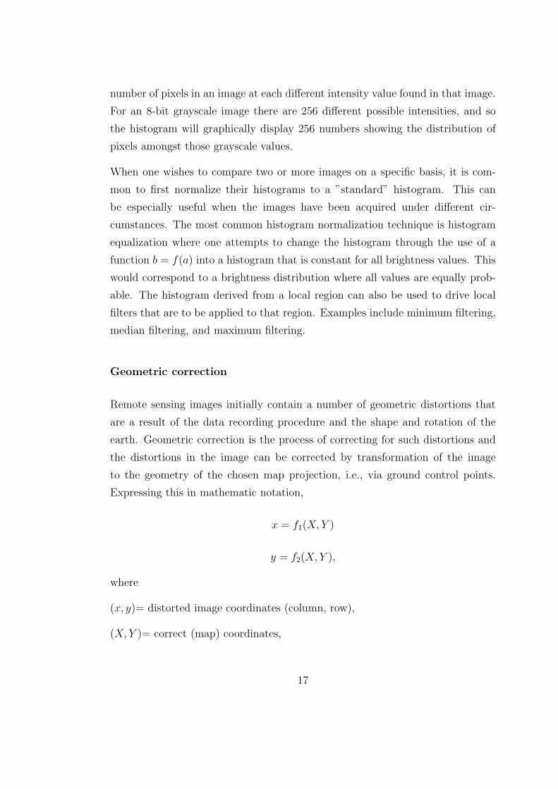
Geometric correction
Remote sensing images initially contain a number of geometric distortions that
are a result of the data recording procedure and the shape and rotation of the
earth. Geometric correction is the process of correcting for such distortions and
the distortions in the image can be corrected by transformation of the image
to the geometry of the chosen map projection, i.e., via ground control points.
Expressing this in mathematic notation,
x = f1(X, Y )
y = f2(X, Y ),
where
(x, y)= distorted image coordinates (column, row),
(X, Y )= correct (map) coordinates,
17

f1, f2 =transformation functions.
Note that some of the geometric distortions are usually corrected for by the data
distributor before delivery [47].
Radiometric correction
Digital images are a set of two dimensional rasters of digital numbers (DN).
Conversion of DNs to absolute radiance values - for any given channel - are
computed from
DN = gL + o, (2.3.1)
where
g = channel gain (slope),
L = spectral radiance measured over the spectral bandwith of the channel,
o = channel offset (intercept).
Major sources of error in the radiometric determination are (a) sun glint (MODIS
bands 20, 22, and 23), (b) water vapor absorption in the atmosphere (MODIS
bands 31, 32), [ atbd mod25 ]. Total spectral radiance [47] can be expressed by
Ltot =ρET
π+ Lp, (2.3.2)
where ρ = reflectance of target,
T = transmission of atmosphere,
Lp = path radiance, and
E = irradiance on the target.
= (E0cosθ0)/d2. Here d is the earth-sun distance, θ0 is the sun zenith angle,
and E0 is the solar irradiance at mean earth-sun distance.
18
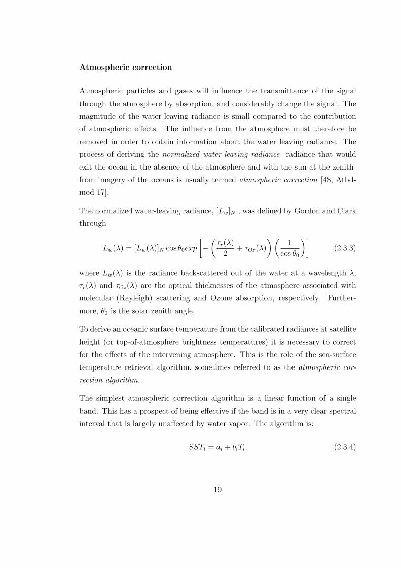
Atmospheric correction
Atmospheric particles and gases will influence the transmittance of the signal
through the atmosphere by absorption, and considerably change the signal. The
magnitude of the water-leaving radiance is small compared to the contribution
of atmospheric effects. The influence from the atmosphere must therefore be
removed in order to obtain information about the water leaving radiance. The
process of deriving the normalized water-leaving radiance -radiance that would
exit the ocean in the absence of the atmosphere and with the sun at the zenith-
from imagery of the oceans is usually termed atmospheric correction [48, Atbd-
mod 17].
The normalized water-leaving radiance, [Lw]N , was defined by Gordon and Clark
through
Lw(λ) = [Lw(λ)]N cos θ0exp
[−
(τr(λ)
2+ τOz(λ)
)(1
cos θ0
)](2.3.3)
where Lw(λ) is the radiance backscattered out of the water at a wavelength λ,
τr(λ) and τOz(λ) are the optical thicknesses of the atmosphere associated with
molecular (Rayleigh) scattering and Ozone absorption, respectively. Further-
more, θ0 is the solar zenith angle.
To derive an oceanic surface temperature from the calibrated radiances at satellite
height (or top-of-atmosphere brightness temperatures) it is necessary to correct
for the effects of the intervening atmosphere. This is the role of the sea-surface
temperature retrieval algorithm, sometimes referred to as the atmospheric cor-
rection algorithm.
The simplest atmospheric correction algorithm is a linear function of a single
band. This has a prospect of being effective if the band is in a very clear spectral
interval that is largely unaffected by water vapor. The algorithm is:
SSTi = ai + biTi, (2.3.4)
19
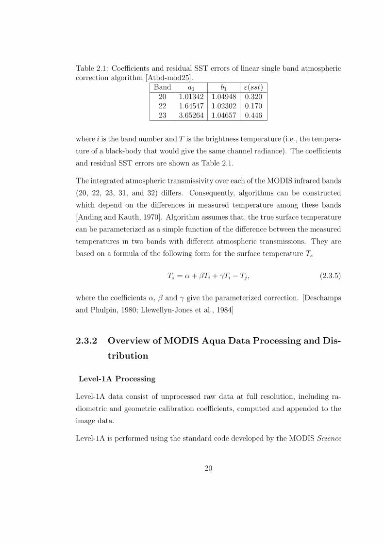
Table 2.1: Coefficients and residual SST errors of linear single band atmosphericcorrection algorithm [Atbd-mod25].
Band a1 b1 ε(sst)20 1.01342 1.04948 0.32022 1.64547 1.02302 0.17023 3.65264 1.04657 0.446
where i is the band number and T is the brightness temperature (i.e., the tempera-
ture of a black-body that would give the same channel radiance). The coefficients
and residual SST errors are shown as Table 2.1.
The integrated atmospheric transmissivity over each of the MODIS infrared bands
(20, 22, 23, 31, and 32) differs. Consequently, algorithms can be constructed
which depend on the differences in measured temperature among these bands
[Anding and Kauth, 1970]. Algorithm assumes that, the true surface temperature
can be parameterized as a simple function of the difference between the measured
temperatures in two bands with different atmospheric transmissions. They are
based on a formula of the following form for the surface temperature Ts
Ts = α + βTi + γTi − Tj, (2.3.5)
where the coefficients α, β and γ give the parameterized correction. [Deschamps
and Phulpin, 1980; Llewellyn-Jones et al., 1984]
2.3.2 Overview of MODIS Aqua Data Processing and Dis-
tribution
Level-1A Processing
Level-1A data consist of unprocessed raw data at full resolution, including ra-
diometric and geometric calibration coefficients, computed and appended to the
image data.
Level-1A is performed using the standard code developed by the MODIS Science
20

Data Support Team (SDST), known as MOD-PR01 (modis-l1agen in SeaDAS)
The output of MOD-PR01 is a 5-minute Level-1A granule in HDF format.These
standard Level-1A files are then reduced in the process called MY D − L1ASS,
where excess bands and data that are not utilized by Oceans are removed. The
resulting Level-1A files are smaller in size and easier to work with. The Level-1A
file format uses 16-bit integers to store the 12-bit data, so 4 bits of unused space
are available. Using correlation between the high resolution land bands and the
closest corresponding ocean bands, the counts stored in bands 10, 12, 13, and 16
were extended above their original 12-bit saturation limit up to the 16-bit limit
of the Level-1A format.
Geolocation
The next step in the processing involves generation of the geolocation.This is per-
formed using standard SDST code known as MOD-PR03 (geolocate in SeaDAS).
For the NRT stream, the predicted attitude and ephemeris files are used to pro-
duce Quick-Look GEO files.Several days later, in the Refined processing stream,
the definitive attitude and ephemeris files are used to create the final GEO version.
GEO files are not maintained in the long-term archive, since they can be regen-
erated as needed using the much smaller attitude and ephemeris files.Therefore,
only a short-term rolling archive is made available for distribution.
21

Level-1B
After the geolocation step, the Level-1A file and the GEO file for each 5-minute
granule are fed into MYD-PR02 (aqua - l1bgen in SeaDAS) to produce the cor-
responding Level-1B file.The standard MYD-PR02 code is developed and main-
tained by the MODIS Calibration Support Team (MCST). The standard Level-1B
format for 1-km data includes a pair of SDS fields for 250-meter and 500-meter
that have been aggregated to 1-km.Since the Ocean Level-1A does not include
the high-resolution bands, these aggregated fields would normally be unfilled.The
OBPG uses this free space to store the extended ocean band information from
bands 10, 12, 13lo, and 16, as these high reflectance values will not fit into the
standard scaled integer fields provided for the Level-1B reflectances.
Level-2
A Level-2 data product is a processed product where a sensitivity loss correction,
atmospheric correction, and chlorophyll derivation algorithm have bee applied to
a level 1 product to calculate surface reflectances, land/cloud flags, subsurface
reflectances, atmospheric signals, and chlorophyll concentration.
Level-2 processing is performed using the Multi-Sensor Level-1 to Level-2 (MSL12)
code and generates Level-2 geophysical products by applying atmospheric correc-
tions and bio-optical algorithms to the sensor data. The input data levels required
for msll2 processing for MODIS is the Level-1B file and the GEO file. The Level-2
processing also makes use of meteorological and ozone information from ancillary
sources. Figure 2.6 gives an overview of the MODIS data flow within the OBPG.
22
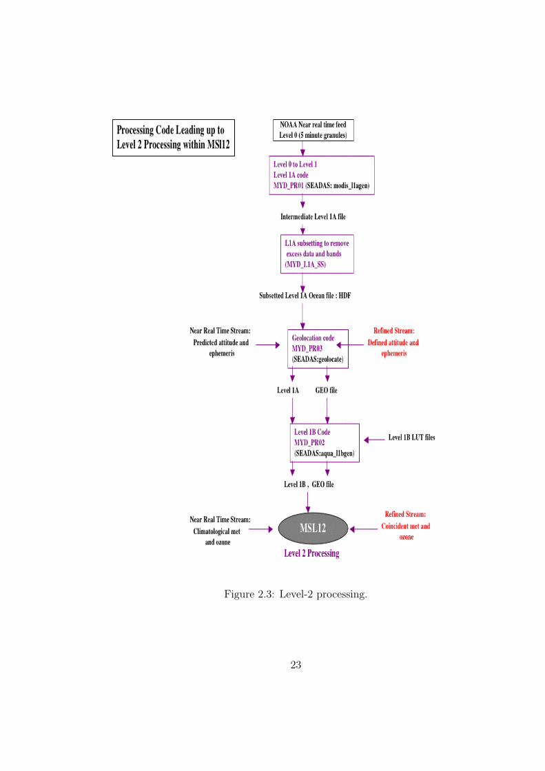
Figure 2.3: Level-2 processing.
23
2.3.3 Implementation of SST Processing
Short-wave SST Algorithm
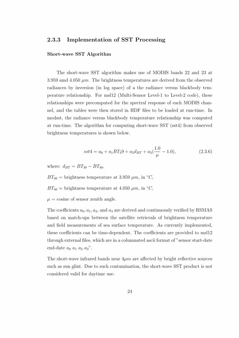
The short-wave SST algorithm makes use of MODIS bands 22 and 23 at
3.959 amd 4.050 µm. The brightness temperatures are derived from the observed
radiances by inversion (in log space) of a the radiance versus blackbody tem-
perature relationship. For msl12 (Multi-Sensor Level-1 to Level-2 code), these
relationships were precomputed for the spectral response of each MODIS chan-
nel, and the tables were then stored in HDF files to be loaded at run-time. In
modsst, the radiance versus blackbody temperature relationship was computed
at run-time. The algorithm for computing short-wave SST (sst4) from observed
brightness temperatures is shown below.
sst4 = a0 + a1BT39 + a2dBT + a3(1.0
µ− 1.0), (2.3.6)
where: dBT = BT39 −BT40,
BT39 = brightness temperature at 3.959 µm, in ◦C,
BT40 = brightness temperature at 4.050 µm, in ◦C,
µ = cosine of sensor zenith angle.
The coefficients a0, a1, a2, and a3 are derived and continuously verified by RSMAS
based on match-ups between the satellite retrievals of brightness temperature
and field measurements of sea surface temperature. As currently implemented,
these coefficients can be time-dependent. The coefficients are provided to msl12
through external files, which are in a columnated ascii format of ”sensor start-date
end-date a0 a1 a2 a3”.
The short-wave infrared bands near 4µm are affected by bright reflective sources
such as sun glint. Due to such contamination, the short-wave SST product is not
considered valid for daytime use.
24
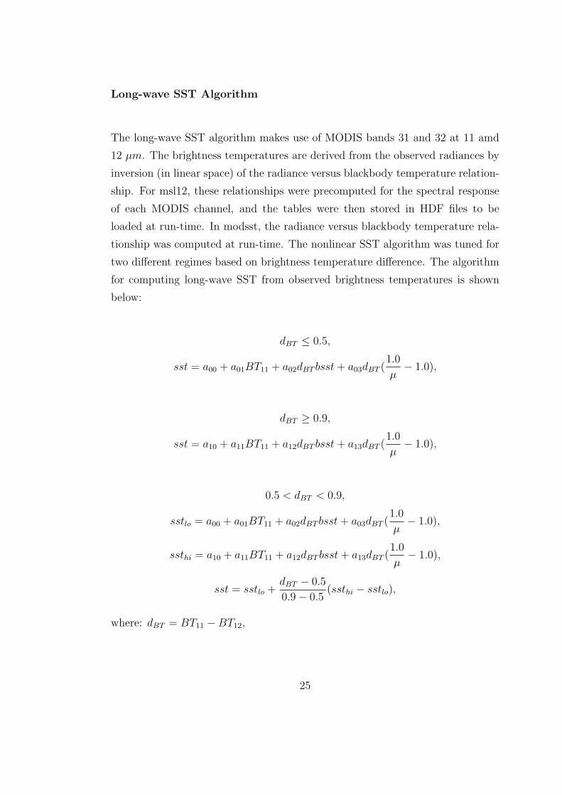
Long-wave SST Algorithm
The long-wave SST algorithm makes use of MODIS bands 31 and 32 at 11 amd
12 µm. The brightness temperatures are derived from the observed radiances by
inversion (in linear space) of the radiance versus blackbody temperature relation-
ship. For msl12, these relationships were precomputed for the spectral response
of each MODIS channel, and the tables were then stored in HDF files to be
loaded at run-time. In modsst, the radiance versus blackbody temperature rela-
tionship was computed at run-time. The nonlinear SST algorithm was tuned for
two different regimes based on brightness temperature difference. The algorithm
for computing long-wave SST from observed brightness temperatures is shown
below:
dBT ≤ 0.5,
sst = a00 + a01BT11 + a02dBT bsst + a03dBT (1.0
µ− 1.0),
dBT ≥ 0.9,
sst = a10 + a11BT11 + a12dBT bsst + a13dBT (1.0
µ− 1.0),
0.5 < dBT < 0.9,
sstlo = a00 + a01BT11 + a02dBT bsst + a03dBT (1.0
µ− 1.0),
ssthi = a10 + a11BT11 + a12dBT bsst + a13dBT (1.0
µ− 1.0),
sst = sstlo +dBT − 0.5
0.9− 0.5(ssthi − sstlo),
where: dBT = BT11 −BT12,
25

BT11 = brightness temperature at 11 µm in ◦C,
BT12 = brightness temperature at 12 µm, in ◦C,
bsst = baseline SST, which is either sst4 (if valid) or sstref (from oisst),
µ = cosine of sensor zenith angle.
At night, where sst4 retrieval is reliable, the algorithm uses sst4 for the bsst
value. For daytime SST, the algorithm uses a reference SST source (sstref) for
bsst, where sstref is operationally derived from the weekly Reynolds oisst product,
bilinearly interpolated to the pixel location. The coefficients a00, a01 , a02,a03 and
a10, a11, a12, and a13 are derived and continuously verified by RSMAS based
on match-ups between the satellite retrievals of brightness temperature and field
measurements of sea surface temperature.
MODIS homepage:
http://oceancolor.gsfc.nasa.gov/DOCS/modis sst/sst modisa.dat
2.3.4 MODIS ocean data processing codes
The main aim of the MODIS ocean processing code is to calculate level 2,
3, and 4 ocean products from level 1B satellite radiance data. This process is
performed in several stages, where the ocean color and sea-surface temperature
(SST) level 2 products are first calculated, followed by space and time-binning to
retrieve level 3 products, and statistical mapping to yield level 4 products.
The ocean color processing routine (MODCOL) includes atmospheric correction
algorithms to convert level 1B radiances to water-leaving radiances, as well as al-
gorithms to derive level 2 ocean color products such as chlorophyll concentration.
The code is divided into six main components:
MODCOL : performs atmospheric correction and applies the ocean color algo-
rithms to level 1B data,
26
MODSST : calculates the sea-surface temperature (SST) from level 1B data,
MSBIN : space bins the level 2 data,
MTBIN : time bins the level 2 data,
MFILL : calculates a 24-day reference,
MCLOUD : declouds the data,
and two auxiliary components:
MMAP : maps data onto geographic projections,
MSPC : changes the spatial resolution of the binned data.
We only pay attention to MODCOL and MODSST applied to our level 2 data to
improve accuracy. Level 1B data, geolocation data, ancillary data, cloud mask
data, aerosol data, water vapor data (SST calculations only) and 24-day SST
reference data (SST calculations only), are input into MODCOL and MODSST.
MODCOL
This program processes level 1B data, creating level 2 ocean color data products.
The program first applies atmospheric correction to the level 1B data, and then
estimates a suite of ocean color products using a number of ocean color algorithms.
Level 1B satellite data, geolocation data, cloud mask data and aerosol data are
obtained from the satellite data itself. Ancillary data (algorithm coefficients,
meteorology, ozone, etc.) are obtained from external files.
MODSST
This program calculates level 2 sea-surface temperature (SST) products from
level 1B satellite data. It calls the main subroutine modsstmain which calls the
remaining subroutines.
The input files required for processing of SST data are:
27

level 1B satellite data,
geolocation data,
cloud mask data,
aerosol data,
water vapor,
24-day SST reference OR Reynolds SST data (currently used),
ancillary data (algorithm coefficients, meteorology, ozone, etc.).
The first five files are obtained from the satellite data itself.
Each of these programs outputs -in hdf file- contain the indicated ocean color
products as well as metadata. Metadata contain auxiliary information such as
the creation date, datatime, principal investigator, sensor characteristics, algo-
rithms used, etc. [http : //modis.gsfc.nasa.gov/data/algorithms.html].
Full documentation, updated code source, sensor files, and output product de-
scriptions can be found at http://oceancolor.gsfc.nasa.gov/DOCS and MODIS
home page
In this study, SST-night (4µm) and sst-day (12µm) MODIS Aqua data were
used. Before using these hdf (hierachical data format) type data we use several
techniques to gain meaningful form of SST, quality level, l2-flags, latitude and
longitude. (See Appendix A for converthdf.m.)
28

chapter 3
MATHEMATICAL
BACKGROUND
3.1 Introduction to Vectors and Matrices
A real N−dimensional vector X is an ordered set of N real numbers and is
usually written in the coordinate form
X = (x1, x2, . . . , xN).
Here the numbers x1, x2, . . . , and xN are called the components of X. The set
consisting of all N− dimensional vectors is called N −dimensional space. When
a vector is used to denote a point or position in space, it is called position vector.
When it is used to denote a movement between two points in space, it is called a
displacement vector.
Let another vector be Y = (y1, y2, . . . , yN). The two vectors X and Y are said to
be equal if and only if each corresponding coordinate is the same.
The sum of the vectors X and Y is computed component by component.
The negative of the vector X is obtained by replacing each coordinate with its
negative.
The difference Y −X is formed by taking the difference in each coordinate.
29

Vectors in N -dimensional space obey the algebraic property
Y −X = Y + (−X).
If c is a real number (scalar), we define scalar multiplication cX as follows:
cX = (cx1, cx2, . . . , cxN).
If c and d are scalars, then the weighted sum cX+dY is called a linear combination
of X and Y and we write
cX + dY = (cx1 + dy1, cx2 + dy2, . . . , cxN + dyN).
The dot product of the two vectors X and Y is a scalar quantity (real number)
defined by the equation
X · Y = x1y1 + x2y2 + . . . + xNyN .
The norm (or length) of the vector X is defined by
‖X‖ =√
x21 + x2
2 + . . . + x2N .
An important relationship exists between the dot product and norm of a vector.
Using last two equations we have
‖X‖2 = x21 + x2
2 + . . . + x2N = X ·X.
The formula for the distance between two points in N -space is
‖Y −X‖ =√
(y1 − x1)2 + (y2 − x2)2 + . . . + (yN − xN)2.
30

3.1.1 Matrices and Two-dimensional Arrays
A matrix is a rectangular array of numbers that is arranged systematically
in rows and columns. A matrix having M rows and N columns is called an
M ×N (read ”M by N”) matrix. The capital letter A denotes a matrix, and the
lowercase subscripted letter aij denotes one of the numbers forming the matrix.
We write
A = [aij]MxN .
We refer to aij as the entry in location (i, j).
The rows of the M ×N matrix A are N−dimensional vectors:
Vi = (ai1, ai2, . . . , aiN) for i = 1, 2, . . . , M.
In expanded form we write
a11 a12 . . . a1j . . . a1N
a21 a22 . . . a2j . . . a2N
......
......
ai1 ai2 . . . aij . . . aiN
......
......
aM1 aM2 . . . aMj . . . aMN
= A
Let A = [aij]M×N and B = [bij]M×N be two matrices of the same dimension.
The two matrices A and B are said lo be equal if and only if each corresponding
element is the same; that is,
A = B if and only if aij = bij for 1 ≤ i ≤ M, 1 ≤ j ≤ N.
The sum of the two M ×N matrices A and B is computed element by element,
31

using the definition
A + B = [aij + bij]MxN for 1 ≤ i ≤ M, 1 ≤ j ≤ N.
The negative of the matrix A is obtained by replacing each element with its
negative:
−A = [−aij]MxN for 1 ≤ i ≤ M, 1 ≤ j ≤ N.
The difference AB is formed by taking the difference of corresponding coordinates:
A−B = [aij − bij]MxN for 1 ≤ i ≤ M, 1 ≤ j ≤ N.
If c is a real number (scalar), we define scalar multiplication cA as follows:
cA = [caij]MxN for 1 ≤ i ≤ M, 1 ≤ j ≤ N.
If p and q are scalars, the weighted sum pA + qB is called a linear combination
of the matrices A and B, and we write
pA + qB = [paij + qbij]MxN for 1 ≤ i ≤ M, 1 ≤ j ≤ N.
3.1.2 Properties of Vectors and Matrices
A linear combination of the variables x1, x2, . . . , xN is a sum
a1x1 + a2x2 + . . . + aNxN ,
where ak is the coefficient of xk for k = 1, 2, . . . , N .
A linear equation in x1, x2, . . . , xN is obtained by requiring the linear combination
32
in the previous equation to take on a prescribed value b; that is,
a1x1 + a2x2 + . . . + aNxN = b.
Systems of linear equations arise frequently, and if M equations in N unknowns
are given, we write
a11x1 + a12x2 + . . . + a1NxN = b1
a21x1 + a22x2 + . . . + a2NxN = b2
......
......
ak1x1 + ak2x2 + . . . + akNxN = bk
......
......
aM1x1 + aM2x2 + . . . + aMNxN = bM
A solution to this is a set of numerical values x1, x2, . . . , xN that satisfies all the
equations in simultaneously. Hence a solution can be viewed as an N−dimensional
vector;
X = (x1, x2, . . . , xN) .
We now discuss how to use matrices to represent a linear system of equations.
The linear equations above can be written as a matrix product. The coefficients
akj are stored in a matrix A (called the coefficient matrix ) of dimension M ×N ,
and the unknowns xj are stored in a matrix X of dimension N×1, The constants
bk are stored in a matrix B of dimension M × 1. It is conventional to use column
33

matrices for both X and B and we write
AX =
a11 a12 . . . a1j . . . a1N
a21 a22 . . . a2j . . . a2N
......
......
ak1 ak2 . . . akj . . . akN
......
......
aM1 aM2 . . . aMj . . . aMN
x1
x2
...
xj
...
xN
=
b1
b2
...
bj
...
bM
= B.
The matrix multiplication AX = B is reminiscent of the dot product for ordinary
vectors, because each element bk in B is the result obtained by taking the dot
product of row k in matrix A with the column matrix X.
3.1.3 Solutions to Systems of Linear Equations
The following is an example of a system of three linear equations with three
unknowns (x1, x2, x3):
3x1 +2x2 −x3 =10
−x1 +3x2 +2x3 =5
x1 −x2 −x3 =− 1
This system of equations can be rewritten in matrix form as
Ax =
3 2 −1
−1 3 2
1 −1 −1
x1
x2
x3
=
10
5
−1
= B.
The system of equations is nonsingular if the matrix A containing the coefficients
of the equations is nonsingular. The rank of A must be equal to the number of
rows of A and the determinant |A| must be nonzero for the system of equations
to be nonsingular.
34
Solution by Matrix Inverse
Premultiply the system of equations Ax = b by A−1
A−1Ax = A−1b.
Because A−1A is equal to the identity matrix I [19]
Ix = A−1b or x = A−1b.
We can use this method if A is a square matrix. If A is not square, a M × N
matrix pseudoinverse operator A+ may be used to determine a solution.
Pseudoinverse Operators
The first type of pseudoinverse operator to be introduced is the generalized
inverse A−, which satisfies the following relations [14]:
AA− = [AA−]T ,
A−A = [A−A]T ,
AA−A = A,
A−AA− = A−.
The generalized inverse is unique. It may be expressed explicitly under certain
circumstances. If M > N , the system is said to be overdetermined ; that is, there
are more observations than points to be estimated. In this case, if A is of rank
N , the generalized inverse may be expressed as
A− = [AT A]−1AT .
At the other extreme, if M < N the system is said to be underdetermined. In
this case, if A is of rank M , the generalized inverse is equal to
A− = AT [AT A]−1.
35
Another type of pseudoinverse operator is the least-squares inverse A§, which
satisfies the defining relations
AA§A = A,
AA§ = [AA§]T .
Finally, a conditional inverse A] is defined by the relation
AA]A = A.
Examination of the defining relations for the three types of pseudoinverse opera-
tors reveals that the generalized inverse is also a least-squares inverse, which in
turn is also a conditional inverse. Least-squares and conditional inverses exist
for a given linear operator A; however, they may not be unique. Furthermore, it
is usually not possible to explicitly express these operators in closed form. The
following is a list of useful relationships for the generalized inverse operator of a
M ×Nmatrix A [8].
3.1.4 Singular Value Matrix Decomposition (SVD)
Any arbitrary M ×N matrix A of rank R can be decomposed into the sum
of a weighted set of unit rank M ×N matrices by a singular-value decomposition
(SVD).
According to the SVD matrix decomposition, there exist an M ×M unitary
matrix U and an N ×N unitary matrix V for which
UT AV = Λ1/2
36
where
Λ1/2 =
λ1/2(1) . . . 0...
. . ....
λ1/2(1)
0 . . . 0
is an M×N matrix with a general diagonal entry λ1/2(j) called a singular value of
A. Since U and V are unitary matrices, UUT = IM and V V T = IN . Consequently,
A = UΛ1/2V T .
3.2 Interpolation and Curve Fitting
The very processes of interpolation and curve fitting are basically attempts to
get ”something for nothing”. In general, one has a function defined at a discrete
set of points and desires information about the function at some other point.
Well that information simply does not exist. One must make some assumptions
about the behavior of the function. This is where some of the ”art of computing”
enters the picture. One needs some knowledge of what the discrete entries of
the table represent. In picking an interpolation scheme to generate the missing
information, one makes some assumptions concerning the functional nature of
the tabular entries. That assumption is that they behave as polynomials. All
interpolation theory is based on polynomial approximation [19, 21].
Precisely, given n + 1 pairs (tk, x(tk)), the problem consists of finding a function
p = p(t) such that p(tk) = x(tk) for i = 0, . . . , m, x(tk) being some given values,
and say that p interpolates x(tk) at the nodes tk. We speak about polynomial
interpolation if p is an algebraic polynomial, trigonometric approximation if p
is a trigonometric polynomial or piecewise polynomial interpolation (or spline
interpolation) if p is only locally a polynomial [14].
The problem of finding x(t, α) -to minimize the error
37

e(tk) = x(tk)− x(tk, α) , (k ∈ Zn+1), (3.2.1)
where α is the vector of unknown parameters- is often called curve fitting. Curve
fitting is used when the data are uncertain because of the corrupting effects of
measurement errors, random noise, or interference. Interpolation is appropriate
when the data are accurately or exactly known.
Interpolation is quite important in processing. For example, bandlimited signals
may need to be interpolated in order to change sampling rates. Interpolation is
vital in numerical integration methods, as will be seen later. In this application
the integrand is typically known or can be readily found at some finite set of
points with significant accuracy. Interpolation at these points leads to a function
(usually a polynomial) that can be easily integrated, and so provides a useful
approximation to the given integral.
3.2.1 Lagrange Interpolation
Assume that we wish to interpolate the data set {(tk, xk)|k ∈ Zn+1}. Suppose that
we possess polynomials (called Lagrange polynomials) Lj(t) with the property
Lj(tk); =
(0 , j 6= k
1 , j = k
)= δj−k. (3.2.2)
Then the interpolating polynomial for the data set is
pn(t) = x0L0(t) + x1L1(t) + . . . + xnLn(t) =n∑
j=0
xjLj(t). (3.2.3)
We observe that
pn(tk) =n∑
j=0
xjLj(tk) =n∑
j=0
xjδj−k = xk (3.2.4)
38

for k ∈ Zn+1 so pn(t) in (3.2.6) does indeed interpolate the data set. We may see
that for j ∈ Zn+1 the Lagrange polynomials are given by
Lj(t) =n∏
i=0
t− titj − ti
, i 6= j. (3.2.5)
Equation (3.2.6) is called the Lagrange form of the interpolating polynomial [37].
3.2.2 Newton Interpolation
Define
x[t0.t1] =x(t1)− x(t0)
t1 − t0=
x1 − x0
t1 − t0. (3.2.6)
This is called the first divided difference of x(t) relative to t1 and t0. We see that
x[t0, t1] = x[t1, t0]. We may linearly interpolate x(t) for t ∈ [t0, t1] according to
x(t) ≈ x(t0) +t− t0t1 − t0
[x(t1)− x(t0)] = x(t0) + (t− t0)x[t0, t1]. (3.2.7)
It is convenient to define p0(t) = x(t0) and p1(t) = x(t0) + t − t0x[t0, t1] (it is
consistent with previous section). In fact, p1(t) agrees with the solution to
[1 t0
1 t1
] [p1,0
p1,1
]=
[x0
x1
](3.2.8)
as we expect.
Unless x(t) is truly linear the secant slope x[t0, t1] will depend on the abscissas
t0 and t1 If xt is a second degree polynomial then x[t1, t] will itself be a linear
function of t for a given t1. Consequently, the ratio
x[t0, t1, t2] =x[t1, t2]− x[t0, t1]
t2 − t0(3.2.9)
will be independent of t0, t1, and t2. (This ratio is the second divided difference
of x(t) with respect to t0, t1, and t2.)
39

x(t) ≈ x(t0) + (t− t0)x[t0, t1] + (t− t0)(t− t1)x[t0, t1, t2] = p2(t) (3.2.10)
is the second-degree interpolation formula, while (3.2.10) is the first-degree inter-
polation formula.
Continuing in this fashion, we obtain
x(t) = x[t0] + (t− t0)x[t0, t1] + (t− t0)(t− t1)x[t0, t1, t2] + . . .
+(t− t0)(t− t1) . . . (t− tn−1)x[t0, t1, . . . , tn] + e(t), (3.2.11)
where
e(t) = (t− t0)(t− t1) . . . (t− tn)x[t0, t1, . . . , tn, t], (3.2.12)
and we define
pn(t) = x[t0] + (t− t0)x[t0, t1] + (t− t0)(t− t1)x[t0, t1, t2] + . . .
+(t− t0) . . . (t− tn−1)x[t0, . . . , tn], (3.2.13)
which is the nth-degree interpolating formula, and is clearly a polynomial of degree
n. So e(t) is the error involved in interpolating x(t) using polynomial pn(t).
Equation (3.2.11) is the Newton interpolating formula with divided differences.If
x(t) is a polynomial of degree n (or less), then e(t) = 0 (for all t).
3.2.3 Spline Interpolation
Splines are interpolative polynomials that involve information concerning the
derivative of the function at certain points. Unlike Hermite interpolation that
explicitly invokes knowledge of the derivative, splines utilize that information
implicitly so that specific knowledge of the derivative in not required. Unlike
general interpolation formulae of the Lagrangian type, which maybe used in a
40

small section of a table, splines are constructed to fit an entire run of tabular
entries of the independent variable. While one can construct splines of any order,
the most common ones are cubic splines as they generate tri-diagonal equations
for the coefficients of the polynomials [8, 21]. Chapter 5 includes details of spline
interpolation.
Speed, Memory, and Smoothness Considerations
When choosing an interpolation method, we should keep in mind that some re-
quire more memory or longer computation time than others.
Nearest neighbor interpolation is the fastest method. However, it provides the
worst results in terms of smoothness. This method sets the value of an interpo-
lated point to the value of the nearest data point. Therefore, this method does
not generate any new data points.
Linear interpolation uses more memory than the nearest neighbor method, and
requires slightly more execution time. Unlike nearest neighbor interpolation its
results are continuous, but the slope changes at the vertex points.
Cubic spline interpolation has the longest relative execution time, although it
requires less memory than cubic interpolation. It produces the smoothest results
of all the interpolation methods. You may obtain unexpected results, however,
if your input data is non-uniform and some points are much closer together than
others.
Cubic interpolation requires more memory and execution time than either the
nearest neighbor or linear methods. However, both the interpolated data and its
derivative are continuous [10, 11].
3.3 Mathematical Morphology
The field of mathematical morphology contributes a wide range of operators
to image processing, all based around a few simple mathematical concepts from
41

set theory. The operators are particularly useful for the analysis of binary images
and common usages include edge detection, noise removal, image enhancement
and image segmentation.
The two most basic operations in mathematical morphology are erosion and di-
lation. Both of these operators take two pieces of data as input: an image to be
eroded or dilated, and a structuring element (also known as a kernel). The two
pieces of input data are each treated as representing sets of coordinates in a way
that is slightly different for binary and grayscale images [45].
Erosion and dilation work (at least conceptually) by translating the structuring
element to various points in the input image, and examining the intersection
between the translated kernel coordinates and the input image coordinates. Vir-
tually all other mathematical morphology operators can be defined in terms of
combinations of erosion and dilation along with set operators such as intersection
and union. Some of the more important are opening, closing and skeletonization.
3.3.1 Dilation
Dilation is one of the two basic operators in the area of mathematical mor-
phology, the other being erosion. It is typically applied to binary images, but
there are versions that work on grayscale images. The basic effect of the operator
on a binary image is to gradually enlarge the boundaries of regions of foreground
pixels (i.e., white pixels, typically). Thus areas of foreground pixels grow in size
while holes within those regions become smaller.
The dilation operator takes two pieces of data as inputs. The first (A) is the image
which is to be dilated. The second (B) is a (usually small) set of coordinate points
known as a structuring element (also known as a kernel). It is this structuring
element that determines the precise effect of the dilation on the input image.
The techniques of morphological filtering can be extended to gray-level images.
To simplify matters we will restrict our presentation to structuring elements that
42

comprise a finite number of pixels and are convex and bounded. Now, however,
the structuring element has gray values associated with every coordinate position
as does the image A [11, 45].
D(A,B) := max[j,k]∈B
a[m− j, n− k] + b[j, k]. (3.3.14)
For a given output coordinate [m,n], the structuring element is summed with a
shifted version of the image and the maximum encountered over all shifts within
the J ×K domain of B is used as the result.
3.3.2 Erosion
The basic effect of the operator on a binary image is to erode away the
boundaries of regions of foreground pixels (i.e., white pixels, typically). Thus
areas of foreground pixels shrink in size, and holes within those areas become
larger:
E(A,B) := min[j,k]∈B
a[m + j, n + k] + b[j, k]. (3.3.15)
For a given output coordinate [m,n], the structuring element is summed with a
shifted version of the image and the maximum encountered over all shifts within
the J x K domain of B is used as the result [45].
3.3.3 Opening and closing
Opening and closing are two important operators from mathematical mor-
phology. They are both derived from the fundamental operations of erosion and
dilation. The basic effect of an opening is somewhat like erosion in that it tends
to remove some of the foreground (bright) pixels from the edges of regions of
foreground pixels. However, it is less destructive than erosion in general. Closing
43

is similar in some ways to dilation in that it tends to enlarge the boundaries of
foreground (bright) regions in an image (and shrink background color holes in
such regions), but it is less destructive of the original boundary shape. Closing
is the dual of opening, i.e., closing the foreground pixels with a particular struc-
turing element, is equivalent to closing the background with the same element
[11].
44
chapter 4
INTRODUCTION TO IMAGE
PROCESSING
In this chapter we will briefly summarize digital image processing techniques
for edge detection, segmentation and reconstruction. Detailed methods used or
compared in this thesis can be found in Chapter 5.
4.1 Edge Detection
Edges are areas in an image where rapid changes occur in the intensity
function or in spatial derivatives of this intensity function which could be due to
discontinuities in scene reflectance, surface orientation, or depth [16]. Image pixels
representing such discontinuities carry more information than pixels representing
gradual change or no change in intensities.
The base of edge detection is differentiation. Note that the detected edge is the
derivative of the edge. This means it is the slope or rate of change of the gray
levels in the edge. The slope of the edge is always positive or zero, and it reaches
its maximum at the edge. For this reason, edge detection is often called image
differentiation.
45

The gradient of an image f at location (x, y), along the line normal to the edge
slope, is the vector
∇f =
[fx
fy
]=
[∂f∂x∂f∂y
]. (4.1.1)
The spatial gradient amplitude is given by:
G(x, y) =√
f 2x + f 2
y (4.1.2)
and the gradient direction with respect to the row axis is
Θ(x, y) = arctanfy
fx
. (4.1.3)
The first order derivative edge detection can be carried out either by using two
orthogonal directions in an image or by using a set of directional derivatives.
Thresholding and thinning : The most commonly used method of producing
edge segments or contours from (4.1.2) consists of two stages: thresholding and
thinning. In the thresholding stage, the gradient magnitude at every point is
compared to a predefined threshold value, T . All points satisfying the following
criterion are classified as candidate edge points:
|∇f(x, y)| ≥ T.
The set of candidate edge points tends to form strips, which have positive width.
Since the desire is usually for zero-width boundary segments or contours to de-
scribe the edges, a subsequent processing stage is needed to thin the strips to the
final edge contours. Edge contours derived from continuous-space images should
have zero width because any local maxima of |∇f(x, y)|, along a line segment
that crosses the edge, cannot be adjacent points.
46

The selection of the threshold value T is a tradeoff between the wish to fully
capture the actual edges in the image and the desire to reject noise. Increasing
T decreases sensitivity to noise at the cost of rejecting the weakest edges, forcing
the edge segments to become more broken and fragmented. By decreasing T,
one can obtain more connected and richer edge contours, but the greater noise
sensitivity is likely to produce more false edges.
Edge thinning can be accomplished in a number of ways, depending on the ap-
plication, but thinning by nonmaximum suppression is usually the best choice.
Generally speaking, we wish to suppress any point that is not, in a 1-D sense, a
local maximum in gradient magnitude. Since a 1−D local neighborhood search
typically produces a single maximum, those points that are local maxima will
form edge segments only one point wide. One approach classifies an edge-strip
point as an edge point if its gradient magnitude is a local maximum in at least
one direction. However, this thinning method sometimes has the side effect of
creating false edges near strong edge lines. It is also somewhat inefficient because
of the computation required to check along a number of different directions. A
better, more efficient thinning approach checks only a single direction, the gra-
dient direction, to test whether a given point is a local maximum in gradient
magnitude. The points that pass this scrutiny are classified as edge points. The
method is efficient because it is not necessary to search in multiple directions. It
also tends to produces edge segments having good localization accuracy. These
characteristics make the gradient direction, local extremum method quite popu-
lar. The following steps summarize its implementation.
1. Compute ∇f for all pixels.
2. Determine candidate edge pixels by thresholding all pixels gradient magnitudes
by T .
3. Thin by checking whether each candidate edge pixels gradient magnitude is
a local maximum along its gradient direction. If so, classify it as an edge pixel [51].
47
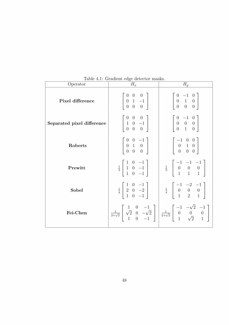
Table 4.1: Gradient edge detector masks.Operator Hx Hy
Pixel difference
0 0 00 1 −10 0 0
0 −1 00 1 00 0 0
Separated pixel difference
0 0 01 0 −10 0 0
0 −1 00 0 00 1 0
Roberts
0 0 −10 1 00 0 0
−1 0 00 1 00 0 0
Prewitt 13
1 0 −11 0 −11 0 −1
1
3
−1 −1 −10 0 01 1 1
Sobel 14
1 0 −12 0 −21 0 −1
1
4
−1 −2 −10 0 01 2 1
Fei-Chen 12+√
2
1 0 −1√2 0 −√2
1 0 −1
1
2+√
2
−1 −√2 −10 0 0
1√
2 1
48
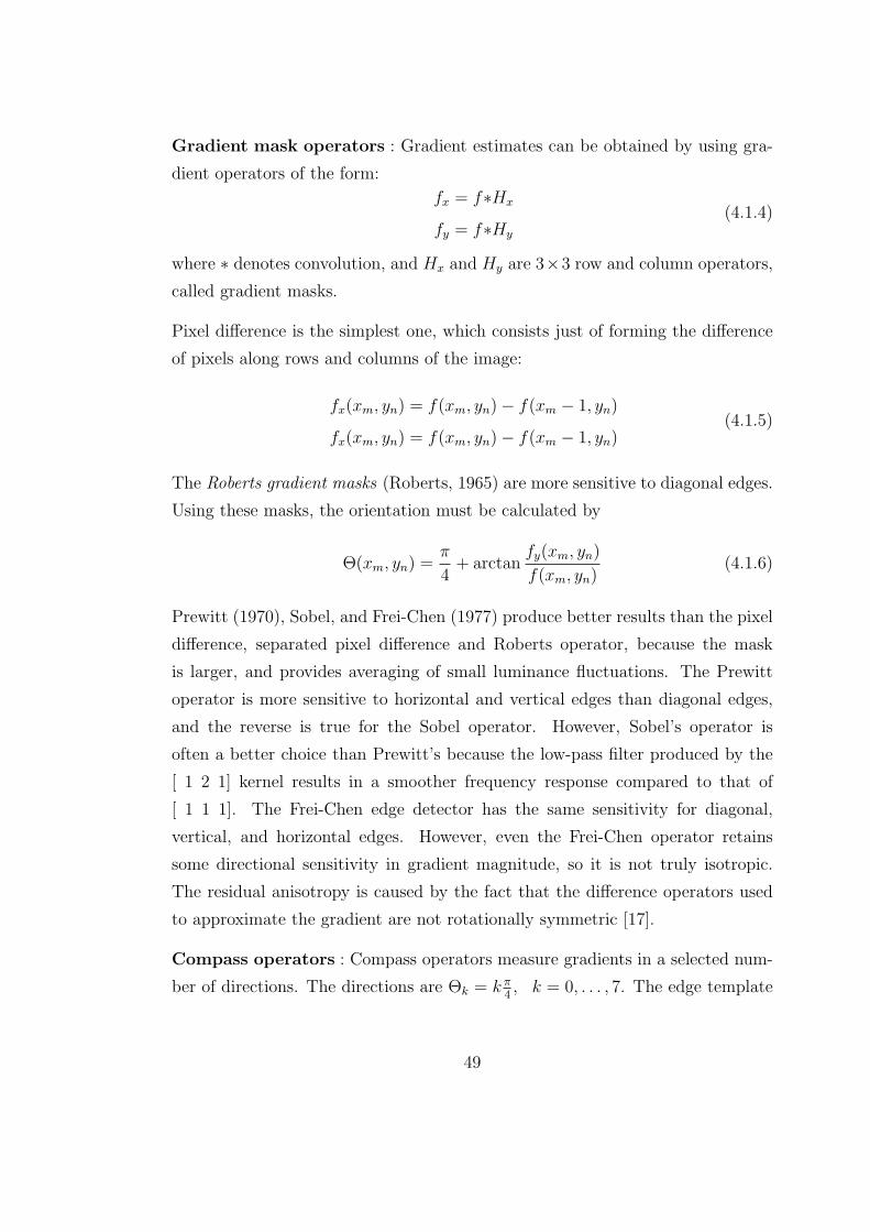
Gradient mask operators : Gradient estimates can be obtained by using gra-
dient operators of the form:
fx = f∗Hx
fy = f∗Hy
(4.1.4)
where ∗ denotes convolution, and Hx and Hy are 3×3 row and column operators,
called gradient masks.
Pixel difference is the simplest one, which consists just of forming the difference
of pixels along rows and columns of the image:
fx(xm, yn) = f(xm, yn)− f(xm − 1, yn)
fx(xm, yn) = f(xm, yn)− f(xm − 1, yn)(4.1.5)
The Roberts gradient masks (Roberts, 1965) are more sensitive to diagonal edges.
Using these masks, the orientation must be calculated by
Θ(xm, yn) =π
4+ arctan
fy(xm, yn)
f(xm, yn)(4.1.6)
Prewitt (1970), Sobel, and Frei-Chen (1977) produce better results than the pixel
difference, separated pixel difference and Roberts operator, because the mask
is larger, and provides averaging of small luminance fluctuations. The Prewitt
operator is more sensitive to horizontal and vertical edges than diagonal edges,
and the reverse is true for the Sobel operator. However, Sobel’s operator is
often a better choice than Prewitt’s because the low-pass filter produced by the
[ 1 2 1] kernel results in a smoother frequency response compared to that of
[ 1 1 1]. The Frei-Chen edge detector has the same sensitivity for diagonal,
vertical, and horizontal edges. However, even the Frei-Chen operator retains
some directional sensitivity in gradient magnitude, so it is not truly isotropic.
The residual anisotropy is caused by the fact that the difference operators used
to approximate the gradient are not rotationally symmetric [17].
Compass operators : Compass operators measure gradients in a selected num-
ber of directions. The directions are Θk = k π4, k = 0, . . . , 7. The edge template
49
gradient is defined as:
G(xm, yn) =7
maxk=0
|f(xm, yn)∗Hk(xm, yn)|. (4.1.7)
The Kirsch, Prewitt, and Sobel masks are compass gradient or directional edge
detectors. Given a pixel, there are eight directions to travel to a neighboring pixel
(above, below, left, right, upper left, upper right, lower left, and lower right). This
means that each of the eight masks detects an edge in one direction. Therefore,
there are eight possible directions for an edge. The directional edge detectors
can detect an edge in only one of the eight directions. To detect only left to
right edges, use only one of the eight masks. To detect all of the edges, perform
convolution over an image eight times using each of the eight masks [18].
Derivative of Gaussian :
The previous methods are relatively sensitive to the noise. A solution could be to
extend the window size of the gradient mask operators. Another approach is to
use the derivative of the convolution of the image by a Gaussian. The derivative
of a Gaussian (DroG) operator is
∇(g∗f) =∂(g∗f)
∂x+
∂(g∗f)
∂y= fx + fy (4.1.8)
with g = e−x2+y2
2σ2 Partial derivatives of the Gaussian function are
gx(x, y) =− x
σ2g,
gy(x, y) =− y
σ2g.
The filters are separable so we have [17]
gx(x, y) = gx(x)∗g(y),
gy(x, y) = gy(y)∗g(x).
50

Table 4.2: Masks for Edge Detection [18]Kirsch Prewitt Sobel
5 5 5−3 0 −3−3 −3 −3
1 1 11 −2 1−1 −1 −1
1 2 10 0 0−1 −2 −1
−3 5 5−3 0 5−3 −3 −3
1 1 11 −2 −11 −1 −1
2 1 01 0 −10 −2 −2
−3 −3 5−3 0 5−3 −3 5
1 1 −11 −2 −11 1 −1
1 0 −12 0 −21 0 −1
−3 −3 −3−3 0 5−3 5 5
1 −1 −11 −2 −11 1 1
0 −1 −21 0 −12 1 0
−3 −3 −3−3 0 −35 5 5
−1 −1 −11 −2 11 1 1
−1 −2 −10 0 01 2 1
−3 −3 −35 0 −35 5 −3
−1 −1 1−1 −2 11 1 1
−2 −1 0−1 0 10 1 2
5 −3 −35 0 −35 −3 −3
−1 1 1−1 −2 1−1 1 1
−1 0 1−2 0 21 0 1
5 5 −35 0 −3−3 −3 −3
1 1 1−1 −2 1−1 −1 1
0 1 2−1 0 1−2 −1 0
51

Thenfx = gx(x)∗g(y)∗f,
fy = gy(y)∗g(x)∗f.
52
4.2 Segmentation
The word segmentation has two meanings: the procedure leading to the
segmented image, and the result of such a procedure. Image segmentation is
the division of an image into spatially continuous, disjointed and homogeneous
regions, such that the pixels in each partitioned region possess an identical set
of properties or attributes. A complete segmentation of an image R involves
identification of a finite set of regions (R1, R2, R3, . . . , RN) such that
1) R = R1 ∪R2 ∪R3 ∪ . . . ∪RN ,
2) Ri ∩Rj = ∅, ∀i 6= j,
3) P (Ri) = True, ∀i,
4) P (Ri ∪Rj) = False, i 6= j.
Because of the variety and complexity of images, robust and efficient segmen-
tation algorithm on digital images is still a very challenging research topic and
fully automatic segmentation procedures are far from satisfying in many realistic
situations. Nevertheless general approaches to segmentation can be grouped into
three classes: pixel-based methods, regional methods, and edge based methods.
Pixel-based methods are the easiest to understand and to implement, but are also
the least powerful and, since they operate on one element at time, are particu-
larly susceptible to noise. Continuity-based and edge-based methods approach
the segmentation problem from opposing sides: edge-based methods search for
differences while continuity-based methods search for similarities.
4.2.1 Pixel Based Segmentation
The most straightforward and common of the pixel-based methods is thresh-
olding in which all pixels having intensity values above, or below, some level are
classified as part of the segment [4]. The selection of an appropriate threshold
value is usually based on a priori known properties of the object and background.
53
Even though image thresholding may, in many cases, seem trivial that is not
usually the case. The contrast between the objects may be poor and the illu-
mination conditions may vary and cause artefacts (such as shadows) that make
the determination of appropriate threshold difficult. In addition, many applica-
tions require that the appropriate thresholds can be determined automatically [3,
11]. Image thresholding is naturally more suitable when the object intensities are
smooth and almost constant inside the segments; otherwise, it fails or at least
produces rough and imprecise borders with many erratically classified areas. [5]
In bi-level thresholding, the object and background form two different groups
with distinct gray levels. All gray values greater than threshold T are assigned
the object label and all other gray values are assigned the background label, thus
separating the object pixels from the background pixels. In multi-level thresh-
olding, the image is partitioned into different segments using multiple threshold
values. In the first stage of the process, the image is thresholded to separate
brighter regions from darker regions by locating a minimum between luminance
modes of the histogram. Then histograms are formed of each of the segmented
parts. If these histograms are not unimodal, the parts are thresholded again. The
process continues until the histogram of a part becomes unimodal [6, 8].
4.2.2 Edge Based Segmentation
Historically, edge-based methods were the first set of tools developed for seg-
mentation. To move from edges to segments, it is necessary to group edges into
chains that correspond to the sides of structural units, i.e., the structural bound-
aries. Approaches vary in how much prior information they use, that is, how
much is used of what is known about the possible shape. False edges and missed
edges are two of the more obvious, and more common, problems associated with
this approach. The first step in edge-based methods is to identify edges which
then become candidates for boundaries.
When the boundaries are determined properly, they are formed by closed curves
54

and the interior of such a curve is then the sought area of a segment. In a sense,
this approach also utilizes the idea of homogeneity of segmented regions; however,
the requirements are much weaker: the edge is detected at locations where there
is an abrupt change in the image properties, thus indicating a probable region
border.
The detected region borders should be continuous and closed, reliable, and should
describe the perimeters of regions with a good accuracy of localization. Unfor-
tunately, the raw edge representation of an image as obtained by most edge de-
tection techniques are usually far from this ideal. The obtained edges are usually
disconnected, sometimes multiple or excessively thick, and many of the detected
edges do not correspond to segment borders, but rather to spurious rims due to
noise [5, 11].
If an image is noisy or if its region attributes differ by only a small amount between
regions, a detected boundary may often be broken. Edge linking techniques can
be employed to bridge short gaps in such a region boundary.
The edge representation is a binary image and many of the tasks (thinning, clean-
ing, connecting) can be done using morphological transforms. Although in some
cases these operations may be based entirely on elementary morphological oper-
ations, it is often necessary to use more complicated conditional transforms that
prevent undesirable side effects, such as merging edges that belong to different
borders, disconnecting thin borders, etc.
Edge relaxation is another approach used to build chains from individual edge
candidate pixels. This approach takes into account the local neighborhood: weak
edges positioned between strong edges are probably part of the edge, while strong
edges in isolation are likely spurious [4].
A variable confidence c(t) ∈ (0, 1), t = 1, 2, . . . of being a boundary is attached
to each elementary edge. These confidences are iteratively reevaluated during the
relaxation procedure until all the confidences are close to either 0 or 1. Only the
elementary edges with the unit final confidence will be preserved; the others will
55
be discarded. In each iterative step, all confidences are modified according to the
current type of each elementary edge. The new confidence is calculated based
on the previous one, as c(t + 1) = max[0, min(1, c(t) + correction)] so that the
result is always in the range (0, 1); d may be chosen on the order of ∼ 0.1. The
elementary edges are classified into two classes in each iterative step: those with
the confidence above a chosen threshold are considered valid, while the edges, the
confidence of which dropped below the threshold, are not considered in the next
step of determining the edge types [5].
4.2.3 Region Based Segmentation
Region-based methods focus our attention on an important aspect of the
segmentation process we miss with point-based techniques. These techniques
classify a pixel as an object pixel judging solely on its gray value independent
of the context. This means that any isolated points or small areas could be
classified as being object pixels, despite the fact that an important characteristic
of an object is its connectivity.
Region-based image segmentation techniques differ from pixel- and edge based
methods in the way they deal with spatial relationships. Region-based techniques
can be all seen as region growing techniques or further divided into region growing,
merging and splitting techniques, and their combinations.
There are several approaches to region growing. The algorithm may require a set
of seed pixels or regions with which the process is started, or it may simply start
with the initial image and process it pixel-by-pixel. If seeding is required, the seed
pixels or areas may be shown interactively on screen or selected automatically.
Where seeding is not required, the processing usually begins from the top left
corner of the image and proceeds from left to right and top to bottom. Despite the
processing details, the region growing techniques usually join neighboring pixels to
a same region if their spectral properties are similar enough. The similarity can be
determined in terms of a homogeneity criterion or a combination of homogeneity,
56

size or some other characteristics criteria.
In region merging and splitting techniques, the image is divided into subregions
and these regions are merged or divided according to their properties. The basic
idea is to start with initial regions and merge similar adjacent regions. These
initial regions may be single pixels, or areas determined with help of any lowlevel
segmentation technique. Region splitting methods operate in the opposite fash-
ion; the input usually consists of large segments that are divided into smaller
sub-segments with help of a simple geometric rules. If the sub-segments are not
homogeneous enough, they are further divided and the process is continued [3, 8,
10].
Region Growing
Region growing refers to the procedure that groups pixels or subregions into
larger regions. Starting with a set of seed points, the regions are grown from
these points by including to each seed point those neighboring pixels that have
similar attributes p, like intensity, gray level texture, color, etc. The following
iterative procedure is then executed: For each pixel already recognized as a region
member (initially for the seed), check all pixels in its neighborhood and compare
the parameters pj of these candidates with that of the seed, ps. If the condition
|ps − pj| ≤ T
for a particular neighboring pixel is fulfilled, add the pixel as a new member to
the region; otherwise, mark it as unacceptable. The algorithm ends when there
are no pixels to be added, i.e., when, for all pixels of the region, their neighbors
are marked as either belonging to this region, unacceptable, or belonging to other
already established regions [8].
Region Adjacency Graph The adjacency relation among the regions in a scene
can be represented by a region adjacency graph. The regions in the scene are rep-
57
resented by a set of nodes N = N1, N2, . . . , Nm, in the RAG, where node Ni,
represent the region Ri, in the scene and properties of the region Ri, is stored
in the node data structure Ni. The edge ei,j between Ni, and Nj represent the
adjacency between the regions Ri, and Rj. Two regions Ri, and Rj are adjacent
if there exist a pixel in region Ri, and a pixel in region Rj which are adjacent to
each other.
Region Merging and Splitting
Region-merging segmentation starts with some small elementary areas that
may be considered homogeneous regionspossibly and most naturally with indi-
vidual pixels. Two adjacent regions may be merged when a certain criterion of
homogeneity is fulfilled. The process of merging then continues until all regions
are surrounded only by regions with markedly different criterion so that no further
merging is possible. A simple region merging procedure as follows:
First segment the image into R1, R2, . . . , Rm, using a set of thresholds.
For every Ri, i = 1, 2, . . . , m, identify all Rj, j 6= i from the RAG.
Compute an appropriate similarity measure Si,j between Ri and Rj, for all i and
j.
If Si,j > T , then merge Ri and Rj.
Another strategy for merging is based on the intensity of the edges between two
regions. In this method, merging between adjacent regions is based on the edge
intensity along the length of the demarcating boundary between two regions. If
the edge intensity is small, i.e., the edge points are weak, then the two regions
can be merged if the merger does not change the mean pixel intensity values
considerably [6].
Splitting regions is in a sense a complementary procedure to region merging. The
basic idea of region splitting is that a region that is not uniform (homogeneous) in
58

the sense of a chosen criterion must be split into smaller regions; this is repeated
with gradually smaller regions until every region is uniform. Naturally, the al-
ready uniform regions would not be split. However, the splitting itself does not
provide a satisfactory segmentation, as adjacent regions may remain split even if
they fulfill the criterion for merging. Thus, the split and merge approach is usu-
ally used in segmentation. It should be mentioned that the segmentation results
of both methods, region merging and split-and-merge, might differ substantially
[5, 6].
Another well-known image segmentation technique is morphological watershed
transform, which is based on mathematical morphology to divide an image due
to discontinuities.
The watershed transform is a morphological algorithm usually used for the pur-
pose of segmentation. Considering a gray level image as a topographic map, let
us denote by catchment basin associated with a regional minimum of this map, all
points whose steepest slope paths reach this minimum. The watershed line is a
closed one-pixel thick crest line which separates every adjacent catchment basins,
i.e., regions. In this respect this method can be classified as a region based seg-
mentation method. We will investigate differences between classic region based
methods and the watershed segmentation in Chapter 5.
59
4.3 Reconstruction
The goal of reconstruction is to restore a damaged or corrupted image in
which part of the information has been lost. Such degradations of an image may
have different origins ,such as image transmission problems and degradation in
real images due to storage conditions or manipulation.
There are conventional methods like inverse filtering, Wiener filtering (MMSE),
Kalman filtering, algebraic approach, etc., to restore the original object. All of
these restrictions are problematic in earth remote sensing reconstruction because
in all these cases we generally assume that the degrading function is known.
The problem can be described as follows: given a domain image D, a hole M ⊂ D,
and an intensity u0 known over D−M , we want to find an image u, an inpainting
(reconstruction, restoration) of u0, that matches u0 outside the hole and that has
acceptable content inside the hole M . This can be achieved by examining the
intensity around M and propagating it in M . From a mathematical point of view
this is an interpolation problem (See Section 3.2).
4.3.1 Propagation
We start with a seed image S0, a mask image D, and a structuring element
B. We then use dilations of S with structuring element B and masked by D in
an iterative procedure as
Sk = [Sk−1 ⊕B] ∩D until Sk = Sk−1.
With each iteration the seed image grows (through dilation) but within the set
defined by D; S propagates to fill D. Unfortunately, the computational cost
of this method is extremely high. Each iteration requires O(N2) operations for
an N ∗ N image and with the required number of iterations this can lead to a
complexity of O(N3).
60

4.3.2 Morphological Reconstruction
Reconstruction is a morphological transformation involving two images and
a structuring element (instead of a single image and structuring element). One
image, the marker, is the starting point for the transformation. The other image,
the mask, constrains the transformation. The structuring element used defines
connectivity.
61
chapter 5
METHODS
All the techniques mentioned in Chapter 4 seems to be inadequate for oceano-
graphic data because of the inefficiency of the methods and/or structure of SST
data. In this thesis, we compare these techniques and we make some changes
when necessary.
5.1 Data Preparation
In this study Level 2- LAC (Local area convergence) SST data from MODIS-
AQUA were used. Contrary to general image files, the images which we used here
were big ( approximately 2500× 1500 ). Consequently, most of the CPU time is
because of the data preparation stage. Choosing the data level carefully may be
useful to reduce the file size and decrease the processing time. If the data include
lots of properties one should eliminate unnecessary information.
HDF data are not ready for image processing before applying some processes. In
this study we use MATLAB and its HDF tool to prepare the data to processing by
calling necessary data with its location and some other properties. After that we
find reasonable values (digital numbers) by make some conversions and combine
them to reduce the efficiency of our approximations. In general sst, quality sst,
l2 flags, latitude, and longitude data are sufficient to get acceptably processed
SST images. MATLAB code is written by me and can be found appendix.
62
5.2 Preprocessing
Preprocessing techniques involve those operations that are normally required
prior to the main data analysis and extraction of information and are generally
grouped as radiometric or geometric corrections. Radiometric corrections include
correcting the data for sensor irregularities and unwanted sensor or atmospheric
noise, and converting the data so they accurately represent the reflected or emit-
ted radiation measured by the sensor. Geometric corrections include correcting
for geometric distortions due to sensor-Earth geometry variations, and conversion
of the data to real world coordinates (e.g., latitude and longitude) on the Earth’s
surface.
We applied an adaptive histogram modification algorithm for improving the vis-
ibility (written by Hakan Oktem). The algorithm is based on determining the
target histogram by using the components of the original histogram over a thresh-
old [1]. Contrary to other histogram equalization algorithms, in this technique
relative distribution of the data do not change. By means of this we decide that
the method is helpful to get appropriate results not only for medical images but
also for ocean images by reducing lacking in contrast.
Then we used mercator image to map projection to reduce geometric degradations
using latitude and longitude values. This procedure do not cause any difference
in data but it restore the values to make it more understandable.
5.3 Interpolation
In this section, we concentrate on spline interpolation and curve fitting used in
many image processing operations like modification, boundary tracing and recon-
struction. In this thesis, we used these techniques to trace edges in segmentation
procedure and to reconstruct the image. Besides, we used curve fitting to error
analysis and comparison of methods’ accuracy with respect to root mean square
error.
63

5.3.1 Spline Interpolation
Splines are interpolative polynomials that involve information concerning the
derivative of the function at certain points. Unlike Hermite interpolation that
explicitly invokes knowledge of the derivative, splines utilize that information
implicitly so that specific knowledge of the derivative in not required. Unlike
general interpolation formulae of the Lagrangian type, which maybe used in a
small section of a table, splines are constructed to fit an entire run of tabular
entries of the independent variable. While one can construct splines of any order,
the most common ones are cubic splines as they generate tri-diagonal equations
for the coefficients of the polynomials [8, 21].
Spline (spliced line) interpolation is a particular kind of piecewise polynomial
interpolation. We may wish, for example, to approximate f(x) for x ∈ [a, b] ⊂R when given the sample points {(xk, f(xk))|k ∈ Zn+1} by fitting straight-line
segments in between (xk, f(xk)), and (xk+1, f(xk+1)) for k = 0, 1, . . . , n − 1. An
example of this appears in Figure 5.1.
This has a number of disadvantages. Although f(x) may be differentiable at
x = xk, the piecewise linear approximation will not be (in general). Also, the
graph of the interpolant has visually displeasing kinks in it. If interpolation is for
a computer graphics application, or to define the physical surface of an automobile
body or airplane, then such kinks are seldom acceptable. Splines are a means to
deal with this problem.
Definition (Spline)[22] :
Suppose that we are given {(xk, f(xk))|k ∈ Zn+1}. The piecewise polynomial
function pm(x) is called a spline if
(S1) pm(xk) = f(xk) for all k ∈ Zn+1 (interpolation).
(S2) limx→x−kp
(i)m (x) = limx→x+
kp
(i)m (x) for all i ∈ ZN+1 (smoothness).
(S3) pm(x) is a polynomial of degree no larger than m on every subinterval
[xk, xk+1] for k ∈ Zn (interval of definition).
64
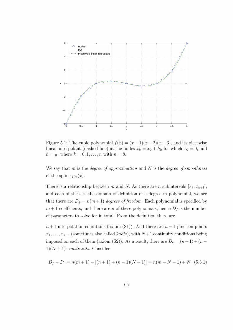
0 0.5 1 1.5 2 2.5 3 3.5 4−6
−4
−2
0
2
4
6
y
x
nodesf(x)Piecewise linear interpolant
Figure 5.1: The cubic polynomial f(x) = (x− 1)(x− 2)(x− 3), and its piecewiselinear interpolant (dashed line) at the nodes xk = x0 + hk for which x0 = 0, andh = 1
2, where k = 0, 1, . . . , n with n = 8.
We say that m is the degree of approximation and N is the degree of smoothness
of the spline pm(x).
There is a relationship between m and N. As there are n subintervals [xk, xk+1],
and each of these is the domain of definition of a degree m polynomial, we see
that there are Df = n(m+1) degrees of freedom. Each polynomial is specified by
m + 1 coefficients, and there are n of these polynomials; hence Df is the number
of parameters to solve for in total. From the definition there are
n + 1 interpolation conditions (axiom (S1)). And there are n− 1 junction points
x1, . . . , xn−1 (sometimes also called knots), with N +1 continuity conditions being
imposed on each of them (axiom (S2)). As a result, there are Dc = (n+1)+(n−1)(N + 1) constraints. Consider
Df −Dc = n(m + 1)− [(n + 1) + (n− 1)(N + 1)] = n(m−N − 1) + N. (5.3.1)
65

It is a common practice to enforce the condition m−N − 1 = 0; that is, we let
m = N + 1. (5.3.2)
This relates the degree of approximation to the degree of smoothness in a simple
manner [10, 11, 37].
66

Example
Figure 5.2 shows the natural and complete cubic spline interpolants to the func-
tion f(x) = e−x2for x ∈ [−1, 1]. We have chosen the nodes xk = −1 + 1
2k, for
k = 0, 1, 2, 3, 4 (i.e., n = 4, and h = 12
). Clearly, f ′(x) = −2xe−x2. Thus, at the
nodes
f(±1) = 0.36787944, f(±1
2) = 0.60653066, f(0) = 1.00000000,
and
f ′(±1) = ∓0.73575888.
−1 −0.8 −0.6 −0.4 −0.2 0 0.2 0.4 0.6 0.8 10.2
0.4
0.6
0.8
1
−1 −0.8 −0.6 −0.4 −0.2 0 0.2 0.4 0.6 0.8 10.2
0.4
0.6
0.8
1
Figure 5.2: Natural and complete (respectively) spline interpolants (dashed lines)for the function f(x) = e−x2
(solid lines) on the interval [−1, 1]. The circlescorrespond to node locations. Here n = 4, with h = 12 , and x0 = −1. Thenodes are at xk = x0 + hk for k = 0, . . . , n.
67

Of course, the spline series for our example has the form
p3(x) =5∑
k=−1
akSk(x),
so we need to determine the coefficients ak. Considering the natural spline inter-
polant first, we have
4 1 0
1 4 1
0 1 4
a1
a2
a3
=
f(x1)− 16f(x0)
f(x2)
f(x3)− 16f(x4)
.
Additionally,
a0 =1
6f(x0) =
1
6f(−1), a4 =
1
6f(x4) =
1
6f(1),
and
a−1 = f(x0)− 4a0 − a1, a5 = f(x4)− 4a4 − a3.
The natural spline series coefficients are therefore
k ak
-1 -0.01094139
0 0.06131324
1 0.13356787
2 0.18321607
3 0.13356787
4 0.06131324
5 -0.01094139
68

Now, on considering the case of the complete spline, we have
4 2 0 0 0
1 4 1 0 0
0 1 4 1 0
0 0 1 4 1
0 0 0 2 4
a0
a1
a2
a3
a4
=
f(x0) + 13hf ′(x0)
f(x1)
f(x2)
f(x3)
f(x4)− 13hf ′(x4)
.
Additionally
a−1 = a1 − 1
3hf ′(x0), a5 = a3 +
1
3hf ′(x4).
The complete spline series coefficients are therefore
k ak
-1 0.01276495
0 0.05493076
1 0.13539143
2 0.18230428
3 0.13539143
4 0.05493076
5 0.01276495
This example demonstrates that the complete spline interpolant tends to be more
accurate than the natural spline interpolant. However, accuracy of the com-
plete spline interpolant is contingent on accurate estimation, or knowledge of the
derivatives f ′(x0) and f ′(xn) [37].
5.3.2 Minimum Mean-Square Error Curve Fitting
Finding a function (curve) y = f(x) that best fits a set of measured x values
and corresponding y values is called curve fitting process.The commonly-used
measure of fit in curve fitting is mean-squared error (MSE). In minimum mean-
squared error (MMSE) curve fitting (also called least-square curve fitting), the
69

parameters of a selected function are chosen to minimize the MSE between the
curve and the measured values.
Polynomial regression is a form of MMSE curve fitting in which the selected
function is a polynomial and the parameters to be chosen are the polynomial
coefficients.
Linear regression is a form of polynomial regression in which the polynomial is
of first degree. The two parameters of a linear equation, representing a straight
line curve, are chosen to minimize the average of the squared distances between
the line and the measured data values [10,22].
Linear Regression
To illustrate linear regression, consider the following set of temperature measure-
ments:
Time (s) Temperature (F )
0 0
1 20
2 60
3 68
4 77
5 110
Observing the plot of these data points shown in Figure 5.3, it can be seen that
a good estimate of a line passing through the points is y = 20x.
A measure of the quality of the fit of the linear estimate to the data is the mean
squared error (MSE ) or the root mean squared error (RMSE )
MSE =1
N
N∑
k=1
(yk − yk)2,
RMSE =√
MSE, (5.3.3)
70
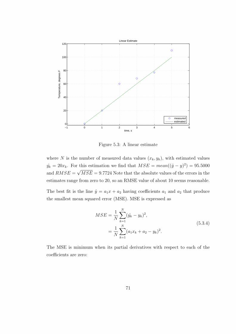
−1 0 1 2 3 4 5 60
20
40
60
80
100
120Linear Estimate
time, s
Tem
pera
ture
, deg
rees
F
measuredestimated
Figure 5.3: A linear estimate
where N is the number of measured data values (xk, yk), with estimated values
yk = 20xk. For this estimation we find that MSE = mean((y − y)2) = 95.5000
and RMSE =√
MSE = 9.7724 Note that the absolute values of the errors in the
estimates range from zero to 20, so an RMSE value of about 10 seems reasonable.
The best fit is the line y = a1x + a2 having coefficients a1 and a2 that produce
the smallest mean squared error (MSE). MSE is expressed as
MSE =1
N
N∑
k=1
(yk − yk)2,
=1
N
N∑
k=1
(a1xk + a2 − yk)2.
(5.3.4)
The MSE is minimum when its partial derivatives with respect to each of the
coefficients are zero:
71
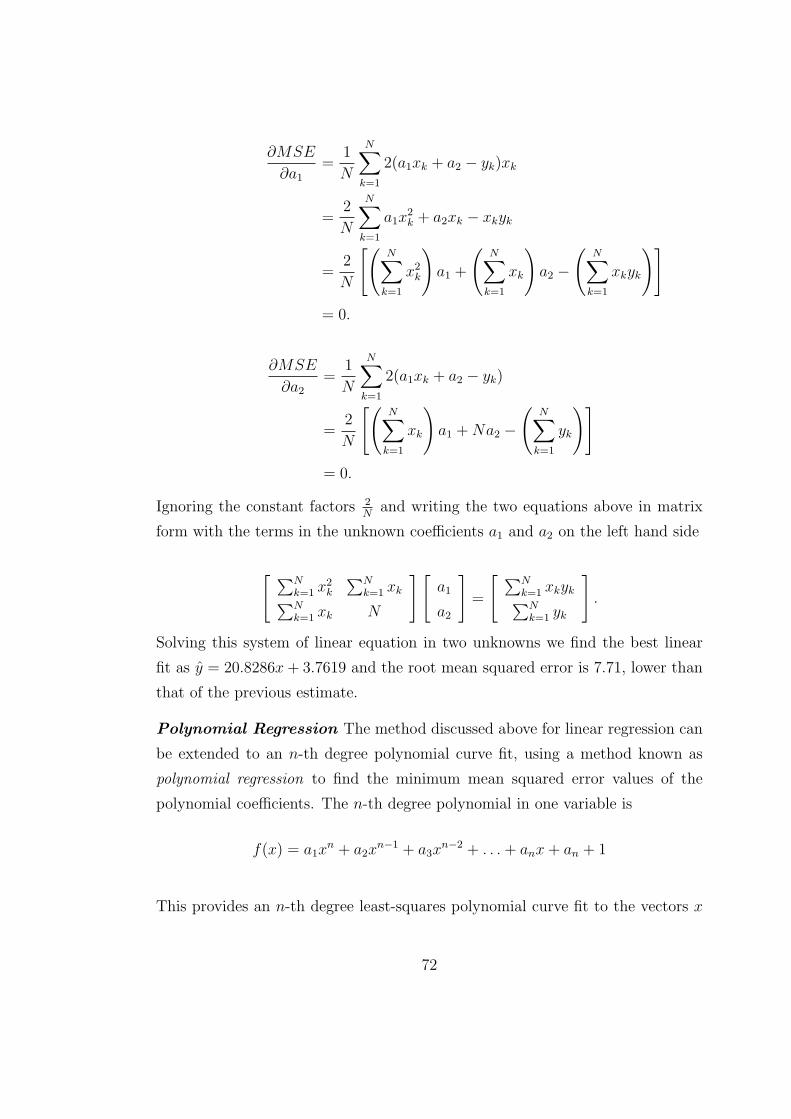
∂MSE
∂a1
=1
N
N∑
k=1
2(a1xk + a2 − yk)xk
=2
N
N∑
k=1
a1x2k + a2xk − xkyk
=2
N
[(N∑
k=1
x2k
)a1 +
(N∑
k=1
xk
)a2 −
(N∑
k=1
xkyk
)]
= 0.
∂MSE
∂a2
=1
N
N∑
k=1
2(a1xk + a2 − yk)
=2
N
[(N∑
k=1
xk
)a1 + Na2 −
(N∑
k=1
yk
)]
= 0.
Ignoring the constant factors 2N
and writing the two equations above in matrix
form with the terms in the unknown coefficients a1 and a2 on the left hand side
[ ∑Nk=1 x2
k
∑Nk=1 xk∑N
k=1 xk N
][a1
a2
]=
[ ∑Nk=1 xkyk∑N
k=1 yk
].
Solving this system of linear equation in two unknowns we find the best linear
fit as y = 20.8286x + 3.7619 and the root mean squared error is 7.71, lower than
that of the previous estimate.
Polynomial Regression The method discussed above for linear regression can
be extended to an n-th degree polynomial curve fit, using a method known as
polynomial regression to find the minimum mean squared error values of the
polynomial coefficients. The n-th degree polynomial in one variable is
f(x) = a1xn + a2x
n−1 + a3xn−2 + . . . + anx + an + 1
This provides an n-th degree least-squares polynomial curve fit to the vectors x
72

and y, which must be of the same length. It returns a coefficient vector a of length
n+1. As the degree increases, the MSE decreases and the number of points that
fall on the curve increases. If a set of n + 1 points is used to determine the n-th
degree polynomial, all n + 1 points will fall on the polynomial curve. Regression
analysis cannot determine a unique solution if the number of points is equal to
or less than the degree of the polynomial model [10, 14, 15].
Theorem 2.2 Least Squares Parabola :
Suppose that {(xk, yk)}Nk=1 are N points where the abscissas are distinct. The
coefficients of the least square parabola
y = f(x) = Ax2 + Bx + C (5.3.5)
are the solution values A, B and C of the linear system
(N∑
k=1
x4k
)A +
(N∑
k=1
x3k
)B +
(N∑
k=1
x2k
)C =
N∑
k=1
ykx2k
(N∑
k=1
x3k
)A +
(N∑
k=1
x2k
)B +
(N∑
k=1
xk
)C =
N∑
k=1
ykxk
(N∑
k=1
x2k
)A +
(N∑
k=1
xk
)B + NC =
N∑
k=1
yk
(5.3.6)
Proof :
The coefficients A, B and C will minimize the quantity
e(A, B, C) =N∑
k=1
(Ax2k + Bxk + C − yk)
2. (5.3.7)
The partial derivatives ∂e∂A
, ∂e∂B
, and ∂e∂C
must all be zero. This results in
73

0 =∂e(A,B,C)
∂A= 2
N∑
k=1
(Ax2k + Bxk + C − yk)
1(x2k)
0 =∂e(A,B,C)
∂B= 2
N∑
k=1
(Ax2k + Bxk + C − yk)
1(xk)
0 =∂e(A,B,C)
∂C= 2
N∑
k=1
(Ax2k + Bxk + C − yk)
1(1)
(5.3.8)
Using the distributive property of addition, we can move the values A,B, and C
outside the summations in (5.3.8) to obtain the normal equations that are given
in (5.3.6).
Example Find the least squares parabola for the four points (−3, 3), (0, 1), (2, 1),
and (4, 3).
The linear system (5.3.6) for finding A, B, and C becomes
353A + 45B + 29C = 79
45A + 29B + 3C = 5
29A + 3B + 4C = 8.
The solution to the linear system is A = 585/3278, B = −631/3278, and C =
1394/1639 and the desired parabola is (see Figure 5.4).
y =585
3278x2 − 631
3278x +
1394
1639= 0.178462x2 − 0.192495x + 0.850519.
5.4 Edge Detection
Over the last decade, various edge detection methods have been applied into
oceanographic satellite images. Although the significant improvements have been
made in edge detection methods, there may be problems when using the algo-
rithms for satellite derived SST images. Due to the degradation and corruption
74
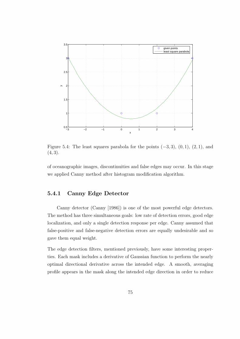
−3 −2 −1 0 1 2 3 40.5
1
1.5
2
2.5
3
3.5
x
y
given pointsleast square parabola
Figure 5.4: The least squares parabola for the points (−3, 3), (0, 1), (2, 1), and(4, 3).
of oceanographic images, discontinuities and false edges may occur. In this stage
we applied Canny method after histogram modification algorithm.
5.4.1 Canny Edge Detector
Canny detector (Canny [1986]) is one of the most powerful edge detectors.
The method has three simultaneous goals: low rate of detection errors, good edge
localization, and only a single detection response per edge. Canny assumed that
false-positive and false-negative detection errors are equally undesirable and so
gave them equal weight.
The edge detection filters, mentioned previously, have some interesting proper-
ties. Each mask includes a derivative of Gaussian function to perform the nearly
optimal directional derivative across the intended edge. A smooth, averaging
profile appears in the mask along the intended edge direction in order to reduce
75
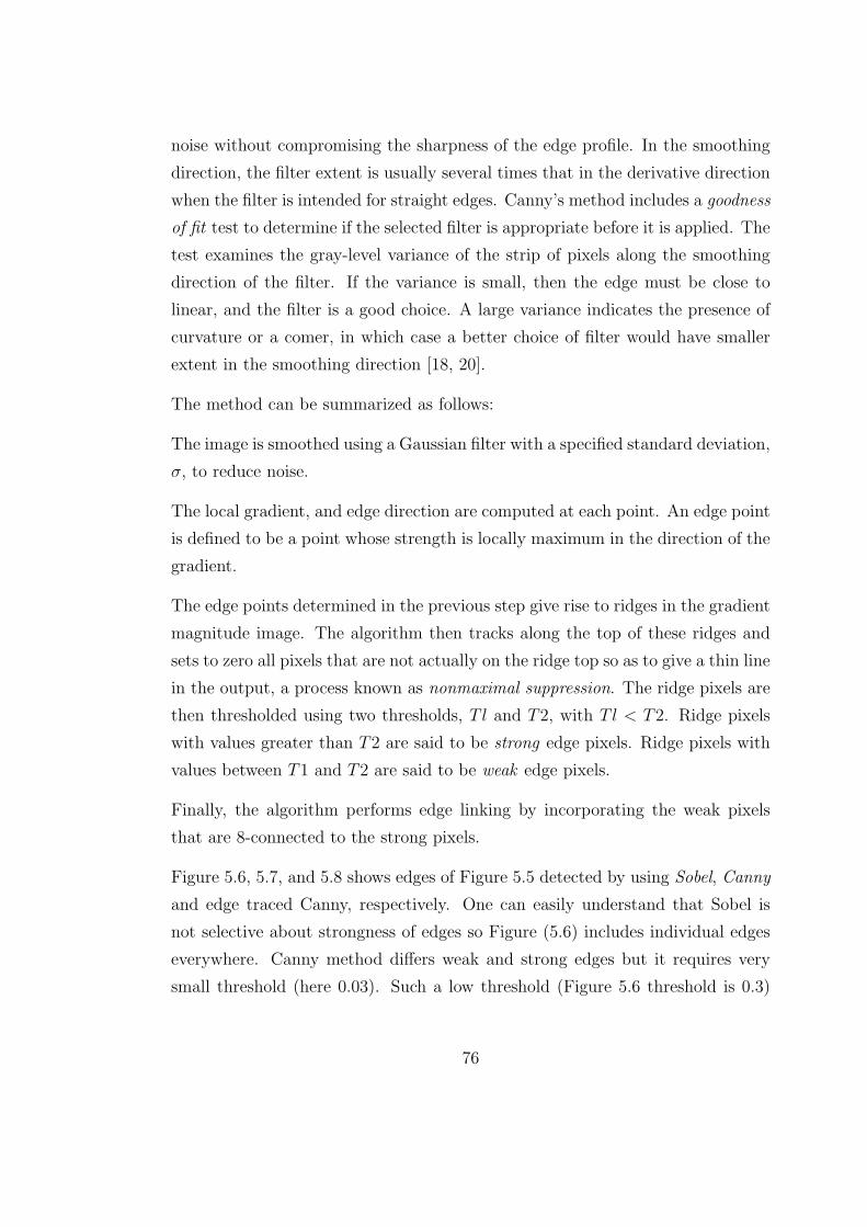
noise without compromising the sharpness of the edge profile. In the smoothing
direction, the filter extent is usually several times that in the derivative direction
when the filter is intended for straight edges. Canny’s method includes a goodness
of fit test to determine if the selected filter is appropriate before it is applied. The
test examines the gray-level variance of the strip of pixels along the smoothing
direction of the filter. If the variance is small, then the edge must be close to
linear, and the filter is a good choice. A large variance indicates the presence of
curvature or a comer, in which case a better choice of filter would have smaller
extent in the smoothing direction [18, 20].
The method can be summarized as follows:
The image is smoothed using a Gaussian filter with a specified standard deviation,
σ, to reduce noise.
The local gradient, and edge direction are computed at each point. An edge point
is defined to be a point whose strength is locally maximum in the direction of the
gradient.
The edge points determined in the previous step give rise to ridges in the gradient
magnitude image. The algorithm then tracks along the top of these ridges and
sets to zero all pixels that are not actually on the ridge top so as to give a thin line
in the output, a process known as nonmaximal suppression. The ridge pixels are
then thresholded using two thresholds, T l and T2, with T l < T2. Ridge pixels
with values greater than T2 are said to be strong edge pixels. Ridge pixels with
values between T1 and T2 are said to be weak edge pixels.
Finally, the algorithm performs edge linking by incorporating the weak pixels
that are 8-connected to the strong pixels.
Figure 5.6, 5.7, and 5.8 shows edges of Figure 5.5 detected by using Sobel, Canny
and edge traced Canny, respectively. One can easily understand that Sobel is
not selective about strongness of edges so Figure (5.6) includes individual edges
everywhere. Canny method differs weak and strong edges but it requires very
small threshold (here 0.03). Such a low threshold (Figure 5.6 threshold is 0.3)
76
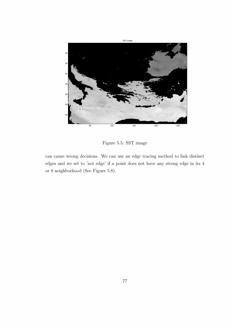
SST image
50 100 150 200 250
50
100
150
200
250
300
350
Figure 5.5: SST image
can cause wrong decisions. We can use an edge tracing method to link distinct
edges and we set to ’not edge’ if a point does not have any strong edge in its 4
or 8 neighborhood (See Figure 5.8).
77
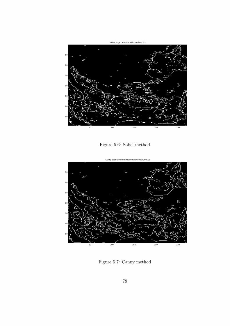
Sobel Edge Detection with threshold 0.3
50 100 150 200 250
50
100
150
200
250
300
350
Figure 5.6: Sobel method
Canny Edge Detection Method with threshold 0.03
50 100 150 200 250
50
100
150
200
250
300
350
Figure 5.7: Canny method
78
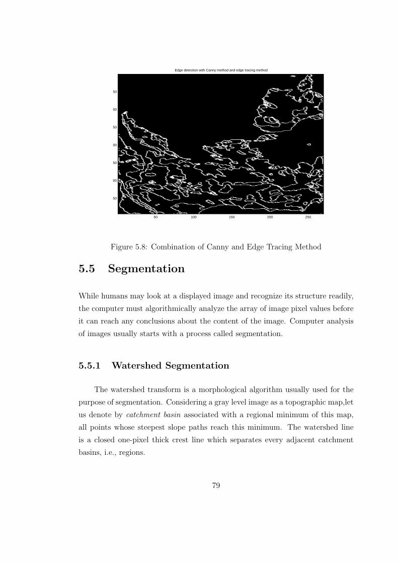
Edge detection with Canny method and edge tracing method
50 100 150 200 250
50
100
150
200
250
300
350
Figure 5.8: Combination of Canny and Edge Tracing Method
5.5 Segmentation
While humans may look at a displayed image and recognize its structure readily,
the computer must algorithmically analyze the array of image pixel values before
it can reach any conclusions about the content of the image. Computer analysis
of images usually starts with a process called segmentation.
5.5.1 Watershed Segmentation
The watershed transform is a morphological algorithm usually used for the
purpose of segmentation. Considering a gray level image as a topographic map,let
us denote by catchment basin associated with a regional minimum of this map,
all points whose steepest slope paths reach this minimum. The watershed line
is a closed one-pixel thick crest line which separates every adjacent catchment
basins, i.e., regions.
79
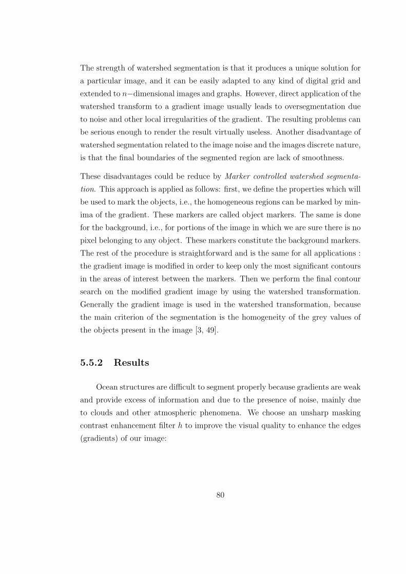
The strength of watershed segmentation is that it produces a unique solution for
a particular image, and it can be easily adapted to any kind of digital grid and
extended to n−dimensional images and graphs. However, direct application of the
watershed transform to a gradient image usually leads to oversegmentation due
to noise and other local irregularities of the gradient. The resulting problems can
be serious enough to render the result virtually useless. Another disadvantage of
watershed segmentation related to the image noise and the images discrete nature,
is that the final boundaries of the segmented region are lack of smoothness.
These disadvantages could be reduce by Marker controlled watershed segmenta-
tion. This approach is applied as follows: first, we define the properties which will
be used to mark the objects, i.e., the homogeneous regions can be marked by min-
ima of the gradient. These markers are called object markers. The same is done
for the background, i.e., for portions of the image in which we are sure there is no
pixel belonging to any object. These markers constitute the background markers.
The rest of the procedure is straightforward and is the same for all applications :
the gradient image is modified in order to keep only the most significant contours
in the areas of interest between the markers. Then we perform the final contour
search on the modified gradient image by using the watershed transformation.
Generally the gradient image is used in the watershed transformation, because
the main criterion of the segmentation is the homogeneity of the grey values of
the objects present in the image [3, 49].
5.5.2 Results
Ocean structures are difficult to segment properly because gradients are weak
and provide excess of information and due to the presence of noise, mainly due
to clouds and other atmospheric phenomena. We choose an unsharp masking
contrast enhancement filter h to improve the visual quality to enhance the edges
(gradients) of our image:
80

h =1
α + 1
−α α− 1 −α
α− 1 α + 5 α− 1
−α α− 1 −α
. (5.5.9)
Due to discontinuities of edge lines, the image do not include concrete objects
and, hence, another operation is necessary for linking these edges. We use an
edge tracing algorithm which depends on the edge direction, and the image is
partitioned into disjointed regions (i.e., segmented) according to these boundaries.
The process searches neighbor pixels until it access the same start point (pixel)
in determined region. If there is no possibility of continuity in any direction the
method fails. Fortunately this situation occurs only if the edges of the objects
have intersection.
Figure (5.9) and (5.10) simply show that watershed segmentation is not ade-
quate for ocean images even if we control oversegmentation/undersegmentation
probability.
5.6 Reconstruction
All of remote sensing sources contain uncertainties which cannot be com-
pletely quantified. Even the most reliable of all available climate data, the instru-
mental records, may contain random, systematic or time-varying biases (Jones et
al. 1999). Due to mechanical problems, out-of-focus blur, motion, inappropriate
illumination, and noise the quality of the digitized image can be inferior to the
original. Image enhancement : In order to aid visual interpretation, the visual
appearance of the objects in the image can be improved by techniques such as
grey level stretching to improve the contrast and spatial filtering for enhancing
the edges. Image restoration or rectification techniques, are intended to correct
for sensor- and platform-specific radiometric and geometric distortions of data.
Radiometric corrections may be necessary due to variations in scene illumination
and viewing geometry, atmospheric conditions, and sensor noise and response. In
81
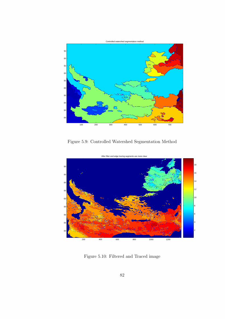
Controlled watershed segmentation method
100 200 300 400 500 600 700
50
100
150
200
250
300
350
400
450
500
Figure 5.9: Controlled Watershed Segmentation Method
After filter and edge tracing segments are more clear
200 400 600 800 1000 1200
200
400
600
800
1000
1200
1400
1600
1800 2
4
6
8
10
12
14
16
18
Figure 5.10: Filtered and Traced image
82
order to actually geometrically correct the original distorted image, a procedure
called resampling is used to determine the digital values to place in the new pixel
locations of the corrected output image. All these techniques aim that make
understandable and clear already available data for last user. However oceano-
graphic images are not completely visible and cloud is the most important reason
of this shortage.
In this thesis, we use only the satellite data with the quality level 0, this quality
level assigned to the data pixels free from any problems that may occur in satellite
data processing due to large solar zenith angles, clouds, sun glint contamination,
shallow water, negative radiance retrievals, failed atmospheric correction. We
approximate an unknown pixel by using the nearest four known pixels’ temper-
ature values without consideration of other parameters such as salinity, height,
etc. These values have inverse rate effect with respect to their distances from
unknown pixel (See Appendix):
sst(i, j) =e
α
(se
e+
sn
n+
sw
w+
ss
s
), (5.6.10)
where sst(i, j) is unknown pixel, s is the distance from nearest south pixel, ss
is the temperature of this pixel, e is the distance from nearest east pixel, se is
the temperature of this pixel, n is the distance from nearest north pixel, sn is
the temperature of this pixel, w is the distance from nearest west pixel, sw is the
temperature of this pixel and α = 1 + en
+ ew
+ es.
Figures 5.12, 5.13 and 5.14 are results of reconstruction of image (see Figure 5.11)
by polynomial fitting, by cubic spline interpolation and by distance based method
explained above. We choose two regions from image and set these regions to
unknown pixels to test our method. One of the regions is chosen less homogeneous
since we can easily realize the methods efficiency.
Number of unknown pixels in the image = 55000.
Number of the finding pixels after reconstruction
polynomial fitting = 48511 in 1m30 seconds,
83
cubic spline interpolation =52123 in 21 seconds,
our technique = 52123 in 2m 17seconds,
rmse (1)= 2,2684,
rmse (2) = 5,78,
rmse (3) = 0.31,
According to rmse (root mean square error) one can think that polynomial fit-
ting gives more reasonable result than cubic spline interpolation but polynomial
fitting is much more sensitive if some pixels are really different than other pixels
and so this may be cause of unacceptable deviation in reconstructed pixel. In
this example one of the missing pixels is evaluated as 31 while actual value is 26
which is a fatal error in SST images. Thus we can only prefer polynomial fit-
ting if data is almost complete but this situation is also so rare in oceanography.
From these results we can say that our technique is more efficient than interpola-
tion techniques but its CPU time is more than others. According to percentage
of unknown pixels (up to 35) our method can be chosen for reconstruction of
oceanographic data.
84

Figure 5.11: Incomplete image
X: 487 Y: 1516Index: 31.23RGB: 0.563, 0, 0
recontruction by polynomial fittin of order 9
200 400 600 800 1000 1200
200
400
600
800
1000
1200
1400
1600
1800
2000
Figure 5.12: Fitting image
85
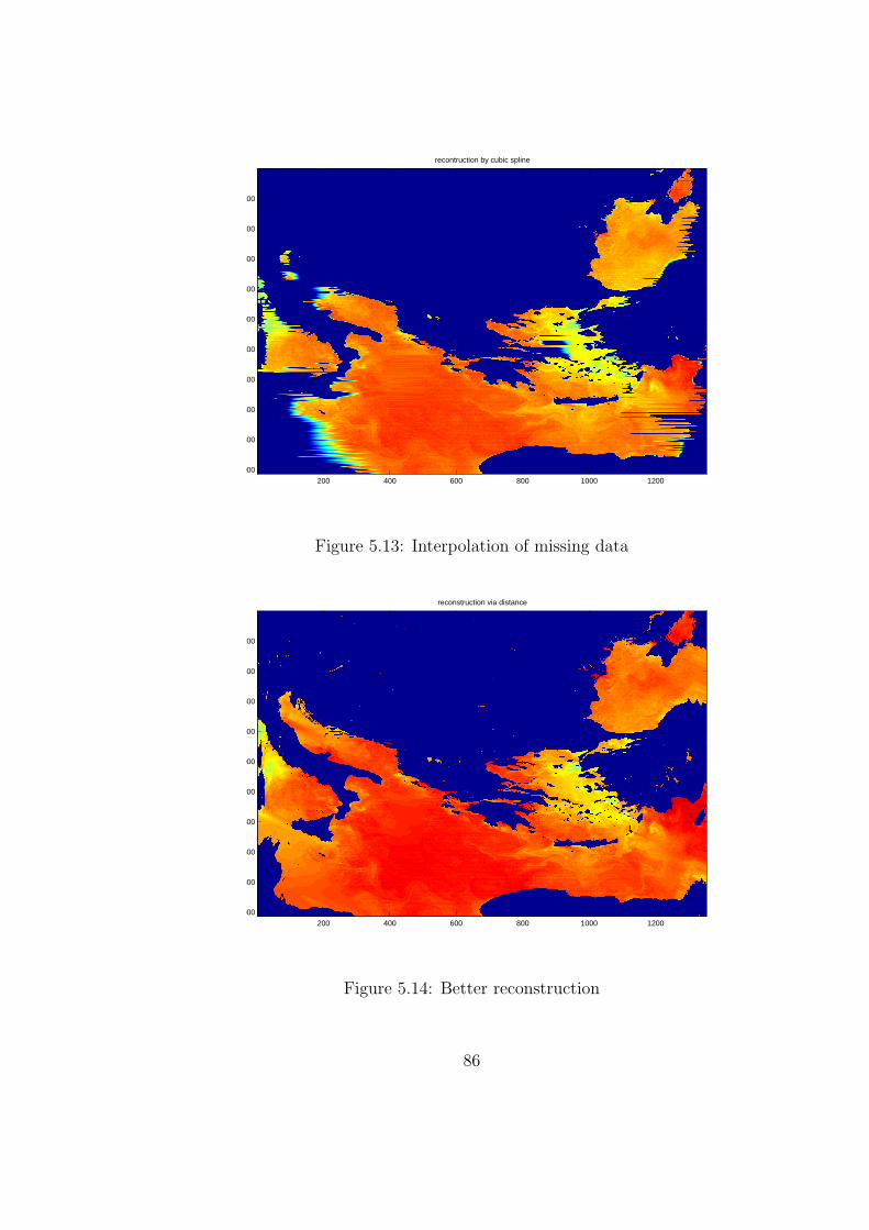
recontruction by cubic spline
200 400 600 800 1000 1200
200
400
600
800
1000
1200
1400
1600
1800
2000
Figure 5.13: Interpolation of missing data
reconstruction via distance
200 400 600 800 1000 1200
200
400
600
800
1000
1200
1400
1600
1800
2000
Figure 5.14: Better reconstruction
86

chapter 6
CONCLUSIONS AND FUTURE
WORK
6.1 Conclusions
Image processing techniques which have convenient results when applied to an
image (e.g., medical, forestry, or photographic) may have inconvenient results
when we apply these techniques to an oceanographic image. This is because
images have different characteristics with respect to belonging area and/or sensor.
Since our data are from MODIS which is more sensitive comparison to other
satellites, and some atmospheric- systematic corrections are done before we get
the data, in addition by the help of quality data we choose quality level 0 to
reduce noise in this data we need not much preprocessing techniques. Thus, in
this study we did not give much place to preprocessing techniques. We can not get
constructive results from other histogram techniques then we applied an adaptive
histogram modification algorithm over our image. (See Figure 6.2)
87
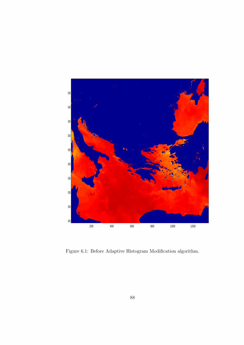
200 400 600 800 1000 1200
200
400
600
800
1000
1200
1400
1600
1800
2000
Figure 6.1: Before Adaptive Histogram Modification algorithm.
88

There are many image segmentation methods in literature generally based on edge
detection, growth of homogeneous regions conditional upon similarities between
pixels or mathematical morphology. Edge based and region based algorithms
performance is insufficient because of deficiencies of SST images. In contrast to
classical segmentation algorithms, the watershed transform has several advan-
tages including the proper handling of gaps and the placement of boundaries at
the most significant edges. But watershed segmentation algorithm requires gra-
dient image and we need another control statement to reduce oversegmentation.
Due to incompleteness of ocean image which we want to segment have approxi-
mate values (even if we reconstruct) so that performance of algorithm decrease.
Most of all, the incompleteness of our data make all the process more difficult.
Thus our main purpose is reconstructing the data. Most of reconstruction (or
estimation) techniques such as interpolation, curve fitting, polynomial fitting give
accurate results when we are dealing with an image less than 10-15 percent miss-
ing pixels. Polynomial fits are unstable in the sense that the values the polyno-
mials give at points between the stations vary greatly for small changes in the
data at the station points, and especially so when data are missing. The problem
gets worse as the order of the polynomial is increased. The method is nearly
useless where the data are sparse. The instability of the polynomial fit is such
that when one key data point is removed, the polynomial fit in that region may
change radically.
Our method find the unknown pixels using known pixels and distances (see Ap-
pendix) but it gives accurate results only if image is not dense. Also CPU time is
not so short and there may be wrong estimates if the values change rapidly. To
understand the efficiency of this algorithm and make comparison look figure and
tables.
We can easily understand that raw data (Figure 6.1) have unqualified data, i.e.
same of the pixels are less than -2 which is an unacceptable situation for oceano-
graphic images. Figure 6.2 we see much gaps since inaccurate pixels (cloud and
nhd) eliminated by using converthdf.m.
89
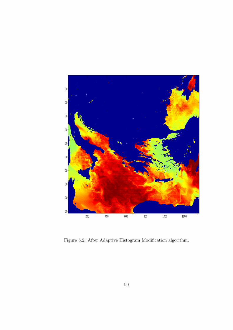
200 400 600 800 1000 1200
200
400
600
800
1000
1200
1400
1600
1800
2000
Figure 6.2: After Adaptive Histogram Modification algorithm.
90
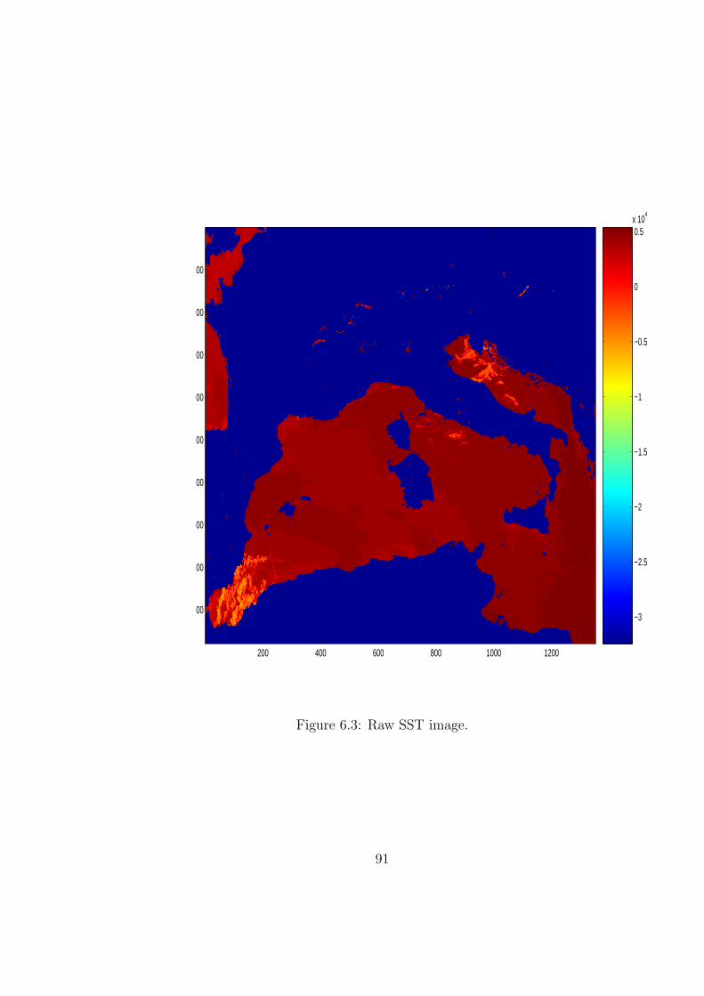
200 400 600 800 1000 1200
200
400
600
800
1000
1200
1400
1600
1800−3
−2.5
−2
−1.5
−1
−0.5
0
0.5x 10
4
Figure 6.3: Raw SST image.
91
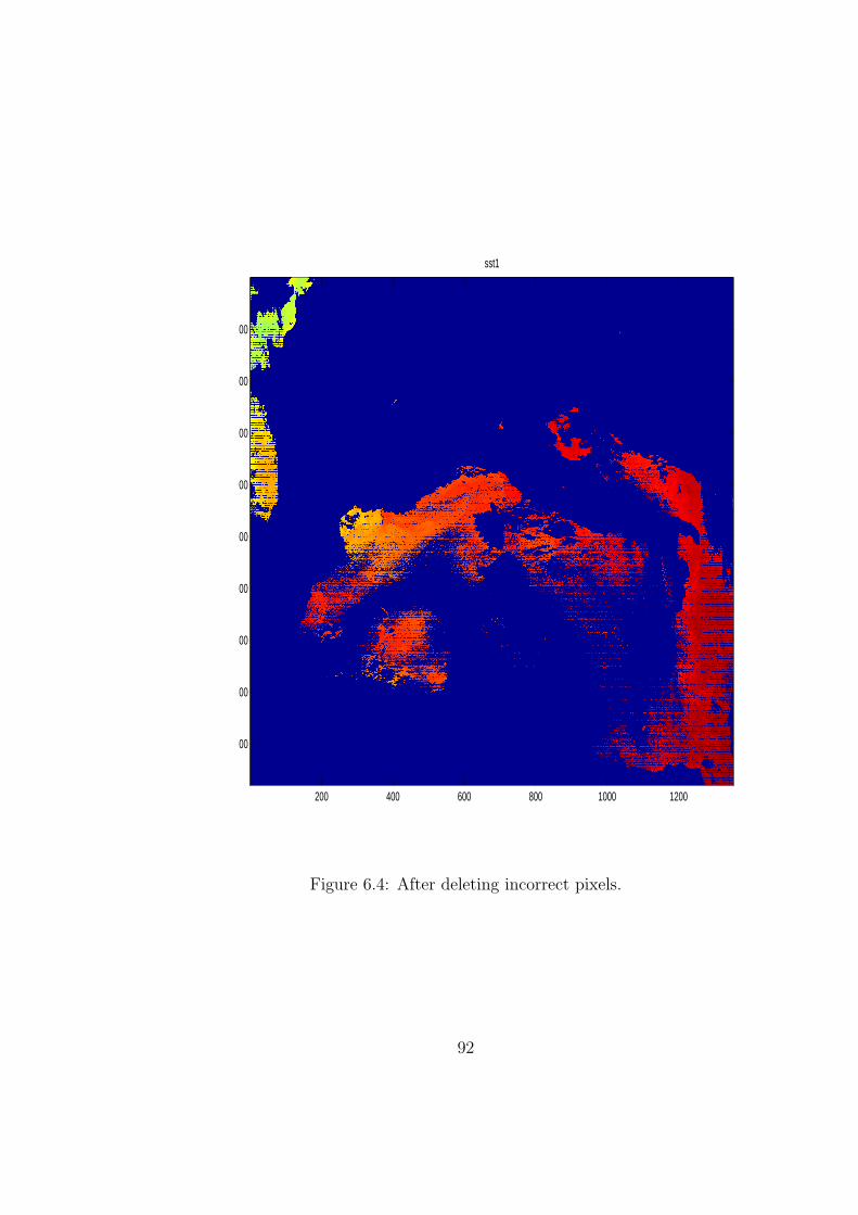
sst1
200 400 600 800 1000 1200
200
400
600
800
1000
1200
1400
1600
1800
Figure 6.4: After deleting incorrect pixels.
92
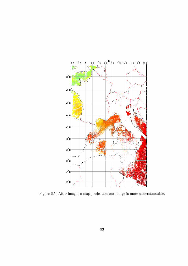
Figure 6.5: After image to map projection our image is more understandable.
93

This data have about %35 inaccuracy (Figure 6.5). In Figure 6.6 below we see
reconstructed image.
Since our data is now complete enough (Figure 6.6), we can try to segment in
more homogenous regions.
94
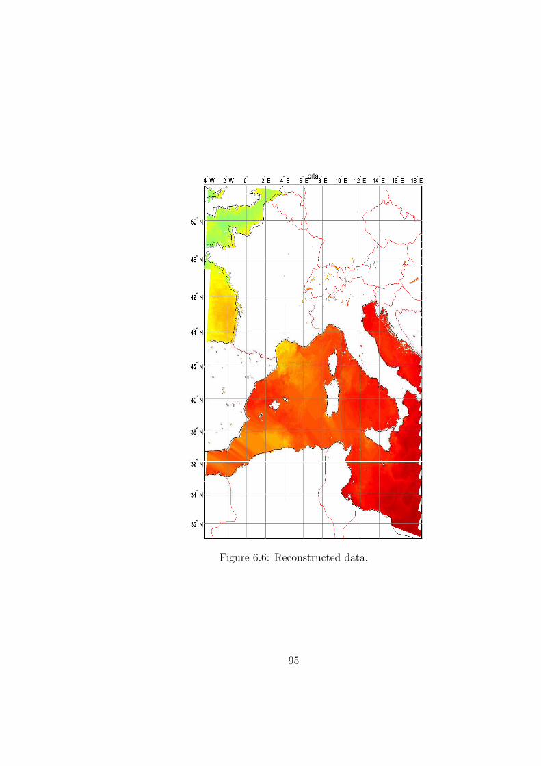
Figure 6.6: Reconstructed data.
95
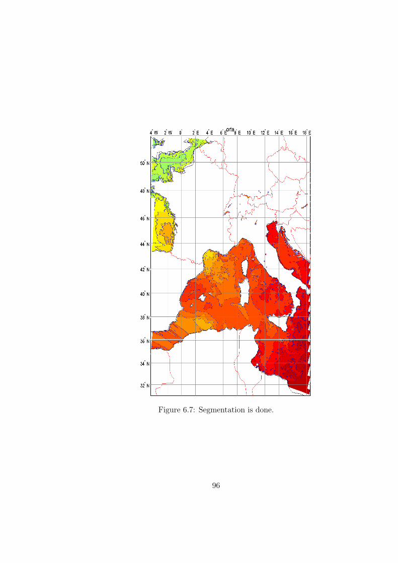
Figure 6.7: Segmentation is done.
96
6.2 Future Work
Satellite sensors provide an alternative approach to measuring SST from ships,
and provide the higher spatial and temporal coverage. So we generate more
capable of characterizing local and seasonal SST changes, over time scales of days
to years and spatial scales of a few kilometers. If used in conjunction with in situ
data, i.e. from ships, moored buoys, the measurements from satellite sensors
become a very powerful tool to understand many oceanographic phenomena.
Despite the undoubted applications of satellite remote sensing techniques to the
study of the sea, it is true to say that for a considerable time the concept of
’oceanography from space’ remained more of a promise than a reality. Sensor
accuracy, cloud cover, and restricted view (little or no information on processes
within the volume of the sea) are some of the reasons.
Besides it is necessary to distinguish between ”bulk” and ”skin” SST. Skin SST is
the radiometric temperature of the sea surface, and refers to the temperature at
the air-sea interface, in a thin layer of the upper microns of the ocean. Bulk SST
refers to the temperature of the upper ocean mixed layer, below the oceanic skin
layer. The bulk SST determined from buoy measurements is typically obtained
at a depth of 1 meter.
The oceans play a key role in regulating the rate of any change in the world’s
climate , which has huge importance present, dedicated ocean satellites are now
required.
As we mentioned before the quality of remote sensing data connected with its
spatial and temporal resolutions. But in reality if a remote sensing system has
high spatial resolution, its temporal resolution is low, and vice versa. So for
better processing it may be useful to merge data (from separate satellites or from
different bands of one sensor).
In this study we used weekly sensed SST images. Due to the fact that reconstruc-
tion algorithm of these images did not depend on time. As we reconstruct of an
97

incomplete image we can not get any idea about unknown pixels by using another
image -from the same satellite- belongs to two weeks ago (or two weeks after).
But one-day data, or fusion of data sensed same day, from different satellites, or
in situ data may used as an approximation about missing data.
Temperature of seawater is dependent primarily upon salinity, depth, density,
wind and pressure. So it is reasonable that estimating SST with the help of other
data such as sea surface height (SSH), sea surface anomaly (SSA).
98

Figure 6.8: Another SST image before reconstruction end segmentation.
99

Figure 6.9: After image processing.
100

references
[1] H. Oktem and Egiazarian, K., A New Histogram Modification Method for
Medical X-Ray Images, (2002).
[2] A.K. Jain, Fundamentals of Digital Image Processing, Prentice Hall, 1989.
[3] A. Pekkarinen, Image segmentation in multisource forest inventory, Finnish
Forest Research Institute, Research Papers 926, 2004.
[4] J. L. Semmlow, Biosignal and Biomedical Image Processing MATLAB-Based
Applications, Marcel Dekker INC., New York, Basel, 2004.
[5] J. Jan, Medical Image Processing Reconstruction and Restoration,Taylor &
Francis Group, Boca Raton London New York Singapore Concepts and
Methods, 2006.
[6] K. Ray and T. Acharya, Image Processing Principles and Applications, John
Wiley & Sons, Inc. 2005.
[7] C. Gonzalez, E. Woods, Digital Image Processing, Second Edition, Prentice
Hall, New Jersey, 2002.
[8] W.K. Pratt, Digital Image Processing, John Wiley & Sons INC., New York,
2001.
[9] J. Berne, Practical handbook on image processing for scientific and technical
applications, 2nd ed., CRC Press, Boca Raton London New York Washing-
ton, D.C., 2004.
101

[10] MATLAB (R14) Help ”MATLAB Function Reference”.
[11] MATLAB Image Processing Toolbox.
[12] J. Serra, Image Analysis and Mathematical Morphology, Academic Press,
New York, 1988.
[13] J. Zarowski, An introduction to Numerical Analysis for Electrical and Com-
puter Engineers, John Wiley & Sons., 2004.
[14] A. Quarteroni, R. Sacco, F. Saleri, Numerical Mathematics, Springer, New
York, 2000.
[15] S. T. Karris, Numerical Analysis Using MATLAB and Spreadsheets, Second
Edition, Orchard publications, U.S.A. 2004.
[16] G. Deng and J. Pinoli, Differentiation-Based Edge Detection Using the Log-
arithmic Image Processing Model, Journal of Mathematical Imaging and Vi-
sion 8, 161-180 (1998).
[17] J. Starck and F. Murtagh, Handbook of Astronomical Data Analysis,
Springer, Verlag, 2000.
[18] D. Phillips, Image Processing in C, R D Publications, Kansas, 2000.
[19] (eBook) - Mathematics - Math Problems Solving With Matlab Programming.
[20] J. L. Schafer, Analysis Of Incomplete Multivariate Data, CRC Press,
NewYork Washington 2000.
102

[21] W. Collins, Fundamental Numerical Methods and Data Analysis, Second
Edition, 2003.
[22] W. Y. Yang, Applied Numerical Methods Using Matlab., A John Wiley &
Sons, 2005.
[23] G. P. Brasseur, J. J. Orlando, and G. S. Tyndall, Atmospheric chemistry
and global change, 1. ed., Oxford University Press, New York, 1999.
[24] K. Levenberg, A method fo the solution of certain problems in least-squares,
Quarterly Applied Math., 2, 164–168, 1944.
[25] W. G. Rees, Physical Principles of Remote Sensing, Second Edition, Cam-
bridge University Press, 2001.
[26] R.M. Lewitt, Reconstruction algorithms: Transform methods, Proc. IEEE,
vol. 71, pp. 390–408, March 1983.
[27] D. Early and D.G. Long, Image reconstruction and enhanced resolution imag-
ing from irregular samples, submitted to TGARRS, 2000.
[28] S.F. Gull and G.J. Daniell, Image reconstruction from incomplete and noisy
data, Nature, 1978.
[29] R.L. Lagendijk and J. Biemond, Iterative Identification and Restoration of
Images, Kluver Academic Publishers, 1991.
[30] D.E. Myers , Interpolation and estimation with spatially located data, Chemo-
metrics and Intelligent Laboratory Systems, 11, 209–228, 1991.
103
[31] D. Anding and R. Kauth, Estimation of sea surface temperature from space,
Remote Sens. Environ., Vol. 1, pp. 217–220, 1970.
[32] W. L. Barnes, T. Pagano, and V. V. Salomonson, Prelaunch characteristics
of the Moderate Resolution Imaging Spectroradiometer (MODIS), 1998.
[33] I. J. Barton, M. Zavody, D. M. OBrien, D. R. Cutten, R. W. Saunders, and
D. T. Llewellyn-Jones, Theoretical algorithms for satellite-derived sea surface
temperatures, J. Geophys. Res., vol. 94, p. 3365, 1989.
[34] H. R. Gordon, Removal of atmospheric effects from satellite imagery of the
oceans, Appl. Opt., Vol. 17, pp. 1631–1636 ,1978.
[35] H. R. Gordon, T. Du, and T. Zhang, Remote sensing ocean color and aerosol
properties: resolving the issue of aerosol absorption, Appl. Opt., 1997.
[36] F. Bryan and D. Thomas, Overview of MODIS/Aqua Ocean Color Processing
& Distribution, May 2005.
[37] G. Aubert and P.Kornprobst, Mathematical Problems in Image Processing,
Springer, New York, 2000.
[38] J. Besag, On the statistical analysis of dirty pictures, Journal of the Royal
Statistical Society, 48(3): 259–302, 1986.
[39] F. C. Tonyand and A. V. Luminita, Active contours without edges, IEEE
Trans. on Image Proc., 10(2): 266–277, February 2001.
[40] W. Feller, An Introduction to Probability Theory and Its Applications, Vol-
ume II. John Wiley & Sons, Inc., 2 edition, 1966.
104

[41] A. Nagy, A. Kuba, and M. Samal, Reconstruction of factor structures using
discrete tomography method, Electronic Notes in Discrete Mathematics, 20:
519–534, 2005.
[42] Y. Rubner, C. Tomasi, and J. Guibas, The earth movers distance as a metric
for image retrieval, International Journal of Computer Vision, 40(2) :99–121,
2000.
[43] P. Simoncelli, Statistical models for images: Compression, restoration and
synthesis, In 31st Asilomar Conf. on Signals, Systems, and Computers, Pa-
cific Grove, CA IEEE Sig. Proc. Soc., 1997.
[44] J. Shi and J. Malik, Normalized cuts and image segmentation, IEEE Trans.
Patt. Anal. Mach. Intell., 22(8): 888–905, 2000.
[45] I. T. Young, J. Gerbrands, and J. van Vliet, Fundamentals of Image Pro-
cessing, Netherlands, 1995.
[46] Fundamentals of Remote Sensing, Remote Sensing Tutorial,
Canada Centre for Remote Sensing, Natural Resources, Canada
http://www.ccrs.nrcan.gc.ca/ccrs
[47] T. M. Lillesand and R. W. Kiefer, Remote Sensing and Image Interpretation,
University of Wisconsin, John Wiley & Sons, 2000.
[48] E. Green, P. Mumby, A. Edwards, and C. Clark, Remote Sensing Hand-
book for Tropical Coastal Management, Coastal Management Sourcebooks
3, UNESCO, Paris, 2000.
[49] F. Meyer and S. Boucher , Morphological Segmentation”. Journal of Visual
Communication and Image representation, Academic Press, 1990.
105

[50] J. R. Jensen, Introductory Digital Image Processing: A Remote Sensing Per-
spective, Prentice Hall, New Jersey, 1996.
[51] A. Bovik, Handbook of Image and Video Processing, Academic Press, New
York ,Boston, 2000.
[52] A. Ardeshir Goshtasby, 2-D and 3-D Image Registration for Medical, Remote
Sensing, and Industrial Applications, John Wiley & Sons, 2005.
http://oceancolor.gsfc.nasa.gov/DOCS.
http://oceancolor.gsfc.nasa.gov/PRODUCTS/.
http://oceancolor.gsfc.nasa.gov/DOCS/MSL12/.
http://oceancolor.gsfc.nasa.gov/DOCS/MSL12/CODE/.
MODIS Algorithm Theoretical Basis Document: MOD17, MOD25, MOD28.
106

Appendix A
MATLAB Code for Conversion of HDF
% (C) Muserref TURKMEN
% This algorithm convert hdf file to matrix
%( size = number of scan lines * pixel per scan line)
hdfile = ’A2002203012500.L2-LAC-SST.x.hdf’
hInfo = hdfinfo(hdfile);
myfile=hInfo.Filename;
namequal-sst=hInfo.Vgroup(1,2).SDS(1,2).Name;
aqual-sst=hInfo.Vgroup(1,2).SDS(1,2).Dims(1,1).Size;
bqual-sst=hInfo.Vgroup(1,2).SDS(1,2).Dims(2,1).Size;
qual-sst = hdfread(myfile,namequal-sst,’Index’, [1.0 1.0 ],[1.0 1.0 ],[aqual-sst bqual-
sst ]);
namesst=hInfo.Vgroup(1,2).SDS(1,1).Name;
asst=hInfo.Vgroup(1,2).SDS(1,1).Dims(1,1).Size;
bsst=hInfo.Vgroup(1,2).SDS(1,1).Dims(2,1).Size;
sst = hdfread(myfile,namesst,’Index’, [1.0 1.0 ],[1.0 1.0 ],[asst bsst ]);
namel2flags=hInfo.Vgroup(1,2).SDS(1,3).Name;
al2flag=hInfo.Vgroup(1,2).SDS(1,3).Dims(1,1).Size;
bl2flag=hInfo.Vgroup(1,2).SDS(1,3).Dims(2,1).Size;
l2-flags = hdfread(myfile,namel2flags,’Index’, [1.0 1.0 ],[1.0 1.0 ],[al2flag bl2flag
]);
107

namelon=hInfo.Vgroup(1,3).SDS(1,1).Name;
alon=hInfo.Vgroup(1,3).SDS(1,1).Dims(1,1).Size;
blon=hInfo.Vgroup(1,3).SDS(1,1).Dims(2,1).Size;
longitude = hdfread(myfile,namelon,’Index’, [1.0 1.0 ],[1.0 1.0 ],[alon blon ]);
namelat=hInfo.Vgroup(1,3).SDS(1,2).Name;
alat=hInfo.Vgroup(1,3).SDS(1,2).Dims(1,1).Size;
blat=hInfo.Vgroup(1,3).SDS(1,2).Dims(2,1).Size;
latitude = hdfread(myfile,namelat,’Index’, [1.0 1.0 ],[1.0 1.0 ],[alat blat ]);
latitude=imresize(double(latitude),.1);
longitude=imresize(double(longitude),.1);
maplat2=double(hInfo.Attributes(1,28).Value);
maplat1=double(hInfo.Attributes(1,46).Value);
maplon1=double(hInfo.Attributes(1,26).Value);
maplon2=double(hInfo.Attributes(1,44).Value);
sst=double(sst);
%we eliminate unqualified pixels
sst1=sst;
qual-sst=double(qual-sst);
maxqual=max(max(qual-sst));
for i=1:size(qual-sst,1)
for j=1:size(qual-sst,2)
if qual-sst(i,j)==maxqual-1 — qual-sst(i,j)==maxqual
108
sst(i,j)=NaN;
if sst1(i,j)¡=-32760
sst(i,j)=0;
end
end
end
end
%slope = 0.0049999999f ;intercept = 0.f ;
%to convert a 16 bit [-32768 ,32767] pixel value to 0C
sst=0.005*sst;
% we calculate the percentage of incomplete data. (about % 20 is OK)
cii=0;
cnan=0;
for i=1:size(sst,1);
for j=1:size(sst,2)
if isnan(sst(i,j))
cnan=cnan+1;
elseif sst(i,j)¿0
cii=cii+1;
end
end
end
109

accu=(100*cnan)/(i*j)
%image to map projection
mercatorm(sst,maplat2,maplat1,maplon1,maplon2,latitude,longitude);
110

MATLAB Code for Histogram Modification
% (C) Hakan OKTEM
% Adaptive Histogram Modification algorithm.
function [oupt,outt]=adtstr(img,itop,ibot,ilef,irig,sfvl,clipsize,gamm,nofbins,sensiv);
%itop,ibot,ilef,irig = offsets they are for preventing the effect of the
%sides of the image with too much noise for a 2024x2024 image taking all
%around 50 is OK
%sfvl = will be added to input data histogram. 2-3 is generally appropriate
%if there are not big gaps in the histogram it can be taken 0
%clipsize = legth of the clipping window to remove the outliers 3 is an
%appropriate choice
%gamm= constant for span adjustment. Main parameter. 0 ¡ gamm ¡ 1. I was
setting it by trial and error
%nofbins= number of the bins in the histogram generally 256 but can be
%increased if better accuracy is desired
%calculate the size of the image and selected portion
[aa,bb]=size(img);
usm=itop+1;
alm=aa-ibot;
slm=ilef+1;
sgm=bb-irig;
%normalize the image
111

img=double(img);
img=img-min(min(img));
img=img/max(max(max(img)),2*eps);
%clip the data
%find min of local maxes and max of local mins
%this is necessary for eliminating the effects of extreme values
%which may occur due to the scattering of x-ray photons of limited dose
minofmax=1;
maxofmin=0;
for i=1:clipsize:aa-clipsize,
for j=1:clipsize:bb-clipsize,
minofmax=min(minofmax,max(max(img(i:i-1+clipsize,j:j-1+clipsize))));
maxofmin=max(maxofmin,min(min(img(i:i-1+clipsize,j:j-1+clipsize))));
end
end
%make clipping
img=max(img,minofmax);
img=min(img,maxofmin);
%normalize
img=img-min(min(img));
img=img/max(max(max(img)),2*eps);
%compute the input histogram
112

hgrm=himhist(img(usm:alm,slm:sgm),nofbins);
%add sfvl to conserve the real differences partially
hgrm=hgrm+sfvl;
%find the mins and maxes of the selected window
immin=min(min(img(usm:alm,slm:sgm)));
immax=max(max(max(img(usm:alm,slm:sgm))),2*eps);
%calculate the span for distributing the selected portion data
oupmin=gamm*immin;
oupmax=1-((1-immax)*gamm);
inrang=immax-immin;
ourang=oupmax-oupmin;
%perform the desired point transformation
totl=sum(sum(hgrm));
oupt=(oupmin/max(immin,2*eps))*min(img,immin);
for i=1:nofbins,
oupt=oupt+((ourang/max(inrang,2*eps))*(hgrm(i)/totl)*nofbins*min(img-(((i-1)*inrang)/nofbins)-
immin,(inrang/nofbins)).*(img¿((((i-1)*inrang)/nofbins)+immin)));
end
oupt=oupt+((1-oupmax)/max(1-immax,2*eps))*(img-immax).*(img¿immax);
%normalize
oupt=oupt-min(min(oupt));
oupt=oupt/max(max(max(oupt)),2*eps);
113

% the selected area based histogram flattening is completed up to here % after
here ”% %” is the comment line and % is for the code lines using unavailable
data
% % histogram mapping stage
% load trgt;
hgrm=hgrm-sfvl;
totl=sum(sum(hgrm));
avrg=totl/nofbins;
trggt=hgrm.*(hgrm¿(avrg*sensiv));
nwsiz=sum(hgrm¿(avrg*sensiv));
trgt=zeros([nwsiz,1]);
inds=1;
% % read the target histogram to the array ”trgt”. ”trgt.mat” is assumed to
have the desired histogram which is not available yet
for i=1:nofbins,
if trggt(i)¿0.5,
trgt(inds)=trggt(i);
inds=inds+1;
end
end
trgtot=sum(trgt);
outt=min(oupt,oupmin);
lvv=oupmin;
114

for i=1:nwsiz,
outt=outt+(trgtot/(trgt(i)*nwsiz))*min(oupt-lvv,trgt(i)*ourang/trgtot).*(oupt¿lvv);
lvv=lvv+trgt(i)*ourang/trgtot;
end
outt=outt+(oupt-oupmax).*(oupt¿oupmax);
outt=outt-min(min(outt));
outt=outt/max(max(max(outt)),2*eps);
115

MATLAB Code for Reconstruction
% this algorithm finds unknown pixels of incomplete SST image
% This algorithm is called in converthdf.m so we do not write parameters again.
for i=2:size(sst,1)
for j=2:size(sst,2)
if isnan(sst(i,j))
count=0;
count1=0;
count2=0;
count3=0;
count4=0;
value=0;
iminusa1=0;
iplusa2=0;
jminusb1=0;
jplusb2=0;
%we try to figure out known pixels at the same row or column with missing pixel
for a=i-1:-1:1
% in this stage we eliminate pixels wrt distance between missing pixel
%we start from the most northest, westest, eastest and southest pixels
%our aim is to find nearest pixel in the direction.
% we research for all 4 direction if isnan(sst(i-a,j)) & sst(i-a,j)¿0
116

count=1;
count1=1;
iminusa1=sst(i-a,j);
x1=a;
end
end
for b=j-1:-1:1
if isnan(sst(i,j-b)) & sst(i,j-b)¿0
count2=1;
if count1==0
count=1;
else
count=2;
end
jminusb1=sst(i,j-b);
y1=b;
end
end
for a=size(sst,1)-i:-1:1
if isnan(sst(i+a,j)) & sst(i+a,j)¿0
count3=1;
if count1+count2==2
117
count=3;
elseif count1+count2==1
count=2;
else
count=1;
end
iplusa2=sst(i+a,j);
x2=a;
end
end
for b=size(sst,2)-j:-1:1
if isnan(sst(i,j+b)) & sst(i,j+b)¿0
count4=1;
if count1+count2+count3==3
count=4;
elseif count1+count2+count3==2
count=3;
elseif count1+count2+count3==1
count=2;
else
count=1;
end
118

jplusb2=sst(i,j+b);
y2=b; end
end
% we approximate the missing pixel using known pixels...
% count is the number of known pixel.
% we search only 4 direction, (countmax = 4)
if count==4
alpha=1+x1/x2+x1/y1+x1/y2;
sst(i,j)=(x1/alpha)*(iminusa1*1/x1+iplusa2*1/x2+jminusb1*1/y1+jplusb2*1/y2);
elseif count==3 & jminusb1==0
alpha=1+x1/x2+x1/y2;
sst(i,j)=(x1/alpha)*(iminusa1*1/x1+iplusa2*1/x2+jplusb2*1/y2);
elseif count==3 & iplusa2==0
alpha=1+x1/y1+x1/y2;
sst(i,j)=(x1/alpha)*(iminusa1*1/x1+jminusb1*1/y1+jplusb2*1/y2);
elseif count==3 & jplusb2==0
alpha=1+x1/x2+x1/y1;
sst(i,j)=(x1/alpha)*(iminusa1*1/x1+iplusa2*1/x2+jminusb1*1/y1);
elseif count==3 & iminusa1==0
alpha=1+x2/y1+x2/y2;
sst(i,j)=(x2/alpha)*(iplusa2*1/x2+jminusb1*1/y1+jplusb2*1/y2);
elseif count==2 & iminusa1==0
119

if iplusa2==0
alpha=1+y1/y2;
sst(i,j)=(y1/alpha)*(jminusb1*1/y1+jplusb2*1/y2);
elseif jminusb1==0
alpha=1+x2/y2;
sst(i,j)=(x2/alpha)*(iplusa2*1/x2+jplusb2*1/y2);
elseif jplusb2==0
alpha=1+x2/y1;
sst(i,j)=(x2/alpha)*(iplusa2*1/x2+jminusb1*1/y1);
end
elseif count==2 & iplusa2==0
if jminusb1==0
alpha=1+x1/y2;
sst(i,j)=(x1/alpha)*(iminusa1*1/x1+jplusb2*1/y2);
elseif jplusb2==0
alpha=1+x1/y1;
sst(i,j)=(x1/alpha)*(iminusa1*1/x1+jminusb1*1/y1);
end
elseif count==2 & jminusb1==0
if jplusb2==0
alpha=1+x1/x2;
sst(i,j)=(x1/alpha)*(iminusa1*1/x1+iplusa2*1/x2);
120

end
end
end
end
end
121

Appendix B
Properties of data:
Name: A2007099002500.L2-LAC-SST.x.hdf
Title: MODISA Level-2 Data
Sensor Name: MODISA
Product Name: A2007099002500.L2-LAC-SST
Software Name: MSl12 (name of the software used to create this product.)
Software Version: 5.6.5 (version of the software used to create this product.)
Replacement Flag: ORIGINAL
Orbit Node Longitude: 0 (longitude at equatorial crossing of day-side node).
Orbit Number: 0 (orbit number of the scene.)
Node Crossing Time:
Processing Time: 2007107052624000 local time of generation of this product;
concatenated digits for year, day-of-year, hours, minutes, seconds, and fraction
of seconds in the format of YYYYDDDHHMMSSFFF.
Creation Time: 2007117210812000
Processing Control: MSl12 (path and name of the file containing the control
parameters. This information is stored in the product as part of its processing
history.)
par=/data1/vdc/sdpsoper/vpu0/workbuf/A2007099002500.L1B-LAC.param
metafile=A2007099002500.L2-LAC.meta
Input Parameters:
IFILE1 = /data1/vdc/sdpsoper/vpu0/workbuf/A2007099002500.L1B-LAC
122

OFILE1 = A2007099002500.L2-LAC-SST
L2PROD1 = sst, qual-sst, l2-flags
CALFILE = CLDFILE = GEOFILE =/data1/vdc/sdpsoper/vpu0/workbuf/A2007099002500.
GEO RFLAG = ORIGINAL
EVAL = 0
MODE = 0
SPIXL = 1
EPIXL = -1
DPIXL = 1
SLINE = 1
ELINE = -1
DLINE = 1
CTL-PT-INCR = 8
PROC-OCEAN = 1
PROC-LAND = 0
ATMOCOR = 1
AER-OPT = -3
AER-WAVE-SHORT = 748
AER-WAVE-LONG = 869
AER-SWIR-SHORT = -1
AER-SWIR-LONG = -1
AER-ITER-MAX = 10
123
BRDF-OPT = 7
GAS-OPT = 1
IOP-OPT = 0
GSM01-OPT = 0
GSM01-FIT = 0
QAA-OPT = 0
QAA-S = 0.01500
POL-OPT = 3
ABSAER-OPT = 0
SL-PIXL = -1
SL-FRAC = 0.2500
GLINT-OPT = 1
RESOLUTION = -1
OUTBAND-OPT = 2
OXABAND-OPT = 0
FILTER-OPT = 1
FILTER-FILE = /sdps/sdpsoper/data/OCDATA/data/modisa/msl12-filter.dat
FILTER-1 = 7 x 5 (1) straylight filter on flag 5
FILTER-2 = 7 x 5 (1) straylight filter on flag 10
MET1 = /data1/vdc/sdpsoper/vpu0/workbuf/S200709900-NCEP.MET
MET2 = /data1/vdc/sdpsoper/vpu0/workbuf/S200709906-NCEP.MET
MET3 = /data1/vdc/sdpsoper/vpu0/workbuf/S200709906-NCEP.MET
124

OZONE1 = /data1/vdc/sdpsoper/vpu0/workbuf/S20070980009823-TOAST.OZONE
OZONE2 = /data1/vdc/sdpsoper/vpu0/workbuf/S20070990009923-TOAST.OZONE
OZONE3 = /data1/vdc/sdpsoper/vpu0/workbuf/S20070990009923-TOAST.OZONE
LAND = /sdps/sdpsoper/data/OCDATA/data/common/landmask.dat
WATER = /sdps/sdpsoper/data/OCDATA/data/common/watermask.dat
DEMFILE = /sdps/sdpsoper/data/OCDATA/data/common/digital-elevation-map.hdf
ICEFILE = /sdps/sdpsoper/data/OCDATA/data/common/ice-mask.hdf
SSTFILE = /data1/vdc/sdpsoper/vpu0/workbuf/oisst.20070411
NO2FILE = /sdps/sdpsoper/data/OCDATA/data/common/no2-climatology.hdf
ALPHAFILE = /sdps/sdpsoper/data/OCDATA/data/common/alpha510-climatology.hdf
TAUAFILE = /sdps/sdpsoper/data/OCDATA/data/common/taua865-climatology.hdf
GAIN = 0.9710, 0.9848, 0.9795, 0.9870, 0.9850, 0.9797, 0.9776, 0.9855, 1.0000
OFFSET = 0.00000, 0.00000, 0.00000, 0.00000, 0.00000, 0.00000, 0.00000, 0.00000,
0.00000
AERMODELS = o99, m50, m70, m90, m99, c50, c70, c90, c99, t50, t90, t99
TAUA = 0.0000, 0.0000, 0.0000, 0.0000, 0.0000, 0.0000, 0.0000, 0.0000, 0.0000
AERMODRAT = 0.00000
AERMODMIN = -1f
AERMODMAX = -1f
ALBEDO = 0.027
ABSAER = 0.000
RHOAMIN = 0.00010
125

NLWMIN = 0.150
HIPOL = 0.500
WSMAX = 8.000
TAUAMAX = 0.300
EPSMIN = 0.850
EPSMAX = 1.350
GLINT-THRESH = 0.005
WINDSPEED = -1000.000
WINDANGLE = -1000.000
PRESSURE = -1000.000
OZONE = -1000.000
WATERVAPOR = -1000.000
RELHUMID = -1000.000
SUNZEN = 90.000
SATZEN = 60.000
MASKLAND = 1
MASKBATH = 0
MASKCLOUD = 1
MASKGLINT = 0
MASKSUNZEN = 0
MASKSATZEN = 0
MASKHILT = 1
126
MASKSTLIGHT = 0
MUMM-ALPHA = 1.945
MUMM-GAMMA = 1.000
MUMM-EPSILON = 1.000
CHLOC2-WAVE = -1, -1
CHLOC2-COEF = 0.00000, 0.00000, 0.00000, 0.00000, 0.00000
CHLOC3-WAVE = 443, 489, 550
CHLOC3-COEF = 0.28300, -2.75300, 1.45700, 0.65900, -1.40300
CHLOC4-WAVE = -1, -1, -1, -1
CHLOC4-COEF = 0.00000, 0.00000, 0.00000, 0.00000, 0.00000
CHLCLARK-WAVE = 443, 488, 551
CHLCLARK-COEF = 0.78927, -3.92552, 11.63776, -27.15800, 27.93696, -10.39859
VCAL-OPT = -1
VCAL-NLW = 0.0000, 0.0000, 0.0000, 0.0000, 0.0000, 0.0000, 0.0000, 0.0000,
0.0000
VCAL-LW = 0.0000, 0.0000, 0.0000, 0.0000, 0.0000, 0.0000, 0.0000, 0.0000, 0.0000
VCAL-CHL = -1.0000
VCAL-SOLZ = -1.0000
Input Files: (the names of the Level-1A or Level-1B file from which the current
product was created and of the ancillary (environmental) data files used in the
processing. This information is stored in the product as part of its processing
history.)
A2007099002500.L1B-LAC,S200709900-NCEP.MET,
127

S200709906-NCEP.MET,S200709906-NCEP.MET,
S20070980009823-TOAST.OZONE,
S20070990009923-TOAST.OZONE,
S20070990009923-TOAST.OZONE,,,
landmask.dat,
watermask.dat,
digital-elevation-map.hdf,
ice-mask.hdf,
oisst.20070411,
no2-climatology.hdf,
alpha510-climatology.hdf,
taua865-climatology.hdf,
A2007099002500.GEO,
Mask Names: ATMFAIL, LAND, CLDICE, HILT
Number of Bands: 9
Number of Scan Lines: 1972
Pixels per Scan Line: 1354
Scene Center Scan Line: 987
Number of Scan Control Points: 1972
Number of Pixel Control Points: 1354
Start Time: 2007099002515394
Start Year: 2007
128

Start Day: 99
Start Millisec: 1515395
Upper Left Longitude: 10.9751
Upper Right Longitude: 41.9633
Upper Left Latitude: 50.3737
Upper Right Latitude: 45.8908
Start Center Longitude: 27.2085
Start Center Latitude: 49.2052
Latitude Units: degrees North
Longitude Units: degrees East
Scene Center Time: 2007099002741628
Scene Center Longitude: 24.0747
Scene Center Latitude: 40.5351
Scene Center Solar Zenith: 124.47
Earth-Sun Distance Correction: 0.99722
End Time: 2007099003006385
End Year: 2007
End Day: 99
End Milisec: 1806386
Lower Left Longitude: 9.1959
Lower Right Longitude: 33.3502
Lower Left Latitude: 32.9611
129

Lower Right Latitude: 29.4583
End Center Longitude: 21.5289
End Center Latitude: 31.816
Northernmost Latitude: 50.4293
Southernmost Latitude: 29.4583
Easternmost Longitude: 41.9929
Westernmost Longitude: 9.1959
Start Node: Descending
End Node: Descending
Day or Night: Night
Flag Percentages: 0 54.56827 0 0 0 6.868538 3.064269 0 0 0 0 0 100 0 0 0 0 0 0 0
0.4720943 0 0 0 0 0 0 32.4769 54.56827 0 0 45.43173
130