mixture of latent variable models for remotely sensed ... of latent variable models for remotely...
TRANSCRIPT

Mixture of Latent Variable Models for
Remotely Sensed Image Processing
by
Linlin Xu
A thesis
presented to the University of Waterloo
in fulfillment of the
thesis requirement for the degree of
Doctor of Philosophy
in
Geography
Waterloo, Ontario, Canada, 2014
© Linlin Xu 2014

ii
Author's Declaration
I hereby declare that I am the sole author of this thesis. This is a true copy of the thesis, including any
required final revisions, as accepted by my examiners.
I understand that my thesis may be made electronically available to the public.

iii
Preface Statement
The doctoral dissertation is compiled under the manuscript option, following the guidelines provided
by the joint Waterloo-Laurier Graduate Program in Geography. Three manuscripts published in
refereed journals, as listed below, are presented in Chapters 3 to 5 respectively, where the
manuscripts are minorly changed for consistence formatting.
[1] Xu Linlin, *Li J., 2014. Bayesian classification of hyperspectral imagery based on
probabilistic sparse representation and Markov random field, IEEE Geoscience and Remote
Sensing Letters, 11(4): 823-827.
[2] Xu Linlin, *Li J., Wong A., Peng J., 2014. K-P-Means: A clustering algorithm of K ―purified‖
means for spectral endmember estimation, IEEE Geoscience and Remote Sensing Letters,
11(10): 1787-1791.
[3] Xu Linlin, *Li J., Shu Y., Peng J., 2014. SAR image denoising via clustering-based principal
component analysis, IEEE Transactions on Geoscience and Remote Sensing,
doi.10.1109/TGRS.2014.2304298.
In all three manuscripts, I am the first author and my supervisor Prof. Dr. Jonathan Li is
corresponding author. They are dominated by my intellectual effort. The roles of coauthors are
explained in detail below.
The ideas in the first manuscript [1] were conceived by me. And I carried out the work, including
experiments design and implementation, manuscript writing and revision. Dr. Li actively participated
in the discussion of the experiment results and reviewing of the manuscript. In [2], I conceived the
key ideas, conducted the experiments, wrote the manuscript and performed the revisions. The other
coauthors participated in the reviewing of the manuscript. Dr. Wong provided critical suggestions on
experimental design and reference choice. In [3], I initiated the research on PCA-based SAR image
denoising, derived the equations in the method, designed and conducted the experiments, wrote and
revised the manuscript. The other coauthors actively participated in discussion of the results and
reviewing of the manuscript.
Signatures of coauthors indicate they are in agreement with the statement above.
Alexander Wong_________________________ Jonathan Li_______________________
Junhuan Peng____________________________ Yuanming Shu____________________

iv
Abstract
The processing of remotely sensed data is innately an inverse problem where properties of spatial
processes are inferred from the observations based on a generative model. Meaningful data inversion
relies on well-defined generative models that capture key factors in the relationship between the
underlying physical process and the measurements.
Unfortunately, as two mainstream data processing techniques, both mixture models and latent
variables models (LVM) are inadequate in describing the complex relationship between the spatial
process and the remote sensing data. Consequently, mixture models, such as K-Means, Gaussian
Mixture Model (GMM), Linear Discriminant Analysis (LDA) and Quadratic Discriminant Analysis
(QDA), characterize a class by statistics in the original space, ignoring the fact that a class can be
better represented by discriminative signals in the hidden/latent feature space, while LVMs, such as
Principal Component Analysis (PCA), Independent Component Analysis (ICA) and Sparse
Representation (SR), seek representational signals in the whole image scene that involves multiple
spatial processes, neglecting the fact that signal discovery for individual processes is more efficient.
Although the combined use of mixture model and LVMs is required for remote sensing data
analysis, there is still a lack of systematic exploration on this important topic in remote sensing
literature. Driven by the above considerations, this thesis therefore introduces a mixture of LVM
(MLVM) framework for combining the mixture models and LVMs, under which three models are
developed in order to address different aspects of remote sensing data processing: (1) a mixture of
probabilistic SR (MPSR) is proposed for supervised classification of hyperspectral remote sensing
imagery, considering that SR is an emerging and powerful technique for feature extraction and data
representation; (2) a mixture model of K ―Purified‖ means (K-P-Means) is proposed for addressing
the spectral endmember estimation, which is a fundamental issue in remote sensing data analysis; (3)
and a clustering-based PCA model is introduced for SAR image denoising. Under a unified
optimization scheme, all models are solved via Expectation and Maximization (EM) algorithm, by
iteratively estimating the two groups of parameters, i.e., the labels of pixels and the latent variables.
Experiments on simulated data and real remote sensing data demonstrate the advantages of the
proposed models in the respective applications.

v
Acknowledgements
First, I would like to express my heartfelt thanks to my advisor Professor Dr. Jonathan Li for his
guidance, support and the freedom he gave me to pursue the research areas I was interested in.
Without his insight, encouragement and invaluable support, I would not have been able to complete
this research.
I am also very grateful to my thesis committee members, Professors, Dr. Alexander Wong, Dr.
Alexander Brenning at University of Waterloo and Dr. Michael A. Chapman at Ryerson University
for their enlightening ideas and discussions, as well as critical comments and suggestions on my
thesis. I also want to thank Professor Dr. Chris Lakhan, at Department of Earth and Environmental
Sciences, University of Windsor for his critical and helpful comments on the thesis, and Dr. Zhiqiang
Ou, Mr. Matt Arkett, Mr. Thomas Stubbs and Ms. Angela Cheng at Canadian Ice Service,
Environment Canada for providing RADARSAT-1 and 2 images to support my research.
I would like to thank the financial support from the China Scholarship Council, University of
Waterloo and the Natural Science and Engineering Research Council of Canada (NSERC).
Thanks also go to my colleagues at the University of Waterloo, Dr. Haiyan Guan, Yuanming Shu, Dr.
Haowen Yan, Weifang Yang, Si Xie, Xiaoyong Xu, Zhenzhong Si, Xiao Xu and Peng Peng for their
encouragement and friendship, and staff members in the Department of Geography and
Environmental Management, University of Waterloo, Ms. Susie Castela, Ms. Lori McConnell and Ms.
Diane Ridler, for helping me in various ways.
Finally and most importantly, I am deeply indebted to my parents and my wife, for their love,
patience, understanding, and support.
vi
Table of Contents
Author's Declaration ..........................................................................................................................ii
Preface Statement ............................................................................................................................ iii
Abstract ............................................................................................................................................ iv
Acknowledgements ........................................................................................................................... v
Table of Contents ............................................................................................................................. vi
List of Figures .................................................................................................................................. ix
List of Tables ................................................................................................................................... xi
List of Symbols ............................................................................................................................... xii
List of Abbreviations ......................................................................................................................xiii
Chapter 1 Introduction ....................................................................................................................... 1
1.1 Background ............................................................................................................................. 1
1.2 Motivation and Objectives ....................................................................................................... 2
1.3 Thesis Structure ....................................................................................................................... 4
Chapter 2 Mixture of Latent Variable Models .................................................................................... 6
2.1 Mixture Model ......................................................................................................................... 6
2.2 Latent Variable Model (LVM) ................................................................................................. 7
2.3 Mixture of LVMS (MLVM) ..................................................................................................... 9
2.3.1 Model Formulation ........................................................................................................... 9
2.3.2 Optimization scheme ....................................................................................................... 10
2.3.3 Model Specifications and Variations ............................................................................... 11
2.4 Models Developed under MLVM Framework ........................................................................ 14
2.4.1 Mixture of Probabilistic Sparse Representation (Abbreviation MPSR) ............................. 14
2.4.2 K-P-Means Model ........................................................................................................... 15
2.4.3 Clustering-based Principal Component Analysis.............................................................. 17
2.5 Chapter Summary .................................................................................................................. 18
Chapter 3 MPSR for Bayesian Classification of Hyperspectral Imagery ........................................... 19
3.1 Introduction ........................................................................................................................... 19
3.2 Proposed Approach ................................................................................................................ 20
3.2.1 Problem Formulation....................................................................................................... 20
3.2.2 Mixture of Probabilistic Sparse Representation ................................................................ 21
3.2.3 MRF-Based MLL Prior ................................................................................................... 22

vii
3.2.4 Complete Algorithm ....................................................................................................... 23
3.3 Experiments .......................................................................................................................... 24
3.3.1 Design of Experiments .................................................................................................... 24
3.3.2 Numerical Comparison ................................................................................................... 25
3.3.3 Visual Comparison ......................................................................................................... 27
3.3.4 Sensitivity of Parameters ................................................................................................. 27
3.4 Conclusion ............................................................................................................................ 28
Chapter 4 K-P-Means for Spectral Endmember Estimation .............................................................. 29
4.1 Introduction ........................................................................................................................... 29
4.2 K-P-Means ............................................................................................................................ 30
4.2.1 Problem Formulation and Motivations ............................................................................ 30
4.2.2 K-P-Means Model........................................................................................................... 31
4.2.3 Abundance Estimation .................................................................................................... 32
4.2.4 Endmember Estimation ................................................................................................... 32
4.2.5 Complete Algorithm ....................................................................................................... 33
4.3 Experiments .......................................................................................................................... 34
4.3.1 Simulated Study .............................................................................................................. 34
4.3.2 Test on Real Hypersectral Images ................................................................................... 37
4.4 Conclusion ............................................................................................................................ 39
Chapter 5 Clustering-based PCA for SAR Image Denoising ............................................................ 40
5.1 Introduction ........................................................................................................................... 40
5.2 Data Formation & PCA Analysis ........................................................................................... 43
5.3 SAR Image Denoising in PCA Domain .................................................................................. 44
5.4 Clustering Scheme ................................................................................................................. 46
5.4.1 Feature Extraction ........................................................................................................... 47
5.4.2 The Compatibility of PCA Features and K-means algorithm............................................ 48
5.4.3 Parameters tuning and efficient realization ...................................................................... 49
5.5 Complete Procedure of the Proposed Approach...................................................................... 51
5.6 Results and Discussion .......................................................................................................... 53
5.6.1 Test with Simulated Images ............................................................................................ 54
5.6.2 Test with real SAR images .............................................................................................. 59
5.7 Conclusion ............................................................................................................................ 62

viii
Chapter 6 Conclusions and Recommendations ................................................................................. 63
6.1 Summary and Contribution .................................................................................................... 63
6.2 Recommendations for Future Research .................................................................................. 65
6.2.1 Incorporating Label Prior ................................................................................................ 65
6.2.2 Estimating Hyperparameters ........................................................................................... 66
6.2.3 Unsupervised MPSR for Clustering and Latent Variable Learning ................................... 66
6.2.4 K-P-means for clustering ................................................................................................. 66
6.2.5 K-P-Means for non-negative matrix factorization ............................................................ 67
References....................................................................................................................................... 68
Appendix A List of Publications during PhD Thesis Work ............................................................... 78
Appendix B Waiver of Copyright .................................................................................................... 79
ix
List of Figures
Figure 3.1: Classification maps obtained by different methods on AVIRIS Indian Pines dataset
(overall accuracy are reported in the parentheses). ............................................................ 27
Figure 3.2: The error bar of OA as a function of sparsity (a) and smooth cost (b)................ 28
Figure 4.1: Performance comparison at different noise levels in terms of (a) SAD, (b) SID, (c)
AAD and (b) AID. In these four statistics, smaller value means better result. .................... 35
Figure 4.2: The ground-truth map of 16 classes in AVIRIS Indian Pines image. ....................... 37
Figure 4.3: The abundance maps of eight selected endmembers extracted by K-P-Means-
Random. .......................................................................................................................... 38
Figure 4.4: The abundance maps of the corresponding eight endmembers extracted by MVC-
NMF. ............................................................................................................................... 38
Figure 5.1: Illustration of the acquisition of a patch in SAR image. .......................................... 43
Figure 5.2: The flowchart of the proposed algorithm (left part: stage 1, right part: stage 2). ...... 52
Figure 5.3: Clean images used in this study, (a) Barbara, (b) Optical satellite image (IKONOS),
(c) Synthesized texture image. All images are 256×256 pixels big. ................................... 57
Figure 5.4: Zoom of Barbara image degraded by single look speckle noise, (a) clean image, (b)
noisy image, (c) PPB, (d) LPG-PCA, (e)SAR- BM3D, (f) the proposed method. .............. 58
Figure 5.5: Zoom of IKONOS image degraded by single look speckle noise, (a) clean image, (b)
noisy image, (c) PPB, (d) LPG-PCA, (e) SAR-BM3D, (f) the proposed method. .............. 58
Figure 5.6: Zoom of synthesized texture image degraded by single look speckle noise, (a) clean
image, (b) noisy image, (c) PPB, (d) LPG-PCA, (e) SAR-BM3D, (f) the proposed method.
........................................................................................................................................ 59
Figure 5.7: Zoom of TerraSAR-X SSC image (112 95 pixels) of the parking lot located at the
NE of the Macdonald-Cartier Freeway/Allen Road interchange, Toronto, Canada, with L=1,
(a) SRAD, (b) original image, (c) PPB, (d) LPG-PCA, (e) SAR-BM3D, (f) the proposed
method. ............................................................................................................................ 60
Figure 5.8: Zoom of TerraSAR-X SSC image (126 116 pixels) of the roads located at the SE of
the Macdonald-Cartier Freeway/Allen Road interchange, Toronto, Canada, with L=1, (a)
SRAD, (b) original image, (c) PPB, (d) LPG-PCA, (e) SAR-BM3D, (f) the proposed
method. ............................................................................................................................ 61

x
Figure 5.9: Zoom of TerraSAR-X MGD SE image (104 101 pixels) of the area located at 1077
Wilson Ave, Toronto, Canada, with L=2.1, (a) SRAD, (b) original image, (c) PPB, (d)
LPG-PCA, (e) SAR-BM3D, (f) the proposed method. ...................................................... 62

xi
List of Tables
Table 3.1: Overall accuracy, average accuracy, and κ statistic obtained by different methods ... 26
Table 4.1: Performance of K-P-Means-VCA and VCA, measured by mean SID and AID, over
different image size and varying number of endmembers. ................................................ 36
Table 5.1: Results (s/mse and ) on three images with different noise levels ............................ 57

xii
List of Symbols
dimensional observation at site in class k
dimensional linear transformation matrix in class k
dimensional latent variable at site in class k
dimensional noise variable in class k
the th column vector in
covariance matrix of
dimensional mean vector of class k
label of observation at site
unit matrix
number of classes
number of observations

xiii
List of Abbreviations
EM Expectation and Maximization algorithm
GMM Gaussian Mixture Model
ICA Independent Component Analysis
K-P-Means K Purified Means clustering algorithm
LDA Linear Discriminant Analysis
LMMSE Linear Minimum Mean-Square Error estimation
LVM Latent Variable Model
MAP Maximum a Posterior estimation
MLE Maximum Likelihood Estimation
MLL Multi-level Logistic prior
MLVM Mixture of Latent Variable Model
MPPCA Mixture of Probabilistic Principal Component Analyzer
MPSR Mixture of Probabilistic Sparse Representation
MRF Markov Random Field
PCA Principal Component Analysis
QDA Quadratic Discriminant Analysis
SAR Synthetic Aperture Radar
SR Sparse Representation
SVD Singular Value Decomposition

1
Chapter 1
Introduction
1.1 Background
Remote sensing is the science of acquiring information about earth surface from a distance, using
sensors typically onboard aircrafts or satellites (Lillesand et al., 2008). Remote sensors can be either
active or passive. Synthetic aperture radar (SAR), as a typical active sensor, is capable of illuminating
earth surface by microwave and collecting the backscattered waves from earth surface (Oliver and
Quegan, 1998; Mott, 2007; Wang, 2008). Due to its ability to work irrespective of weather conditions
or sun-light illumination, SAR has been widely used in remote sensing applications. Passive sensors,
such as multispectral or hyperspectral sensors, on the other hand, capture the natural electromagnetic
radiation that is reflected or emitted by earth surface. Since they obtain full spectral information with
narrow spectral bands, hyperspectral sensors are good at discriminating different materials, and have
been used in various applications including mineralogy, defense and environmental measurements
(Richards and Jia, 1999; Shaw and Manolakis, 2002; Liang, 2004; Ustin, 2004; Lillesand et al., 2008;
Bioucas-Dias et al., 2013).
While the advancement in remote sensing platforms provides great opportunities for a broad range
of disciplines, the large and ever-increasing data volume demands efficient data processing and
analysis techniques. The remote sensing data are usually provided as digital raster images. Therefore,
image processing techniques are required to address many different tasks, such as image denoising,
classification and spectral unmixing (Camps-Valls et al., 2011).
Image denoising aims to remove the undesirable information that contaminates the image. Noise in
remote sensing images could be caused by many factors, depending on how the image was created. In
particular, SAR sensor, as a coherent system, inherently produces speckle noise, which has salt-and-
pepper appearance, and greatly impedes SAR image interpretation (Xie, et al., 2002). Noise reduction
therefore always serves as a preprocessing step to enhance image quality (Buades et al., 2005).
Remote sensing image classification intends to infer the label/identity information of image pixels
based on the spectral or spatial measurements (Lu and Weng, 2007; Mountrakis et al., 2011; Mulder,
et al., 2011; Bioucas-Dias et al., 2013; Camps-Valls et al., 2014). Both supervised and unsupervised

2
techniques can achieve this purpose. Before performing classification, supervised classifiers are
firstly trained on training samples with known labels, in order to learn the relationship between
observations and labels. Unsupervised classifiers, on the other hand, do not need to be trained, and
cluster the observations based on their internal structures.
Spectral unmixing task aims to estimate for each pixel the fractional abundances of endmembers,
which are the spectra of pure materials (Plaza et al., 2009; Camps-Valls et al., 2011; Bioucas et al.,
2012; Bioucas-Dias et al., 2013). The endmembers are assumed to be the underlying factors, which
are responsible for generating the spectral pixels in multispectral or hyperspectral images. The
estimation of endmembers as well as their abundances is a fundamental issue for remote sensing
image analysis.
Remote sensing image processing is essentially an inverse problem, in which the observations are
used to infer the properties of underlying geospatial processes that contribute to data generation
(Wang, 2010). Therefore, knowing the data generating mechanism is crucial for solving inverse
problems. If the function describing the relationship between the measurements and the underlying
quantities is provided, data inversion can be solved by inverting the function. Unfortunately, in
remote sensing, a function of explicit and exact form is usually unknown.
In order to achieve meaningful data inversion, prior information concerning data generation has to
be used as guidance and regulation. In practice, statistical generative models are usually employed to
describe the relationship between underlying quantities and measured ones, considering that
stochastic generative models allow explicitly modeling the hidden variables associated with
underlying generative mechanism, while in the meantime accommodating the noise in observations
and uncertainties in human knowledge.
Efficient remote sensing data processing therefore relies on well-defined generative models that
capture key factors in the relationship between the underlying physical process and the observations.
1.2 Motivation and Objectives
In remote sensing, three factors concerning the relationship between the observations and underlying
spatial processes are of fundamental importance.
(1) Multiple spatial processes, instead of single one, contribute to generation the remote sensing
images, given the complexity of the ground target. Consequently, observed image pixels of different
sources tend to assume different spectral or spatial patterns. For example, an urban image usually
3
involves multiple ground cover types, which admit different textural structures in spatial domain, and
varying spectral patterns in spectral space. Such source heterogeneity phenomenon is also witnessed
at sub-pixel level. For example, an image pixel always involves the spectral contributions of multiple
materials, whose spectra are called endmembers.
(2) Informative signals lie in latent space, instead of the original spectral/spatial space, due to noise
and other uncertainties in remote sensing system. The unobserved variables in latent space, also
called latent variables, may provide informative representation of the remote sensing data. For
example, textual patterns of ground targets, as linear or nonlinear arrangements of pixels values, may
serve as signatures of different land cover types. In addition, the latent variables may offer
explanations of the data generation mechanism. For example, the abundances of endmembers reveal
the material composition of a mixed pixel. Moreover, the latent variables can also help to reduce the
dimensionality of high-dimensional measurements, which are not rare in remote sensing.
(3) Different spatial processes tend to associate with different groups of latent variables, instead of
by the same group. For example, different ground cover types tend to admit different spectral
signatures in latent spectral domain, and assume varying types of texture patterns in latent spatial
space.
Due to the co-occurrence of above three factors, efficient data analysis therefore relies on well-
defined generative models that are capable of accounting for both source heterogeneity effect and
hidden variable effect, as well as their relations. Unfortunately, as two mainstream data analysis
techniques, mixture models and latent variables models (LVM) are inadequate in addressing these
important issues.
On the one hand, mixture models, such as K-Means, Gaussian Mixture Model (GMM), Linear
Discriminant Analysis (LDA) and Quadratic Discriminant Analysis (QDA), although being capable
of accounting for the effects caused by different sources, fail to address the latent variable effects.
Consequently, the learning of mixture components will be rendered inefficient, due to the failure in
addressing their association with latent variables. For example, since GMM characterizes a class by
Gaussian distribution in the original space, and ignores the fact that classes could be better
represented by discriminative signals in the hidden/latent feature space, it is difficult for GMM
models to strike a good balance between model bias and model variance.

4
On the other hand, LVMs, such as Principal Component Analysis (PCA), Independent Component
Analysis (ICA) and Sparse Representation (SR), explain only the latent variable effects, but fail to
account for the source heterogeneity issue. As a result, the learning of latent variables will be affected
and disturbed by the existence of mixture effect, due to the failure to explicitly model such effect. For
example, because PCA seeks representational signals in the whole image scene that involves a
mixture of sources, and neglects the fact that signal discovery for individual sources is more efficient,
in image denoising problems, global PCA learnt for all classes is less efficient than local PCAs learnt
for individual classes. In order to avoid confusion, it is worthwhile to mention that LVM here refers
to continuous latent variable models.
Driven by the above considerations, this thesis therefore intends to explore mixture of LVM
(MLVM) that is capable of accounting for both mixture effects and latent variables, in order to
achieve efficient remote sensing data processing techniques. Although some MLVM models, such as
mixture of probabilistic PCA (MPPCA, Tipping and Bishop, 1999) and mixture of factor analyzer
(MFA, Ghahramani and Hinton, 1996; Fokoue and Titterington, 2003) have been developed in the
statistical literature, no efforts have been conducted towards a systematic investigation, in the context
of remote sensing data processing. Four main research questions or gaps remain unaddressed, which
motivate the studies conducted in this thesis.
(1) There is still a lack of a general framework that is capable of providing principles and
guidelines for building MLVMs that suit a variety of remote sensing data processing tasks.
(2) MLVM has not been developed for SR, which is emerging and powerful technique for feature
extraction and data representation.
(3) Since the pixel values in remote sensing images are nonnegative, the latent variables are also
required to be nonnegative in some cases, e.g. spectral unmixing. Therefore, new MLVMs have to be
developed to address this particularity of remote sensing data.
(4) The diversity of remote sensing data type and applications requires new MLVMs that support
different remote sensing data processing tasks, e.g. denoising, classification, spectral unmixing.
1.3 Thesis Structure
This thesis proposes to study the modeling and analysis of remotely sensed imagery from a
probabilistic generative perspective. Simultaneous modeling of both the underlying spatial processes
and hidden signals is achieved by MLVMs, where mixture components distinguish between different

5
spatial processes, and latent dimensions account for hidden signals in each component. The
contribution of this thesis lies in the following aspects:
Chapter 2 introduces a probabilistic framework, enabling a principled way of modeling and
estimating both source heterogeneity effect and hidden signal effect, under which three MLVMs are
developed, and successfully applied to a variety of remote sensing applications in terms of the image
processing tasks and the sensor types.
Chapter 3 describes a novel mixture of probabilistic SR (MPSR) model, to be incorporated with
Markov random field (MRF) for supervised classification of hyperspectral remote sensing imagery,
considering that SR is an emerging and powerful technique for feature extraction and data
representation.
Chapter 4 presents a novel mixture of K Purified means (K-P-Means) model, for spectral
endmember estimation, which is a fundamental issue in remote sensing data processing.
Chapter 5 presents a clustering-based PCA algorithm in Chapter 5, for state-of-the-art SAR image
denoising.
Finally, Chapter 6 concludes the thesis and suggests future research directions.

6
Chapter 2
Mixture of Latent Variable Models
This Chapter starts with an overview of the mixture model and LVM, followed by the introduction to
the framework of MLVM, and the descriptions of three variants of MLVM.
2.1 Mixture Model
Since multiple spatial processes are responsible for remote sensing data generation, mixture models,
which account for this source heterogeneity effect, are essential for pattern discovery and prediction
(McLachlan and Peel, 2000). In mixture models, the dimensional observation at site in class k,
denoted by , can be expressed as a linear combination of the mean vector of a class , plus the
class-dependent noise :
(2.1)
Mixture models differ on noise distributions (McLachlan and Peel, 2000). In particular, the GMMs
are widely used for the tasks of clustering and classification of remote sensing data (e.g. Ju et al.,
2003; Clark et al., 2005; Amato et al., 2008; Thessler et al., 2008; Brenning, 2009; Pu and Landry,
2012; Chen et al., 2013), where is Gaussian noise with zero mean and covariance matrix .
Accordingly,
( )
( )
( ) (2.2)
Based on Eqs. (2.1) and (2.2), GMM infers the membership of by MLE or its variants, such as EM
algorithm (Bailey and Elkan, 1994; McLachlan and Peel, 2000).
Popular clustering or classification methods are variants of model defined by Eqs. (2.1) and (2.2).
For example, K-Means assumes with being unit matrix; LDA assumes
, with being diagonal matrix; QDA allows being different for different
classes.
The mixture models as formulated by Eq. (2.1), where a class is characterized by a certain
parametric distribution in original feature space, assume some limitations.
Characterizing a cluster/class using the mean vector and covariance matrix is
difficult to strike a good balance between model bias and model variance. For example, in

7
QDA, the number of unknown parameters in will grow quadratically with the increase
of data dimensionality. Consequently, given high dimensional remote sensing data,
mixtures models will easily be overfitted, leading to poor generalization capability.
Methods with constrained covariance structure, such as LDA and K-Means, on the other
hand, provide compromised model flexibility, leading to large model bias. In contrast,
MLVMs are capable of characterizing a class by latent bases, which contain less number
of unknown parameters, and providing great model flexibility in the meantime (Tipping
and Bishop, 1999). Therefore, it is worthwhile to explore the use of MLVM for remote
sensing data clustering and classification.
Characterizing a cluster/class using a certain parametric probabilistic distribution in
original domain is problematic when does not assume that distribution. In contrast,
MLVMs offer flexibility by representing a class by several latent bases, which are free of
explicit statistical distributions. Moreover, since Gaussian distribution only captures
second-order variance, how to characterize high-order within-class variance is essential
when the Gaussian assumption is validated (Camps-Valls et al., 2011). Fortunately, LVMs,
such as the SR that represents a class by non-orthogonal bases, or ICA that represents a
class by independent bases, are capable of capturing higher-order correlations. Therefore,
it is desirable to explore MLVMs for clustering or classification, where inner class
variation is characterized by various latent bases, instead of a parametric distribution in
original domain.
Since mixture models do not address the latent variable effect, they are unable to uncover
the hidden signals that associated with the underlying and unobservable physical processes,
nor can they provide a quantitative explanation of the data generation mechanism.
2.2 Latent Variable Model (LVM)
Since remote sensing observations are always of high-dimensionality, with noise and outliers, LVMs
that seek low-dimensional, noiseless, and meaningful structures in transformed space are crucial for
inverse problems in remote sensing. Typical LVMs, such as PCA, ICA, FA, SR and nonnegative
matrix factorization (NMF), have been widely used in remote sensing data processing for various
purposes, including dimension reduction, feature extraction, and signal discovery (Kondratyev and

8
Pokrovsky, 1979; Huete, 1986; Miao and Qi, 2007; Amato et al., 2008; Ozdogan, 2010; Chen et al.,
2011; Viscarra Rossel and Chen, 2011; Frappart et al., 2011; Small, 2012; Li et al., 2012).
In order to reduce confusion, it is important to point out that the term LVM here refers continuous
latent variables model (Bishop, 2006). In a probabilistic formulation of LVM, , i.e. the
dimensional observation at site , is expressed as a linear transformation of dimensional
unknown latent variables with additive noise (Bell and Sejnowski, 1995; Tipping and Bishop,
1999; Lewicki and Olshausen, 1999; Aharon et al., 2006).
(2.3)
As we can see, the general term in Eq. (2.1) is expressed more specifically by . Therefore,
comparing with Eq. (2.1) that considers the overall effect of a physical process, Eq. (2.3) probes into
the sources of the physical process that contribute to the observations. Nevertheless, Eq. (2.3) does
not involve the label information, therefore ignores the effect caused by different physical sources.
There are two essential limitations about LVMs.
LVMs are inefficient in addressing label-related tasks, e.g. clustering and classification.
The main reason is probably because the columns in are indiscriminative to different
sources. Therefore the label information of observation could not be inferred from the
representational relationship between and . Consequently, the key issue in adapting
LVM for the clustering or classification is to explicitly learn different for different
classes, as is conducted in MLVM.
Except from low efficiency in label-learning tasks such as clustering and classification, the
above-mentioned LVMs are inadequate in discovering informative signals for some other
image processing tasks, such as denoising. It is mainly due to the difficulties in capturing
nonlinear and local structures in feature space when signal discovery is performed on the
whole dataset, which assumes enormous complexity due to the source heterogeneity effect.
On the other hand, it has proved more efficient to learn representational signals for
individual sources separately (e.g. Tipping and Bishop, 1999). Therefore, it is desirable to
explore mixture of LVMs where a LVM is built upon one component of the mixture,
instead of all components.

9
2.3 Mixture of LVMS (MLVM)
2.3.1 Model Formulation
Given the limitations of mixture models and LVMs, this thesis therefore focuses on MLVMs, in order
that the mixture models and LVMs can be mutually complementary and beneficial. In MLVM, , i.e.
the dimensional observation variable in class k, is expressed as a class-dependent linear
transformation of dimensional class-dependent unknown latent variables with additive
noise .
(2.4)
Therefore, MLVM models and learns both label information { }, with being class label of ,
and latent model information, i.e. { } and { }, as opposed to mixture model that addresses only
label information, and LVM that considers only latent model information.
The essence of MLVM is to model simultaneously two key factors in remote sensing data
generation, i.e. multiple spatial processes and hidden signals, using the mixture components to
discriminate different spatial processes, and LVM to account for hidden signals in each component.
In terms of latent variables learning, MLVM is capable of providing latent variables of strong
representation power, due to its capability to capture local structures in feature space. Moreover,
learning latent variables for individual sources separately, instead of for all sources simultaneously,
may lead to latent variables, not only of strong representational power, but also of strong
discriminative or explanative power.
In terms of label learning, MLVM is supposed to be more capable of strike a good balance between
model bias and model variance, considering both the model flexibility due to factors, such as the
adaptability of latent bases and the capability of latent variables to capture higher-order inner-class
correlation, and the model rigidity due to factors, such as the less number of parameters required to
character a class and the constraint imposed on latent variables and latent bases.
Due to these advantages, MLVM benefits both signal-discovery-related tasks (e.g. data
representation, compression, denoising and spectral source separation) and label-learning tasks (e.g.
clustering, classification and). In statistical literature, some models, such as mixture of PCA (Tipping
and Bishop, 1999) and mixture of factor analysis (MFA, Ghahramani and Hinton, 1996; Fokoue and
Titterington, 2003) have been developed, and successfully used in a variety of applications (Frey et
10
al., 1998; Hinton et al., 1997; Yang and Ahuja, 1999; Kim and Grauman, 2009). Nevertheless, these
techniques only constitute limited examples of MLVM. There is still a lack of a general MLVM
framework, providing principles and guidelines for building task-dependent MLVMs. Moreover, no
explicit MLVMs have been used or developed for addressing the particularities of remote sensing
applications.
2.3.2 Optimization scheme
There unknown parameters in Eq. (2.4) can be represented by , where
parameterizes noise distribution. Although the maximum likelihood estimation (MLE) is usually used
for estimating parameters of generative models, it fails the task here due to the existence of unknown
label variables . Nevertheless, the Expectation and Maximization (EM) algorithm can be
employed to approximate MLE by treating as unobservable or missing information. The EM
algorithm is capable of estimating both and iteratively by treating one of them being known
(Bailey and Elkan, 1994; Dempster et al., 1977). Therefore, the EM solution is obtained by
alternating the E- and M-steps:
(1) Firstly, initialize parameters ;
(2) E-step: estimate based on . In a probabilistic context, can be estimated by
maximizing a posterior (MAP) distribution of given .
(2.5)
(2.6)
where denotes the class-dependent likelihood of , which allows the modeling of
spectral information, and is the prior probability of labels, which allows the modeling of
spatial information.
(3) M-step: update based on . In this step, the essence is to learn latent variables in each class
separately, using the observations in the associated class. In a probabilistic approaches, e.g. the
probabilistic PCA (Tipping and Bishop, 1999) and probabilistic SR (Lewicki and Olshausen,
1999), is estimated by firstly integrating out the latent variable , then maximizing the ML of
with respect to and , finally estimating by maximizing its posterior distribution. Without
considering the statistical distributions, can be obtained efficiently by some matrix
11
decomposition and machine learning techniques, e.g. singular values decomposition (SVD) for
learning PCA parameters, and K-SVD technique for learning SR parameters (Aharon et al., 2006).
(4) Repeat E- and M-step until the parameters stabilize or a certain number of iterations have been
reached.
The EM algorithm is famous for its capability of increasing the likelihood of observations in each
iteration. Nevertheless, there is no guarantee that it will converge to the global maximum of the
likelihood function (Wu, 1983). In practice, considering the sensitivity to the initial values, EM
algorithm can be performed multiple times using different initial values, in order to increase the
chance of finding the optimum solution.
2.3.3 Model Specifications and Variations
Since the framework defined in Sections 2.3.1 and 2.3.2 is very flexible, model assumptions and
optimization scheme can be further specified, in order to account for the particularities of different
applications. Since different combinations of the specifications may lead to different variants of
MLVM, principles and guidelines can therefore be provided for building task-dependent models. In
chapter 2.4, three models are developed by adopting different model constraints and regulations.
2.3.3.1 Assumptions on and
Different assumptions on and lead to different LVMs. The columns in define the projection
directions that are capable of revealing ―interesting‖ patterns. In a probability framework, is
always assumed non-random, and the varying ―interestingness‖ of is defined by different prior
distributions of . For example, to achieve uncorrelated projection directions, PCA assumes being
Gaussian distributed with zero mean and identity covariance matrix (Tipping and Bishop, 1999); ICA
achieves independent directions by assuming being super-Gaussian or sub-Gaussian distributed
(Bell and Sejnowski, 1995), and SR obtains sparse signal by assuming admitting Laplacian or
Cauchy distribution (Lewicki and Olshausen, 1999).
The number of columns in can be arbitrary. It can be bigger than the dimensionality of
observations, e.g. in SR, or be equal to dimensionality of observations, e.g. in ICA, or be equal to the
number of classes, e.g. in the proposed K-P-Means model. Generally speaking, larger number of
latent bases enables better representation of inner-class variation, but in the meantime, increase model
complexity.

12
Since the remote sensing spectral values are nonnegative, in order to achieve meaningful
interpretation, the values of elements in and are required to be nonnegative in some
circumstances, e.g. when learning spectral endmembers for spectral source separation.
Sometimes, it is not necessary to explicitly impose label constraint and . Nevertheless, at least
one of them has to be discriminative to different classes, in order that the other one can be class-
dependent as well. For example, in the proposed K-P-Means model, although latent bases in are not
explicitly labeled, their association with different classes are achieved by imposing class-
discriminative constraints on .
2.3.3.2 Assumptions on
Different assumptions on lead to different mixture models. Although is normally assumed to
follow a Gaussian distribution, it sometimes is assigned to other distributions in order to address the
particularities of remote sensing dataset, e.g. follows Gamma distribution in the proposed
clustering-based PCA model to accommodate the distinct statistical properties of SAR speckle noise.
Whether noise of different mixture components should follow the same distribution, depends on
the capability of LVMs in representing class-discriminative information. While in Eq. (2.4) is
assumed being the same for different classes, class-dependent noise, symbolized by , will be used
instead of , in order to allow different noise distributions for different classes, if the class-dependent
information cannot be totally explained by .
The complexity of the covariance matrix of depends on the representational capability of LVMs
in capturing the correlation among multivariate variables. The covariance matrix of will be a full
matrix, if the correlation effect among variables cannot be fully captured by . The covariance
matrix of will be a diagonal matrix, if the correlation effect among variables can be effectively
captured by . Moreover, the covariance matrix of will be isotropic matrix (whose off-diagonal
elements are zeros, and diagonal elements have equal values), if variance heterogeneity effect among
variables can be captured by .
The existence of allows the modeling of stochastic nature of remote sensing observations or the
uncertainties in human prior knowledge concerning the data generating mechanism. However, if
, then the model defined by Eq. (2.4) amounts to a deterministic model, which is impractical for
remote sensing data modeling due to significant uncertainties in remote sensing system. Therefore,
13
even using a deterministic model, the noise in latent space still need to be estimated and separated in
most applications, e.g. denosing, dimension reduction and feature extraction.
2.3.3.3 Classification vs. Clustering
For label learning tasks that aim to learn class labels of remote sensing observations, classification
and clustering can be distinguished, based on whether is known.
In classification, since has been learnt from training samples, M-step in EM iteration can be
avoided, and the estimation of labels requires performing E-step only once.
In clustering, however, the learning of has to be achieved iteratively by alternating the E- and
M-steps until convergence.
2.3.3.4 Supervised vs. Unsupervised Latent Variable Learning
For latent variable learning tasks that intend to learn latent bases and latent variables, depending on
whether are known, the tasks can be categorized into supervised and unsupervised ones.
In a supervised case, since the labels of observations are known, E-step can be avoided and
latent variable learning can be achieved by performing M-step only once. In this case, the MLVM
will degrade into LVMs, where denotes the number of classes. In unsupervised case, the learning
of latent variables has to be performed iteratively by alternating the E- and M-steps until convergence.
2.3.3.5 Label Prior
In Eq. (2.6) the label prior is used to model the spatial correlation effect among labels. In remote
sensing observations, spatially-close pixels tend to be caused by the same spatial process. Therefore,
they tend to admit the same label. The Markov random field (MRF) is a popular technique for
modeling the spatial correlation effect in labels. It assumes that two pixels are correlated if only they
are neighbors in spatial domain. If the label prior is adopted, in E-step, the estimation of labels
requires solving a MAP problem, i.e. . Otherwise, it degrades to a ML
problem, i.e. .
14
2.4 Models Developed under MLVM Framework
Based on the framework defined by Eq. (2.4), three MLVMs are achieved by adopting different
constraints and model specifications, in order to address different aspects of remote sensing data
analysis.
2.4.1 Mixture of Probabilistic Sparse Representation (Abbreviation MPSR)
A mixture of probabilistic SR (MPSR) is proposed in Chapter 3 for supervised hyperspectral
classification, considering the gap that while SR is an emerging and powerful technique for
hyperspectral image representation, there is still a lack of a mixture of probabilistic approach for it.
This Section starts with the model definition and optimization, followed by the discussion of the
model characteristics.
2.4.1.1 Model Definition and Optimization
The generative model of MPSR is similar to Eq. (2.4), except that is assumed
being known, and that is assumed being sparsely representable by only a few columns (also called
atoms) in . Accordingly, the class conditional distribution of is expressed as:
( )
(
) (
) (2.7)
[
] (2.8)
Therefore, the unknown parameters include and . Following the optimization
scheme in Section 2.3.2, this model can be solved by EM algorithm which alternates two main steps:
E-step: estimating given , and M-step: updating given . In order to address the spatial
correlation effect, the E-step solves a MAP problem, where the label prior is modeled by MRF.
2.4.1.2 Model Characteristics
The benefits of MPSR can be summarized into the following aspects:
Instead of characterizing the within-class variation by a covariance matrix in Eq. (2.2),
MPSR captures the variation by the variability of bases in . Note that the number of
columns in (i.e. ) is allowed to be bigger than the dimensionality of spectral vector
(i.e. ), and that the latent bases in are allowed to assume arbitrary distributions and

15
correlations. Due to these factors, can even be implemented by substituting its columns
for training samples in class , in a nonparametric manner. Therefore, provide
flexibility and adaptability in capturing complex inner-class data structure, as opposed to
the covariance matrix approach that is limited to explaining second-order correlation.
Because of the great representational capability of , it is reasonable to assume that the
noise is class-independent and admits a diagonal covariance matrix. Therefore, the
number of parameters in the distribution of is greatly reduced, thus the risk of overfitting.
In an unsupervised scenario, considering that learning latent bases (i.e. dictionary) for each
class in MPSR, is more capable of capturing the complex data structure than learning
latent bases for the whole dataset consisting of multiple classes, it is worthwhile to
mention that assuming to be unknown variables and learning in MPSR may
increase the representational capability of SR-based approaches for low-level tasks, such
as image denoising and compression.
2.4.2 K-P-Means Model
The K-P-Means approach is proposed in Chapter 4, for spectral endmember estimation, which is a
fundamental issue in remote sensing data processing. It is proved in this thesis that the combination of
latent model and mixture model, as conducted in K-P-Means algorithm, is capable of providing a new
route for spectral unmixing. This Section starts with the model definition of K-P-Means and the
optimization method, followed by the discussion of the model characteristics.
2.4.2.1 Model Definition and Optimization
The generative model of K-P-Means is the same to Eq. (2.4), except that ,
and the label constraint on is achieved by imposing constraints on , i.e., the elements in should
be nonnegative, and in the th class, the th element should be bigger than the rest. According, the
model can be formulated as:
∑
{ } (2.9)
where is independently and identically (i.i.d.) white noise. Therefore, comparing with MPSR that
imposes the sparsity constraint on , K-P-Means imposes the constraint of { } on .
Accordingly, Eq. (2.9) can be reformulated as:

16
∑ { } (2.10)
where is called the ―purified‖ pixels, because it removes the contribution of less significant
atoms/endmembers { } associated with smaller coefficients { }.
Following the optimization scheme in Section 2.3.2, the unknown parameters in K-P-Means, which
include { } and , are estimated by EM algorithm, which treats as missing
observations, and repeats the two steps until convergence: estimating labels given , and updating
based on label information.
K-P-Means is designed for addressing a linear spectral unmixing problem, where a spectral pixel
can be expressed as a linear combination of spectral endmembers . The essence of K-P-Means is
to separate the individual contributions of endmembers, and label a pixel by identifying the
endmember that dominates this pixel. While K-P-Means are used here for spectral unmixing, it may
be applicable to other clustering or signal discovery problems where the observations are a
nonnegative linear combination of nonnegative signals.
2.4.2.2 Model Characteristics
The benefits of K-P-Means can be summarized into the following aspects:
Comparing with GMM, the general term defined by Eq. (2.1) is expressed more
specifically by ∑ in Eq. (2.9). Accordingly, as opposed to GMM, or mixture
model in general, that consider the overall effect of a physical process, K-P-Means probes
into the sources of the physical process that contribute to the observations. This property
of K-P-Means allows it to separate the independent contribution of spectral endmembers
(defined as the spectra of ―pure‖ materials) in mixed pixels.
Moreover, since K-P-Means characterizes a class by a number of latent bases
which are more capable of capturing inner-class variance than single mean vector in
Eq. (2.1), it is reasonable to assume that in K-P-Means admits less-complex covariance
structure than in GMM. In the scenario where GMM characterizes a class by the mean
vector and a full covariance matrix, and where K-P-Means characterizes a class by
latent bases and an isotropic variance matrix of , GMM will require
parameters for characterizing all classes, while K-P-Means require only

17
parameters for characterizing all classes. Since K-P-Means is capable of providing a
parsimonious parameterization of clusters, it is less prone to overfitting. Moreover, there
are no restrict assumptions on the distribution and number of , which gives the K-P-
Means some flexibility to characterize the data variance.
Comparing with LVMs defined by Eq. (2.3), where the mixed pixels , regardless of
their label information, are used for learning latent bases , K-P-Means accounts for the
label information by separating the individual contributions of different endmembers, and
learns latent bases based on the associated ―purified‖ pixels { }. Therefore, by
considering the label information, K-P-Means constitutes a powerful nonnegative matrix
factorization technique.
2.4.3 Clustering-based Principal Component Analysis
The Clustering-based PCA model is proposed in Chapter 5, for addressing the SAR image denoising
problem, which is fundamental for SAR image processing and interpretation. It is proved in this thesis
the state-of-the-art SAR image denoising techniques can be achieved by performing PCA-based
denoising for individual clusters, as conducted in clustering-based PCA. This Section starts with the
model definition of clustering-based PCA and the optimization method, followed by the discussion of
the characteristics of this model.
2.4.3.1 Model Definition and Optimization
The generative model of clustering-based PCA is the same to Eq. (2.4), except that are PCA
bases, and that is additive signal dependent noise (ASDN) that assumes zero-mean i.i.d. Gamma
distribution.
(2.11)
where represents the noise-free latent variables, which is estimated by LMMSE in PCA domain.
The task of denoising is achieved by estimating and reconstructing SAR image using
.
Following the optimization scheme in Section 2.3.2, the unknown parameters in clustering-based
PCA, which include { } and , are estimated by EM algorithm, which assumes the
labels as missing observation and repeats the two steps: E-step: estimating given , and M-
step: updating given the label information. In E-step, label learning is achieved by performing
18
clustering in PCA domain. To reduce dimensionality and resist the influence of noise, several leading
principal components (PCs), identified by the Minimum Description Length (MDL) criterion are used
to feed the K-means clustering algorithm. In M-step, , after being learnt for different classes, are
used to estimate { } via a LMMSE approach, in order to reconstruct the clean SAR image.
2.4.3.2 Model Characteristics
Clustering-based PCA algorithm assumes the following characteristics:
Clustering-based PCA can be treated as an adaptation of MPPCA (Tipping and Bishop,
1999) for addressing the SAR image denoising problem. It assumes the main advantages
of MPPCA model, i.e. learning PCA for individual classes is more efficient than learning
PCA simultaneously for all classes. Nevertheless, it differs from MPPCA in terms of the
implementations of EM steps, in order to fit into the SAR image denoising scenario.
Although it is general practice to perform image denoising in latent space, it is not until
recent years that it is recognized that image denoising is more efficient when latent models
are learnt for individual classes. The effectiveness of denoising in latent domain depends
highly on whether the latent variables can sparsely represent the scene signal. And the
sparsity can be achieved by performing analysis on observations in the same class, which
assume similar spectral or spatial patterns.
2.5 Chapter Summary
In this Chapter, a framework of MLVM was introduced, from a comparative perspective with the
mixture model and LVM. Three variants of MLVM were described in terms of model assumptions
and optimization scheme. The characteristics and advantages of these models relative to LVM and
mixture model were discussed. It was demonstrated theoretically that the proposed MLVM models
(i.e. MPSR, K-P-Means and clustering-based PCA) assume theoretical advantages over either LVM
or mixture model. In the following Chapters 3, 4 and 5, the proposed models will be introduced in
detail.

19
Chapter 3
MPSR for Bayesian Classification of Hyperspectral Imagery
This chapter presents a Bayesian method for hyperspectral image classification based on Sparse
Representation (SR) of spectral information and Markov Random Filed (MRF) modeling of spatial
information. We introduce a mixture of probabilistic SR (MPSR) approach to estimate the class
conditional distribution, which proven to be a powerful feature extraction technique to be combined
with labels prior distribution in a Bayesian framework. The resulting Maximum a Priori (MAP)
problem is estimated by a graph cut -expansion technique. The capabilities of the proposed method
are proven in several benchmark hyperspectral images of both agricultural and urban areas. © [2014]
IEEE. Reprinted, with permission, from [Xu Linlin, and Li J., Bayesian classification of hyperspectral
imagery based on probabilistic sparse representation and Markov random field, IEEE Geoscience and
Remote Sensing Letters, 04/2014].
3.1 Introduction
The classification of hyperspectral remotely sensed imagery constitutes a challenging data-mining
and machine learning problem due to not only the high dimensionality of various spectral bands, but
also the ambiguity in spectral signatures of different classes caused by the existence of mixed pixels
(Li et al., 2012). In light of these difficulties, one essential issue is how to extract the most compact
and discriminative features from the high dimensional hyperspectral bands. Among many recent
studies (Camps-Valls et al., 2010; Chen et al., 2011; Li et al., 2012; Chen et al., 2013; Xia et al.,
2013), the Sparse Representation (SR) approach has proven to be an extremely powerful tool for
hyperspectral image classification (Chen et al., 2011; Chen et al., 2013). It assumes that the high
dimensional spectral vector can be sparsely represented by a few atoms in a dictionary consisting of
training samples. Therefore, forcing sparsity, the training samples in all classes will compete for their
involvement in representing the spectral vector. The most relevant class will eventually win large
shares, resulting in small representational residual, while the wrong or less-relevant classes will have
no or little involvement, leading to high representational residual. Therefore the label of a pixel can

20
be determined by selecting the minimum residuals among all classes. While this approach has proven
its capability in revealing the most discriminative information hidden in high dimensional spectral
vector, there is still a lack of probabilistic mixture approach which provides the probability features
rather than residuals. A probabilistic mixture approach is especially important considering the facts
that integrating contexture/spatial information is an essential issue for hyperspectral image
classification (Camps-Valls et al., 2010; Chen et al., 2011; Li et al., 2012; Chen et al., 2013), and
employing Markov Random Fields (MRF) method, a classic and powerful method for modeling
spatial information, requires conditional probability in a Bayesian framework (Geman & Geman,
1984; Li, 2001; Deng & Clausi, 2005; Li et al., 2012).
In this chapter, we proposed a mixture of probabilistic SR (MPSR) approach to be integrated with
MRF technique in Bayesian framework. Instead of using a unified dictionary consisting training
samples from all classes, we design one dictionary for each class. And we therefore derive a
conditional probability for spectral vector by sparsely representing it over the class-dependent
dictionaries. While this probabilistic formulation of SR is used with MRF for hyperspectral data
classification, it may also help other statistical methods in other applications. The rest of the chapter
is organized as follows. Section 3.2 discusses the proposed MPSR method and its integration with
MRF technique. In Section 3.3, experiments are designed to examine the performance of the proposed
method. Section 3.4 concludes this study.
3.2 Proposed Approach
3.2.1 Problem Formulation
In this chapter, we denote the discrete lattice spanned by hyperspectral imagery by T, and a site in the
lattice by . We represent the observation at site by , a p-dimensional random vector taking on
values of various spectral bands, and the label of site by , a random variable taking on a class
. Then a hyperspectral image can be denoted as = , and the labels of this image
as . In the classification problem, we are trying to infer based on , which in the
Bayesian framework, can be achieved by maximizing the posterior distribution of given ,
(3.1)

21
where denotes the probability distribution of spectral vector conditioned on , which
allows the modeling of spectral information; is the priori probability of labels, which allows the
modeling of spatial information.
In this chapter, is approached by a novel MPSR approach to mine the most discriminative
information hidden in spectral bands, while is implemented by the MRF-based Multi-level
Logistic (MLL) prior to constrain regional smoothness. The MAP problem is solved by the graph cut
-expansion algorithm.
3.2.2 Mixture of Probabilistic Sparse Representation
In this chapter, we assume that a spectral vector in a class can be sparse represented by the training
samples in the same class. Therefore, as opposed to classic SR approach that adopts a unified
dictionary for all classes (Chen et al., 2011; Li et al., 2012), we adopt separate dictionaries for
different classes. We express the observed signal variable at site that belongs to class as:
(3.2)
where
is the dictionary consisting of training samples in class ; is the
sparse vector corresponding to class whose non-zero elements define which columns in will be
used; and is the class-independent zero-mean Gaussian noise with diagonal covariance matrix .
Although it‘s reasonable to assume different n for different classes, it would increase the number of
unknown parameters, consequently the risk of overfitting. In our formulation, we assume that is
capable of capturing the discriminative information in , thus the random noise is class-
independent. We treat as fixed effect; hence the class conditional likelihood of spectral vector
can be expressed as:
( )
(
) (
) (3.3)
[
] (3.4)
The matrix can be implemented as a dictionary storing training samples in class . Given the
dictionary the unknown sparse vector can be estimated by solving the following optimization
problem.

22
subject to (3.5)
The norm will simply count the nonzero items in . So the optimal
is estimated by
minimizing the representation error with constraint on sparsity level. This NP-hard optimization
problem can be solved by some greedy pursuit algorithms, such as Orthogonal Matching Pursuit
(OMP) or Subspace Pursuit (SP). Interested readers are referred to Tropp & Gilbert (2007) and Dai &
Milenkovic (2009) for further information. The estimation of the second unknown parameter relies
on the label information. This issue can be solved by Expectation Maximization (EM) algorithm by
treating the label as missing information (Deng & Clausi, 2005). Therefore is estimated from
representation residuals in an iterative manner (see Algorithm 1).
This MPSR leads naturally to a discriminative model. Assuming the labels of different sites are
independent, according to the Bayes rule, the posterior probability of :
(3.6)
Assuming the classes are equally likely, then . Therefore, according to the MAP
criterion, we can estimate by maximizing over different classes. We refer to our classifier
as MPSR, whose detailed implementation is summarized in Algorithm 1.
Algorithm 1: MPSR
Input: training dictionaries for all classes , data matrix ={ }
Output: class labels
Initialization: ; ;
while or | | do
end while
3.2.3 MRF-Based MLL Prior
Although MPSR itself constitutes a classifier, it ignores the contextual information which is of great
importance for hyperspectral data classification. We therefore further incorporate the spatial
information by using the MRF-based MLL prior. The MRF is a classical method for modeling

23
contextual information (Geman & Geman, 1984). It promotes identical class label for spatially close
pixels. The MRF-based approach is often implemented by the MLL model, which can be expressed as
(Li, 2001):
( ∑ ∑
) (3.7)
where denotes the neighborhood centered at site ; and if , while
if .
3.2.4 Complete Algorithm
The MPSR and MLL in Section 3.2.2 and 3.2.3 are incorporated into a Bayesian framework and
solved by the MAP criterion. The optimal labeling can be obtained according to MAP criterion:
{∑ [ ( ) ∑
] } (3.8)
where is the weighting parameter that determines the relative contribution of the two components.
This combinational optimization problem of estimating given and is solved in this chapter by
the graph-cut-based -expansion algorithm which proved being capable of providing efficient and
effective approximation to the MAP segmentation in computer vision (Boykov et al., 2001; Bagon,
2006). We refer to the complete algorithm in this Section as MPSRMLL, whose detailed
implementation is summarized in Algorithm 2. The time complexity of MPSRMLL is largely
determined by the complexity of OMP algorithm: with M being the number of atoms in
dictionary, and the complexity of the -expansion algorithm: with T being the number of pixels.
Algorithm 2: MPSRMLL
Input: training dictionaries for all classes , data matrix ={ }
Output: class labels
Initialization: ; ;
while or | | do
end while

24
3.3 Experiments
We adopt three benchmark hyperspectral images: AVIRIS Indian Pines, University of Pavia and the
Center of Pavia (referred to Hyperspectral Remote Sensing Scenes (2013) for detailed information) to
test the proposed algorithms. The first image was captured by Airborne Visible/Infrared Imaging
Spectrometer (AVIRIS) over a vegetation area in Northwestern Indiana, USA with spatial resolution
of 20m, consisting of 145 × 145 pixels of 16 classes and 200 spectral reflectance bands after
removing 20 water absorption bands (104–108, 150–163, and 220). The other two hyperspectral
images are urban images acquired by the Reflective Optics System Imaging Spectrometer (ROSIS)
with spatial resolution of 1.3m, consisting of 103 spectral bands after removing 12 noisy bands. The
Pavia University scene is centered at the University of Pavia, consisting of 610×340 pixels, while the
Pavia Center scene is at the center of the Pavia city, consisting of 1096×492 pixels. Both images have
9 ground-truth classes.
3.3.1 Design of Experiments
We implemented Algorithms 1 and 2 in Sections 3.2.2 and 3.2.4, which are referred as MPSR2 and
MPSR2MLL. To examine the influence of , we forced in MPSR2 and MPSR2MLL to be unit
matrix. And the resulting algorithms are referred to as MPSR1 and MPSR1MLL, respectively. We
experimentally set iter=20 and s=0.1 for MPSR2 and MPSR2MLL, and , for all
proposed algorithms. In Section 3.2.4, we explored the sensitivity of these parameters. We also
implemented the OMP algorithm in Chen et al. (2011), and adopted the residuals in OMP as data cost
to feed -expansion algorithm (referred to as OMPMLL). Moreover, since the MLRsubMLL
approach in Li et al. (2012) is also MRF-based approach, we included this algorithm along with the
MLRsub for comparison study. The smooth cost in MLRsubMLL was set to be 2 for optimal
performance, while all other parameters followed Li et al. (2012).
For the labeled pixels in these datasets, we randomly select a certain number of pixels from each
class as training samples, while the rest labeled pixels are used as test set. For Indian Pines dataset,
training samples in each class constitute 10% of the total samples in that class. For the other two
datasets, we adopt a popular approach, and the number of training samples in each class is the same
as that in Chen et al. (2011). For further details the reader is referred to Chen et al. (2011).
To be consistent with the other researchers, we adopt three numerical measures, overall accuracy
(OA), average accuracy (AA), and the coefficient for evaluation purpose (Bagon, 2006). To account
25
for the possible bias produced by random sampling, each experiment is performed 10 times on
different sampling results. The numerical values in Table 3.1 are the average of the 10 realizations.
But the maps in Figure 3.1 are from one realization.
3.3.2 Numerical Comparison
Table 3.1 provides the statistics of different algorithms on three benchmark dataset. Overall,
MPSR2MLL greatly outperformed the other approaches on most datasets, achieving OA of 97.8%,
99.1% and 99.4% respectively.
Comparing with MPSR1 and MPSR2, the OAs of MPSR1MLL and MPSR2MLL increased on
average 25%, 21%, and 6% on respectively the three datasets, indicating the importance and benefit
of integrating SR-based classifier with MRF to utilize both spectral and spatial information for
hyperspectral image classification. MLRsubMLL also increased significantly the performance of
MLRsub. However, nearly no performance increase of OMPMLL over OMP was observed. It is
mostly because OMP is hard-classifier which produces residual features rather than probability
features.
Comparing with MPSR1 and MPSR1MLL, MPSR2 and MPSR2MLL achieved higher OA on
Indian Pines, slightly higher values on Pavia U, and comparable values on Pavia C. These results
justify the idea of accounting for the variance heterogeneity across different spectral bands. Moreover,
they may also indicate that addressing variance inhomogeneity is more beneficial when the quality of
training samples is low, considering that the Indian Pines dataset, on which the MPSR2 and
MPSR2MLL achieve higher performance-increase than on the other two datasets, assumes higher
dimensionality due to more spectral bands, heavier mixed pixel effect caused by lower spatial
resolution, and smaller number of training samples in most classes than Pavia U and especially Pavia
C.
It is desirable to compare MPSR2MLL and MLRsubMLL, since both approaches are MRF-based
generative models for MAP classification. MPSR2 slightly outperformed MLRsub on Indian Pines
and Pavia U, while MLRsub achieves better results on Pavia C. Nevertheless, the adoption of MLL
prior enabled MPSR2MLL to achieve higher OA and values on all datasets.
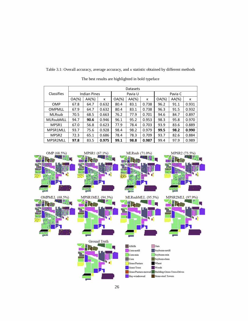
26
Table 3.1: Overall accuracy, average accuracy, and κ statistic obtained by different methods
The best results are highlighted in bold typeface
Classifies
Datasets
Indian Pines Pavia U Pavia C
OA(%) AA(%) κ OA(%) AA(%) κ OA(%) AA(%) κ
OMP 67.8 64.7 0.632 80.4 83.1 0.738 96.2 91.1 0.931
OMPMLL 67.9 64.7 0.632 80.4 83.1 0.738 96.3 91.5 0.932
MLRsub 70.5 68.5 0.663 76.2 77.9 0.701 94.6 84.7 0.897
MLRsubMLL 94.7 90.6 0.946 96.1 95.2 0.953 98.3 95.8 0.970
MPSR1 67.0 56.8 0.623 77.9 78.4 0.703 93.9 83.6 0.889
MPSR1MLL 93.7 75.6 0.928 98.4 98.2 0.979 99.5 98.2 0.990
MPSR2 72.3 65.1 0.686 78.4 78.3 0.709 93.7 82.6 0.884
MPSR2MLL 97.8 83.5 0.975 99.1 98.8 0.987 99.4 97.9 0.989

27
Figure 3.1: Classification maps obtained by different methods on AVIRIS Indian Pines dataset (overall
accuracy are reported in the parentheses).
3.3.3 Visual Comparison
Figure 3.1 shows the classification maps by different algorithms on the Indian Pines image. Generally
speaking, it indicates consistent results with the numerical measures. As we can see, algorithms
without MLL prior, i.e. OMP, MPSR1, MPSR2 and MLRsub produced intense artifacts in the
classification map due to the existence of mixed pixels in the image. Although all four algorithms
performed seemingly well, careful inspection indicates that MPSR2 yields fewer artifacts than the
others in certain classes, e.g. Grass/Pasture, Building-Grass-Tree-Drives and Soybeans-min. By
combining with MLL prior, MPSR1MLL, MPSR2MLL and MLRsubMLL produced very smooth
results, although there still exists misclassified patches in classes such as Soybeans-min and Building-
Grass-Tree-Drives. Nevertheless, some small classes such as oats were totally misclassified, because
of the lack of enough training samples for small classes. We also noticed that there are not much
difference between the map of OMPMLL and OMP.
3.3.4 Sensitivity of Parameters
The Section explored the sensitivity of two important parameters, i.e. sparsity level and smooth cost
for SR-based algorithms. Figure 3.2 plots the error bar of OA as a function of sparsity and smooth
cost based on the AVIRIS Indian Pines dataset.
Figure 3.2(a) indicates that MPSR-based algorithms achieved the highest performance when sparse
level was 3. And from sparsity level of 3, the performance of MPSR-based algorithms reduced quite
sharply. This is not surprising because increased sparsity level allows the wrong class to represent the
test sample equally well as the true class, consequently leads to the loss of discriminative power.
MPSR2MLL achieved higher OA than MPSR1MLL, and both MPSR1MLL and MPSR2MLL
outperform OMPMLL when sparsity level is lower than 30. OMP achieved stable results and
OMPMLL demonstrated slightly increased performance on high sparsity level.
In Figure 3.2(b), the increase in smooth cost increased the performance of MPSR1MLL and
MPSR2MLL to a stable level, but did not indicate noticeable influence on OMPMLL. Moreover,
MPSR2MLL achieved higher accuracy but lower variance than MPSR1MLL across most smooth-
cost levels, indicating the worth of accounting for the variance heterogeneity in MPSR.
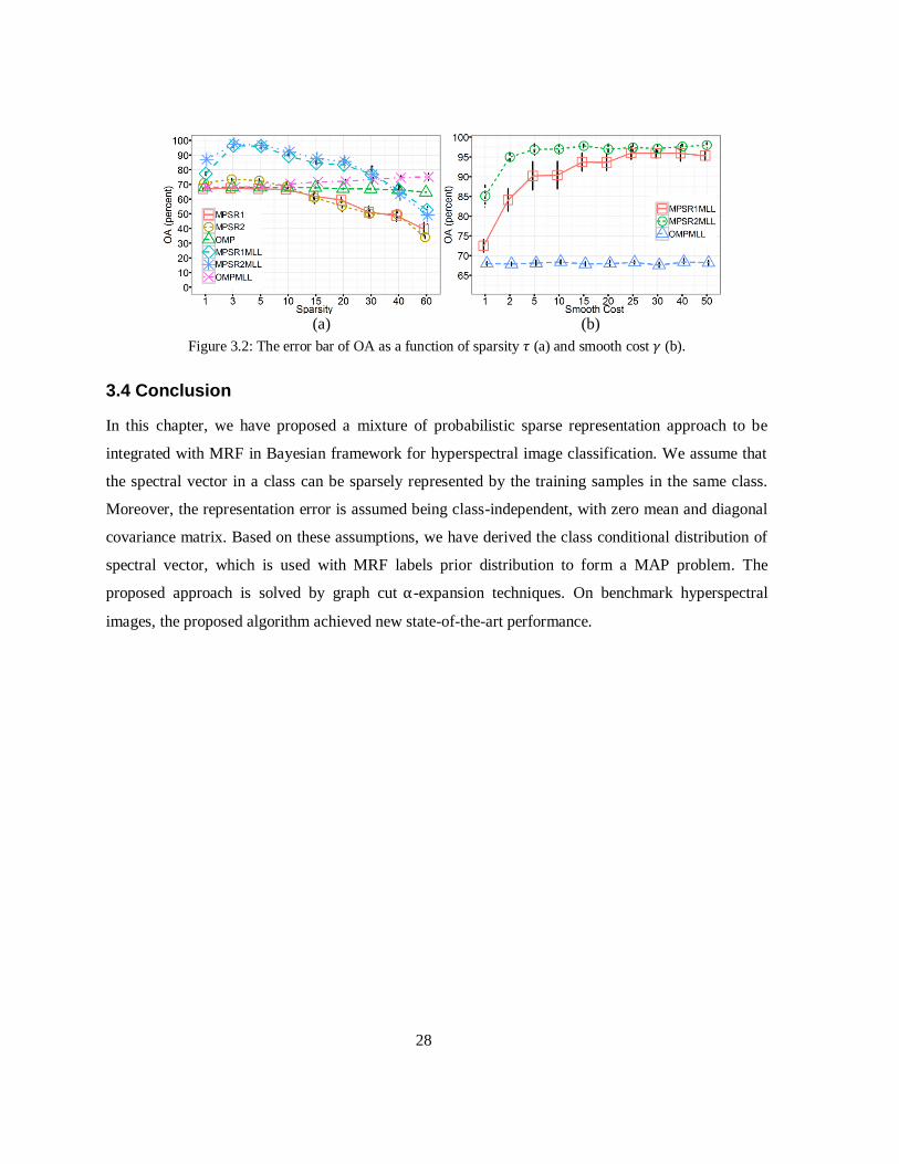
28
(a) (b)
Figure 3.2: The error bar of OA as a function of sparsity (a) and smooth cost (b).
3.4 Conclusion
In this chapter, we have proposed a mixture of probabilistic sparse representation approach to be
integrated with MRF in Bayesian framework for hyperspectral image classification. We assume that
the spectral vector in a class can be sparsely represented by the training samples in the same class.
Moreover, the representation error is assumed being class-independent, with zero mean and diagonal
covariance matrix. Based on these assumptions, we have derived the class conditional distribution of
spectral vector, which is used with MRF labels prior distribution to form a MAP problem. The
proposed approach is solved by graph cut -expansion techniques. On benchmark hyperspectral
images, the proposed algorithm achieved new state-of-the-art performance.

29
Chapter 4
K-P-Means for Spectral Endmember Estimation
This chapter presents K-P-Means, a novel approach for spectral endmember estimation. Spectral
unmixing is formulated as a clustering problem, with the goal of K-P-Means to obtain a set of
"purified" spectral pixels to estimate endmembers. The K-P-Means algorithm alternates iteratively
between two main steps (abundance estimation and endmember update) until convergence to yield
final endmember estimates. Experiments using both simulated and real spectral images show that the
proposed K-P-Means method provides strong endmember and abundance estimation results compared
to existing approaches. © [2014] IEEE. Reprinted, with permission, from [Xu Linlin, Li J., Wong, A.,
and Peng, J., K-P-Means: a clustering algorithm of K ―purified‖ means for spectral endmember
estimation, IEEE Geoscience and Remote Sensing Letters, 03/2014].
4.1 Introduction
Accurate estimation of the spectra of pure materials called endmembers is essential to spectral
unmixing that aims at estimating for each pixel the fractional abundances of endmembers. Current
methods for endmember estimation can be categorized as geometric, statistical and sparse coding
approaches (Bioucas et al., 2012). Although all these approaches have their own respective
advantages, it is undeniable that endmembers extraction would be more straightforward if we have
―pure‖ pixels that are due to individual endmembers, rather than multiple endmembers, for a number
of reasons. First of all, classical geometric approaches that rely on the presence of pure pixels, such as
vertex component analysis (VCA) (Nascimento & Bioucas-Dias, 2005) would achieve optimal
performance. More intuitively, if we know the group of pixels that are due to a particular endmember,
we can just use the mean value of pixels as an estimate of the endmember. Nevertheless, pure pixels
are rare to obtain directly from the hyperspectral images due to factors such as low spatial resolution
or the complexity of ground targets.
Given these considerations, this chapter therefore intends to explore the feasibility of obtaining
―purified‖ pixels from mixed pixels in order to achieve simplified yet efficient endmember estimation.
A ―purified‖ pixel is defined as the residual of mixed pixel after removing the contribution of all
endmembers except the one that dominates the pixel. We estimate ―purified‖ pixels in two steps
based on the abundance information of the hyperspectral image. First, we partition all pixels into
several groups that are dominated by different endmembers. Second, for pixels in each group, we
30
remove the contributions due to non-dominant endmembers in that group. In the first step, since a
cluster is defined by predominant endmembers, our approach differs from other label-utilizing
approaches (Zare & Gader, 2010; Castrodad et al. 2011; Martin & Plaza, 2011) in spectral unmixing
literature where a cluster may involve multiple significant endmembers. We treat the purified pixels
in each group as realizations of endmember subject to random noise, and thereby use the expected
value of the pixels as the endmember estimate. The resulting algorithm, which we will refer to as K-
P-Means algorithm alternates iteratively between two main steps (abundance estimation and
endmember update) until convergence to yield final endmember estimates. The capability of K-P-
Means is proved by experiments on both simulated and real hyperspectral images.
4.2 K-P-Means
4.2.1 Problem Formulation and Motivations
This chapter addresses a linear spectral unmixing model where the observed spectral pixels stack is
represented by endmember matrix and abundance matrix with independently identically
distributed (i.i.d.) Gaussian noise :
(4.1)
(
)
(
)
(
) (4.2)
where is a nonnegative abundance vector, that measures the contribution of endmembers
to dimensional spectral pixel :
∑ (4.3)
In most cases, the endmember collection contribute unequally to , and the group of pixels
dominated by is denoted by . Therefore, the image can be partitioned into K sets
. In order to reduce the coupling effect among endmembers, it is reasonable to infer
separately from pixels in . Nevertheless, mixed pixels in the same class may still
admit multiple endmembers. In order to further remove the influence of less-dominant endmembers,
it is desirable to use the proportion of that is solely due to the contribution of dominant endmember

31
to estimate , as opposed to using wholly. We refer to after removing the contribution of
less-dominant endmembers as ―purified‖ pixel.
Not only good abundance information can be utilized to obtain ―purified‖ pixels for enhanced
endmember estimation, but accurate endmember estimates can in turn boost the accuracy of
abundance estimation. Consequently, spectral unmixing can be treated as an iterative optimization
issue by taking advantage of the label information from the abundance. We therefore present in the
following Sections a K-P-Means clustering algorithm which intends to enhance endmember
estimation based on the ―purified‖ pixels by explicitly utilizing the label information.
4.2.2 K-P-Means Model
This Section formulates K-P-Means from a comparative perspective with the classical K-Means
algorithm. In K-Means, the spectral vector in class can be expressed as:
(4.4)
where is the mean vector of class and is class-independent white noise. Based on the
following objective function:
∑ ∑ ‖ ‖
(4.5)
where are the labels of pixels, K-Means algorithm iterates two steps:
estimating given , and estimating based on .
Similarly, the generative model of K-P-Means is formulated as:
∑
{ } (4.6)
where the general term in K-Means is expressed more specifically by ∑ . It means that
K-Means characterize a class by the mean vector , while K-P-Means defines the class by the
dominant endmember , whose abundance is the biggest. Therefore, comparing with K-Means
that considers the overall effect of a physical process, K-P-Means probes into the sources of the
physical process that contribute to the observations. The object function of K-P-Means can be
expressed as:
∑ ∑ ‖ ‖ (4.7)
where in objective function of K-Means is substituted by:
32
∑ . (4.8)
Therefore, as opposed to K-Means that adopts mixed pixels { } in class for estimating the mean
vector , K-P-Means excludes the contribution of less significant endmembers from estimating
dominant endmember . Accordingly, in the proposed algorithm can be treated as the mean
vector of ―purified‖ spectral pixels { }. That‘s why our algorithm is termed K-P-Means. Based on
above described model, K-P-Means iterates abundance estimation and endmember estimation, just as
the two steps in K-Means, which are introduced in Section 4.2.3 and 4.2.4 respectively.
4.2.3 Abundance Estimation
Following Eq. (4.7), given , pixel labeling requires solving the following optimization issue:
‖ ∑ ‖
s.t. { } { } (4.9)
It means that is associated with the th endmember which will take the largest coefficient
when representation error is minimized. Suppose are of similar scale, this optimization issue is
equivalent to firstly estimating by solving:
‖ ∑ ‖
s.t. (4.10)
then determining by:
(4.11)
As we can see, the estimation of abundance in Eq. (4.10) is essentially a non-negative least square
(NNLS) issue which can be efficiently solved by method in Lawson & Hanson (1974). Note that the
sum-to-one constraint is not necessary, since we only need the relative magnitudes of abundances to
determine dominant endmember. Therefore both K-Means and K-P-Means measure the ―relevance‖
of a pixel to different clusters in order to determine its label. Nevertheless for K-Means the ―relevance‖
is measured by the geometric ―closeness‖ from the pixel to class centers, while for K-P-Means, it is
measured by the magnitude of nonnegative contribution of endmembers to the representation of the
pixel in a least squares sense.
4.2.4 Endmember Estimation
Following Eq. (4.7), given , K-P-Means update based on the following generative model:

33
(4.12)
Since is i.i.d. zero-mean Gaussian noise, the maximum likelihood estimation (MLE) of is the
expected value of . Note that it is possible to apply other endmember extraction techniques, such
as VCA on to produces candidates of , it however will introduce extra problems, such as the
difficulty to determine the most relevant one.
4.2.5 Complete Algorithm
Assembling abundance estimation in Section 4.2.3 and endmember update in Section 4.2.4 into the
iterative optimization framework, leads to the complete algorithm of K-P-Means, which is detailed in
Algorithm 1. In endmember update step, in order to speed up convergence, the update of an
endmember is allowed to utilize the endmembers that have been updated. The iteration of the two
steps will stop if either the spectral angle difference (SAD, see Section 4.3) between endmember
estimates in two continuous iterations is smaller than a given value (i.e. ), or a predefined maximum
number of iteration (i.e. ) is reached.
Algorithm 1: K-P-Means
Input: spectral stack , number of clusters K and iteration threshold ;
Output: endmember and abundance ;
Initialization: ≔ , VCA ; or l l c l 𝑟
while or SAD do
(1) NNLS t , ← ;
(2) 𝐟𝐨𝐫
∑
( )
end for
end while
34
4.3 Experiments
4.3.1 Simulated Study
A 64×64 sized image with mixed pixels of 4 endmembers randomly selected from the USGS digital
spectral library (Clark et al., 1993) are simulated, following the procedure reported in Miao & Qi
(2007). Using the 4 endmembers, mixed pixels are created by firstly dividing the entire image into
8 8 sized homogeneous blocks of one of the 4 endmembers, then degrading the blocks by applying a
spatial low pass filter of 7 7. To further increase mixing degree, the remaining relatively ―pure‖
pixels with 80% or larger single abundance are forced to take equal abundances on all endmembers.
Zero-mean i.i.d. Gaussian noise is added to further degrade the image. The resulting image therefore
resembles a highly mixed hyperspectral image with measurement errors or sensor noise, which is very
challenging for spectral unmixing algorithms.
Two techniques, VCA [2] and MVC-NMF (Miao & Qi, 2007) are implemented using the code
provided by their authors. VCA represents classical techniques that rely on the existence of pure
pixels. Since VCA only extract endmembers, we estimate abundance using NNLS (Lawson &
Hanson, 1974). The comparison with MVC-NMF is desirable since both K-P-Means and MVC-NMF
deal with highly mixed pixels. MVC-NMF used as initial parameters the endmember estimated by
VCA, and 150 iterations in maximum.
Moreover, three variants of K-P-Means are implemented. K-P-Means used as initial parameters
both endmembers produced by VCA and pixels selected randomly from dataset, in order to explore
the sensitivity of K-P-Means to initial parameters. The resulting algorithms are referred to as K-P-
Means-VCA and K-P-Means-Random respectively. In K-P-Means-Random, 5 replicates are
performed, each with a new set of initial endmembers, to obtain the solution with smallest residual. In
order to prove the effectiveness of using ―purified‖ pixels in K-P-Means, we introduce for
comparison the ―non-purified‖ approach (i.e. K-nonP-Means), where instead of
is used in
Section 4.2.4 to update endmembers. All variants are implemented with =50 and =0.01 without
explicit explanation.
The consistency between estimated endmember and true endmember is measured by the widely
used spectral angle distance (SAD), defined as: SAD ‖ ‖‖ ‖ ⁄ , and the spectral
information divergence (SID), expressed as S D , where measures the
relative entropy between and (Chang & Heinz, 2000). The numerical measures for abundance

35
are achieved by replacing with in SAD and SID. The resulting measures are called AAD and AID
respectively.
The five methods are performed on simulated image to produce numerical measures. In order to
investigate the noise robustness of different methods, they are tested on images with different noise
levels measured by signal-to-noise ratio (SNR) (Miao & Qi, 2007). For each noise level, 20 images
with independent noise realizations are processed to obtain statistics of numerical measures, as
reported in Figure 4.1.
(a) (b)
(c) (d)
Figure 4.1: Performance comparison at different noise levels in terms of (a) SAD, (b) SID, (c) AAD and (b)
AID. In these four statistics, smaller value means better result.
Overall, K-P-Means-VCA achieved much smaller SAD and SID values than VCA, and close
results to MVC-NMF across all noise levels, indicating that K-P-Means is capable of extracting
accurately the endmembers in highly mixed and noisy circumstance. Moreover, the endmember
estimation of K-P-Means-VCA measured by SAD and SID seemed to be robust to noise level. As we
can see, SAD and SID remained at very low values with SNR decreasing from 45 to 20, although
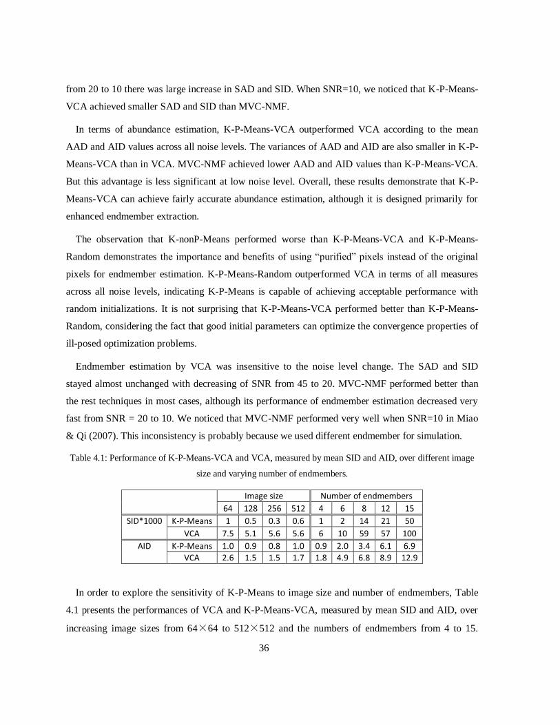
36
from 20 to 10 there was large increase in SAD and SID. When SNR=10, we noticed that K-P-Means-
VCA achieved smaller SAD and SID than MVC-NMF.
In terms of abundance estimation, K-P-Means-VCA outperformed VCA according to the mean
AAD and AID values across all noise levels. The variances of AAD and AID are also smaller in K-P-
Means-VCA than in VCA. MVC-NMF achieved lower AAD and AID values than K-P-Means-VCA.
But this advantage is less significant at low noise level. Overall, these results demonstrate that K-P-
Means-VCA can achieve fairly accurate abundance estimation, although it is designed primarily for
enhanced endmember extraction.
The observation that K-nonP-Means performed worse than K-P-Means-VCA and K-P-Means-
Random demonstrates the importance and benefits of using ―purified‖ pixels instead of the original
pixels for endmember estimation. K-P-Means-Random outperformed VCA in terms of all measures
across all noise levels, indicating K-P-Means is capable of achieving acceptable performance with
random initializations. It is not surprising that K-P-Means-VCA performed better than K-P-Means-
Random, considering the fact that good initial parameters can optimize the convergence properties of
ill-posed optimization problems.
Endmember estimation by VCA was insensitive to the noise level change. The SAD and SID
stayed almost unchanged with decreasing of SNR from 45 to 20. MVC-NMF performed better than
the rest techniques in most cases, although its performance of endmember estimation decreased very
fast from SNR = 20 to 10. We noticed that MVC-NMF performed very well when SNR=10 in Miao
& Qi (2007). This inconsistency is probably because we used different endmember for simulation.
Table 4.1: Performance of K-P-Means-VCA and VCA, measured by mean SID and AID, over different image
size and varying number of endmembers.
Image size Number of endmembers
64 128 256 512 4 6 8 12 15
SID*1000 K-P-Means 1 0.5 0.3 0.6 1 2 14 21 50
VCA 7.5 5.1 5.6 5.6 6 10 59 57 100
AID K-P-Means 1.0 0.9 0.8 1.0 0.9 2.0 3.4 6.1 6.9
VCA 2.6 1.5 1.5 1.7 1.8 4.9 6.8 8.9 12.9
In order to explore the sensitivity of K-P-Means to image size and number of endmembers, Table
4.1 presents the performances of VCA and K-P-Means-VCA, measured by mean SID and AID, over
increasing image sizes from 64×64 to 512×512 and the numbers of endmembers from 4 to 15.
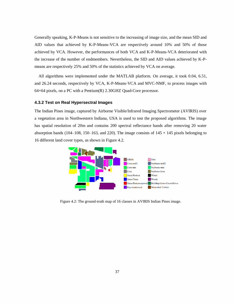
37
Generally speaking, K-P-Means is not sensitive to the increasing of image size, and the mean SID and
AID values that achieved by K-P-Means-VCA are respectively around 10% and 50% of those
achieved by VCA. However, the performances of both VCA and K-P-Means-VCA deteriorated with
the increase of the number of endmembers. Nevertheless, the SID and AID values achieved by K-P-
means are respectively 25% and 50% of the statistics achieved by VCA on average.
All algorithms were implemented under the MATLAB platform. On average, it took 0.04, 6.51,
and 26.24 seconds, respectively by VCA, K-P-Means-VCA and MVC-NMF, to process images with
64×64 pixels, on a PC with a Pentium(R) 2.30GHZ Quad-Core processor.
4.3.2 Test on Real Hypersectral Images
The Indian Pines image, captured by Airborne Visible/Infrared Imaging Spectrometer (AVIRIS) over
a vegetation area in Northwestern Indiana, USA is used to test the proposed algorithms. The image
has spatial resolution of 20m and contains 200 spectral reflectance bands after removing 20 water
absorption bands (104–108, 150–163, and 220). The image consists of 145 × 145 pixels belonging to
16 different land cover types, as shown in Figure 4.2.
Figure 4.2: The ground-truth map of 16 classes in AVIRIS Indian Pines image.

38
Figure 4.3: The abundance maps of eight selected endmembers extracted by K-P-Means-Random.
Figure 4.4: The abundance maps of the corresponding eight endmembers extracted by MVC-NMF.
In this experiment, K-P-Means-Random with =50 and =0.01 extracted a number of 20
endmemebers from pixels covered by ground truth classes. The abundance maps of eight selected
endmembers are shown in Figure 4.3. As we can see, the maps from left to right, top to bottom
correspond respectively to Grass/Trees, Hay-windrowed, Grass/Pasture, Soybeans-min, Corn-notill,
Wheat, Wood, and Stone-steel Towers. These correspondences between abundance maps and ground
truth classes may indicate that K-P-Means identified accurately the endmembers in the image,
considering that different endmembers tend to dominate different classes. Nevertheless, the bright
areas of most abundance maps do not match very well the ground truth, except Wheat and Stone-steel
Towers. It is not surprising considering the gap that while K-P-Means is designed to identify

39
individual endmembers, the pixels in the same ground truth class may actually assume multiple
significant endmembers, due to the complexity of ground targets in Indian Pines image.
Figure 4.4 shows the maps of the eight corresponding endmembers achieved by MVC-NMF, for
comparison purpose. As we can see, most endmember maps achieved by MVC-NMF do not match
the ground truth as well as the maps achieved by K-P-means, except the two maps correspond to
Wheat and Stone-steel Towers.
4.4 Conclusion
This chapter has presented a K-P-Means algorithm for spectral endmember extraction. Based on
abundance information, we proposed to obtain the ―purified‖ pixels from the original mixed pixels for
enhanced endmember estimation, which can in turn aid abundance estimation. Therefore, we
interpreted spectral unmixing as an iterative optimization problem, and designed the K-P-Means
algorithm which alternates iteratively between two main steps (abundance estimation and endmember
update) until convergence to yield final endmember estimates. Experiments on both simulated and
real hyperspectral images proved that K-P-Means is capable of estimating accurately both the
endmemebers and abundance.
40
Chapter 5
Clustering-based PCA for SAR Image Denoising
The combination of nonlocal grouping and transformed domain filtering has led to the state-of-the-art
denoising techniques. In this chapter, we extend this line of study to the denoising of Synthetic
Aperture Radar (SAR) images based on clustering the noisy image into disjoint local regions with
similar spatial structure and denoising each region by the Linear Minimum Mean-Square Error
(LMMSE) filtering in Principal Component Analysis (PCA) domain. Both clustering and denoising
are performed on image patches. For clustering, to reduce dimensionality and resist the influence of
noise, several leading principal components (PCs), identified by the Minimum Description Length
(MDL) criterion are used to feed the K-means clustering algorithm. For denoising, to avoid the
limitations of the homomorphic approach, we build our denoising scheme on additive signal-
dependent noise (ASDN) model and derive a PCA-based LMMSE denoising model for multiplicative
noise. Denoised patches of all clusters are finally used to reconstruct the noise-free image. The
experiments demonstrate that the proposed algorithm achieved better performance than the referenced
state-of-the-art methods in terms of both noise reduction and image details preservation. © [2014]
IEEE. Reprinted, with permission, from [Xu Linlin, Li J., Shu, Y., and Peng, J., SAR image denoising
via clustering-based principal component analysis, IEEE Transactions on Geoscience and Remote
Sensing, 03/2014].
5.1 Introduction
Synthetic Aperture Radar (SAR), as a coherent imaging system is inherently suffering from the
speckle noise, which has granular appearance and greatly impedes the automatic image processing
and visual interpretation. Although multilook averaging is a common way to suppress speckle noise at
the cost of reduced spatial resolution, it is more favorable to develop suitable filtering techniques.
Classical filters, such as Lee filter (Lee, 1980), Frost filter (Frost et al., 1982) and Kuan filter (Kuan et
al., 1985) that denoise SAR images in spatial domain by recalculating the center pixels of the filtering
windows based on the local scene heterogeneity, although work well in stationary image area, they
tend to either preserve speckle noise or erase weak scene signal at heterogeneous areas, e.g. texture
area, boundary, line or point targets. In order to better preserve image edges, Yu & Acton (2002)
designed a speckle reduction anisotropic diffusion (SRAD) method which can be treated as an edge-
sensitive version of the classical filters. The performance of the Gamma MAP filter (Lopes et al.,
41
1990), which denoises SAR image via maximum a posteriori criteria, depends highly on whether the
imposed Gamma distribution can accurately describe SAR image.
Instead of denoising in spatial domain, it has been proved more efficient to perform the task in
transformed domain where signal and noise are easier to separate. The wavelet techniques assume
that noise mainly exists on the high frequency wavelet components and thus can be removed by
filtering the wavelet coefficients in transformed domain. This idea has proved great success to
denoise additive white Gaussian noise (AWGN). To adapt wavelet for SAR denoising, many
techniques adopted the homomorphic approach where speckle noise subject to log-transformation is
treated as AWGN and denoised in wavelet domain by thresholding (Gagnon & Jouan, 1997; Guo et
al., 1994) or modeling (Achim et al., 2003; Solbø & Eltoft, 2004; Bhuiyan et al., 2007) the wavelet
coefficients. However, since the performance of denoising is very sensitive to logarithmic operation
that tends to distort the radiometric properties of SAR image, techniques based on additive signal-
dependent noise (ASDN) model were developed in (Argenti & Alparone, 2002; Xie et al., 2003;
Argenti et al., 2006; Argenti et al., 2008).
Although wavelet-based denoising methods have proved better efficiency than classical filters,
limitations reside in the inadequate representation of various local spatial structures in images using
the fixed wavelet bases (Muresan & Park, 2003; Zhang et al., 2010; He et al., 2011). On the other
hand, locally learnt Principal Component Analysis (PCA) bases, a series of mutually orthogonal
directions with sequentially largest variances, have shown better capability of representing structural
features, e.g. image edges and texture. In PCA domain, the scene signal is mostly captured by several
leading Principal Components (PCs), while the last few components with low variances are mainly
due to noise. The denoising of AWGN has been achieved by filtering the PCs through linear
minimum mean-square error (LMMSE). Examples include the adaptive PCA denoising scheme
proposed by Muresan and Parks (2003) and local pixel grouping PCA (LPG-PCA) algorithm
proposed by Zhang et al. (2010). Both methods have proved to be more effective than the
conventional wavelet-based denoising methods. However, no efforts have been made to adapt PCA-
based denoising to SAR images. Since SAR images assume signal-dependent noise, a new denoising
model that takes into account this particularity is required.
A different line of research initiated in Buades et al. (2005) approaches image denoising as a
nonlocal means (NLM) problem, where ‗nonlocal‘ pixels whose neighborhoods share similar spatial
structure, rather than ‗local‘ pixels that are just geometrically near to each other are used to perform
42
weighted average with the weights measured by the Euclidean distances between the referenced
image patch and the other candidate patches. The NLM method has been adapted for SAR image
denoising by adjusting the similarity measure to the multiplicative nature of speckle noise (Coup et al.,
2008; Zhong et al., 2009; Deledalle et al., 2009). Particularly, the probabilistic patch-based (PPB)
algorithm in Deledalle et al. (2009) proved to achieve the state-of-the-art performance for SAR image
denoising. Moreover, the idea of NLM has been extended to combine with the transformed domain
denoising approaches, leading to the state-of-the-art image denoising techniques, e.g. the block-
matching 3D filtering (BM3D) (Dabov et al., 2007), LPG-PCA (Zhang et al., 2010) and SAR-BM3D
(Parrilli et al., 2012) algorithms. All methods take advantage of the enhanced sparsity in transformed
domain when denoising is performed on image patches with similar structure. In these methods,
block-matching approach was adopted to find for each patch in the image a group of similar patches.
However, this approach faces the difficulty to define the threshold as to how ―similar‖ to the
reference patch is acceptable. It also has high computational cost.
In this study, we extend this line of study to denoise SAR images by explicitly addressing two
issues. First, we build a new denoising model based on PCA technique to account for the
multiplicative nature of speckle noise. Based on ASDN model, we derive a LMMSE approach for
solving PCA-based denoising problem. Our approach is the first to build the PCA-based denoising
method on the ASDN model for SAR image denoising. Besides SAR images, it is also applicable to
other signal-dependent noise. Second, instead of using block-matching approach, we employ a
clustering approach. We propose to use the combination of log-transformation, PCA and K-means
methods for finding similar patches. Based on the statistical property of speckle noise, we proved the
compatibility between PCA features and the K-means model. This clustering approach proved to be
an competitive alternative to the block-matching approach adopted in Zhang et al. (2010), Deledalle
et al. (2009) and Parrilli et al. (2012).
The rest of the chapter is organized as follows. Section 5.2 discusses data formation and PCA
analysis. Section 5.3 derives the LMMSE filtering of speckle noise in PCA domain. Section 5.4
details the clustering-based scheme for SAR image denoising. In Section 5.5, the complete procedure
of the proposed strategy that involves a second stage is discussed. In Section 5.6, experiments are
designed to compare the proposed method with other popular denoising techniques. Results obtained
using both simulated and real SAR images are presented and discussed. Section 5.7 concludes this
study.

43
5.2 Data Formation & PCA Analysis
The SAR image as a collection of all the image patches is represented by a data matrix
(5.1)
where denotes the number of pixels, and ( ) is a vector, representing the th
patch which is a small square window centered at the th pixel.
Figure 5.1: Illustration of the acquisition of a patch in SAR image.
The PCA can be achieved by performing Singular Value Decomposition (SVD) on the covariance
matrix of :
(
)
(
)
(
)
(
)
(5.2)
where element in represents the covariance between the two pixels at position and
across the image. So provides a statistical description of the relationship among pixels in SAR
image. Pixels that do not belong to the same patch are considered uncorrelated. Thus the size of the
patch determines the scale of spatial patterns that can be captured. Generally speaking, bigger sized
patch considers larger range correlations and hence is more capable of capturing larger-scale repeated
patterns in SAR image. , vectors, denote the sequence of mutually orthogonal
PCA bases onto which the projection of patches stack produces the PCs with sequentially largest
variances represented by .
In PCA domain, several leading PCs capture most of the scene signal in image patches, while the
last few components are mostly due to noise. In this chapter, we use PCA for both denoising and
feature extraction. In Section 5.3, we develop a LMMSE criterion based on ASDN model to shrink
the PCs. Thus denoising can be achieved by reconstructing SAR image using the processed PCs. In
SAR image
Patch variable
44
Section 5.4, we use several leading PCs in logarithmic space identified by the Minimum Description
Length (MDL) criterion to feed the K-means algorithm. This not only reduces the dimensionality and
de-correlates the spatial variables, but also suppresses the noise contained in image patches.
5.3 SAR Image Denoising in PCA Domain
In Muresan & Parks (2003) and Zhang et al. (2010), the LMMSE shrinkage was conducted in PCA
domain to remove AGWN. For SAR speckle noise, we can certainly adopt the homomorphic
approach and apply the same methods in Muresan & Parks (2003) and Zhang et al. (2010). However
since the performance of denoising is sensitive to log-transformation that tends to distort the
radiometric dynamics of the SAR data, it is more appropriate to perform denoising in original space
instead of logarithmic space. In this Section, we derive a new LMMSE shrinkage approach under the
ASDN model. We assume the speckle noise is fully developed, thus a SAR image pixel can be
modeled as:
(5.3)
where , , and represent respectively unobserved scene signal, speckle noise and the observed
signal. Based on Eq. (5.3), we get the ASDN model as:
(5.4)
where . Because has unit mean, thus is a zero-mean signal-dependent noise.
Hence the patch variable in SAR image can be described by.
(5.5)
where ,
, . Denote the covariance
between and by
, and the mean of by , we can get:
(5.6)
For fully developed speckle noise, and are uncorrelated, so we get . Because
, we get . So
45
( ) (5.7)
We assume speckle noise is spatially uncorrelated, i.e. for . Thus we have:
(5.8)
In the following analysis, we represent the empirical mean of the patches in by and we assume
that the patch variable has been centralized. Denote the covariance of by , the PCA bases can
be obtained by performing SVD on :
(5.9)
where the column vectors in represent the PCA bases with sequentially largest variances, is the
diagonal matrix of the variances of PCs, which are the projection of patch variables onto PCA bases:
(5.10)
where and stand respectively for the signal and noise parts in the projection.
If is known, denoising can be achieved by performing inverse PCA transformation using . In
this research, is estimated by LMMSE criterion.
( ) ( )
(5.11)
The th element of can be estimated through the following equation:
( )
{∑
∑
} ∑
∑
{∑∑
} ∑∑
46
∑∑ [
]
∑∑
∑
∑ ∑
(5.12)
Denote . Because and are uncorrelated for fully developed speckle noise, we can
get
( ) *( )
+ (
)
= ( ) (5.13)
From Eq. (5.13) and Eq. (5.7), we get
(
), so
∑ *
(
)+ ∑ ∑
(5.14)
From Eq. (5.8), we get
for , so
∑ *
(
)+ ∑ ∑
(5.15)
In Eq. (5.15), can be calculated from the theoretical distribution of speckle noise, e.g. for
Gamma distribution (Xie et al., 2002), where L stands for the ENL. is the
element of in Eq. (5.9). ( ) and
are estimated by the respective empirical values: ( )
, , where stands for the element of and stands
for the element of .
Given in Eq. (5.11), the noise-free image patch can be obtained by performing inverse PCA
transformation:
(5.16)
The denoised patches will finally be used to construct the noise-free SAR image.
5.4 Clustering Scheme
The effectiveness of denoising in PCA domain depends highly on whether the PCs can sparsely
represent the scene signal. And the sparsity can be achieved by performing analysis on patches with
similar spatial structure. There are two approaches for finding similar patches, block-matching and

47
clustering. Block-matching is a supervised approach, which finds, for each pixel on the image, a
group of patches that are ―similar‖ to the reference patch. This approach has high computational cost.
Since it is hard to define the ―threshold‖ as to how ―similar‖ to the reference patch is acceptable, the
researchers always turn to guarantee a minimum number of similar patches. However, it may render
some of the selected patches less relevant to the referenced patch. As opposed to the block-matching
approach adopted in BM3D and NLM, the clustering approach involved in the proposed approach
finds similar patches in an unsupervised manner by adaptively partitioning the image into disjoint
areas. It requires less computation. Moreover, since the ―threshold‖ in clustering approach is
adaptively determined by comparing the proximities of the candidate patch to different cluster centers,
rather than being pre-defined, the clustering approach is supposed to be more capable of finding
relevant patches than block-matching approach.
In this study, we adopt K-means algorithm (Lloyd, 1982) proposed by Lloyd considering its
simplicity and speed. And we use the Euclidean distance to measure similarity in feature space.
Performing K-means clustering on image patches also faces problems, such as high dimensionality,
high correlation among features, and intense iterations due to poor initial parameter values. In this
study, we adopt log-transformation and PCA to extract compact features to feed the K-means
algorithm.
This Section is organized as follows: we start with the illustration of feature extraction techniques;
we then prove the compatibility of the extracted features and K-means algorithm; lastly, we discuss
parameter tuning and efficient realizations of the clustering algorithm.
5.4.1 Feature Extraction
Before extracting features for clustering, we apply log-transformation on original SAR image as a
pre-processing step. It has been common practice to aid clustering by preprocessing heavy tail
distributed variables using log-transformation (Liu et al., 2003; Liu et al., 2007). In particular, Liu in
Liu et al. (2003) indicated that log-transformation significantly improved the clustering result, and Liu
et al. (2007) demonstrated a 10% increase in clustering accuracy after applying the log-transformation.
The speckle noise in SAR image follows Gamma distribution that is long-tailed. Moreover, speckle
noise is signal-dependent which means it has bigger variance on brighter image areas. This unstable
nature would produce large between-cluster overlapping. So the log-transformation is used here to de-
skew the dataset and to stabilize the variance. The log-transformed data tends to be symmetrically
48
distributed with constant variance, thus is more desirable for statistical methods, such as PCA and K-
means algorithms.
Although clustering can be performed directly on image patches, it always suffers from high
dimensionality e.g. 5 5 patch produces 25 variables, and the intense speckle noise contained in the
patch. In order to solve these problems, we adopt PCA as a feature extraction technique. Only
leading PCs that are mostly due to signal are used as features for clustering. The accurate estimation
of is important in the sense that the underestimation would lose useful information but
overestimation would introduce noise and unnecessary computation cost. One popular approach
determines by setting a threshold to the percentage of variation explained by signal components.
This approach is simple but rather subjective. In this study, we estimate by MDL criterion which
was proposed by Rissanen (1978) and has been used to determine the number of signals in Wax &
Kailath (1985). The dimensional image patch variable subject to log-transformation can be
represented by the following equation:
∑ (5.17)
where is the eigenvector matrix, whose ith column denotes the th PCA bases, and
denotes the log-transformed speckle noise that roughly satisfies Gaussian distribution with zero mean
and diagonal covariance matrix . We assume that the scene signal can be reconstructed by the
first K PCs
∑ (5.18)
where stands for the th PC. We can see that Eq. (5.17) is same with Eq. (1) in Wax
and Kailath (1985), where the authors estimated the number of signals by
∑
∏
(5.19)
where stands for the th biggest eigenvalue of , denotes the number of observations.
can be easily determined by comparing all the solutions.
5.4.2 The Compatibility of PCA Features and K-means algorithm
K-means algorithm that relies on Euclidean distance implicitly assumes that the noise of input
features satisfies independent and identically Gaussian distribution. In the following, we prove that
PCA features described above satisfies this assumption. We reformulated Eq. (5.17) as:
49
(5.20)
Since and are independent for fully developed speckle noise, we can get:
(5.21)
where and denotes respectively the covariance matrix of and . The PCA analysis can be
achieved by performing SVD on .
(5.22)
where the column vectors in represent the PCA bases, is eigenvalue matrix.
Then, we have:
[
] (5.23)
So we can see that and share the same PCA bases. As in Eq. (5.10), the PCA features can be
obtained by projecting image patch onto PCA bases:
(5.24)
where and stand respectively for the signal and noise parts in PCA feature.
Denote the variance matrix of by :
[
] [
] (5.25)
Since , the assumption of K-means algorithm on noise distribution can be well satisfied.
Although this property could not guarantee the convergence of K-means algorithm to global
minimum, it provides theoretical assurance that K-means performance can be optimized.
5.4.3 Parameters tuning and efficient realization
Number of clusters: The number of clusters in the image depends on the definition of what
constitutes a cluster. This issue is mostly application-oriented, e.g. for background subtraction,
background and foreground should be represented as two clusters, but in content-based image
analysis, the number of cluster is mainly determined by the number of objects in the image. Here we

50
have no high-level requirements on the notion of cluster, but only loosely constraint that a cluster is a
collection of image patches with similar spatial structure. Thus the number of clusters cannot be and
does not need to be estimated very accurate. A loose cluster can be splitted into several compact ones,
which does not have too much influence on the denoising results. Nevertheless, the rough estimation
of the number of patterns exist in the image is still important because overly underestimation would
reduce the sparsity in PCA domain and the opposite would increase computation burden and also
preserve unnecessary artifact. So the number of cluster can be better determined based on the
complexity of scene. More complex image should be assigned more clusters to fully capture image
details. Since PCA detects statistically uncorrelated sources, a more complex image scene tends to
have larger number of signal PCs. So we use the number of signal PCs in Section 5.4.1 as
estimate of the number of clusters. Moreover, to prevent over-segmentation, we set an upper limit on
. In this study, we require:
(5.26)
Size of cluster: The number of patches in each cluster should be big enough for efficient
estimation of the covariance matrix . In this study, we constrain that each cluster should have at
least 50 members. A cluster smaller than this value will be deleted and its members will be dispersed
into the other clusters based on the proximity in Euclidean space.
Initial cluster centers: K-means clustering is very sensitive to initial parameter values. Poor
assignment of initial parameters may cause longer time to converge. Because the PCs provide a
contiguous membership indicator for K-means clustering (Ding & He, 2004), we estimate the labels
of image pixels by sorting the values of the first PC and then splitting them evenly into groups.
Given the initial labels, we estimate the centroids for each group.
Deal with large image: SAR images always have big size. Clustering on them directly tends to
ignore weak patterns that involve small number of pixels. Hence some image details would be erased
during the denoising stage. So in this study, a large image is divided into several sub-images which
are denoised separately. The final noise-free image is reconstructed by all the denoised sub-images.
There are no universal standard for the size of the sub-image. It should be adjusted according to the
complexity of the image scene. Small size should be preferred for image with complex scene. For
SAR image, a size of 64 64 pixels can achieve a good result based on our experiments. To avoid the
boundary artifacts between neighboring sub-images, we design the neighboring sub-images to be
51
slightly overlapping. Based on our experiment, an overlapping of 5 pixels would produce smooth
boundaries.
Size of patch: As discussed in Section 5.3, patch with big size can capture large scale patterns but
would also increase the computation cost. For SAR images that are without strong texture patterns,
the size of 3 3 pixel is sufficient according to our experiments. But larger patch size, such as 5 5 is
required for heavily textured images.
5.5 Complete Procedure of the Proposed Approach
The complete procedure involves two stages (Figure 5.2): the first stage produces a denoised image
which is referenced as a clean image in the second stage to feed the clustering algorithm and to aid
the LMMSE shrinkage. The detailed procedure is given below:
Stage 1: The original SAR image is split into N sub-images which are M M sized (M=64). For
each sub-image, we repeat the steps of clustering and denoising, until all sub-images have been
processed. Finally, we aggregate the denoised patches to produce the denoised SAR image.
Clustering: This step intends to identify image pixels whose neighborhoods have similar spatial
structure. The ith sub-image is firstly log-transformed. Then we extract all the S S sized patches (S=5)
to form a data matrix which is then transformed into the PCA domain. The first PCs are used to
feed the K-means algorithm, where is given in Section 5.4.1. The number of cluster is
determined by Eq. (5.26). Other parameters, i.e. the size of cluster and the initial cluster centers are
given in Section 5.4.3. The products of this step are the labels of all pixels in the ith sub-image.
Denoising: Given the labels, this step aims to denoise the ith sub-image. Image patches in each
cluster are denoised separately. Note that the image patches are extracted from the original SAR
image. For each cluster, patches of pixels belong to this cluster are extracted to form a data matrix.
We calculate the empirical mean and variance matrix . Then the patches are denoised by the
following operations: obtaining PCA bases (Eq. (5.9)), projecting onto PCA bases (Eq. (5.10)),
shrinking PCs in PCA domain (Eq. (5.11), (5.15)), and transforming back into patch domain (Eq.
(5.16)). This step does not stop until all the clusters in the ith sub-image have been denoised. The
final product of this step is a collection of denoised patches in the ith sub-image.
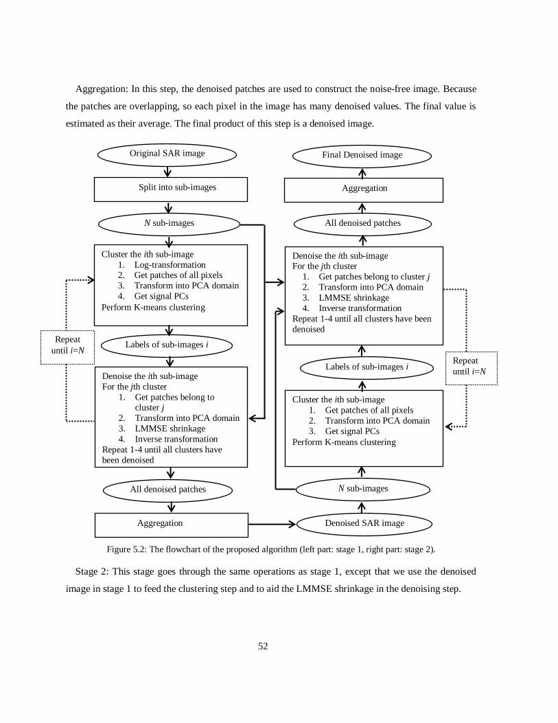
52
Aggregation: In this step, the denoised patches are used to construct the noise-free image. Because
the patches are overlapping, so each pixel in the image has many denoised values. The final value is
estimated as their average. The final product of this step is a denoised image.
Figure 5.2: The flowchart of the proposed algorithm (left part: stage 1, right part: stage 2).
Stage 2: This stage goes through the same operations as stage 1, except that we use the denoised
image in stage 1 to feed the clustering step and to aid the LMMSE shrinkage in the denoising step.
Original SAR image
Split into sub-images
N sub-images
Cluster the ith sub-image
1. Log-transformation 2. Get patches of all pixels
3. Transform into PCA domain
4. Get signal PCs
Perform K-means clustering
Labels of sub-images i
Denoise the ith sub-image
For the jth cluster
1. Get patches belong to cluster j
2. Transform into PCA domain
3. LMMSE shrinkage
4. Inverse transformation
Repeat 1-4 until all clusters have
been denoised
All denoised patches
Aggregation Denoised SAR image
Repeat
until i=N
N sub-images
Cluster the ith sub-image
1. Get patches of all pixels
2. Transform into PCA domain
3. Get signal PCs
Perform K-means clustering
Labels of sub-images i
Denoise the ith sub-image For the jth cluster
1. Get patches belong to cluster j
2. Transform into PCA domain
3. LMMSE shrinkage
4. Inverse transformation
Repeat 1-4 until all clusters have been
denoised
All denoised patches
Aggregation
Repeat
until i=N
Final Denoised image

53
Clustering: Instead of the original SAR image, the denoised image produced in stage 1 is used for
clustering to get the labels. Moreover, the log-transformation is avoided. Other operations are the
same with stage 1.
Denoising: The denoising procedures on this stage are the same with stage 1, except that we use the
denoised image in stage 1 to estimate in Eq. (5.11). Given labels, we extract two set of patches for
each cluster. One set is from the original SAR image. This set is to be denoised. Another set is from
the denoised image produced by stage 1. This set is treated as a collection of signal patches. Hence
the covariance matrix of signal patches can be estimated as the sample covariance matrix. The
shrinkage of the first set of patches in PCA domain requires the estimation of . Here, instead of
using Eq. (5.15), we use:
(27)
Aggregation: The denoised patches are used to estimate the final noise-free image. The aggregation
procedures are the same with stage 1.
Stage 2 is basically a repetition of stage 1, except that we used the denoised image in stage 1 to
perform clustering and to estimate in Eq. (5.11). These modifications are motivated by the fact
that the first stage can significantly suppress SAR speckle noise and achieve a cleaner image. Hence
using the denoised image, instead of the noisy image can achieve more accurate clustering results.
Moreover, treating the denoised image as clean image to estimate is more efficient than
performing shrinking on the noisy image. A second stage in the BM3D algorithm (Dabov et al., 2007)
was motivated by similar considerations.
5.6 Results and Discussion
In this study, both simulated and real SAR images are used to test the proposed SAR denoising
method. In order to achieve a quantitative evaluation, clean images are degraded by adding
multiplicative noise. Thus we can treat the clean image as the true values and use numerical measures
to evaluate the performance. Although the true values of real SAR images are unknown, we can
achieve qualitative assessments based on visual interpretation. In this experiment, three other methods
(i.e. PPB (Deledalle et al., 2009), LPG-PCA (Zhang et al., 2010) and SAR-BM3D algorithm (Parrilli
et al., 2012)) are selected to compare with the proposed method. The selection of these methods is
based on the considerations of both the availability of the codes and their relevance to our work. The
54
LPG-PCA represents the state-of-the-art denoising techniques for images with additive noise, while
PPB and SAR-BM3D are the state-of-the-art methods for SAR image. Because LPG-PCA was
designed to deal with additive noise, to adapt it to SAR image, we transform the speckle noise into
additive noise by logarithmic operation before performing it on noisy SAR images. The biased means
caused by log-transformation are also corrected. In all experiments, without explicit indication, the
parameters of the above algorithms are set as suggested in the referenced papers, and our method is
implemented by setting the patch size to be 5 5 pixels and the sub-images to be 64 64 pixels with 5
pixels overlapping with their neighbors. All the other parameters in our method are determined by the
methods in Section 5.4.3.
5.6.1 Test with Simulated Images
A variety of image sources are considered in this experiment, including the benchmark test image, i.e.
the Barbara (Figure 5.3a) in the image denoising literature, and the high-resolution optical satellite
(i.e. IKONOS) image whose scene structure is similar to real SAR image (Figure 5.3b). An ideal SAR
denoising method is required to be capable of removing speckle effectively, while in the meantime
preserving image details (e.g. texture, edge and line target) that constitute the desired features for
further analysis. So in order to fully examine the abilities of details preservation, an image comprising
two texture parts with a smooth boundary is designed to be used in this experiment. As shown in
Figure 5.3(c), the left part of the image is weakly textured with a wave-like appearance while the right
part is with a strong mesh texture. Thus the performance of denoising methods on image with
changing scene complexities can be investigated. Simulated SAR image are obtained by multiplying
speckle noise with these clean images. In this experiment, we use speckle noise in amplitude format
which satisfies a squared-root Gamma distribution (Xie et al., 2002). All images are degraded with
four different levels of speckle noise, i.e. the ENL (denoted by L) equals to 1, 2, 4 and 16,
respectively. To avoid randomness, 20 noisy images for each clean image are produced by
multiplying different noise realizations. All noisy images are processed and the numerical evaluation
is based on the average of the results.
In this study, two statistics (i.e. Signal-to-Mean-Square-Error Ratio (S/MSE) and ) are used to
evaluate these denoising methods. S/MSE corresponding to SNR in case of additive noise is a very
effective measure of noise suppression in multiplicative case (Gagnon & Jouan, 1997). On the other
hand, to measure image detail preservation we employ originally defined in Sattar & Floreby
(1997). should be equal to unity for an ideal detail preservation.

55
The zoom of denoised images by different methods when are shown in Figure 5.4-5.6, and
the values of the two statistics for , 2, 4 and 16 are summarized in Table 5.1, in which the best
value in each unit is bold. Overall, it shows in Table 5.1 that the proposed method outperformed the
other referenced algorithms in terms of both measures. This demonstrates that our method is good
both at speckle noise suppression and image detail preservation. The row ‗prop.stage1‘ in Table 5.1
was achieved by the first stage of our method. Comparing with row ‗prop.‘, we can see that the
second stage involved in our method can significantly improve the results. The row ‗prop.global‘ in
Table 5.1 was achieved by performing PCA denoising on the sub-images without the clustering step.
The observation that values in ‗prop.global‘ are lower than values in ‗prop.‘ justifies the clustering
approach in the proposed method.
Both LPG-PCA and the proposed method denoise SAR images in PCA domain. However, LPG-
PCA works on AWGN obtained by performing log-transformation on SAR image, while the
proposed method takes into account the multiplicative nature of speckle noise by building the
denoising approach on ASDN model. The observation that the proposed method greatly outperformed
LPG-PCA on most noise levels justifies the proposed denoising model for ASDN. We also observed
that the performance of LPG-PCA is very sensitive to noise levels variation in logarithmic space. As
we can see in Table 5.1, when L=1, LPG-PCA achieved lower statistics than the proposed method.
But with the increasing of L, LPG-PCA tends to achieve comparable results with our method in terms
of β. LPG-PCA even achieved higher β on image Barbara when and 16. This is reasonable
because LPG-PCA was designed for AWGN. When L is big, the speckle noise subject to logarithmic
operation is very close to Gaussian white noise. Therefore, the method can achieve good results.
However, when L is small, speckle noise begins to deviate from Gaussian distribution and its mean
value is no more zero. This discrepancy between empirical data and the model assumption may
reduce the efficiency of LPG-PCA. As we can see, the images in Figs. 5.4-5.6 denoised by LPG-PCA
show many small artifacts, while images by the proposed method have little artifacts but plenty image
details.
It is noticed that our method was especially better at denoising the synthesized texture image
(Figure 5.3c). In Figure 5.6, the image produced by the proposed method is the most similar to clean
image. The images denoised by PPB and SAR-BM3D are blurred and the holes in boundary area are
erased. The image produced by LPG-PCA has clear textural patterns, but assumes many artifacts. The
statistics in Table 5.1 indicates consistent results. The proposed method achieved high values in both

56
measures, indicating good performance on both noise removal and detail preservation. In contrast,
LPG-PCA achieved small S/MSE values, while PPB and SAR-BM3D achieved small values. The
clustering approach involved in the proposed method may have contributed to the superiority of the
proposed method in dealing with textual images. In texture image, the increased scene complexity
renders it difficult to find similar patches. Given the difficulty, the clustering approach might find
more relevant patches than block-matching approach, leading to better preservation of texture patterns.
On less-textured image, i.e. IKONOS, the proposed approach also achieved higher values, and
preserved more image details than the other methods. The observation that LPG-PCA and the
proposed method outperformed SAR-BM3D in terms of detail preservation in highly textured image
(i.e. Figure 5.6) may suggest that the PCA-based denoising approach is more efficient at dealing
textural structures.
A good denosing method should be capable of removing speckle noise without sacrificing image
details. PPB tended to erase image details too much. In Figs. 5.4-5.6, we see that the denoised images
by PPB have very smooth appearances but also blurred boundaries and reduced details information.
On the IKONOS image, LPG-PCA achieved higher S/MSE but lower values than SAR-BM3D,
while on the Syntexture image, LPG-PCA achieved lower S/MSE but higher values. Our method
achieved very high S/MSE and values on most images.
The SAR-BM3D and PPB algorithms were implemented using the C language, while the other
algorithms were implemented under the MATLAB platform. All the computations were conducted on
a PC with a Pentium(R) 2.30GHZ Quad-Core processor. On average, it took 36.8, 53.1, 34.7 and 23.5
seconds, respectively by PPB, LPG-PCA, SAR-BM3D and the proposed method to process a
256×256 pixels simulated image. It is fair to compare the time efficiency of the proposed algorithm
and LPG-PCA, because both methods are PCA-based and implemented in MATLAB language. The
observation that the proposed algorithm consumes less than half of the time of LPG-PCA
demonstrates the efficiency of clustering algorithm than block-matching approach. This conclusion is
also supported by the shorter processing time of our algorithm than PPB and SAR-BM3D, especially
considering the fact that C language is more efficient than MATLAB.

57
(a) (b) (c)
Figure 5.3: Clean images used in this study, (a) Barbara, (b) Optical satellite image (IKONOS), (c) Synthesized
texture image. All images are 256×256 pixels big.
Table 5.1: Results (s/mse and ) on three images with different noise levels
IKONOS Barbara Syntexture
L=1 L=2 L=4 L=16 L=1 L=2 L=4 L=16 L=1 L=2 L=4 L=16
S/MSE
noisy PPB
LPG-PCA SAR-BM3D
Prop. Prop.stage1 Prop.global
6.68 14.99 16.70 14.85 17.17 13.89 12.25
9.35 16.56 18.06 15.04 18.10 15.90 14.04
12.19 17.97 19.43 18.04 19.70 18.67 15.63
18.10 21.26 21.15 21.97 22.24 22.87 20.05
6.69 16.27 16.84 16.93 17.29 14.83 12.98
9.35 17.08 17.11 17.19 18.27 16.64 14.67
12.18 18.76 18.49 17.31 18.75 17.38 15.71
18.11 19.20 19.41 19.58 19.80 19.46 18.39
6.69 11.41 10.73 15.89 18.95 13.31 10.65
9.35 11.10 12.45 17.29 20.30 15.73 13.06
12.18 11.95 14.74 16.55 21.28 17.59 14.65
18.09 17.76 19.99 18.60 23.99 21.75 18.71
β
noisy PPB
LPG-PCA SAR-BM3D
Prop. Prop.stage1 Prop.global
0.183 0.323 0.364 0.484 0.495 0.376 0.321
0.246 0.470 0.527 0.576 0.598 0.498 0.401
0.333 0.567 0.658 0.658 0.685 0.616 0.491
0.572 0.696 0.796 0.804 0.829 0.804 0.687
0.167 0.519 0.616 0.708 0.719 0.562 0.472
0.223 0.663 0.738 0.771 0.788 0.668 0.576
0.304 0.765 0.852 0.835 0.845 0.760 0.675
0.534 0.873 0.917 0.897 0.913 0.883 0.826
0.252 0.599 0.730 0.663 0.792 0.655 0.522
0.335 0.640 0.791 0.729 0.835 0.751 0.596
0.441 0.697 0.838 0.783 0.868 0.815 0.671
0.695 0.818 0.893 0.783 0.920 0.899 0.812
(a) (b) (c)
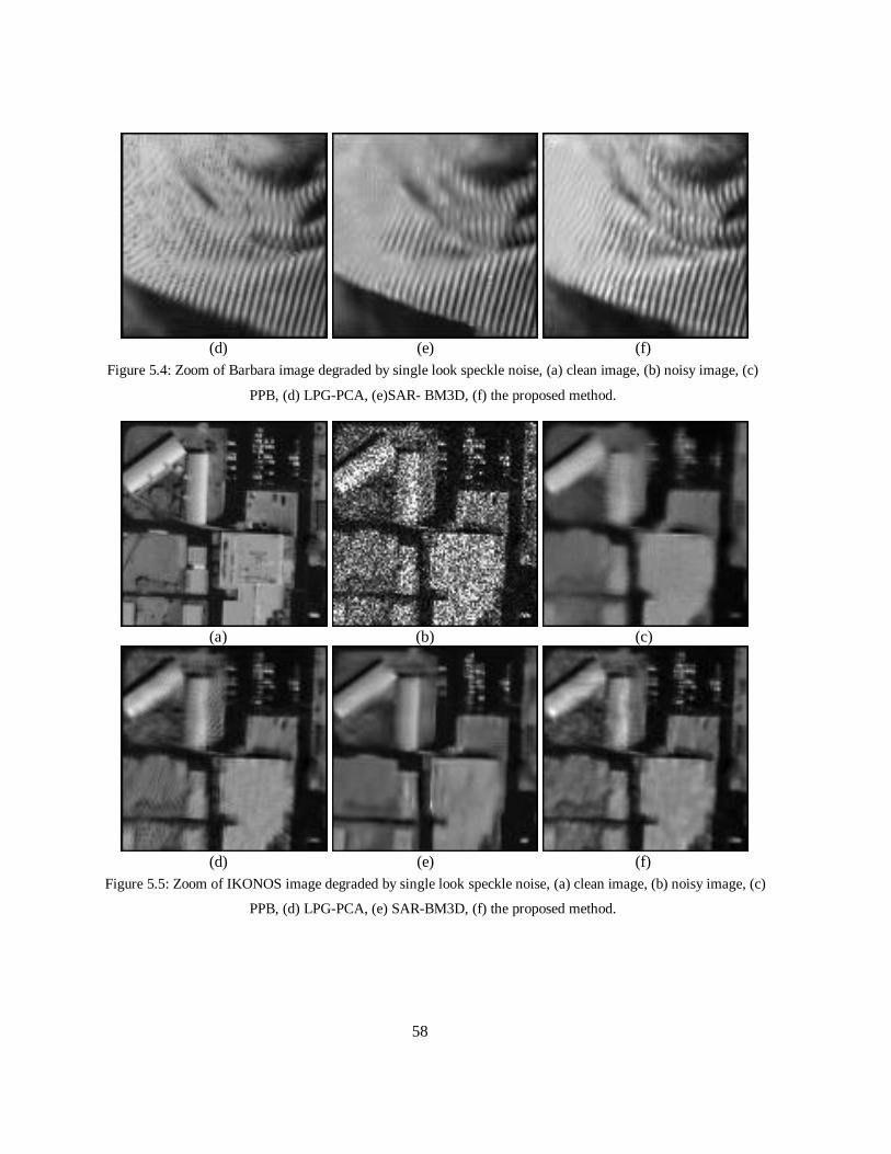
58
(d) (e) (f)
Figure 5.4: Zoom of Barbara image degraded by single look speckle noise, (a) clean image, (b) noisy image, (c)
PPB, (d) LPG-PCA, (e)SAR- BM3D, (f) the proposed method.
(a) (b) (c)
(d) (e) (f)
Figure 5.5: Zoom of IKONOS image degraded by single look speckle noise, (a) clean image, (b) noisy image, (c)
PPB, (d) LPG-PCA, (e) SAR-BM3D, (f) the proposed method.
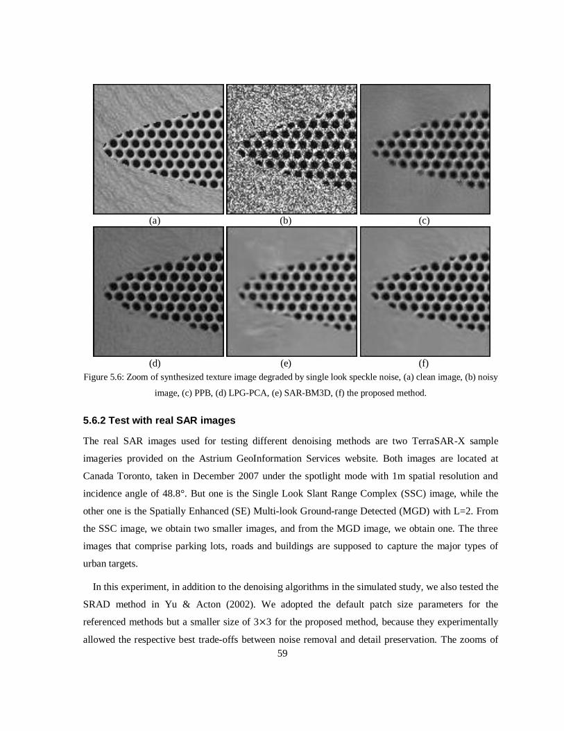
59
(a) (b) (c)
(d) (e) (f)
Figure 5.6: Zoom of synthesized texture image degraded by single look speckle noise, (a) clean image, (b) noisy
image, (c) PPB, (d) LPG-PCA, (e) SAR-BM3D, (f) the proposed method.
5.6.2 Test with real SAR images
The real SAR images used for testing different denoising methods are two TerraSAR-X sample
imageries provided on the Astrium GeoInformation Services website. Both images are located at
Canada Toronto, taken in December 2007 under the spotlight mode with 1m spatial resolution and
incidence angle of 48.8°. But one is the Single Look Slant Range Complex (SSC) image, while the
other one is the Spatially Enhanced (SE) Multi-look Ground-range Detected (MGD) with L=2. From
the SSC image, we obtain two smaller images, and from the MGD image, we obtain one. The three
images that comprise parking lots, roads and buildings are supposed to capture the major types of
urban targets.
In this experiment, in addition to the denoising algorithms in the simulated study, we also tested the
SRAD method in Yu & Acton (2002). We adopted the default patch size parameters for the
referenced methods but a smaller size of 3 3 for the proposed method, because they experimentally
allowed the respective best trade-offs between noise removal and detail preservation. The zooms of
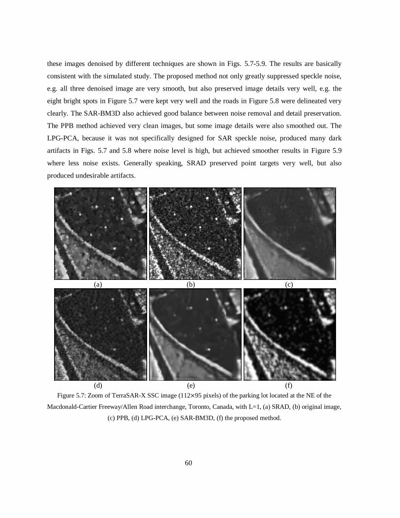
60
these images denoised by different techniques are shown in Figs. 5.7-5.9. The results are basically
consistent with the simulated study. The proposed method not only greatly suppressed speckle noise,
e.g. all three denoised image are very smooth, but also preserved image details very well, e.g. the
eight bright spots in Figure 5.7 were kept very well and the roads in Figure 5.8 were delineated very
clearly. The SAR-BM3D also achieved good balance between noise removal and detail preservation.
The PPB method achieved very clean images, but some image details were also smoothed out. The
LPG-PCA, because it was not specifically designed for SAR speckle noise, produced many dark
artifacts in Figs. 5.7 and 5.8 where noise level is high, but achieved smoother results in Figure 5.9
where less noise exists. Generally speaking, SRAD preserved point targets very well, but also
produced undesirable artifacts.
(a) (b) (c)
(d) (e) (f)
Figure 5.7: Zoom of TerraSAR-X SSC image (112 95 pixels) of the parking lot located at the NE of the
Macdonald-Cartier Freeway/Allen Road interchange, Toronto, Canada, with L=1, (a) SRAD, (b) original image,
(c) PPB, (d) LPG-PCA, (e) SAR-BM3D, (f) the proposed method.

61
(a) (b) (c)
(d) (e) (f)
Figure 5.8: Zoom of TerraSAR-X SSC image (126 116 pixels) of the roads located at the SE of the
Macdonald-Cartier Freeway/Allen Road interchange, Toronto, Canada, with L=1, (a) SRAD, (b) original image,
(c) PPB, (d) LPG-PCA, (e) SAR-BM3D, (f) the proposed method.
(a) (b) (c)

62
(d) (e) (f)
Figure 5.9: Zoom of TerraSAR-X MGD SE image (104 101 pixels) of the area located at 1077 Wilson Ave,
Toronto, Canada, with L=2.1, (a) SRAD, (b) original image, (c) PPB, (d) LPG-PCA, (e) SAR-BM3D, (f) the
proposed method.
5.7 Conclusion
In this chapter, we have presented a SAR images denoising scheme based on clustering the noisy
image into disjoint local regions and denoising each region by LMMSE filtering in PCA domain. In
the clustering step, in order to reduce dimensionality and resist the influence of noise, we identified
several leading PCs in logarithmic domain by MDL criterion to feed the K-means algorithm. This
clustering approach can be treated as the unsupervised counterpart of the commonly adopted block-
matching approach. It requires less computation. Moreover, it is capable of adaptively identifying
―similar‖ patches by considering the closeness to different clusters centers. In the denoising stage, in
order to avoid the limitations of the homomorphic approach, we built our denoising scheme on ASDN
and derived a PCA-based LMMSE denoising model for multiplicative noise. Our approach is the first
to build the PCA-based denoising method on the ASDN model for SAR image denoising. Besides
SAR images, it is also applicable to other signal-dependent noise. The denoised patches of all clusters
were finally used to reconstruct the noise-free image. We tested our denoising scheme in both real
and simulated SAR image with several other state-of-the-art methods. The results suggested that our
method compared favorably w.r.t. the referenced methods in terms of both image detail preservation
and speckle noise reduction.

63
Chapter 6
Conclusions and Recommendations
6.1 Summary and Contribution
This thesis systematically studies MLVM for modeling and analysis of remote sensing data. First of
all, a framework is introduced to provide guidelines for building MLVMs, from a comparative
perspective with mixture models and LVMs. The essence of MLVMs is to model simultaneously two
key factors in remote sensing data generation, i.e. the source heterogeneity effect and the hidden
signals effect, with mixture components discriminating different spatial processes, and latent
dimensions addressing hidden signals in each component. The optimization scheme based on EM
algorithm is described, and specifications of the framework for building task-dependent MLVM
variants are discussed.
Secondly, a MPSR model is proposed for supervised hyperspectral classification, considering the
gap that while SR is an emerging and powerful technique for hyperspectral feature extraction, there is
still a lack of a probabilistic mixture model for it. In order to account for the spatial correlation effect
in labels, a MRF label prior is adopted to be combined with MPSR in a Bayesian framework. The
image classification based on MPSR model is achieved by solving a MAP problem in E-step of EM
iteration. The capabilities of the proposed method are proven in several benchmark hyperspectral
images of both agricultural and urban areas, by comparing with the advanced hyperspectral image
classification method. Besides hyperspectral image classification, MPSR may also be applicable to
other spatial classification issue involving high-dimensional features.
Thirdly, a K-P-Means model is proposed for addressing spectral unmixing issue. K-P-Means aims
to learn nonnegative latent variables in nonnegative latent space, in order to account for the
particularities of remote sensing spectral observations. By imposing label information on latent
variables, K-P-Means model offers a novel interpretation of spectral unmixing. The optimization of
K-P-Means model is achieved by alternating the E- and M-step until convergence. Experiments using
both simulated and real spectral images show that the proposed K-P-Means model provides strong
endmember and abundance estimation results compared to existing approaches. Besides its
application in remote sensing, K-P-Means may also feasible for addressing other nonnegative data
factorization issues or clustering issues in other fields.
64
Lastly, a clustering-based PCA model is designed for advanced SAR image denoising. In this
model, the noise satisfies a Gamma distribution, in order to account for the particularities of SAR
speckle noise. The optimization of this model involves two EM iterations. When learning labels in E-
step, to reduce dimensionality and resist the influence of noise, several leading PCs in logarithmic
space, identified by the MDL criterion are used to feed the K-means clustering algorithm. In M-step,
after learning PCA for each cluster, denoising is achieved by performing LMMSE in PCA domain
based on ASDN model. The experiments demonstrate that the proposed algorithm achieved better
performance than the referenced state-of-the-art methods in terms of both noise reduction and image
details preservation. Besides its application in SAR image denoising, the clustering-based PCA model
may also provide a strong image representation scheme.
The main findings of this thesis are summarized into the following aspects:
(1) MLVM benefits remote sensing data processing, in terms of providing a sound data modeling
framework, which is capable of capture key characteristics of remote sensing data, i.e. the underlying
spatial processes and hidden signals. The theoretical benefits of MLVM are proved by the
successfully application of three MLVMs in addressing different aspects of remote sensing data
processing tasks.
(2) The MLVM is capable of achieving better remote sensing image classification than mixture
models, considering that representing classes by discriminative signals in latent space, is more
effective than characterizing classes by a certain parametric probabilistic distribution in original space.
This conclusion is well justified by the higher classification accuracy achieved by MPSR in
hyperspectral image classification, than an advanced method called MLRsubMLL, which has been
demonstrated higher accuracy than mixture models such as QDA and LDA (Li et al., 2012).
(3) The MLVM is capable of addressing efficiently the spectral source separation issue, which is of
fundamental importance in remote sensing data analysis, by simply adopting the idea of associating
each hidden variable with a mixture component. This capability is well supported by the simplicity,
higher accuracy and lower computational cost achieved by K-P-Means in spectral unmixing.
(4) As far as learning latent variables for image representation is concerned, MLVM also
constitutes powerful technique, due to its ability to capture local structures in feature space. For
example, in representational tasks, i.e. denoising, clustering-based PCA, which follows the key ideas
of MLVM, achieves the state-of-the-art SAR denoising performance, mainly due to the fact that local
65
PCA learnt for individual classes is more capable of achieving noise-discriminative latent variable,
than global PCA learnt for all classes.
In summary, the contributions of this thesis include:
(1) Introduce a probabilistic framework for modeling and estimating both source heterogeneity
effect and hidden signals in remote sensing data. Under this framework, three MLVMs are
successfully developed and applied to different remote sensing applications.
(2) introduce a novel mixture of probabilistic sparse representation (MPSR) model and successfully
integrate it with MRF label prior in Bayesian framework for hyperspectral image classification.
(3) introduce the concept of ―K purified means‖, based on which a novel model called K-P-Means
is developed for spectral endmember extraction.
(4) introduce a clustering-based PCA model for achieving state-of-the-art SAR images denoising
method.
(5) demonstrate in experiments the effectiveness of the proposed models when comparing with the
state-of-the-art methods in their respective applications.
(6) the proposed models are not limited to the demonstrated applications, but can possibly applied
to applications in other disciplines.
6.2 Recommendations for Future Research
6.2.1 Incorporating Label Prior
In remote sensing data, the spatial correlation effect is substantial. Pixels that are spatially close to
each other tend to assume similar labels. Therefore, it is very important to account for this effect in
model building and optimization stage. Nevertheless, of the three proposed models, only MPSR
adopts MRF label prior, in order to remove undesirable artifacts and achieve semantically meaningful
classification results. The reason for not employing label prior in K-P-Means and clustering-based
PCA is mainly because they are designed for learning representative latent variables, instead of for
learning semantically meaningful labels. Nevertheless, it is still worthwhile to explore the outcome of
the two models if the label prior was incorporated, considering that the spatial correlation effect may
have an indirect influence on the latent variable learning.
66
6.2.2 Estimating Hyperparameters
Since MLVM involves both mixture model and LVM, it assumes more hyperparameters than both
sub-models. The hyperparameters in MLVM include the number of classes, the number of latent
bases, the number of active latent variables (e.g. the sparsity in SR) and the structure of the
covariance matrix of noise. In supervised classification or latent variable learning, these
hyperparameters determines directly the model generalization capability. The tuning of
hyperparameters in supervised scenario can be achieved based on posterior information, by cross-
validation techniques (Hastie et al., 2001). In unsupervised cases, although models are not designed
for prediction, it is still crucial to estimate the hyperparameters, in order to achieve meaningful
pattern discovery. The adjusting of hyperparameters can be achieved in Bayesian framework, by
assuming prior distributions for hyperparameters. The resulting model can be solved by certain
optimization techniques, such as variational Bayesian methods (Attias, 1999).
6.2.3 Unsupervised MPSR for Clustering and Latent Variable Learning
In this thesis, although MPSR is used for supervised spectral classification, it also has potential to be
used for unsupervised classification and latent variable learning. Therefore, it is meaningful to
explore the performance of MPSR on spectral clustering, by adopting some dictionary learning
techniques, such as K-SVD, to learn dictionaries for different classes in M-step of EM iterations. It is
also of great interests of to investigate on the capability of MPSR to learn representative latent signals
for some other tasks, e.g. denoising. Note that clustering and latent variable learning can be achieved
simultaneously by solving an unsupervised MPSR model, in which the labels and latent variables will
be estimated iteratively by alternating the E- and M-step until convergence.
6.2.4 K-P-means for clustering
Although K-P-Means is mainly used in this thesis for learning latent variables, i.e. the endmembers, it
is innately a clustering algorithm, where a cluster is represented by an endmember that admits
dominant abundances on the associated pixel in that cluster. Although K-P-Means is capable of
providing a map of dominant endmembers, it could not provide maps of different land cover types,
because a land cover type always involves multiple endmembers. Therefore, in order to adapt K-P-
Means for spectral image segmentation, the concept of cluster in K-P-Means has to be modified to
allow the representation of a class by multiple endmembers, as opposed to by just one. Another
necessary modification is to prescribe the class membership of endmemebrs. Accordingly, in E-step,

67
the representation error over different groups of endmembers will be used to infer the label of spectral
pixel; in M-step, some techniques that allow the learning of multiple endmembers, such as VCA, can
be used to update the endmemebers for each class based on the label information of pixels.
6.2.5 K-P-Means for non-negative matrix factorization
By learning nonnegative latent variables in nonnegative latent space, K-P-Means amount to a
nonnegative matrix factorization techniques, where a data matrix is decomposed into two nonnegative
matrices, in order to learn meaningful patterns. Therefore, it is meaningful to explore the feasibility of
using K-P-Means for addressing some nonnegative data representation issue, in a comparative
perspective with typical nonnegative matrix factorization techniques.
68
References
Achim A., Tsakalides P., and Bezarianos A. (2003). SAR image denoising via Bayesian wavelet
shrinkage based on heavy-tailed modeling. IEEE Transactions on Geoscience and Remote
sensing, 41(8), 1773–1784.
Aharon M., Elad M., and Bruckstein A. (2006). K-SVD: An algorithm for designing overcomplete
dictionaries for sparse representation. IEEE Transactions on Signal Processing, 54(11), 2-4.
Amato U., Antoniadis A., Cuomo V., Cutillo L., Franzese M., Murino L., and Serio C. (2008).
Statistical cloud detection from SEVIRI multispectral images. Remote Sensing of
Environment, 112(3), 750-766.
Argenti F. and Alparone L. (2002). Speckle removal from SAR images in the undecimated wavelet
domain. IEEE Transactions on Geoscience and Remote Sensing, 40, 2363-2374.
Argenti F., Bianchi T., and Alparone A. (2006). Multiresolution MAP despeckling of SAR images
based on locally adaptive generalized Gaussian pdf modeling. IEEE Transactions on Image
Processing, 15(11), 3385–3399.
Argenti F., Bianchi T., and Alparone A. (2008). Segmentation-based MAP despeckling of SAR
images in the undecimated wavelet domain. IEEE Transactions on Geoscience and Remote
Sensing, 46(9), 2728–2742.
Attias, H. (1999, July). Inferring parameters and structure of latent variable models by variational
Bayes. In Proceedings of the Fifteenth conference on Uncertainty in artificial intelligence (pp.
21-30). Morgan Kaufmann Publishers Inc..
Bagon S. (2006). Matlab wrapper for graph cut. [Online]. Available:
http://www.wisdom.weizmann.ac.il/~bagon
Bailey, T. L. and Elkan, C. (1994). Fitting a mixture model by expectation maximization to discover
motifs in biopolymers. International Society for Computational Biology, 2, 28-36.
Bell A. and Sejnowski T. (1995). An information-maximization approach to blind separation and
blind deconvolution. Neural Computation, 7(6), 1129-1159.

69
Bhuiyan M., Ahmad M., and Swamy M. (2007). Spatially adaptive wavelet based method using the
cauchy prior for denoising the SAR images. IEEE Transactions on Circuits and Systems for
Video Technology, 17(4), 500–507.
Bioucas-Dias J. M., Plaza A., Dobigeon N., Parente M., Du Q., Gader P., and Chanussot J. (2012).
Hyperspectral unmixing overview: Geometrical, statistical, and sparse regression-based
approaches. IEEE Journal of Selected Topics in Applied Earth Observations and Remote
Sensing, 5(2), 354–379.
Bioucas-Dias J. M., Plaza A., Camps-Valls G., Scheunders P., Nasrabadi N., and Chanussot J. (2013).
Hyperspectral remote sensing data analysis and future challenges. IEEE Geoscience Remote
Sensing Magazine, 1(2), 6–36.
Bishop C. (2006). Pattern Recognition and Machine Learning. Springer.
Boykov Y., Veksler O., and Zabih R. (2001). Efficient approximate energy minimization via graph
cuts. IEEE Transactions on Pattern Analysis and Machine Intelligence, 20(12), 1222–1239.
Brenning A. (2009). Benchmarking classifiers to optimally integrate terrain analysis and multispectral
remote sensing in automatic rock glacier detection. Remote Sensing of Environment, 113(1),
239-247.
Bryt O. and Elad M. (2008). Compression of facial images using the K-SVD algorithm. Journal of
Visual Communication and Image Representation, 19, 270–283.
Buades A., Coll B., and Morel J. M. (2005). A review of image denoising algorithms, with a new one.
Multiscale Modeling and Simulation, 4(2), 490–530.
Camps-Valls G., Shervashidze N, and Borgwardt K. M. (2010). Spatio-spectral remote sensing image
classification with graph kernels. IEEE Geoscience and Remote Sensing Letters, 7(4), 741-
745.
Camps-Valls G., Tuia D., Gómez-Chova L., Jiménez S., and Malo J. (2011). Remote Sensing Image
Processing. San Rafael, CA: Morgan and Claypool.
Camps-Valls G., Tuia D., Bruzzone L., and Atli Benediktsson J. (2014). Advances in hyperspectral
image classification: Earth monitoring with statistical learning methods. Signal Processing
Magazine, IEEE, 31(1):45–54.
70
Castrodad A., Xing Z., Greer J., Bosch E., Carin L., and Sapiro G. (2011). Learning discriminative
sparse representations for modeling, source separation, and mapping of hyperspectral
imagery. IEEE Transactions on Geoscience and Remote Sensing, 49(11), 4263–4281.
Chang C.-I and Heinz D. C. (2000). Constrained subpixel target detection for remotely sensed
imagery. IEEE Transactions on Geoscience and Remote Sensing, 38(3), 1144–1159.
Chen Y., Nasrabadi N. M., and Tran T. D. (2011). Hyperspectral image classification using
dictionary-based sparse representation. IEEE Transactions on Geoscience and Remote
Sensing, 10, 3973–3985.
Chen Y., Nasrabadi N. M., and Tran T. D. (2013). Hyperspectral image classification via kernel
sparse representation. IEEE Transactions on Geoscience and Remote sensing, 51(1), 217-231.
Chen C., Tang P, and Wu H. (2013). Improving classification of woodland types using modified
priorprobabilities and Gaussian mixed model in mountainous landscapes. International
Journal of Remote Sensing, 34(23), 8518-8533.
Clark R. N., Swayze G. A., Gallagher A., King T. V., and Calvin W. M. (1993). The U.S. Geological
Survey Digital spectral library: Version 1: 0.2 to 3.0µm. USGS, Washington, DC, Open File
Rep. 93-592. U.S. Geological Survey, 1340 pp.
Clark M. L., Roberts D. A., and Clark D. B. (2005). Hyperspectral discrimination of tropical rain
forest tree species at leaf to crown scales. Remote Sensing of Environment, 96, 375-398.
Coupé P., Hellier P., Kervrann C., and Barillot C. (2008). Bayesian nonlocal means-based speckle
filtering. in Proceedings of IEEE International. Symposium on Biomedical Imaging: From
Nano to Macro (ISBI’08), pp. 1291–1294.
Dabov K., Foi A., Katkovnik V., and Egiazarian K. (2007). Image denoising by sparse 3D transform-
domain collaborative filtering. IEEE Transactions on Image Processing, 16(8), 2080–2095.
Dai W. and Milenkovic O. (2009). Subspace pursuit for compressive sensing signal reconstruction.
IEEE Transactions on Information Theory, 55(5), 2230-2249.
Dempster, A.P.; Laird, N.M.; Rubin, D.B. (1977). Maximum Likelihood from Incomplete data via the
EM algorithm. Journal of the Royal Statistical Society, Series B 39 (1): 1–38.

71
Deledalle C., Denis L., and Tupin F. (2009). Iterative weighted maximum likelihood denoising with
probabilistic patch-based weights. IEEE Transactions on Image Processing, 18(12), 2661–
2672.
Deng H. and Clausi D. A. (2005). Unsupervised segmentation of synthetic aperture radar sea ice
imagery using a novel Markov random field model. IEEE Transactions on Geoscience and
Remote Sensing, 43(3), 528–538.
Ding, C., & He, X. (2004, July). K-means clustering via principal component analysis. In
Proceedings of the twenty-first international conference on Machine learning (p. 29). ACM.
Elad M. and Aharon M. (2006). image denoising via sparse and redundant representation over learned
dictionaries. IEEE Transactions on Image Processing, 15(12), 3736-3745.
Fokoue E., and Titterington D. (2003). Mixture of factor analysers Bayesian estimation and inference
by stochastic simulation. Machine Learning, 50(1-2), 73-94.
Frappart F., Ramillien G., Leblanc M., Tweed O. S., Bonnet M., and Maisongrande P. (2011). An
independent component analysis filtering approach for estimating continental hydrology in
the GRACE gravity data. Remote Sensing of Environment, 115, 187-204.
Wang, Y. (2010). Quantitative remote sensing inversion in earth science: theory and numerical
treatment, In: Freeden W., Nashed M. Z., Sonar T. (Eds.), (2010), Handbook of
Geomathematics, Springer. Chapter 26, pp. 787-810.
Frey B. J., Colmenarez A., and Huang T. S. (1998). Mixture of local linear subspaces for face
recognition. Proceedings of IEEE Conference on Computer Vision and Pattern Recognition,
pp. 32-37.
Frey, B. J., Colmenarez, A., & Huang, T. S. (1998). Mixtures of local linear subspaces for face
recognition. In Proceedings of IEEE Computer Society Conference on Computer Vision and
Pattern Recognition June, 1998, pp. 32-37.
Frost V. S., Stiles J. A., Shanmugan K. S., and Holtzman J. C. (1982). A model for radar images and
its application to adaptive digital filtering of multiplicative noise. IEEE Transactions on
Pattern Analysis and Machine Intelligence, PAMI-4(1), 157-166.

72
Gagnon, L., & Jouan, A. (1997). Speckle filtering of SAR images: a comparative study between
complex-wavelet-based and standard filters. In Optical Science, Engineering and
Instrumentation, International Society for Optics and Photonics. October, 1997, pp. 80-91.
Geman S. and Geman D. (1984). Stochastic relaxation, Gibbs distribution, and the Bayesian
restoration of images. IEEE Transactions on Pattern Analysis and Machine Intelligence,
PAMI-6(6), 721–741.
Ghahramani, Z., & Hinton, G. E. (1996). The EM algorithm for mixtures of factor analyzers (Vol. 60).
Technical Report CRG-TR-96-1, University of Toronto.
Guo H., Odegard J. E., Lang M., Gopinath R. A., Selesnick I. W., and Burrus C. S. (1994). Wavelet
based speckle reduction with application to SAR based ATD/R. in Proceedings of the
International Conference on Image Processing. vol. 1, pp. 75–79.
Guo, H., Odegard, J. E., Lang, M., Gopinath, R. A., Selesnick, I. W., & Burrus, C. S. (1994). Wavelet
based speckle reduction with application to SAR based ATD/R. In Proceedings of IEEE
International Conference on Image Processing, November, 1994. ICIP-94., Vol. 1, pp. 75-79.
Hastie T., Tibshirani R., and Friedman J. (2001). The Elements of Statistical Learning. Springer series
in statistics. Springer, New York.
He Y., Gan T., Chen W., Wang H. (2011). Adaptive denoising by singular value decomposition.
IEEE Signal Processing Letters, 18(4), 215-218.
Hinton G. E., Dayan P., and Revow M. (1997). Modeling the manifolds of images of handwritten
digits. IEEE Transactions on Neural Networks, 8(1), 65-74.
Huete A. R. (1986). Separation of soil-plant spectral mixtures by factor analysis. Remote Sensing of
Environment, 19, 237-251.
Hyperspectral Remote Sensing Scenes. (2013). [Online]. Available:
http://www.ehu.es/ccwintco/index.php/Hyperspectral_Remote_Sensing_Scenes
Ju J., Kolaczyk E. D., and Gopal S. (2003). Gaussian mixture discriminant analysis and sub-pixel
land cover characterization in remote sensing. Remote Sensing of Environment, 84, 550 – 560.
Kim, J., & Grauman, K. (2009, June). Observe locally, infer globally: a space-time MRF for detecting
abnormal activities with incremental updates. In IEEE Conference on Computer Vision and
Pattern Recognition, June, 2009. CVPR 2009. pp. 2921-2928.
73
Kondratyev K., and Pokrovsky O. (1979). A factor analysis approach to optimal selection of spectral
intervals for multipurpose experiments in remote sensing of the environment and earth
resources. Remote Sensing of Environment, 8, 3-10.
Kuan D. T., Sawchuk A. A., Strand T. C., and Chavel P. (1985). Adaptive noise smoothing filter for
images with signal-dependent noise. IEEE Transactions on Pattern Analysis and Machine
Intelligence, PAMI-7(1), 165-177.
Lawson C. L., Hanson R. J. (1974). Solving Least Squares Problems. Prentice-Hall,
Lee J. S. (1980). Digital image enhancement and noise filtering by use of local statistics. IEEE
Transactions on Pattern Analysis and Machine Intelligence, PAMI-2(3), 165-168.
Lewicki M. S. and Olshausen B. A. (1999). A probabilistic framework for the adaptation and
comparison of image codes. Journal Optical Society of America A: Optics Image Science
Vision, 16(7), 1587 –1601.
Li S. (2001). Markov Random Field Modeling in Image Analysis. New York: Springer-Verlag.
Li J., Bioucas-Dias J. M., and Plaza A. (2012). Spectral-spatial hyperspectral image segmentation
using subspace multinomial logistic regression and Markov random field. IEEE Transactions
on Geoscience and Remote Sensing, 5(3), 809-823.
Liang S. (2004). Quantitative Remote Sensing of Land Surfaces. John Wiley & Sons, New York.
Lillesand T. M., Kiefer R. W., and Chipman J. (2008). Remote Sensing and Image Interpretation.
John Wiley & Sons, New York.
Liu J. S., Zhang J. L., Palumbo M. L., and Lawrence C. E. (2003). Bayesian clustering with variable
and transformation selections. In Bayesian Statistics Vol. 7, J. M. Bernardo, M. J. Bayarri, J.
O. Berger, A. P. Dawid, D. Heckerman, A. F. M. Smith and M. West (Eds.), Oxford
University Press, pp. 249 -275.
Liu Y., Li W., and Li Y. (2007). Network Traffic Classification Using K-means Clustering. In Second
IEEE International Multi-Symposiums on Computer and Computational Sciences, 2007.
IMSCCS 2007 August. pp. 360-365.
Lloyd S. (1982). Least squares quantization in PCM. IEEE Transactions on Information Theory,
28(2), 129–137.
74
Lopes A., Nezry E., Touzi R., and Laur H. (1990). Maximum a posteriori speckle filtering and first
order texture models in SAR images. in Proceedings of the International Geoscience and
Remote Sensing Symposium, vol. 3, pp. 2409–2412.
Lu D., and Weng Q. (2007). A survey of image classification methods and techniques for improving
classification performance. International Journal of Remote Sensing, 28 (5), 823–870.
Martín G. and Plaza A. (2011). Region-based spatial preprocessing for endmember extraction and
spectral unmixing. IEEE Geoscience and Remote Sensing Letters, 8(4), 745-749.
McLachlan G., and Peel D. (2000). Finite Mixture Models. New York: Wiley.
Miao L. and Qi H. (2007). Endmember extraction from highly mixed data using minimum volume
constrained nonnegative matrix factorization. IEEE Transactions on Geoscience and Remote
Sensing, 45(3), 765–777.
Mountrakis G., Im J., Ogole C. (2011). Support vector machines in remote sensing: a review. ISPRS:
Journal of Photogrammetry and Remote Sensing, 66, 247–259.
Mott H. (2007). Remote Sensing with Polarimetric Radar. John Wiley & Sons, New York.
Mulder V.L.; de Bruin S.; Schaepman M.E.; Mayr T.R. (2011). The use of remote sensing in soil and
terrain mapping—A review. Geoderma, 162, 1–19.
Muresan D. D. and Parks T. W. (2003). Adaptive principal components and image denoising. in
Proceedings of International Conference on Image Processing, vol. 1, pp. 101-104.
Nascimento J. M. P. and Bioucas-Dias J. M. (2005). Vertex component analysis: A fast algorithm to
unmix hyperspectral data. IEEE Transactions on Geoscience and Remote Sensing, 43(4),
898–910.
Oliver, C. and Quegan, S. (1998). Understanding Synthetic Aperture Radar Images. London: Artech
House.
Ozdogan M. (2010). The spatial distribution of crop types from MODIS data: Temporal unmixing
using Independent Component Analysis, Remote Sensing of Environment, 114, 1190-1204.
Parrilli S., Poderico M., Angelino C. V., Verdoliva L. (2012). A nonlocal SAR image denoising
algorithm based on LLMMSE wavelet shrinkage. IEEE Transactions on Geoscience and
Remote Sensing, 50(2), 606-616.

75
Plaza A., Benediktsson J.A., Boardman J.W., Brazile J., Bruzzone L., Camps-valls G., Chanussot J.,
Fauvel M., Gamba P., Gualtieri A., Marconcini M., Tilton J.C., TriannI G. (2009). Recent
advances in techniques for hyperspectral image processing. Remote Sensing of Environment
113(1), S110–S122.
Pu R., and Landry S. (2012). A comparative analysis of high spatial resolution IKONOS and
WorldView-2 imagery for mapping urban tree species. Remote Sensing of Environment, 124,
516-533.
Richards J. A. and Jia X. (1999). Remote Sensing Digital Image Analysis. An Introduction. Springer-
Verlag, Berlin, Heidelberg, Germany, 3rd edition.
Rissanen J. (1978). Modeling by shortest data description. Automatica, 14, 465-471.
Sattar F., Floreby L., Salomonsson G., and Lövström B. (1997). Image enhancement based on a
nonlinear multiscale method. IEEE Transactions on Image Processing, 6, 888-895.
Shaw G. and Manolakis D. (2002). Signal processing for hyperspectral image exploitation. IEEE
Signal Processing Magazine, 50: 12–16.
Small C. (2012). Spatiotemporal dimensionality and Time-Space characterization of multi-temporal
imagery. Remote Sensing of Environment, 124, 793-809.
Solbø S. and Eltoft T. (2004). Homomorphic wavelet-based statistical despeck-ling of SAR images.
IEEE Transactions on Geoscience and Remote Sensing, 42(4), 711–721.
Thessler S., Sesnie S., Bendana Z.S.R., Ruokolainen K., Tomppo E., and Finegan B. (2008). Using
K-NN and discriminant analyses to classify rain forest types in a Landsat TM image over
northern Costa Rica. Remote Sensing of Environment, 112, 2485–2494.
Tipping M. E. and Bishop C. M. (1999). Mixture of probabilistic principal component analysers.
Neural Computation, 11(2), 443-482.
Tropp J. and Gilbert A. (2007). Signal recovery from random measurements via orthogonal matching
pursuit. IEEE Transactions on Information Theory, 53(12), 4655–4666.
Twomey S. (1977). Introduction to the Mathematics of Inversion in Remote Sensing and Indirect
Measurements, Elsevier Scientific, New York.

76
Ustin S. (2004). Remote Sensing for Natural Resource Management and Environmental Monitoring.
Manual of Remote Sensing, Volume 4. John Wiley & Sons, New York.
Viscarra Rossel R. A., and Chen C. (2011). Digitally mapping the information content of visible–near
infrared spectra of surficial Australian soils. Remote Sensing of Environment, 115, 1443-1455.
Wang B-C. (2008). Digital Signal Processing Techniques and Applications in Radar Image
Processing. John Wiley & Sons, New York.
Wax M. and Kailath T. (1985). Detection of signals by information theoretic criteria. IEEE
Transactions on Acoustics Speech and Signal Processing, 33(2), 387-392.
Wu, C. F. J. (1983). On the Convergence Properties of the EM Algorithm. Annals of Statistics, 11(1):
95–103.
Xia J., Du P., He X. and Chanussot J. (2013). Hyperspectral remote sensing image classification
based on rotation forest. IEEE Geoscience and Remote Sensing Letters, 11(1), 239-243.
Xie H., Pierce L., and Ulaby F. (2002). Despeckling SAR images using a low complexity wavelet
denoising process. in Proceedings of the International Geoscience and Remote Sensing
Symposium, vol. 1, pp. 321–324.
Yang M.-H., and Ahuja, N. (1999). Face detection using a mixture of factor analyzers. In
Proceedings of the 1998 IEEE International Conference on Image Processing (ICIP 99),
Kobe, Japan.
Yu Y. and Acton S.T. (2002). Speckle reducing anisotropic diffusion. IEEE Transactions on Image
Processing, 11, 1260-1270.
Zare A. and Gader P. (2010). PCE: Piecewise convex endmember detection. IEEE Transactions on
Geoscience and Remote Sensing, 48(6), 2620–2632.
Zhang L., Dong W., Zhang D., and Shi G. (2010). Two-stage image denoising by principal
component analysiswith local pixel grouping. Pattern Recognition, 43, 1531-1549.
Zhong H., Xu J., and Jiao L. (2009). Classification based nonlocal means de-speckling for SAR
image. in Proceedings of SPIE Wavelet Applications in Signal And Image Processing, pp.
74950V-74950V.

77
78
Appendix A
List of Publications during PhD Thesis Work
[1] L. Xu, and J. Li, 2014. ―Bayesian classification of hyperspectral imagery based on probabilistic
sparse representation and Markov random field―, IEEE Geoscience and Remote Sensing Letters,
11(4): 823-827.
[2] L. Xu, J. Li, A. Wong and J. Peng, 2014. ―K-P-Means: a clustering algorithm of K
‗purified‗ means for hyperspectral endmember estimation―, IEEE Geoscience and Remote Sensing
Letters, 11(10): 1787-1791.
[3] L. Xu, J. Li, Y. Shu and J. Peng, 2014. ―SAR image denoising via clustering-based principal
component analysis―, IEEE Transactions on Geoscience and Remote Sensing,
doi.10.1109/TGRS.2014.2304298.
[4] L. Xu, J. Li and A. Brenning, 2014. ―A comparative study of different classification techniques
for marine oil spill identification using RADARSAT-1 images―, Remote Sensing of Environment, 141,
14-23.
[5] L. Xu, J. Li, A. Wong, C. Wang, 2014. ―A kernel PCA texture feature for efficient segmentation
of RADARSAT-2 sea ice imagery―, International Journal of Remote Sensing, accepted.

79
Appendix B
Waiver of Copyright
IEEE, the publisher of the three manuscripts adopted in Chapter 3, 4 and 5, allows the reuse of published
papers in thesis without a formal permission (see the following statement from IEEE). Therefore, the
waiver of copyright from IEEE has been achieved by following the requirements below.
Policy Regarding Thesis/Dissertation Reuse, from IEEE Copyright Clearance Center
“The IEEE does not require individuals working on a thesis to obtain a formal reuse license,
however, you may print out this statement to be used as a permission grant:
Requirements to be followed when using an entire IEEE copyrighted paper in a thesis:
1) The following IEEE copyright/ credit notice should be placed prominently in the references: © [year of
original publication] IEEE. Reprinted, with permission, from [author names, paper title, IEEE publication
title, and month/year of publication]
2) Only the accepted version of an IEEE copyrighted paper can be used when posting the paper or your
thesis on-line.
3) In placing the thesis on the author's university website, please display the following message in a
prominent place on the website: In reference to IEEE copyrighted material which is used with permission
in this thesis, the IEEE does not endorse any of [university/educational entity's name goes here]'s products
or services. Internal or personal use of this material is permitted. If interested in reprinting/republishing
IEEE copyrighted material for advertising or promotional purposes or for creating new collective works
for resale or redistribution, please go
tohttp://www.ieee.org/publications_standards/publications/rights/rights_link.html to learn how to obtain a
License from RightsLink.
If applicable, University Microfilms and/or ProQuest Library, or the Archives of Canada may supply
single copies of the dissertation.‖