diet analysis of pacific harbour seals (phoca vitulina

DIET ANALYSIS OF PACIFIC HARBOUR SEALS (PHOCA VITULINA RICHARDSI)

USING HIGH-THROUGHPUT DNA SEQUENCING

by

Austen Clouse Thomas

B.Sc., Western Washington University, 2004

M.Sc., Western Washington University, 2010

A THESIS SUBMITTED IN PARTIAL FULFILLMENT OF

THE REQUIREMENTS FOR THE DEGREE OF

DOCTOR OF PHILOSOPHY

in

THE FACULTY OF GRADUATE AND POSTDOCTORAL STUDIES

(Zoology)

THE UNIVERSITY OF BRITISH COLUMBIA

(Vancouver)

September 2015

© Austen Clouse Thomas, 2015

ii

Abstract

Harbour seals have long been perceived to compete with fisheries for economically valuable fish

resources in the Pacific Northwest, but assessing the amounts of fish consumed by seals requires

estimates of harbour seal diets. Unfortunately, traditional diet analysis techniques cannot provide

the necessary information to estimate the species, life stage, and biomass of key prey (e.g.

salmonids) consumed by seals. I therefore developed a new harbour seal diet analysis

methodology, using scat DNA metabarcoding and prey hard-part analysis to create refined

estimates of salmon in harbour seal diet. I also sought to understand the quantitative potential of

DNA metabarcoding diet analysis (i.e. the relationship between prey biomass proportions and

DNA sequence percentages produced by high-throughput amplicon sequencing of seal scat

DNA).

Analysis of faecal samples (scats) from captive harbour seals fed a constant diet indicated that a

wide range of factors influence the numbers of prey sequences resulting from scat amplicon

sequencing. These biases ranged from preferential amplification of certain prey species DNA, to

sequence quality filtering—in addition to interactions between the various biases. I was able to

apply correction factors derived from tissue mixtures of the species fed to captive seals that

improved prey biomass estimates from DNA, and found that the lipid content of prey fish species

perfectly predicted the magnitude of bias resulting from differential prey digestion. My results

suggest that highly accurate pinniped prey biomass estimates can be attained by applying two

stages of corrections to prey DNA sequence counts. However applying these corrections to the

scats of wild seals is challenging, and requires a complete prey tissue mix library to create

species-specific correction factors for all prey. While I established an approach that could be

applied to wild seals, a thorough statistical evaluation and follow-up feeding studies are needed

to determine if the additional effort is justified for population level diet estimates. Lastly, I

developed a decision tree approach for merging salmon DNA and hardparts data from seal scats

to determine the species and life stages of salmon consumed by seals in the Strait of Georgia,

British Columbia.

iii

Preface

All four data chapters in this thesis are the product of a collaborative effort with other

researchers, including scientists at the Australian Antarctic Division, the Washington Department

of Fish and Wildlife, Point Defiance Zoo and Aquarium, CSIRO Marine and Atmospheric

Research, and the University of British Columbia. While I acknowledge the contributions of all

my coauthors, I would like to specifically mention the contributions of Dr. Bruce Deagle to my

thesis, who contributed substantially to my research by assisting with study designs, data

analysis, and the writing of Chapter 2. Two of the four chapters written as manuscripts have been

published in peer-reviewed journals (see below), and the other two are in preparation for

submission.

Chapter 2. The feeding trial in this chapter was done with collaborators at the Point Defiance

Zoo and Aquarium, based on a study design created by Dr. Deagle and myself. I was responsible

for the sample processing of harbour seal scat samples and the laboratory analysis of Run 1. I

also performed the majority of the data analysis and writing for the first draft manuscript created

from the study. After several rounds of peer review, it became clear that additional analyses were

needed (including a second sequencing run) to complete the publication, at which point Dr.

Deagle took the lead on analyses of the new data. The final accepted publication, which appears

in this thesis as Chapter 2, includes both Dr. Deagle and me as the shared primary authors. Dr.

Simon Jarman facilitated the work at the AAD and provided manuscript edits. Amanda Shaffer

was the primary contact at Point Defiance and coordinated scat collections from the captive

seals. For all chapters Dr. Andrew Trites provided manuscript edits and guidance on study

designs. This chapter was published in Molecular Ecology Resources in 2013:

Deagle BE*, Thomas AC*, Shaffer AK, Trites AW, Jarman SN (2013) Quantifying

sequence proportions in a DNA-based diet study using Ion Torrent amplicon sequencing:

which counts count? Molecular Ecology Resources 13:620-633. [* These authors

contributed equally to the study].

Chapter 3. This study developed during the peer review process of my Chapter 2 manuscript,

after subsequent analyses of the feeding trial data from the Point Defiance harbour seal scats.

The study design, laboratory processing, data analysis and writing of the Chapter 3 manuscript

iv

were primarily done by me, with significant input from Dr. Deagle. Additionally, Dr. Simon

Jarman facilitated the sequencing work at the Australian Antarctic Division and provided

manuscript edits. Dr. Katherine Haman contributed conceptual feedback and data interpretation

with respect to digestive physiology. An external laboratory (SGS Canada Inc.) performed the

proximate composition analysis of seal prey fishes. This chapter was published in a special

edition of Molecular Ecology in 2014:

Thomas AC, Jarman SN, Haman KH, Trites AW, Deagle BE (2014) Improving accuracy

of DNA diet estimates using food tissue control materials and an evaluation of proxies for

digestion bias. Molecular Ecology 23:3706-3718

Chapter 4. The study design for Chapter 4 was primarily created by me, with input from Dr.

Deagle and Dr. Trites. Assistance in the lab was provided by an undergraduate student, Corie

Wilson, who graciously spent many hours grinding up fish tissues with me at the UBC Fisheries

Centre. I coordinated the molecular sample processing in two external genetics labs (Laboratory

for Advanced Genome Analysis, and the UGA Georgia Genomics facility) using protocols

adapted from my work with the Australian research group. The manuscript that I wrote from this

study also went through several major rounds of revision before taking its final form. Paige

Eveson, a statistician at CSIRO, played an integral role in the revision of the manuscript and

produced the mathematical expressions contained in the text of the document. All writing and

bioinformatic analyses were done by me, with edits and revisions provided by Dr. Deagle and

Dr. Trites. This chapter manuscript is in the final stages of preparation and has not yet been

submitted for peer review.

Chapter 5. Countless hours went into the harbour seal scat collections for this study (~120

collection trips), and would not have been possible without the help of numerous volunteers who

assisted me in the field. I did the bulk of the laboratory processing of the scat samples

(preparation for molecular and prey bone analysis), with intermittent assistance from

undergraduate volunteers. Monique Lance at the Washington Department of Fish and Wildlife

performed the morphological identification of prey remains in the seal scat samples – a massive

undertaking in itself. Similar to Chapter 4, the molecular wet lab work was subcontracted to an

outside laboratory, but all work was directly supervised by me, and done using a protocol that I

v

developed for MiSeq sequencing of scat DNA. I performed all bioinformatic and statistical

analyses for the study, with some coding assistance provided by Ilai Karen and Alistair

Blachford. My fellow PhD student Benjamin Nelson contributed conceptual feedback on the

decision tree used to merge data from DNA and prey bone analyses. The writing of the

manuscript was done entirely by me, with edits provided by Dr. Bruce Deagle, Dr. Andrew

Trites, and Dr. Marc Trudel. Similar to Chapter 4, the manuscript created from this chapter is

currently in the final stages of revision and has not yet been submitted for peer review.

Animal care and ethics oversight of all research contained herein was administered by the UBC

Animal Care Committee under permit # A11-0072. I successfully completed the ethics training

requirements of the Canadian Council on Animal Care (CCAC) / National Institutional Animal

User Training (NIAUT) Program (Certificate # 4620-11). In addition, all observations of wild

harbour seals and collection of seal faeces were done under a Department of Fisheries and

Oceans License to Study Marine Mammals for Research Purposes (Permit # MML-2011-10).

vi

Table of contents

Abstract .......................................................................................................................................... ii

Preface ........................................................................................................................................... iii

Table of contents .......................................................................................................................... vi

List of tables.................................................................................................................................. xi

List of figures ............................................................................................................................... xii

List of symbols ..............................................................................................................................xv

Acknowledgements ................................................................................................................... xvii

Dedication ................................................................................................................................... xix

Chapter 1: General introduction ..................................................................................................1

1.1 The need for quantitative harbour seal diet information ................................................. 1

1.2 Methods used to characterize pinniped diets .................................................................. 2

1.3 DNA-based pinniped diet analysis .................................................................................. 4

1.4 Outline of thesis data chapters ........................................................................................ 8

Chapter 2: Quantifying sequence proportions in a DNA-based diet study using Ion Torrent

amplicon sequencing: which counts count? ...............................................................................10

2.1 Summary ....................................................................................................................... 10

2.2 Introduction ................................................................................................................... 10

2.3 Materials and methods .................................................................................................. 13

2.3.1 Overview of genetic analysis .................................................................................... 13

2.3.2 Feeding trials and scat sampling ............................................................................... 13

2.3.3 Amplicon library preparation .................................................................................... 14

vii

2.3.4 Sequencing ................................................................................................................ 16

2.3.5 Bioinformatics........................................................................................................... 17

2.4 Results ........................................................................................................................... 18

2.4.1 Overview of sequence data (Run I+II)...................................................................... 18

2.4.2 Fish species proportions in 39 scats (Run I) ............................................................. 20

2.4.3 Influence of read direction and size cut-off (Run I) ................................................. 21

2.4.4 Tag and MID biases (Run I) ..................................................................................... 24

2.4.5 Quality filtering bias (Run I) ..................................................................................... 27

2.4.6 Interactions (Run I) ................................................................................................... 27

2.4.7 Rerun of subset of samples (Run II) ......................................................................... 28

2.5 Discussion ..................................................................................................................... 29

2.5.1 Sources of bias in amplicon sequence proportions ................................................... 29

2.5.2 Relevance to quantitative DNA diet studies ............................................................. 33

2.6 Conclusions ................................................................................................................... 34

Chapter 3: Improving accuracy of DNA diet estimates using food tissue control materials

and an evaluation of proxies for digestion bias .........................................................................36

3.1 Summary ....................................................................................................................... 36

3.2 Introduction ................................................................................................................... 36


3.3.1 Feeding trial, scat sampling and preservation ........................................................... 41

3.3.2 Preparation of food tissue mixture ............................................................................ 41

3.3.3 Amplicon library preparation .................................................................................... 42

3.3.4 Sequencing ................................................................................................................ 43

viii

3.3.5 Bioinformatics........................................................................................................... 43

3.3.6 Proximate composition analysis of prey species ...................................................... 44

3.3.7 Tissue mix correction factors .................................................................................... 44

3.3.8 Digestion correction factors ...................................................................................... 45

3.3.9 Statistical analyses .................................................................................................... 45

3.4 Results ........................................................................................................................... 47

3.4.1 Sequencing and bioinformatics ................................................................................. 47

3.4.2 Tissue Correction Factors ......................................................................................... 49

3.4.3 Digestion Correction Factors .................................................................................... 50

3.5 Discussion ..................................................................................................................... 52

3.5.1 Food tissue control materials .................................................................................... 53

3.5.2 Proxies for digestion bias .......................................................................................... 56

3.5.3 Applicability to other study systems ......................................................................... 57

3.5.4 Conclusions ............................................................................................................... 58

Chapter 4: Quantitative DNA metabarcoding: improved estimates of species proportional

biomass using correction factors derived from control material ............................................59

4.1 Summary ....................................................................................................................... 59

4.2 Introduction ................................................................................................................... 59


4.3.1 Evaluation of tissue correction factors ...................................................................... 62

4.3.2 Development of a harbour seal prey library ............................................................. 65

4.3.3 Wild harbour seal scat samples ................................................................................. 66

4.3.4 Genetic analysis ........................................................................................................ 67

ix

4.4 Results ........................................................................................................................... 69

4.4.1 Evaluation of tissue correction factors ...................................................................... 69

4.4.2 Seal prey library ........................................................................................................ 74

4.4.3 Applying 50/50 TCFs to seal scats ........................................................................... 77

4.5 Discussion ..................................................................................................................... 77

4.5.1 When to use 50/50 TCFs........................................................................................... 80

4.6 Conclusion .................................................................................................................... 81

Chapter 5: Species and life stage of salmon consumed by harbour seals can be estimated by

combining DNA metabarcoding with morphological analysis of faecal samples ..................83

5.1 Summary ....................................................................................................................... 83

5.2 Introduction ................................................................................................................... 83


5.3.1 Scat collection ........................................................................................................... 85

5.3.2 Prey hardparts Analysis ............................................................................................ 87

5.3.3 DNA metabarcoding diet analysis ............................................................................ 88

5.3.4 Bioinformatics........................................................................................................... 90

5.3.5 Estimating salmon life stages .................................................................................... 91

5.3.6 Comparison to 1980s diet data .................................................................................. 93

5.4 Results ........................................................................................................................... 94

5.5 Discussion ................................................................................................................... 104

5.5.1 Diet analysis methods ............................................................................................. 104

5.5.2 Food habits of harbour seals in estuaries ................................................................ 106

5.5.3 Accuracy of juvenile salmon percentage of seal diet .............................................. 109

x

5.6 Conclusion .................................................................................................................. 112

Chapter 6: General conclusion .................................................................................................113

6.1 Summary of research and findings ............................................................................. 113

6.2 Applying DNA metabarcoding diet analysis in other study systems ......................... 117

6.3 Future directions ......................................................................................................... 118

References ...................................................................................................................................120

Appendices ..................................................................................................................................128

Appendix A Supplementary tables and figures for Chapter 2 ................................................ 128

Appendix B Supplementary tables and figures for Chapter 5 ................................................ 134

xi

List of tables

Table 2.1 Sequence counts and percentages of three fish species recovered from seal scats in two

Ion Torrent sequencing runs. ........................................................................................................ 23

Table 3.1 Accounting of all sequences produced by ion torrent sequencing of the harbour seal

scat amplicon pool and the tissue mix amplicon pool for three prey species (capelin, herring and

mackerel). ...................................................................................................................................... 46

Table 3.2 . Data used in the calculation of Tissue Correction Factors (TCFs) and Digestion

Correction Factors (DCFs). ........................................................................................................... 47

Table 3.3 Proximate composition analysis results for the three prey fish in the feeding trial,

displaying mean percentages and standard errors. ........................................................................ 50

Table 5.1 Diets of harbour seals (%) stratified by sampling location (Fraser River, Comox,

Cowichan Bay, Belle Chain), year and season (spring: Apr-Jul; fall: Aug- Nov). ....................... 95

xii

List of figures

Figure 2.1 Schematic showing (a) the combination of multiplex identifier sequence (MID) and

primer tag used to identify amplicons from individual samples. (b) The sample labeling

procedure. ...................................................................................................................................... 15

Figure 2.2 Comparison between proportion of three fish species fed to seals (triangles) versus

overall proportions of sequence reads recovered (box plots). Box plots were generated from the

sequence read proportions from 39 individual scat samples (Run I – 100 bp) using combined

forward and reverse reads. ............................................................................................................ 20

Figure 2.3 Bar plots showing proportions of fish sequences recovered from 39 individual seal

scats in sequenced in Run I (blue= capelin, red = herring, green = mackerel). ............................ 22

Figure 2.4 Mean sequence counts for fish in 39 individual seal scats for various levels of quality

filtering (Run I – 100 bp; forward and reverse reads are shown separately). ............................... 24

Figure 2.5 Plots depicting the interacting effects of three different primer tags (A,B,C) and eight

different quality filter cut-off values on proportions of fish sequences detected in 39 scats (Run I

– 100 bp). ...................................................................................................................................... 25

Figure 2.6 Sequence quality scores vary between species and between (a) forward and (b)

reverse reads. Box plots show summary of mean quality scores (median, range and upper/lower

quartiles across 100 bp of sequence from Run I; n= 110,270 sequences). ................................... 26

Figure 3.1 Overview of the study design and laboratory workflow. ............................................ 40

Figure 3.2 Comparison between mass percentages of three fish species fed to seals ( ) and

sequence percentages obtained from scats ( ) and the tissue mix ( ). .................................... 48

xiii

Figure 3.3 The relationships between the log transformed Tissue Correction Factors (log TCF)

and the percent whole body protein of the prey fish (Left), and between logTCF and the family-

specific percentage of red muscle fibers documented in Greek-Walker& Pull (1974) (Right). ... 49

Figure 3.4 The relationships between the log transformed Digestion Correction Factors (log

DCF) and the proximate composition analysis components of the three prey species (top left = %

lipid, top right = % protein, bottom left = % ash, bottom right = % moisture). ........................... 51

Figure 3.5 The relationship between prey fish lipid content and protein digestibility in harbour

seals. .............................................................................................................................................. 57

Figure 4.1 Six steps involved in calculating tissue correction factors (TCFs) from a prey tissue

library: ........................................................................................................................................... 64

Figure 4.2 (a) Percentage of DNA sequences recovered from tissue mixes of 3 test species (Atka,

capelin, and herring) mixed individually with mackerel (the control species) in ratios of 20:80,

40:60, 50:50, 60:40, and 80:20 by mass. ...................................................................................... 70

Figure 4.3 Proportion of DNA recovered from a) herring mixed with Atka, b) Atka mixed with

capelin, and c) capelin mixed with herring in pairwise ratios of 20/80, 40/60, 50/50, 60/40, and

80/20. ............................................................................................................................................ 71

Figure 4.4 Tissue correction factors applied to DNA sequence percentages obtained from

mixtures of three test species (herring, capelin, and Atka) in the interaction experiment. ........... 72

Figure 4.5 Linear equation for the log transformed proportion-dependent tissue correction factors

(PTCFs), plotted against the 50/50 TCF corrected sequence percentages of all pairwise mixtures

combining test fishes (Herring, Capelin, Atka) with the control fish (Mackerel). ....................... 73

xiv

Figure 4.6 Proportions of DNA sequences counted after Illumina amplicon sequencing of tissue

samples that contained 50% of each test species by mass and 50% chub mackerel (the control

species). ......................................................................................................................................... 75

Figure 4.7 Harbour seal scat samples collected in British Columbia, Canada that were comprised

of only prey species included in our 50/50 tissue library. ............................................................ 76

Figure 5.1 Harbour seal haulouts in the Strait of Georgia, British Columbia, Canada, where scats

were collected. .............................................................................................................................. 86

Figure 5.2 A schematic diagram depicting the decision tree approach we developed to estimate

salmon species and life stage in harbour seal diet. ....................................................................... 92

Figure 5.3 Average diets of harbour seals (%) in estuaries during spring and fall based on

hardparts SSFO percentages (1980s and 2012-2013) and DNA metabarcoding diet percentages

(2012-2013)................................................................................................................................... 98

Figure 5.4 Monthly amounts (%) of juvenile (left) and adult (right) salmon species present in

harbour seal scats collected at haulouts in estuaries (2012-2013). ............................................... 99

Figure 5.5 Percent of adult and juvenile salmon (chum, pink, sockeye, Chinook and coho)

contained in harbor seal scats collected over 4 month periods. .................................................. 100

Figure 5.6 Percentages of salmon (steelhead, sockeye, pink, coho, chum and Chinook) by life

stage (juvenile or adult) in the diets of harbour seals using estuary haulouts in 2012 and 2013.102

Figure 5.7 Estimated fork lengths of juvenile salmon (Chinook, coho and sockeye) derived from

the few otoliths recovered in seal scats that were not too eroded to measure. ........................... 103

Figure 5.8 Comparison of three different methods used to calculate harbour seal population diet

percentages from the same set of scat samples in two different seasons: Spring (when harbour

seals primary eat juvenile salmon); Fall (when harbour seals mostly eat adult salmon). ........... 110

xv

List of symbols

Chapter 3

i A prey fish species in the first tissue mix experiment

TCFi Tissue Correction Factor for species i

DCFi Digestion Correction Factor for species i

Di Mass percentage of species i in the fish tissue mixture

Ti DNA sequence percentage of species i in the tissue mix amplicon pool

Si The percentage of species i detected in the seal scat amplicon pool

Chapter 4

t The test fish species (i.e. the variable fish species in mixtures)

c The control fish species (i.e. the species held constant in all mixtures)

p Percentage of the test fish species in the mixture used to calculate a TCF

TCFp,t Tissue Correction Factor for species t at the given mass percentage p

Mt Mass percentage of the test fish in the mixture

Mc Mass percentage of the control fish in the mixture

St DNA sequence percentage of the test fish species

Sc DNA sequence percentage of the control fish species

N̂t Corrected sequence counts from the sample for species t

Nt Observed sequence counts from the sample for species t

p̂t Corrected DNA percentage of the test fish species in the mixture

xvi

PTCFp Proportion-dependent Tissue Correction Factor for a given proportion p

Proportion-dependent corrected DNA sequence count for species t

Chapter 5

i A harbour seal prey category

SSFOi Split Sample Frequency of Occurrence for prey category i

ω The total number of prey categories

s The number of scat samples in a particular collection

k A specific scat sample in the collection of interest

xvii

Acknowledgements

The names of all of the people who have helped me in the development of this thesis are

simply too many to list. They range from those who contributed technical assistance with

laboratory analysis or bioinformatics, to the many volunteers who spent hours in the field with

me collecting harbour seal scats. I will therefore limit my specific acknowledgments to several

key people who have been integral in the formulation of this thesis.

First, I would like to thank my PhD supervisor, Dr. Andrew Trites, for supporting my

work over the last five years and for encouraging me to pursue a PhD at UBC. I also thank my

thesis committee members, Dr. Carl Walters, Dr. Anthony Sinclair, Dr. Bruce Deagle, and

Monique Lance for their scientific guidance and the many hours spent in committee meetings,

reading thesis chapters, etc. I recognize that their time is highly valuable and I am lucky to have

had such an accomplished group of scientists guiding my work.

I thank my lab mates in the UBC Marine Mammal Research Unit for their scientific and

moral support — all having listened to countless practice talks and offering help in the lab or the

field. I especially thank my fellow PhD student Ben Nelson, who was always enthusiastic to

have another conversation about harbour seals and salmon! Morgan Davies (the MMRU chief

technician) has my undying gratitude for tolerating me for so many years in the scat lab. And of

course, my sincere thanks to our lab manager Pamela Rosenbaum, without whom we would be

but babes lost in the woods.

I owe tremendous gratitude to Dr. Brian Riddell and the Pacific Salmon Foundation for

their exceedingly generous support of my research and graduate degree at UBC. The foundation

fully funded my research and scholarship, in addition to funding my RFID tag project. The latter

in particular was not a low risk venture and I owe them greatly for having faith in my research

ideas.

The marine mammal group at DFO Pacific Biological Station contributed substantially to

my work at UBC. They provided a research vessel for scat collections on Vancouver Island, in

addition to offering much needed historical perspective on seal-salmon interactions in British

Columbia. In addition, Cowichan Tribes contributed to the scat collection efforts in months when

I could not make it over to the island.

xviii

Most importantly I thank my family and my partner, Katie Haman, for always

encouraging me to pursue my curiosity wherever it leads. It takes a special family to be

supportive of an aspiring scientist, and I have been so fortunate to have a family that has done

nothing but support and encourage me along every step of the path. This thesis is as much a

product of their effort as it is mine.

xix

Dedication

For my grandmother, Elizabeth Thomas “Grandma Betty”, whose incredible spirit and boundless

love serves as an inspiration to every person who has been granted the gift of knowing her.

1

Chapter 1: General introduction

1.1 The need for quantitative harbour seal diet information

It is reasonable to assume that as long as humans have observed harbour seals feeding on

adult salmonids at the water’s surface or depredating fishing gear, people have questioned how

many salmon are eaten by harbour seal populations (Lavigne 2003). In 1931, Scheffer and

Sperry wrote of harbour seals in Washington State, “they will rob set nets and have been known

to enter a fish trap, dine on salmon, and escape the way they came in...bringing them into

disfavor with fishermen” (Scheffer and Sperry 1931). Similar statements are made by salmon

fishermen to this day, and likewise by people in all locations where predators are thought to

compete with humans for a common resource.

In the absence of quantitative harbour seal diet information, observations of harbour seals

preying upon salmonids has led to the perception that harbour seals consume large numbers of

economically valuable fish. That perception resulted in the establishment of a seal population

control program that dates back to 1914 in British Columbia, Canada, wherein hunters were

rewarded for turning in the noses of dead harbour seals (Fisher 1952; Olesiuk 2009). Fisheries

managers in the Pacific Northwest have been concerned about the predatory impacts of harbour

seals for over a century, and have responded in the past to public perception of a conflict

between seals and salmon fisheries with dramatic management policies (Jeffries et al. 2003;

Olesiuk 2009).

More recently, fisheries managers have relied on data, as opposed to perceptions, to

inform management actions (Anonymous 1999; Lavigne 2003; Bowen and Lidgard 2013). For

example, if active management of harbour seal populations is deemed necessary in the present

day, it must first be proven by fisheries scientists that seals have a significant negative impact on

fisheries resources (Anonymous 1999). Demonstration of an impact generally involves an

estimate of the numbers of prey consumed by the pinniped population, and an evaluation of seal-

related mortality relative to the prey population abundance and other sources of mortality.

Furthermore, simulation modeling should be used to demonstrate that active management of seal

populations has a relatively high probability of increasing the availability of the targeted fisheries

2

resource to fishers, accounting for potentially complex ecosystem interactions (Punt and

Butterworth 1995; Lessard et al. 2005; Li et al. 2010).

A fundamental component of most pinniped impact assessments is an evaluation of the

pinniped population diet (Bowen and Iverson 2013). Fisheries researchers combine diet estimates

with information about the numerical abundances of the predator species, and the daily energy

requirements of the species, in order to estimate the numbers of individual prey consumed

(Smith et al. 2014). This general framework for creating prey consumption estimates has been

used to estimate the numbers of prey consumed by a variety of marine mammals, including

cetaceans (Lindstrøm 2002), many pinniped species (Ugland et al. 1993; Hammill and Stenson

2000; Winship and Trites 2003), and harbour seals specifically (Olesiuk 1993; Howard et al.

2013).

The accuracy of pinniped consumption estimates is therefore highly influenced by the

accuracy of the methodology used to describe pinniped diet. Without accurate diet information

for the predator suspected of impacting a fishery, it is difficult to assess whether or not that

predator population is in fact influencing fisheries resources. Furthermore, in addition to

numerical accuracy, predator diet information needs to be spatially and temporally appropriate

(i.e. specific to the region and time period of interest) to effectively address resource conflict

questions.

1.2 Methods used to characterize pinniped diets

Numerous methods have been used characterize the diets of seals, and each method has

clear advantages and disadvantages over the alternatives. Marine mammal diet characterization

methods have been thoroughly reviewed previously, and the authors have carefully catalogued

the potential biases associated with each available approach (Tollit et al. 2010; Bowen and

Iverson 2013). My aim is therefore not to repeat their efforts and provide an exhaustive review of

diet methods, but rather to highlight the evolution of pinniped diet analysis techniques and the

rationale for pursuing yet additional alternatives.

The first approach used to characterize the diets of pinnipeds was an analysis of the

stomach contents of lethally harvested animals, which involves identifying prey remains in

3

various stages of digestion, and volumetric analysis of those remains to estimate the relative

proportions of prey in the predator diet (Scheffer and Sperry 1931; Scheffer and Slipp 1944;

Pierce et al. 1989). To this day, stomach contents analysis is arguably the most superior seal diet

analysis technique in terms of the data it can provide, but it has several major disadvantages that

have resulted in it being a less popular research tool (Tollit et al. 2010). The primary

disadvantage being that it requires seals to be killed to provide diet data, or reliance on dead-

stranded animals which may strongly bias population diet estimates. Furthermore, a high

percentage of seal stomachs are empty at the time of harvest, meaning that large numbers of

seals must be killed on multiple occasions to generate a sufficient sample size for seasonal

population diet summaries.

To reduce the impact of diet studies on pinniped populations, researchers turned to the

analysis of seal faecal samples (scats) to characterize population diets (Putman 1984; Dellinger

and Trillmich 1988). Hard prey remains such as fish otoliths recovered from scat samples can be

used to determine the prey taxa consumed, and large numbers of scat samples can be collected

with minimal disturbance to the pinniped population of interest (Olesiuk et al. 1990). An entire

subfield of marine mammal science is now dedicated to the methods involved in the

reconstruction of pinniped diets from hard prey remains (Cottrell et al. 1996; Tollit et al. 1997b;

Tollit et al. 2004; Tollit et al. 2007; Phillips and Harvey 2009).

This subfield developed because numerous factors are known to influence diet summaries

based on prey hard parts in scats; such as the differential passage of prey structures between diet

species (Cottrell et al. 1996), erosion of hard prey remains during digestion that prevents

identification or measurement (Tollit et al. 2004), and selective consumption of prey tissues by

seals that does not include hard structures (e.g. “belly biting”) (Hauser et al. 2008). In addition to

these biases, the mathematical model used to calculate the population diet can also strongly

influence diet estimates, depending on whether it is based on prey biomass reconstruction or a

modified frequency of occurrence. One evaluation of diet methods suggested that the choice of

diet summary metric can lead to an order of magnitude difference in prey species composition of

seal diet (Laake et al. 2002). Taxonomic resolution of prey is also a challenge for hard-parts

methods, with some species structures only being identifiable to the family level (e.g.

Salmonidae).

4

After decades of pinniped diet work focused on morphological hard-parts analysis,

several recent alternative approaches have emerged for diet characterization (Bowen and Iverson

2013). For example, stable isotope signatures detected from pinniped blood or tissue samples can

be used to infer shifts in diet over multiple time scales, and have been applied to identify

important changes in diet associated with life history events for these predators (Germain et al.

2012; Beltran et al. 2015). Stable isotope diet analysis however suffers from low taxonomic

resolution, and most studies are limited to general descriptions of the trophic level at which the

predator feeds (Post 2002; Ben-David and Flaherty 2012). Despite this limitation, stable isotope

analysis continues to be a popular tool among biologists studying the trophic ecology of

pinnipeds (Hobson et al. 1997; Lesage et al. 2001; Zhao et al. 2004; Newsome et al. 2010).

Trophic ecologists have also shown considerable enthusiasm for methods involving diet

descriptions based on fatty acid signatures in animal blubber, milk and blood (Budge et al.

2006). Fatty acids found in animal samples can be related to those contained in potential prey

species, and a statistical model can be applied to infer the most probable diet of the predator

based on possible combinations of the prey species fatty acid signatures (Iverson et al. 2004;

Tollit et al. 2010). Quantitative Fatty Acid Signature Analysis (QFASA) has been used to

characterize the diets of multiple marine mammal species, and has the advantage of high

taxonomic resolution over relatively long time scales — thereby identifying those prey species

that are consistently important for the predator, as opposed to ephemeral prey species simply

present at the time of sampling. Although QFASA was once considered a potential “silver

bullet” for marine mammal trophic ecology, subsequent methodological evaluations have shown

that diet estimates can be highly sensitive to variability in prey species fatty acid signatures

(Nordstrom et al. 2008). This has led to caution among researchers about the interpretation of

diet results produced by QFASA analysis (Grahl-Nielsen 2009; Thiemann et al. 2009).

1.3 DNA-based pinniped diet analysis

Genetic analysis of pinniped scat samples or “molecular scatology” is currently one of

the most promising approaches for characterizing pinniped diets (Deagle et al. 2005; Pompanon

et al. 2012; Clare 2014). DNA based diet methods are highly sensitive (offering a high

5

probability of prey species detection), in addition to providing refined taxonomic assignment of

prey when assays are designed appropriately. Similar to the evolution of pinniped diet analysis as

a whole, DNA based diet analysis methods have also evolved substantially over time.

The first pinniped diet studies to employ DNA focused on improving the taxonomic

resolution of standard hard-parts techniques by extracting DNA from fish bones that could only

be identified to the family level (e.g. salmonids) (Purcell et al. 2000). Species level identification

was enabled using a Polymerase Chain Reaction (PCR) based assay targeting salmon

mitochondrial DNA markers, followed by DNA sequencing of the products or a Restriction

Fragment Length Polymorphism (RFLP) analysis to identify species (Purcell et al. 2004).

Follow-up studies also using salmon bones targeted alternative molecular markers and different

salmon species (Kvitrud et al. 2005; Parsons et al. 2005).

Subsequent genetic diet analysis of pinnipeds has focused on expanding the range of diet

species that can be identified with DNA (using the scat “matrix” and bones), in addition to

exploring the potential quantitative capabilities of DNA-based methods. Around this point in the

evolution of DNA-based diet analysis, the idea of “DNA barcoding” as a means of species

identification began to take hold, and gave rise to the Barcode of Life project (Hebert et al.

2003). DNA barcoding works on the idea that all animals can be identified based on the DNA

sequences of standardized diagnostic genetic markers, similar to the way a supermarket scanner

identifies items using standardized black and white barcodes. Trophic ecologists were quick to

adopt the idea of using standard diagnostic markers to identify prey species in diet samples,

benefiting from a worldwide effort to produce reference databases of species DNA sequences for

barcoding purposes (Jarman et al. 2004).

Where DNA barcoding studies mostly seek to identify individual organisms, DNA diet

analysis usually requires multiple species to be identified from a single diet sample in which the

DNA of multiple food items is present. The latter has been termed “DNA metabarcoding”, i.e.

the simultaneous identification of DNA from multiple organisms in a metasample using standard

DNA barcoding markers (Taberlet et al. 2012a). Alternative terminology has been used in the

past to describe this type of analysis, and because this term was introduced during the

6

development of my thesis, I have also used other terms such as “amplicon sequencing diet

analysis” and “high-throughput sequencing diet analysis” to describe this approach.

The typical DNA metabarcoding diet study today involves PCR amplification of food

species DNA using group-specific primer sets (the target fragment of which provides sufficient

sequence variation to identify food species), followed by high-throughput amplicon sequencing

(a.k.a. next-generation DNA sequencing) (Pompanon et al. 2012). DNA sequences of the target

fragment are then compared to a reference database of species barcodes to determine the food

species present in the diet sample. Similar approaches utilizing clone libraries and Sanger

sequencing, or Denaturing Gradient Gel Electrophoresis (DGGE) were also employed prior to

the widespread availability of high-throughput DNA sequencers (Deagle et al. 2005; Tollit et al.

2009).

Up to this point I have focused on the simple idea of species detection (presence or

absence) of pinniped prey in dietary samples. Presence/absence based models used by ecologists

to estimate the relative biomasses of species consumed by predators have well documented

biases; often overestimating species consumed in low biomass proportion and underestimating

species eaten in large proportion. Several authors have explored the idea of using quantitative

analysis of prey DNA in pinniped scats to better estimate the biomass proportions of the species

consumed. For example, if a direct relationship exists between the relative amount of herring

DNA in a seal scat and the proportional biomass of herring consumed by the seal, a quantitative

DNA approach could have the potential to dramatically improve the accuracy of pinniped diet

estimates.

Two quantitative DNA approaches have been used with scat DNA to estimate the

biomasses of prey consumed by pinnipeds. The first method being real-time or quantitative PCR

(qPCR) targeting specific prey species of animals fed a known diet in a captive setting (Deagle

and Tollit 2007; Bowles et al. 2011), and with samples from wild animals (Matejusová et al.

2008). This approach requires species-specific primers and probes to be developed for all

potential prey, and uses standard curves to estimate the amounts of different prey species DNA

in a sample relative to other prey. The second quantitative approach involves DNA

metabarcoding with group-specific primers, using the percentages of DNA sequences assigned to

different prey as a proxy for the relative biomass of prey consumed. This approach has been used

7

with multiple pinniped species, and amplicon sequences were generated either by clone library or

with high-throughput DNA sequencers (Deagle et al. 2005; Deagle et al. 2009).

Captive feeding trials with sea lions using qPCR to quantify sea lion prey indicated that

prey species DNA proportions are relatively consistent among samples when animals were fed

the same diet. This implies that some relationship exists between prey species DNA % and the

biomass % of prey consumed (Deagle and Tollit 2007; Bowles et al. 2011). However, the prey

species DNA percentages from scats did not match the diet biomass proportions, nor did they

match the species DNA percentages of a tissue mixture created to mimic the diet of the captive

sea lions (Deagle and Tollit 2007). These results suggested that there may be prey species-

specific biases in scat DNA percentages introduced by differential prey digestion, and by

differences in target mitochondrial gene copy number (i.e. variability in the amount of template

DNA in the tissues of different prey species).

One captive feeding study attempted to compensate for copy number differences by

creating correction factors for the ratio of genomic DNA to mitochondrial DNA in different prey

species (Bowles et al. 2011). Numerical correction factors are also routinely employed in

pinniped diet studies using hard parts techniques. Corrections did improve biomass estimates

based on DNA %, but differential prey species digestion was not addressed, and the results were

limited to qPCR studies. DNA metabarcoding approaches are much more flexible than qPCR

(easily detecting many potential prey species without extensive primer design) but are subject to

other potential biases such as difference in primer binding efficiency between species, and

bioinformatic filtering biases.

This foregoing was the state of the field when I began my thesis research. DNA

metabarcoding diet analysis using high-throughput DNA sequencing was a new technique with

exciting potential, and the ability to rapidly produce vast quantities of taxonomic data from

pinniped scats was unprecedented. Overshadowed by the excitement about the technique’s

potential to estimate prey biomass from DNA sequence percentages, was the knowledge that

those percentages are subject to many biasing factors that could potentially influence results.

Therefore I began this work under the perception that the methodological evaluation period

would be brief, and would be followed by extensive study of the foraging behaviors of harbour

seals in the Strait of Georgia, British Columbia. However, the methods portion of my research

8

was not brief, and my efforts followed a lengthy chain of logic in the pursuit of a metaphorical

carrot — the notion that accurate seal prey biomass percentages can be obtained using prey DNA

sequence percentages produced by scat DNA metabarcoding.

1.4 Outline of thesis data chapters

My thesis consists of four data chapters (Chapters 2-5), each written as a standalone manuscript:

Chapter 2. The first data chapter evaluates the potential biasing factors in DNA metabarcoding

diet studies with pinnipeds. The factors evaluated range from the biases introduced by short

DNA sequences attached to PCR primers used to identify individual samples (primer tags), to

biases caused by bioinformatic sequence filtering, and several other biasing factors. The work

stemmed from an in-depth evaluation of the DNA sequences produced from harbour seal scat

samples collected in a captive feeding study at the Point Defiance Zoo and Aquarium. Two

different high throughput sequencing runs were done for the study to a) confirm the sequencing

results from the first run, and b) disentangle the biasing influences of the different factors

evaluated.

Chapter 3. This follow-up study to Chapter 2 contains my initial efforts to devise methods for

correcting seal scat DNA sequence percentages for the various sources of bias, so that they better

represent the biomass percentages of fishes consumed. Working again with the seal scats

produced in the Point Defiance Zoo feeding trial, I tested the applicability of correction factors

based on a fish tissue mix that matched the diet of the seals. I also used proximate composition

analysis of the prey fishes to determine if some compositional property of the prey (e.g. lipid %,

protein %, etc.) could be used as a proxy for the bias introduced by differential prey digestion. I

conclude by postulating how the lessons learned from the study could be applied to scats of wild

harbour seals.

Chapter 4. In this chapter, I explored a promising method to apply tissue-based correction

factors to samples of unknown composition, such as those collected in a wild harbour seal diet

study. Using the approach suggested in Chapter 3, I tested the feasibility of a prey tissue library

of two-species mixtures, wherein one of the two fish species is varied and other fish species is

held constant. This approach is based on the idea that by holding one of the two fish species

9

constant in all mixtures, species specific bias can be inferred based on the variability in DNA

sequences % between mixtures. Furthermore, the prey species biases calculated from these

mixtures can be used to create correction factors for DNA sequence counts in DNA

metabarcoding diet studies. I created a model study system to test the effectiveness of this idea,

in addition to applying 50/50 tissue correction factors to scats of wild harbour seals, based on the

results of a small harbour seal prey library.

Chapter 5. My final data chapter contains an analysis of over 1,000 harbour seal scat samples

collected from estuary seal haulout sites in the Strait of Georgia, British Columbia between 2012

and 2013. In the study, I developed a new method for merging scat DNA information with data

from traditional prey bone analysis to determine the species and age class (juvenile or adult) of

salmon consumed by harbour seals. I combined data from hundreds of scats to describe seal

population diet trends, and then compared it to diet data from the 1980s to detect potential

changes in the ecological role of harbour seals in the Strait. The primary goal of this study was to

produce diet information for harbour seals that can be used to estimate the numbers of juvenile

salmon consumed by harbour seals in the region. To my knowledge, the scatological approach

detailed in this study is the first to provide information sufficient to create pinniped consumption

estimates for salmon that are specific to salmon species and life stage.

10

Chapter 2: Quantifying sequence proportions in a DNA-based diet study

using Ion Torrent amplicon sequencing: which counts count?

2.1 Summary

A goal of many environmental DNA barcoding studies is to infer quantitative information about

relative abundances of different taxa based on sequence read proportions generated by high

throughput sequencing. However, potential biases associated with this approach are only

beginning to be examined. We sequenced DNA amplified from faeces (scats) of captive harbour

seals (Phoca vitulina) to investigate if sequence counts could be used to quantify the seals’ diet.

Seals were fed fish in fixed proportions, a chordate-specific mitochondrial 16S marker was

amplified from scat DNA and amplicons sequenced using an Ion Torrent PGMTM. For a given set

of bioinformatic parameters there was generally low variability among scat samples in

proportions of prey species sequences recovered. However, proportions varied substantially

depending on sequencing direction, level of quality filtering (due to differences in sequence

quality between species), and minimum read length considered. Short primer tags used to

identify individual samples also influenced species proportions. In addition there were complex

interactions between factors; for example, the effect of quality filtering was influenced by the

primer tag and sequencing direction. Re-sequencing of a subset of samples revealed some, but

not all, biases were consistent between runs. Less stringent data filtering (based on quality scores

or read length) generally produced more consistent proportional data, but overall proportions of

sequences were very different than dietary mass proportions indicating additional technical or

biological biases are present. Our findings highlight that quantitative interpretations of sequence

proportions generated via high throughput sequencing will require careful experimental design

and thoughtful data analysis.

2.2 Introduction

The advent of high-throughput sequencing methods allows genetic markers to be characterized at

an unprecedented scale, and has greatly enhanced the scope of studies using DNA-based

identification methods (Valentini et al. 2009b). One area of particular interest is analysis of

species diversity in environmental samples via recovery of many taxonomically informative

11

sequences from DNA mixtures. High-throughput sequencing was initially applied in ecological

studies to characterize microbial taxa (e.g. Sogin et al. 2006), but has been extended into the

realm of eukaryotic organisms including studies focused on microscopic eukaryotes (e.g.

Porazinska et al. 2009; Bik et al. 2012), soil fungal communities (e.g. Buée et al. 2009),

diversity of invertebrate or vertebrate populations (e.g. Hajibabaei et al. 2011; Andersen et al.

2012), and food species in diets of herbivores and carnivores (e.g. Deagle et al. 2009; Valentini

et al. 2009a). These studies used PCR to amplify a variety of different markers and often

employed molecular tagging techniques to distinguish between different strata or individual

samples in order to take advantage of the large amount of data produced by each high-throughput

sequencing run (e.g. Meyer et al. 2007). This enables the analysis of dozens of environmental

samples in parallel, and hundreds or thousands of sequences can be recovered from each to

provide a profusion of data about species diversity.

The goal of many environmental barcoding studies is to infer relative taxon abundance

from proportions of different sequence reads recovered (Amend et al. 2010; Deagle et al. 2010).

However, there are myriad potential biases associated with using sequence counts to quantify

organisms. These include potential biases caused by biological attributes of the target taxa (e.g.

taxon specific variation in DNA copy number per cell, variation in tissue cell density or

differences in environmental persistence). Technical biases can also be introduced at each

laboratory and analytical step. Biases caused by target-specific differences in PCR amplification

have been well scrutinized since a PCR amplification step is also crucial in traditional clone

sequencing approaches (Polz and Cavanaugh 1998; Acinas et al. 2005; Sipos et al. 2007), but

technical biases unique to high-throughput sequencing are just beginning to be evaluated. These

include unavoidable sampling variance between template DNA molecules, but also systematic

biases that cause final sequence counts to deviate from proportions present in template DNA

molecules. For example, it has recently been reported that tagged PCR primers used for

multiplex amplicon sequencing can impact bacterial community profiles obtained through

pyrosequencing (Berry et al. 2011). Another study using pyrosequencing to look at fungal

communities found that sequence count differences between species were due in part to biases

introduced during bioinformatic filtering (Amend et al. 2010). Biases in sequences recovered

12

based on GC content have also been documented from the Ion Torrent sequencer (Quail et al.

2012).

Several dietary DNA barcoding studies have used high-throughput sequencing to

characterize food DNA amplicons recovered from faecal (scat) samples (reviewed in Pompanon

et al. 2012), and in many cases sequence counts have been reported as a semi-quantitative proxy

for diet composition (Deagle et al. 2009; Soininen et al. 2009; Kowalczyk et al. 2011; Murray et

al. 2011; Brown et al. 2012). One study using pyrosequencing found the proportions of four

primary fish prey amplicon sequences recovered from little penguin scats were similar to those

obtained with parallel qPCR analysis, suggesting that sequencing related biases were not large

(Murray et al. 2011). Another study of Australian fur seal diet showed that prey sequence

proportions generated by pyrosequencing were consistent when two different sized mtDNA

barcoding amplicons were used (Deagle et al. 2009). The sequence counts from these studies are

generally presented as fixed values, as in other related fields (e.g. Yergeau et al. 2012), despite

the fact that counts are potentially influenced by many decisions made throughout the

experimental procedure and bioinformatic pipeline (see Amend et al. 2010).

Here we examine count data of fish DNA sequences recovered from scats of captive

harbour seals fed a constant diet. The analysis was carried out using amplicon sequencing on the

Life Technologies Ion Torrent Personal Genome MachineTM (Ion PGM) sequencer (Rothberg et

al. 2011). Our initial objective was simply to see if proportions of prey in diet were reflected in

the proportion of prey sequences recovered; however, our analysis highlighted the fluidity of the

count proportions and led us to examine the influence of experimental factors on the recovered

prey sequence proportions. We specifically considered: (1) sequences obtained from the forward

and reverse read directions, (2) samples marked with different identification tags (added before

or after sample PCR amplification) and (3) data filtered with various levels of quality control

stringency and different minimum read length thresholds. The interactions between these factors

were also considered and a sub-set of samples was re-examined on a second sequencing run to

see if results were congruent.

13

2.3 Materials and methods

2.3.1 Overview of genetic analysis

In the current study a chordate-specific mitochondrial marker (~120 bp) was amplified

from scats of captive seals (targeting the three fish species in their diet) and the amplicons were

examined in two Ion Torrent sequencing runs. Amplicons were labeled with a unique

combination of a 3 bp sequence incorporated onto PCR primers (tag sequences – Tag A, Tag B

or Tag C) and one of 16 different 11 bp multiplex identifier sequences (MIDs) added after PCR

amplification. In Run I, amplicon sequences from 48 scat samples were analyzed and sufficient

data obtained from 39 of these. For this run sequences over 100 bp were considered (Run I - 100

bp) and a parallel analysis included shorter sequences (Run I - 90 bp). In Run II, amplicons from

8 scat samples were analyzed in triplicate (with a different primer tag in each replicate). The

second run was done with newer sequence chemistry and most sequences were >100 bp so one

dataset was considered (Run II – 100 bp). Details are outlined below.

2.3.2 Feeding trials and scat sampling

The feeding trial was carried out with five adult female harbour seals at Point Defiance

Zoo and Aquarium (Tacoma, WA, USA) between July 1 and August 17, 2011. The seals

occupied a single pool, and were fed a constant diet of four species in fixed mass proportions:

capelin (Mallotus villosus ) (40%), Pacific herring (Clupea pallasii) (30%), chub mackerel

(Scomber japonicus ) (15%), and market squid (Loligo opalescens) (15%). Individual species

within daily rations were weighed to the nearest 0.1 kg, and distributed evenly across three meals

in which seals consumed every fish. Daily food intake varied based on seal body mass and their

interest in food, but diet proportions were maintained within measurement precision (2.0% SD

per species; see Table A-1 for a complete record of each animal’s diet).

During the trial, seal scat samples were collected from pool and haul-out areas (generally

within 2-4 hours of deposition), put into Ziploc bags and stored at -20°C. We wanted to

completely homogenize samples since prey DNA is not evenly distributed in pinniped scats

(Deagle et al. 2005). We also wanted to remove all prey hard parts so they did not influence the

genetic data, and to make the protocol useful for studies incorporating parallel hard-part analysis

14

(e.g. Tollit et al. 2009). To accomplish this, our sampling procedure involved transferring thawed

individual scats into a 500 ml plastic container lined with a 124 µm nylon mesh strainer. We

poured 200 ml of 90% ethanol over the scat which was then manually homogenized to form an

ethanol-scat slurry. The strainer was removed along with prey hard parts and the ethanol

preserved scat sediment was stored at -20°C for up to 3 months. DNA extraction was performed

on approximately 20 mg of material using QIAamp DNA Stool Kit (Qiagen) following Deagle et

al. (2005) with elution in 100µl AE buffer.

2.3.3 Amplicon library preparation

The barcoding marker we used was a mitochondrial 16S fragment which is roughly 120

bp in length and has been used previously for differentiating fish species (see Deagle et al.

2009). We amplified this marker with primers Chord_16S_F (CGAGAAGACCCTRTGGAGCT)

and Chord_16S_R_Short (CCTNGGTCGCCCCAAC) which bind to sites that are almost

completely conserved in chordates. Amplicons from the three fish species are within a few base

pairs in length but differ by more than 20% sequence divergence (see Table A-2, Table A-3,

Table A-4 for sequence alignments including primer binding region). Initially we also ran PCRs

with a second primer set which would amplify squid DNA in addition to fish (see Deagle et al.

2009); however, the amplicon length was >250 bp and initial Ion Torrent library preparations

failed (new library preparation procedures now allow sequencing of fragments >400 bp).

Therefore, this marker was abandoned and the squid diet portion excluded from subsequent

analyses. To limit amplification of seal DNA, a 32 bp blocking oligonucleotide (see Vestheim

and Jarman 2008) matching harbour seal sequence was used in PCR (with a modified C3 spacer

at the 3′-end to prevent extension; details in Table A-2). All PCR amplifications were performed

in 20 μl volumes using a Multiplex PCR Kit (QIAGEN). Reactions contained 10 μl master mix,

0.25 μM of each primer, 2.5 μM blocking oligonucleotide and 2 μl template DNA. Thermal

cycling conditions were: 95 °C for 15 min followed by 34 cycles of: 94 °C for 30 s, 57 °C for

90 s, and 72 °C for 60 s. Products were checked on 1.8% agarose gels.

15

Figure 2.1 Schematic showing, (a) the combination of multiplex identifier sequence (MID) and primer tag

used to identify amplicons from individual samples, and (b) the sample labeling procedure. First this involved

PCR amplification of scat template DNA using one of three tagged primer sets (A,B,C). Second, an Ion

Torrent MID was ligated to the amplicons (16 different MIDs), such that all samples received a unique

combination of primer tag and MID.

We prepared amplicon libraries for two Ion Torrent sequencing runs. The first (Run I)

contained equal volumes of DNA amplified from 48 individual scats with each sample being

uniquely labeled (see below). The second (Run II) was a re-analysis of three new PCR

amplifications of DNA from each of 8 scats characterized in the initial run. The purpose of this

Run II was to see if the results (and technical biases) were consistent between runs. Ion Torrent

protocols existing at the time only allowed differentiation of 16 samples, so a two-step sample

tagging process was used to differentiate between amplicons from the 48 individual scat samples

in Run I and the 24 samples in Run II (Figure 2.1).

16

Both tagging approaches are routinely used to differentiate samples in studies employing

high-throughput sequencing platforms. In step 1, short tags added to the 5ˈ end of the primer

were incorporated into amplicons during PCR. In our case, we amplified DNA extracted from

each scat sample using primers containing one of three different 3bp primer tags (Tag A = CAT,

Tag B = GCA, Tag C = TAC; for a given sample both forward and reverse primers had identical

tags).The forward primer contained an additional 3 bp spacer (ATG) after the primer tag. These

tags allowed us to identify 3 groups of PCR amplicons. In step 2 we used the Ion Barcoding 1-16

kit (Life Technologies; part no. 4468654 Rev. B) which ligates up to 16 unique 11 bp multiplex

identifier sequences (MIDs) onto amplicons post-PCR. PCR amplicons containing unique tagged

primers were assigned to one of 16 Ion Torrent MIDs, thus creating 48 unique combinations of

primer tags and MIDs for individual samples in Run I. This tagging scheme was used in part to

evaluate tag specific biases. Individual tagging of samples could also have been achieved using

many uniquely tagged primer sets; however that approach would not allow for replication of

primer tags sufficient to evaluate tag biases. Sequencing Run II was intended in part to decouple

the potential effects of individual sample variability and MID sequence from the effects of

primer tags. In this sequencing run, each of 8 samples was amplified with all three tagged primer

sets, and the MID sequence was kept constant for each sample.

2.3.4 Sequencing

We used the Ion OneTouchTM System (Life Technologies) to prepare amplicons (already

containing MIDs and associated capture and sequencing primers) for sequencing following the

appropriate user’s guide protocol. In the single year that we have been working with the Ion

Torrent system, at least four different sequencing kit upgrades have been released. Therefore, the

two sequencing runs we report here were done with different kits. The first run was performed

using the Ion OneTouch Template kit (p/n 4468660) and the second with the Ion OneTouch™

200 Template Kit v2 (p/n 4478316). The resultant enriched Ion SphereTM particles were loaded

onto 314 Ion semiconductor sequencing chips, and sequencing was carried out on the Ion PGM

sequencer. Bidirectional sequencing was performed (i.e. sequence reads started from forward and

reverse PCR primers), but reads were not paired. Each run was expected to produce

approximately 100,000 reads. For Run I, expected read length was 100 bp (~75 bp being target

17

specific sequence, as this estimate includes the PCR primer and primer tag), so the full 16S

fragment was not covered in a single read. In the second run, due to improved chemistry, reads

were expected to be 200 bp in length which covers the full amplicon.

2.3.5 Bioinformatics

The Ion Torrent platform automatically sorted sequences based on the 16 MIDs, removed

the MID sequence, and output a single FASTQ file for each MID. Quality metrics were based on

reanalysis of raw data carried out at the end of the study with Torrent Suite software version

2.0.1. All post-sequencing analysis (except for taxonomic assignment ; see below) was carried

out using the R language (R 2010) making use of the Bioconductor packages ShortRead (Morgan

et al. 2009) and Biostrings (all relevant FASTQ files and R code are available in Dryad). Our

approach was slightly unconventional in that we kept all of sequences above the cut-off sequence

length in the final database. This included sequences that were low quality, taxonomically

unassigned, and those that did not match a primer. Briefly, the procedure involved importing

FASTQ output files into R, and sequences along with quality information were extracted.

Sequences and quality information were trimmed to 100 bp and data from shorter sequence reads

was discarded. Sequences were exported in FASTA format and prey species assignment was

done using the software package QIIME (Caporaso et al. 2010). In QIIME, a BLAST search for

each sequence (removing tag and start of primer sequence) was done against a local reference

database containing 16S sequences for the three fish species and harbour seal. The match of each

Ion Torrent sequence to reference sequences was assessed based on having a BLASTN e-value

less than a relatively strict threshold value of E < 1e-20 and a minimum identity of 0.9. The

minimum identity score and our pre-defined reference sequences prevented assignment of

chimeric sequences. Resultant species assignments (including a category for sequences with no

blast hit) were imported back into the R workspace. Sequence quality scores for all base calls

were incorporated into the dataset and mean quality scores were calculated. For each sequence,

read direction was determined and sequences were matched to their individual sample of origin

where possible (based on primer sequence, MID number and primer tag). For a sequence to be

linked to a specific sample and read direction, it had to match the 3 bp primer tag and the first 11

bases of the primer (11 bp chosen to avoid a homopolymer run in the reverse primer). This

18

included the ATG spacer sequence in the forward primer, and we allowed for mismatches at two

variable sites in the reverse primer. The resultant dataset, containing all sequences in the original

100 bp FASTQ files and related information, could then be queried based on quality score, read

direction, tag identity, MID identity etc., and sequences tallied based on taxonomic assignments.

In Run I many of the sequences were less than 100 bp in length; thus for comparison, a parallel

dataset was created using a 90 bp size cut-off.

2.4 Results

2.4.1 Overview of sequence data (Run I+II)

The sequencing of Run I (amplicons from 48 individually identifiable scats) produced

330,594 reads with a mean length of 102 bp (33.70 Mbp of data; 23.72 Mbp of Q20 Bases). The

total number of Ion Torrent sequences generated varied considerably among the 16 MIDs (mean

= 18,687, range = 1 – 45,972) with 22,338 sequences unassigned to a MID. The low sequence

counts from some MIDs are likely due to errors made in the course of a complex MID labeling

protocol (pooling of PCR products with different tags within a MID show very even recoveries,

so this step is unlikely to cause these differences). Three of the 16 MIDs were excluded from

further analyses due to low overall sequence counts (< 400 sequences/scat sample). For the

remaining 13 MIDs, representing 39 scat samples, a total of 297,049 sequences were exported

into FASTQ files (mean read number per MID = 22,850; range = 2,206 - 45,972). Out of these

sequences, 63% (n= 188,534) were over 100 bp in length (93% were more than 90 bp in length)

and these were assigned to local reference sequences using BLAST.

For the Run I – 100 bp dataset 70% (n=131,571) of sequences could be linked with a

specific scat sample based on their match with a PCR primer and associated tag. The mean

quality score for sequences matching a primer was 25.0 versus 20.5 for those without a match.

Of the primer matched sequences 84% (n=110,270) were assigned to species in our reference

library based on local BLAST assignation. The vast majority of assigned sequences matched the

three fish species in the seals’ diet, with only 2.3 % (n=2522) identified as harbour seal. While

only sequences with an identified primer and taxonomic assignment were considered in the final

analysis, we also examined the discarded sequences. More than half of the sequences that were

19

excluded because they did not match a primer could be assigned to a prey species (n=30,614)

using our stringent local BLAST. A subset of sequences without taxonomic assignment

(including those without a primer match, or a primer match but no local BLAST match) were

characterized against the full NCBI nucleotide database. The top hit for the majority of these

sequences were feeding trial prey species, but were below the minimum identity (potentially

including chimeric sequences). Most others had no strong matches in the database; however, a

small percentage of sequences matched those from the preceding Ion Torrent sequencing run

(humpback whale nuclear gene amplicons; 0.5 % of 100 bp dataset; n= 971). These

contaminating sequences likely resulted from carry over in the OneTouch instrument used for

emulsion PCR (a new cleaning procedure for maintaining the instrument between runs has since

been implemented by Life Technologies). Overall, results from the Run I - 90 bp dataset were

similar to those reported for the 100 bp dataset and are summarized in supplementary material

(Figure A-1; Figure A-2; Figure A-3; Figure A-4).

A subset of samples was re-sequenced in Run II; these amplicons were from new PCR

amplifications of DNA from 8 scats characterized in the initial sequencing run. DNA from each

scat was amplified in triplicate (once with each set of tagged primers) and amplicons from each

of the 8 samples were labeled with a separate MID sequence. This run with new sequencing

chemistry produced 405,211 reads with a mean length of 151 bp (61.30 Mbp of data; 31.84 Mbp

of Q20 Bases). The total number of Ion Torrent sequences was more consistent between the 8

MIDs used in Run II (mean = 37,010, range = 24,334 – 48,391) with 104,140 sequences

unassigned to a MID. Despite only 8 MIDs being employed in Run II, some sequences were

allotted to each of the 16 potential MIDs. The sequences from 8 unused MIDs represented only

0.6% of sequences (n= 2328; range 6-1415 per MID) and were generally low quality sequences

(100 bp mean =17.6). These sequences primarily matched prey species of this study, and likely

represent rare misassignment of sequences between MIDs rather than contamination since these

amplicons had not been sequenced in the previous 10 runs. Low levels of contaminating

sequences from the previous sequencing run were present (despite using the new OneTouch

cleaning protocol). The contaminants were sheared long-range PCR amplicons (human DNA)

and were apparent since many of the recovered sequences exceeded the maximum size of target

mtDNA amplicons.

20

Figure 2.2 Comparison between proportions of three fish species fed to seals (triangles) versus overall

proportions of sequence reads recovered (box plots). Box plots were generated from the sequence read

proportions from 39 individual scat samples (Run I – 100 bp) using combined forward and reverse reads.

From the 8 correctly classified MIDs a total of 296,079 sequences were exported into

FASTQ files and 96% of these were over 100 bp in length. For the Run II 100 bp dataset, 56%

(n=159,952; mean quality 26.8) could be linked to a specific PCR sample based on the primer;

this percentage was low compared to Run I due to more non-target sequences (without close

blast matches) being recovered. Of sequences which contained primers, 87% (n= 139,630) of

these were assigned to species in our reference library. Harbour seal sequences made up 5.8%

(n=8087) of these assigned sequences.

2.4.2 Fish species proportions in 39 scats (Run I)

The proportion of three fish species consumed in the diet was known, so our initial

objective was to simply see if these proportions were reflected in the sequence counts. Based on

21

previous experiments, we expected relatively low variation in the proportions of prey sequences

amplified from scats of animals fed a consistent diet (Deagle and Tollit 2007; Bowles et al.

2011). If we consider the average composition of 39 scat samples based on all assigned

sequences >100 bp there was little variability in the proportions of sequences assigned to the fish

species (Figure 2.2).

These sequence proportions do not match proportions of the three species consumed.

Capelin was considerably underrepresented (7.3± 3.0% SD versus 48.5% of fish diet), herring

was considerably overrepresented by sequence proportions (74.8± 7.0% SD versus 34% of fish

diet), and mackerel matched the diet (17.9±6.7% SD versus 17.5% of fish diet). The discrepancy

could be caused by many factors (such as PCR bias or biological differences between prey).

However, here our focus is specifically on how choices made throughout the experimental

procedure and during bioinformatic sorting, impact proportions of various species in the

sequence counts.

2.4.3 Influence of read direction and size cut-off (Run I)

Despite forward and reverse DNA strands being present in equimolar amounts after PCR,

sequencing read direction substantially influenced the proportions of sequences assigned to each

fish species (Figure 2.3; Table 2.1).

In the forward read direction, by far the largest percentage of sequences were herring

(85.5% ± 9.5% SD) with very few sequences from mackerel (10.0% ± 7.2% SD) or capelin

(4.5% ± 3.5% SD). In the reverse read direction, proportions of sequences were substantially

different: herring (47.4 ± 17.7 SD), followed by mackerel (39.5 ± 17.1% SD), then capelin (13.1

± 5.6% SD). Sequence counts indicate the differences between forward and reverse reads were

primarily driven by a bias favouring herring fragment reads in the forward direction (Figure 2.4;

Table 2.1).

22

Figure 2.3 Bar plots showing proportions of fish sequences recovered from 39 individual seal scats in

sequenced in Run I (blue= capelin, red = herring, green = mackerel). Each bar represents an individual

sample, and proportions of forward and reverse reads are shown separately. Data were filtered to retain

either sequences >100 bp (top) or >90 bp (bottom). Proportions of three fish species by mass in the diet are

shown as dotted lines on plots.

23

Table 2.1 Sequence counts and percentages of three fish species recovered from seal scats in two Ion Torrent

sequencing runs. Run I data are from 39 scat samples, Run II data are from a subset of these scats (n=8) each

re-run in triplicate with different primer tags (A,B or C). Data are shown for various subsets of recovered

sequences (both without quality filtering and when only sequences with high quality scores are considered).

No quality filter Mean sequence quality >28

Data/Subset Primer Capelin Herring Mackerel Capelin Herring Mackerel

Diet/Fish1 % 48.5 34 17.5

Run I - 100bp2 F % 4.5±3.5 85.5±9.5 10.0±7.2 2.8±2.9 91.5±6.5 5.7±4.7

Mean count5 90 1586 209 25 822 52

R % 13.1±5.6 47.4±17.7 39.5±17.1 15.1±7.8 22.6±22.6 62.3±22.6

Mean count5 121 456 301 47 95 167

Run I - 90bp3 F % 10.8±7.2 76.7±7.9 12.5±4.2 6.5±6.1 83.4±6.3 10.0±3.8

Mean count5 233 1588 276 61 860 107

R % 20.2±8.8 64.0±13.3 15.7±7.9 29.7±17 45.1±26.4 25.1±15.3

Mean count5 440 1348 313 239 394 176

Run II /TagA4 F % 16.7±4.2 68.4±2.6 14.9±4.3 15.8±5 71.9±3.7 12.3±3.6

Mean count5 700 2940 651 425 2034 348

R % 19.2±2.9 64.3±3.7 16.6±6.1 20.9±3.1 64.8±3.7 14.3±5.6

Mean count5 707 2395 628 516 1608 359

Run II /TagB4 F % 13.8±3.6 74.2±3.1 12±3.5 12.5±3.6 79.9±3.5 7.6±2.4

Mean count5 271 1469 238 170 1114 104

R % 14.9±2.9 72±4.4 13.2±4.8 15.8±3.3 72.6±4.9 11.6±4.5

Mean count5 229 1102 200 175 795 126

Run II/TagC4 F % 14.4±3.4 72.4±2.7 13.2±4.1 12.9±3.4 79.5±4.4 7.6±2.9

Mean count5 376 1926 351 231 1476 137

R % 20.4±4 61.1±4.6 18.4±6.5 35.0±11.9 41.0±12.1 24.0±8.7

Mean count5 454 1382 424 333 468 248 1 Percentage composition of fish species in seals’ diet 2 Data from sequencing Run I (amplicons from 39 scats) including only sequences >100 bp in length 3 Data from sequencing Run I including all sequences >90bp in length 4 Data from sequencing Run II, amplicons from 8 scats run in triplicate with different primer tags (A,B or C) 5 Mean number of sequences recovered per sample within data subset

24

Figure 2.4 Mean sequence counts for fish in 39 individual seal scats for various levels of quality filtering (Run

I – 100 bp; forward and reverse reads are shown separately).

The proportions of various sequences recovered were also influence by the arbitrary

sequence length cut-off point used to define the final dataset. When all sequences >90 bp (Run I

– 90 bp) were considered (rather than only those >100 bp), the differences between forward and

reverse reads were less dramatic (Figure 2.3; Table 2.1).

2.4.4 Tag and MID biases (Run I)

In addition to being influenced by read direction, sequence proportions were also

influenced by primer tags added during PCR to trace sequences back to their sample of origin

(Figure 2.5). In the forward read direction a higher proportion of herring DNA fragments were

amplified and sequenced from primers containing Tag A (97.1±4.6 % SD) than from either Tag

B (77.8 ±5.8% SD) or Tag C (81.6±2.7% SD). In the reverse read direction there was more

variation in prey proportions within each tag, but substantial differences between tags were also

apparent (e.g. Herring Tag A: 46.2±17.6% SD; Tag B 37.9±17.8% SD; Tag C 58.1±11.8% SD).

The differences in species composition between tags were not consistent between read

directions, suggesting values do not represent the true differences between samples (Figure 2.5).

25

Figure 2.5 Plots depicting the interacting effects of three different primer tags (A,B,C) and eight different

quality filter cut-off values on proportions of fish sequences detected in 39 scats (Run I – 100 bp). Sequence

proportions for each tag (represented by different shapes) at a given quality score cut-off (varies along the x-

axis) and add up to 1. Results for forward and reverse read directions are displayed separately. Error bars

represent standard error.

26

Figure 2.6 Sequence quality scores vary between species and between (a) forward and (b) reverse reads. Box

plots show summary of mean quality scores (median, range and upper/lower quartiles across 100 bp of

sequence from Run I; n= 110,270 sequences). Line plots show variation in mean quality at positions along the

sequence for each of target species in the same dataset.

In Run II we processed individual samples with different tags to examine the tag effect

further (see below). Only three samples were sequenced with each Ion Torrent MID, so we had

little power to evaluate variability in sequence proportions between MIDs. However, there were

some differences between MIDs that warrant further examination. For example, the length of

sequence reads between MIDS varied slightly; in our analysis only 61% of the sequences from

MID#4 were longer than 100 bp versus 87% of sequences from MID#5. The quality scores also

varied slightly between MIDs. For example, 28% of herring sequences labelled with MID#4 had

27

mean quality scores over 30, versus only 10% labelled with MID#5 (calculated over 100 bp for

both).

2.4.5 Quality filtering bias (Run I)

Data reported up to this point were not quality filtered beyond initial processing by the

Torrent Suite software; however, post-sequencing quality control in amplicon sequencing studies

is generally carried out based on quality scores assigned to sequences. For amplicons in the

current study, sequence quality generally diminished along the length of the read; quality scores

were initially similar between species and then diverged, becoming species-specific as sequences

became different (Figure 2.6).

Particular sequencing positions in both forward and reverse read directions had notably

low quality scores. This was particularly apparent at the start of reads where species share the

same sequence. For example, in the reverse read direction nucleotide quality score dropped

dramatically to its lowest point at sequencing position 15 (mean quality score =18.2). That

position corresponds with the third C in the CCCC homopolymer of the reverse primer. The

majority of these primer sequences were incorrectly called as CCC (even when considering only

higher quality reads in Run I that matched the first 11 bp of the primer and were taxonomically

assigned). Overall, mean sequence quality scores varied between species, and to some degree

with sequencing direction (Figure 2.6). In the forward direction, when quality scores were

averaged over 100 bp, the highest quality sequences overall were herring (mean=27.4) followed

by capelin (mean=25.9) and then mackerel (mean=25.2). For the reverse direction the opposite

trend was observed (Reverse: mackerel = 27.3; capelin = 26.2; herring = 25.0). These species

differences in sequence quality resulted in predictable biases in sequence counts that were

introduced during quality filtering. For example, as quality score cut-off stringency increased for

the reverse reads, more of the relatively higher quality mackerel sequences were present and

fewer of the lower quality herring sequences were retained (Figure 2.5).

2.4.6 Interactions (Run I)

The proportions of sequences assigned to the three species were also affected by

interactions between the factors evaluated in this study (sequencing direction, size cut-off, primer

28

tag, and quality cut-off value; see Figure 2.5). As mentioned above, sequence proportions in the

forward direction responded differently to quality filtering than they did in the reverse direction.

For example, the proportion of mackerel sequences decreased with additional quality filtering in

the forward direction, whereas it increased with stricter quality filtering in the reverse direction.

This effect was smaller in the 90 bp amplicon data set compared to the 100 bp data set (Figure

A-1; Figure A-2).

Sequence proportions also responded differently to the primer tags depending on the level

of quality filtering and read direction. In the forward direction, Tags B and C tended to converge

with Tag A when the level of quality filtering was increased, but Tag A sequence proportions

were virtually unchanged (Figure 2.5). In contrast, in the reverse direction Tag C responded

more strongly to quality filtering that the other two. Again these effects were somewhat

dependent on sequence length cut-off used (Figure A-1; Figure A-2).

2.4.7 Rerun of subset of samples (Run II)

In the absence of quality filtering, the eight re-run samples produced reasonably

consistent results between samples, between the three amplifications with different primer tags,

and between sequencing directions (Table 2.1). These results were in general agreement with

overall results obtained from the 39 scats sequenced in Run I (all assigned sequences >100 bp in

Run II: capelin=16.4± 3.3%; herring= 69.0± 4.4%; mackerel= 14.6±4.7%, compared to data in

Figure 2.2). However, mean values in Runs I and II were produced by quite different underlying

values. For example, in Run I the bias towards herring sequences in the forward read direction

was much stronger compared to Run II (although observed to some extent in both runs; Table

2.1). Direct comparison of 8 individual samples between runs was hampered because in Run I

they were all amplified using primers labelled with Tag A, and these samples had a very large

proportion of herring in the forward direction (Figure 2.5). This Tag A effect was not observed in

Run II, in fact Tag A replicates in Run II had a lower proportion of herring compared to other

tags (individual samples had always had less herring when labelled with Tag A compared to Tag

B, the mean difference was 5.8%). While the tag effect was minor in the second run this bias,

and differences between sequencing directions, became much more substantial with increased

filtering based on quality scores (Table 2.1). Quality filtering had the strongest impact on

29

sequences labelled with Tag C in the reverse direction, similar to the effect seen in Run I. This

three base pair primer tag (TAC) produces a homopolymer of three C’s when combined with the

reverse primer (only two C’s with the other tags). This may explain why samples labelled with

Tag C were more influenced by quality filtering. While the quality of sequences assigned to each

species was generally higher in Run II compared to Run I this was not the case for mackerel

reverse read sequences. The lower relative quality of mackerel sequences in Run II compared to

other species resulted in mackerel sequences being less common when high levels of quality

filtering are applied (the opposite of the effect seen in Run I: Figure 2.5; Figure A-1; Figure

A-2).

2.5 Discussion

There is considerable optimism about the use of high-throughput sequencing methods in

DNA-based surveys of biodiversity, but biases associated with the approach are only beginning

to be examined. Environmental barcoding studies generally characterise short PCR products, and

these amplicon sequencing experiments are more strongly influenced by biases than more

common applications of high-throughput sequencing such as re-sequencing of genes, genome, or

transcriptomes. In the latter experiments, biases can be overcome to a large extent by having

multiple overlapping reads of the same regions. Here, we focus on sequence count proportion

biases in the context of a DNA-based diet analysis of seals. Captive seals received a constant diet

containing three fish species and mtDNA barcode amplicons were recovered from their scat

using an Ion PGM sequencer. To our knowledge this is the first study examining biases obtained

using Ion Torrent technology amplicon sequencing, although some biases have been evaluated in

the context of bacterial genome resequencing (Quail et al. 2012). Overall, proportions of fish

sequences recovered from the seal scats were not directly related to diet proportions;

furthermore, the sequence proportions we recovered depended on many technical factors (e.g.

influence of read direction, sequence identifier tags, quality filtering).

2.5.1 Sources of bias in amplicon sequence proportions

In our sequence counts from 39 scat samples we observed large differences in sequence

proportions from the three fish species between forward and reverse reads. For a given sample

30

forward and reverse sequences come from opposing strands of the same set of amplicons; so

although the sequences differ (i.e. they are reverse complements) they should be present in equal

numbers after PCR. During Ion Torrent sequencing, there are two additional amplification steps

(one during library prep and then an emulsion PCR step) which could preferentially amplify

certain DNA molecules (Quail et al. 2012). Alternatively the sequencing process itself might be

more efficient for certain sequences, resulting in deviation in proportions. A similar sequencing

direction effect was noted in a previous pyrosequencing study, so this type of bias is not platform

specific (Amend et al. 2010). Regardless of underlying cause, this type of bias could also affect

representation of species in a mixture if there are large interspecific sequence differences.

Primer tags added to amplicons during initial template PCR, and identifier sequences

ligated to products after PCR, have proven to be useful tools for differentiating between

sequences with different origins within a high throughput sequencing run. Recent evaluations of

potential bias introduced by primer tags suggest that some tags are favoured in PCR and

sequencing reactions, which leads to biased sequence proportions (Berry et al. 2011). Our results

corroborate that conclusion. In our first sequencing run, 39 samples were split between 3 primer

tags and proportions of sequences assigned to the three test species differed between tags. We

explicitly analyzed differences between PCR amplifications performed with different tags in a

second sequencing run by examining 8 samples using each of the three primer tags. Here, there

were also differences between proportional estimates from different tags. For example, in Run II

the forward direction samples amplified with Tag A labelled primers always had less herring

than when labelled with Tag B. In addition to PCR added tags, we also used different

identification sequences added to amplicons post-PCR (MIDs). The post-PCR amplification

steps mentioned above could differentially amplify MIDs; however, with only 3 samples per

MID we had very little statistical power to detect potential biases. The primer tag bias was

generally not as large as the other biases we encountered, but the impact of biases caused by

primer tag or MIDs could be particularly insidious as these identifiers are often used to

discriminate between different groups of samples, or different experimental treatments. It would

be prudent to design studies so that particular identifiers are used across treatments in different

sequencing runs. With this type of design it may be possible to evaluate tag introduced bias and

if necessary correct for tag effects (or eliminate those tags producing outlier data). A two stage

31

PCR (in which template DNA is first amplified using untagged primers and tagged primers are

added during the last few PCR cycles) has been suggested to reduce this bias (e.g. Berry et al.

2011; Hajibabaei et al. 2011). However, the increased risk of cross-contamination needs to be

considered, especially when amplifying from low quality samples with small amounts of starting

DNA template.

Some species produce higher quality reads than others presumably due to their sequence

differences; therefore, bioinformatic sorting based on quality scores introduces species-specific

biases. While the number of sequences retained decreases as quality threshold goes up, there are

abrupt decreases in sequences retained above a certain quality threshold for species with lower

quality scores. The result is differing proportions of sequences from component species in

datasets produced with different levels of quality filtering. We also observed that the distribution

of quality scores for a particular species was occasionally bimodal, so changes in species

composition based on quality were not always predictable based simply on species mean quality

scores. One approach to deal with this bias may be to use less quality filtering to avoid penalising

those sequences that tend to have a low quality score. However, retaining potential sequencing

errors in datasets may result in difficulties with sequence assignment, so a trade-off will need to

be made. As with pyrosequencing, the Ion Torrent sequence quality was particularly affected by

homopolymer runs (see also Quail et al. 2012). During sequencing, these repeat sequences are

called simultaneously, as signified by hydrogen ions being released during a single flow of

nucleotide, and distinguishing multiple releases is problematic. Differences in frequency of

homopolymers between species may lead to particularly strong divergences in quality score.

Interactions between the technical factors we evaluated were unexpected and highlight

the difficulty in predicting sequence count biases likely to be present in a high-throughput

sequencing dataset. We found that differences between primer tags changed depending on

stringency of quality filtering. This implies that both total number of sequences generated and

sequence quality are somewhat dependent on the primer tag used in PCR. Also, primer tag biases

were different between forward and reverse read directions, indicating that an interaction

between template sequence and tag sequence is important, rather than simply the tag sequence.

The proportion of reverse reads from one primer tag that we used (Tag C) was particularly

affected by quality filtering. Post-sequencing examination of the primer sequence revealed that

32

this particular tag created a three base pair homopolymer when combined with the reverse primer

(versus two base pairs with other tags). This homopolymer lowers the quality scores of all

sequences labeled with this tag resulting in more stringent filtering of these sequences relative to

the other tags for a given quality cut-off level. Incorporating a small consistent spacer sequence

between the identifier sequence and the primer could reduce this type of bias.

Our reanalysis of a subset of samples, to look at repeatability of sequence proportions and

the repeatability of factors influencing those proportions, was somewhat confounded due to

changes in sequence chemistry between runs. Despite this, overall sequence proportions were

quite similar between runs. While this consistency is reassuring, the new results differ from the

original dataset in many aspects. In the second run sequence proportions were considerably more

similar between sequencing directions and between different primer tags (without stringent

quality filtering). Some of the biases we observed in analysis of the original run were seen again

(e.g. the Tag C effect mentioned in the previous paragraph), but other biases changed between

runs (e.g. the quality of sequences obtained from different species changed slightly, thus quality

filtering had a different impact on sequence proportions). The extreme bias in Run I for recovery

of herring sequences from forward reads labelled with Tag A (97% of these prey sequences) was

not seen in the second run (68%), indicating an experiment specific effect. This observation

highlights the potential benefit of data averaging across multiple sequencing runs to minimise the

influence of such outliers (although systemic biases will remain). The increased read length in

the second run meant that very few sequences were filtered out due to short read length, an

improvement since excluding sequences less than 100 bp in the first run magnified observed

biases. In both runs, stringent quality filtering resulted in the largest deviations between

proportions in forward and reverse reads. These results re-affirm that moderate levels of data

filtering likely produce a more representative dataset. This is likely to be especially important

when there are large differences in sequence or quality score between amplicons.

Given that high-throughput sequencing technologies are currently in a period of rapid

transition, it may be unrealistic to expect that one can define and correct for many of the platform

specific biases. For example, a recent Ion Torrent platform’s software upgrade significantly

changed sequence qualities derived from our first sequencing run (presumably due to ongoing

improvements in algorithms used to process raw data); these types of changes make detailed

33

analyses of sequence quality related biases obsolete soon after they are completed. This type of

problem may become less of an issue as platforms stabilize, however a new generation of single-

molecule sequencing technologies is emerging and thus stabilization is unlikely to occur in the

near future (Schadt et al. 2010). Spike-in standards (i.e. exogenous DNA sequences) similar to

those being promoted for reproducibility in RNA sequencing (e.g. Jiang et al. 2011) and ChIP-

sequencing (e.g. Cheung et al. 2011) might be a useful approach to help control for complex

biases and changing technologies.

2.5.2 Relevance to quantitative DNA diet studies

High-throughput sequencing has only been applied in a small number of DNA based diet

studies (reviewed in Pompanon et al. 2012) but these have generated considerable interest. In

studies done to date it is common for data to be generated from a single sequencing run and

analyzed with a static set of bioinformatic parameters (e.g. Deagle et al. 2009). These types of

data overviews provide a misleading view of the precision of sequence proportions. While

quantitative interpretations of sequence counts are often not discussed in detail, presentation of

counts, or sequence proportions in graphs, implies some quantitative signature (e.g. Deagle et al.

2009; Soininen et al. 2009; Kowalczyk et al. 2011; Brown et al. 2012). In practical terms, the

effect of any potential sequence recovery biases on overall diet estimates (based on many

samples) will be dependent on the composition of wild collected samples. If animals feed

sequentially on different food items and most scats contain only a single dominant diet item, then

biases will not be critical. However, if a mixture of food species is found in each scat (as in the

current artificial feeding regime) then biases will be directly reflected in the final dataset (Deagle

and Tollit 2007). An alternative to quantifying sequence proportions that has been used by some

high-throughput sequencing diet studies, is to focus on frequency of occurrence data summaries

to obtain an overall quantitative picture (e.g. Valentini et al. 2009a; Razgour et al. 2011;

Shehzad et al. 2012). It is clear that inferring quantitative information from presence/absence

data can have a number of problems (e.g. minor food items eaten frequently will appear to be an

important part of the diet see: Laake et al. (2002)). In addition, these presence/absence measures

of animal diet are also likely to be influenced by stringency of quality filtering and other

bioinformatic parameters affecting read number retained in the final dataset. The low-level

34

contamination between runs and misassignment of sequences between samples, observed in the

current datasets, would drastically affect presence/absence data summaries. Given the already

demanding requirement to avoid contamination during PCR in amplicon sequencing studies (see

Pompanon et al. 2012), this additional source of potential contamination is particularly

unwelcome.

Despite many technical factors influencing relative proportions of amplicon sequences

recovered in the current study, the fact that for a given set of parameters we observed consistent

sequence proportions from scats of animals fed a constant diet is encouraging. The replicate PCR

amplifications analyzed in the second sequencing run produced very consistent results when

there was no quality filtering. These results were also quite similar to the least filtered dataset

from our first run (90 bp amplicons and no quality filtering). The consensus view across the two

runs and both sequencing directions is that, in read count data, capelin was underrepresented (10-

20% versus 48.5% in diet), herring was overrepresented (65-75% versus 34% in diet), and

mackerel was quite close (10-20% versus 17.5% in diet). The reason for the discrepancy between

the diet and the proportion of recovered sequences is not clear based on datasets in the current

study. It is possible that the observed bias is caused by differential PCR amplification,

differences in DNA density of the fish species (i.e. herring may have more copies of mtDNA per

gram of tissue than capelin), or there could be differential survival of the fish’s DNA during

digestion. If the biases are caused by either of the first two factors it is possible that parallel

analysis of fish tissue mixtures could allow species-specific correction factors to be developed

for relatively simple systems – this is a possibility we are investigating further.

2.6 Conclusions

Due to the enormous amounts of data that can be generated by high-throughput

sequencing of PCR amplicons, it is clear that this approach will be widely adopted to

characterise mixed-species DNA samples. Our detailed analysis of three target species in a

simple DNA mixture highlights that parameters in bioinformatic pipelines used to produce

summaries of a dataset can drastically affect proportions of sequences that are recovered. In our

case, less stringent data filtering (based on quality scores or read length) produced more

consistent results; however, other datasets may show a different trend, and retention of low

35

quality sequences could have other consequences for field-based studies (e.g. species

misclassification, or diversity overestimation). Therefore it would be prudent for researchers to

examine the impact on their own data rather than simply limiting filtering. Potential biases

introduced by primer tags used to identify samples should also be considered in experimental

design, both to allow for their detection and to reduce impacts. Finally, it would be useful to

employ taxon-specific standards of known proportions in sequencing runs to begin

systematically monitoring and accounting for taxon-specific biases. The issues that we have

highlighted may be smaller than other well documented forms of bias, such as impact of

variation in PCR primer binding sites. This is particularly true for more complex environmental

samples where hundreds of diverse taxa may be simultaneously targeted. In these types of

samples further biases may also be introduced in extra bioinformatic processing steps that may

be required (e.g. during more complex taxonomic assignment methods, or during removal of

chimeric sequences). With the high level of interest in environmental DNA barcoding shown by

the molecular ecology community, we expect that high-throughput amplicon sequence datasets

will be under increasing scrutiny, and as technologies stabilize more accurate quantitative studies

will be possible.

36

Chapter 3: Improving accuracy of DNA diet estimates using food tissue

control materials and an evaluation of proxies for digestion bias

3.1 Summary

Ecologists are increasingly interested in quantifying consumer diets based on food DNA in

dietary samples and high-throughput sequencing of marker genes. It is tempting to assume that

food DNA sequence proportions recovered from diet samples are representative of consumer’s

diet proportions, despite the fact that captive feeding studies do not support that assumption.

Here, we examine the idea of sequencing control materials of known composition along with

dietary samples in order to correct for technical biases introduced during amplicon sequencing,

and biological biases such as variable gene copy number. Using the Ion Torrent PGM©, we

sequenced prey DNA amplified from scats of captive harbour seals (Phoca vitulina) fed a

constant diet including three fish species in known proportions. Alongside, we sequenced a prey

tissue mix matching the seals’ diet to generate Tissue Correction Factors (TCFs). TCFs improved

the diet estimates (based on sequence proportions) for all species and reduced the average

estimate error from 28 ± 15% (uncorrected), to 14 ± 9% (TCF corrected). The experimental

design also allowed us to infer the magnitude of prey-specific digestion biases and calculate

Digestion Correction Factors (DCFs). The DCFs were compared to possible proxies for

differential digestion (e.g. fish % protein, % lipid, % moisture) revealing a strong relationship

between the DCFs and percent lipid of the fish prey, suggesting prey-specific corrections based

on lipid content would produce accurate diet estimates in this study system. These findings

demonstrate the value of parallel sequencing of food tissue mixtures in diet studies and offer new

directions for future research in quantitative DNA diet analysis.

3.2 Introduction

Many ecological studies attempt to identify and accurately quantify trophic interactions

between species in food webs to enhance understanding of food web structure (Lindeman 1942;

Pomeroy 1974). For decades, the primary tool available to accomplish this task has been the

morphological identification of hard food structures that can be identified from the scats and

stomach contents of consumers (Scheffer and Sperry 1931; Duffy and Jackson 1986). However,

37

there are major limitations and biases associated with quantifying diets from hard food remains,

such as the inability to detect foods without hard structures and the differential survival of

diagnostic hard structures during the digestive process (Gales and Cheal 1992; Cottrell et al.

1996). As a result, ecologists are turning to molecular-based alternatives to quantify species

interactions (Bowen and Iverson 2013). Among those, DNA based diet analysis is a rapidly

evolving tool with quantitative capabilities that are just beginning to be explored (Pompanon et

al. 2012).

An emerging diet quantification technique involves the PCR amplification and

sequencing of food DNA using highly diagnostic semi-universal DNA markers such as those

used by the Consortium for the Barcode of Life (Hebert et al. 2003). Many recent studies take

advantage of next-generation sequencing technology to generate thousands of food DNA

sequences per dietary sample, which allows for semi-quantitative estimates of diet to be obtained

from the sequence proportions (see review by Pompanon et al. 2012).

Despite enthusiasm about the potential for quantitative diet analysis using this approach,

the method relies on the substantial assumption that quantities of food DNA detected from

dietary samples equate to the biomass proportions of food consumed. However, few studies have

attempted to test that assumption. Quantitative analyses of DNA from scats of captive Steller sea

lions (Eumetopias jubatus) and little penguins (Eudyptula minor) found consistent food species

DNA proportions in the scats of animals fed the same diet (Deagle and Tollit 2007; Deagle et al.

2010; Bowles et al. 2011). This implies a numerical relationship does exist between amounts of

food consumed and proportions of food DNA detected in scat samples of predators—and

indicates that quantitative techniques are reasonably precise. This is further supported by the

observation that similar results can be obtained when applying both qPCR and Next-gen

sequencing to the same set of dietary samples of unknown composition (Murray et al. 2011).

Other subfields have also reported consistency in sequence read proportions between replicate

Next-gen runs (Marioni et al. 2008; Kauserud et al. 2012).

Unfortunately, the ability to produce consistent diet estimates from sequence counts does

not mean estimates are an accurate reflection of diet biomass percentages. In all three captive

feeding studies (Deagle and Tollit 2007; Deagle et al. 2010; Bowles et al. 2011), the mass

proportions of food consumed did not match the proportions of species DNA detected in dietary

38

samples. The combination of high precision and low accuracy for these techniques implies that

there are systematic biases influencing proportions of food DNA detected in diet samples.

However, systematic biases such as these can often be quantified and accounted for with

numerical correction factors (Tollit et al. 1997b; Phillips and Harvey 2009; Cheung et al. 2011).

The potential biases likely to influence quantitative DNA diet assessment can be broadly

categorized into those that are biological in origin (and therefore inherent to the study system),

versus those that are introduced via the methodological protocol.

Documented methodological biases include PCR bias (e.g. differential amplification of

food species due to preferential primer binding), primer tag bias (i.e. short identification

sequences attached to primers causing preferential species DNA amplification), and sequencing

bias (e.g. when sequences from particular species are preferentially sequenced) (Sipos et al.

2007; Berry et al. 2011; Quail et al. 2012). Recently, methodological biases have also been

identified as a result of sequence quality filtering, sequencing read direction, and interactions

between several biasing factors (Deagle et al. 2013). When possible, such biases should be

minimized with careful study design; however not all methodological biases are feasible to

mitigate for every possible food species.

Biological biases can also be very challenging to mitigate in DNA based diet

quantification. There are likely two primary sources of biological bias in these studies: 1) mass

specific differences in target gene copy number between food species (Deagle and Tollit 2007;

Darby et al. 2013), and 2) differential digestion of food species DNA in the alimentary canal of

the consumer (Greenstone et al. 2010; Leal et al. 2013). Although little research has been done

to look directly at these biological biases, they must be considered if one intends to use food

DNA sequence proportions to infer quantitative information about the mass proportions of food

ingested by consumers.

The microbial ecology community is beginning to use microbial standards or “control

materials” of known composition to account for similar quantification biases to those

encountered in diet studies (Kembel et al. 2012; Huggett et al. 2013). Control materials can be

sequenced along with samples of unknown composition and the differences between the

sequence proportions of the controls and their known compositions can then be used to generate

correction factors. The correction factors are applied to the sequence counts of the unknown

39

samples to increase the accuracy of the quantitative estimates. Similar spike-in standards are also

applied to account for biases in studies using Next-gen sequencing to look at differential gene

expression (Jiang et al. 2011; Zook et al. 2012).

If the control materials and unknown samples are both treated in an identical fashion

during the methodological protocol, this approach should account for many of the species-

specific methodological biases in a single correction (e.g. DNA extraction bias, PCR bias,

sequencing bias, quality filtering bias, etc.). In addition to accounting for methodological biases,

the use of controls can also account for species differences in target gene copy number for all

species represented in the controls (Darby et al. 2013). As such, the application of food species

control materials in DNA diet studies has the potential to vastly improve the accuracy of diet

estimates based on food species sequence proportions.

The purpose of our study was to determine whether the accuracy of next-generation

sequencing diet analysis can be increased by sequencing DNA of control materials (a food tissue

mix of known proportions) along with diet samples taken from animals fed a known diet. We

therefore performed a feeding trial using captive harbour seals (Phoca vitulina) fed known

quantities of prey, and sequenced prey DNA amplified from seal scats and a prey tissue mix.

The study design also allowed for quantification of prey-specific digestion biases, because any

remaining bias not accounted for by the prey tissue mix should be attributable to differential prey

digestion (i.e. if we know the sequence proportions the methodology produces from a tissue mix

that goes into the seal, and the sequence proportions that come out in the scats, the difference

between the two represents prey-specific differences in recovery due to digestion). As a

secondary component of the study, we compared the prey-specific biases to the proximate

compositions of the seal prey (e.g. % protein, % Lipid, % moisture). In particular we wanted to

determine if these prey characteristics were correlated with the observed digestion bias, in the

hopes of identifying potential proxies for digestion bias that can be used when feeding trial data

are not available.


An overview of the study design and laboratory workflow is available in Figure 3.1.

40

Figure 3.1 Overview of the study design and laboratory workflow. Captive harbour seals were fed fixed mass

proportions of three fish species (capelin, herring, and mackerel), and a fish tissue mix was prepared from

whole fish that matched the diet mass proportions. DNA was extracted and amplified from 48 seal scats and 6

fish tissue mix subsamples to form two separate amplicon pools. The amplicon pools received unique Ion

Torrent adapter sequences with MIDs, and then sequenced on the Ion Torrent PGM©. Sequence data were

demultiplexed by MID and Forward/Reverse primer sequences, then assigned to a prey fish species or

harbour seal using strict sequence matching criteria. See text for details.

41

3.3.1 Feeding trial, scat sampling and preservation

The scat samples we analyzed were from a feeding trial previously described by Deagle

et al. (2013). Briefly, the trial involved five adult female harbour seals fed a constant diet of four

species in fixed proportions: capelin (Mallotus villosus) (40%), Pacific herring (Clupea pallasii)

(30%), chub mackerel (Scomber japonicus ) (15%), and market squid (Loligo opalescens) (15%).

The total daily food intake varied based on seal body mass and their interest in food, but the diet

proportions were maintained at the target proportions within the range of measurement precision

(2.0% SD per species). During the feeding trial, harbour seal scat samples were collected from

both the pool and haulout areas as a prior study found no significant differences in genetic

composition between pool or haul-out collected scats (Bowles et al. 2011). Scat samples were

generally collected within 2-4 hours of deposition, and put into Ziploc bags and immediately

frozen at -20°C. DNA extraction was performed on approximately 20 mg of scat sediment (i.e.

hard parts were removed) material using QIAamp DNA Stool Kit (Qiagen) according to the

protocol described in Deagle et al. (2005) with elution in 100µl elution buffer (10 mM Tris-Cl,

0.5 mM EDTA; pH 9.0).

3.3.2 Preparation of food tissue mixture

A fish tissue mix was prepared based on the mean proportions of fish consumed by the

captive seals. Four whole individual fish of each species from the same lot fed to the seals were

homogenized using an electric blender, and homogenates were combined by species. Whole

fishes were used to ensure that mtDNA variability between prey fish species would be

represented in the tissue mix. A 100 g fish tissue mix was created by combining the four species

homogenates by wet mass (41.0 g capelin, 29.0 g herring, 15.0 g mackerel, and 15.0 g squid).

Six ~ 10 g subsamples of the tissue mix were further blended using a tissue homogenizer and

DNA was extracted from ~ 20 mg of each of the 6 tissue mixes, using the DNeasy Blood &

Tissue Kit (Qiagen) as per the manufacturer’s instructions for animal tissues. Subsamples of the

100 g tissue mix were used to diminish the potential influence of laboratory error (e.g. in

homogenization, extraction, or PCR amplification) on the final tissue mix sequence percentages.

42

3.3.3 Amplicon library preparation

The barcoding marker we used was a mitochondrial 16S fragment that is roughly 155 bp

in length and has been used previously for differentiating fish species, (see Deagle et al. 2009).

We amplified this marker with primers Chord_16S_F (CGAGAAGACCCTRTGGAGCT) and

Chord16S_R (CCTNGGTCGCCCCAAC) which bind to sites that are almost completely

conserved in chordates (see Deagle et al. (2013) for primer alignments against feeding trial fish

species). This primer set does not amplify DNA from squid – therefore diet proportions were

recalculated for the three fish species and applied in later calculations.

A blocking oligonucleotide was included in the PCR of all reactions to limit

amplification of seal DNA (Vestheim& Jarman 2008). The oligonucleotide (32 bp:

ATGGAGCTTTAATTAACTAACTCAACAGAGCA-C3) matches harbour seal sequence

(GenBank Accession AM181032) and was modified with a C3 spacer, so it is non-extendable

during PCR (Vestheim and Jarman 2008). This oligo selectively blocks amplification of seal

DNA because it overlaps with the 3′-end of the Chord_16S_F primer and adjoining seal

sequence, but has little homology to fish species.

All PCR amplifications were performed in 20 μl volumes using the Multiplex PCR Kit

(QIAGEN). Reactions contained 10 μl (0.5 X) master mix, 0.25 μM of each primer, 2.5 μM

blocking oligonucleotide and 2 μl template DNA. Thermal cycling conditions were: 95 °C for 15

min followed by 34 cycles of: 94 °C for 30 s, 57 °C for 90 s, and 72 °C for 60 s. All PCR

products were checked on 1.8% agarose gels.

We prepared two separate amplicon pools for sequencing on the Ion Torrent platform.

The first contained amplicons from 48 scat samples that were each individually amplified prior

to pooling. The pool was created by combining 2µl of each resultant PCR product to form a

single scat metasample for sequencing (scat amplicon pool). The second pool contained

amplicons from the 6 individually amplified tissue mix subsamples that were designed to match

the seal diet proportions (tissue mix amplicon pool). The concentration of a sub-set of samples

was quantified using fluorometry (Qubit system; Life Technologies) to ensure approximately

equal concentration of the PCR products prior to pooling. To differentiate the two pooled

samples we used the Ion Barcoding kit (Life Technologies; part no. 4468654 Rev. B, 08/2011)

which ligates unique multiplex identifier sequences (MIDs) onto amplicons post-PCR along with

43

the necessary Ion Torrent capture sequences. The full amplicon library also contained four other

amplicon pools from an unrelated study that each received a unique MID sequence by post-PCR

ligation.

3.3.4 Sequencing

We used the Ion OneTouchTM System (Life Technologies) to prepare the amplicon

Library for sequencing following the user’s guide protocol (part no. 4468660 Rev. C, 10/2011).

The resultant enriched Ion Sphere TM particles were loaded onto a 314 Ion semiconductor

sequencing chip and sequencing (65 cycles) carried out on the Ion PGM sequencer. Bidirectional

sequencing was performed (i.e. sequence reads started from either forward or reverse PCR

primers), but reads were not paired. Each sequencing run was expected to produce about 10 Mb

of sequence data, or 100,000 sequence reads with typical read length of 100 bp (~75 bp being

target specific sequence).


The Ion Torrent platform automatically sorted sequences based on the MIDs, removed

the MID sequence, and output a single FASTQ file for each MID and thus each amplicon pool.

We performed the sequence preparation steps using a local installation of the open source Galaxy

bioinformatics tools (Blankenberg et al. 2010; Giardine et al. 2005; Goecks et al. 2010).

Sequences with less than 100 bp were removed from the dataset and all sequences were trimmed

to 100bp in length to avoid comparability issues with variable length sequences. No quality

filtering was applied to the dataset to avoid any additional bias that may result from preferential

species sequence removal during filtering (Deagle et al. 2013).

Sequence assignment to read direction (forward or reverse) and species was done using

the Linux-based open source software package QIIME with sequences from both amplicon pools

(Caporaso et al. 2010). For a sequence to be assigned to a read direction, it had to match the first

15 bases of the primer (forward or reverse), allowing for up to 2 mismatches in the primer

sequence. After assignment to read direction, a local nucleotide BLAST search was done for

each sequence against a reference database containing 16S sequences for the three fish species

and harbour seal (Altschul et al. 1990). The accession numbers of the reference sequences are

44

available in the supporting material (Table S2) of the companion study (Deagle et al. 2013). The

match of each Ion Torrent sequence to reference sequences was assessed based on having a

BLASTN e-value less than a relatively strict threshold value of E < 1e-20 and a minimum

identity of 0.9. It is worth noting here that the mtDNA marker differs by more than 20%

sequence divergence between the three prey fish species. The minimum identity score and our

pre-defined reference sequences prevented assignment of chimeric sequences. To ensure that the

species assignment was accurate, a BLAST search was performed in GenBank using a subset of

the assigned sequences and the results were 100% congruent with the local database assignment.

3.3.6 Proximate composition analysis of prey species

To help determine if there are suitable proxies for the calculated biases, we analyzed the

proximate composition of the prey species and compared the results to the respective correction

factors (see correction factors section below). Five individual fish of each prey species from the

same lot fed the seals were submitted for full proximate analysis (% moisture, % ash, % protein,

% lipid, % carbohydrates). In brief, the % moisture was measured by desiccation of prey tissue,

the % ash was measured by combustion of known prey mass, % protein was measured by

nitrogen analysis, and the % lipid was measured by petroleum ether extraction. Percent

carbohydrate was not reported because only negligible levels of carbohydrate were detected in

the prey fish.

3.3.7 Tissue mix correction factors

The tissue mix was sequenced along with the diet samples to account for potential

differential amplification or sequencing between species, and species differences in mtDNA

template copy number. Thus, based on sequence proportions from the tissue mix amplicons, we

calculated a Tissue Correction Factor (TCF) for each fish species in the diet using

45

where i is the prey fish species (capelin, herring or mackerel), Di is the proportion of species i in

the tissue mix, and Ti is the proportion of species i detected in the tissue mix amplicon pool.

TCFs were then applied to the species sequence counts generated from the scat amplicon pool,

and corrected scat proportions were calculated from the corrected sequence counts (later referred

to as TCF corrected scat sequences %).

3.3.8 Digestion correction factors

Our working hypothesis was that any bias that remained after accounting for

methodological biases (involved in amplicon sequencing) and biological biases (of differential

mass specific target gene copy number between prey species) was attributable to differential

digestion of the prey species by the predator. Therefore, the difference between the tissue mix

sequence proportions (which account for the aforementioned biases) and the scat sequence

proportions, should reflect any differential prey digestion—we thus calculated the inferred

Digestion Correction Factor (DCF) for each prey species using

where Si is the proportion of species i detected in the scat amplicon pool. DCF can only be

calculated when both diet and TCFs are known for the particular consumer (which is not possible

for field studies). We therefore compared the DCFs to the proximate composition of the prey fish

to determine whether a composition component could be used as a proxy for the digestion bias

(see statistical analyses for details).

3.3.9 Statistical analyses

The correction factors were log transformed to a linear scale prior to comparing them to

the results of the proximate composition analysis. Thus, a four-fold correction factor in the

positive direction would be 4.00 (or 0.60 when log10 transformed), and a four-fold correction

factor in the negative direction equals 0.25 (or -0.60 when log10 transformed). We used

coefficients of determination and p-values from general linear models to determine whether there

46

Table 3.1 Accounting of all sequences produced by ion torrent sequencing of the harbour seal scat amplicon

pool and the tissue mix amplicon pool for three prey species (capelin, herring and mackerel).

Scat pool Tissue mix

Sequence count Percent of total Sequence count Percent of total

Total sequences 64831 100.0

36393 100.0

Less than 100bp 21248 32.8

10752 29.5

Homopolymer filtered 264 0.4

165 0.5

No primer match 9790 15.1

7219 19.8

No BLAST assignment

7290 11.2

3647 10.0

Forward Capelin 390 0.6

390 1.1

Forward Herring 10464 16.1

4224 11.6

Forward Mackerel 3514 5.4

2778 7.6

Forward Harbour seal 142 0.2

0 0.0

Reverse Capelin 1237 1.9

1300 3.6

Reverse Herring 5757 8.9

2511 6.9

Reverse Mackerel 3987 6.1

3407 9.4

Reverse Harbour seal 748 1.2 0 0.0

were strong relationships between the log10 transformed correction factors and each component

of the proximate composition analysis (i.e. % moisture, % ash, % protein, % lipid). The best

fitting models for the DCFs therefore indicated which properties of prey composition could

potentially be used to independently calculate digestion correction factors.

We also compared the TCFs to the proximate composition data and published values of

red/white muscle ratios in fishes. Our thought was that if there is a strong relationship between

indicators of mitochondrial DNA density (e.g. red muscle ratio) and the TCFs, it would indicate

that the methodological biases of the protocol are less influential than are differences in target

gene copy number between fish species.

47

Table 3.2 . Data used in the calculation of Tissue Correction Factors (TCFs) and Digestion Correction Factors

(DCFs).

Capelin Herring Mackerel

Diet % 48.5 34.0 17.5

Tissue mix sequence count 1690 6735 6185

Tissue mix sequence % 11.6 46.1 42.3

Scat sequence count 1627 16221 7501

Scat sequence % 6.4 64.0 29.6

TCF 4.19 0.74 0.41

DCF 1.80 0.72 1.43

TCF corrected scat % 31.2 54.7 14.2

3.4 Results

3.4.1 Sequencing and bioinformatics

The Ion Torrent sequencing run that included the scat amplicon pool, tissue mix amplicon

pool, and four unrelated amplicon pools, produced a total of 311,635 amplicon reads or 33.6

Mbp of data. The quality of base calls was 13.7 Mbp Q20 bases, 17.6 Mbp Q17 bases, and an

average read length of 108 bp. Of the total reads, 64,831 were assigned to the MID for the scat

amplicon pool and 36,393 were assigned to the MID for the tissue mix amplicon pool. A

complete accounting of all sequences and species assignment for both amplicon pools is

contained in Table 3.1, and all sequences have been deposited in Dryad in FASTQ format. For a

discussion of the disparity between forward and reverse read counts, see Deagle et al. (2013).

After recalculating the diet proportions excluding the squid component, the expected

proportions of sequences from the scat pool and the tissue mix pool were 48.5% capelin, 34.0%

48

Figure 3.2 Comparison between mass percentages of three fish species fed to seals ( ) and

sequence percentages obtained from scats ( ) and the tissue mix ( ). The scat sequence

percentage diet estimates adjusted with Tissue Correction Factors (TCF) are also shown

( ). For explanatory purposes, the magnitudes of the tissue bias and digestion bias are

shown for herring. (Cap = capelin, Her = herring, Mac = mackerel).

herring, and 17.5% mackerel. However, after summing the assigned sequence counts for forward

and reverse reads and converting these to proportions, neither amplicon pool matched the diet

proportions (

Table 3.2).

In the tissue mix amplicon pool, capelin was highly underrepresented (11.6%), while

herring was moderately overrepresented (46.1%), and mackerel was highly overrepresented

(42.3%) (Figure 3.2). In the scat amplicon pool, capelin was even more underrepresented (6.4%)

than it was in the tissue mix amplicons, herring was more overrepresented (64.0%), and

mackerel was somewhat less overrepresented (29.6%).

49

Figure 3.3 The relationships between the log transformed Tissue Correction Factors (log TCF) and the

percent whole body protein of the prey fish (Left), and between logTCF and the family-specific percentage of

red muscle fibers documented in Greek-Walker& Pull (1974) (Right). Error bars represent standard error.

3.4.2 Tissue Correction Factors

Using the data from the tissue pool we calculated species-specific correction factors

(TCFs) to adjust the sequence counts of the scat amplicon pool to take into account technical

biases and differences in DNA density between fish species. The correction was largest for

capelin (4.19, log10 transformed = 0.62), followed by mackerel (0.41, log10 transformed = -0.38),

and then herring (0.74, log10 transformed = -0.13). Based on these correction factors capelin is

expected to be underrepresented in the scats and the other two species overrepresented. This is in

fact what we observed in the amplicons recovered from the scats before corrections. After

applying the TCFs to the scat DNA sequence counts, the average difference between the

percentages of prey DNA contained in the scats and the diet biomass percentages was

substantially reduced from 28 ± 15% (uncorrected) to 14 ± 9% (TCF corrected). The TCF

corrected scat percentages were: capelin = 31.2%, herring = 54.7%, mackerel = 14.2% (Figure

3.2). It is noteworthy that even after tissue correction the scat sequence proportions did not

correctly rank the importance of the different prey species in the diet.

Linear models showed a relatively strong negative relationship between the log

transformed TCFs and the percentage of protein (slope = -0.22, intercept = 3.56, R2 = 0.99, p =

50

Table 3.3 Proximate composition analysis results for the three prey fish in the feeding trial, displaying mean

percentages and standard errors.

Capelin Herring Mackerel

Lipid 2.4 ± 0.9 9.8 ± 1.0 4.3 ± 0.4

Protein 13.4 ± 0.2 16.5 ± 0.3 18.0 ± 0.1

Ash 2.3 ± 0.1 2.5 ± 0.2 3.1 ± 0.2

Moisture 81.3 ± 0.8 71.8 ± 0.8 74.6 ± 0.4

0.05; see Figure 3.3). This indicates that higher protein fishes were overrepresented in the tissue

mix amplicon pool (Table 3.3).

Weak relationships were observed between TCFs and the percent ash in prey (slope = -

1.17, intercept = 3.12, R2 = 0.74, p = 0.34), and the percent moisture in prey (slope = 0.09,

intercept = -6.91, R2 = 0.74, p = 0.34). No relationship was observed between TCFs and the

percent lipid (slope = -0.07, intercept = 0.41, R2 = 0.25, p = 0.67).

3.4.3 Digestion Correction Factors

The DCFs were generally smaller in magnitude than the TCFs, indicating that prey

specific digestion was the lesser source of bias in this study. Herring was again overrepresented

as a product of digestion bias (DCF = 0.72, log10 transformed = -0.14), and capelin was again

highly underrepresented (DCF = 1.80, log10 transformed = 0.26). Mackerel however, which was

strongly overrepresented based on the tissue mix, produced a positive digestion correction (DCF

= 1.43, log10 transformed = 0.16), indicating that it was underrepresented as a result of digestion

bias (Table 3.2). This result implies that in the case of mackerel, the two sources of bias

identified (tissue bias and digestion bias) have opposite biasing effects.

A very strong relationship was detected between the log transformed DCFs and the

percent lipid content of the prey fishes when linear models were fit between the DCFs and the

51

Figure 3.4 The relationships between the log transformed Digestion Correction Factors (log DCF) and the

proximate composition analysis components of the three prey species (top left = % lipid, top right = %

protein, bottom left = % ash, bottom right = % moisture). Digestion correction factors calculated based on

the inferred digestion bias (i.e. the difference between the scat sequence proportions and the tissue mix

sequence proportions). Error bars represent standard error.

prey proximate composition components (slope = -0.05, intercept = 0.39, R2 = 1.00, p = 0.001;

Figure 3.4).

This indicates a negative relationship between prey fish lipid content and the log10 DCF

(i.e. higher lipid prey fish require negative correction as a result of digestion bias, and lower lipid

prey fish require positive correction). A weaker relationship was also observed between the log

transformed DCFs and the percent moisture in prey (slope = 0.04, intercept = -2.71, R2 = 0.76, p

52

= 0.32). No relationship was observed between the transformed DCFs and the percent protein in

prey fish (slope = -0.04, intercept = 0.70, R2 =0.18, p = 0.72), or the percent ash in prey fish

(slope = 0.01, intercept = 0.05, R2 = 0.00, p = 0.99).

As previously stated, the Digestion Correction Factors were only calculated to evaluate

whether there are suitable proxies for digestion bias in this study system. In this case we chose

not to apply the DCFs to scat sequence counts because they are only calculable when the diet of

the consumer is known, and therefore not useful in the typical applications of the technique.

However, the strong correlation between the DCFs and the lipid content of the prey fish indicates

that a correction simply based on prey lipid percentage would exactly match the DCFs, and

therefore would produce scat sequence percentages that perfectly estimate the diet when

combined with TCFs.

3.5 Discussion

In an ideal situation, dietary studies using next-generation sequencing to characterize

diagnostic DNA markers from stomach contents or scats of consumers could assume a direct

relationship between the sequence proportions of food items recovered and the proportions of

food eaten. If this was the case, the relative importance of species in a consumer’s diet could be

determined with some certainty – the ultimate goal of most diet studies. Unfortunately, while

past captive feeding studies have demonstrated there is a relationship between consumer diet and

prey DNA quantity (i.e. scats of animals fed the same diet yield consistent prey sequence

proportions), the sequence proportions do not accurately reflected the diet (Deagle et al. 2010;

Deagle et al. 2013). Thus, DNA diet techniques making use of sequence proportions can

presently produce consistent but incorrect diet estimates.

Other DNA-based diet studies have taken a variety of approaches to avoid the problems

involved in direct DNA quantification. Some researchers have chosen to focus on the overall diet

breadth of consumers, and identification of the prey field (e.g. Valdez-Moreno et al. 2012). This

type of approach is robust when contaminants are minimal, and useful in situations where

consumer’s diet is poorly characterized; however the level of information produced is not

sufficient for many ecological investigations. An alternative approach is to calculate the percent

frequency of occurrence of prey items (i.e. summarizing the proportion of samples containing a

53

particular diet item). Frequency of occurrence summaries have been used to make comparisons

between sampling sites (e.g. Kowalczyk et al. 2011; Shehzad et al. 2012) and between the diets

of different species (e.g. Razgour et al. 2011). While occurrence summaries may be useful as a

relative measure of the importance of food species for a consumer population, they have limited

utility for the quantification of prey biomass. Furthermore, the importance of minor diet items is

often exaggerated using occurrence indices, and small numbers of contaminating sequences or

secondary predation DNA can have major impacts on diet estimates. Finally, some researchers

have suggested that rather than dismissing the quantitative information contained in food DNA

sequence counts, the proportions of those sequences can be useful for comparative studies or

ranking of food species importance – even if sequence proportions do not accurately reflect diet

biomass (see Pompanon et al 2012).

Our goal in the current work was to investigate the factors causing the mismatch between

scat sequence proportions and diet biomass proportions, and to evaluate the feasibility of

correcting for these biases using an approach that has been tested in other subfields. The biases

herein likely result from multiple factors, including: differential PCR amplification or

sequencing of food species DNA, differences in template DNA density between food species,

and differences in survival of DNA during digestion. We isolated and examined sources of bias

by sequencing scat DNA from captive harbour seals fed known quantities of prey and a tissue

mix of the same prey species. Proximate composition analysis of the prey allowed us to explore

potential proxies for the isolated biases that could be used when the biases cannot be measured.

Due to the limited scope of the feeding trial, and taxa represented, our study can be viewed as a

hypothesis generating experiment designed to guide future research efforts in quantitative DNA

diet analysis.

3.5.1 Food tissue control materials

The tissue mix we sequenced in parallel with the scat DNA should account for several

sources of bias. First, the tissue mix should account for technical biases introduced during the

methodological protocol such as the possibility of preferential primer binding or DNA synthesis

in PCR, and the possibility of selective amplicon sequencing (see Pompanon et al. (2012) for

discussion). It should also correct for potential bias that would occur if different prey fish contain

54

different densities of mitochondrial DNA in their tissue. In this case, fish that contain higher

mtDNA density would yield more PCR amplicons due to increased template availability, and

would be overrepresented by the sequence proportions relative to biomass proportions.

Based on sequences from the tissue mix amplicon pool, capelin DNA was highly

underrepresented, herring DNA was slightly overrepresented and mackerel DNA was highly

overrepresented. This may indicate that there is a strong methodological bias against recovery of

capelin sequences relative to mackerel sequences, or that capelin mtDNA density (i.e. amount of

mtDNA per gram of tissue) is substantially lower than for mackerel. One piece of evidence

suggesting mtDNA density is more important than methodological biases in the current study is

the negative relationship between the tissue mix correction factors and the amount of whole body

protein in fish tissue. This indicates that the overrepresented fish (mackerel) is higher in protein

content than the underrepresented fish (capelin). The intuitive explanation is that increased levels

of whole body protein are associated with high muscle density, and therefore increased levels of

mitochondrial DNA (Weatherley et al. 1998; López-Albors et al. 2008; Fernández-Vizarra et al.

2011).

However, the relationship may be more direct if we examined the ratio of red to white

muscle fibers in the fish tissue, because red muscle has particularly high mitochondria density

(Battersby& Moyes 1998). Chub mackerel belongs to the tuna family Scombridae, which is

known for having a very high proportion of red muscle fibers, and may explain why mackerel

are overrepresented in this dataset. In a survey of red muscle content in marine fishes, the

average percentage of red muscle from the fish families included in our study was 7.4% for

Osmeridae, 19.8% for Clupeidae, and 26.1% for Scombridae (Greek-Walker and Pull 1974).

Plotting these red muscle percentages against the tissue correction factors shows virtually the

same relationship we observed between the tissue correction factors and protein percentage

(slope = -0.05, intercept = 1.01, R2 = 0.99, p = 0.06; Figure 3.3)

In this specific study system it may be possible to correct for the mtDNA tissue biases

simply by taking advantage of the linear relationship between red muscle percentages, or protein

percentages, and the TCFs. However, correction based solely on a proxy for mtDNA density

would not account for the methodological biases also captured by the TCFs, and therefore only

useful in situations such as this where methodological biases appear to be minimal.

55

It is often inconvenient in DNA based diet studies to account for variable gene copy

number between prey species or tissues, and it could be possible to mitigate the problem by

targeting a single copy genomic DNA marker instead of a mitochondrial gene. However, this

approach would only be effective if cell density (and therefore the marker density) is more

consistent between food species than mtDNA density. Furthermore, a single copy genomic

marker is much less likely to amplify from a scat sample due to the degradation of prey DNA

during the digestive process. Therefore it appears worthwhile to continue pursuing creative

methods for dealing with variability in gene copy number between food species, despite the

challenges that it poses.

Due to the inherent variability involved in amplicon sequencing diet analysis, a logical

next step is to begin sequencing food tissue mixes in other study systems to better understand the

magnitudes of system-specific biases. This approach will make it clear whether a quantitative

interpretation of amplicon sequence proportions is justified and/or accurate for each study

system. In our study, we knew consumers’ diet and could therefore create a tissue mix which

corresponded directly to the expected sequence proportions of the scat samples. Studies of wild

animals will require an alternative approach. One possibility could be to create a set of tissue mix

standards for the consumer, in which 50% of each tissue mix is made up of a variable food

species that occurs in the diet, and 50% is made up of a control species that is common to all of

the standards. For example, using pollock as a control species we could create three tissue mix

standards for this study system: (50% capelin, 50% pollock); (50% herring, 50% pollock); (50%

mackerel, 50% pollock). In this case, any deviance in the variable fish sequence proportions

from 50% would be indicative of a species-specific bias, and the difference could be used to

create a species correction factor. In cases when there are many different food species, a

representative of each food family could potentially be used for the tissue mix standards to create

family-specific corrections. The use of two species in equal proportions should increase the

accuracy of correction factors since deviations can be measured more accurately when a food

item is not a minor component of the mix. However, this design would not account for any

potential interactive effects between food species DNA.

The effectiveness of a food tissue mixture for bias correction is reliant on the tissue mix

and scats being treated identically during the methodological protocol. While we maintained

56

consistency in most aspects of our protocol, it is important to note that the two amplicon pools

(scats and tissue mix) received different MID sequences during sequencing adapter ligation,

which we used to bioinformatically differentiate between amplicon pool sequences. The MIDs

may have biased the sequence proportions between the amplicon pools; although preliminary

work suggested that MID bias is not highly influential in this study system. Future investigations

will determine the preferred approach to differentiate between sequences of different amplicon

pools, while minimizing potential biases.

3.5.2 Proxies for digestion bias

The digestion correction factors we derived in this study were based on the bias

introduced by differential prey species digestion, which we defined as the difference between the

tissue mix proportions (that account for methodological biases and template DNA density) and

the scat DNA sequence proportions. Using this approach, it is only possible to calculate digestion

bias when consumer diet is known and a tissue mix has also been sequenced with scat samples.

Compared to the TCFs, we found the DCFs were relatively small in magnitude, indicating that

the digestion bias was the lesser of the two sources of bias and had a smaller impact on

proportional diet estimates. This is counter to a previous captive feeding study which determined

that digestion bias is likely the largest source of bias in the DNA-based quantification of little

penguin diet (Deagle et al. 2010). These conflicting results suggest there may be large variation

in the impacts of biasing factors between study systems.

In the current study we detected a strong negative relationship between the digestion bias

correction factor and the percentage of lipid in the prey fish tissues. This implies that high lipid

content in the fish consumed is associated with reduced breakdown of fish tissue during the

digestion process, thereby preventing mtDNA degradation. Two independent harbour seal

digestion studies lend support for this idea (Stanberry 2003; Trumble et al. 2003). In these

studies captive harbour seals were fed fish species of differing lipid content, and proximate

composition analysis was performed on both the prey and the resultant scats to calculate

component digestibility. Both studies found a reduction in protein digestibility with increased

lipid content of the prey fish, which likely results in diminished tissue DNA degradation (Figure

3.5).

57

Figure 3.5 The relationship between prey fish lipid content and protein digestibility in harbour seals. Data are

from two separate digestive efficiency studies in which captive seals were fed fishes of varying lipid content

(Stanberry 2003; Trumble et al. 2003)

In our experiment, a correction factor derived from the relationship between prey percent

lipid and DCFs would make it possible to generate a perfect average diet estimate from the scat

sequences. If additional work validates this hypothesis for harbour seals it will be necessary to

evaluate the natural variability in prey fish lipid content, which can fluctuate both seasonally and

geographically. Despite this variability, it may be possible in the future to create a categorical

correction factor for lipid that improves diet estimate accuracy (e.g. for high, medium, and low

lipid prey) if the order of lipid percentages is relatively consistent for prey species (e.g. herring >

mackerel > capelin, etc.). A similar approach to this has been used to correct for the effects of

digestion on the sizes of fish otoliths recovered from pinniped scats (Tollit et al. 2004).

3.5.3 Applicability to other study systems

Although the observed relationships between biases and their potential proxies are likely

to be specific to this study system, the overall study design and research approach are certainly

generalizable to other systems. The sequencing of food tissue control materials alone can

indicate the degree to which quantitative diet estimates based on DNA sequence counts may be

biased by factors such as PCR bias and variable template DNA density . In cases where PCR

58

primer binding sites vary considerably between target species (e.g. Razgour et al 2011), or when

blocking probes may impact amplification of some prey (Piñol et al. 2013), food tissue

experiments are particularly relevant in order to assess these potentially strong technical biases.

Similarly, this type of analysis seems important when gene copy number varies considerably

between target species (Darby et al. 2013). If the use of control materials is combined with a

captive feeding study, food-specific digestion biases can be deduced in other model systems, and

food properties that may influence digestion can be assessed. Clearly, substantial additional work

must be conducted before we can confidently use DNA sequence count data to infer food

biomass proportions from diet samples. However, this study presents a rational framework to

begin identifying the most important sources of bias in each study system, and testing creative

ways to correct for those biases.

3.5.4 Conclusions

DNA-based diet analysis is a rapidly evolving methodology that offers substantial

advantages over existing diet techniques, and is being used to address heretofore unanswerable

questions in trophic ecology. While the speed and taxonomic accuracy of the methods are clear,

the limitations of available tools and potential to collect accurate quantitative data have not been

thoroughly examined. Using prey tissue mixes and captive harbour seals fed a known diet, we

were able to quantify substantial biases introduced by differences in template DNA copy number

between prey species and biases attributable to differential prey digestion. The correction factors

we used to account for those sources of bias considerably improved the diet estimates,

suggesting that accurate diet estimates can be obtained using this approach. Tissue corrections

could feasibly be developed in almost any dietary study using a set of standards derived from

food tissue mixes that are sequenced in parallel with diet samples. We have also shown the

possibility that proxies based on prey attributes might account for species-specific differences in

survival of DNA during digestion. The extent to which differential food digestion affects

quantitative diet estimates from amplicon sequences will need to be further evaluated using

captive feeding trials in multiple study systems. Given the wide adoption of next-generation

sequencing as an approach to study the diets of various taxa, the potential to obtain accurate

quantitative data based on sequence counts deserves further investigation.

59

Chapter 4: Quantitative DNA metabarcoding: improved estimates of species

proportional biomass using correction factors derived from control material

4.1 Summary

DNA metabarcoding is a powerful new tool for the simultaneous characterization and

quantification of species assemblages using high-throughput amplicon sequencing. The utility of

DNA metabarcoding for quantifying relative species abundances is currently limited by both

biological and technical biases which influence sequence read counts. We tested the idea of

sequencing 50/50 mixtures of target species and a control species in order to generate tissue

correction factors (TCFs) that account for multiple sources of bias and are applicable to field

studies. Tissue mix experiments revealed a positive relationship between mass % and DNA

sequences %, but species present in high mass proportion tended to be underestimated and those

in low mass proportion tended to be overestimated. 50/50 TCFs applied to mixtures of 3 species

greatly improved mass estimates from DNA sequence reads: average per species error was 19 ±

8% (uncorrected), 3 ± 1% (50/50 TCF corrected). A harbour seal (Phoca vitulina) prey library of

50/50 mixtures revealed the range of potential correction factors for seal prey species (50/50

TCFs = 0.68 - 3.68). Corrections applied to a subset of seal scat samples indicated that individual

sample estimates were more impacted by 50/50 TCFs (Δ 6.7 ± 6.6%) than population level

estimates (Δ 1.7 ± 1.2%). Results suggest that the 50/50 TCF approach offers an effective means

by which researchers can correct for biases in DNA metabarcoding studies. The decision to

apply 50/50 TCF corrections will be influenced by the feasibility of creating tissue mixtures for

the target species, and the level of accuracy needed to meet research objectives.

4.2 Introduction

High-throughput DNA sequencing is currently changing the way that biologists

characterize assemblages of organisms, ranging from human intestinal microbes to whole

eukaryotic communities (Eckburg et al. 2005; Bik et al. 2012; Taberlet et al. 2012a; Willerslev

et al. 2014). Traditional methods for characterizing groups of organisms generally involved

acquiring a representative sample of a community and then individually identifying each

organism in the sample using a classification protocol such as a reference collection or

60

taxonomic key. In the burgeoning field of DNA metabarcoding, genetic markers that can be

recovered from broad groups of taxa are used to simultaneously characterize all species, or

higher level taxonomic groups, contained in an environmental sample using high-throughput

DNA amplicon sequencing (Taberlet et al. 2012b; Cristescu 2014). These new tools have

allowed insight into systems that were largely unexplored due to methodological limitations, and

have redefined the current level of understanding for several systems (Fonseca et al. 2010).

While DNA metabarcoding has many clear advantages, the process of characterizing

groups of organism from amplified DNA sequences can be quite complex, and requires careful

study design and data analysis in order to avoid a biased interpretation (Creer et al. 2010;

Pompanon et al. 2012). For example, chimeric sequences, contaminants and clustering

algorithms can bias even the most basic outputs of DNA metabarcoding studies such as species

richness (Coissac et al. 2012; Nguyen et al. 2014). Risk of biased interpretation is particularly

apparent when researchers attempt to glean insight from the proportions of species DNA

sequences that result from amplicon sequencing (Zhou et al. 2011; Deagle et al. 2013).

Differences in sequence read abundance between species are often used to infer the relative

differences in mass or numerical abundance of species contained in a sample (Deagle et al. 2009;

Soininen et al. 2009; Kowalczyk et al. 2011; Murray et al. 2011; Brown et al. 2012). For

example, in a fascinating recent application of metabarcoding, DNA sequence reads were used to

document changes in the proportional biomass of plant taxa over > 50 thousand years based on

eDNA in sediments and preserved megafauna diet samples (Willerslev et al. 2014). While such

quantitative interpretation can vastly improve the value of DNA metabarcoding data to

ecologists, numerous studies have documented biases that strongly impact sequence read

abundance (Amend et al. 2010; Berry et al. 2011; Pinto and Raskin 2012; Deagle et al. 2013).

Previous attempts to control biasing factors in DNA metabarcoding studies have

primarily focused on correcting for a single source of bias, or altering protocol steps that are

known to introduce bias (Berry et al. 2011; Shokralla et al. 2012; Lundberg et al. 2013; Zarzoso-

Lacoste et al. 2013). The objective of several recent bias correction efforts has been to account

for species differences in template DNA copy number or DNA density (i.e. template copy

number per gram of organism tissue) that cause certain species to be overrepresented and others

underrepresented (Kembel et al. 2012; Angly et al. 2014). For example, Angly et al. (2014) have

61

documented variation in 16S rRNA gene copy number across microbial lineages and used those

data to correct amplicon counts in microbial community profiles. Copy number corrections and

bias mitigating alterations to lab protocols have proven useful for enhancing the quantitative

capabilities of DNA metabarcoding, however the presence of other technical factors often still

prevents investigators from using DNA sequence proportions to infer relative organism mass or

abundance.

An alternative approach to correcting for individual biases is to create control materials

for target organisms, which when sequenced alongside environmental samples can be used to

create correction factors that account for multiple sources of bias simultaneously (Huggett et al.

2013; Thomas et al. 2014). Using control materials, it is possible in a single correction step to

account for biases due to copy number, DNA extraction, PCR amplification, DNA sequencing,

and bioinformatic filtering. However, the challenge in implementing control material correction

factors comes in the transition from the laboratory to the field, where the goal is to characterize

samples of unknown composition. For example, a recent metabarcoding diet study with seals

demonstrated that by sequencing a fish tissue mixture that matched the diet of captive seals, food

tissue correction factors (TCFs) can be calculated (Thomas et al. 2014). When the TCFs were

applied to prey DNA sequences from seal scats, the sequence percentages were much better

aligned with seal diet percentages. These results have limited applicability, however, because

they required a priori knowledge of the seal’s diet in order to calculate TCFs.

A more generic approach was proposed which involves creating a prey library of tissue

mix standards that could be used to correct sequence counts from samples of unknown

composition. Such a prey library would consist of 50/50 mixtures of food tissues, wherein one

species is held constant (i.e. present in all mixtures) and the other species is varied between

mixes. Relative differences in the percentages of DNA sequences from mixtures would thus

indicate the species-specific bias of the variable food species, and could be used to create TCFs

useful for field studies. However, these 50/50 TCFs from a prey library would only be effective

with samples of unknown composition if they proved to be consistent regardless of input

proportion, and remained consistent regardless of species composition (i.e. no interactive effects

between species).

62

Our objective was therefore to test the feasibility of using 50/50 TCFs derived from a

prey library of tissue mixes to improve the relationship between mass percentages and DNA

sequence percentages. Here, we create a model system using four fish species tissues, treating

one species as the control and calculating TCFs from 50/50 mixtures of the control fish and the

other three species. We then demonstrate how 50/50 TCFs can be used to correct sequence

percentages from other mixtures of variable mass composition. We also generate a small prey

library for Pacific harbour seals (Phoca vitulina) to evaluate the range of potential correction

factors that would be produced using the 50/50 TCF method. Finally, we apply the prey library

derived correction factors to a subset of wild seal scat samples to determine the impact of 50/50

TCF correction in a real world scenario. Although this study is focused on biases involved in seal

diet analysis, the general framework for implementing 50/50 TCFs is widely applicable to any

metabarcoding study that can feasibly create control mixtures of the target organisms (e.g.

mixture of bacterial cultures, target insect species, etc.).


4.3.1 Evaluation of tissue correction factors

Our first goal was to evaluate the feasibility of using 50/50 TCFs to improve the

relationship between mass percentages and DNA sequence percentage. This involved testing

whether the TCF for a given species remained consistent regardless of: a) input proportions (i.e.

test if the TCF calculated for species x using species y as a control remained the same regardless

of the relative proportion of x to y by mass in the tissue mixture), and b) species composition

(i.e. test if the TCFs calculated using a given control species remains effective at correcting the

sequence proportions in a sample mixture, regardless of the species composition of the mixture).

If the TCFs are dependent on species composition, this would likely render any attempt at

species correction factors unfeasible due to the sheer number of potential species combinations

that could occur in a diet sample.

An experiment was set up involving four species: Pacific herring (Clupea pallasii),

capelin (Mallotus villosus), Atka (Pleurogrammus monopterygius) and mackerel (Scomber

japonicas), where mackerel was used as the control. Pairwise tissue mixtures were created

including one of the test species (herring, capelin or Atka) and the control species (mackerel),

63

where the mass percentage of the test species in each paired mixture progressively increased

from 20% to 80% (e.g. the pairwise mass ratio combinations of herring and mackerel were

20:80, 40:60, 50:50, 60:40 and 80:20).

Tissue mixtures were created in three homogenization steps. First, representative samples

of each fish species were chopped into pieces and individually ground using a standard meat

grinder. Second, the coarse ground fish tissue was further homogenized with a bladed food

processor. At this stage, 2g of the variable “test fish” homogenate were combined with 2g of the

“control fish” homogenate in a 20ml vial. Lastly, 95% ethanol was added to the samples for

preservation and they were processed with a Fisher Scientific PowerGen homogenizer, creating a

finely ground ethanol/fish slurry. DNA was extracted, amplified and sequenced from the

homogenized mixture, and the sequence proportions of the test and control species were

calculated (see ‘Genetic analysis’ below: section 4.3.4).

Species-specific TCFs were calculated for each tissue mixture similarly to those in

Thomas et al. (2013), but adapted for use with a control species:

,

where t is the test species, c is the control species, Mt and Mc are the mass percentages (or grams)

in the tissue mix of the test and control fish respectively. St and Sc are the DNA sequence

percentages (or counts) from the tissue extraction of the test and control fish respectively, and p

is the percentage of the test species in the mixture (i.e. 100t t cp M M M ). Using this

equation, a correction factor can be calculated for any paired ratio of test fish and control fish

after sequencing. TCFs greater than 1 indicate that a species is underestimated relative to the

control, and TCFs less than 1 indicate a species is overestimated. Note that , denotes what

we have termed the 50/50 TCF for species t.

The overall process of estimating 50/50 TCFs for a set of test species and a given control

species is illustrated in Figure 4.1.

64

Figure 4.1 Six steps involved in calculating tissue correction factors (TCFs) from a prey tissue library: 1)

homogenization of the control fish and test fish species, 2) creation of 50%/50% mixtures by mass of the

control fish and various test fish homogenates, 3) Illumina amplicon sequencing of tissue mix DNA, 4)

bioinformatic calculation of species DNA sequence proportions, 5) calculation of 50/50 TCFs, and 6)

numerical TCFs resulting from the prey tissue library. Colors indicate different fishes: salmon (red), rockfish

(blue), sole (green), mackerel (yellow).

65

After calculating TCFs for all mixtures of the test and control species, we evaluated

whether, for a given test species t, , was roughly the same for all values of p. In other

words, are correction factors the same regardless of the input proportion used, or do they vary at

values greater or lesser than 50%.

Next, to investigate whether the TCFs remained consistent regardless of the species

composition in the mixture being corrected, 50/50 TCFs were used to correct the DNA

sequences resulting from the following tissue mixtures: (1) all pairwise mixtures of the three test

species, where the mass percentage of one species progressively increased from 20% to 80%,

similar to mixtures with the control (e.g. the mass ratio combinations of herring and capelin were

20:80, 40:60, 50:50, 60:40 and 80:20); (2) three-way mixtures of herring, capelin and Atka in the

ratios of 33:33:33 and 60:20:20. Two replicates of each mass ratio and species combination were

made to evaluate technical variability.

To correct the sequence counts from a given sample using 50/50 TCFs, the count for each

species can simply be multiplied by the appropriate species-specific TCF:

50,ˆ

t t tN N TCF

where tN and ˆtN are the observed and corrected sequence counts from the sample for species t

respectively. The corrected sequence counts can then be expressed as percentages for

comparison with the input mass percentages (i.e. ˆ ˆˆ t t ss Sp N N

where S denotes the set of all

species in the sample).

4.3.2 Development of a harbour seal prey library

The next experiment consisted of calculating 50/50 TCFs for a range of harbour seal prey

species in order to build up a library of correction factors. The prey library was not intended to

create a complete set of TCFs for harbour seal prey. Rather, it was designed to assess the range

of potential correction factor values, and to see if there are similarities in bias between closely

related prey species.

Fresh whole samples of fish species that are known to occur in the diets of harbour seals

in British Columbia were collected opportunistically from one of two sources: 1) as bycatch in

annual trawl surveys conducted by the Department of Fisheries and Oceans Canada, or 2)

66

purchased directly from fishermen shortly after landing at their port of call. To prevent water loss

that could affect mass ratios, all samples were sealed in zip-type freezer bags and immediately

frozen after collection in a non-defrosting freezer at -20°C.

For each of the prey species in the sample collection (n=18), tissue mixtures were made

up comprising 50% of the prey species and 50% of the control species, where mackerel was

again used as the control. The process described in the previous section and illustrated in Figure

4.1 was used to calculate 50/50 TCFs for each tissue mixture. When possible, four replicate

samples were made for each prey species in the library. Two replicates were made from

homogenized tissue of multiple individual fish of the test species, and the other two contained

tissues only from one individual fish each. The purpose of this design was to evaluate variability

in the resulting sequence percentages that is due to, a) technical variation in sample processing,

and b) biological variation between individual fish such as mtDNA density in tissue.

4.3.3 Wild harbour seal scat samples

The harbour seal scats we collected were part of a larger study directed toward assessing

the impacts of harbour seals on salmon populations in British Columbia, Canada (Chapter 5). At

known harbour seal haulout sites, individual seal scats were collected into a 500ml plastic jar

lined with a 126µm nylon mesh paint strainer. Samples were either preserved immediately in the

field by adding 300ml 95% ethanol to the collection jar, or they were taken to the lab and frozen

at -20°C within 6 hours of collection. Samples were sequentially thawed and filled with ethanol

before being manually homogenized inside the paint strainer to separate the scat matrix material

from hard prey remains (e.g. bones, cephalopod beaks). The paint strainer containing prey hard

parts was then removed from the jar leaving behind the ethanol preserved scat matrix for genetic

analysis.

The harbour seal prey library we generated did not contain all known diet species for

harbour seals in British Columbia because our methodological evaluations were done prior to the

analysis of all scat samples. Therefore, to assess the impacts of 50/50 TCFs on seal diet estimates

we selected a subset of 10 scat samples that contained only prey species that were included in

our library, thereby allowing for 50/50 TCF correction of all species represented.

67

4.3.4 Genetic analysis

Tissue mixes and scat samples were subsampled, centrifuged and dried to remove ethanol

prior to DNA extraction. Tissue extractions were done using the QIAGEN DNeasy Blood &

Tissue Kit, and scat extractions were done with QIAGEN QIAamp DNA Stool Mini Kit

according to the manufacturer’s protocols. For additional details on the extraction process see

Deagle et al. (2005) and Thomas et al. (2014).

The metabarcoding marker we used to quantify fish proportions was a 16S mtDNA

fragment (~ 260 bp) previously described in Deagle et al. (2009) for pinniped scat analysis. We

used the combined Chord/Ceph primer sets: Chord_16S_F

(GATCGAGAAGACCCTRTGGAGCT), Chord_16S_R (GGATTGCGCTGTTATCCCT),

Ceph_16S_F (GACGAGAAGACCCTAWTGAGCT), and Ceph_16S_R

(AAATTACGCTGTTATCCCT). This multiplex PCR reaction is designed to amplify both

chordate and cephalopod prey species DNA.

To take full advantage of sequencing throughput, we used a two-stage labeling scheme to

identify individual samples that involved both PCR primer tags and labeled MiSeq adapter

sequences. The open source software package EDITTAG was used to create 96 primer sets each

with a unique 10bp primer tag and an edit distance of 5. This indicates that 5 insertions,

substitutions, or deletions would have to occur in order to cause one sample’s sequences to be

mistaken for another (Faircloth and Glenn 2012).

To ensure that all PCR conditions were identical to those used to amplify seal scat DNA

in a related study, a blocking oligonucleotide was included in the all PCRs to limit amplification

of seal DNA (Vestheim& Jarman 2008). The oligonucleotide (32 bp:



during PCR (Vestheim and Jarman 2008).




min followed by 34 cycles of: 94 °C for 30 s, 57 °C for 90 s, and 72 °C for 60 s.

68

Amplicons from 96 individually labeled samples were pooled by running all samples on

1.5% agarose gels, and the luminosity of each sample’s PCR product was quantified using Image

Studio Lite (Version 3.1). In order to combine all samples in roughly equal proportion

(normalization), we calculated the fraction of each sample’s PCR product added to the pool

based on the luminosity value relative to the brightest band.

Sequencing libraries were prepared from pools of 96 samples using an Illumina TruSeqTM

DNA sample prep kit which ligated uniquely labeled adapter sequences to each pool. Libraries

were then pooled and DNA sequencing was done on Illumina MiSeq using the MiSeq Reagent

Kit v2 (300 cycle) for SE 300bp reads. Samples for this study were sequenced on multiple

different runs as part of the larger study; however, typically between 4 and 6 libraries (each a

pool of 96 individually identifiable samples) were sequenced on a single MiSeq run.

Sequences were automatically sorted (MiSeq post processing) by amplicon pool using the

indexed TruSeqTM adapter sequences. FASTQ sequence files for each library were imported into

QIIME for demultiplexing and sequence assignment to species (Caporaso et al. 2010). For a

sequence to be assigned to sample, it had to match the full forward and reverse primer sequences,

and match the 10 bp primer tag for that sample (allowing for up to 2 mismatches in either

primers or tag sequence).

To assign DNA sequences to a fish species, we created a custom BLAST reference

database of 16S sequences using an iterative process. First, using a list of the fish species of

Puget Sound we searched Genbank for the 16S sequence fragment of all fishes known to occur in

the region (71 fish families 230 species) (DeVaney and Pietsch 2006; Benson et al. 2012).

Reference sequences for each prey species were included in the database if the entire fragment

was available, and preference was given to sequences of voucher specimens. Genbank contained

16S sequences for 192 of the 230 fish species in the region, and the remaining 38 species were

mostly uncommon species unlikely to occur in seal diets.

Next, the DNA sequences that were assigned to scat or tissue samples were clustered

with USEARCH (similarity threshold = 0.99; minimum cluster size = 3; de novo chimera

detection), and a representative sequence from each cluster was entered in a GenBank nucleotide

BLAST search (Altschul et al. 1990; Edgar 2010). If the top matching species for any cluster

was not included in the existing database (or the sequence differed indicating allelic variation),

69

the top matching entry was put in the reference database. The procedure was repeated with every

new batch of sequence data to minimize the potential for incorrect species assignment or prey

species exclusion.

For all DNA sequences successfully assigned to a sample, a BLAST search was done

against our custom 16S reference database. A species was assigned to a sequence based on the

best match in the database (threshold BLASTN e-value < 1e-20 and a minimum identity of 0.9),

and the proportions of each species’ sequences were quantified by sample after excluding

harbour seal sequences or any identified contaminants (Caporaso et al. 2010).

4.4 Results

4.4.1 Evaluation of tissue correction factors

The experiment to evaluate the feasibility of using 50/50 TCFs with mackerel as the

control species revealed several interesting trends (Figure 4.2). First, there was a positive

relationship for all test species between the mass proportion of the species in a tissue mix and the

DNA sequence percentage of that species (Figure 4.2a). However when a species was present in

a high proportion (i.e. > 50% by mass) it was generally underestimated by DNA sequence

percentages, whereas species present in low proportion (i.e. < 50% by mass) were overestimated.

Accordingly, the TCFs calculated for a given test species differed depending on the input

proportion of the test species in the tissue mix (Figure 4.2b).

70

Figure 4.2 (a) Percentage of DNA sequences recovered from tissue mixes of 3 test species (Atka, capelin, and

herring) mixed individually with mackerel (the control species) in ratios of 20:80, 40:60, 50:50, 60:40, and

80:20 by mass. Two tissue mixes were analyzed for each test species and input ratio. (b) The tissue correction

factors (TCFs) calculated for each test species and input ratio. In both plots, the x-axis displays the

percentage of the test species by mass in the tissue mix.

Although the TCFs for a given test species were proportion-dependent, they were

reasonably consistent for input percentages between 40% and 60% (Figure 4.2b). Moreover, in

all mixes, the ranked species bias was consistent i.e. herring was always the most overestimated,

followed by capelin, then Atka was the least abundant based on sequence percentages. These two

factors suggest that using 50/50 TCFs to correct sequence proportions from unknown sample

mixtures may still be reasonable.

Using mackerel as the control species, the 50/50 TCFs (mean and SD of the two

estimates) for the three test species were: herring (TCF = 0.18 ± 0.00), capelin (TCF = 0.64 ±

0.03), Atka (TCF = 0.76 ± 0.06). Applying these correction factors to DNA sequence counts

from the pairwise tissue mixtures of these three test species reduced the average estimate error

from 21 ± 15% (uncorrected) to 9 ± 6% (50/50 TCF corrected) (Figure 4.3). For the two tissue

mixtures that combined all three test species, the TCFs improved estimates even more than in

pairwise mixtures: average estimate error 19 ± 8% (uncorrected) and 3 ± 1% (50/50 TCF

corrected) (Figure 4.4).

71

Figure 4.3 Proportion of DNA recovered from a) herring mixed with Atka, b) Atka mixed with capelin, and c)

capelin mixed with herring in pairwise ratios of 20/80, 40/60, 50/50, 60/40, and 80/20. Black dots indicate the

uncorrected sequence percentages; blue dots indicate DNA percentages after the 50/50 TCFs from mackerel

mixtures have been applied to both test species; and red dots indicate percentages after both 50/50 TCFs and

the proportion-dependent TCFs (Fig. 5) have been applied to both species.

Since we observed a strong proportion-dependent bias on sequence percentages in the

pairwise mixtures (i.e. high proportion species underestimated and low proportion species

overestimated), we also explored the possibility of using proportion-dependent TCFs. To do so,

72

Figure 4.4 Tissue correction factors applied to DNA sequence percentages obtained from mixtures of three

test species (herring, capelin, and Atka) in the interaction experiment. Black bars indicate the species mass

percentage in the tissue mixture sequenced: left (Herring/Capelin/Atka: 33/33/33%), right

(Herring/Capelin/Atka: 60/20/20%). Black dots indicate average uncorrected DNA sequence percentage of

two replicates, and error bars indicate standard deviation. Red dots show sequence percentages after 50/50

chub mackerel TCFs have been applied to all three test fish species. Blue dots indicate average values after

both 50/50 TCF correction and the proportion-dependent correction factors have been applied.

we calculated proportion-dependent TCFs (PTCFs) using the 50/50 corrected sequence counts in

place of the original sequence counts for the test species. We found that the relationship between

the logarithm of the PTCFs and the input mass percentages for a given test species could be well

approximated by a linear model (Figure 4.5). Furthermore, the lines did not differ significantly

between the 3 test species (F-statistic = 0.37, df =4,24; p-value = 0.83), with the common line

estimated to be:

log10

PTCFp 0.590.012 p

PTCFp100.590.012 p

73

Figure 4.5 Linear equation for the log transformed proportion-dependent tissue correction factors (PTCFs),

plotted against the 50/50 TCF corrected sequence percentages of all pairwise mixtures combining test fishes

(Herring, Capelin, Atka) with the control fish (Mackerel). This equation can be used to derive the proportion-

dependent correction factor for any species, using the 50/50 TCF corrected sequence % for that species in a

mixture. PTCFs can then be applied in a final correction step to account from proportion dependent biases

(see results section for details).

One replicate mixture of herring and mackerel resulted in a clear outlier relative to all

other mixtures; this point was excluded from the consensus line calculation. We applied the

appropriate PTCF as estimated from this linear equation to the 50/50 corrected sequence

percentages. Specifically, if the 50/50 TCF corrected sequence count and percentage for test

species t were ˆtN and ˆ tp respectively, then we calculated the proportion-dependent corrected

count ( tN ) as:

74

PTCFs mildly improved estimates for the pairwise test fish mixtures, but increased

relative variability: average estimate error = 9 ± 6% (50/50 TCF corrected), changed to 5 ± 5%

(proportion corrected) (Figure 4.3). However, proportion-dependent correction substantially

reduced the accuracy of estimates for mixtures that included all three species: average estimate

error = 3 ± 1% (50/50 TCF corrected), changed to 8 ± 5% (proportion corrected) (Figure 4.4).

4.4.2 Seal prey library

All fish species in the prey library tissue mix experiment were successfully identified in

the bioinformatic sequence assignment pipeline. Within a prey species, there was generally little

variability in the DNA sequence percentages between biological and technical replicate samples

(Figure 4.6). For example, the average amount that a species’ DNA sequence % deviated from

the tissue mix mass % was ca. 9.5% for prey library species. This is in contrast to the average

deviation between two replicate samples containing multiple individuals (2.6%), and the

deviation between samples of individual fishes of the same species (3.9%) (Figure 4.6).

The 50/50 TCFs calculated for each species in the library using mackerel as the control

ranged from 0.68 to 3.68. Species that required minor correction relative to mackerel included

Pacific sardine (TCF = 0.87 ± 0.03), American shad (TCF = 0.98 ± 0.05), juvenile Pacific

herring (TCF = 1.32 ± 0.11), northern anchovy (TCF = 1.13 ± 0.03), whitebait smelt (TCF =

1.00 ± 0.03), eulachon (TCF = 1.13 ± 0.04), lingcod (TCF = 1.17 ± 0.07), and spiny dogfish

(TCF = 0.92 ± 0.01).

Rockfishes, sand sole, and cods (including hake) were generally underestimated relative

to mackerel, with juvenile pollock being the most underestimated species: copper rockfish (TCF

= 2.08 ± 0.17), quillback rockfish (TCF = 1.90 ± 0.04), canary rockfish (TCF = 1.26 ± 0.07),

sand sole (TCF = 3.09 ± 0.11), Pacific hake (TCF = 1.56 ± 0.23), and juvenile walleye pollock

(TCF = 3.68 ± 0.06).

The salmonids were variable, with coho salmon being the most overestimated species

relative to mackerel: chum salmon (TCF = 0.96 ± 0.05), coho salmon (TCF = 0.68), and pink

salmon (TCF = 1.54 ± 0.05). Only one cephalopod species was tested, which was underestimated

and exhibited relatively high variability between replicates: market squid (TCF = 2.90 ± 0.58).

75

Figure 4.6 Proportions of DNA sequences counted after Illumina amplicon sequencing of tissue samples that

contained 50% of each test species by mass and 50% chub mackerel (the control species). Red and blue dots

indicate replicate samples of those species for which individual fishes were sequenced (indicating biological

replicate variation). Black dots and error bars (SD) are samples from multiple combined individual fish of

the test species (indicating technical replicate variation).

76

Figure 4.7 Harbour seal scat samples collected in British Columbia, Canada that were comprised of only prey

species included in our 50/50 tissue library. Black bars indicate the uncorrected percentages of species DNA

sequences per sample. Red bars indicate sequence percentages after 50/50 TCFs from the prey library were

applied to sequence counts for each sample. The bottom right panel displays the population average estimate

for all ten samples combined.

77

4.4.3 Applying 50/50 TCFs to seal scats

50/50 TCFs derived from the prey library were applied to 10 wild harbour seal scat

samples comprised of only those prey species represented in the prey library (Figure 4.7). For

individual samples the average change in diet % for any species was 6.7 ± 6.6% after applying

50/50 TCFs to all prey species. The maximum amount that any prey species diet percentage

changed was 23.9% for walleye pollock, which required significant positive correction (Figure

4.7, sample 5). By contrast, population level diet percentages calculated by averaging each

species DNA % across all samples were less affected by 50/50 TCFs, with the average change

per species being 1.7 ± 1.2%, and a maximum change of 3.8% for walleye pollock (Figure 4.7,

population average).

4.5 Discussion

DNA metabarcoding is a powerful tool for the simultaneous characterization of multiple

species in an environmental sample, with a seemingly endless range of potential applications.

However to fully take advantage of the data produced by NGS platforms in metabarcoding

studies, a practical method is needed to control the biasing factors that are known to affect DNA

sequence read abundance. Our testing of species-specific correction factors from tissue mixtures

of the target organisms (fish tissue homogenates) produced several results that will likely be of

interest to researchers using sequence read abundance to quantify relative proportions of species.

First, we found that increasing a species mass proportion results in a consistently greater

proportion of DNA sequences, supporting the idea that sequence read abundance can be used as

a measure of relative mass composition. There was however a strong proportion-dependent

effect on sequence read abundance, such that species present in high mass proportion tended to

be underestimated, and those in low mass proportion were overestimated. A similar finding was

reported by Kembel et al. (2012) while applying gene copy number corrections to empirical

environmental data sets. They noted that gene abundances (microbial 16S sequence reads) were

generally higher for the rarest taxa, and lower for the most abundant taxa relative to estimated

organism abundances. Our combined results suggests that the observed phenomenon may be

78

inherent to the data produced by next-gen amplicon sequencing, and should be considered in

future metabarcoding studies.

One potential explanation for the observed proportion-dependent bias is that template

DNA available in high copy number during PCR is more likely to self-anneal rather than binding

to PCR primers, which would partially inhibit amplification. In contrast, template DNA available

in low concentration has a much lower probability of self-annealing because the single stranded

fragments are more likely to encounter primers instead of the complimentary DNA strand. Thus,

in our simple pairwise mixtures of two fish species DNA, it is conceivable that the PCR reaction

for the high abundance species is less efficient than the same reaction for the low abundance

species. This would cause prey species present in low biomass percentage to be overestimated

and prey present in high biomass percentage to be underestimated. Our observation that this bias

was less apparent in more complex mixtures (> 2 species) is also consistent with this

explanation, as we would expect the problem of self-annealing to be limited to instances where

there was an overwhelming difference between species template DNA concentration during

PCR.

The interaction experiment also provided an opportunity to test the effectiveness of 50/50

TCFs calculated from mixtures of the test species (herring, capelin, Atka) and the control species

(mackerel). In all instances, 50/50 TCFs improved the relationship between DNA sequences %

and tissue mass % when applied to DNA sequence counts. After applying the corrections to

sequencing results of the pairwise mixtures, the average estimate error was reduced from 21%

(uncorrected) to 9% (50/50 TCF corrected). Most of the remaining error after 50/50 TCF

correction was due to deviation in the high and low mass proportions, resulting from the

proportion dependent effect (Figure 4.3). The effectiveness of the 50/50 TCFs was much more

pronounced in the mixtures of all three test species, reducing the average estimate error from

19% to 3% (a 6-fold reduction in average error) (Figure 4.4). This consistent accuracy

improvement from 50/50 TCFs and the lack of an interactive effect between species suggests that

50/50 TCFs would be a useful approach for increasing the accuracy of mass ratio estimates from

field-based metabarcoding studies.

We attempted to further reduce the remaining error by exploring the use of a proportion

specific correction factor that would account for the proportion dependent effects we detected. A

79

highly consistent proportion-dependent relationship was observed for all three test-fish species in

pairwise mixtures with mackerel, and we used the relationship to create a consensus proportional

correction factor equation. The second-stage correction factor based on that relationship mildly

improved estimates for the pairwise species mixes, but reduced the accuracy of estimates for the

three-species mixtures. This suggests that the proportion dependent effect is less pronounced in

more complex species mixtures, and proportion-based correction is likely not worth pursuing for

application to field collected samples.

In order to apply 50/50 TCFs in a metabarcoding study with field collected samples, a

tissue library of potential target organisms would need to be generated, such as the seal prey

library created in this experiment. As anticipated, 50/50 prey library sequencing resulted in

substantial variation in the percentages of sequences recovered between different fish species

(Figure 4.6). The fact that there was very little variability between replicate samples suggests that

the biases detected (i.e. deviation from 50%) are indicative of true species-specific biases, and

not due to individual variation or experimental error. Species of a common family tended to have

similar correction factor values, supporting the notion that there is some phylogenetic structure to

the biases detected (Angly et al. 2014).

We demonstrated how the 50/50 TCF approach can be used in a field study by applying

our prey library derived TCFs to sequence data from wild harbour seal scat samples. Our results

suggest that the average degree of improvement from 50/50 TCFs that can be expected for any

individual species in a sample is approximately 7% per diet species, although this will depend

largely on the number of species and the magnitude of species differences. The degree of change

to diet percentages can be substantial when co-occurring species that are present in significant

proportion require opposing correction factors.

However, the impact of 50/50 TCF correction was far less pronounced when samples

were aggregated to create a population level diet estimate (Figure 4.7). The average change due

to 50/50 TCF correction to any individual species in the population diet estimate was < 2%,

indicating that there is a strong bias-mitigating effect of averaging samples when generating

population diet estimates. These results imply that the choice of whether or not to apply 50/50

TCFs in metabarcoding studies will likely be driven by the level at which proportion information

80

is needed (i.e. individual samples vs. aggregate estimates), and the degree of accuracy required to

effectively answer the research questions.

While 50/50 TCFs may provide a solution to multiple sources of bias in a single

correction, there are other sources of bias that are not accounted for using this approach and

require consideration. Most notably are biases introduced by differential degradation of species

DNA due to either digestion (in the case of diet studies), or other degenerative processes

responsible for degrading environmental DNA. A metabarcoding diet study with penguins

suggested that differential DNA degradation due to digestion was the most significant cause of

bias in the study system (Deagle et al. 2010). In those cases, additional bias correction efforts

(e.g. Lipid correction) may be needed in order to achieve a highly accurate representation of

mass proportion from DNA sequence counts of environmental samples (Thomas et al. 2014).

4.5.1 When to use 50/50 TCFs

In many DNA metabarcoding studies, the primary challenge is simply to detect all

species present in an environmental sample, such as when samples consist of many

phylogenetically dissimilar taxa that require multiple degenerate primers to achieve amplification

of most species. In those circumstances it is likely unrealistic to expect accurate estimates of

species proportion based on DNA sequence read abundances, and correction factors are likely

not worth pursuing in that stage of methodological development. However, in study systems

focused on a limited number of species which have conserved barcode priming regions, 50/50

TCFs offer tremendous potential to improve proportional estimates by accounting for multiple

sources of bias. The 50/50 TCF approach will be particularly useful when biases to sequence

read abundance are substantial and the resulting species correction factor magnitudes are large.

Even when it is not possible to generate a complete tissue library, a 50/50 TCF library consisting

of a subset of key species could be used to screen for large species-specific biases and aid in the

interpretation of sequencing results.

For metabarcoding diet studies the goal is often to generate a population diet estimate

from multiple individual diet samples, and the diet proportions of any individual sample are not

especially important. Based on our results, the accuracy improvement to population diet

estimates from 50/50 TCFs is subtle, and prey library derived 50/50 TCFs may not be worth the

81

effort unless high diet accuracy is needed. Small differences in population diet estimates can

however lead to drastically different ecological conclusions. For example, over a 3-month period

a difference of 2% Chinook salmon in the diets of 40,000 harbour seals in British Columbia

could equate to a difference of 19 million juvenile Chinook salmon being consumed by the seal

population. This implies that accurate population level diet information may be very important

for this study system.

The benefits of 50/50 TCFs will be most apparent when it is important to provide

accurate proportional information for a single environmental sample, or when multiple replicate

samples from a single location are used to characterize species composition. It is important here

to distinguish between aggregates of replicate samples such as those employed in eDNA studies,

versus population averages of many individual samples taken from separate animals or different

sampling locations. Characterization of a single sampling site using DNA metabarcoding will be

vulnerable to bias because estimates are less affected by the bias mitigating effects of averaging.

Thus 50/50 TCFs will likely prove beneficial for researchers using DNA sequence read

abundances to characterize species composition from a single environmental sample or

collection location.

4.6 Conclusion

Quantitative inference based on DNA sequence counts is commonplace in the microbial

ecology literature, although recent studies recognize the need to account for species differences

in gene copy number that can largely impact estimates of relative abundance. Factors biasing

sequence read proportions in most metabarcoding studies have until now limited analyses to

descriptions of biodiversity, or at best, semi-quantitative estimates of the relative proportions of

species. In this study we outline a method by which researchers can control for many of the

biasing factors involved in DNA metabarcoding using 50/50 mixtures of the target species and a

control species. Although this method does not account for all biases, the correction factors

generated from the 50/50 tissue library greatly improved the relationship between DNA sequence

read abundances and mass percentages, and could facilitate quantitative inquiry in future studies.

The usefulness of 50/50 TCFs as a tool in DNA metabarcoding studies will ultimately be

82

dictated by the feasibility of creating tissue mixtures for the target species, and the level of

accuracy needed to answer the research questions of interest.

83

Chapter 5: Species and life stage of salmon consumed by harbour seals can be

estimated by combining DNA metabarcoding with morphological analysis of

faecal samples

5.1 Summary

Knowledge of the species and life stage of fishes consumed by predators is important for

understanding the impacts that predation may have on prey populations, but traditional methods

for determining diets often cannot provide sufficient detail. We combined data from two diet

analysis techniques (DNA metabarcoding and morphological prey ID) to quantify the species

and life stages of salmon (Oncorhynchus spp.) consumed by harbour seals (Phoca vitulina) in the

Strait of Georgia, Canada. A decision-tree approach was developed to merge the two data sets,

using the best available information to assign salmon life stage. We applied this method to 1,258

harbour seal faecal samples (scats) collected from estuaries, and compared the combined data to

seal diets in the 1980s. Illumina sequencing of scat DNA produced an average of 1,227 prey

DNA sequences per scat, and morphological analysis of recovered hard parts identified an

average of 5.2 prey structures per sample. Consumption of salmon by harbour seals in the fall

has increased substantially since the 1980s, consisting predominantly of adults of abundant

species of low conservation concern (chum, pink, and sockeye salmon). However, the opposite

was observed during spring when the seals targeted juvenile salmon of greater conservation

concern (coho and Chinook), indicating selection for larger-bodied juvenile salmon. Our study

suggests that hard-part techniques may underestimate salmon predation compared to DNA

techniques. It also shows the usefulness of applying multiple diet analysis techniques in trophic

ecology studies, and highlights the necessity of regularly updating predator dietary information

because animal food habits are not static.

5.2 Introduction

Predators can have different net effects on ecological communities depending on the life

stage of prey they consume (Hastings 1983, 1988). This is reflected by prey species often filling

different ontogenetic niches as they grow and mature, and using different habitats or food

resources while juveniles compared to when they are adults (Werner and Gilliam 1984).

84

Ecologists have therefore long recognized the need to account for age-specific predation on prey

species when modeling predator-prey interactions (McCauley et al. 1993; Walters and Martell

2004). Incorporating the age structure of prey into such models can be important for producing

realistic predictions of population dynamics, particularly when generalist predators are present in

the ecological community (Closs et al. 1999; Pavlová and Berec 2012).

To facilitate modeling efforts, the ideal technique to determine predator diets would

provide detailed information about the prey consumed; including species identification, prey life

stage, and the relative proportions of prey in the overall predator diet (Tollit et al. 2010; Bowen

and Iverson 2013). Using that information, ecologists could estimate life-stage-specific numbers

of individual prey eaten by predator populations when diet data are combined with predator

bioenergetic and demographic studies (Olesiuk 1993; Winship and Trites 2003; Howard et al.

2013).

Unfortunately many of the methods currently used to determine diets are unable to

provide high taxonomic resolution of prey species in addition to providing the life stage and

relative proportions of prey in predator diets (Tollit et al. 2006). Diets of seals and sea lions, for

example, are commonly described from morphological identification of prey remains recovered

in faecal samples (scats) (Bowen and Iverson 2013), which is effective for estimating the sizes of

prey consumed by the pinnipeds, but often cannot distinguish between closely related prey

species (e.g. salmonids) and the relative proportions of prey consumed (Lance et al. 2001; Laake

et al. 2002; Phillips and Harvey 2009). An alternative diet analysis method is therefore needed to

generate all of the necessary information needed to understand the impacts of pinniped predators

on prey populations.

DNA metabarcoding diet analysis is an alternative to traditional morphological prey ID

that offers high taxonomic resolution and increasingly quantitative information about the

proportions of species consumed by pinnipeds and other animals (Pompanon et al. 2012;

Taberlet et al. 2012a; Taberlet et al. 2012b; Thomas et al. 2014). DNA metabarcoding is the

process of characterizing species assemblages using diagnostic genetic markers (i.e. DNA

barcodes) isolated from samples containing the DNA of multiple organisms, generally followed

by high-throughput DNA amplicon sequencing. Sequences are compared to a reference database

of known species DNA barcodes, and the proportions of different species sequences can be

85

quantified for individual samples (Coissac et al. 2012). For the purpose of diet analysis, DNA

metabarcoding is usually applied to scat samples or stomach contents of individual animals, and

DNA sequence percentages are used as a semi-quantitative measure of the relative mass or

numerical abundances of species consumed (Deagle et al. 2010; Pompanon et al. 2012; Jarman

et al. 2013).

We explored applying both DNA metabarcoding and morphological prey ID to the same

collection of scat samples to estimate the species and life stages of salmon consumed by

pinnipeds. We thus used the sizes of prey bones to identify the life stage of salmon consumed

(Lance et al. 2012; Buzzell et al. 2014), and DNA metabarcoding to identify the salmon species

in addition to the relative proportion of salmon in the overall seal diet (Jarman et al. 2013). This

approach is consistent with other recent studies that have highlighted the benefits of combining

multiple diet analysis techniques to create enhanced data products (Geiger et al. 2013; Chiaradia

et al. 2014; Méheust et al. 2014).

In the Pacific inland waters of British Columbia, Canada (Strait of Georgia), several

salmon species have experienced poor smolt-to-adult survival in recent decades, suggesting that

juvenile salmon mortality has been high in the early marine phase of life (Welch et al. 2011).

Among the potential causes of increased juvenile marine mortality, Pacific harbour seals have

been identified as a likely contributor due to their exponential increase in numbers during the

period (Olesiuk 2009).

We tested our combined diet analysis method on harbour seals scats collected in the Strait

of Georgia, where it is important to distinguish between predation on adult and juvenile salmon

to understand the predatory impacts of harbour seals. We also compared seal diets generated

from our combined diet analysis technique with historic seal diets determined from

morphological hard-part analysis to document changes in seal foraging behaviour in this region

since the 1980s (Olesiuk et al. 1990).


5.3.1 Scat collection

Scat samples were collected from four locations used by Pacific harbour seals in the

Strait of Georgia, BC Canada (Figure 5.1). Previous research indicated that salmon predation by

86

Figure 5.1 Harbour seal haulouts in the Strait of Georgia, British Columbia, Canada, where scats were

collected. The sites include three estuary haulouts (Fraser River, Cowichan Bay, and Comox) and one non-

estuary haulout (Belle Chain).

seals in the region is most intensive near river mouths; therefore our study focused primarily on

the estuaries of major salmon-bearing rivers (Olesiuk et al. 1990; Olesiuk 1993). Estuarine

harbour seal haulout sites included Cowichan Bay, Fraser River, and Comox Bay (Figure 5.1).

For comparative purposes, we also collected scat samples from a rocky reef haulout site (Belle

Chain) because the majority of seals in the Strait occupy such haulouts (Olesiuk 2009).

87

Sampling was stratified by collection site, year (2012, 2013) and season (spring: Apr-Jul;

fall: Aug-Nov), targeting a total of 70 seal scat samples per stratum (Trites and Joy 2005). The

seasons roughly corresponded to the temporal windows when juvenile salmon primarily out-

migrate (spring) and when adult salmon return (fall) (Quinn 2005; Melnychuk et al. 2010). We

attempted to attain an even sampling distribution within each stratum by collecting samples

either monthly or biweekly from each site.

At the haulout sites, we collected each individual scat sample using a disposable wooden

tongue depressor to place it in a 500ml Histoplex jar lined with a 126µm nylon mesh paint

strainer (Orr et al. 2003). Samples were either preserved immediately in the field by adding

300ml 95% ethanol to the collection jar, or were taken to the lab and frozen at -20°C within 6

hours of collection (King et al. 2008). Later, samples were thawed and filled with ethanol before

being manually homogenization with a disposable depressor inside the paint strainer to separate

the scat matrix material from hard prey remains (e.g. bones, cephalopod beaks). The paint

strainer containing prey hardparts was then removed from the jar leaving behind the ethanol

preserved scat matrix for genetic analysis (Thomas et al. 2014).

5.3.2 Prey hardparts Analysis

To remain consistent with the way previous harbour seal diet work in the region has been

conducted using hard prey remains (i.e. hardparts), we used the “all structures” approach to

identify harbour seal prey contained in individual scat samples (Olesiuk et al. 1990). Prey

hardparts retained in the paint strainers were cleaned of debris using either a washing machine or

nested sieves. All diagnostic prey hardparts were identified to the lowest possible taxon using a

dissecting microscope and reference fish bones from Washington and British Columbia, in

addition to published keys for fish bones and cephalopod beaks (Kashiwada et al. 1979; Morrow

1979; Wolff 1982; Clarke 1986; Harvey et al. 2000; Lance et al. 2001). Samples containing prey

hardparts identifiable only to the family level (e.g. Clupeidae) and bones identifiable to the

species level of the same family (e.g. Pacific herring) were tallied (Lance et al. 2001).

Prey hardparts species occurrences in samples were converted into population level diet

percentages using the Split Sample Frequency of Occurrence model (SSFO),

88

∑ ,∑ ,

where ω = number of prey categories, s = number of samples,… I = indicator function equal to 1

if the i th prey category is present in the k th sample, and 0 if it is absent (Olesiuk et al. 1990;

Tollit et al. 2010). Simply speaking, this model divides each species occurrence in a scat by the

total number of occurrences in the scat (thereby converting to a proportion), and then calculates a

population average for each prey species across all scats in a collection.

Salmon vertebrae diameters were measured to demonstrate the size differential between

juvenile and adult salmon bones, which is visually evident to taxonomic experts. Two

representative salmon vertebrae classified as "juvenile" and two classified as "adult" were

measured from samples collected in each month and in both years. Not all months contained

samples with salmon vertebrae in both age classes, resulting in 49 total measured salmon

vertebrae (25 juvenile, 24 adult) (Figure B-1).

Fish otoliths in seal scats were also measured using an ocular micrometer and graded

based on the observed level of digestion erosion (Tollit et al. 2004). Grade-specific length

correction factors for salmon were applied to any salmon otoliths that were graded “good” (no or

minimal erosion) or “fair” (small amount of erosion) (Phillips and Harvey 2009). Corrected

otolith lengths were used to estimate the fork lengths of juvenile salmon consumed by seals

using a published linear equation of the relationship between otolith length and fish length for

salmon smolts (Neilson and Geen 1982).

5.3.3 DNA metabarcoding diet analysis

Ethanol preserved scat matrix samples were subsampled, centrifuged and dried to remove

ethanol prior to DNA extraction. Extraction was done using the QIAGEN QIAamp DNA Stool

Mini Kit following customized protocols for pinniped scat DNA extraction (Deagle et al. 2005).

The metabarcoding marker we used to quantify fish proportions was a 16S mtDNA

fragment (~ 260 bp) previously described in Deagle et al. 2009 for pinniped scat analysis. We

used the combined Chord/Ceph primer sets: Chord_16S_F

(GATCGAGAAGACCCTRTGGAGCT), Chord_16S_R (GGATTGCGCTGTTATCCCT),

Ceph_16S_F (GACGAGAAGACCCTAWTGAGCT), and Ceph_16S_R

89

(AAATTACGCTGTTATCCCT). This multiplex PCR reaction is designed to amplify both

chordate and cephalopod prey species DNA.

For the samples collected in 2012, a secondary metabarcoding marker was used to

quantity the salmon portion of seal diet because the primary 16S marker is unable to differentiate

between coho (Oncorhynchus kisutch) and steelhead (Oncorhynchus mykiss) DNA sequences

(Table B-1). This marker was a COI “minibarcode” specifically for salmonids within the

standard COI barcoding region: Sal_COI_F (CTCTATTTAGTATTTGGTGCCTGAG),

Sal_COI_R (GAGTCAGAAGCTTATGTTRTTTATTCG). The COI amplicons were sequenced

alongside 16S such that the overall salmonid fraction of the diet was quantified by 16S, and the

salmon species proportions within that fraction were quantified by COI. The salmon specific

marker was not used with 2013 samples because the steelhead diet component was determined to

be quite small in 2012, and did not justify the additional expense for subsequent samples.

To take full advantage of sequencing throughput, we used a two stage labeling scheme to

identify sequences to individual samples that involved both PCR primer tags and labeled MiSeq

adapter sequences (Deagle et al. 2013). The open source software package EDITTAG was used

to create 96 primer sets each with a unique 10bp primer tag and an edit distance of 5. This means

that 5 insertions, substitutions, or deletions would be required to cause one sample’s sequences to

be confused for another (Faircloth and Glenn 2012).

A blocking oligonucleotide was included in all PCRs to limit amplification of seal DNA

(Vestheim & Jarman 2008). The oligonucleotide (32 bp:



during PCR. This oligo selectively blocks amplification of seal DNA because it overlaps with the

3′-end of the Chord_16S_F primer and adjoining seal sequence, but has little homology to fish

species.




min followed by 34 cycles of: 94 °C for 30 s, 57 °C for 90 s, and 72 °C for 60 s.

90

Amplicons from 96 individually labeled samples were pooled using the following

process: All samples were run on a 1.5% agarose gels, and the luminosity of each sample’s PCR

product band was quantified using Image Studio Lite (Version 3.1). To combine all samples in

roughly equal proportion (normalization), we calculated the fraction of each sample’s PCR

product added to the pool based on its luminosity value relative to brightest band.

Sequencing libraries were prepared from the pools of 96 samples using an Illumina

TruSeqTM DNA sample prep kit which ligated uniquely labeled adapter sequences to each pool.

Libraries were then pooled and DNA sequencing was done on an Illumina MiSeq using the

MiSeq Reagent Kit v2 (300 cycle) for SE 300bp reads. We sequenced our samples on multiple

different MiSeq runs, some of which contained samples from other experiments; however,

typically between 4 and 6 libraries (each a pool of 96 individually identifiable samples) were

sequenced on a single MiSeq run. Greater sequencing depth was needed for the 16S amplicons

due to the high number of harbour seal reads, so the COI amplicons were pooled at 1/3 the

concentration of the 16S amplicons.


Sequences were automatically sorted (MiSeq post processing) by amplicon pool using the

indexed TruSeqTM adapter sequences. FASTQ sequence files for each library were imported into

QIIME for demultiplexing and sequence assignment to species (Caporaso et al. 2010). For a

sequence to be assigned to sample, it had to match the full forward and reverse primer sequences,

and match the 10 bp primer tag for that sample (allowing for up to 2 mismatches in either

primers or tag sequence).

To assign DNA sequences to a fish species, we created a custom BLAST reference

database of 16S sequences using an iterative process. First, with a list of the fish species of Puget

Sound we searched GenBank for the 16S sequence fragment of all fishes known to occur in the

region (71 fish families 230 species) (DeVaney and Pietsch 2006; Benson et al. 2012). Reference

sequences for each prey species were included in the database if the entire fragment was

available, and preference was given to sequences of voucher specimens. GenBank contained 16S

sequences for 192 of the 230 fish species in the region, and the remaining 38 species were mostly

uncommon species unlikely to occur in seal diets.

91

Next, we clustered the DNA sequences that were assigned to scat or tissue samples with

USEARCH (similarity threshold = 0.99; minimum cluster size = 3; de novo chimera detection),

and entered a representative sequence from each cluster in a GenBank nucleotide BLAST search

(Altschul et al. 1990; Edgar 2010). If the top matching species for any cluster was not included

in the existing database (or the sequence differed indicating allelic variation), we put the top

matching entry in the reference database. We repeated this procedure with every new batch of

sequence data to minimize the potential for incorrect species assignment or prey species

exclusion. The same process was followed to create a separate salmon only COI reference

database.

For all DNA sequences successfully assigned to a sample, a BLAST search was done

against our custom 16S or COI reference databases. A sequence was assigned to a species based

on the best match in the database (threshold BLASTN e-value < 1e-20 and a minimum identity

of 0.9), and the proportions of each species’ sequences were quantified by individual sample

after excluding harbour seal sequences or any identified contaminants (Caporaso et al. 2010).

Samples were excluded from subsequent analysis if they contained < 10 identified prey DNA

sequences. Harbour seal population diet percentages were then calculated from the DNA

sequence percentages of individual samples in a collection similarly to SSFO - where seal

population diet percentage for a particular prey species represents the average species DNA

sequences % calculated from all samples in the collection.

5.3.5 Estimating salmon life stages

We created a novel “decision tree” approach to assign the recovered salmon DNA to

either adult or juvenile by combining DNA and hardparts data from the same collection of scat

samples (Figure 5.2). For a given salmon species, we split the DNA percentage according to the

ratio of adult to juvenile salmon―and calculated the ratio in three different ways (1–salmon

sample SSFO; 2–salmon monthly SSFO; 3–fixed season ratio).

92

Figure 5.2 A schematic diagram depicting the decision tree approach we developed to estimate salmon species

and life stage in harbour seal diet. This example demonstrates how Chinook salmon DNA sequences in an

individual seal scat sample can be assigned to juvenile or adult Chinook salmon based on the co-occurrence of

salmon bones. If salmon bones are present in the sample containing Chinook DNA, the salmon sample SSFO

is used to split DNA % into adult and juvenile Chinook %. If no salmon bones are present in the sample, and

more than three samples in the same monthly collection contain salmon bones, the salmon monthly SSFO is

used. In the rare case when neither criterion is met, the species DNA % is split according to the fixed season

ratio (see methods section for details).

93

The ratio method we applied depended on the available information for a particular

sample. Most notably, the salmon sample SSFO was calculated by dividing the salmon hardparts

occurrences in a sample (specified to life stage) by the total number of salmon occurrences

within that sample. For example, if a sample contained hardparts from an adult salmon and a

juvenile salmon, the ratio was 0.5:0.5 (adult:juvenile). However, the ratio was 1:0 if a sample

contained only adult salmon bones, and the ratio was 0:1 if it contained only juvenile salmon

bones. The salmon monthly SSFO was calculated by averaging the salmon sample SSFO values

for a particular month and collection site, similar to the equation detailed in section 5.3.2. Lastly,

the fixed season ratio assumed that all salmon consumed in the spring season were juveniles (0:1

– adult:juvenile ratio) and that all salmon consumed in the fall season are adults (1:0 –

adult:juvenile ratio) (see results and discussion for evaluation of this assumption).

A sample containing salmon species DNA as well as salmon bones resulted in the salmon

species DNA % being split by the salmon sample SSFO ratio. However, if no salmon bones were

identified in the sample and > 3 samples contained salmon bones in the collection site and

month, the species DNA % was split according to the salmon monthly SSFO ratio. If no salmon

bones were present in the sample and < 3 samples contained salmon bones in the collection

site/month, the DNA % was split by the fixed season ratio.

This method of partitioning salmon between juvenile and adult life stages works on the

assumption that the probable life stage of salmon species occurring in any individual scat can be

inferred based on the co-occurrences of salmon bones in scats collected in the same location and

month. Furthermore, this method prioritizes the best level of information available to partition

the salmon species into life stages, rather than simply making assumptions based on regional fish

life history information.

5.3.6 Comparison to 1980s diet data

To evaluate whether harbour seal diet in the Strait of Georgia changed since the last

comprehensive diet study in the region, we compared prey hardparts SSFO summaries for

estuary collected samples between our study and those of Olesiuk et al. (1990). The open source

software program WebPlotDigitizer was used to extract data values from Figure 12 of the report

“Seasonal changes in (harbour seal) diet composition for all estuaries combined” (Olesiuk et al.

94

1990). Monthly estuarine harbour seal population diet estimates were extracted for the four main

prey categories (“herring”, “salmon”, “gadoids” including Pacific hake, and “other”), and were

used to calculate seasonal averages that correspond with the seasons defined in our study. The

seasonal averages were calculated as the average of the four monthly average values within each

season (similar to the extracted figure values) for the purposes of these comparisons. This is in

contrast to the other seasonal summaries presented, which represent the averages of all samples

collected in a particular season.

5.4 Results

A total of 1,258 scat samples were collected from all four sites combined during the study

period. Of these, 18 samples were identified as belonging to California sea lions (Zalophus

californianus) based on a high percentage of sea lion DNA present in the samples. Of the

remaining 1,240 harbour seal scat samples, 1,166 (94.0%) produced sufficient prey DNA

sequences to be analyzed, and 1,168 (94.2%) contained identifiable prey hardparts. Illumina

MiSeq sequencing of scat DNA produced on average 1,227 prey DNA sequences per sample for

those samples which passed filtering, and morphological analysis of scats identified on average

5.2 prey hardparts per sample.

Large sample sizes were obtained in all site and season combinations (range: 57 – 125

samples), with the exception of the Belle Chain site where tidal washing prohibited the collection

of a sufficient sample size in the spring season. Collected sample sizes for each combination of

year, site and season were: 2012; Fraser spring (n = 71), Fraser fall (n = 85), Comox spring (n =

86), Comox fall (n = 120), Cowichan spring (n = 57), Cowichan fall (n = 85), Belle Chain fall (n

= 94): 2013; Fraser spring (n = 105), Fraser fall (n = 71), Comox spring (n = 125), Comox fall (n

= 73), Cowichan spring (n = 88), Cowichan fall (n = 95), Belle Chain fall (n = 82). Not all

samples collected in each stratum produced sufficient prey DNA or hardparts information to be

included in diet summaries. Tabulated sample sizes therefore indicate the number of samples that

contributed to diet summary calculations.

Diet summaries are shown for each sampling year, location and season, calculated using

both prey hardparts SSFO % and quantitative DNA metabarcoding diet % (Table 5.1). In

addition to tabulated diet summaries, monthly salmon consumption by harbour seals for each

95

Table 5.1 Diets of harbour seals (%) stratified by sampling location (Fraser River, Comox, Cowichan Bay, Belle Chain), year and season (spring: Apr-Jul; fall: Aug-

Nov). Percentages are estimates of the relative mass consumed and were calculated using DNA metabarcoding (DNA) and prey hardparts Split Sample Frequency of

Occurrence (HP). Sample size indicates the number of scats that had useable DNA or hard parts to estimate average diets.

Siteyear

seasonmethod DNA HP DNA HP DNA HP DNA HP DNA HP DNA HP DNA HP DNA HP DNA HP DNA HP DNA HP DNA HP DNA HP DNA HP

sample size 70 67 83 83 88 101 70 70 85 79 111 119 98 106 73 73 56 53 83 85 76 86 91 95 85 87 77 81

Herring spp. ‐ 12.0 ‐ 1.6 ‐ 10.1 ‐ 0.5 ‐ 10.3 ‐ 1.5 ‐ 5.6 ‐ 5.4 ‐ 8.3 ‐ 4.4 ‐ 6.7 ‐ 4.5 ‐ 10.4 ‐ 5.1Pacific herring 16.1 7.6 2.2 0.7 14.0 10.4 3.6 0.7 36.1 26.0 23.8 20.5 36.7 39.3 22.9 19.0 48.1 30.1 24.7 16.8 42.4 47.4 26.2 23.1 44.1 29.8 31.6 23.6American shad 4.2 ‐ ‐ ‐ 0.4 ‐ ‐ ‐ 0.4 ‐ ‐ ‐ ‐ ‐ ‐ ‐ ‐ ‐ ‐ ‐ ‐ ‐ ‐ ‐ 0.8 ‐ ‐ ‐Pacific sardine ‐ 1.6 ‐ ‐ ‐ ‐ ‐ ‐ ‐ ‐ ‐ ‐ ‐ ‐ ‐ ‐ ‐ 0.9 ‐ ‐ ‐ ‐ ‐ ‐ ‐ 0.6 ‐ ‐Herring total 20.3 21.2 2.2 2.3 14.3 20.6 3.6 1.2 36.6 36.3 23.8 22.0 36.7 44.9 22.9 24.4 48.1 39.4 24.7 21.2 42.4 54.1 26.2 27.6 44.9 40.8 31.6 28.7

Salmon spp. adult ‐ 32.2 ‐ 79.9 ‐ 4.7 ‐ 83.6 ‐ 2.3 ‐ 28.5 ‐ 0.3 ‐ 29.8 ‐ ‐ ‐ 20.1 ‐ 1.6 ‐ 14.7 ‐ 6.0 ‐ 40.9Chinook salmon ad. 4.6 ‐ 22.7 ‐ 6.5 ‐ 4.0 ‐ 2.4 ‐ 2.3 ‐ 1.0 ‐ 2.5 ‐ ‐ ‐ 9.0 ‐ 0.8 ‐ 3.4 ‐ 4.1 ‐ 2.2 ‐chum salmon ad. 0.1 ‐ 38.4 ‐ 0.3 ‐ 20.6 ‐ ‐ ‐ 24.1 ‐ ‐ ‐ 4.4 ‐ ‐ ‐ 11.7 ‐ ‐ ‐ 9.4 ‐ ‐ ‐ 7.7 ‐coho salmon ad. 0.4 ‐ 2.0 ‐ ‐ ‐ 2.5 ‐ ‐ ‐ 0.8 ‐ ‐ ‐ 1.4 ‐ ‐ ‐ 0.5 ‐ 0.3 ‐ 2.5 ‐ 0.4 ‐ 0.5 ‐pink salmon ad. 0.6 ‐ 1.4 ‐ 0.1 ‐ 45.5 ‐ 0.3 ‐ 3.4 ‐ ‐ ‐ 26.8 ‐ ‐ ‐ 2.1 ‐ ‐ ‐ 5.9 ‐ 0.5 ‐ 35.8 ‐sockeye salmon ad. 35.7 ‐ 23.0 ‐ 1.6 ‐ 18.6 ‐ 0.6 ‐ 0.9 ‐ 0.3 ‐ 2.7 ‐ ‐ ‐ 3.2 ‐ ‐ ‐ 2.3 ‐ 2.8 ‐ 4.3 ‐steelhead ad. 1.6 ‐ ‐ ‐ ‐ ‐ ‐ ‐ ‐ ‐ ‐ ‐ ‐ ‐ ‐ ‐ ‐ ‐ 0.2 ‐ ‐ ‐ ‐ ‐ ‐ ‐ ‐ ‐

Salmon spp. juvenile ‐ 1.9 ‐ 0.9 ‐ 1.5 ‐ 0.5 ‐ 10.1 ‐ 2.8 ‐ 5.2 ‐ 4.2 ‐ 4.8 ‐ 3.4 ‐ 1.8 ‐ 3.1 ‐ 7.1 ‐ 3.0Chinook salmon juv. 2.3 ‐ 0.5 ‐ 2.8 ‐ ‐ ‐ 4.5 ‐ 0.1 ‐ 0.8 ‐ 0.3 ‐ 6.2 ‐ 2.3 ‐ 2.3 ‐ 1.8 ‐ 7.5 ‐ ‐ ‐chum salmon juv. 0.2 ‐ 0.2 ‐ 0.4 ‐ 1.3 ‐ 0.9 ‐ 0.6 ‐ 2.2 ‐ 0.1 ‐ ‐ ‐ 0.5 ‐ 0.5 ‐ 1.0 ‐ 0.4 ‐ 1.3 ‐coho salmon juv. 0.6 ‐ ‐ ‐ 0.9 ‐ ‐ ‐ 5.0 ‐ 0.1 ‐ 4.3 ‐ 2.6 ‐ 2.8 ‐ 0.6 ‐ 3.2 ‐ 0.2 ‐ 0.6 ‐ 0.8 ‐pink salmon juv. 0.3 ‐ 0.1 ‐ 2.2 ‐ ‐ ‐ 1.8 ‐ 1.0 ‐ 0.5 ‐ 2.2 ‐ 0.8 ‐ 1.2 ‐ 2.6 ‐ 0.9 ‐ 0.5 ‐ 0.3 ‐sockeye salmon juv. 0.1 ‐ ‐ ‐ 2.9 ‐ ‐ ‐ 1.3 ‐ 0.3 ‐ 4.4 ‐ 1.4 ‐ 2.8 ‐ 1.3 ‐ 2.7 ‐ 0.9 ‐ 5.4 ‐ ‐ ‐steelhead juv. 0.5 ‐ ‐ ‐ ‐ ‐ ‐ ‐ 1.3 ‐ ‐ ‐ ‐ ‐ ‐ ‐ ‐ ‐ 0.1 ‐ ‐ ‐ ‐ ‐ 0.1 ‐ ‐ ‐Salmon total 47.0 34.1 88.4 80.8 17.6 6.2 92.5 84.0 18.1 12.5 33.6 31.3 13.4 5.5 44.4 34.0 12.7 4.8 32.9 23.4 12.4 3.3 28.3 17.8 22.3 13.1 52.9 43.9

Codfish spp. ‐ 3.4 ‐ ‐ ‐ 5.2 ‐ 2.1 ‐ 4.0 ‐ 1.3 ‐ 1.5 ‐ 1.8 ‐ 4.1 ‐ 4.9 ‐ 5.5 ‐ 4.2 ‐ 2.8 ‐ ‐walleye pollock 5.8 5.5 1.3 0.2 8.2 10.8 0.5 2.1 8.1 3.0 2.6 3.9 1.6 0.7 0.5 2.2 11.0 7.5 13.2 12.0 9.4 8.1 7.3 3.5 21.6 23.1 9.9 8.6Pacific hake 1.5 1.4 0.6 1.0 6.3 1.4 0.1 ‐ 10.6 9.0 6.7 8.5 25.8 21.2 7.7 6.3 6.9 3.8 12.7 9.1 17.5 7.8 19.6 12.8 1.1 1.6 0.6 0.7Pacific cod 1.2 ‐ ‐ ‐ 0.5 ‐ ‐ ‐ 1.0 ‐ ‐ ‐ ‐ ‐ 0.3 ‐ 0.3 ‐ ‐ ‐ ‐ ‐ ‐ ‐ 1.2 ‐ ‐ ‐Pacific tomcod ‐ ‐ ‐ ‐ ‐ ‐ ‐ ‐ 1.0 2.4 ‐ 0.6 ‐ ‐ 1.0 ‐ ‐ ‐ ‐ 0.2 ‐ ‐ ‐ ‐ ‐ ‐ ‐ ‐Gadoids total 8.5 10.2 1.9 1.2 15.0 17.4 0.6 4.3 20.7 18.4 9.4 14.3 27.4 23.4 9.4 10.3 18.2 15.3 25.9 26.2 26.9 21.5 26.8 20.6 23.8 27.6 10.5 9.4

threespine stickleback 3.8 4.7 ‐ ‐ 21.6 19.1 ‐ ‐ 0.8 1.9 0.2 ‐ 2.5 0.8 0.1 ‐ 3.8 4.5 ‐ 0.3 5.9 3.2 0.8 0.6 ‐ 0.4 ‐ ‐shiner surfperch ‐ ‐ 0.2 0.3 0.4 0.5 0.3 0.5 0.2 1.1 3.8 4.7 3.2 2.9 8.7 8.8 0.5 3.5 3.9 9.1 4.9 3.9 10.7 9.9 ‐ 0.4 0.7 ‐Pacific sand lance 0.1 ‐ ‐ 1.0 0.4 1.4 1.3 1.7 2.4 5.6 2.6 2.8 0.1 2.6 ‐ ‐ ‐ 1.3 ‐ ‐ ‐ 1.0 ‐ ‐ 0.2 1.0 ‐ 0.2snake prickleback 0.2 ‐ ‐ 0.6 ‐ 0.3 ‐ ‐ 5.2 5.5 7.8 6.4 1.9 1.7 3.7 3.4 1.7 2.0 ‐ 1.0 ‐ 0.7 ‐ 0.4 ‐ ‐ ‐ ‐Smelt spp. ‐ 4.5 ‐ 0.3 ‐ 9.4 ‐ ‐ ‐ 1.3 ‐ ‐ ‐ ‐ ‐ ‐ ‐ ‐ ‐ ‐ ‐ ‐ ‐ ‐ ‐ 0.2 ‐ 0.4Northern smoothtongue 4.9 ‐ ‐ ‐ 3.9 1.1 ‐ ‐ 0.3 ‐ ‐ ‐ 0.1 ‐ ‐ ‐ 0.6 ‐ ‐ ‐ 0.2 ‐ ‐ ‐ ‐ ‐ 0.6 ‐eulachon 0.1 ‐ ‐ ‐ 16.8 ‐ ‐ ‐ ‐ ‐ 0.3 ‐ 0.6 ‐ ‐ ‐ ‐ ‐ ‐ ‐ 0.7 ‐ ‐ ‐ ‐ ‐ 0.4 ‐capelin ‐ ‐ ‐ ‐ 1.0 5.6 ‐ ‐ ‐ ‐ ‐ ‐ ‐ ‐ ‐ ‐ ‐ ‐ ‐ ‐ ‐ ‐ ‐ 0.2 ‐ ‐ ‐ ‐

Fraser River Comox Cowichan Bay Belle Chain2012 2013 2012 2013 2012 2013

Fall

2012 2013

Spring Fall Spring Fall Spring Fall Spring Fall Spring Fall Spring Fall Fal l

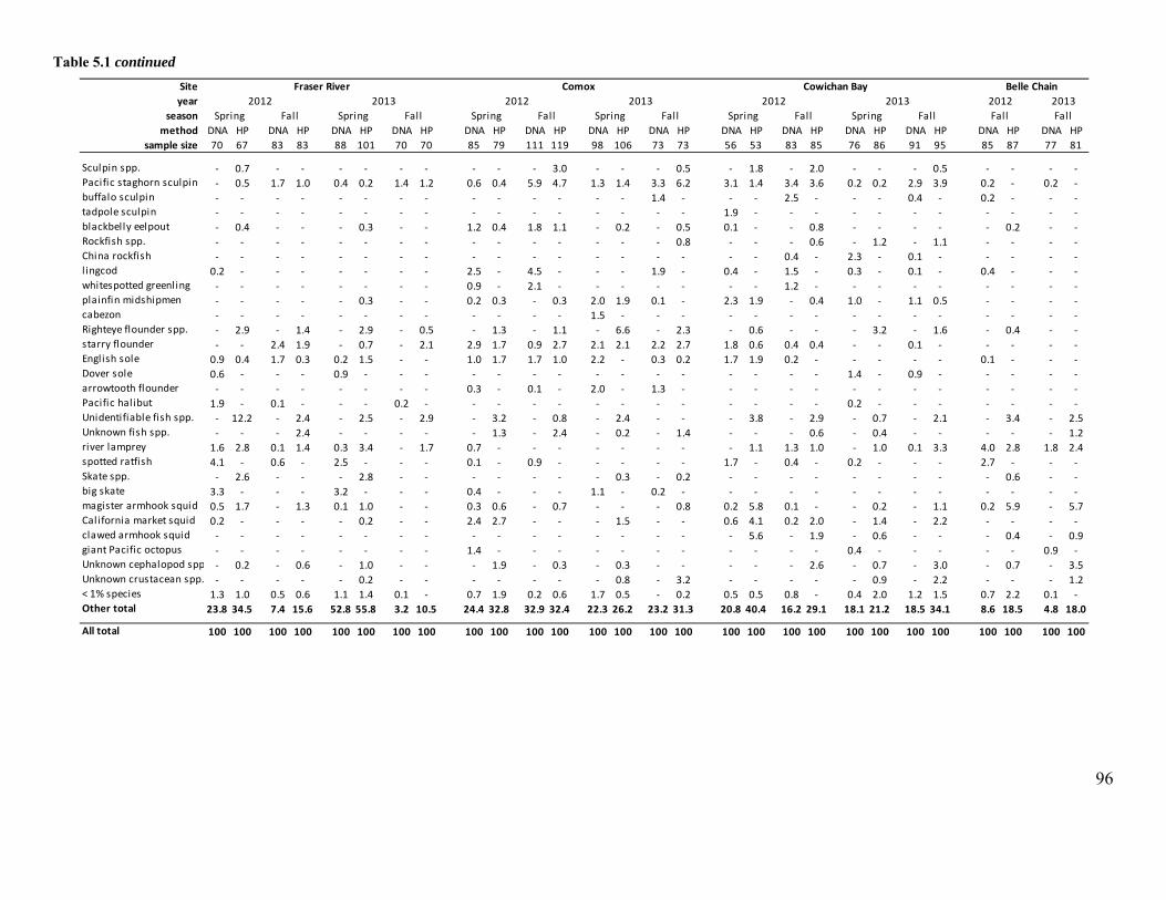
96

Table 5.1 continued

Siteyear

seasonmethod DNA HP DNA HP DNA HP DNA HP DNA HP DNA HP DNA HP DNA HP DNA HP DNA HP DNA HP DNA HP DNA HP DNA HP

sample size 70 67 83 83 88 101 70 70 85 79 111 119 98 106 73 73 56 53 83 85 76 86 91 95 85 87 77 81

Sculpin spp. ‐ 0.7 ‐ ‐ ‐ ‐ ‐ ‐ ‐ ‐ ‐ 3.0 ‐ ‐ ‐ 0.5 ‐ 1.8 ‐ 2.0 ‐ ‐ ‐ 0.5 ‐ ‐ ‐ ‐Pacific staghorn sculpin ‐ 0.5 1.7 1.0 0.4 0.2 1.4 1.2 0.6 0.4 5.9 4.7 1.3 1.4 3.3 6.2 3.1 1.4 3.4 3.6 0.2 0.2 2.9 3.9 0.2 ‐ 0.2 ‐buffalo sculpin ‐ ‐ ‐ ‐ ‐ ‐ ‐ ‐ ‐ ‐ ‐ ‐ ‐ ‐ 1.4 ‐ ‐ ‐ 2.5 ‐ ‐ ‐ 0.4 ‐ 0.2 ‐ ‐ ‐tadpole sculpin ‐ ‐ ‐ ‐ ‐ ‐ ‐ ‐ ‐ ‐ ‐ ‐ ‐ ‐ ‐ ‐ 1.9 ‐ ‐ ‐ ‐ ‐ ‐ ‐ ‐ ‐ ‐ ‐blackbelly eelpout ‐ 0.4 ‐ ‐ ‐ 0.3 ‐ ‐ 1.2 0.4 1.8 1.1 ‐ 0.2 ‐ 0.5 0.1 ‐ ‐ 0.8 ‐ ‐ ‐ ‐ ‐ 0.2 ‐ ‐Rockfish spp. ‐ ‐ ‐ ‐ ‐ ‐ ‐ ‐ ‐ ‐ ‐ ‐ ‐ ‐ ‐ 0.8 ‐ ‐ ‐ 0.6 ‐ 1.2 ‐ 1.1 ‐ ‐ ‐ ‐China rockfish ‐ ‐ ‐ ‐ ‐ ‐ ‐ ‐ ‐ ‐ ‐ ‐ ‐ ‐ ‐ ‐ ‐ ‐ 0.4 ‐ 2.3 ‐ 0.1 ‐ ‐ ‐ ‐ ‐l ingcod 0.2 ‐ ‐ ‐ ‐ ‐ ‐ ‐ 2.5 ‐ 4.5 ‐ ‐ ‐ 1.9 ‐ 0.4 ‐ 1.5 ‐ 0.3 ‐ 0.1 ‐ 0.4 ‐ ‐ ‐whitespotted greenling ‐ ‐ ‐ ‐ ‐ ‐ ‐ ‐ 0.9 ‐ 2.1 ‐ ‐ ‐ ‐ ‐ ‐ ‐ 1.2 ‐ ‐ ‐ ‐ ‐ ‐ ‐ ‐ ‐plainfin midshipmen ‐ ‐ ‐ ‐ ‐ 0.3 ‐ ‐ 0.2 0.3 ‐ 0.3 2.0 1.9 0.1 ‐ 2.3 1.9 ‐ 0.4 1.0 ‐ 1.1 0.5 ‐ ‐ ‐ ‐cabezon ‐ ‐ ‐ ‐ ‐ ‐ ‐ ‐ ‐ ‐ ‐ ‐ 1.5 ‐ ‐ ‐ ‐ ‐ ‐ ‐ ‐ ‐ ‐ ‐ ‐ ‐ ‐ ‐Righteye flounder spp. ‐ 2.9 ‐ 1.4 ‐ 2.9 ‐ 0.5 ‐ 1.3 ‐ 1.1 ‐ 6.6 ‐ 2.3 ‐ 0.6 ‐ ‐ ‐ 3.2 ‐ 1.6 ‐ 0.4 ‐ ‐starry flounder ‐ ‐ 2.4 1.9 ‐ 0.7 ‐ 2.1 2.9 1.7 0.9 2.7 2.1 2.1 2.2 2.7 1.8 0.6 0.4 0.4 ‐ ‐ 0.1 ‐ ‐ ‐ ‐ ‐English sole 0.9 0.4 1.7 0.3 0.2 1.5 ‐ ‐ 1.0 1.7 1.7 1.0 2.2 ‐ 0.3 0.2 1.7 1.9 0.2 ‐ ‐ ‐ ‐ ‐ 0.1 ‐ ‐ ‐Dover sole 0.6 ‐ ‐ ‐ 0.9 ‐ ‐ ‐ ‐ ‐ ‐ ‐ ‐ ‐ ‐ ‐ ‐ ‐ ‐ ‐ 1.4 ‐ 0.9 ‐ ‐ ‐ ‐ ‐arrowtooth flounder ‐ ‐ ‐ ‐ ‐ ‐ ‐ ‐ 0.3 ‐ 0.1 ‐ 2.0 ‐ 1.3 ‐ ‐ ‐ ‐ ‐ ‐ ‐ ‐ ‐ ‐ ‐ ‐ ‐Pacific halibut 1.9 ‐ 0.1 ‐ ‐ ‐ 0.2 ‐ ‐ ‐ ‐ ‐ ‐ ‐ ‐ ‐ ‐ ‐ ‐ ‐ 0.2 ‐ ‐ ‐ ‐ ‐ ‐ ‐Unidentifiable fish spp. ‐ 12.2 ‐ 2.4 ‐ 2.5 ‐ 2.9 ‐ 3.2 ‐ 0.8 ‐ 2.4 ‐ ‐ ‐ 3.8 ‐ 2.9 ‐ 0.7 ‐ 2.1 ‐ 3.4 ‐ 2.5Unknown fish spp. ‐ ‐ ‐ 2.4 ‐ ‐ ‐ ‐ ‐ 1.3 ‐ 2.4 ‐ 0.2 ‐ 1.4 ‐ ‐ ‐ 0.6 ‐ 0.4 ‐ ‐ ‐ ‐ ‐ 1.2river lamprey 1.6 2.8 0.1 1.4 0.3 3.4 ‐ 1.7 0.7 ‐ ‐ ‐ ‐ ‐ ‐ ‐ ‐ 1.1 1.3 1.0 ‐ 1.0 0.1 3.3 4.0 2.8 1.8 2.4spotted ratfish 4.1 ‐ 0.6 ‐ 2.5 ‐ ‐ ‐ 0.1 ‐ 0.9 ‐ ‐ ‐ ‐ ‐ 1.7 ‐ 0.4 ‐ 0.2 ‐ ‐ ‐ 2.7 ‐ ‐ ‐Skate spp. ‐ 2.6 ‐ ‐ ‐ 2.8 ‐ ‐ ‐ ‐ ‐ ‐ ‐ 0.3 ‐ 0.2 ‐ ‐ ‐ ‐ ‐ ‐ ‐ ‐ ‐ 0.6 ‐ ‐big skate 3.3 ‐ ‐ ‐ 3.2 ‐ ‐ ‐ 0.4 ‐ ‐ ‐ 1.1 ‐ 0.2 ‐ ‐ ‐ ‐ ‐ ‐ ‐ ‐ ‐ ‐ ‐ ‐ ‐magister armhook squid 0.5 1.7 ‐ 1.3 0.1 1.0 ‐ ‐ 0.3 0.6 ‐ 0.7 ‐ ‐ ‐ 0.8 0.2 5.8 0.1 ‐ ‐ 0.2 ‐ 1.1 0.2 5.9 ‐ 5.7California market squid 0.2 ‐ ‐ ‐ ‐ 0.2 ‐ ‐ 2.4 2.7 ‐ ‐ ‐ 1.5 ‐ ‐ 0.6 4.1 0.2 2.0 ‐ 1.4 ‐ 2.2 ‐ ‐ ‐ ‐clawed armhook squid ‐ ‐ ‐ ‐ ‐ ‐ ‐ ‐ ‐ ‐ ‐ ‐ ‐ ‐ ‐ ‐ ‐ 5.6 ‐ 1.9 ‐ 0.6 ‐ ‐ ‐ 0.4 ‐ 0.9giant Pacific octopus ‐ ‐ ‐ ‐ ‐ ‐ ‐ ‐ 1.4 ‐ ‐ ‐ ‐ ‐ ‐ ‐ ‐ ‐ ‐ ‐ 0.4 ‐ ‐ ‐ ‐ ‐ 0.9 ‐Unknown cephalopod spp ‐ 0.2 ‐ 0.6 ‐ 1.0 ‐ ‐ ‐ 1.9 ‐ 0.3 ‐ 0.3 ‐ ‐ ‐ ‐ ‐ 2.6 ‐ 0.7 ‐ 3.0 ‐ 0.7 ‐ 3.5Unknown crustacean spp. ‐ ‐ ‐ ‐ ‐ 0.2 ‐ ‐ ‐ ‐ ‐ ‐ ‐ 0.8 ‐ 3.2 ‐ ‐ ‐ ‐ ‐ 0.9 ‐ 2.2 ‐ ‐ ‐ 1.2< 1% species 1.3 1.0 0.5 0.6 1.1 1.4 0.1 ‐ 0.7 1.9 0.2 0.6 1.7 0.5 ‐ 0.2 0.5 0.5 0.8 ‐ 0.4 2.0 1.2 1.5 0.7 2.2 0.1 ‐Other total 23.8 34.5 7.4 15.6 52.8 55.8 3.2 10.5 24.4 32.8 32.9 32.4 22.3 26.2 23.2 31.3 20.8 40.4 16.2 29.1 18.1 21.2 18.5 34.1 8.6 18.5 4.8 18.0

All total 100 100 100 100 100 100 100 100 100 100 100 100 100 100 100 100 100 100 100 100 100 100 100 100 100 100 100 100

Fraser River Comox Cowichan Bay Belle Chain2012 2013 2012 2013 2012 2013

Fall

2012 2013

Spring Fall Spring Fall Spring Fall Spring Fall Spring Fall Spring Fall Fall

97

sampling site is shown by salmon species and life stage for each sampling year in Appendix B:

Comox (Figure B-2; Figure B-3: Figure B-4), Fraser (Figure B-5; Figure B-6; Figure B-7),

Cowichan Bay (Figure B-8; Figure B-9; Figure B-10),and Belle Chain (Figure B-11; Figure

B-12; Figure B-13).

When assigning salmon species DNA percentages to either adult or juvenile life stage, it

was important to note which source of information was used to generate the juvenile/adult

salmon ratio. Of the 756 samples that produced salmon DNA sequences, 419 (55.4%) were

assigned to life stage using the salmon sample SSFO ratio (i.e. the same scat samples contained

identified salmon hardparts). Another 285 (37.7%) samples did not contain salmon hardparts but

were assigned to life stage based on the salmon monthly SSFO ratio because > 3 samples from

the same location/month contained salmon hardparts. Only 52 (6.9%) samples were assigned to

salmon life stage based on the fixed season ratio. Salmon species assignment to life stage was

therefore informed by salmon hardparts data for 93% of samples containing salmon DNA.

Large differences were detected in estuarine harbour seal diet between the 1980s and the

present study when comparing summaries generated using the same method (hardparts SSFO

%), and site type (i.e. estuary sites; Figure 5.3). In the 1980s, harbour seal diet was dominated by

gadoids in both seasons (spring = 47.0%; fall = 46.0%), and salmon comprised a much smaller

portion of the overall diet (spring = 6.0%; fall = 15.7%). This is in contrast to samples collected

during 2012-2013 in which gadoids represented a much reduced portion of harbour seal diet

(spring = 17.5%; fall = 15.1%), and salmonids dominated the diet in the fall (spring = 8.9%, fall

= 43.0%). The herring portion of harbour seal diet was remarkably consistent between both

periods, regardless of the method used to analyze the diet (Figure 5.3).

98

Figure 5.3 Average diets of harbour seals (%) in estuaries during spring and fall based on hardparts SSFO

percentages (1980s and 2012-2013) and DNA metabarcoding diet percentages (2012-2013). Diets were

determined from remains in scats and are grouped into four prey categories (Herring, Gadoids, Salmon,

Other). Total samples included in 2012-2013 estimates were: Spring (n = 473); Fall (n = 540).

99

Figure 5.4 Monthly amounts (%) of juvenile (left) and adult (right) salmon species present in harbour seal

scats collected at haulouts in estuaries (2012-2013). Species were determined using DNA sequencing, and life

stages were determined from a salmon hardparts decision tree analysis. Data represent averages for all

estuary sites and years combined. Sample sizes in each month are indicated in the lower figure margin.

100

Figure 5.5 Percent of adult and juvenile salmon (chum, pink, sockeye, Chinook and coho) contained in harbor

seal scats collected over 4 month periods. Adult salmon were consumed in the fall (Aug – Nov) and juvenile

salmon species were consumed in the spring (Apr – Jul).

DNA metabarcoding diet analysis detected higher levels of salmon in harbour seal diet

than hardparts SSFO analysis for the 2012-2013 samples, increasing the salmon diet percentage

in both seasons. This was particularly apparent in the spring season when the salmon portion of

seal diet doubled by using the DNA-based method (hardparts SSFO = 8.9% salmon; DNA

metabarcoding = 18.0% salmon). Only small differences were observed between methods in the

gadoid and herring portions of harbour seal diet (Figure 5.3).

Life stage specific harbour seal diet percentages for salmon species resulted in clear

seasonal trends in harbour seal salmon predation, pooling samples across years and all 3 estuary

101

sites (Figure 5.4). Low levels of adult salmon predation were observed from April– June and

primarily consisted of Chinook salmon (Oncorhynchus tshawytscha), which peaked at 2.7% of

the overall seal diet in April. Following this period we detected a sequential increase in adult

salmon consumption by harbour seals, with different salmon species peaking in different months.

Adult salmon predation initiated with sockeye (Oncorhynchus nerka) in July, which then peaked

in August and was finished in September. Sockeye predation was followed by pink salmon

(Oncorhynchus gorbuscha) predation, which peaked September and finished in October. Chum

salmon (Oncorhynchus keta) was the last and most important salmon species in harbour seal diet,

beginning in September and peaking in November. Two peaks were observed in adult Chinook

predation, with a small peak in July and a larger peak in September. Adult coho salmon was a

surprisingly small component of the overall seal diet, peaking at 3.4% in October.

Seasonal trends in juvenile salmon predation by seals were less defined, but varied

substantially between salmon species. In contrast to adult salmon predation, coho comprised the

largest component of harbour seal diet in the spring, with peaks of 4.8% in April and 3.9% in

July (Figure 5.4, Figure 5.5). Juvenile Chinook salmon was also an important diet species, with a

combined peak in June and July at 3.9%. Juvenile sockeye and pink salmon predation was

consistent throughout the spring, with no clearly defined peaks in predation at the aggregate

scale. Also in contrast to adult salmon predation, juvenile chum salmon was the least important

of the juvenile diet species for seals (Figure 5.5).

In addition to seasonal variability, we observed marked inter-annual variability in harbour

seal salmon predation between 2012 and 2013 (Figure 5.6). In 2012 for example, adult sockeye

salmon was more important in the seal diet (July = 25.1% and August = 23%) than it was in

2013 when adult sockeye peaked at 16.0% of seal diet. Additionally, the percentage of adult pink

salmon in seal diet was far greater in 2013 than it was in 2012, and appeared to be inversely

related to the percentage of adult Chinook salmon in the seal diet (i.e. the year with high pink

salmon predation had low Chinook predation). Juvenile salmon predation by seals varied

between years as well; coho and Chinook predation for example both peaked in June and July of

2012, but they did not exhibit the same unimodal pattern in 2013. Large differences were also

detected in the percentage of juvenile sockeye consumed between years (Figure 5.6).

102

Figure 5.6 Percentages of salmon (steelhead, sockeye, pink, coho, chum and Chinook) by life stage (juvenile

or adult) in the diets of harbour seals using estuary haulouts in 2012 and 2013. Diets were determined by

month, and sample size indicates the numbers of scats collected each month. Differences between years in

salmon species consumed reflect differences in year class strengths and life histories of the different salmonid

species. Note that steelhead were only detectable in 2012 when the secondary (COI) salmon-specific DNA

marker was used.

103

Figure 5.7 Estimated fork lengths of juvenile salmon (Chinook, coho and sockeye) derived from the few

otoliths recovered in seal scats that were not too eroded to measure. Colors indicate the species of salmon

based on morphological ID, and the letters identify where the seal scat was collected (A = Comox, B =

Cowichan Bay, C = Belle Chain).

Of the 433 salmon otoliths recovered from the harbour seal scats, 363 (84%) were graded

as “poor” due to digestion erosion and could not be used to estimate fish lengths. The remaining

salmon otoliths were paired to represent a minimum number of individual fish, and fork lengths

of juveniles were estimated for 35 salmon otoliths identified to a species (Figure 5.7). As stated,

many juvenile salmon otoltihs were too eroded to measure, and many more were likely

completely digested. However, assuming these 35 otoliths were an unbiased representation of the

juvenile salmon consumed indicates that harbour seals targeted salmon juveniles between 7.8 -

23.4 cm (fork length). During spring (April – July), the seals primarily consumed juvenile

salmon between 5 and 15 cm, and in the fall (August – November) seals targeted juveniles

between 15 and 25 cm. The majority of identifiable otoliths were Chinook salmon, but coho and

sockeye otoliths were also identified.

Several prey species in the “other” category are worth noting because they contributed

significantly (> 2%) to overall harbour seal diet in one of the two seasons (all estuaries and years

104

combined). Three-spined stickleback (Gasterosteus aculeatus) comprised 7.5% of overall seal

diet in the spring season and eulachon (Thaleichthys pacificus) comprised 5.5% of the spring diet

as well. In the fall season, shiner perch (Cymatogaster aggregata) made up 5.3% of overall seal

diet and Pacific staghorn sculpin (Leptocottus armatus) contributed 3.5%.

5.5 Discussion

We applied DNA metabarcoding diet analysis and morphological prey hardparts analysis

to 1,240 harbour seal scat samples collected from haulout sites in the Strait of Georgia, Canada.

We then merged data generated from both methods to estimate the species and life stages of

salmon consumed by seals to facilitate predator-prey modeling. The vast majority of our samples

containing salmon were assigned to a life stage (juvenile of adult) based on the co-occurrence of

salmon bones in the sample or collection month. Comparisons between our study and historic

harbour seal diet indicate that adult salmon consumption by harbour seals increased substantially

since the 1980s―and our methods comparison suggests that juvenile salmon consumed by seals

may be particularly underestimated using only hardparts techniques. The combined hardparts and

DNA data enabled us to identify clear seasonal trends in seal consumption of salmon species that

are specific to salmon life stage.

5.5.1 Diet analysis methods

Pinniped diet analysis using DNA metabarcoding is a relatively new technique that offers

several advantages over previous molecular diet analysis tools (Deagle et al. 2009; Clare 2014;

Symondson and Harwood 2014). Prior studies have mostly relied on species or group-specific

primer sets and gel-based methods to identify pinniped prey; often limiting DNA identification

to only a subset of prey taxa and requiring a mathematical model to convert prey occurrences

into diet percentages (Purcell et al. 2004; Parsons et al. 2005; Tollit et al. 2009). Quantitative

real-time PCR (qPCR) can be used with taxon specific primers for prey quantification from scat

DNA, but the global diet is difficult and costly to calculate using many different species specific

primers (Matejusová et al. 2008; Bowles et al. 2011; Matejusová et al. 2012). Conversely, DNA

metabarcoding diet analysis employs universal primers to simultaneously amplify many (if not

all) prey species, relying on high-throughput DNA amplicon sequencing to identify and quantify

105

prey. Furthermore, amplicons of many individual samples can now be sequenced simultaneously

and differentiated using bioinformatic techniques, dramatically reducing the per sample cost of

DNA diet analysis.

Proportional estimates of predator global diet are important for calculating estimates of

prey consumption such as the numbers of individual fish eaten by a pinniped population (Olesiuk

1993; Winship and Trites 2003; Howard et al. 2013). In our study, prey DNA sequence

percentages were averaged from large numbers of individual seal scat samples to calculate

population level diet percentages. This approach generally assumes a quantitative relationship

between DNA sequence read proportions from seal scat samples, and the overall biomass

proportions of prey consumed by the seal population. Captive feeding studies with pinnipeds and

other marine predators have indicated that the relationship between prey DNA sequence

percentage and prey biomass is not linear, but most studies have ultimately concluded that DNA

metabarcoding can be treated as a semi-quantitative tool (Deagle et al. 2010; Pompanon et al.

2012; Thomas et al. 2014). In addition, studies such as ours which aim to characterize the diets

of consumer populations appear to be less influenced by quantification biases than studies

focused on the diets of individual animals (Thomas et al. unpubl. data). The accuracy of our

harbour seal DNA diet estimates could likely be improved by creating a complete harbour seal

prey library of tissue mix standards and applying species-specific correction factors (Thomas et

al. unpubl. data).

Merging harbour seal DNA diet data with prey hardparts information enabled us to

estimate the proportions of adult and juvenile salmon consumed by harbour seals, in addition to

identifying the salmon species and percentage of the overall diet. To our knowledge, these are

the first such estimates from pinniped scat samples. The method we created to assign salmon

species to life stage relied first on the co-occurrence of salmon bones in the individual scat, then

on occurrences of salmon bones in scats collected at the same site/month, and as a last resort,

assignment was made based on a fixed seasonal ratio of adults to juvenile salmon. This design

prioritizes the best available information to assign the salmon life stages.

Three pieces of evidence support the appropriateness of our method for assigning a life

stage to salmon species in harbour seal diet. First, 93% of samples containing salmon DNA were

assigned to life stage based on salmon bone occurrences in the same scat sample or in scat

106

samples collected in the same location and month. Only 7% of salmon samples relied on the

fixed season ratio to assign salmon life stage. Second, the fixed season ratio (assuming juvenile

salmon consumption in spring, and adult salmon consumption in fall) is generally supported by

the occurrences of adult and juvenile salmon bones in those seasons (Figure B-2). The only

major exception to this assumption was the occurrence of adult sockeye salmon in July in the

Fraser River estuary; adults of all other species were primarily consumed in what we defined as

the fall season. The final piece of evidence supporting our salmon life stage assignment protocol

is the fact that the resulting estimates of harbour seal diet demonstrate a clear functional response

by seals to the seasonal abundances of salmon, which corresponds well to the movements of

adult and juvenile salmonids in the Strait of Georgia (Quinn 2005).

Our study focused on the diet of a piscivorous marine mammal. However, the framework

we used to merge DNA and hardparts data could be applied to any study system in which it is

possible to recover both DNA and hard prey structures from diet samples. The diets of arthropod

predators for example could potentially be refined to prey life stages, if exoskeleton fragments in

predator scats could be identified to arthropod life stage (Clare et al. 2009; Clare et al. 2014).

Similarly, the age classes of small mammals consumed by terrestrial predators can be estimated

based on the co-occurrence of DNA in predator feces and animal bones for which age-bone size

relationships have been established (Longland and Jenkins 1987; Shehzad et al. 2012). Because

prey life stage has such a large influence on the ecosystem dynamics introduced by predation,

there is a need for trophic ecologists to produce predator diet data that is both species and life

stage specific.

5.5.2 Food habits of harbour seals in estuaries

In addition to supporting methodological advancement, our analysis also provides new

insight into the foraging behaviour of harbour seals in the Strait of Georgia. The observed

increase in harbour-seal salmon consumption since the 1980s was unexpected, indicating a

nearly threefold increase in fall salmon consumption based on directly comparable analyses. This

increase in salmon consumption also appears to have corresponded with a large decrease in the

importance of gadoids in harbour seal diet in both seasons. DNA analysis of the 2012-2013

samples confirmed these temporal changes in harbour seal diet.

107

A potential but improbable explanation for the observed increase in fall salmon

consumption is that differences in seal diet could be due to sampling differences between the two

periods. The 1980s study sampled a greater number of estuarine harbour seal haulout sites.

However, both studies used sampling sites representing the same major geographical areas. For

example, the Comox and Cowichan Bay haulout sites contributed largely to both the 1980s study

and ours, and the Fraser River region was also represented in both studies. While we chose a

more geographically focused sampling design to detect localized seasonal trends, our sampling

sites were chosen specifically to be comparable with the estuarine sites used in Olesiuk et al.

(1990).

The more plausible explanation for the increase in harbour seal salmon consumption is

that their primary prey in the 1980s (gadoids―mostly Pacific hake) decreased substantially in

abundance since the previous seal diet study. A 1998 survey of Pacific hake in the Strait of

Georgia placed the hake biomass at less than half (i.e. 42%) of the biomass observed in a

comparable hake survey in 1981 (Kieser et al. 1999). If this downward trend in hake biomass

continued, harbour seals in our study region would have likely switched to other prey resources

(e.g. adult salmon) that were more readily available (Stephens and Krebs 1986). Furthermore, the

number of harbour seals in the Strait of Georgia more than doubled since the previous diet study,

indicating that different prey resources were likely exploited by harbour seals to sustain the

increased population (Olesiuk 2009). By contrast, the percentage of Pacific herring in harbour

seal diet was remarkably consistent between time periods, and was also consistent between the

two diet analysis techniques.

When the DNA-based method was applied to the same set of scat samples used for

morphological analyses, the percentage of salmon in harbour seal diet increased in both seasons.

The proportional increase in salmon consumption was particularly apparent in the spring season,

when the diet percentage of salmon doubled using DNA metabarcoding. This could indicate a

taxonomic bias in DNA amplification or sequencing that causes salmon to be overestimated

relative to other species; although an evaluation of the methods did not suggest a biased

representation of salmonids (Thomas et al. in prep.). A more likely explanation for the observed

methodological differences is that some salmon prey hardparts were completely digested, or

salmon soft tissue was ingested without ingesting bones (e.g. “belly biting”) (Cottrell et al. 1996;

108

Hauser et al. 2008). The proportional increase in the spring season when seals primarily eat

juvenile salmon, combined with the large number of highly eroded juvenile salmon bones in

scats, suggests that juvenile salmon consumption by pinnipeds may be highly underestimated

using traditional hardparts analysis. It appears likely from our analysis that many of the juvenile

salmon eaten by seals are completely digested and therefore not detectable using hardparts

techniques.

The combination of a near threefold increase in fall salmon consumption by seals and a

doubling of the seal population since the 1980s appears to be cause for concern―indicating that

seals are likely impacting salmon stocks (Olesiuk 2009; Scordino 2010). However, the adult

salmon species primarily consumed by harbour seals in the Strait of Georgia estuaries were not

the species currently of conservation concern (Irvine et al. 2009; Welch et al. 2011). Seals

mostly targeted adult chum salmon in the fall, with pinks and sockeye also contributing

significantly to seal diet in alternate years. The populations of these species were stable overall

or increased in the region, and appeared to be thriving despite increased predation pressure from

seals (Irvine et al. 2009). Also interesting was the inverse interanual relationship in the

percentage of adult Chinook salmon in seal diet relative to pink salmon in seal diet. Regional

pink salmon runs are large in odd-numbered years and low in even-numbered years―and there

may be a predation masking effect occurring, whereby the presence of many pink salmon in

September reduces seal predation pressure on adult Chinook salmon (Holling 1966; Evans

2013). These results emphasize the importance of knowing the particular species consumed by

predators when assessing their potential impacts on prey populations.

While the species composition of adult salmon eaten by harbour seals does not raise

concern for salmon stocks, the composition of juvenile salmon species in seal diet displayed the

opposite trend. Harbour seals consumed higher percentages of juvenile coho, Chinook, and

sockeye salmon in the Strait of Georgia, despite the exceeding abundance of juvenile chum

salmon in the region (Beamish et al. 2012). This implies that harbour seals may be selective (i.e.

consuming disproportionately to fish abundance) of the juvenile salmon species they choose to

pursue (Manly et al. 1993). Positive selection often occurs when less abundant prey species are

more profitable (e.g. contains higher energy density, or requires less energy to capture) than the

more abundant prey species (Stephens and Krebs 1986; Tollit et al. 1997a). Interestingly, all

109

three of the juvenile salmon species consumed by seals in relatively high proportion (coho,

Chinook, and sockeye) consist of stocks that undergo seaward migration at age > 1 y. In contrast,

the juvenile salmon species eaten by the seals in smaller proportions (pink and chum) all of out-

migrate at age < 1 y (Randall et al. 1987; Quinn 2005). This implies that harbour seals may be

selecting for older, larger salmon smolts that are more profitable to pursue than chum and pink

fry. These older juvenile salmonids may also better fit the prey search image of harbour seals,

both in terms of size and coloration (Tollit et al. 1997a).

Although the percentages of juvenile salmon species in harbour seal diets were relatively

small (generally < 5% per species), such percentages can be significant when converted to

numbers of fish —particularly when a large number of predators consume many small-bodied

prey species. For example, ~40,000 adult harbour seals (the current population in the Strait of

Georgia) consuming an average of 2 kg per day would eat ~6 million coho smolts in one month,

assuming the average hatchery coho smolt weighs ~ 20g, and seal diet consists of 5% juvenile

coho (Olesiuk 1993; Olesiuk 2009; Howard et al. 2013). Considerably more smolts could be

consumed if the smolts were smaller (e.g., wild coho smolts).

This rough estimate of the numbers of coho smolts consumed also assumes that all seals

in the Strait consume juvenile salmon at the same average rate, which is unlikely to be true for

the many seals that inhabit non-estuary haulout sties. In addition, measured salmon predation is

likely to be substantially lower at non-estuary harbour seal haulouts sites. However, it is worth

noting that the single highest percentage of juvenile Chinook salmon in seal diet for any stratum

in our study was from the Belle Chain collection site (a non-estuary harbour seal haulout) (Table

1). In-depth modeling will be required to produce robust estimates of harbour seal consumption

of juvenile and adult salmon species in the Strait of Georgia based on the dietary data we

generated.

5.5.3 Accuracy of juvenile salmon percentage of seal diet

Given that harbour seals have the potential to largely impact juvenile salmonids when

juveniles comprise a relatively low percentage of the overall seal diet, it is important to produce

accurate seal diet estimates for those species. We have focused on using DNA sequence counts

to infer the relative biomasses of prey consumed by seals — an approach that now has well

110

Figure 5.8 Comparison of three different methods used to calculate harbour seal population diet percentages

from the same set of scat samples in two different seasons: Spring (when harbour seals primary eat juvenile

salmon); Fall (when harbour seals mostly eat adult salmon). The methods applied were, a) Split Sample

Frequency of Occurrence of prey hardparts (blue), b) Split Sample Frequency of Occurrence of prey DNA

(yellow), c) DNA sequence percentages resulting from DNA metabarcoding (red). Data are from Comox,

2012.

111

documented biases. To truly understand the numerical accuracy of seal DNA metabarcoding diet

estimates (at the individual or population level) would require extensive feeding trials that are

beyond the scope of this work, and are likely infeasible due to the number of factors that would

need to be evaluated. Rather than attempting to quantify the accuracy of specific estimates, we

can evaluate whether DNA sequence percentages are likely to produce diet estimates that are

more or less accurate compared to the other available methods.

To circumvent the biases with DNA sequence counts, trophic ecologists often remove the

quantitative information from DNA metabarcoding studies and present a presence/absence based

index such as frequency of occurrence. This is similar to the way that scat hardparts data are

often treated, and the way we presented them here (Split Sample Frequency of Occurrence).

Using scats collected from one haulout site, we compared diet percentages calculated three ways

using the same set of samples: 1) diet % based on morphological identification of prey bones and

Split Sample Frequency of Occurrence (i.e. Hardparts SSFO), 2) removing the quantitative DNA

sequence information and treating each species occurrence equally ( i.e. DNA SSFO), and 3)

retaining the quantitative information from sequence counts and assuming a relationship between

DNA sequences % and prey biomass (i.e. DNA sequences %) . Comparing these three methods

with previous studies provides insights into which technique is most likely to produce the best

estimate of juvenile salmon in harbour seal diet (Figure 5.8).

If DNA sequence percentages produce consistently biased estimates of harbour seal

salmon consumption, we would expect that DNA sequences % would be largely different from

the other two occurrence-based estimates. This was however not the case. When seals were

eating primarily adult salmon (fall), the “All salmonids” combined percentages of the diet were

quite similar between the three methods we compared (Figure 5.8). However, in the spring

months when seals were mostly eating juvenile salmon, both DNA techniques produced higher

diet estimates for salmon (Figure 5.8). As stated previously, this is most likely due to the

complete digestion of juvenile salmon bones which leads to lower salmon detection when

hardparts techniques are used. What was unexpected was the large increase in spring salmon

percentage when prey DNA sequences were treated as occurrences (SSFO) as compared to DNA

sequences %. This suggests that many seal scat samples in the spring contained salmon DNA in

small quantities, which were then overestimated by treating DNA detections as occurrence data.

112

Interestingly, in many cases the use of DNA sequence percentages produced estimates that were

more similar to hardparts SSFO than DNA SSFO — despite the two DNA estimates being

derived from the exact same sequence data.

Based on this evidence, and the fact that prey DNA sequence percentages generally

increase with prey biomass (Chapter 4), we conclude that DNA sequences % is likely the most

accurate method for estimating the percentages of juvenile salmon consumed by harbour seals.

Where hardparts methods appear to underestimate juvenile salmon predation and DNA SSFO

likely overestimates the importance of juvenile salmon, DNA sequence percentages produce a

conservative and realistic estimate of diet. Despite the factors that are known to influence

sequence counts in DNA metabarcoding studies, our findings suggest that using DNA sequence

percentages is currently superior to methods that treat all prey detections as occurrences of equal

weight. Therefore, we believe that the data set presented here currently provides the most

accurate estimate available for the proportion of juvenile salmon species in the diets of harbour

seals in the Strait of Georgia.

5.6 Conclusion

Demand is increasing for better descriptions of predator diets, including information

about the species and life stage of prey, the proportional biomass consumed, as well as the

specific sub-population of prey impacted by the predators. Trophic ecologists are responding to

this demand by exploring alternative methods to analyze diets (such as merging data from

multiple dietary methods to create consensus predator diet data) which provide information that

cannot be produced by traditional techniques. We demonstrated how DNA metabarcoding diet

analysis and prey hardparts analysis can be merged to estimate the species, life stage, and

relative proportion of salmon consumed by harbour seals. The general approach we outlined for

doing so can be used in a variety of study systems to derive better information about predator

diets. The combination data product we generated enabled us to identify seasonal trends in

harbour seal predation on different life stages of salmon, in addition to allowing us to document

a major shift in harbour seal foraging behaviour since the 1980s. Ideally, this approach can be

integrated into an ongoing marine predator diet survey, recognizing that animal diets can change

continuously in response to changes in prey abundance and intraspecific competition.

113

Chapter 6: General conclusion

The primary objective of my thesis research was to generate harbour seal diet information

that could be used to estimate the numbers of juvenile salmon consumed by seals in the Strait of

Georgia. However, it became apparent upon starting the project that the existing pinniped diet

analysis methodologies were insufficient to produce those estimates because they could not

provide the necessary detail about prey consumed by seals. A new diet analysis technique was

needed to generate the desired harbour seal consumption estimates for salmon. The emerging

diet analysis techniques using DNA metabarcoding offered tremendous potential to quantify the

species proportions of prey consumed by harbour seals, and when combined with traditional

hardparts techniques could be used to estimate both the species and life stages of salmon eaten

by seals in the Strait. I therefore sought to develop a DNA metabarcoding diet analysis tool for

Pacific harbour seals specifically, in addition to evaluating the quantitative potential of the

methodology as it applies to the study of any animal diet.

6.1 Summary of research and findings

Chapter 2 explored the factors that could potentially influence sequence read counts in

DNA metabarcoding diet studies that could bias estimates of species proportional biomass based

on DNA sequence reads. Numerous factors were evaluated in the study, ranging from bias

introduced by short primer tags to biases generated during bioinformatic filtering. The general

conclusion from this work was that virtually every factor we evaluated exhibited some biasing

influence on the species DNA sequence read counts. Taxonomic bias, or the preferential

amplification and sequencing of certain prey DNA sequences over other prey species, was

particularly influential. Although it was confirmed that scats of predators fed a similar diet

produce similar DNA sequence percentages, the results of the study suggest that it is unwise for

researchers to assume a direct relationship between prey biomass % and scat DNA sequences %.

Furthermore, the influence of various biasing factors in DNA metabarcoding diet studies is

highly related to the particular study system. For example, studies in which priming regions are

not highly conserved will be more subject to taxonomic biases in amplification, and other biases

such as those produced by primer tags are sequence specific. Therefore it should be considered

best practice for researchers to evaluate the range of potential biases inherent to their study

114

system when undertaking any new DNA metabarcoding diet study. This is especially important

when DNA sequence counts are used as a proxy for prey biomass; although even basic frequency

of occurrence metrics can be affected when biases are extreme.

The fact that it is possible to achieve consistent prey DNA sequence percentages from the

scats of predators fed a similar diet was intriguing. It implies that it may be possible to correct

for the biases detected in Chapter 2 using numerical correction factors, if the sources of bias are

consistent and quantifiable. Given the number of biases identified in Chapter 2, it appeared

unrealistic to account for each source of bias individually. I therefore sought to find some way of

accounting for as many sources of bias as possible with a minimal number of corrections.

Preparation of control materials (in this case prey tissue mixes) sequenced alongside scat

samples seemed a promising method that could account for many sources of bias simultaneously.

Thus in Chapter 3 I used a prey tissue mix matching captive harbour seal diet and scat samples to

create prey-specific numerical correction factors that account for methodological biases and

template copy number bias. I also evaluated which characteristics of the prey species could

potentially be used to account for biases introduced by differential prey digestion (inferred by the

difference between scat DNA % and tissue mix DNA %).

I found that the majority of bias in the study system could be accounted for using the prey

tissue mix, implying that the primary source of bias was either due to prey differences in

template DNA copy number or preferential PCR amplification and sequencing. The degree of

species-specific bias detected in the tissue mixture was well predicted by the prey fish red

muscle %, further supporting the idea that differential mtDNA density (i.e. template copy

number) is the primary source of bias in the system. Differential prey digestion was the lesser

source of bias, and an analysis of prey composition indicated that a correction based on prey

lipid content could entirely account for prey digestion bias in pinniped diet studies. While these

findings were exciting scientifically, the difficulty encountered was in applying these findings to

samples of unknown composition (such as field studies of wild harbour seals). It is not possible

to design prey tissue mixes that perfectly match the diets of wild seals (because the diet is

unknown), and variability in fish lipid content both seasonally and geographically inhibits

digestion bias correction. For numerical correction factors to be employed in field studies of wild

harbour seals, an alternative approach would be required.

115

The most feasible alternative approach for tissue based correction that I could imagine

was the generation of a 50/50 Tissue Correction Factor prey library (see Chapter 4). Under this

scenario the species-specific bias for any particular prey would be quantified relative to a control

species that is held constant in all mixtures of the prey library. A mathematical formula can then

be used to calculate a numerical correction for any species in the prey library, and those

corrections can be applied to sequence counts generated from seal scat samples of unknown

composition. My experiments in Chapter 4 supported the notion that DNA sequence count biases

are indeed specific to the particular prey species, varying little between individual fishes or

between replicate tissue mix samples. One unexpected result in Chapter 4 was the influence of

the input mass percentage on the degree of bias (and by extension the correction factor). Species

present in low proportion were overestimated and species in high proportion were

underestimated. This result has implications for all kinds of studies aiming to quantify DNA or

organisms using read counts from high-throughput amplicon sequencing; although proportional

bias appeared less influential for more complex species mixtures.

Application of 50/50 tissue correction factors greatly improved the proportional estimates

of multi-species mixtures based on DNA sequence read percentages. However, proportional

estimates for individual scat samples were much more influenced by correction factors than

population diet summaries (i.e. proportional averages generated from many scat samples

combined). Predator consumption estimates typically rely on population diet averages, and the

accuracy of diet percentages for any individual sample is less important for answering questions

of population prey consumption. This begs the question, when is it actually important to achieve

highly accurate individual sample diet estimates?

My rationale for pursuing accurate proportional estimates for individual samples was that

consistent species biases (such as those I have demonstrated for harbour seal prey) have the

potential to largely affect even population level summaries. This would be particularly true if the

population diet was comprised few species (low species diversity) that have strong biases, or

biases in opposing directions. In this case, population summaries could be strongly influenced by

individual species biases and correction factors are likely necessary. However, when diet

diversity is high, species-specific biases likely have much less influence on population diet

summaries. Ultimately the question of whether or not to pursue correction factors should be

116

properly evaluated using an in silico modeling exercise wherein variability of the population diet

estimate is quantified under alternative diet diversity and bias magnitude scenarios.

At this point in my research I was posed with a dilemma. Should I continue to develop

these correction factors for application to my field collected harbour seal scat samples, or should

I move forward without corrections for the population diet summaries? Furthermore, if

corrections were not applied, should I treat the DNA sequence data as frequency of occurrence

(i.e. presence or absence of diet species) or should I continue to use the species sequence count

percentages as a proxy for diet biomass percentage? The answer to the first question was simply

a matter of time and money. To create an exhaustive prey library for harbour seals would be a

large undertaking requiring the collection of dozens of prey specimens (many of which are

difficult to acquire) and many hours of grinding fish and creating tissue mixtures. While I

continue to believe that this may be a worthwhile endeavor, it should first be shown

mathematically that the increase in population estimate accuracy is worth the months of effort

that would be required.

The question of whether or not to remove the “quantitative” information from the prey

DNA sequence counts is a continued matter of debate among molecular trophic ecologists.

Ultimately either diet metric used (frequency of occurrence or DNA sequence %) will be

converted into a proportional diet estimate and used to quantify prey consumption. Therefore, the

real question is, can more accurate diet estimates be achieved by converting prey occurrences to

percentages (e.g. Split Sample Frequency of Occurrence) or by using DNA sequence

percentages?

I chose to use uncorrected DNA sequence percentage as a proxy for prey biomass

percentage for two reasons. First, my prey tissue mixing experiments indicated that an increase

in species proportional biomass does increase the number of prey DNA sequences, even though

the relationship is not perfectly linear and the intercept varies by species. My results support the

idea that DNA sequence counts are semi-quantitative regardless of the known biases. My second

reason for using uncorrected DNA sequence percentages is that frequency of occurrence metrics

are highly sensitive to contamination, even very low level contamination of species DNA in a

sample. One DNA sequence from a contaminating species in a sample is equal to multiple

thousands of DNA sequences from a true diet species in the sample, if Split Sample Frequency

117

of Occurrence is used to create the diet summary. Given that low level contamination has been

demonstrated between multiplexed samples and between Next-gen sequencing runs, the use of

DNA sequence percentages is arguably the more conservative approach to achieve a proportional

diet summary.

Throughout my PhD research, I have attempted to devise novel solutions to difficult

methodological problems, and believe that I achieved moderate success with the use of tissue-

based and/or lipid-based correction factors for DNA sequence counts. However, I think that

Chapter 5 reflects my larger contribution by combining scat DNA sequence percentages with

prey bones to estimate the species and life stages of salmon consumed by seals. A dataset

providing age-specific proportional estimates of the salmon species consumed by seals

represents a significant step forward for the field. In addition, the knowledge that harbour seals

in the Strait of Georgia appear to target adult salmon of low conservation concern and juvenile

salmon of high conservation concern, is highly valuable information for regional fisheries

managers. Moving forward, I will be working with a fisheries modeler to create estimates of

harbour seal salmon consumption from the dataset generated in Chapter 5.

6.2 Applying DNA metabarcoding diet analysis in other study systems

The process of applying the methods outlined in my thesis to other study systems or

predator species would follow a similar procedure to that used in any new DNA metabarcoding

study. The first step is to identify the potential range of food species taxonomic groups, using the

results of previous diet studies and animal observations to narrow down the list of potential food

species. Once the taxonomic list has been established, the next step is to find genetic barcoding

markers (e.g. COI, 16S, 18s) that contain suitable priming regions which are highly conserved

for all potential prey, and also flank a short (< 300 bp) variable marker region useful for species

identification. Once the ideal metabarcoding marker has been identified, primers should be tested

and validated using the extracted DNA of known food species.

At this stage in the project development, it is likely worthwhile to evaluate any potential

taxonomic biases in prey species amplification, if the researchers intend to use DNA sequence

counts to inform consumer diet proportions. A 50/50 tissue mixture prey library such as the one

described in Chapter 4 is one method that could be used to evaluate taxon-specific biases,

118

informing researchers if they should expect large differences in amplicon DNA sequences from

the same mass proportions of different prey species. Depending on the research question and the

importance of accurately determining the proportions of prey in individual scats, researchers

could proceed simply knowing where to expect taxonomic bias in DNA sequence counts. If it is

determined that a high degree of accuracy is needed at the individual scat level, correction

factors could be explored similar to the approach we outlined in Chapters 3 and 4.

The final project development steps are to generate a prey library of species sequences

for the DNA metabarcoding marker, and to create a bioinformatic pipeline for processing

samples of unknown composition. In my thesis work, I benefited from the DNA barcoding

efforts of many other researchers who were actively producing 16S DNA sequences for the

various fishes of the North Pacific. Marker DNA sequences from voucher specimens are often

made publically available in NCBI GenBank and the Barcode of Life Database (BoLD)

(Ratnasingham and Hebert 2007; Benson et al. 2012). For study systems that are less well

described, researchers may need to produce DNA sequence data for their taxonomic groups of

interest following the standardized protocols for producing DNA barcode data (Ratnasingham

and Hebert 2007). Lastly, a bioinformatic pipeline must be established to demultiplex the DNA

sequences of multiple samples sequenced simultaneously (if samples are multiplexed), and to

identify the taxonomy of the DNA sequences assigned to diet samples. Population diet

summaries can then be produced for the consumer of interest by combining the resulting diet

data from multiple individual samples collected in the same region or time period.

6.3 Future directions

The field of DNA metabarcoding diet analysis continues to grow rapidly as the cost of

next-gen DNA sequencing drops, and more user-friendly or established bioinformatic pipelines

become available to ecologists. It is reasonable to expect that this type of diet analysis will soon

become an established methodology widely used by ecologists, similar to stable isotope analysis

(for example). To mitigate the now well-characterized biases inherent to amplicon sequencing, it

appears the field is attempting to move away from targeted PCR enrichment to other approaches

that may produce less biased results. Simple shotgun sequencing of all DNA present in a sample

is one way to reduce PCR enrichment bias, in addition to other alternatives such as filter-based

119

mitochondrial enrichment. Straight DNA sequencing unfortunately produces a huge amount of

sequence data that is not useful for answering the question of interest, and substantially increases

the cost of analysis. I suspect that any new approach will ultimately be shown to introduce

certain biases when researchers fully scrutinize the process. However such continued efforts to

reduce methodological bias are valuable and may ultimately identify a superior method to

amplicon sequencing.

One thing that I think has been lacking in the captive feeding study literature is an

evaluation of alternative methods (quantitative DNA analysis vs hard-parts analysis), where the

diets of the predators are randomized and contain a variety of different species; thereby

simulating a population of scat samples more similar to what is found in studies of wild animals.

Furthermore, these captive studies should be blind trials such that the analyst (morphological

taxonomist or DNA bioinformatician) does not know what the captive predator species has been

fed. With that type of study design it would be possible to empirically measure the accuracy of

population diet summaries generated using alternative techniques and determine which is

ultimately superior — both in terms of biomass estimates and taxonomic resolution/accuracy.

That, combined with an in silico analysis of species-specific biases in DNA metabarcoding

studies (as previously mentioned) would be useful for guiding future DNA diet studies involving

pinnipeds.

Until those additional methodological studies have been conducted, I believe that the

approach outlined in Chapter 5 is currently the best available method for characterizing the diets

of seals and sea lions. My assessment is based on the relative data quality provided by the

technique with respect to taxonomic resolution, quantitative capability, prey age-class

specificity, and per-sample cost of processing. While I do not recommend the abandonment of

traditional diet analysis methods, I do suggest that pinniped ecologists consider transitioning

their ongoing diet studies to a hybrid DNA/hard-parts approach such as the one we used in

Chapter 5. Time will ultimately determine which pinniped diet analysis method is best, and I

look forward to observing the future evolution of DNA metabarcoding in the field of trophic

ecology.

120

References

Acinas, S.G., R. Sarma-Rupavtarm, V. Klepac-Ceraj, and M.F. Polz. 2005. PCR-induced sequence artifacts and bias: Insights from comparison of two 16S rRNA clone libraries constructed from the same sample. Applied and Environmental Microbiology 71:8966-8969.

Altschul, S.F., W. Gish, W. Miller, E.W. Myers, and D.J. Lipman. 1990. Basic local alignment search tool. Journal of Molecular Biology 215:403-410.

Amend, A.S., K.A. Seifert, and T.D. Bruns. 2010. Quantifying microbial communities with 454 pyrosequencing: does read abundance count? Molecular Ecology 19:5555-5565.

Andersen, K., K.L. Bird, M. Rasmussen, J. Haile, H. Breuning-Madsen, K.H. KjÆR, L. Orlando, M.T.P. Gilbert, and E. Willerslev. 2012. Meta-barcoding of ‘dirt’ DNA from soil reflects vertebrate biodiversity. Molecular Ecology 21:1966-1979.

Angly, F.E., P.G. Dennis, A. Skarshewski, I. Vanwonterghem, P. Hugenholtz, and G.W. Tyson. 2014. CopyRighter: a rapid tool for improving the accuracy of microbial community profiles through lineage-specific gene copy number correction. Microbiome 2:1-13.

Anonymous. 1999. Protocol for the Scientific Evaluation of Proposals to Cull Marine Mammals. In Report of the Scientific Advisory Committee of the Marine Mammals Action Plan. United Nations Enironmental Program. Rome, Italy. 25 pp.

Beamish, R., C. Neville, R. Sweeting, and K. Lange. 2012. The synchronous failure of juvenile Pacific salmon and herring production in the Strait of Georgia in 2007 and the poor return of sockeye salmon to the Fraser River in 2009. Marine and Coastal Fisheries 4:403-414.

Beltran, R.S., M.C. Sadou, R. Condit, S.H. Peterson, C. Reichmuth, and D.P. Costa. 2015. Fine-scale whisker growth measurements can reveal temporal foraging patterns from stable isotope signatures. Marine Ecology Progress Series 523:243-253.

Ben-David, M., and E.A. Flaherty. 2012. Stable isotopes in mammalian research: a beginner's guide. Journal of Mammalogy 93:312-328.

Benson, D.A., M. Cavanaugh, K. Clark, I. Karsch-Mizrachi, D.J. Lipman, J. Ostell, and E.W. Sayers. 2012. GenBank. Nucleic Acids Research 28:15-18.

Berry, D., K. Ben Mahfoudh, M. Wagner, and A. Loy. 2011. Barcoded primers used in multiplex amplicon pyrosequencing bias amplification. Applied and Environmental Microbiology 77:7846-9.

Bik, H.M., D.L. Porazinska, S. Creer, J.G. Caporaso, R. Knight, and W.K. Thomas. 2012. Sequencing our way towards understanding global eukaryotic biodiversity. Trends in Ecology & Evolution 27:233-243.

Bowen, W., and S. Iverson. 2013. Methods of estimating marine mammal diets: A review of validation experiments and sources of bias and uncertainty. Marine Mammal Science 29:719-754.

Bowen, W.D., and D. Lidgard. 2013. Marine mammal culling programs: review of effects on predator and prey populations. Mammal Review 43:207-220.

Bowles, E., P.M. Schulte, D.J. Tollit, B.E. Deagle, and A.W. Trites. 2011. Proportion of prey consumed can be determined from faecal DNA using real-time PCR. Molecular Ecology Resources 11:530-40.

Brown, D.S., S.N. Jarman, and W.O.C. Symondson. 2012. Pyrosequencing of prey DNA in reptile faeces: analysis of earthworm consumption by slow worms. Molecular Ecology Resources 12:259-266.

Budge, S.M., S.J. Iverson, and H.N. Koopman. 2006. Studying trophic ecology in marine ecosystems using fatty acids: a primer on analysis and interpretation. Marine Mammal Science 22:759-801.

Buée, M., M. Reich, C. Murat, E. Morin, R.H. Nilsson, S. Uroz, and F. Martin. 2009. 454 Pyrosequencing analyses of forest soils reveal an unexpectedly high fungal diversity. New Phytologist 184:449-56.

Buzzell, B., M.M. Lance, and A. Acevedo-Gutiérrez. 2014. Spatial and Temporal Variation in River Otter (Lontra canadensis) Diet and Predation on Rockfish (Genus Sebastes) in the San Juan Islands, Washington. Aquatic Mammals 40:150-161.

Caporaso, J.G., J. Kuczynski, J. Stombaugh, K. Bittinger, F.D. Bushman, E.K. Costello, N. Fierer, A.G. Pena, J.K. Goodrich, and J.I. Gordon. 2010. QIIME allows analysis of high-throughput community sequencing data. Nature Methods 7:335-336.

Cheung, M.-S., T.A. Down, I. Latorre, and J. Ahringer. 2011. Systematic bias in high-throughput sequencing data and its correction by BEADS. Nucleic Acids Research 39:e103-e103.

121

Chiaradia, A., M.G. Forero, J.C. McInnes, and F. Ramírez. 2014. Searching for the true diet of marine predators: incorporating Bayesian priors into stable isotope mixing models. PloS One 9:e92665.

Clare, E.L. 2014. Molecular detection of trophic interactions: emerging trends, distinct advantages, significant considerations and conservation applications. Evolutionary Applications 7:1144-1157.

Clare, E.L., E.E. Fraser, H.E. Braid, M.B. Fenton, and P.D. Hebert. 2009. Species on the menu of a generalist predator, the eastern red bat (Lasiurus borealis): using a molecular approach to detect arthropod prey. Molecular Ecology 18:2532-42.

Clare, E.L., W.O.C. Symondson, and M.B. Fenton. 2014. An inordinate fondness for beetles? Variation in seasonal dietary preferences of night-roosting big brown bats (Eptesicus fuscus). Molecular Ecology 23:3633-3647.

Clarke, M.R. 1986. A handbook for the identification of cephalopods beaks. Oxford University Press pp. Closs, G., S. Balcombe, and M. Shirley. 1999. Generalist predators, interaction strength and food-web stability.

Advances in Ecological Research 28:93-126. Coissac, E., T. Riaz, and N. Puillandre. 2012. Bioinformatic challenges for DNA metabarcoding of plants and

animals. Molecular Ecology 21:1834-1847. Cottrell, P.E., A.W. Trites, and E.H. Miller. 1996. Assessing the use of hard parts in faeces to identify harbour seal

prey: results of captive-feeding trials. Canadian Journal of Zoology 74:875-880. Creer, S., V. Fonseca, D. Porazinska, R. GIBLIN‐DAVIS, W. Sung, D. Power, M. Packer, G. Carvalho, M. Blaxter,

and P. Lambshead. 2010. Ultrasequencing of the meiofaunal biosphere: practice, pitfalls and promises. Molecular Ecology 19:4-20.

Cristescu, M.E. 2014. From barcoding single individuals to metabarcoding biological communities: towards an integrative approach to the study of global biodiversity. Trends in Ecology & Evolution.

Darby, B., T. Todd, and M. Herman. 2013. High-throughput amplicon sequencing of rRNA genes requires a copy number correction to accurately reflect the effects of management practices on soil nematode community structure. Molecular Ecology 22:5456-5471.

Deagle, B.E., A. Chiaradia, J. McInnes, and S.N. Jarman. 2010. Pyrosequencing faecal DNA to determine diet of little penguins: is what goes in what comes out? Conservation Genetics 11:2039-2048.

Deagle, B.E., R. Kirkwood, and S.N. Jarman. 2009. Analysis of Australian fur seal diet by pyrosequencing prey DNA in faeces. Molecular Ecology 18:2022-38.

Deagle, B.E., A.C. Thomas, A.K. Shaffer, A.W. Trites, and S.N. Jarman. 2013. Quantifying sequence proportions in a DNA-based diet study using Ion Torrent amplicon sequencing: which counts count? Molecular Ecology Resources 13:620-633.

Deagle, B.E., and D.J. Tollit. 2007. Quantitative analysis of prey DNA in pinniped faeces: potential to estimate diet composition? Conservation Genetics 8:743-747.

Deagle, B.E., D.J. Tollit, S.N. Jarman, M.A. Hindell, A.W. Trites, and N.J. Gales. 2005. Molecular scatology as a tool to study diet: analysis of prey DNA in scats from captive Steller sea lions. Molecular Ecology 14:1831-42.

Dellinger, T., and F. Trillmich. 1988. Estimating diet composition from scat analysis in otariid seals (Otariidae): is it reliable? Canadian Journal of Zoology 66:1865-1870.

DeVaney, S., and T.W. Pietsch. 2006. Key to the Fishes of Puget Sound. Web site: http://www.burkemuseum.org/static/FishKey/ [accessed 2012].

Duffy, D.C., and S. Jackson. 1986. Diet studies of seabirds: a review of methods. Colonial Waterbirds:1-17. Eckburg, P.B., E.M. Bik, C.N. Bernstein, E. Purdom, L. Dethlefsen, M. Sargent, S.R. Gill, K.E. Nelson, and D.A.

Relman. 2005. Diversity of the human intestinal microbial flora. Science 308:1635-1638. Edgar, R.C. 2010. Search and clustering orders of magnitude faster than BLAST. Bioinformatics 26:2460-2461. Evans, E.W. 2013. Multitrophic interactions among plants, aphids, alternate prey and shared natural enemies-a

review. European Journal of Entomology 105:369-380. Faircloth, B.C., and T.C. Glenn. 2012. Not all sequence tags are created equal: designing and validating sequence

identification tags robust to indels. PloS One 7:e42543. Fernández-Vizarra, E., J.A. Enríquez, A. Pérez-Martos, J. Montoya, and P. Fernández-Silva. 2011. Tissue-specific

differences in mitochondrial activity and biogenesis. Mitochondrion 11:207-213. Fisher, H.D. 1952. The status of the harbour seal in British Columbia, with particular reference to the Skeena River.

ottawa: fisheries research board of canada. 58 pp.

122

Fonseca, V.G., G.R. Carvalho, W. Sung, H.F. Johnson, D.M. Power, S.P. Neill, M. Packer, M.L. Blaxter, P.J.D. Lambshead, and W.K. Thomas. 2010. Second-generation environmental sequencing unmasks marine metazoan biodiversity. Nature Communications 1:98.

Gales, N., and A. Cheal. 1992. Estimating diet composition of the Australian sea lion (Neophoa cinerea) from scat analysis: an unrliable technique. Wildlife Research 19:447-455.

Geiger, G.L., S. Atkinson, J.N. Waite, G.M. Blundell, J.R. Carpenter, and K. Wynne. 2013. A new method to evaluate the nutritional composition of marine mammal diets from scats applied to harbor seals in the Gulf of Alaska. Journal of Experimental Marine Biology and Ecology 449:118-128.

Germain, L.R., M.D. McCarthy, P.L. Koch, and J.T. Harvey. 2012. Stable carbon and nitrogen isotopes in multiple tissues of wild and captive harbor seals (Phoca vitulina) off the California coast. Marine Mammal Science 28:542-560.

Grahl-Nielsen, O. 2009. Exploration of the foraging ecology of marine mammals by way of the fatty acid composition of their blubber. Marine Mammal Science 25:239-242.

Greek-Walker, M., and G. Pull. 1974. A survey of red and white muscle in marine fish. Journal of Fish Biology 7:295-300.

Greenstone, M.H., Z. Szendrei, M.E. Payton, D.L. Rowley, T.C. Coudron, and D.C. Weber. 2010. Choosing natural enemies for conservation biological control: use of the prey detectability half-life to rank key predators of Colorado potato beetle. Entomologia Experimentalis et Applicata 136:97-107.

Hajibabaei, M., S. Shokralla, X. Zhou, G.A.C. Singer, and D.J. Baird. 2011. Environmental Barcoding: A Next-Generation Sequencing Approach for Biomonitoring Applications Using River Benthos. PloS One 6:e17497.

Hammill, M.O., and G.B. Stenson. 2000. Estimated prey consumption by harp seals (Phoca groenlandica), hooded seals (Cystophora cristata), grey seals (Halichoerus grypus) and harbour seals (Phoca vitulina) in Atlantic Canada. Journal of Northwest Atlantic Fisheries Sciences 26:1-23.

Harvey, J.T., T.R. Loughlin, M.A. Perez, and D.S. Oxman. 2000. Relationship between fish size and otolith length for 63 species of fishes from the eastern North Pacific Ocean. NOAA, U. S. Department of Commerce. Seattle, Washington. Technical Report NMFS150. A Technical Report of the Fishery Bulletin. 1-36 pp.

Hastings, A. 1983. Age-dependent predation is not a simple process. I. Continuous time models. Theoretical Population Biology 23:347-362.

Hastings, A. 1988. Food web theory and stability. Ecology:1665-1668. Hauser, D.D.W., C.S. Allen, H.B. Rich Jr., and T.P. Quinn. 2008. Resident harbor seals (Phoca vitulina) in Iliamna

Lake, Alaska: summer diet and partial consumption of adult sockeye salmon (Oncorhynchus nerka). Aquatic Mammals 34:303-309.

Hebert, P.D., A. Cywinska, and S.L. Ball. 2003. Biological identifications through DNA barcodes. Proceedings of the Royal Society of London. Series B: Biological Sciences 270:313-321.

Hobson, K.A., J.L. Sease, R.L. Merrick, and J.F. Piatt. 1997. Investigating trophic relationships of pinnipeds in Alaska and Washington using stable isotope ratios of nitrogen and carbon. Marine Mammal Science 13:114-132.

Holling, C.S. 1966. The functional response of invertebrate predators to prey density. Memoirs of the Entomological Society of Canada 98:5-86.

Howard, S., M.M. Lance, S.J. Jeffries, and A. Acevedo-Gutiérrez. 2013. Fish consumption by harbor seals (Phoca Vitulina) in the San Juan Islands, Washington. Fishery Bulletin 111:27.

Huggett, J.F., T. Laver, S. Tamisak, G. Nixon, D.M. O’Sullivan, R. Elaswarapu, D.J. Studholme, and C.A. Foy. 2013. Considerations for the development and application of control materials to improve metagenomic microbial community profiling. Accreditation and Quality Assurance 18:77-83.

Irvine, J.R., M.-a. Fukuwaka, T. Kaga, J.-H. Park, K.B. Seong, S. Kang, V. Karpenko, N. Klovach, H. Bartlett, and E. Volk. 2009. Pacific salmon status and abundance trends. North Pacific Anadromous Fish Commission Document 1199.

Iverson, S.J., C. Field, W.D. Bowen, and W. Blanchard. 2004. Quantititave fatty acid signature analysis: a new method for estimating predator diets. Ecological Monographs 74:211-235.

Jarman, S., B. Deagle, and N. Gales. 2004. Group-specific polymerase chain reaction for DNA-based analysis of species diversity and identity in dietary samples. Molecular Ecology 13:1313-1322.

Jarman, S.N., J.C. McInnes, C. Faux, A.M. Polanowski, J. Marthick, B.E. Deagle, C. Southwell, and L. Emmerson. 2013. Adélie penguin population diet monitoring by analysis of food DNA in scats. PloS One 8:e82227.

123

Jeffries, S., H. Huber, J. Calambokidis, and J. Laake. 2003. Trends and status of harbor seals in Washington State: 1978-1999. Journal of Wildlife Management 67:207-218.

Jiang, L., F. Schlesinger, C.A. Davis, Y. Zhang, R. Li, M. Salit, T.R. Gingeras, and B. Oliver. 2011. Synthetic spike-in standards for RNA-seq experiments. Genome Research 21:1543-1551.

Kashiwada, J., C.W. Recksiek, and K.A. Karpov. 1979. Beaks of the market squid, Loligo opalescens, as tools for predator studies. California Cooperative Oceanic Fisheries Investigations Reports 20:65-69.

Kauserud, H., S. Kumar, A.K. Brysting, J. Nordén, and T. Carlsen. 2012. High consistency between replicate 454 pyrosequencing analyses of ectomycorrhizal plant root samples. Mycorrhiza 22:309-315.

Kembel, S.W., M. Wu, J.A. Eisen, and J.L. Green. 2012. Incorporating 16S gene copy number information improves estimates of microbial diversity and abundance. PLoS Computational Biology 8:e1002743.

Kieser, R., K. Cooke, M. Saunders, and C.S.A. Secretariat. 1999. Review of hydroacoustic methodology and Pacific hake biomass estimates for the Strait of Georgia, 1981 to 1998. Fisheries and Oceans Canada, Pacific Biological Station pp.

King, R.A., D.S. Read, M. Traugott, and W.O.C. Symondson. 2008. INVITED REVIEW: Molecular analysis of predation: a review of best practice for DNA-based approaches. Molecular Ecology 17:947-963.

Kowalczyk, R., P. Taberlet, E. Coissac, A. Valentini, C. Miquel, T. Kamiński, and J.M. Wójcik. 2011. Influence of management practices on large herbivore diet—Case of European bison in Białowieża Primeval Forest (Poland). Forest Ecology and Management 261:821-828.

Kvitrud, M.A., S.D. Riemer, R.F. Brown, M.R. Bellinger, and M.A. Banks. 2005. Pacific harbor seals (Phoca vitulina) and salmon: genetics presents hard numbers for elucidating predator-prey dynamics. Marine Biology 147:1459-1466.

Laake, J., P. Browne, R.L. DeLong, and H.R. Huber. 2002. Pinniped diet composition: a comparison of estimation models. Fishery Bulletin 100:434-447.

Lance, M.M., W.Y. Chang, S.J. Jeffries, S.F. Pearson, and A. Acevedo-Gutiérrez. 2012. Harbor seal diet in northern Puget Sound: implications for the recovery of depressed fish stocks. Marine Ecology Progress Series 464:257-271.

Lance, M.M., A.J. Orr, S.D. Riemer, M.J. Weise, and J.L. Laake. 2001. Pinniped food habits and prey identification techniques protocol. Alaska Fisheries Science Center, National Marine Fisheries Service. Seattle, WA. AFSC Processed Report 2001-04, 41 pp.

Lavigne, D.M. 2003. Marine mammals and fisheries: the role of science in the culling debate. Pp. 31–47. In N. Gales, M. Hindell and R. Kirkwood (eds.). Marine Mammals: Fisheries, Tourism, and Management Issues, CSIRO, Collingwood, Australia.

Leal, M.C., J.C. Nejstgaard, R. Calado, M.E. Thompson, and M.E. Frischer. 2013. Molecular assessment of heterotrophy and prey digestion in zooxanthellate cnidarians. Molecular Ecology 23:3838-3848.

Lesage, V., M.O. Hammill, and K.M. Kovacs. 2001. Marine mammals and the community structure of the Estuary and Gulf of St Lawrence, Canada: evidence from stable isotope analysis. Marine Ecology Progress Series 210:203-221.

Lessard, R.B., S.J. Martell, C.J. Walters, T.E. Essington, and J.F. Kitchell. 2005. Should ecosystem management involve active control of species abundances. Ecology and Society 10:1.

Li, L., C. Ainsworth, and T. Pitcher. 2010. Presence of harbour seals (Phoca vitulina) may increase exploitable fish biomass in the Strait of Georgia. Progress in Oceanography 87:235-241.

Lindeman, R.L. 1942. The trophic-dynamic aspect of ecology. Ecology 23:399-417. Lindstrøm, U. 2002. Predation on herring, Clupea harengus, by minke whales, Balaenoptera acutorostrata, in the

Barents Sea. ICES Journal of Marine Science 59:58-70. Longland, W.S., and S.H. Jenkins. 1987. Sex and age affect vulnerability of desert rodents to owl predation. Journal

of Mammalogy 68:746-754. López-Albors, O., I. Abdel, M.J. Periago, M.D. Ayala, A.G. Alcázar, C.M. Graciá, C. Nathanailides, and J.M.

Vázquez. 2008. Temperature influence on the white muscle growth dynamics of the sea bass Dicentrarchus labrax, L. Flesh quality implications at commercial size. Aquaculture 277:39-51.

Lundberg, D.S., S. Yourstone, P. Mieczkowski, C.D. Jones, and J.L. Dangl. 2013. Practical innovations for high-throughput amplicon sequencing. Nature Methods 10:999-1002.

Manly, B.F., L. McDonald, and D. Thomas. 1993. Resource selection by animals: statistical design and analysis for field studies. Chapman & Hall, London. 177 pp.

124

Marioni, J.C., C.E. Mason, S.M. Mane, M. Stephens, and Y. Gilad. 2008. RNA-seq: an assessment of technical reproducibility and comparison with gene expression arrays. Genome Research 18:1509-1517.

Matejusová, I., F. Bland, A.J. Hall, R.N. Harris, M. Snow, A. Douglas, and S.J. Middlemas. 2012. Real-time PCR assays for the identification of harbor and gray seal species and sex: A molecular tool for ecology and management. Marine Mammal Science 29:186-194.

Matejusová, I., F. Doig, S.J. Middlemas, S. Mackay, A. Douglas, J.D. Armstrong, C.O. Cunningham, and M. Snow. 2008. Using quantitative real-time PCR to detect salmonid prey in scats of grey Halichoerus grypus and harbour Phoca vitulina seals in Scotland – an experimental and field study. Journal of Applied Ecology 45:632-640.

McCauley, E., W.G. Wilson, and A.M. de Roos. 1993. Dynamics of age-structured and spatially structured predator-prey interactions: individual-based models and population-level formulations. American Naturalist:412-442.

Méheust, E., E. Alfonsi, P. Le Ménec, S. Hassani, and J.-L. Jung. 2014. DNA barcoding for the identification of soft remains of prey in the stomach contents of grey seals (Halichoerus grypus) and harbour porpoises (Phocoena phocoena). Marine Biology Research:1-11.

Melnychuk, M.C., D.W. Welch, and C.J. Walters. 2010. Spatio-temporal migration patterns of Pacific salmon smolts in rivers and coastal marine waters. PloS One 5:e12916.

Meyer, M., U. Stenzel, S. Myles, K. Prufer, and M. Hofreiter. 2007. Targeted high-throughput sequencing of tagged nucleic acid samples. Nucleic Acids Research 35:e97.

Morgan, M., S. Anders, M. Lawrence, P. Aboyoun, H. Pagès, and R. Gentleman. 2009. ShortRead: a bioconductor package for input, quality assessment and exploration of high-throughput sequence data. Bioinformatics 25:2607-8.

Morrow, J.E. 1979. Preliminary keys to otoliths of some adult fishes of the Gulf of Alaska, Bering Sea, and Beaufort Sea. NOAA Circular Report 420.

Murray, D.C., M. Bunce, B.L. Cannell, R. Oliver, J. Houston, N.E. White, R.A. Barrero, M.I. Bellgard, and J. Haile. 2011. DNA-based faecal dietary analysis: a comparison of qPCR and high throughput sequencing approaches. PloS One 6:e25776.

Neilson, J.D., and G.H. Geen. 1982. Otoliths of chinook salmon (Oncorhynchus tshawytscha): daily growth increments and factors influencing their production. Canadian Journal of Fisheries and Aquatic Sciences 39:1340-1347.

Newsome, S.D., M.T. Clementz, and P.L. Koch. 2010. Using stable isotope biogeochemistry to study marine mammal ecology. Marine Mammal Science 26:509-572.

Nguyen, N.H., D. Smith, K. Peay, and P. Kennedy. 2014. Parsing ecological signal from noise in next generation amplicon sequencing. New Phytologist.

Nordstrom, C.A., L.J. Wilson, S.J. Iverson, and D.J. Tollit. 2008. Evaluating quantitative fatty acid signature analysis (QFASA) using harbour seals Phoca vitulina richardsi in captive feeding studies. Marine Ecology Progress Series 360:245-263.

Olesiuk, P. 2009. An assessment of population trends and abundance of harbour seals (Phoca vitulina) in British Columbia. DFO Canadian Science Advisory Secretariat Research Document 105.

Olesiuk, P.F. 1993. Annual prey consumption by harbour seals (Phoca vitulina) in the Strait of Georgia, British Columbia. Fishery Bulletin 91:491-515.

Olesiuk, P.F., M.A. Bigg, G.M. Ellis, S.J. Crockford, and R.J. Wigen. 1990. An assessment of the feeding habits of harbour seals (Phoca vitulina) in the Strait of Georgia, British Columbia, based on scat analysis. Canadian Technical Report in Fisheries and Aquatic Sciences 1730:135.

Orr, A.J., J.L. Laake, M.I. Dhruw, A.S. Banks, R.L. DeLong, and H.R. Huber. 2003. Comparison of processing pinniped scat samples using a washing machine and nested sieves. Wildlife Society Bulletin 31:253-257.

Parsons, K.M., S.B. Piertney, S.J. Middlemas, P.S. Hammond, and J.D. Armstrong. 2005. DNA-based identification of salmonid prey species in seal faeces. Journal of Zoology 266:275-281.

Pavlová, V., and L. Berec. 2012. Impacts of predation on dynamics of age-structured prey: Allee effects and multi-stability. Theoretical Ecology 5:533-544.

Phillips, E.M., and J.T. Harvey. 2009. A captive feeding study with the Pacific harbor seal (Phoca vitulina richardii): Implications for scat analysis. Marine Mammal Science 25:373-391.

Pierce, G., J. Diack, and P. Boyle. 1989. Digestive tract contents of seals in the Moray Firth area of Scotland. Journal of Fish Biology 35:341-343.

125

Piñol, J., V. San Andrés, E.L. Clare, G. Mir, and W.O.C. Symondson. 2013. A pragmatic approach to the analysis of diets of generalist predators: the use of next-generation sequencing with no blocking probes. Molecular Ecology Resources.

Pinto, A.J., and L. Raskin. 2012. PCR biases distort bacterial and archaeal community structure in pyrosequencing datasets. PloS One 7:e43093.

Polz, M.F., and C.M. Cavanaugh. 1998. Bias in template-to-product ratios in multitemplate PCR. Applied and Environmental Microbiology 64:3724-3730.

Pomeroy, L.R. 1974. The ocean's food web, a changing paradigm. BioScience:499-504. Pompanon, F., B.E. Deagle, W.O.C. Symondson, D.S. Brown, S.N. Jarman, and P. Taberlet. 2012. Who is eating

what: diet assessment using next generation sequencing. Molecular Ecology 21:1931-1950. Porazinska, D.L., R.M. Giblin-Davis, L. Faller, W. Farmerie, N. Kanzaki, K. Morris, T.O. Powers, A.E. Tucker,

W.A.Y. Sung, and W.K. Thomas. 2009. Evaluating high-throughput sequencing as a method for metagenomic analysis of nematode diversity. Molecular Ecology Resources 9:1439-1450.

Post, D.M. 2002. Using stable isotopes to estimate trophic position: models, methods, and assumptions. Ecology 83:703-718.

Punt, A., and D. Butterworth. 1995. The effects of future consumption by the Cape fur seal on catches and catch rates of the Cape hakes. 4. Modelling the biological interaction between Cape fur seals Arctocephalus pusillus pusillus and the Cape hakes Merluccius capensis and M. paradoxus. South African Journal of Marine Science 16:255-285.

Purcell, M., G. Mackey, E. LaHood, G. Bastrup, H. Huber, and L. Park. 2000. Genetic identification of salmonid bone from harbor seal scat. Pp. 129-142. In A. Lopez and D. Demaster (eds.). Marine Mammal Protection Act and Endangered Species Act implementation program 1999, U.S. Department of Commerce, Seattle, WA.

Purcell, M., G. Mackey, E. LaHood, H. Huber, and L. Park. 2004. Molecular methods for the genetic identification of salmonid prey from Pacific harbor seal (Phoca vitulina richardsi) scat. Fishery Bulletin 102:213-220.

Putman, R.J. 1984. Facts from faeces. Mammal Review 14:79-97. Quail, M.A., M. Smith, P. Coupland, T.D. Otto, S.R. Harris, T.R. Connor, A. Bertoni, H.P. Swerdlow, and Y. Gu.

2012. A tale of three next generation sequencing platforms: comparison of Ion Torrent, Pacific Biosciences and Illumina MiSeq sequencers. BMC Genomics 13:341.

Quinn, T.P. 2005. The behavior and ecology of Pacific salmon and trout. University of Washington Press. 320 pp. Randall, R.G., M.C. Healey, and J.B. Dempson. 1987. Variability in length of freshwater residence of salmon, trout,

and char. American Fisheries Society Symposium 1:27-41. Ratnasingham, S., and P.D.N. Hebert. 2007. bold: The Barcode of Life Data System (http://www.barcodinglife.org).

Molecular Ecology Notes 7:355-364. Razgour, O., E.L. Clare, M.R.K. Zeale, J. Hanmer, I.B. Schnell, M. Rasmussen, T.P. Gilbert, and G. Jones. 2011.

High-throughput sequencing offers insight into mechanisms of resource partitioning in cryptic bat species. Ecology and Evolution 1:556-570.

Rothberg, J.M., W. Hinz, T.M. Rearick, J. Schultz, W. Mileski, M. Davey, J.H. Leamon, K. Johnson, M.J. Milgrew, M. Edwards, J. Hoon, J.F. Simons, D. Marran, J.W. Myers, J.F. Davidson, A. Branting, J.R. Nobile, B.P. Puc, D. Light, T.A. Clark, M. Huber, J.T. Branciforte, I.B. Stoner, S.E. Cawley, M. Lyons, Y.T. Fu, N. Homer, M. Sedova, X. Miao, B. Reed, J. Sabina, E. Feierstein, M. Schorn, M. Alanjary, E. Dimalanta, D. Dressman, R. Kasinskas, T. Sokolsky, J.A. Fidanza, E. Namsaraev, K.J. McKernan, A. Williams, G.T. Roth, and J. Bustillo. 2011. An integrated semiconductor device enabling non-optical genome sequencing. Nature 475:348-352.

Schadt, E.E., S. Turner, and A. Kasarskis. 2010. A window into third-generation sequencing. Human Molecular Genetics 19:R227-R240.

Scheffer, T.H., and J.W. Slipp. 1944. The harbour seal in Washington State. American Midland Naturalist 32:373-416.

Scheffer, T.H., and C.C. Sperry. 1931. Food habits of the Pacific harbor seals, Phoca vitulina richardsi. Journal of Mammalogy 12:214-226.

Scordino, J. 2010. West Coast Pinniped Program Investigations on California Sea Lion and Pacific Harbor Seal Impacts on Salmonids and Other Fishery Resources.

126

Shehzad, W., T. Riaz, M.A. Nawaz, C. Miquel, C. Poillot, S.A. Shah, F. Pompanon, E. Coissac, and P. Taberlet. 2012. Carnivore diet analysis based on next-generation sequencing: application to the leopard cat (Prionailurus bengalensis) in Pakistan. Molecular Ecology 21:1951-1965.

Shokralla, S., J.L. Spall, J.F. Gibson, and M. Hajibabaei. 2012. Next-generation sequencing technologies for environmental DNA research. Molecular Ecology 21:1794-1805.

Sipos, R., A.J. Székely, M. Palatinszky, S. Révész, K. Márialigeti, and M. Nikolausz. 2007. Effect of primer mismatch, annealing temperature and PCR cycle number on 16S rRNA gene-targetting bacterial community analysis. FEMS Microbiology Ecology 60:341-350.

Smith, L.A., J.S. Link, S.X. Cadrin, and D.L. Palka. 2014. Consumption by marine mammals on the Northeast U.S. continental shelf. Ecological Applications 25:373-389.

Sogin, M.L., H.G. Morrison, J.A. Huber, D. Mark Welch, S.M. Huse, P.R. Neal, J.M. Arrieta, and G.J. Herndl. 2006. Microbial diversity in the deep sea and the underexplored "rare biosphere". Proceedings of the National Academy of Sciences of the United States of America 103:12115-12120.

Soininen, E., A. Valentini, E. Coissac, C. Miquel, L. Gielly, C. Brochmann, A.K. Brysting, J.H. Sonstebo, R.A. Ims, N.G. Yoccoz, and P. Taberlet. 2009. Analysing diet of small herbivores: the efficiency of DNA barcoding coupled with high-throughput pyrosequencing for deciphering the composition of complex plant mixtures. Frontiers in Zoology 6:e16.

Stanberry, K. 2003. The effect of changes in dietary fat level on body composition, blood metabolites and hormones, rate of passage, and nutrient assimilation efficiency in harbor seals, University of Hawaii at Manoa pp.

Stephens, D.W., and J.R. Krebs. 1986. Foraging Theory. 1st ed. Princeton University Press, Princeton, NJ. 247 pp. Symondson, W.O.C., and J.D. Harwood. 2014. Special issue on molecular detection of trophic interactions:

Unpicking the tangled bank. Molecular Ecology 23:3601-3604. Taberlet, P., E. Coissac, M. Hajibabaei, and L.H. Rieseberg. 2012a. Environmental DNA. Molecular Ecology

21:1789-1793. Taberlet, P., E. Coissac, F. Pompanon, C. Brochmann, and E. Willerslev. 2012b. Towards next-generation

biodiversity assessment using DNA metabarcoding. Molecular Ecology 21:2045-2050. Thiemann, G.W., S.J. Iverson, and I. Stirling. 2009. Using fatty acids to study marine mammal foraging: The

evidence from an extensive and growing literature. Marine Mammal Science 25:243-249. Thomas, A.C., S.N. Jarman, K.H. Haman, A.W. Trites, and B.E. Deagle. 2014. Improving accuracy of DNA diet

estimates using food tissue control materials and an evaluation of proxies for digestion bias. Molecular Ecology 23:3706-3718.

Tollit, D., S.P.R. Greenstreet, and P.M. Thompson. 1997a. Prey selection by harbour seals, Phoca vitulina, in relation to variations in prey abundance. Canadian Journal of Zoology 75:1508-1518.

Tollit, D., S. Heaslip, B. Deagle, S. Iverson, R. Joy, D. Rosen, and A. Trites. 2006. Estimating diet composition in sea lions: which technique to choose. Sea lions of the world. Alaska Sea Grant College Program, University of Alaska, Fairbanks, AK:293–308.

Tollit, D., S. Heaslip, T. Zeppelin, R. Joy, K. Call, and A. Trites. 2004. A method to improve size estimates of walleye pollock (Theragra chalcogramma) and Atka mackerel (Pleurogrammus monopterygius) consumed by pinnipeds: digestion correction factors applied to bones and otoliths recovered in scats. Fishery Bulletin 102:498-508.

Tollit, D., G. Pierce, K. Hobson, W.D. Bowen, and S. Iverson. 2010. Diet. Marine Mammal Ecology and Conservation: A handbook of techniques. Oxford University Press, Oxford, UK:165-190.

Tollit, D.J., S.G. Heaslip, R.L. Barrick, and A.W. Trites. 2007. Impact of diet-index selection and the digestion of prey hard remains on determining the diet of the Steller sea lion (Eumetopias jubatus). Canadian Journal of Zoology 85:1-15.

Tollit, D.J., A.D. Schulze, A.W. Trites, P.F. Olesiuk, S.J. Crockford, T.S. Gelatt, R.R. Ream, and K.M. Miller. 2009. Development and application of DNA techniques for validating and improving pinniped diet estimates. Ecological Applications 19:889-905.

Tollit, D.J., M.J. Steward, P.M. Thompson, G.J. Pierce, M.B. Santos, and S. Hughes. 1997b. Species and size differences in the digestion of otoliths and beaks: implications for estimates of pinniped diet composition. Canadian Journal of Fisheries and Aquatic Sciences 54:105-119.

Trites, A.W., and R. Joy. 2005. Dietary analysis from fecal samples: how many scats are enough? Journal of Mammalogy 86:704-712.

127

Trumble, S.J., P.S. Barboza, and M.A. Castellini. 2003. Digestive constraints on an aquatic carnivore: effects of feeding frequency and prey composition on harbor seals. Journal of comparative physiology. B, Biochemical, systemic, and environmental physiology 173:501-9.

Ugland, K.I., K.A. Jødestøl, P.E. Aspholm, A.B. Krøyer, and T. Jakobsen. 1993. Fish consumption by invading harp seals off the Norwegian coast in 1987 and 1988. ICES Journal of Marine Science 50:27-38.

Valdez-Moreno, M., C. Quintal-Lizama, R. Gómez-Lozano, and M. del Carmen García-Rivas. 2012. Monitoring an alien invasion: DNA barcoding and the identification of lionfish and their prey on coral reefs of the Mexican Caribbean. PloS One 7:e36636.

Valentini, A., C. Miquel, M.A. Nawaz, E. Bellemain, E. Coissac, F. Pompanon, L. Gielly, C. Cruaud, G. Nascetti, P. Wincker, J.E. Swenson, and P. Taberlet. 2009a. New perspectives in diet analysis based on DNA barcoding and parallel pyrosequencing: the trnL approach. Mol Ecol Resour 9:51-60.

Valentini, A., F. Pompanon, and P. Taberlet. 2009b. DNA barcoding for ecologists. Trends in Ecology and Evolution 24:110-117.

Vestheim, H., and S.N. Jarman. 2008. Blocking primers to enhance PCR amplification of rare sequences in mixed samples - a case study on prey DNA in Antarctic krill stomachs. Frontiers In Zoology 5:12.

Walters, C.J., and S.J. Martell. 2004. Fisheries ecology and management. Princeton University Press pp. Weatherley, A., H. Gill, and A. Lobo. 1998. Recruitment and maximal diameter of axial muscle fibres in teleosts

and their relationship to somatic growth and ultimate size. Journal of Fish Biology 33:851-859. Welch, D.W., M.C. Melnychuk, J.C. Payne, E.L. Rechisky, A.D. Porter, G.D. Jackson, B.R. Ward, S.P. Vincent,

C.C. Wood, and J. Semmens. 2011. In situ measurement of coastal ocean movements and survival of juvenile Pacific salmon. Proceedings of the National Academy of Sciences of the United States of America 108:8708-13.

Werner, E.E., and J.F. Gilliam. 1984. The ontogenetic niche and species interactions in size-structured populations. Annual Review of Ecology and Systematics:393-425.

Willerslev, E., J. Davison, M. Moora, M. Zobel, E. Coissac, M.E. Edwards, E.D. Lorenzen, M. Vestergård, G. Gussarova, and J. Haile. 2014. Fifty thousand years of Arctic vegetation and megafaunal diet. Nature 506:47-51.

Winship, A.J., and A.W. Trites. 2003. Prey consumption of Steller sea lions (Eumetopias jubatus) off Alaska: how much prey do they require? Fishery Bulletin 101:147-167.

Wolff, G. 1982. A beak key for 8 eastern tropical pacific cephalopod species with relationships between their beak dimensions and size. Fishery Bulletin 80:357-370.

Yergeau, E., J.R. Lawrence, S. Sanschagrin, M.J. Waiser, D.R. Korber, and C.W. Greer. 2012. Next-generation sequencing of microbial communities in the Athabasca River and its tributaries in relation to oil sands mining activities. Applied and Environmental Microbiology 78:7626-37.

Zarzoso-Lacoste, D., E. Corse, and E. Vidal. 2013. Improving PCR detection of prey in molecular diet studies: importance of group-specific primer set selection and extraction protocol performances. Molecular Ecology Resources 13:117-127.

Zhao, L., M.A. Castellini, T.L. Mau, and S.J. Trumble. 2004. Trophic interactions of Antarctic seals as determined by stable isotope signatures. Polar Biology 27:368-373.

Zhou, J., L. Wu, Y. Deng, X. Zhi, Y.-H. Jiang, Q. Tu, J. Xie, J.D. Van Nostrand, Z. He, and Y. Yang. 2011. Reproducibility and quantitation of amplicon sequencing-based detection. The ISME Journal 5:1303-1313.

Zook, J.M., D. Samarov, J. McDaniel, S.K. Sen, and M. Salit. 2012. Synthetic spike-in standards improve run-specific systematic error analysis for DNA and RNA sequencing. PloS One 7:e41356.

128

Appendices

Appendix A Supplementary tables and figures for Chapter 2

Table A-1 Captive harbour seal feeding records used to calculate a combined mean diet for all five seals

based on the masses of species consumed (Capelin – CAP, Herring – HER, Mackerel – MAC, Squid – SQU).

Fish quantities are reported in pounds (0.454 kg).

DATE CAP HER MAC SQU Total CAP HER MAC SQU Total CAP HER MAC SQU Total CAP HER MAC SQU Total CAP HER MAC SQU Total

1-Jul-11 1.75 1.25 0.50 0.50 4.00 2.50 2.00 1.00 1.00 6.50 1.25 0.75 0.50 0.50 3.00 1.75 1.25 0.50 0.50 4.00 1.25 0.75 0.50 0.50 3.00

2-Jul-11 1.75 1.25 0.50 0.50 4.00 2.50 2.00 1.00 1.00 6.50 1.25 0.75 0.50 0.50 3.00 1.75 1.25 0.50 0.50 4.00 1.25 0.75 0.50 0.50 3.003-Jul-11 1.75 1.25 0.50 0.50 4.00 2.50 2.00 1.00 1.00 6.50 1.25 0.75 0.50 0.50 3.00 1.75 1.25 0.50 0.50 4.00 1.25 0.75 0.50 0.50 3.004-Jul-11 1.75 1.25 0.50 0.50 4.00 2.50 2.00 1.00 1.00 6.50 1.25 0.75 0.50 0.50 3.00 1.75 1.25 0.50 0.50 4.00 1.25 0.75 0.50 0.50 3.005-Jul-11 1.75 1.25 0.50 0.50 4.00 2.50 2.00 1.00 1.00 6.50 1.25 0.75 0.50 0.50 3.00 1.75 1.25 0.50 0.50 4.00 1.25 0.75 0.50 0.50 3.006-Jul-11 1.75 1.25 0.50 0.50 4.00 2.50 2.00 1.00 1.00 6.50 1.25 0.75 0.50 0.50 3.00 1.75 1.25 0.50 0.50 4.00 1.25 0.75 0.50 0.50 3.007-Jul-11 1.75 1.25 0.50 0.50 4.00 2.50 2.00 1.00 1.00 6.50 1.25 0.75 0.50 0.50 3.00 1.75 1.25 0.50 0.50 4.00 1.25 0.75 0.50 0.50 3.008-Jul-11 1.75 1.25 0.50 0.50 4.00 2.50 2.00 1.00 1.00 6.50 1.25 0.75 0.50 0.50 3.00 1.75 1.25 0.50 0.50 4.00 1.25 0.75 0.50 0.50 3.009-Jul-11 1.75 1.25 0.50 0.50 4.00 2.50 2.00 1.00 1.00 6.50 1.25 0.75 0.50 0.50 3.00 1.75 1.25 0.50 0.50 4.00 1.25 0.75 0.50 0.50 3.00

10-Jul-11 1.75 1.25 0.50 0.50 4.00 2.50 2.00 1.00 1.00 6.50 1.25 0.75 0.50 0.50 3.00 1.75 1.25 0.50 0.50 4.00 1.25 0.75 0.50 0.50 3.0011-Jul-11 1.75 1.25 0.50 0.50 4.00 2.50 2.00 1.00 1.00 6.50 1.25 0.75 0.50 0.50 3.00 1.75 1.25 0.50 0.50 4.00 1.25 0.75 0.50 0.50 3.0012-Jul-11 1.75 1.25 0.50 0.50 4.00 2.50 2.00 1.00 1.00 6.50 1.25 0.75 0.50 0.50 3.00 1.75 1.25 0.50 0.50 4.00 1.25 0.75 0.50 0.50 3.0013-Jul-11 1.75 1.25 0.50 0.50 4.00 2.50 2.00 1.00 1.00 6.50 1.25 0.75 0.50 0.50 3.00 1.75 1.25 0.75 0.75 4.50 1.25 0.75 0.50 0.50 3.0014-Jul-11 1.75 1.25 0.50 0.50 4.00 2.50 2.00 1.00 1.00 6.50 1.25 0.75 0.50 0.50 3.00 1.75 1.25 0.75 0.75 4.50 1.25 0.75 0.50 0.50 3.0015-Jul-11 1.75 1.25 0.50 0.50 4.00 2.50 2.00 1.00 1.00 6.50 1.25 0.75 0.50 0.50 3.00 1.75 1.25 0.75 0.75 4.50 1.25 0.75 0.50 0.50 3.0016-Jul-11 1.75 1.25 0.50 0.50 4.00 2.50 2.00 1.00 1.00 6.50 1.25 0.75 0.50 0.50 3.00 1.75 1.25 0.75 0.75 4.50 1.25 0.75 0.50 0.50 3.0017-Jul-11 1.75 1.25 0.50 0.50 4.00 2.50 2.00 1.00 1.00 6.50 1.25 0.75 0.50 0.50 3.00 1.75 1.25 0.75 0.75 4.50 1.25 0.75 0.50 0.50 3.0018-Jul-11 1.75 1.25 0.50 0.50 4.00 2.50 2.00 1.00 1.00 6.50 1.25 0.75 0.50 0.50 3.00 1.75 1.25 0.75 0.75 4.50 1.25 0.75 0.50 0.50 3.0019-Jul-11 1.75 1.25 0.50 0.50 4.00 3.00 2.25 1.25 1.00 7.50 1.50 1.00 0.50 0.50 3.50 2.00 1.50 0.75 0.75 5.00 1.25 0.75 0.50 0.50 3.0020-Jul-11 1.75 1.25 0.50 0.50 4.00 3.00 2.25 1.25 1.00 7.50 1.50 1.00 0.50 0.50 3.50 2.00 1.50 0.75 0.75 5.00 1.50 1.00 0.50 0.50 3.5021-Jul-11 1.75 1.25 0.50 0.50 4.00 3.00 2.25 1.25 1.00 7.50 1.50 1.00 0.50 0.50 3.50 2.00 1.50 0.75 0.75 5.00 1.50 1.00 0.50 0.50 3.5022-Jul-11 1.75 1.25 0.50 0.50 4.00 3.00 2.25 1.25 1.00 7.50 1.50 1.00 0.50 0.50 3.50 2.00 1.50 0.75 0.75 5.00 1.50 1.00 0.50 0.50 3.5023-Jul-11 1.75 1.25 0.50 0.50 4.00 3.00 2.25 1.25 1.00 7.50 1.50 1.00 0.50 0.50 3.50 2.00 1.50 0.75 0.75 5.00 1.50 1.00 0.50 0.50 3.5024-Jul-11 1.75 1.25 0.50 0.50 4.00 3.00 2.25 1.25 1.00 7.50 1.50 1.00 0.50 0.50 3.50 2.00 1.50 0.75 0.75 5.00 1.50 1.00 0.50 0.50 3.5025-Jul-11 1.75 1.25 0.50 0.50 4.00 3.00 2.25 1.25 1.00 7.50 1.50 1.00 0.50 0.50 3.50 2.00 1.50 0.75 0.75 5.00 1.50 1.00 0.50 0.50 3.5026-Jul-11 1.75 1.25 0.50 0.50 4.00 3.00 2.25 1.25 1.00 7.50 1.50 1.00 0.50 0.50 3.50 2.00 1.50 0.75 0.75 5.00 1.50 1.00 0.50 0.50 3.5027-Jul-11 1.75 1.25 0.50 0.50 4.00 3.00 2.25 1.25 1.00 7.50 1.50 1.00 0.50 0.50 3.50 2.00 1.50 0.75 0.75 5.00 1.50 1.00 0.50 0.50 3.5028-Jul-11 1.75 1.25 0.50 0.50 4.00 3.00 2.25 1.25 1.00 7.50 1.50 1.00 0.50 0.50 3.50 2.00 1.50 0.75 0.75 5.00 1.50 1.00 0.50 0.50 3.5029-Jul-11 1.75 1.25 0.50 0.50 4.00 3.00 2.25 1.25 1.00 7.50 1.50 1.00 0.50 0.50 3.50 2.00 1.50 0.75 0.75 5.00 1.50 1.00 0.50 0.50 3.5030-Jul-11 1.75 1.25 0.50 0.50 4.00 3.00 2.25 1.25 1.00 7.50 1.50 1.00 0.50 0.50 3.50 2.00 1.50 0.75 0.75 5.00 1.50 1.00 0.50 0.50 3.5031-Jul-11 1.75 1.25 0.50 0.50 4.00 3.00 2.25 1.25 1.00 7.50 1.50 1.00 0.50 0.50 3.50 2.00 1.50 0.75 0.75 5.00 1.50 1.00 0.50 0.50 3.501-Aug-11 1.75 1.25 0.50 0.50 4.00 3.00 2.25 1.25 1.00 7.50 1.50 1.00 0.50 0.50 3.50 2.00 1.50 0.75 0.75 5.00 1.50 1.00 0.50 0.50 3.502-Aug-11 1.75 1.25 0.75 0.75 4.50 3.00 2.50 1.25 1.25 8.00 1.50 1.00 0.50 0.50 3.50 2.25 1.75 0.75 0.75 5.50 1.50 1.00 0.50 0.50 3.503-Aug-11 1.75 1.25 0.75 0.75 4.50 3.00 2.50 1.25 1.25 8.00 1.50 1.00 0.50 0.50 3.50 2.25 1.75 0.75 0.75 5.50 1.50 1.00 0.50 0.50 3.504-Aug-11 1.75 1.25 0.75 0.75 4.50 3.00 2.50 1.25 1.25 8.00 1.50 1.00 0.50 0.50 3.50 2.25 1.75 0.75 0.75 5.50 1.50 1.00 0.50 0.50 3.505-Aug-11 1.75 1.25 0.75 0.75 4.50 3.00 2.50 1.25 1.25 8.00 1.50 1.00 0.50 0.50 3.50 2.25 1.75 0.75 0.75 5.50 1.50 1.00 0.50 0.50 3.506-Aug-11 1.75 1.25 0.75 0.75 4.50 3.00 2.50 1.25 1.25 8.00 1.50 1.00 0.50 0.50 3.50 2.25 1.75 0.75 0.75 5.50 1.50 1.00 0.50 0.50 3.507-Aug-11 1.75 1.25 0.75 0.75 4.50 3.00 2.50 1.25 1.25 8.00 1.50 1.00 0.50 0.50 3.50 2.25 1.75 0.75 0.75 5.50 1.50 1.00 0.50 0.50 3.508-Aug-11 1.75 1.25 0.75 0.75 4.50 3.00 2.50 1.25 1.25 8.00 1.50 1.00 0.50 0.50 3.50 2.25 1.75 0.75 0.75 5.50 1.50 1.00 0.50 0.50 3.509-Aug-11 1.75 1.25 0.75 0.75 4.50 3.00 2.50 1.25 1.25 8.00 1.50 1.00 0.50 0.50 3.50 2.25 1.75 0.75 0.75 5.50 1.50 1.00 0.50 0.50 3.50

10-Aug-11 1.75 1.25 0.75 0.75 4.50 3.50 2.50 1.25 1.25 8.50 1.50 1.00 0.50 0.50 3.50 2.50 1.75 1.00 0.75 6.00 1.50 1.00 0.50 0.50 3.5011-Aug-11 1.75 1.25 0.75 0.75 4.50 3.50 2.50 1.25 1.25 8.50 1.50 1.00 0.50 0.50 3.50 2.50 1.75 1.00 0.75 6.00 1.50 1.00 0.50 0.50 3.5012-Aug-11 1.75 1.25 0.75 0.75 4.50 3.50 2.50 1.25 1.25 8.50 1.50 1.00 0.50 0.50 3.50 2.50 1.75 1.00 0.75 6.00 1.50 1.00 0.50 0.50 3.5013-Aug-11 1.75 1.25 0.75 0.75 4.50 3.50 2.50 1.25 1.25 8.50 1.50 1.00 0.50 0.50 3.50 2.50 1.75 1.00 0.75 6.00 1.50 1.00 0.50 0.50 3.5014-Aug-11 1.75 1.25 0.75 0.75 4.50 3.50 2.50 1.25 1.25 8.50 1.50 1.00 0.50 0.50 3.50 2.50 1.75 1.00 0.75 6.00 1.50 1.00 0.50 0.50 3.5015-Aug-11 1.75 1.25 0.75 0.75 4.50 3.50 2.50 1.25 1.25 8.50 1.50 1.00 0.50 0.50 3.50 2.50 1.75 1.00 0.75 6.00 1.50 1.00 0.50 0.50 3.5016-Aug-11 1.75 1.25 0.75 0.75 4.50 4.50 3.50 1.75 1.75 11.50 1.75 1.25 0.50 0.50 4.00 2.75 2.25 1.00 1.00 7.00 1.50 1.00 0.50 0.50 3.5017-Aug-11 1.75 1.25 0.75 0.75 4.50 4.50 3.50 1.75 1.75 11.50 1.75 1.25 0.50 0.50 4.00 2.75 2.25 1.00 1.00 7.00 1.50 1.00 0.50 0.50 3.50

Seal #2 Seal #3 Seal #4 Seal #5Seal #1

129

Table A-2 Sequences of the primers and blocking oligo used in Chapter 2 (5ˈ-3ˈ)

Table A-3 Sequences of the first 70 bp of seal and fish mtDNA 16S amplicon sequences along with aligned

blocking oligo and forward primer sequences. Identity with the seal sequence is shown as a dot. Forward

PCR primer binding region is highlighted in grey. The non-extendable blocking oligo matches the seal

sequence and overlaps with the 5’ end of the forward PCR primer, but only has limited homology with the

fish sequences. Due to selective interference of PCR primer binding to seal DNA, fish amplicons are

preferentially amplified.

Table A-4 Alignment of three fish amplicon sequences showing forward and reverse primer sites. Identity

with the capelin sequence is shown as a dot. Forward PCR primer binding region is highlighted in grey.

Degenerate bases in the primers were retained even when not needed to match the current targets since we

were evaluating these primers to be used in field-based studies targeting a wider range of target fish species.

Chord_16S_F CGAGAAGACCCTRTGGAGCT Chord_16S_R_short CCTNGGTCGCCCCAAC HS_Blocking ATGGAGCTTTAATTAACTAACTCAACAGAGCA-C3

10 20 30 40 50 60 70 ....|....|....|....|....|....|....|....|....|....|....|....|....|....| Seal 16S gi|115345039| CGAGAAGACCCTATGGAGCTTTAATTAACTAACTCAACAGAGCAAATCCAGTCAACCAACAGGGAATAAA Seal_Blocking_Primer ................................-C3 Forward_Chord_16S_F ............R....... Capelin_16S gi|283105166| .......................GAC.CTAG..AGCC..CGTT...ATTGTC.TT.AGCGG.C..TA..C Herring_16S gi|126544494| .......................GACGC.C.C.AATCAC..AA.GCAGGTC..GCT....G.ACCCCC.. Mackerel_16S gi|69260952| .......................GAC.CTG.G.CAT.TCA..TT..A.ACCC.C.AAC.AG..ACTA..C

10 20 30 40 50 60 70 80 90 100 110 ....|....|....|....|....|....|....|....|....|....|....|....|....|....|....|....|....|....|....|....|....|....|....|... Capelin_16S gi|283105166| CGAGAAGACCCTATGGAGCTTTAGACACTAGACAGCC-CACGTTAAAATTGTCCTTCAGCGGGCGA-TAAAC--ATTGTGACTCCTGTCTCTCCTGTCTTCGGTTGGGGCGACCGCGG Herring_16S gi|126544494| ..........................G.CCAC..AT.A.GAAAAGC.GG.C..GC...A...A.CCCC....--.AC....-.A...G.A.AAAC....................... Mackerel_16S gi|69260952| .............................GAG.CATAT.--AAGTT..ACAC..CCA.A.AA.G..C.....TT....AA.-..A.TGGC.GTA....................AT.. Forward_Chord_16S_F ............R....... Reverse_Chord_16S_R_Short ............NA..

130

Figure A-1 Run I – 90 bp. Plots depicting the interacting effects of three different primer tags (A,B,C) and

eight different quality filter cut-off values on proportions of fish sequences detected in 39 scats. Sequence

proportions displayed for both forward and reverse read directions. Error bars represent standard error.

Forward Reads Reverse Reads

Capelin

Herring

Mackerel

Proportion of sequences

16 18 20 22 24 26 28 30

0.0

0.1

0.2

0.3

0.4

0.5

0.6

TagATagBTagC

16 18 20 22 24 26 28 30

0.0

0.2

0.4

0.6

0.8

1.0

16 18 20 22 24 26 28 30

0.0

0.2

0.4

0.6

0.8

Quality Score cutoff

16 18 20 22 24 26 28 30

0.0

0.1

0.2

0.3

0.4

0.5

0.6

16 18 20 22 24 26 28 30

0.0

0.2

0.4

0.6

0.8

1.0

16 18 20 22 24 26 28 30

0.0

0.2

0.4

0.6

0.8


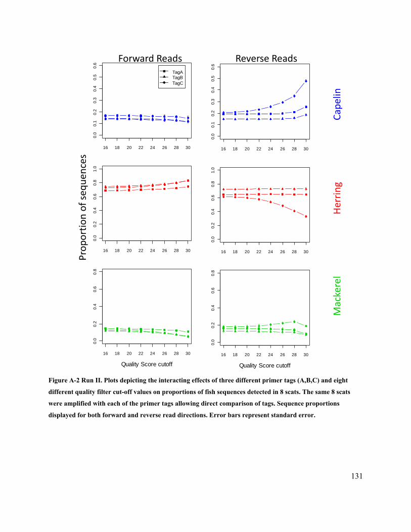
131

Figure A-2 Run II. Plots depicting the interacting effects of three different primer tags (A,B,C) and eight

different quality filter cut-off values on proportions of fish sequences detected in 8 scats. The same 8 scats

were amplified with each of the primer tags allowing direct comparison of tags. Sequence proportions

displayed for both forward and reverse read directions. Error bars represent standard error.


Capelin

Herring

Mackerel

Proportion of sequences

16 18 20 22 24 26 28 30

0.0

0.1

0.2

0.3

0.4

0.5

0.6

TagATagBTagC

16 18 20 22 24 26 28 30

0.0

0.2

0.4

0.6

0.8

1.0

16 18 20 22 24 26 28 30

0.0

0.2

0.4

0.6

0.8


16 18 20 22 24 26 28 30

0.0

0.1

0.2

0.3

0.4

0.5

0.6

16 18 20 22 24 26 28 30

0.0

0.2

0.4

0.6

0.8

1.0

16 18 20 22 24 26 28 30

0.0

0.2

0.4

0.6

0.8


132

Figure A-3 Sequence quality scores vary between species and between forward and reverse reads. Box plots

show summary of mean quality scores (median, range and upper/lower quartiles). Line plots show variation

in mean quality at specific positions along the sequence for each of target species. In (a) and (b) data are from

Run I – 90 bp; in (c) and (d) show data from Run II (note species-specific quality scores differ between runs,

possibly due to differences in sequence chemistry).

Run I - 90 bp

Run II

133

Figure A-4 Mean sequence count for each fish species for various levels of quality filtering and various

datasets (Run I – 100 bp; Run I – 90 bp; Run II). Means sequence counts calculated for forward reads and

reverse reads are shown separately.

10 15 20 25 30

050

010

0015

00

Quality score

Mea

n se

quen

ce c

ount

10 15 20 25 30

050

010

0015

00

Quality score

CapelinHerringMackerel

10 15 20 25 30

050

010

0015

00

Quality score

Mea

n se

quen

ce c

ount

10 15 20 25 30

050

010

0015

00

Quality score


10 15 20 25 30

050

010

0015

0020

00

Quality score

Mea

n se

quen

ce c

ount

10 15 20 25 30

050

010

0015

0020

00

Quality score


Run I(100 bp)

Run I(90 bp)

Run II(100 bp)


134

Appendix B Supplementary tables and figures for Chapter 5

Table B-1 Alignment of 16S fragment for salmonids in the custom reference database, showing only the polymorphic sites at their relative sequence positions.

# Species Accession number 30 43 46 47 50 54 55 57 123 124 143 153 154 155 160 163 168 169 173 181 190 201 212 213 214

1. pink salmon NC_010959.1 C − A T C G A T T A A T C C G G C T G C A A A − G

2. pink salmon AB898738.1 ∙ ∙ ∙ ∙ ∙ ∙ ∙ ∙ ∙ ∙ G ∙ ∙ ∙ ∙ ∙ ∙ ∙ ∙ ∙ ∙ ∙ ∙ ∙ ∙

3. chum salmon AP010773.1 ∙ C ∙ − ∙ ∙ ∙ C ∙ ∙ G C ∙ ∙ ∙ ∙ ∙ ∙ ∙ ∙ T ∙ ∙ ∙ A

4. chum salmon HQ592245.1 ∙ C ∙ A ∙ ∙ ∙ C ∙ ∙ G C ∙ ∙ ∙ A ∙ C ∙ ∙ ∙ ∙ ∙ ∙ A

5. sockeye salmon NC_008615.1 A C ∙ − ∙ ∙ ∙ ∙ ∙ T G C ∙ ∙ ∙ A ∙ C ∙ ∙ ∙ ∙ ∙ ∙ A

6. Chinook salmon HQ167671.1 A C ∙ C ∙ ∙ ∙ ∙ ∙ T G C ∙ ∙ ∙ A ∙ C ∙ ∙ ∙ ∙ ∙ ∙ A

7. coho salmon EF126369.1 A C ∙ C ∙ ∙ G ∙ ∙ T G C ∙ T ∙ A ∙ ∙ A ∙ ∙ ∙ ∙ ∙ A

8. steelhead GU018123.1 A C ∙ C ∙ ∙ G ∙ ∙ T G C ∙ T ∙ A ∙ ∙ A ∙ ∙ ∙ ∙ ∙ A

9. steelhead AB898746.1 A C G C ∙ ∙ ∙ ∙ ∙ T G C ∙ ∙ ∙ ∙ ∙ ∙ ∙ ∙ ∙ T G ∙ A

10. cutthroat trout KJ010735.1 A C G C ∙ ∙ ∙ ∙ ∙ T G C ∙ ∙ ∙ ∙ ∙ ∙ ∙ ∙ ∙ ∙ ∙ ∙ A

11. Dolly varden NC_000861.1 A C G ∙ A A ∙ ∙ ∙ ∙ G C ∙ ∙ ∙ ∙ ∙ ∙ ∙ ∙ T ∙ G ∙ A

12. Atlantic salmon NC_001960.1 A C G ∙ ∙ ∙ ∙ ∙ C ∙ G − − − A A T C A T T ∙ ∙ T C

135

Figure B-1 Frequency of salmon vertebrae between <2 mm and >7 mm demonstrating the size difference

between adult and juvenile salmon bones (see methods for vertebrae selection criteria). Adult and juvenile

salmon structures in seal scats can be visually differentiated in most cases by taxonomic experts.

136

Figure B-2 . Percentages of salmon (sockeye, pink, coho, chum and Chinook) by life stage (juvenile or adult)

in the diets of harbour seals using the Comox estuary haulout in 2012 and 2013. Diets were determined by

month, and the sample sizes indicate the numbers of scats collected each month. Juvenile salmon bones are

shown to dominate in the spring (Apr-Jul) and adult salmon bones in the fall (Aug - Nov), supporting the

fixed season ratio used in our decision tree classification of salmon life stages.

137

Figure B-3 Comox 2012 – monthly average percentages of salmon species (sockeye, pink, coho, chum and

Chinook) in harbour seal diet by life stage (Juv. or Ad.).

138

Figure B-4 Comox 2013 – monthly average percentages of salmon species (sockeye, pink, coho, chum and


139

Figure B-5 Fraser – summary figure for salmon in harbour seal diet, comparing DNA diet % to Hardparts

Split Sample Frequency of Occurrence (SSFO) %.

140

Figure B-6 Fraser 2012 – monthly average percentages of salmon species (sockeye, pink, coho, chum and


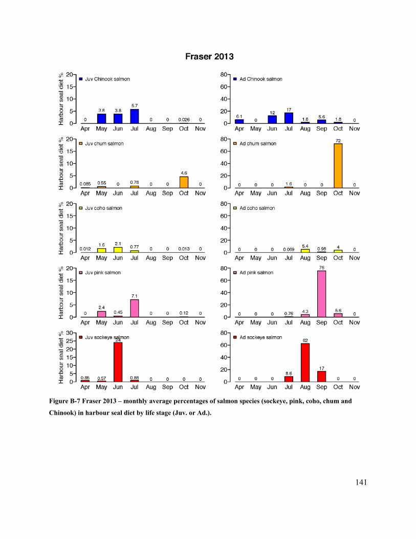
141

Figure B-7 Fraser 2013 – monthly average percentages of salmon species (sockeye, pink, coho, chum and


142

Figure B-8 Cowichan Bay– summary figure for salmon in harbour seal diet, comparing DNA diet % to

Hardparts Split Sample Frequency of Occurrence (SSFO) %.

143

Figure B-9 Cowichan Bay 2012 – monthly average percentages of salmon species (sockeye, pink, coho, chum

and Chinook) in harbour seal diet by life stage (Juv. or Ad.).

144

Figure B-10 Cowichan Bay 2013 – monthly average percentages of salmon species (sockeye, pink, coho, chum


145

Figure B-11 Belle Chain – summary figure for salmon in harbour seal diet, comparing DNA diet % to

Hardparts Split Sample Frequency of Occurrence (SSFO) %.

146

Figure B-12 Belle Chain 2012 – monthly average percentages of salmon species (sockeye, pink, coho, chum


147

Figure B-13 Belle Chain 2012 – monthly average percentages of salmon species (sockeye, pink, coho, chum


diet analysis of pacific harbour seals (phoca vitulina

Documents