developing a method for quantitative vegetable oil
TRANSCRIPT
b
DEVELOPING A METHOD FOR
QUANTITATIVE VEGETABLE OIL
ANALYSES BY MEANS OF GC-FID
Vi Bui
BACHELOR’S THESIS November 2020 Energy and Environmental Engineering Degree Programme
ABSTRACT
Tampereen ammattikorkeakoulu Tampere University of Applied Sciences Energy and Environmental Engineering Degree Programme VI BUI: Developing A Method for Quantitative Vegetable Oil Analyses by Means of GC-FID Bachelor's thesis 74 pages, appendices 14 pages December 2020
Vegetable oils in general and specialty oils in specific have an important share in human life not only because their health benefits but also because numerous industrial applications they offer. In order to explore those advantages, the need for oils quantitative analyzing is unquestionable. This paper is a part of finalizing a quantitative approach to analyze vegetable oils by GC-FID. This was done by calibrating standard solution using the already developed GC-FID method. The statistical processing of the calibration results gives parameters that will be used in future analysis of vegetable oils. There were 16 standards being calibrated in total: squalene; 4 methyl esters: me-thyl palmitate, methyl linoleate, methyl oleate and methyl stearate; 4 fatty acids: palmitic acid, linoleic acid, oleic acid, stearic acid; 𝛼-tocopherol; DL-𝛼-palmitin and a mixture of 5 triacylglycerides: tricaprylin, tricaprin, trilaurin, trimyristin, tripalmitin. By measuring the signals of one or more standard samples with known concentration of analyte, response factors (RF) were calculated. RFs of the methyl esters and squalene are slightly similar, range from 1.13 (methyl oleate) to 1.84 (methyl palmitate). A comparable fashion was found in RFs of the first three triacylglycerides: around 1.5 for tricaprylin, tricaprin and trilaurin. The RFs of other two are 2.66 for trimyristin and 3.14 for tripalmitin. Palmitic acid and DL-a-palmitin share a similar RF, approximately 3.2. A-tocopherol (vitamin E) has a small RF at 1.74. Oleic acid has a slightly bigger RF compare to others, at 3.59. The substances own the highest RFs are stearic acid (4.12) and linoleic acid (5.3). Standards retention times, their limit of detection, limit of quantification and calibration curves were also reported. The findings will provide a strong foundation for vegetable oil analysis using GC-FID. With the data collected, it is possible to indentify and quantify these chemical substances in future oils investigation.
Key words: GC-FID, quantitative analysis, specialty oils, standard calibration
3
CONTENTS
1 INTRODUCTION .................................................................................. 6
2 THEORY ............................................................................................... 9
2.1 Specialty Oils ................................................................................. 9
2.1.1 Composition ......................................................................... 9
2.1.2 Extraction ........................................................................... 19
2.1.3 Analysis .............................................................................. 21
2.2 Gas Chromatography – Flame Ionization Detector ...................... 21
2.2.1 Injector ................................................................................ 22
2.2.2 Column ............................................................................... 23
2.2.3 Detector .............................................................................. 24
2.2.4 Chromatogram.................................................................... 25
2.3 Multiple points internal standard calibration ................................. 26
2.4 LOD & LOQ .................................................................................. 27
3 MATERIAL AND METHODS .............................................................. 28
3.1 Oil extraction ................................................................................ 28
3.2 Sample preparation for GC-FID ................................................... 29
3.3 GC-FID operation ......................................................................... 30
3.4 Data processing ........................................................................... 31
3.4.1 Calibration curve ................................................................. 31
3.4.2 Response Factor ................................................................ 32
3.4.3 LOD & LOQ ........................................................................ 32
4 RESULTS ........................................................................................... 34
4.1 Squalene ...................................................................................... 34
4.2 Methyl Palmitate ........................................................................... 35
4.3 Methyl Linoleate ........................................................................... 37
4.4 Methyl Oleate ............................................................................... 39
4.5 Methyl Stearate ............................................................................ 41
4.6 Palmitic Acid................................................................................. 43
4.7 Linoleic Acid ................................................................................. 45
4.8 Oleic Acid ..................................................................................... 47
4.9 Stearic Acid .................................................................................. 48
4.10 𝛼-tocopherol .............................................................................. 50
4.11 DL-𝛼-palmitin ............................................................................. 52
4.12 TAGs mixture ............................................................................. 54
4.12.1 Tricaprylin .......................................................................... 54
4.12.2 Tricaprin ............................................................................. 56
4
4.12.3 Trilaurin .............................................................................. 57
4.12.4 Trimyristin .......................................................................... 59
4.12.5 Tripalmitin .......................................................................... 61
5 DISCUSSION ..................................................................................... 63
6 CONCLUSION .................................................................................... 66
REFERENCES ........................................................................................ 68
APPENDICES .......................................................................................... 75
Appendix 1. Squalene chromatograms signals ................................... 75
Appendix 2. Methyl Palmitate chromatograms signals........................ 76
Appendix 3. Methyl Linoleate chromatograms signals ........................ 77
Appendix 4. Methyl Oleate chromatograms signals ............................ 78
Appendix 5. Methyl Stearate chromatograms signals ......................... 79
Appendix 6. Palmitic Acid chromatograms signal ............................... 80
Appendix 7. Linoleic Acid chromatograms signals .............................. 81
Appendix 8. Oleic Acid chromatograms signals .................................. 82
Appendix 9. Stearic Acid chromatograms signals ............................... 83
Appendix 10. 𝛼-tocopherol chromatograms signals ............................ 84
Appendix 11. DL-𝛼-palmitin chromatograms signals .......................... 85
Appendix 12. Tricaprylin chromatograms signals ............................... 86
Appendix 13. Tricaprin chromatograms signals .................................. 87
Appendix 14. Trilaurin chromatograms signals ................................... 87
Appendix 15. Trimyristin chromatograms signals ............................... 88
Appendix 16. Tripalmitin chromatograms signals ............................... 88
5
ABBREVIATIONS AND TERMS
ASE Accelerated Solvent Extraction
DAG Diacylglycerol
FID Flame Ionization Detector
GC Gas Chromatography
GC-FID Gas Chromatography - Flame Ionization Detector
GC-MS Gas Chromatography - Mass Spectrometry
HPLC High Performance Liquid Chromatography
ID Inner diameter
IS Internal Standard
LOD Limit of Detection
LOQ Limit of Quantification
MAG Monoacylglycerol
MUFA Monounsaturated Fatty Acids
PUFA Polyunsaturated Fatty Acids
R2 Correlation coefficient
RF Response Factor
Rt Retention time
SFA Saturated Fatty Acids
SSL Split/Splitless
TAG Triacylglycerol
USFA Unsaturated Fatty Acids
6
1 INTRODUCTION
Vegetable fats and oils play an important role in providing essential nutrients for
living organisms in the form of food, functional foods, as raw materials for animal
feed processing and numerous other essential industries. In order to ensure the
quality of input ingredients, detecting the constituents inside the oil is not enough.
There is also a demand to understand the quantity of components. Beside con-
taminants or adulterant, which can greatly decrease oil purity, high amount of free
fatty acids in oils also indicates the oil has gone bad since free fatty acids are
precursors for peroxides and carbonyl compounds such as aldehydes and ke-
tones, which give a rancid smell to the oil (O’Brien 1998). Development of phar-
maceuticals needs quantitative analysis to measure the quality of use materials
as well as for monitoring composition of reactions over time (Rome et al. 2012).
Moreover, having an insight in the oil composition is also useful to choose proper
applications for this material. Therefore, my thesis’s objective was focused on
developing a quantitative anaylizing method for vegetable oils and fats in general.
This thesis was conducted as a part of my internship at the Centre of Expertise
on Sustainable Chemistry of Karel de Grote University of Sciences and Technol-
ogies. During my time at the Centre of Expertise, I worked on the ExtReMo project
(Specialty Oil: Extraction, Refinement and Modification). ExtReMo aim at
consulting the project’s clients with several applications for locally produced
specialty oils. In this project, a number of 'high-quality oils' will be examined. The
different crops are cultivated and processed locally by our test farms partners.
The seeds of these crops are extracted and the oils are analyzed to investigate
their usefulness in various industrial applications. In order to provide reliable
consultation to our customers, an up-to-date analyzing method to study the
quantity of oil components is required.
7
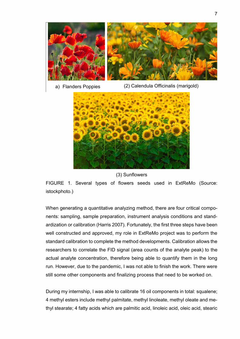
a) Flanders Poppies
(2) Calendula Officinalis (marigold)
(3) Sunflowers
FIGURE 1. Several types of flowers seeds used in ExtReMo (Source:
istockphoto.)
When generating a quantitative analyzing method, there are four critical compo-
nents: sampling, sample preparation, instrument analysis conditions and stand-
ardization or calibration (Harris 2007). Fortunately, the first three steps have been
well constructed and approved, my role in ExtReMo project was to perform the
standard calibration to complete the method developments. Calibration allows the
researchers to correlate the FID signal (area counts of the analyte peak) to the
actual analyte concentration, therefore being able to quantify them in the long
run. However, due to the pandemic, I was not able to finish the work. There were
still some other components and finalizing process that need to be worked on.
During my internship, I was able to calibrate 16 oil components in total: squalene;
4 methyl esters include methyl palmitate, methyl linoleate, methyl oleate and me-
thyl stearate; 4 fatty acids which are palmitic acid, linoleic acid, oleic acid, stearic

8
acid; 𝛼-tocopherol;DL-𝛼-palmitin and a mixture of triacylglycerides: tricaprylin, tri-
caprin, trilaurin, trimyristin, tripalmitin. Their retention times, limit of detection
(LOD), limit of quantification (LOQ), average response factors and calibration
curves were generated and presented in this report.
9
2 THEORY
2.1 Specialty Oils
Specialty Oils are vegetable oils, which contain interesting minor components
that can be used in industries. Vegetable oils are fats produced from plant-based
sources; usually from seeds, nuts, fruits and cereal grains (Hammond 2003). Our
generation witnessed a dramatic growth in vegetable oils consumptions. This is
the result of many factors including population boom, globalization, agriculture
technology, improvements of crop science, oil processing and food manufactur-
ing. Several well-known vegetable oils widely used are soybean, canola, sun-
flower and peanut. However, with an increasing demand for oils producing,
comes several concerns about complex logistic process, rigorous operations and
the stability of final products throughout the supply chain, not to mention environ-
mental impacts of oil manufacture and transportation. Moreover, the need for
specific fatty components serving different purposes has navigated current pro-
ductions trends of fats and oils. The industry is leaning towards diversify and dis-
covering new applications for vegetable oils that are locally cultivated and content
novel chemical constituents- as known as Specialty oils- by researching naturally
bred and modifying the oils to desired formula (Jung et al. 2005). This is also the
objective and orientation of ExtReMo project. In order to reach that goal, under-
standing and having an insight about oils elements is extremely crucial.
2.1.1 Composition
Vegetable oils in general and specialty oils in specific are complicated mixtures
contain mostly triacylglycerols (TAGs), which usually accounted for more than
95%. Less than 5% of the substances are diacylglycerols (DAGs) and monoacyl-
glycerols (MAGs). The other 1% are some minor components such as tocopherol,
phytosterol, etc. which give the oils their bioactive properties (Hammond 2003).
10
Glycerides
Triacylglycerols (TAGs)
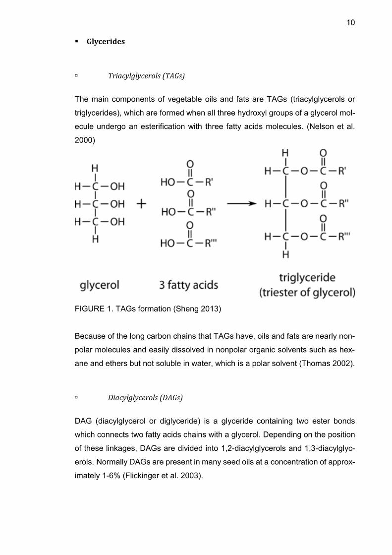
The main components of vegetable oils and fats are TAGs (triacylglycerols or
triglycerides), which are formed when all three hydroxyl groups of a glycerol mol-
ecule undergo an esterification with three fatty acids molecules. (Nelson et al.
2000)
FIGURE 1. TAGs formation (Sheng 2013)
Because of the long carbon chains that TAGs have, oils and fats are nearly non-
polar molecules and easily dissolved in nonpolar organic solvents such as hex-
ane and ethers but not soluble in water, which is a polar solvent (Thomas 2002).
Diacylglycerols (DAGs)
DAG (diacylglycerol or diglyceride) is a glyceride containing two ester bonds
which connects two fatty acids chains with a glycerol. Depending on the position
of these linkages, DAGs are divided into 1,2-diacylglycerols and 1,3-diacylglyc-
erols. Normally DAGs are present in many seed oils at a concentration of approx-
imately 1-6% (Flickinger et al. 2003).
11
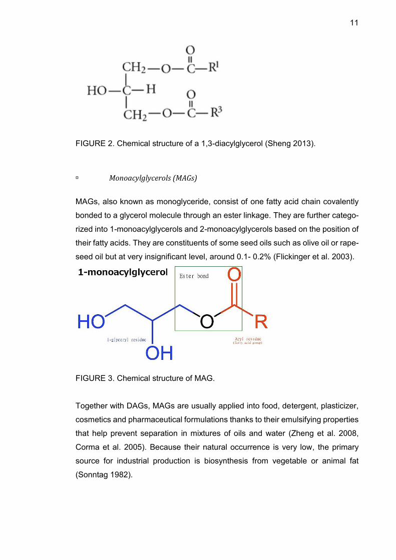
FIGURE 2. Chemical structure of a 1,3-diacylglycerol (Sheng 2013).
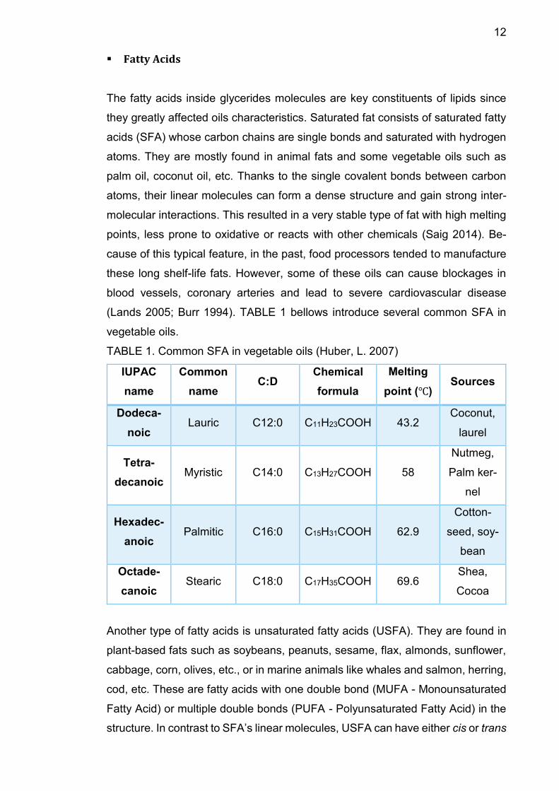
Monoacylglycerols (MAGs)
MAGs, also known as monoglyceride, consist of one fatty acid chain covalently
bonded to a glycerol molecule through an ester linkage. They are further catego-
rized into 1-monoacylglycerols and 2-monoacylglycerols based on the position of
their fatty acids. They are constituents of some seed oils such as olive oil or rape-
seed oil but at very insignificant level, around 0.1- 0.2% (Flickinger et al. 2003).
FIGURE 3. Chemical structure of MAG.
Together with DAGs, MAGs are usually applied into food, detergent, plasticizer,
cosmetics and pharmaceutical formulations thanks to their emulsifying properties
that help prevent separation in mixtures of oils and water (Zheng et al. 2008,
Corma et al. 2005). Because their natural occurrence is very low, the primary
source for industrial production is biosynthesis from vegetable or animal fat
(Sonntag 1982).
12
Fatty Acids
The fatty acids inside glycerides molecules are key constituents of lipids since
they greatly affected oils characteristics. Saturated fat consists of saturated fatty
acids (SFA) whose carbon chains are single bonds and saturated with hydrogen
atoms. They are mostly found in animal fats and some vegetable oils such as
palm oil, coconut oil, etc. Thanks to the single covalent bonds between carbon
atoms, their linear molecules can form a dense structure and gain strong inter-
molecular interactions. This resulted in a very stable type of fat with high melting
points, less prone to oxidative or reacts with other chemicals (Saig 2014). Be-
cause of this typical feature, in the past, food processors tended to manufacture
these long shelf-life fats. However, some of these oils can cause blockages in
blood vessels, coronary arteries and lead to severe cardiovascular disease
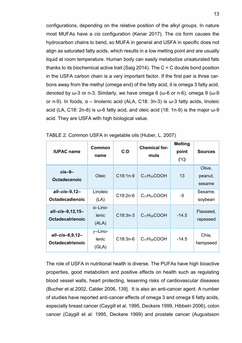
(Lands 2005; Burr 1994). TABLE 1 bellows introduce several common SFA in
vegetable oils.
TABLE 1. Common SFA in vegetable oils (Huber, L. 2007)
IUPAC
name
Common
name C:D
Chemical
formula
Melting
point (℃) Sources
Dodeca-
noic Lauric C12:0 C11H23COOH 43.2
Coconut,
laurel
Tetra-
decanoic Myristic C14:0 C13H27COOH 58
Nutmeg,
Palm ker-
nel
Hexadec-
anoic Palmitic C16:0 C15H31COOH 62.9
Cotton-
seed, soy-
bean
Octade-
canoic Stearic C18:0 C17H35COOH 69.6
Shea,
Cocoa
Another type of fatty acids is unsaturated fatty acids (USFA). They are found in
plant-based fats such as soybeans, peanuts, sesame, flax, almonds, sunflower,
cabbage, corn, olives, etc., or in marine animals like whales and salmon, herring,
cod, etc. These are fatty acids with one double bond (MUFA - Monounsaturated
Fatty Acid) or multiple double bonds (PUFA - Polyunsaturated Fatty Acid) in the
structure. In contrast to SFA’s linear molecules, USFA can have either cis or trans
13
configurations, depending on the relative position of the alkyl groups. In nature
most MUFAs have a cis configuration (Kenar 2017). The cis form causes the
hydrocarbon chains to bend, so MUFA in general and USFA in specific does not
align as saturated fatty acids, which results in a low melting point and are usually
liquid at room temperature. Human body can easily metabolize unsaturated fats
thanks to its biochemical active trait (Saig 2014). The C = C double bond position
in the USFA carbon chain is a very important factor. If the first pair is three car-
bons away from the methyl (omega end) of the fatty acid, it is omega 3 fatty acid,
denoted by ω-3 or n-3. Similarly, we have omega 6 (ω-6 or n-6), omega 9 (ω-9
or n-9). In foods, α – linolenic acid (ALA, C18: 3n-3) is ω-3 fatty acids, linoleic
acid (LA, C18: 2n-6) is ω-6 fatty acid, and oleic acid (18: 1n-9) is the major ω-9
acid. They are USFA with high biological value.
TABLE 2. Common USFA in vegetable oils (Huber, L. 2007)
IUPAC name Common
name C:D
Chemical for-
mula
Melting
point
(℃)
Sources
cis–9–
Octadecenoic Oleic C18:1n-9 C17H33COOH 13
Olive,
peanut,
sesame
all–cis–9,12–
Octadecadienoic
Linoleic
(LA) C18:2n-6 C17H31COOH -5
Sesame,
soybean
all–cis–9,12,15–
Octadecatrienoic
α–Lino-
lenic
(ALA)
C18:3n-3 C17H29COOH -14.5 Flaxseed,
rapeseed
all–cis–6,9,12–
Octadecatrienoic
𝛾–Lino-
lenic
(GLA)
C18:3n-6 C17H29COOH -14.5 Chia,
hempseed
The role of USFA in nutritional health is diverse. The PUFAs have high bioactive
properties, good metabolism and positive effects on health such as regulating
blood vessel walls, heart protecting, lessening risks of cardiovascular diseases
(Bucher et al.2002, Calder 2006, 139]. It is also an anti-cancer agent. A number
of studies have reported anti-cancer effects of omega 3 and omega 6 fatty acids,
especially breast cancer (Caygill et al. 1995, Deckere 1999, Hibbeln 2006), colon
cancer (Caygill et al. 1995, Deckere 1999) and prostate cancer (Augustsson
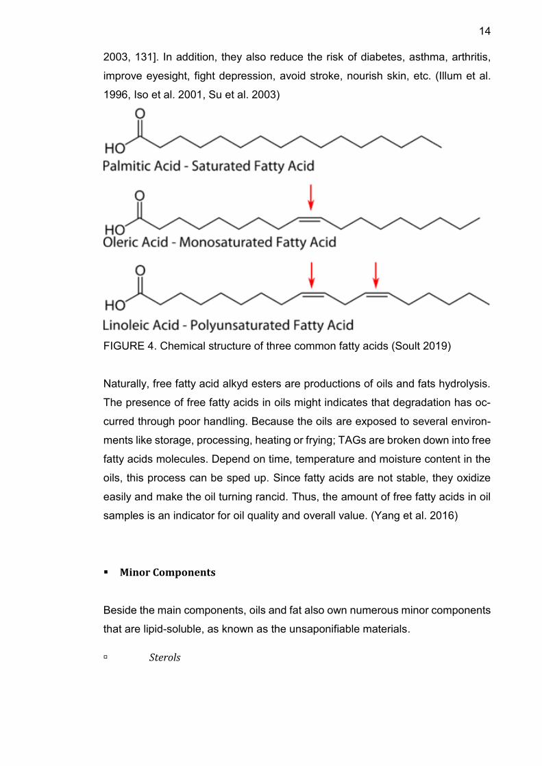
14
2003, 131]. In addition, they also reduce the risk of diabetes, asthma, arthritis,
improve eyesight, fight depression, avoid stroke, nourish skin, etc. (Illum et al.
1996, Iso et al. 2001, Su et al. 2003)
FIGURE 4. Chemical structure of three common fatty acids (Soult 2019)
Naturally, free fatty acid alkyd esters are productions of oils and fats hydrolysis.
The presence of free fatty acids in oils might indicates that degradation has oc-
curred through poor handling. Because the oils are exposed to several environ-
ments like storage, processing, heating or frying; TAGs are broken down into free
fatty acids molecules. Depend on time, temperature and moisture content in the
oils, this process can be sped up. Since fatty acids are not stable, they oxidize
easily and make the oil turning rancid. Thus, the amount of free fatty acids in oil
samples is an indicator for oil quality and overall value. (Yang et al. 2016)
Minor Components
Beside the main components, oils and fat also own numerous minor components
that are lipid-soluble, as known as the unsaponifiable materials.
Sterols
15
Sterols are the major unsaponifiable components: they are cholesterol in animal
fats and phytosterols in vegetable oils (Kamal-Eldin, A. 2013). Phytosterols with
its health benefits are recommended to increase the daily intake (Bruckert et al.
2011). The most famous and widely demonstrated is that the sterols can lower
blood levels of low-density lipoprotein, as a result, also decrease risks of heart
disease (Pollak 1953, Kritchevsky et al. 2005, Jones et al. 2009). Several studies
also claimed that these oils constituents are linked to reduced risk of cancer
(Awad et al. 2000, Woyengo et al. 2009). Phytosterols are easily found in spe-
cialty oils: rice bran oil is an outstanding example with approximately 26 mg of
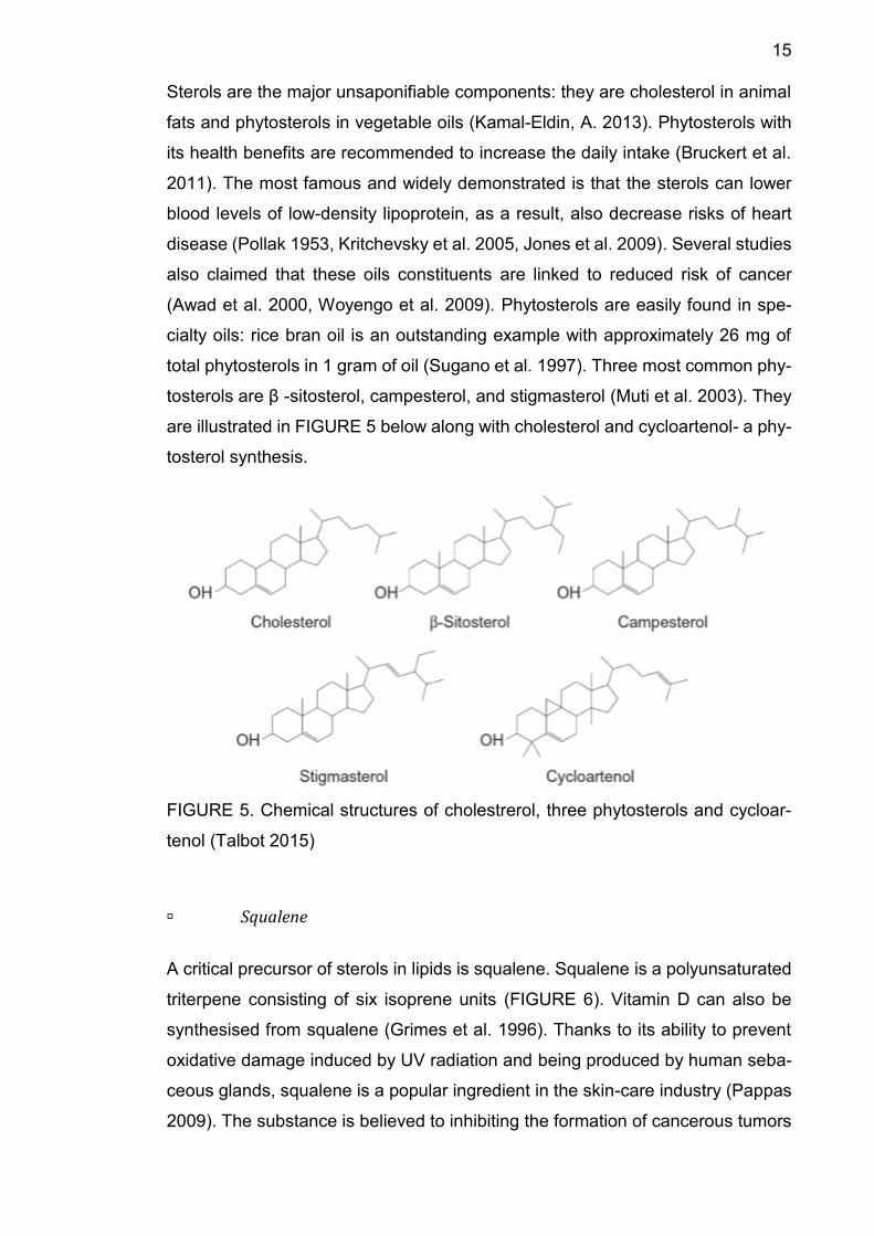
total phytosterols in 1 gram of oil (Sugano et al. 1997). Three most common phy-
tosterols are β -sitosterol, campesterol, and stigmasterol (Muti et al. 2003). They
are illustrated in FIGURE 5 below along with cholesterol and cycloartenol- a phy-
tosterol synthesis.
FIGURE 5. Chemical structures of cholestrerol, three phytosterols and cycloar-
tenol (Talbot 2015)
Squalene
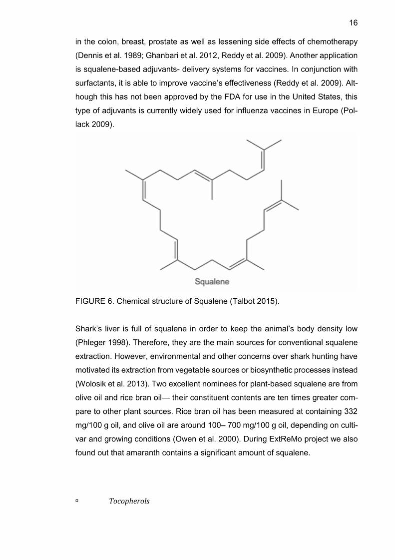
A critical precursor of sterols in lipids is squalene. Squalene is a polyunsaturated
triterpene consisting of six isoprene units (FIGURE 6). Vitamin D can also be
synthesised from squalene (Grimes et al. 1996). Thanks to its ability to prevent
oxidative damage induced by UV radiation and being produced by human seba-
ceous glands, squalene is a popular ingredient in the skin-care industry (Pappas
2009). The substance is believed to inhibiting the formation of cancerous tumors
16
in the colon, breast, prostate as well as lessening side effects of chemotherapy
(Dennis et al. 1989; Ghanbari et al. 2012, Reddy et al. 2009). Another application
is squalene-based adjuvants- delivery systems for vaccines. In conjunction with
surfactants, it is able to improve vaccine’s effectiveness (Reddy et al. 2009). Alt-
hough this has not been approved by the FDA for use in the United States, this
type of adjuvants is currently widely used for influenza vaccines in Europe (Pol-
lack 2009).
FIGURE 6. Chemical structure of Squalene (Talbot 2015).
Shark’s liver is full of squalene in order to keep the animal’s body density low
(Phleger 1998). Therefore, they are the main sources for conventional squalene
extraction. However, environmental and other concerns over shark hunting have
motivated its extraction from vegetable sources or biosynthetic processes instead
(Wolosik et al. 2013). Two excellent nominees for plant-based squalene are from
olive oil and rice bran oil— their constituent contents are ten times greater com-
pare to other plant sources. Rice bran oil has been measured at containing 332
mg/100 g oil, and olive oil are around 100– 700 mg/100 g oil, depending on culti-
var and growing conditions (Owen et al. 2000). During ExtReMo project we also
found out that amaranth contains a significant amount of squalene.
Tocopherols
17
Another ubiquitous constituent of vegetable oils that is famous for its oxidative
free radical quenching properties is tocopherol (Traber et al. 2007). Tocopherols
belong to a category of methylated phenols. They consist of four types of isomers:
the α, β, γ, and δ forms. Along with the corresponding unsaturated tocotrienol
counterparts, they are known to have Vitamin E activity (Frank 2004, Hensley et
al. 2004). Since the 1930s, it has been proved that small quantities of daily con-
sumption of vitamin E (around 15 mg) is necessary for human body function
(Fernholz 1938). Tocopherols are also associated with many health benefits, in-
cluding improvements to macular degeneration and glaucoma, reduce risk of Alz-
heimer’s and Parkinson’s disease, prevent tumor formation and limited occur-
rence of coronary heart disease (Taylor et al. 2002, Morris et al. 2005, Engin et
al. 2007, Bhupathiraju et al. 2011). Moreover, vitamin E alone or pair with vitamin
C is a famous powerful antioxidants couple that are known to minimize peroxida-
tion at the cellular level and thus help restrain premature cellular aging and tissue
degeneration (Kamal-Eldin 2013). Not only attractive to consumers, tocopherols
are also valuable for industrial use. Thanks to their capability to improve the shelf
life of oils (Choe et al. 2006, Siró et al. 2008), tocopherol can be a type of natural
preservative. In the meat industry, there are studies that show the incorporation
of tocopherols into animal feed can enhance meat quality and lifespan (Ripoll et
al. 2011, Lu et al. 2014).
18
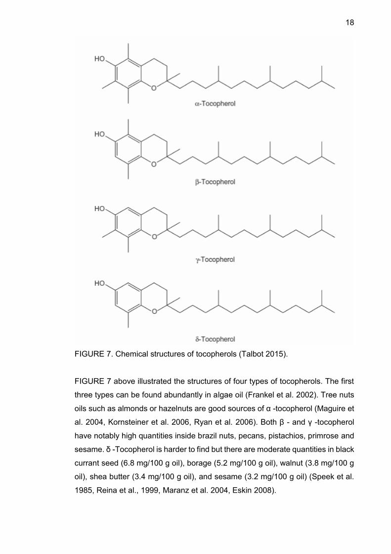
FIGURE 7. Chemical structures of tocopherols (Talbot 2015).
FIGURE 7 above illustrated the structures of four types of tocopherols. The first
three types can be found abundantly in algae oil (Frankel et al. 2002). Tree nuts
oils such as almonds or hazelnuts are good sources of α -tocopherol (Maguire et
al. 2004, Kornsteiner et al. 2006, Ryan et al. 2006). Both β - and γ -tocopherol
have notably high quantities inside brazil nuts, pecans, pistachios, primrose and
sesame. δ -Tocopherol is harder to find but there are moderate quantities in black
currant seed (6.8 mg/100 g oil), borage (5.2 mg/100 g oil), walnut (3.8 mg/100 g
oil), shea butter (3.4 mg/100 g oil), and sesame (3.2 mg/100 g oil) (Speek et al.
1985, Reina et al., 1999, Maranz et al. 2004, Eskin 2008).
19
2.1.2 Extraction
Vegetable oils are usually found in the plant seeds but also occasionally located
in other parts such as leaves or fruits. Since different fatty materials have different
oil content and properties, there are various extraction methods developed for oil
seeds in order to optimize the process by gathering maximum amount of oil from
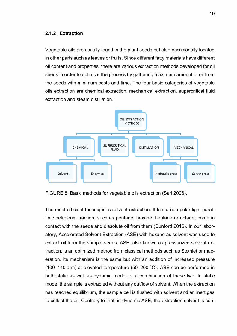
the seeds with minimum costs and time. The four basic categories of vegetable
oils extraction are chemical extraction, mechanical extraction, supercritical fluid
extraction and steam distillation.
FIGURE 8. Basic methods for vegetable oils extraction (Sari 2006).
The most efficient technique is solvent extraction. It lets a non-polar light paraf-
finic petroleum fraction, such as pentane, hexane, heptane or octane; come in
contact with the seeds and dissolute oil from them (Dunford 2016). In our labor-
atory, Accelerated Solvent Extraction (ASE) with hexane as solvent was used to
extract oil from the sample seeds. ASE, also known as pressurized solvent ex-
traction, is an optimized method from classical methods such as Soxhlet or mac-
eration. Its mechanism is the same but with an addition of increased pressure
(100–140 atm) at elevated temperature (50–200 °C). ASE can be performed in
both static as well as dynamic mode, or a combination of these two. In static
mode, the sample is extracted without any outflow of solvent. When the extraction
has reached equilibrium, the sample cell is flushed with solvent and an inert gas
to collect the oil. Contrary to that, in dynamic ASE, the extraction solvent is con-
OIL EXTRACTION METHODS
CHEMICAL
Solvent Enzymes
SUPERCRITICAL FLUID
DISTILLATION MECHANICAL
Hydraulic press Screw press
20
tinuously flowing through the extraction cell. This might resulted in higher extrac-
tion yield but also huge demand for solvent, which is not suitable for trace analysis
(Mandal et al. 2015). Therefore, static ASE was chosen for our project.
Beside extract our own oil using the ASE, ExtReMo project also received already
extracted oil by mechanical pressing from the factory. This is perhaps the oldest
and most common method of extracting oil. Through pressing, the seeds are put
under the action of compressive external forces and causing the oil to be separate
from the oleaginous material called press cake. The de-oiled cake is a high-pro-
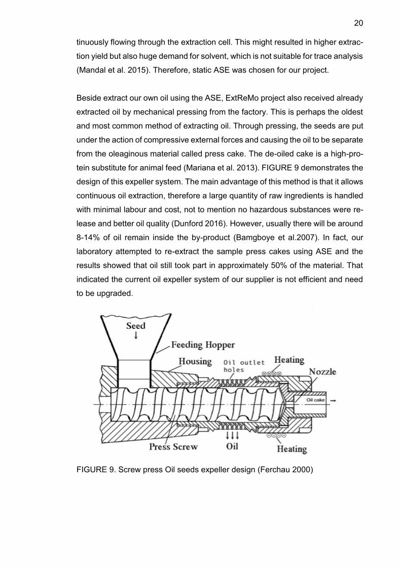
tein substitute for animal feed (Mariana et al. 2013). FIGURE 9 demonstrates the
design of this expeller system. The main advantage of this method is that it allows
continuous oil extraction, therefore a large quantity of raw ingredients is handled
with minimal labour and cost, not to mention no hazardous substances were re-
lease and better oil quality (Dunford 2016). However, usually there will be around
8-14% of oil remain inside the by-product (Bamgboye et al.2007). In fact, our
laboratory attempted to re-extract the sample press cakes using ASE and the
results showed that oil still took part in approximately 50% of the material. That
indicated the current oil expeller system of our supplier is not efficient and need
to be upgraded.
FIGURE 9. Screw press Oil seeds expeller design (Ferchau 2000)
21
2.1.3 Analysis
Currently, specialty oil analytical studies in the world mainly use chromatographic
methods. The comparison andthe selection of chromatographic method used to
suit the conditions and purposes of oil analysis is very necessary. Three most
common approaches are High Performance Liquid Chromatography (HPLC);
Gas Chromatography with Mass Spectrometry (GC-MS) and Gas Chromatog-
raphy with Flame Ionization Detector (GC-FID).
Due to the low UV absorptivity of many oil components, especially fatty acid, the
quantification range of HPLC method is limited. Creating derivatives with chro-
matophores or luminophores in order to increase detecting sensitivity can solve
this problem. Nevertheless, it can result in fronting peak or changing samples
properties because of the complicated converting process (IUPAC 1987). In con-
trast, GC-MS method provides a highly sensitive and stable qualitative analysis
based on mass spectrometry. However, the system was not used in our project.
It was due to the fact that compounds such as TAGs and DAGs are not very
volatile, thus high temperature gas chromatogramphy is needed, using special
stainless-steel columns. This cannot be combined with MS. Therefore, in the Ex-
tReMo project, GC- FID was used to analyse and quantify specialty oils.
2.2 Gas Chromatography – Flame Ionization Detector
GC is a commonly used technique in analytical chemistry for separating and ex-
amining chemical compounds that stay intact while vaporize. Its two main ele-
ments consist of an inert gaseous mobile phase and a liquid stationary phase.
Helium or other inactive gas such as nitrogen is usually use as carrier gas in
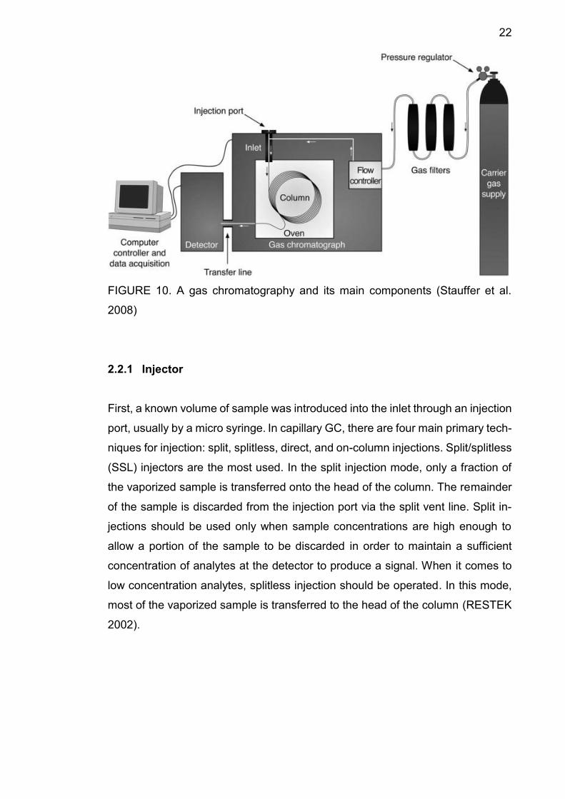
mobile phase (Pavia et al. 2006). In FIGURE 10, several basic GC units are illus-
trated.
22
FIGURE 10. A gas chromatography and its main components (Stauffer et al.
2008)
2.2.1 Injector
First, a known volume of sample was introduced into the inlet through an injection
port, usually by a micro syringe. In capillary GC, there are four main primary tech-
niques for injection: split, splitless, direct, and on-column injections. Split/splitless
(SSL) injectors are the most used. In the split injection mode, only a fraction of
the vaporized sample is transferred onto the head of the column. The remainder
of the sample is discarded from the injection port via the split vent line. Split in-
jections should be used only when sample concentrations are high enough to
allow a portion of the sample to be discarded in order to maintain a sufficient
concentration of analytes at the detector to produce a signal. When it comes to
low concentration analytes, splitless injection should be operated. In this mode,
most of the vaporized sample is transferred to the head of the column (RESTEK
2002).
23
2.2.2 Column
The mobile phase, which is carrier gas, transfers the evaporated sample from the
inlet onto the column, where the stationary phase is. The column is situated in a
temperature-controlled oven. When carrier gas with sample sweep through and
interact with column wall that is coated with stationary phase, chromatographic
separation takes place. Separated components of the sample exit the column
and immediately enter a detector in different retention time depend on its proper-
ties, which provides an electronic signal proportional to the number of eluting an-
alytes. The comparison of retention times is what gives GC its analytical useful-
ness (Stauffer et al. 2008).
Choosing the right type of column is crucial for optimizing GC separation and
analysis results. The fundamental aspects to be considered when selecting a col-
umn are its stationary phase material, inner diameter (ID), film thickness and
length. The stationary phase polarity and selectivity are concerns because they
will strongly affect the outcome. The material must share the same polarity and
selectivity with the analytes to have greater retention. Temperature limit of the
material is also crucial. Once the proper stationary phase is selected, column film
thickness and inner diameter should be optimized. The thickness (μm) of column
film directly affects both sample retention and maximum operating temperature
of the column. The thicker the film, the lower the maximum heat. Therefore, ex-
tremely volatile compounds are suitable for thick film because they will stay longer
in the column, results in more separation. In contrast, high molecular weight com-
pounds are perfect for thin film since their time in the column is shorter and pre-
vent phase bleed at higher elution temperatures. ID does not greatly impact on
retention factor like other elements, but it still plays an irreplaceable role in regu-
lating gas flow rate. Due to less mobile phase volume, small ID column (0.15 mm-
0.18 mm) generated higher retention factors in shorter analysis time, thus suita-
ble for highly complex samples. The disadvantage is that only split injections are
possilble due to the low sample loading capacity. Larger ID (0.25 mm- 0.53 mm)
can work with any kind of injection. When it comes to columns length, they are
varying from 10 to 105 meters. Longer columns provide better resolution, but they
also require more cost and analysis time. Depend on the complexity of the sam-
ple, appropriate length should be chosen (RESTEK 2013).
24
If done correctly, GC method has many advantages such as being able to analyse
all fatty acids and its methyl esters of different carbon chain length, degree of
unsaturation, position and configuration; high resolution and sensitivity, small
sample size, reliable and accurate results (Eder 1995, Shantha et al. 1992). GC
is considered to be more economical, effective and analyzing oil components in
a shorter time than HPLC method (Quiros et al. 2004).
2.2.3 Detector
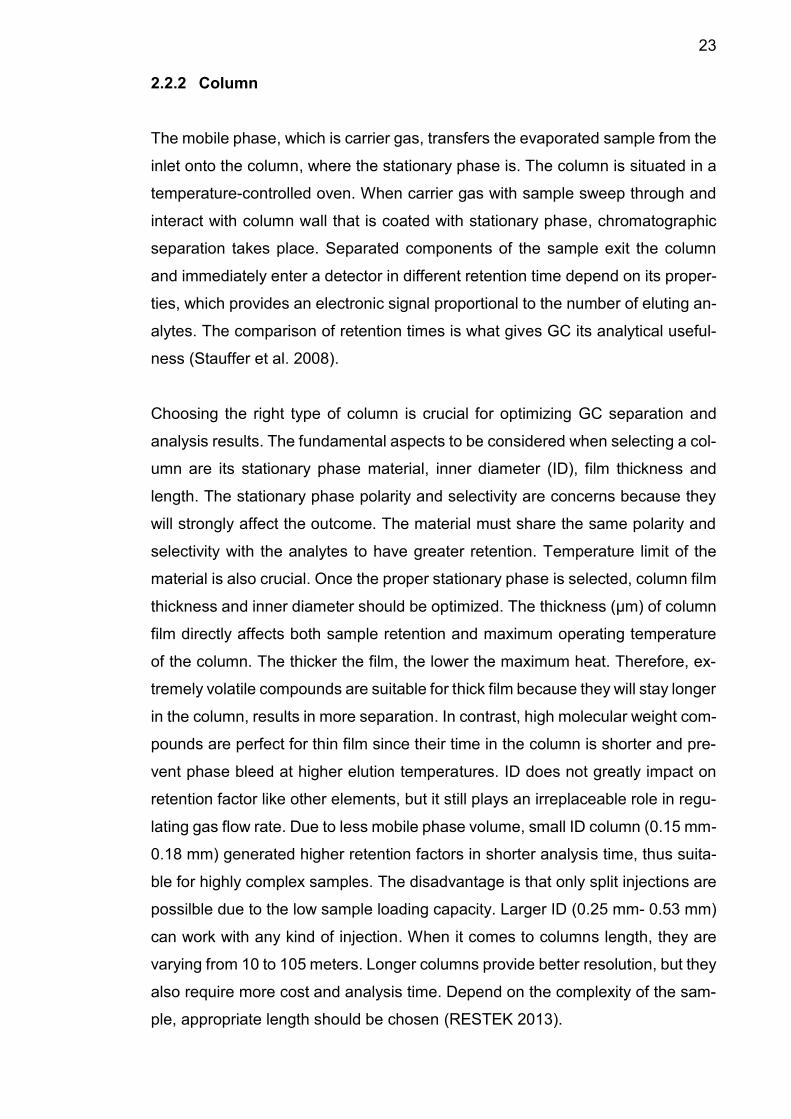
In this research, a Flame Ionization Detector (FID) was used to detect specialty
oil components. The principle of FID detector is that under the action of a flame
at high temperature (hydrogen-air flame) the ionized organic compounds, ions
and electrons move to the electrode and form electric current. The current power
is then amplified and recorded as a peak. Different components are recorded at
different time called retention time (Quiros et al. 2004, Eder 1995).
FIGURE 11. A flame ionization detector and its main components (Signal Group)
FID is one of the detectors with good sensitivity, selective with carbon-containing
organic compounds, low cost, well known with wide detectable range and high
25
stability. In fact, Capillary GC-FID is the most widely used technique for quantita-
tive oil analysis (Papazova et al. 1999). However, FID also has the disadvantages
of having to use additional gas system. Also the sample components decompose
in the flame, so sample cannot be used in the case of allowing the component to
go through another analyser (for example infrared device) and when using the
FID to analyse new substances, it is impossible to determine without standard
calibration (Eder 1995).
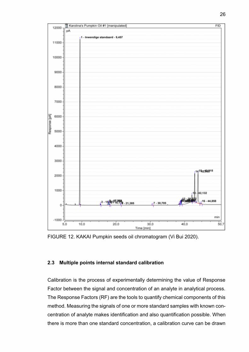
2.2.4 Chromatogram
FIGURE 12 below is an example of a type of pumpkin seeds oil’s GC-FID chro-
matogram. It illustrated the signal peaks of each components in the analyte and
their retention time. The integration results show the peaks area. From the chro-
matograms, we can visually compare the signals of different concentrations of a
component.
26
FIGURE 12. KAKAI Pumpkin seeds oil chromatogram (Vi Bui 2020).
2.3 Multiple points internal standard calibration
Calibration is the process of experimentally determining the value of Response
Factor between the signal and concentration of an analyte in analytical process.
The Response Factors (RF) are the tools to quantify chemical components of this
method. Measuring the signals of one or more standard samples with known con-
centration of analyte makes identification and also quantification possible. When
there is more than one standard concentration, a calibration curve can be drawn
27
from the results by plotting the concentration in the standard sample signal area
or height versus the signal area or height. This basic method of calibration is
called external standard calibration. However, there is noticeable amount of er-
rors so this technique is only favourable when the examining sample is simple
and small or when no instrumental variations are observed (Harvey 2016). In this
report, multiple-point internal standard calibration approach was used. It is a
more accurate calibration approach and widely used not only in chromatography
but also in quantitative HLPC-MS (Burlingame et al. 1998). An Internal Standard
(IS) is a substance, different from the analyte, added inside sample solution with
known quantity. By adding IS, the method can compensate for both instrumental
and sample preparation errors or variations because the ratios between the ana-
lytes and IS are constant (Dudley et al. 1978). Tetradecane was chosen as IS for
this project because it meets these requirements (Smith et al. 1981):
Similar in chemical structure and retention with the analyte.
Not already exist in the sample.
High purity.
Good stability.
Well resolved from the compound of interest.
2.4 LOD & LOQ
Limit of detection (LOD) and limit of quantification (LOQ) are two important per-
formance features in validating a quantitative method. They represent the small-
est concentration of an analyte that can be reliably measured by an analytical
procedure. The definitions that describe these parameters vary from different
guidelines. Likewise, there have been numerous methods for estimating it
(Shrivastava, A et al. 2011). According to European Medicines Agency, LOD is
defined as the minimum concentration that can be detected but not necessarily
quantified. Meanwhile, LOQ is the minimum analyte concentration that can be
precisely determined under the stated experimental conditions. In this paper,
LOD and LOQ were determined using visual evaluation and calibration curve
equation.
28
3 MATERIAL AND METHODS
3.1 Oil extraction
Extraction of oil from seeds consisted of 5 steps.
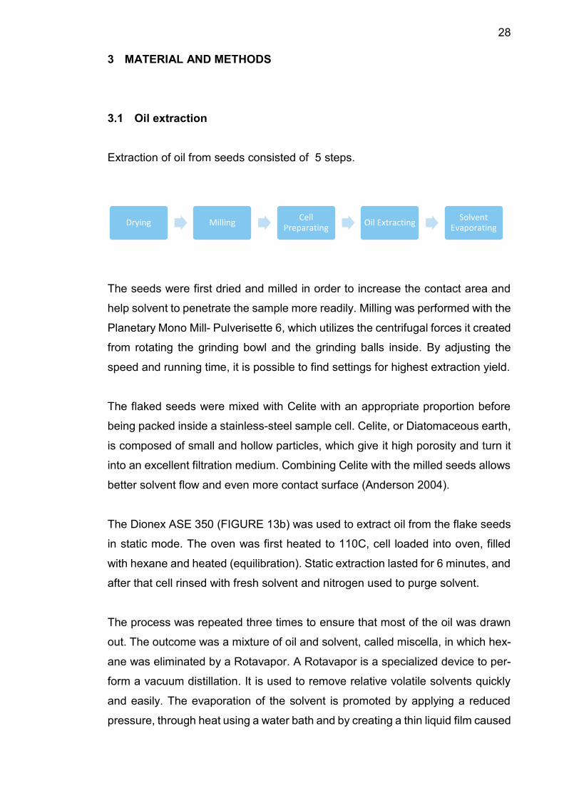
The seeds were first dried and milled in order to increase the contact area and
help solvent to penetrate the sample more readily. Milling was performed with the
Planetary Mono Mill- Pulverisette 6, which utilizes the centrifugal forces it created
from rotating the grinding bowl and the grinding balls inside. By adjusting the
speed and running time, it is possible to find settings for highest extraction yield.
The flaked seeds were mixed with Celite with an appropriate proportion before
being packed inside a stainless-steel sample cell. Celite, or Diatomaceous earth,
is composed of small and hollow particles, which give it high porosity and turn it
into an excellent filtration medium. Combining Celite with the milled seeds allows
better solvent flow and even more contact surface (Anderson 2004).
The Dionex ASE 350 (FIGURE 13b) was used to extract oil from the flake seeds
in static mode. The oven was first heated to 110C, cell loaded into oven, filled
with hexane and heated (equilibration). Static extraction lasted for 6 minutes, and
after that cell rinsed with fresh solvent and nitrogen used to purge solvent.
The process was repeated three times to ensure that most of the oil was drawn
out. The outcome was a mixture of oil and solvent, called miscella, in which hex-
ane was eliminated by a Rotavapor. A Rotavapor is a specialized device to per-
form a vacuum distillation. It is used to remove relative volatile solvents quickly
and easily. The evaporation of the solvent is promoted by applying a reduced
pressure, through heat using a water bath and by creating a thin liquid film caused
Drying MillingCell
PreparatingOil Extracting
Solvent Evaporating
29
by the spinning of the round-bottom flask. A cooler is needed for the condensation
of the evaporated gas. The final product was weighed then transferred into tightly
sealed dark glass bottle and stored in a dry cool place. Exposure to oxygen, light
or heat will subject oil to oxidation, eventually turning it rancid.
a) Pulverisette 6
b) Dionex ASE 350
c) Rotavapor
FIGURE 13. Equipment for Oil Extraction (Vi Bui 2020).
3.2 Sample preparation for GC-FID
Since GC-FID is a very accurate method with extremely sensitive detector, ana-
lytes must be diluted into a wide range of concentration, from 0.25 ppm up to
2500 ppm. In order to economically get samples with that small amount of stand-
ards, dilution procedure is divided into 2 parts: the first one in test tubes and the
second one in vials. Internal standard is diluted separately to 100 times and then
30
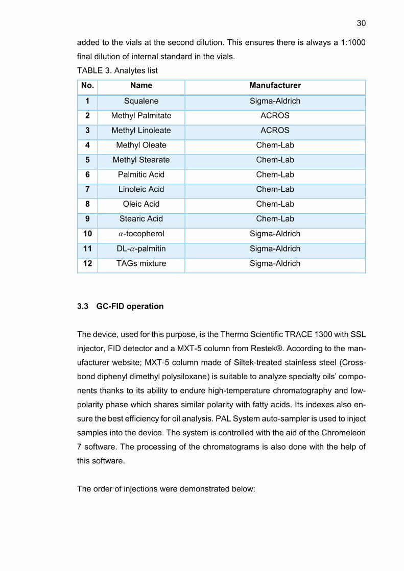
added to the vials at the second dilution. This ensures there is always a 1:1000
final dilution of internal standard in the vials.
TABLE 3. Analytes list
No. Name Manufacturer
1 Squalene Sigma-Aldrich
2 Methyl Palmitate ACROS
3 Methyl Linoleate ACROS
4 Methyl Oleate Chem-Lab
5 Methyl Stearate Chem-Lab
6 Palmitic Acid Chem-Lab
7 Linoleic Acid Chem-Lab
8 Oleic Acid Chem-Lab
9 Stearic Acid Chem-Lab
10 𝛼-tocopherol Sigma-Aldrich
11 DL-𝛼-palmitin Sigma-Aldrich
12 TAGs mixture Sigma-Aldrich
3.3 GC-FID operation
The device, used for this purpose, is the Thermo Scientific TRACE 1300 with SSL
injector, FID detector and a MXT-5 column from Restek®. According to the man-
ufacturer website; MXT-5 column made of Siltek-treated stainless steel (Cross-
bond diphenyl dimethyl polysiloxane) is suitable to analyze specialty oils’ compo-
nents thanks to its ability to endure high-temperature chromatography and low-
polarity phase which shares similar polarity with fatty acids. Its indexes also en-
sure the best efficiency for oil analysis. PAL System auto-sampler is used to inject
samples into the device. The system is controlled with the aid of the Chromeleon
7 software. The processing of the chromatograms is also done with the help of
this software.
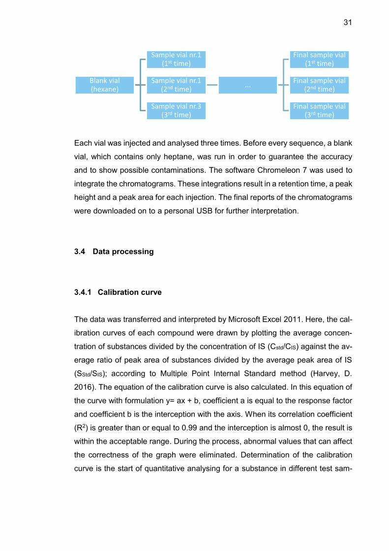
The order of injections were demonstrated below:
31
Each vial was injected and analysed three times. Before every sequence, a blank
vial, which contains only heptane, was run in order to guarantee the accuracy
and to show possible contaminations. The software Chromeleon 7 was used to
integrate the chromatograms. These integrations result in a retention time, a peak
height and a peak area for each injection. The final reports of the chromatograms
were downloaded on to a personal USB for further interpretation.
3.4 Data processing
3.4.1 Calibration curve
The data was transferred and interpreted by Microsoft Excel 2011. Here, the cal-
ibration curves of each compound were drawn by plotting the average concen-
tration of substances divided by the concentration of IS (Cstd/CIS) against the av-
erage ratio of peak area of substances divided by the average peak area of IS
(SStd/SIS); according to Multiple Point Internal Standard method (Harvey, D.
2016). The equation of the calibration curve is also calculated. In this equation of
the curve with formulation y= ax + b, coefficient a is equal to the response factor
and coefficient b is the interception with the axis. When its correlation coefficient
(R2) is greater than or equal to 0.99 and the interception is almost 0, the result is
within the acceptable range. During the process, abnormal values that can affect
the correctness of the graph were eliminated. Determination of the calibration
curve is the start of quantitative analysing for a substance in different test sam-
Blank vial (hexane)
Sample vial nr.1 (1st time)
Sample vial nr.1 (2nd time)
...
Final sample vial (1st time)
Final sample vial (2nd time)
Final sample vial (3rd time)
Sample vial nr.3 (3rd time)
32
ples. When replacing analyte’s area in calibration curve, the corresponding con-
centration can be calculated. The curve equations are also used in figuring out
Limit of Quantification.
3.4.2 Response Factor
Response Factors (RF) of each concentration were calculated using the formula
below (Harris, D.2007):
𝑅𝐹 =𝐶𝑆𝑡𝑑
𝑆𝑆𝑡𝑑×
𝑆𝐼𝑆
𝐶𝐼𝑆 (1)
Where:
RF: Response Factor
SStd : Area of analyte signal
CStd : Concentration of analyte
SIS : Area of internal standard signal
CIS : Concentration of internal standard
The average Response Factor of every concentration will be the Response Fac-
tor of the Standard.
3.4.3 LOD & LOQ
In general, the LOD of an analytical procedure is the lowest amount of analyte
present in the test sample that is detectable and does not need to be accurately
determined (European Medicines Agency, 2011). Direct technique was used to
detect the value: successively decreased the concentrations of prepared stand-
ards until the smallest visible peak. If there is a clear peak of the component in
chromatogram, that concentration is still in detection limit.
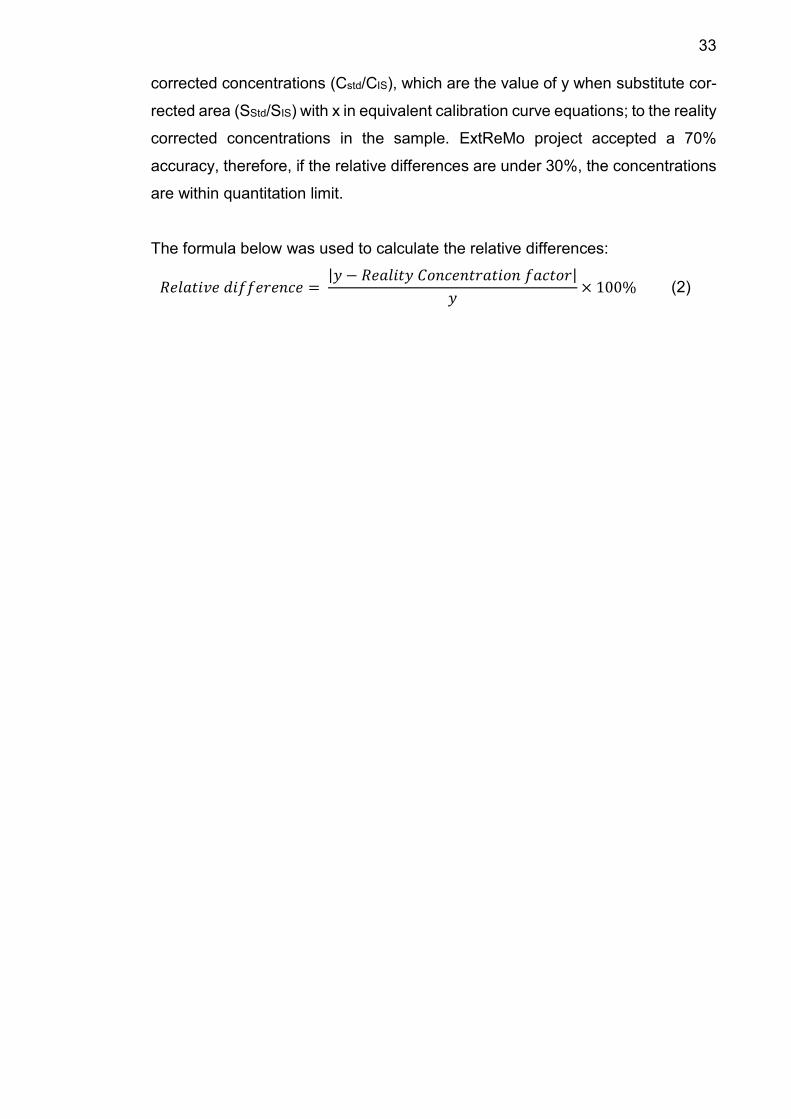
Meanwhile, LOQ is the lowest amount of analyte in the sample that can be quan-
titatively calculated with suitable precision under the stated conditions of test (Eu-
ropean Medicines Agency, 2011). It was estimated by comparing the theoretical
33
corrected concentrations (Cstd/CIS), which are the value of y when substitute cor-
rected area (SStd/SIS) with x in equivalent calibration curve equations; to the reality
corrected concentrations in the sample. ExtReMo project accepted a 70%
accuracy, therefore, if the relative differences are under 30%, the concentrations
are within quantitation limit.
The formula below was used to calculate the relative differences:
𝑅𝑒𝑙𝑎𝑡𝑖𝑣𝑒 𝑑𝑖𝑓𝑓𝑒𝑟𝑒𝑛𝑐𝑒 = |𝑦 − 𝑅𝑒𝑎𝑙𝑖𝑡𝑦 𝐶𝑜𝑛𝑐𝑒𝑛𝑡𝑟𝑎𝑡𝑖𝑜𝑛 𝑓𝑎𝑐𝑡𝑜𝑟|
𝑦× 100% (2)
34
4 RESULTS
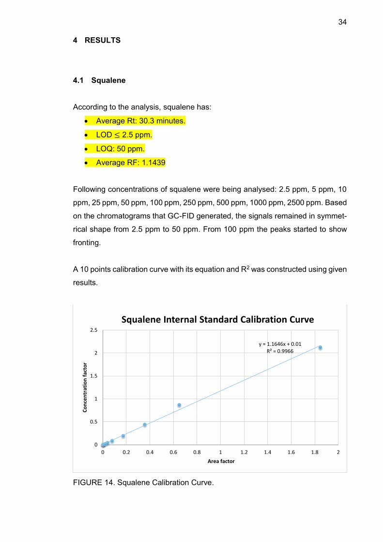
4.1 Squalene
According to the analysis, squalene has:
Average Rt: 30.3 minutes.
LOD ≤ 2.5 ppm.
LOQ: 50 ppm.
Average RF: 1.1439
Following concentrations of squalene were being analysed: 2.5 ppm, 5 ppm, 10
ppm, 25 ppm, 50 ppm, 100 ppm, 250 ppm, 500 ppm, 1000 ppm, 2500 ppm. Based
on the chromatograms that GC-FID generated, the signals remained in symmet-
rical shape from 2.5 ppm to 50 ppm. From 100 ppm the peaks started to show
fronting.
A 10 points calibration curve with its equation and R2 was constructed using given
results.
FIGURE 14. Squalene Calibration Curve.
y = 1.1646x + 0.01R² = 0.9966
0
0.5
1
1.5
2
2.5
0 0.2 0.4 0.6 0.8 1 1.2 1.4 1.6 1.8 2
Co
nce
ntr
atio
n f
acto
r
Area factor
Squalene Internal Standard Calibration Curve
35
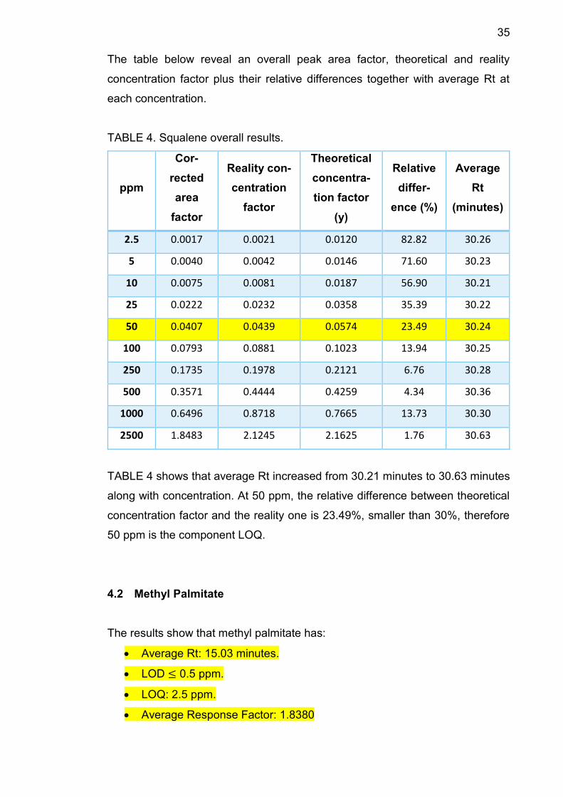
The table below reveal an overall peak area factor, theoretical and reality
concentration factor plus their relative differences together with average Rt at
each concentration.
TABLE 4. Squalene overall results.
ppm
Cor-
rected
area
factor
Reality con-
centration
factor
Theoretical
concentra-
tion factor
(y)
Relative
differ-
ence (%)
Average
Rt
(minutes)
2.5 0.0017 0.0021 0.0120 82.82 30.26
5 0.0040 0.0042 0.0146 71.60 30.23
10 0.0075 0.0081 0.0187 56.90 30.21
25 0.0222 0.0232 0.0358 35.39 30.22
50 0.0407 0.0439 0.0574 23.49 30.24
100 0.0793 0.0881 0.1023 13.94 30.25
250 0.1735 0.1978 0.2121 6.76 30.28
500 0.3571 0.4444 0.4259 4.34 30.36
1000 0.6496 0.8718 0.7665 13.73 30.30
2500 1.8483 2.1245 2.1625 1.76 30.63
TABLE 4 shows that average Rt increased from 30.21 minutes to 30.63 minutes
along with concentration. At 50 ppm, the relative difference between theoretical
concentration factor and the reality one is 23.49%, smaller than 30%, therefore
50 ppm is the component LOQ.
4.2 Methyl Palmitate
The results show that methyl palmitate has:
Average Rt: 15.03 minutes.
LOD ≤ 0.5 ppm.
LOQ: 2.5 ppm.
Average Response Factor: 1.8380
36
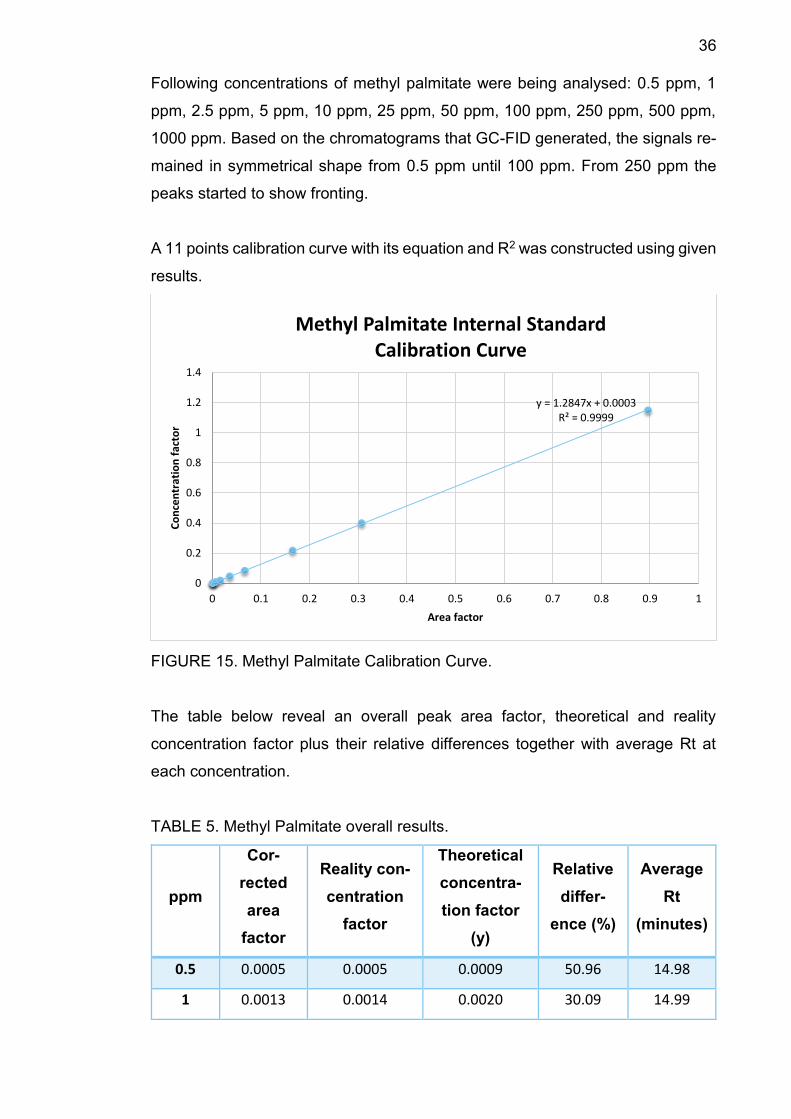
Following concentrations of methyl palmitate were being analysed: 0.5 ppm, 1
ppm, 2.5 ppm, 5 ppm, 10 ppm, 25 ppm, 50 ppm, 100 ppm, 250 ppm, 500 ppm,
1000 ppm. Based on the chromatograms that GC-FID generated, the signals re-
mained in symmetrical shape from 0.5 ppm until 100 ppm. From 250 ppm the
peaks started to show fronting.
A 11 points calibration curve with its equation and R2 was constructed using given
results.
FIGURE 15. Methyl Palmitate Calibration Curve.
The table below reveal an overall peak area factor, theoretical and reality
concentration factor plus their relative differences together with average Rt at
each concentration.
TABLE 5. Methyl Palmitate overall results.
ppm
Cor-
rected
area
factor
Reality con-
centration
factor
Theoretical
concentra-
tion factor
(y)
Relative
differ-
ence (%)
Average
Rt
(minutes)
0.5 0.0005 0.0005 0.0009 50.96 14.98
1 0.0013 0.0014 0.0020 30.09 14.99
y = 1.2847x + 0.0003R² = 0.9999
0
0.2
0.4
0.6
0.8
1
1.2
1.4
0 0.1 0.2 0.3 0.4 0.5 0.6 0.7 0.8 0.9 1
Co
nce
ntr
atio
n f
acto
r
Area factor
Methyl Palmitate Internal Standard Calibration Curve
37
2.5 0.0017 0.0021 0.0025 15.11 15.01
5 0.0041 0.0039 0.0055 28.41 15.01
10 0.0072 0.0089 0.0095 6.91 15.01
25 0.0167 0.0199 0.0218 8.57 15.01
50 0.0360 0.0466 0.0465 0.18 15.01
100 0.0669 0.0838 0.0862 2.84 15.02
250 0.1653 0.2179 0.2127 2.46 15.06
500 0.3073 0.4002 0.3950 1.32 15.08
1000 0.8962 1.1492 1.1517 0.22 15.16
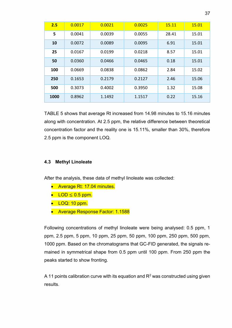
TABLE 5 shows that average Rt increased from 14.98 minutes to 15.16 minutes
along with concentration. At 2.5 ppm, the relative difference between theoretical
concentration factor and the reality one is 15.11%, smaller than 30%, therefore
2.5 ppm is the component LOQ.
4.3 Methyl Linoleate
After the analysis, these data of methyl linoleate was collected:
Average Rt: 17.04 minutes.
LOD ≤ 0.5 ppm.
LOQ: 10 ppm.
Average Response Factor: 1.1588
Following concentrations of methyl linoleate were being analysed: 0.5 ppm, 1
ppm, 2.5 ppm, 5 ppm, 10 ppm, 25 ppm, 50 ppm, 100 ppm, 250 ppm, 500 ppm,
1000 ppm. Based on the chromatograms that GC-FID generated, the signals re-
mained in symmetrical shape from 0.5 ppm until 100 ppm. From 250 ppm the
peaks started to show fronting.
A 11 points calibration curve with its equation and R2 was constructed using given
results.
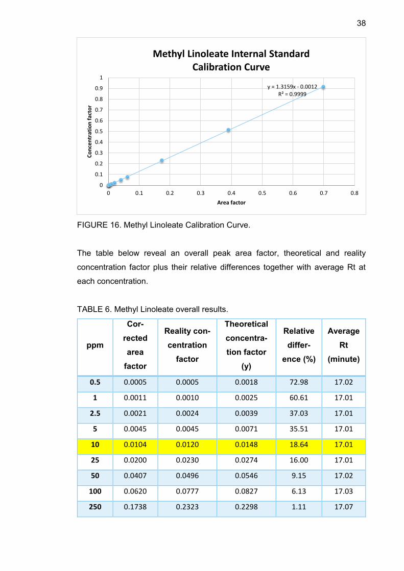
38
FIGURE 16. Methyl Linoleate Calibration Curve.
The table below reveal an overall peak area factor, theoretical and reality
concentration factor plus their relative differences together with average Rt at
each concentration.
TABLE 6. Methyl Linoleate overall results.
ppm
Cor-
rected
area
factor
Reality con-
centration
factor
Theoretical
concentra-
tion factor
(y)
Relative
differ-
ence (%)
Average
Rt
(minute)
0.5 0.0005 0.0005 0.0018 72.98 17.02
1 0.0011 0.0010 0.0025 60.61 17.01
2.5 0.0021 0.0024 0.0039 37.03 17.01
5 0.0045 0.0045 0.0071 35.51 17.01
10 0.0104 0.0120 0.0148 18.64 17.01
25 0.0200 0.0230 0.0274 16.00 17.01
50 0.0407 0.0496 0.0546 9.15 17.02
100 0.0620 0.0777 0.0827 6.13 17.03
250 0.1738 0.2323 0.2298 1.11 17.07
y = 1.3159x - 0.0012R² = 0.9999
0
0.1
0.2
0.3
0.4
0.5
0.6
0.7
0.8
0.9
1
0 0.1 0.2 0.3 0.4 0.5 0.6 0.7 0.8
Co
nce
ntr
atio
n f
acto
r
Area factor
Methyl Linoleate Internal Standard Calibration Curve
39
500 0.3904 0.5160 0.5148 0.23 17.12
1000 0.6989 0.9159 0.9208 0.54 17.18
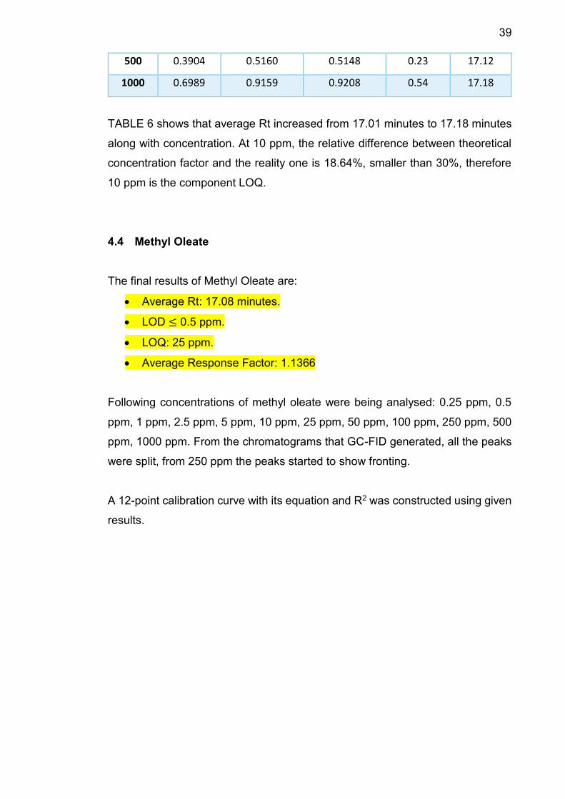
TABLE 6 shows that average Rt increased from 17.01 minutes to 17.18 minutes
along with concentration. At 10 ppm, the relative difference between theoretical
concentration factor and the reality one is 18.64%, smaller than 30%, therefore
10 ppm is the component LOQ.
4.4 Methyl Oleate
The final results of Methyl Oleate are:
Average Rt: 17.08 minutes.
LOD ≤ 0.5 ppm.
LOQ: 25 ppm.
Average Response Factor: 1.1366
Following concentrations of methyl oleate were being analysed: 0.25 ppm, 0.5
ppm, 1 ppm, 2.5 ppm, 5 ppm, 10 ppm, 25 ppm, 50 ppm, 100 ppm, 250 ppm, 500
ppm, 1000 ppm. From the chromatograms that GC-FID generated, all the peaks
were split, from 250 ppm the peaks started to show fronting.
A 12-point calibration curve with its equation and R2 was constructed using given
results.

40
FIGURE 17. Methyl Oleate Calibration Curve.
The table below reveal an overall peak area factor, theoretical and reality
concentration factor plus their relative differences together with average Rt at
each concentration.
TABLE 7. Methyl Oleate overall results.
ppm
Cor-
rected
area
factor
Reality con-
centration
factor
Theoretical
concentra-
tion factor
(y)
Relative
differ-
ence (%)
Average
Rt
(minutes)
0.5 0.0007 0.0005 0.0039 87.51 17.05
1 0.0013 0.0011 0.0048 77.92 17.04
2.5 0.0027 0.0026 0.0068 61.17 17.04
5 0.0053 0.0057 0.0108 47.20 17.04
10 0.0094 0.0112 0.0170 33.90 17.05
25 0.0224 0.0280 0.0366 23.59 17.05
50 0.0407 0.0528 0.0642 17.69 17.06
100 0.0778 0.1039 0.1200 13.44 17.08
250 0.1532 0.2470 0.2337 5.69 17.08
y = 1.5074x - 0.0028R² = 0.9994
0
0.2
0.4
0.6
0.8
1
1.2
0 0.1 0.2 0.3 0.4 0.5 0.6 0.7 0.8
Co
nce
ntr
atio
n f
acto
r
Area factor
Methyl Oleate Internal Standard Calibration Curve
41
500 0.3423 0.5021 0.5189 3.23 17.15
1000 0.6914 1.0423 1.0450 0.26 17.19
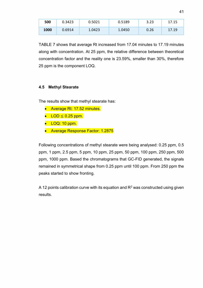
TABLE 7 shows that average Rt increased from 17.04 minutes to 17.19 minutes
along with concentration. At 25 ppm, the relative difference between theoretical
concentration factor and the reality one is 23.59%, smaller than 30%, therefore
25 ppm is the component LOQ.
4.5 Methyl Stearate
The results show that methyl stearate has:
Average Rt: 17.52 minutes.
LOD ≤ 0.25 ppm.
LOQ: 10 ppm.
Average Response Factor: 1.2875
Following concentrations of methyl stearate were being analysed: 0.25 ppm, 0.5
ppm, 1 ppm, 2.5 ppm, 5 ppm, 10 ppm, 25 ppm, 50 ppm, 100 ppm, 250 ppm, 500
ppm, 1000 ppm. Based the chromatograms that GC-FID generated, the signals
remained in symmetrical shape from 0.25 ppm until 100 ppm. From 250 ppm the
peaks started to show fronting.
A 12 points calibration curve with its equation and R2 was constructed using given
results.
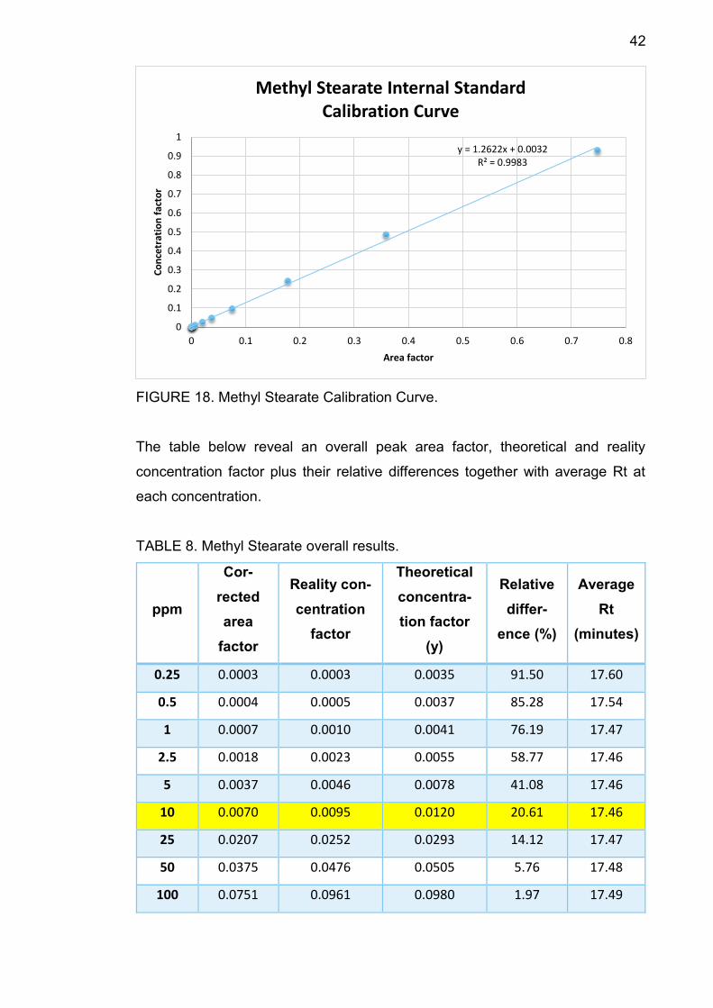
42
FIGURE 18. Methyl Stearate Calibration Curve.
The table below reveal an overall peak area factor, theoretical and reality
concentration factor plus their relative differences together with average Rt at
each concentration.
TABLE 8. Methyl Stearate overall results.
ppm
Cor-
rected
area
factor
Reality con-
centration
factor
Theoretical
concentra-
tion factor
(y)
Relative
differ-
ence (%)
Average
Rt
(minutes)
0.25 0.0003 0.0003 0.0035 91.50 17.60
0.5 0.0004 0.0005 0.0037 85.28 17.54
1 0.0007 0.0010 0.0041 76.19 17.47
2.5 0.0018 0.0023 0.0055 58.77 17.46
5 0.0037 0.0046 0.0078 41.08 17.46
10 0.0070 0.0095 0.0120 20.61 17.46
25 0.0207 0.0252 0.0293 14.12 17.47
50 0.0375 0.0476 0.0505 5.76 17.48
100 0.0751 0.0961 0.0980 1.97 17.49
y = 1.2622x + 0.0032R² = 0.9983
0
0.1
0.2
0.3
0.4
0.5
0.6
0.7
0.8
0.9
1
0 0.1 0.2 0.3 0.4 0.5 0.6 0.7 0.8
Co
nce
trat
ion
fac
tor
Area factor
Methyl Stearate Internal Standard Calibration Curve
43
250 0.1777 0.2422 0.2275 6.43 17.54
500 0.3587 0.4865 0.4560 6.71 17.59
1000 0.7483 0.9301 0.9477 1.85 17.68
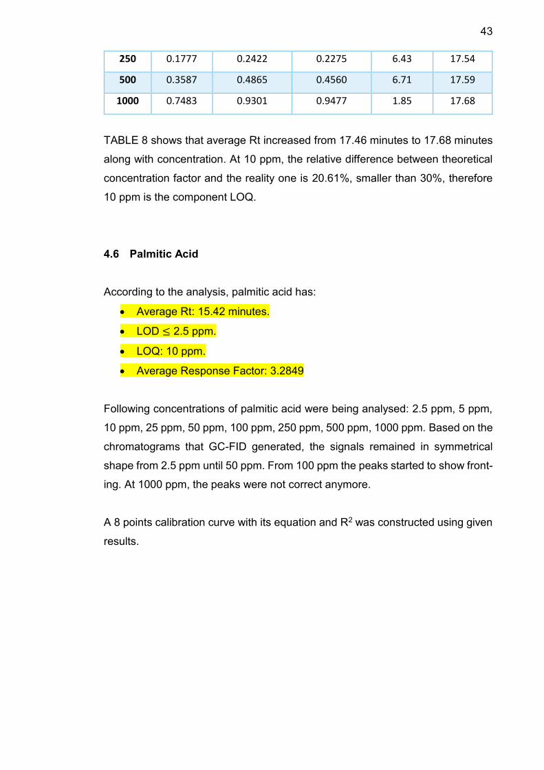
TABLE 8 shows that average Rt increased from 17.46 minutes to 17.68 minutes
along with concentration. At 10 ppm, the relative difference between theoretical
concentration factor and the reality one is 20.61%, smaller than 30%, therefore
10 ppm is the component LOQ.
4.6 Palmitic Acid
According to the analysis, palmitic acid has:
Average Rt: 15.42 minutes.
LOD ≤ 2.5 ppm.
LOQ: 10 ppm.
Average Response Factor: 3.2849
Following concentrations of palmitic acid were being analysed: 2.5 ppm, 5 ppm,
10 ppm, 25 ppm, 50 ppm, 100 ppm, 250 ppm, 500 ppm, 1000 ppm. Based on the
chromatograms that GC-FID generated, the signals remained in symmetrical
shape from 2.5 ppm until 50 ppm. From 100 ppm the peaks started to show front-
ing. At 1000 ppm, the peaks were not correct anymore.
A 8 points calibration curve with its equation and R2 was constructed using given
results.
44
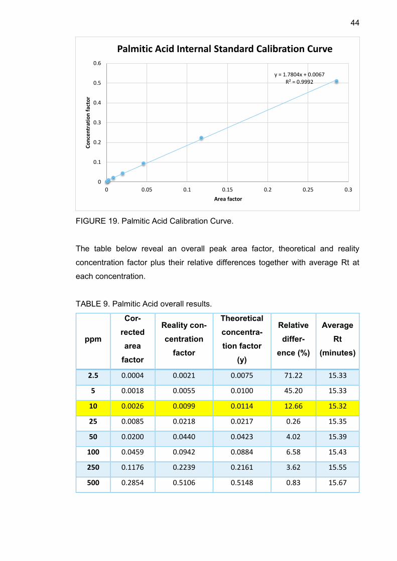
FIGURE 19. Palmitic Acid Calibration Curve.
The table below reveal an overall peak area factor, theoretical and reality
concentration factor plus their relative differences together with average Rt at
each concentration.
TABLE 9. Palmitic Acid overall results.
ppm
Cor-
rected
area
factor
Reality con-
centration
factor
Theoretical
concentra-
tion factor
(y)
Relative
differ-
ence (%)
Average
Rt
(minutes)
2.5 0.0004 0.0021 0.0075 71.22 15.33
5 0.0018 0.0055 0.0100 45.20 15.33
10 0.0026 0.0099 0.0114 12.66 15.32
25 0.0085 0.0218 0.0217 0.26 15.35
50 0.0200 0.0440 0.0423 4.02 15.39
100 0.0459 0.0942 0.0884 6.58 15.43
250 0.1176 0.2239 0.2161 3.62 15.55
500 0.2854 0.5106 0.5148 0.83 15.67
y = 1.7804x + 0.0067R² = 0.9992
0
0.1
0.2
0.3
0.4
0.5
0.6
0 0.05 0.1 0.15 0.2 0.25 0.3
Co
nce
ntr
atio
n f
acto
r
Area factor
Palmitic Acid Internal Standard Calibration Curve
45
TABLE 9 shows that average Rt increased from 15.32 minutes to 15.67 minutes
along with concentration. At 10 ppm, the relative difference between theoretical
concentration factor and the reality one is 12.66%, smaller than 30%, therefore
10 ppm is the component LOQ.
4.7 Linoleic Acid
The results show that linoleic acid has:
Average Rt: 17.62 minutes.
LOD: 2.5 ppm.
LOQ: 10 ppm.
Average Response Factor: 5.2979
Following concentrations of linoleic acid were being analysed: 1 ppm, 2.5 ppm, 5
ppm, 10 ppm, 25 ppm, 50 ppm, 100 ppm, 250 ppm, 500 ppm, 1000 ppm. There
was no peak detected at 1 ppm. Based on the chromatograms that GC-FID gen-
erated, first three concentration resulted in tailing peaks, the signals remained in
symmetrical shape from 25 ppm until 100 ppm, the peaks became fronting start-
ing at 250 ppm. At 1000 ppm, the peaks were not correct anymore.
A 8 points calibration curve with its equation and R2 was constructed using given
results.
46
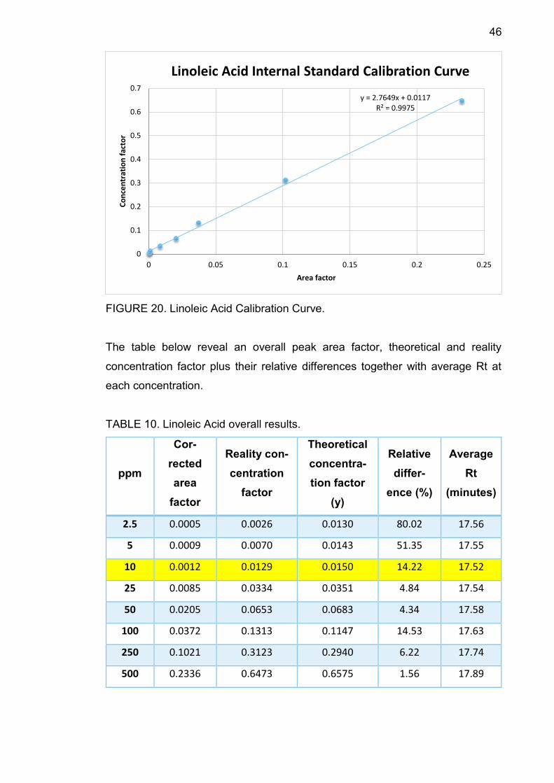
FIGURE 20. Linoleic Acid Calibration Curve.
The table below reveal an overall peak area factor, theoretical and reality
concentration factor plus their relative differences together with average Rt at
each concentration.
TABLE 10. Linoleic Acid overall results.
ppm
Cor-
rected
area
factor
Reality con-
centration
factor
Theoretical
concentra-
tion factor
(y)
Relative
differ-
ence (%)
Average
Rt
(minutes)
2.5 0.0005 0.0026 0.0130 80.02 17.56
5 0.0009 0.0070 0.0143 51.35 17.55
10 0.0012 0.0129 0.0150 14.22 17.52
25 0.0085 0.0334 0.0351 4.84 17.54
50 0.0205 0.0653 0.0683 4.34 17.58
100 0.0372 0.1313 0.1147 14.53 17.63
250 0.1021 0.3123 0.2940 6.22 17.74
500 0.2336 0.6473 0.6575 1.56 17.89
y = 2.7649x + 0.0117R² = 0.9975
0
0.1
0.2
0.3
0.4
0.5
0.6
0.7
0 0.05 0.1 0.15 0.2 0.25
Co
nce
ntr
atio
n f
acto
r
Area factor
Linoleic Acid Internal Standard Calibration Curve
47
TABLE 10 shows that average Rt increased from 17.52 minutes to 17.89 minutes
along with concentration. At 10 ppm, the relative difference between theoretical
concentration factor and the reality one is 14.22%, smaller than 30%, therefore
10 ppm is the component LOQ.
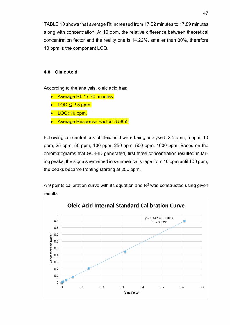
4.8 Oleic Acid
According to the analysis, oleic acid has:
Average Rt: 17.70 minutes.
LOD ≤ 2.5 ppm.
LOQ: 10 ppm.
Average Response Factor: 3.5855
Following concentrations of oleic acid were being analysed: 2.5 ppm, 5 ppm, 10
ppm, 25 ppm, 50 ppm, 100 ppm, 250 ppm, 500 ppm, 1000 ppm. Based on the
chromatograms that GC-FID generated, first three concentration resulted in tail-
ing peaks, the signals remained in symmetrical shape from 10 ppm until 100 ppm,
the peaks became fronting starting at 250 ppm.
A 9 points calibration curve with its equation and R2 was constructed using given
results.
y = 1.4478x + 0.0068R² = 0.9995
0
0.1
0.2
0.3
0.4
0.5
0.6
0.7
0.8
0.9
1
0 0.1 0.2 0.3 0.4 0.5 0.6 0.7
Co
nce
ntr
atio
n f
acto
r
Area factor
Oleic Acid Internal Standard Calibration Curve
48
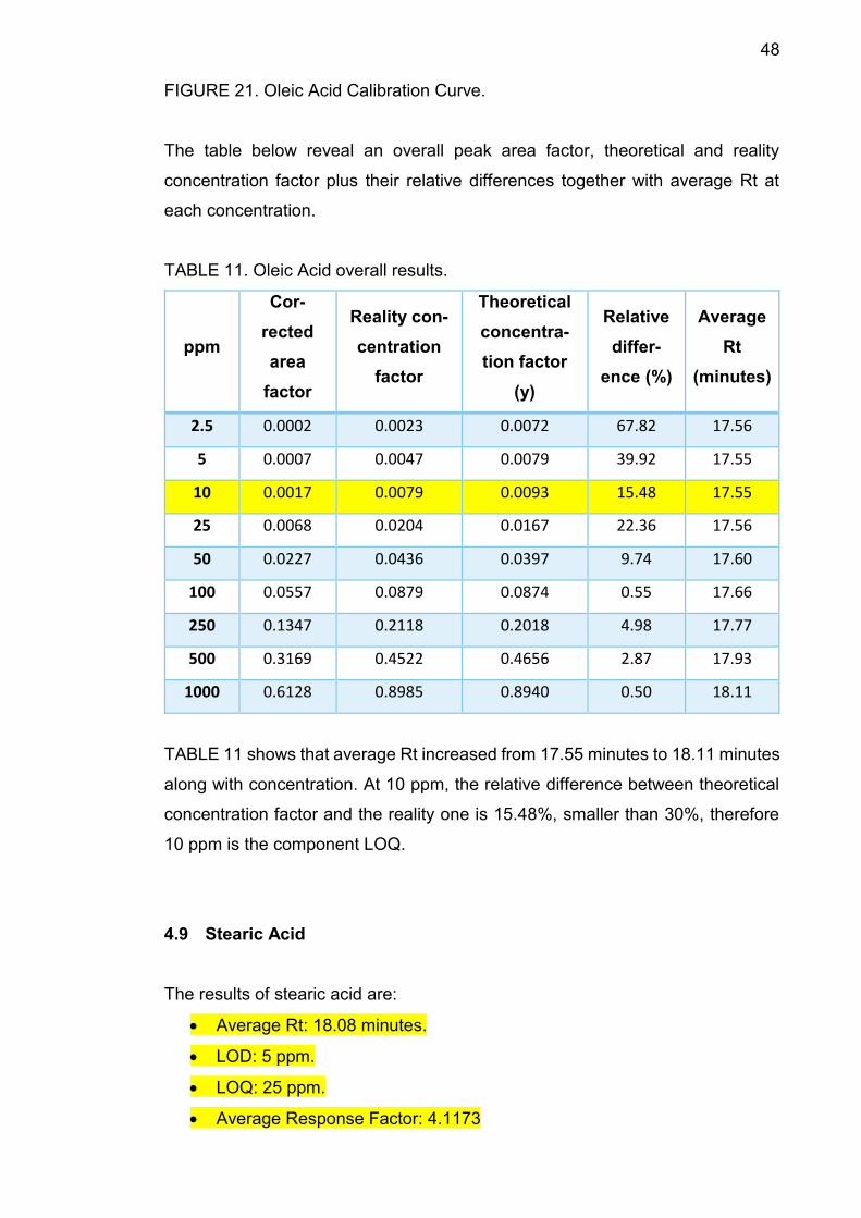
FIGURE 21. Oleic Acid Calibration Curve.
The table below reveal an overall peak area factor, theoretical and reality
concentration factor plus their relative differences together with average Rt at
each concentration.
TABLE 11. Oleic Acid overall results.
ppm
Cor-
rected
area
factor
Reality con-
centration
factor
Theoretical
concentra-
tion factor
(y)
Relative
differ-
ence (%)
Average
Rt
(minutes)
2.5 0.0002 0.0023 0.0072 67.82 17.56
5 0.0007 0.0047 0.0079 39.92 17.55
10 0.0017 0.0079 0.0093 15.48 17.55
25 0.0068 0.0204 0.0167 22.36 17.56
50 0.0227 0.0436 0.0397 9.74 17.60
100 0.0557 0.0879 0.0874 0.55 17.66
250 0.1347 0.2118 0.2018 4.98 17.77
500 0.3169 0.4522 0.4656 2.87 17.93
1000 0.6128 0.8985 0.8940 0.50 18.11
TABLE 11 shows that average Rt increased from 17.55 minutes to 18.11 minutes
along with concentration. At 10 ppm, the relative difference between theoretical
concentration factor and the reality one is 15.48%, smaller than 30%, therefore
10 ppm is the component LOQ.
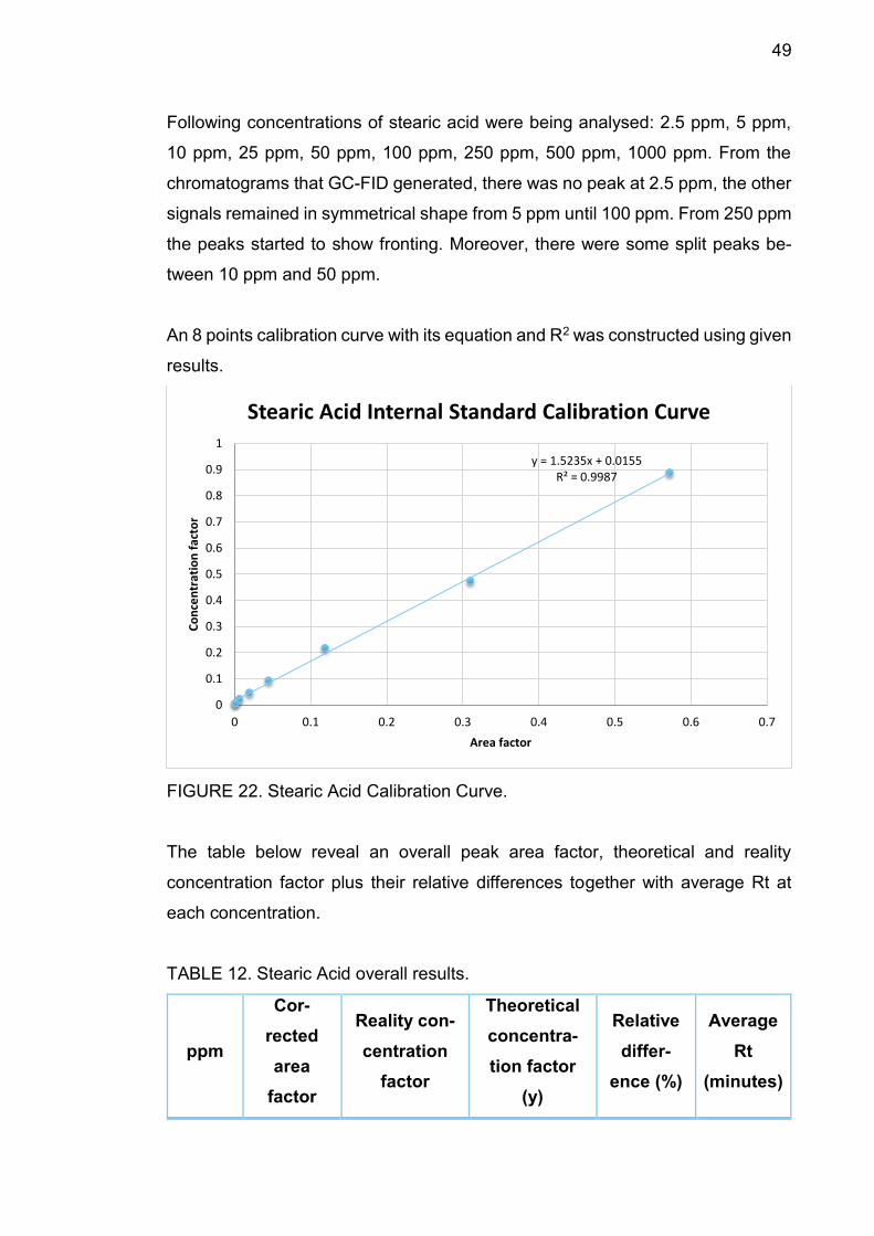
4.9 Stearic Acid
The results of stearic acid are:
Average Rt: 18.08 minutes.
LOD: 5 ppm.
LOQ: 25 ppm.
Average Response Factor: 4.1173
49
Following concentrations of stearic acid were being analysed: 2.5 ppm, 5 ppm,
10 ppm, 25 ppm, 50 ppm, 100 ppm, 250 ppm, 500 ppm, 1000 ppm. From the
chromatograms that GC-FID generated, there was no peak at 2.5 ppm, the other
signals remained in symmetrical shape from 5 ppm until 100 ppm. From 250 ppm
the peaks started to show fronting. Moreover, there were some split peaks be-
tween 10 ppm and 50 ppm.
An 8 points calibration curve with its equation and R2 was constructed using given
results.
FIGURE 22. Stearic Acid Calibration Curve.
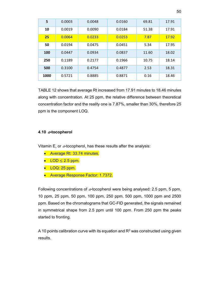
The table below reveal an overall peak area factor, theoretical and reality
concentration factor plus their relative differences together with average Rt at
each concentration.
TABLE 12. Stearic Acid overall results.
ppm
Cor-
rected
area
factor
Reality con-
centration
factor
Theoretical
concentra-
tion factor
(y)
Relative
differ-
ence (%)
Average
Rt
(minutes)
y = 1.5235x + 0.0155R² = 0.9987
0
0.1
0.2
0.3
0.4
0.5
0.6
0.7
0.8
0.9
1
0 0.1 0.2 0.3 0.4 0.5 0.6 0.7
Co
nce
ntr
atio
n f
acto
r
Area factor
Stearic Acid Internal Standard Calibration Curve
50
5 0.0003 0.0048 0.0160 69.81 17.91
10 0.0019 0.0090 0.0184 51.38 17.91
25 0.0064 0.0233 0.0253 7.87 17.92
50 0.0194 0.0475 0.0451 5.34 17.95
100 0.0447 0.0934 0.0837 11.60 18.02
250 0.1189 0.2177 0.1966 10.75 18.14
500 0.3100 0.4754 0.4877 2.53 18.31
1000 0.5721 0.8885 0.8871 0.16 18.46
TABLE 12 shows that average Rt increased from 17.91 minutes to 18.46 minutes
along with concentration. At 25 ppm, the relative difference between theoretical
concentration factor and the reality one is 7.87%, smaller than 30%, therefore 25
ppm is the component LOQ.
4.10 𝛼-tocopherol
Vitamin E, or 𝛼-tocopherol, has these results after the analysis:
Average Rt: 33.74 minutes.
LOD ≤ 2.5 ppm.
LOQ: 25 ppm.
Average Response Factor: 1.7372.
Following concentrations of 𝛼-tocopherol were being analysed: 2.5 ppm, 5 ppm,
10 ppm, 25 ppm, 50 ppm, 100 ppm, 250 ppm, 500 ppm, 1000 ppm and 2500
ppm. Based on the chromatograms that GC-FID generated, the signals remained
in symmetrical shape from 2.5 ppm until 100 ppm. From 250 ppm the peaks
started to fronting.
A 10 points calibration curve with its equation and R2 was constructed using given
results.
51
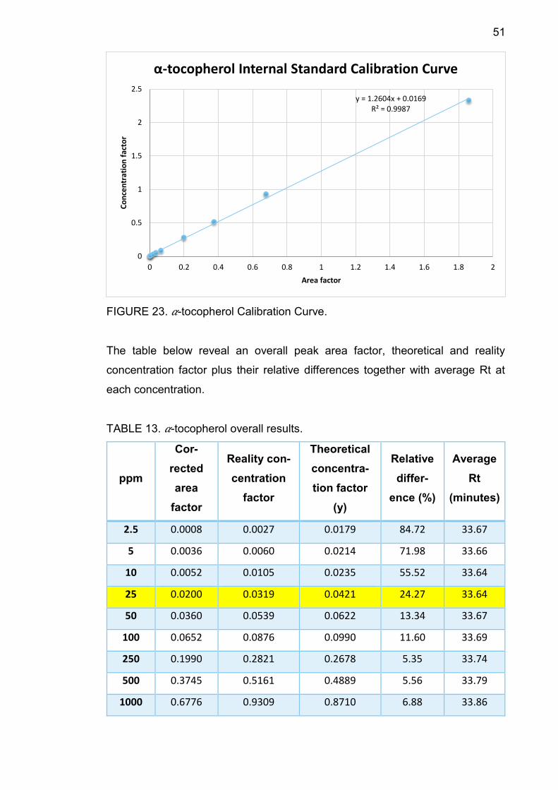
FIGURE 23. 𝛼-tocopherol Calibration Curve.
The table below reveal an overall peak area factor, theoretical and reality
concentration factor plus their relative differences together with average Rt at
each concentration.
TABLE 13. 𝛼-tocopherol overall results.
ppm
Cor-
rected
area
factor
Reality con-
centration
factor
Theoretical
concentra-
tion factor
(y)
Relative
differ-
ence (%)
Average
Rt
(minutes)
2.5 0.0008 0.0027 0.0179 84.72 33.67
5 0.0036 0.0060 0.0214 71.98 33.66
10 0.0052 0.0105 0.0235 55.52 33.64
25 0.0200 0.0319 0.0421 24.27 33.64
50 0.0360 0.0539 0.0622 13.34 33.67
100 0.0652 0.0876 0.0990 11.60 33.69
250 0.1990 0.2821 0.2678 5.35 33.74
500 0.3745 0.5161 0.4889 5.56 33.79
1000 0.6776 0.9309 0.8710 6.88 33.86
y = 1.2604x + 0.0169R² = 0.9987
0
0.5
1
1.5
2
2.5
0 0.2 0.4 0.6 0.8 1 1.2 1.4 1.6 1.8 2
Co
nce
ntr
atio
n f
acto
r
Area factor
α-tocopherol Internal Standard Calibration Curve
52
2500 1.8600 2.3332 2.3612 1.19 33.98
TABLE 13 shows that average Rt increased from 33.64 minutes to 33.98 minutes
along with concentration. At 25 ppm, the relative difference between theoretical
concentration factor and the reality one is 24.27%, smaller than 30%, therefore
25 ppm is the component LOQ.
4.11 DL-𝛼-palmitin
The results show that DL-𝛼-palmitin has:
Average Rt: 23.53.
LOD: 25 ppm.
LOQ: 50 ppm.
Average Response Factor: 3.2189.
Following concentrations of DL-𝛼-palmitin were being analysed: 2.5 ppm, 5 ppm,
10 ppm, 25 ppm, 50 ppm, 100 ppm, 250 ppm, 500 ppm, 1000 ppm and 2500
ppm. Based on the chromatograms that GC-FID generated, the peaks were un-
detectable at the first three concentration. There were symmetrical shapes from
25 ppm to 250 ppm, the peaks started to show fronting at 500 ppm.
A 7 points calibration curve with its equation and R2 was constructed using given
results.
53
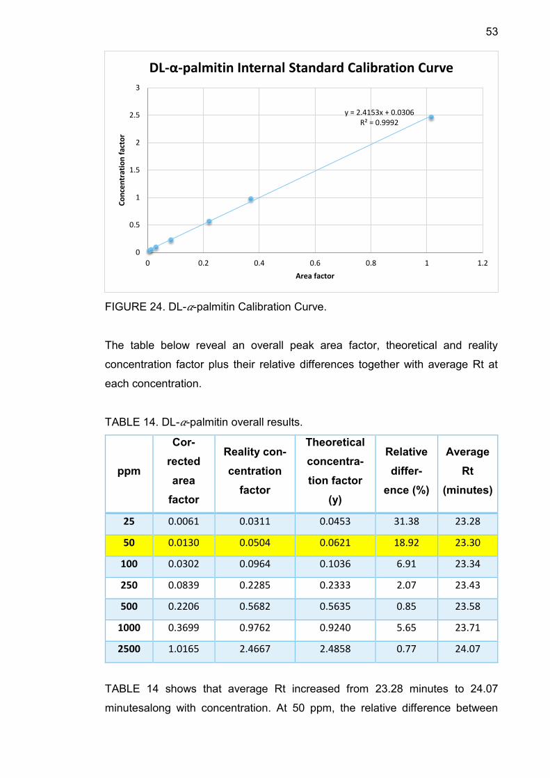
FIGURE 24. DL-𝛼-palmitin Calibration Curve.
The table below reveal an overall peak area factor, theoretical and reality
concentration factor plus their relative differences together with average Rt at
each concentration.
TABLE 14. DL-𝛼-palmitin overall results.
ppm
Cor-
rected
area
factor
Reality con-
centration
factor
Theoretical
concentra-
tion factor
(y)
Relative
differ-
ence (%)
Average
Rt
(minutes)
25 0.0061 0.0311 0.0453 31.38 23.28
50 0.0130 0.0504 0.0621 18.92 23.30
100 0.0302 0.0964 0.1036 6.91 23.34
250 0.0839 0.2285 0.2333 2.07 23.43
500 0.2206 0.5682 0.5635 0.85 23.58
1000 0.3699 0.9762 0.9240 5.65 23.71
2500 1.0165 2.4667 2.4858 0.77 24.07
TABLE 14 shows that average Rt increased from 23.28 minutes to 24.07
minutesalong with concentration. At 50 ppm, the relative difference between
y = 2.4153x + 0.0306R² = 0.9992
0
0.5
1
1.5
2
2.5
3
0 0.2 0.4 0.6 0.8 1 1.2
Co
nce
ntr
atio
n f
acto
r
Area factor
DL-α-palmitin Internal Standard Calibration Curve
54
theoretical concentration factor and the reality one is 18.92%, smaller than 30%,
therefore 50 ppm is the component LOQ.
4.12 TAGs mixture
Following concentrations of TAGs mixture were being analysed: 2.5 ppm, 5 ppm,
10 ppm, 25 ppm, 50 ppm, 100 ppm, 250 ppm, 500 ppm, 1000 ppm and 2500
ppm. There are 5 TAGs presented: tricaprylin, tricaprin, trilaurin, trimyristin and
tripalmitin; each of which accounted for approximately 20% of the solution.
Hence, each components were being analysed at 0.5 ppm, 1 ppm, 2 ppm, 5 ppm,
10 ppm, 20 ppm, 50 ppm, 100 pmm, 200 ppm and 500 ppm. The average
theoretical RF of 5 TAGs is 1.90182.
4.12.1 Tricaprylin
Tricaprylin was the first detected TAG in the mixture. Its results are:
Average Rt: 32.14 minutes.
LOD ≤ 0.5 ppm.
LOQ: 10 ppm.
Average Response Factor: 1.5469.
Based on the chromatograms that GC-FID generated, there were symmetrical
shapes from 0.5 ppm to 50 ppm, the peaks started to show fronting at 100 ppm.
A 10 points calibration curve with its equation and R2 was constructed using given
results.
55
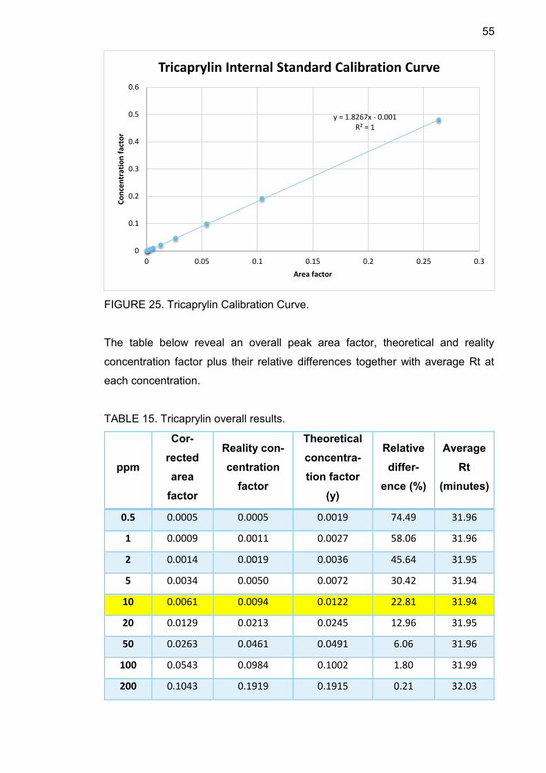
FIGURE 25. Tricaprylin Calibration Curve.
The table below reveal an overall peak area factor, theoretical and reality
concentration factor plus their relative differences together with average Rt at
each concentration.
TABLE 15. Tricaprylin overall results.
ppm
Cor-
rected
area
factor
Reality con-
centration
factor
Theoretical
concentra-
tion factor
(y)
Relative
differ-
ence (%)
Average
Rt
(minutes)
0.5 0.0005 0.0005 0.0019 74.49 31.96
1 0.0009 0.0011 0.0027 58.06 31.96
2 0.0014 0.0019 0.0036 45.64 31.95
5 0.0034 0.0050 0.0072 30.42 31.94
10 0.0061 0.0094 0.0122 22.81 31.94
20 0.0129 0.0213 0.0245 12.96 31.95
50 0.0263 0.0461 0.0491 6.06 31.96
100 0.0543 0.0984 0.1002 1.80 31.99
200 0.1043 0.1919 0.1915 0.21 32.03
y = 1.8267x - 0.001R² = 1
0
0.1
0.2
0.3
0.4
0.5
0.6
0 0.05 0.1 0.15 0.2 0.25 0.3
Co
nce
ntr
atio
n f
acto
r
Area factor
Tricaprylin Internal Standard Calibration Curve
56
500 0.2637 0.4798 0.4827 0.58 33.71
TABLE 15 shows that average Rt increased from 31.94 minutes to 33.71 minutes
along with concentration. At 10 ppm, the relative difference between theoretical
concentration factor and the reality one is 22.81%, smaller than 30%, therefore
10 ppm is the component LOQ.
4.12.2 Tricaprin
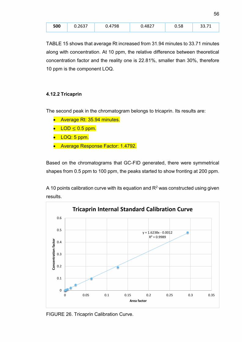
The second peak in the chromatogram belongs to tricaprin. Its results are:
Average Rt: 35.94 minutes.
LOD ≤ 0.5 ppm.
LOQ: 5 ppm.
Average Response Factor: 1.4792.
Based on the chromatograms that GC-FID generated, there were symmetrical
shapes from 0.5 ppm to 100 ppm, the peaks started to show fronting at 200 ppm.
A 10 points calibration curve with its equation and R2 was constructed using given
results.
FIGURE 26. Tricaprin Calibration Curve.
y = 1.6238x - 0.0012R² = 0.9989
0
0.1
0.2
0.3
0.4
0.5
0.6
0 0.05 0.1 0.15 0.2 0.25 0.3 0.35
Co
nce
ntr
atio
n f
acto
r
Area factor
Tricaprin Internal Standard Calibration Curve
57
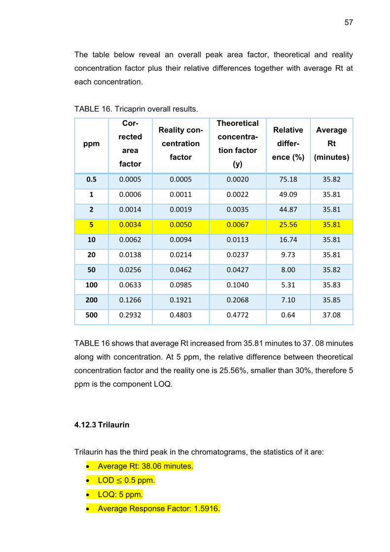
The table below reveal an overall peak area factor, theoretical and reality
concentration factor plus their relative differences together with average Rt at
each concentration.
TABLE 16. Tricaprin overall results.
ppm
Cor-
rected
area
factor
Reality con-
centration
factor
Theoretical
concentra-
tion factor
(y)
Relative
differ-
ence (%)
Average
Rt
(minutes)
0.5 0.0005 0.0005 0.0020 75.18 35.82
1 0.0006 0.0011 0.0022 49.09 35.81
2 0.0014 0.0019 0.0035 44.87 35.81
5 0.0034 0.0050 0.0067 25.56 35.81
10 0.0062 0.0094 0.0113 16.74 35.81
20 0.0138 0.0214 0.0237 9.73 35.81
50 0.0256 0.0462 0.0427 8.00 35.82
100 0.0633 0.0985 0.1040 5.31 35.83
200 0.1266 0.1921 0.2068 7.10 35.85
500 0.2932 0.4803 0.4772 0.64 37.08
TABLE 16 shows that average Rt increased from 35.81 minutes to 37. 08 minutes
along with concentration. At 5 ppm, the relative difference between theoretical
concentration factor and the reality one is 25.56%, smaller than 30%, therefore 5
ppm is the component LOQ.
4.12.3 Trilaurin
Trilaurin has the third peak in the chromatograms, the statistics of it are:
Average Rt: 38.06 minutes.
LOD ≤ 0.5 ppm.
LOQ: 5 ppm.
Average Response Factor: 1.5916.
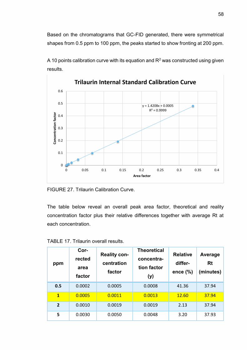
58
Based on the chromatograms that GC-FID generated, there were symmetrical
shapes from 0.5 ppm to 100 ppm, the peaks started to show fronting at 200 ppm.
A 10 points calibration curve with its equation and R2 was constructed using given
results.
FIGURE 27. Trilaurin Calibration Curve.
The table below reveal an overall peak area factor, theoretical and reality
concentration factor plus their relative differences together with average Rt at
each concentration.
TABLE 17. Trilaurin overall results.
ppm
Cor-
rected
area
factor
Reality con-
centration
factor
Theoretical
concentra-
tion factor
(y)
Relative
differ-
ence (%)
Average
Rt
(minutes)
0.5 0.0002 0.0005 0.0008 41.36 37.94
1 0.0005 0.0011 0.0013 12.60 37.94
2 0.0010 0.0019 0.0019 2.13 37.94
5 0.0030 0.0050 0.0048 3.20 37.93
y = 1.4208x + 0.0005R² = 0.9999
0
0.1
0.2
0.3
0.4
0.5
0.6
0 0.05 0.1 0.15 0.2 0.25 0.3 0.35 0.4
Co
nce
ntr
atio
n f
acto
r
Area factor
Trilaurin Internal Standard Calibration Curve
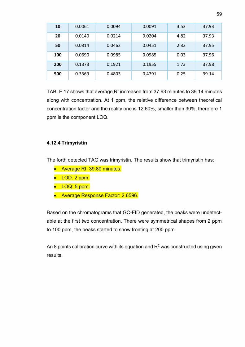
59
10 0.0061 0.0094 0.0091 3.53 37.93
20 0.0140 0.0214 0.0204 4.82 37.93
50 0.0314 0.0462 0.0451 2.32 37.95
100 0.0690 0.0985 0.0985 0.03 37.96
200 0.1373 0.1921 0.1955 1.73 37.98
500 0.3369 0.4803 0.4791 0.25 39.14
TABLE 17 shows that average Rt increased from 37.93 minutes to 39.14 minutes
along with concentration. At 1 ppm, the relative difference between theoretical
concentration factor and the reality one is 12.60%, smaller than 30%, therefore 1
ppm is the component LOQ.
4.12.4 Trimyristin
The forth detected TAG was trimyristin. The results show that trimyristin has:
Average Rt: 39.80 minutes.
LOD: 2 ppm.
LOQ: 5 ppm.
Average Response Factor: 2.6596.
Based on the chromatograms that GC-FID generated, the peaks were undetect-
able at the first two concentration. There were symmetrical shapes from 2 ppm
to 100 ppm, the peaks started to show fronting at 200 ppm.
An 8 points calibration curve with its equation and R2 was constructed using given
results.
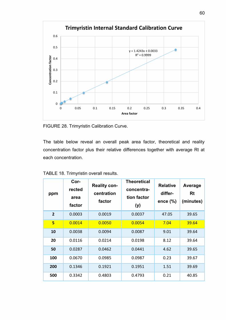
60
FIGURE 28. Trimyristin Calibration Curve.
The table below reveal an overall peak area factor, theoretical and reality
concentration factor plus their relative differences together with average Rt at
each concentration.
TABLE 18. Trimyristin overall results.
ppm
Cor-
rected
area
factor
Reality con-
centration
factor
Theoretical
concentra-
tion factor
(y)
Relative
differ-
ence (%)
Average
Rt
(minutes)
2 0.0003 0.0019 0.0037 47.05 39.65
5 0.0014 0.0050 0.0054 7.04 39.64
10 0.0038 0.0094 0.0087 9.01 39.64
20 0.0116 0.0214 0.0198 8.12 39.64
50 0.0287 0.0462 0.0441 4.62 39.65
100 0.0670 0.0985 0.0987 0.23 39.67
200 0.1346 0.1921 0.1951 1.51 39.69
500 0.3342 0.4803 0.4793 0.21 40.85
y = 1.4243x + 0.0033R² = 0.9999
0
0.1
0.2
0.3
0.4
0.5
0.6
0 0.05 0.1 0.15 0.2 0.25 0.3 0.35 0.4
Co
nce
ntr
atio
n f
acto
r
Area factor
Trimyristin Internal Standard Calibration Curve
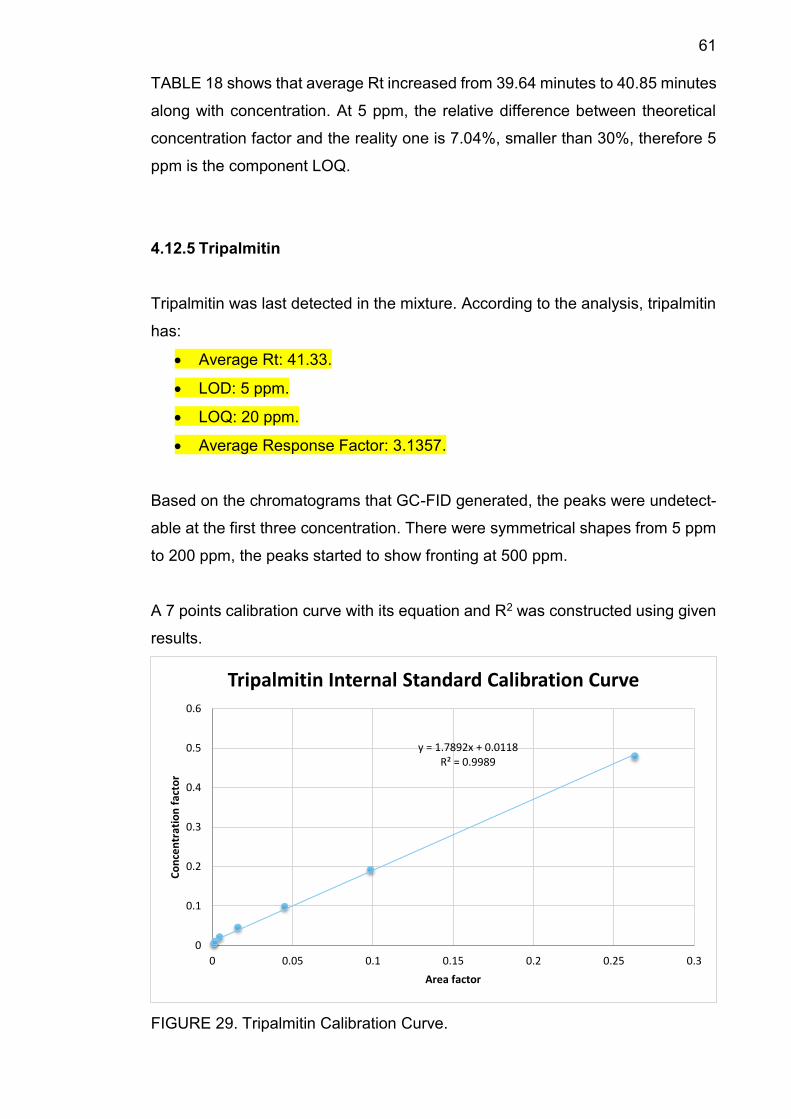
61
TABLE 18 shows that average Rt increased from 39.64 minutes to 40.85 minutes
along with concentration. At 5 ppm, the relative difference between theoretical
concentration factor and the reality one is 7.04%, smaller than 30%, therefore 5
ppm is the component LOQ.
4.12.5 Tripalmitin
Tripalmitin was last detected in the mixture. According to the analysis, tripalmitin
has:
Average Rt: 41.33.
LOD: 5 ppm.
LOQ: 20 ppm.
Average Response Factor: 3.1357.
Based on the chromatograms that GC-FID generated, the peaks were undetect-
able at the first three concentration. There were symmetrical shapes from 5 ppm
to 200 ppm, the peaks started to show fronting at 500 ppm.
A 7 points calibration curve with its equation and R2 was constructed using given
results.
FIGURE 29. Tripalmitin Calibration Curve.
y = 1.7892x + 0.0118R² = 0.9989
0
0.1
0.2
0.3
0.4
0.5
0.6
0 0.05 0.1 0.15 0.2 0.25 0.3
Co
nce
ntr
atio
n f
acto
r
Area factor
Tripalmitin Internal Standard Calibration Curve
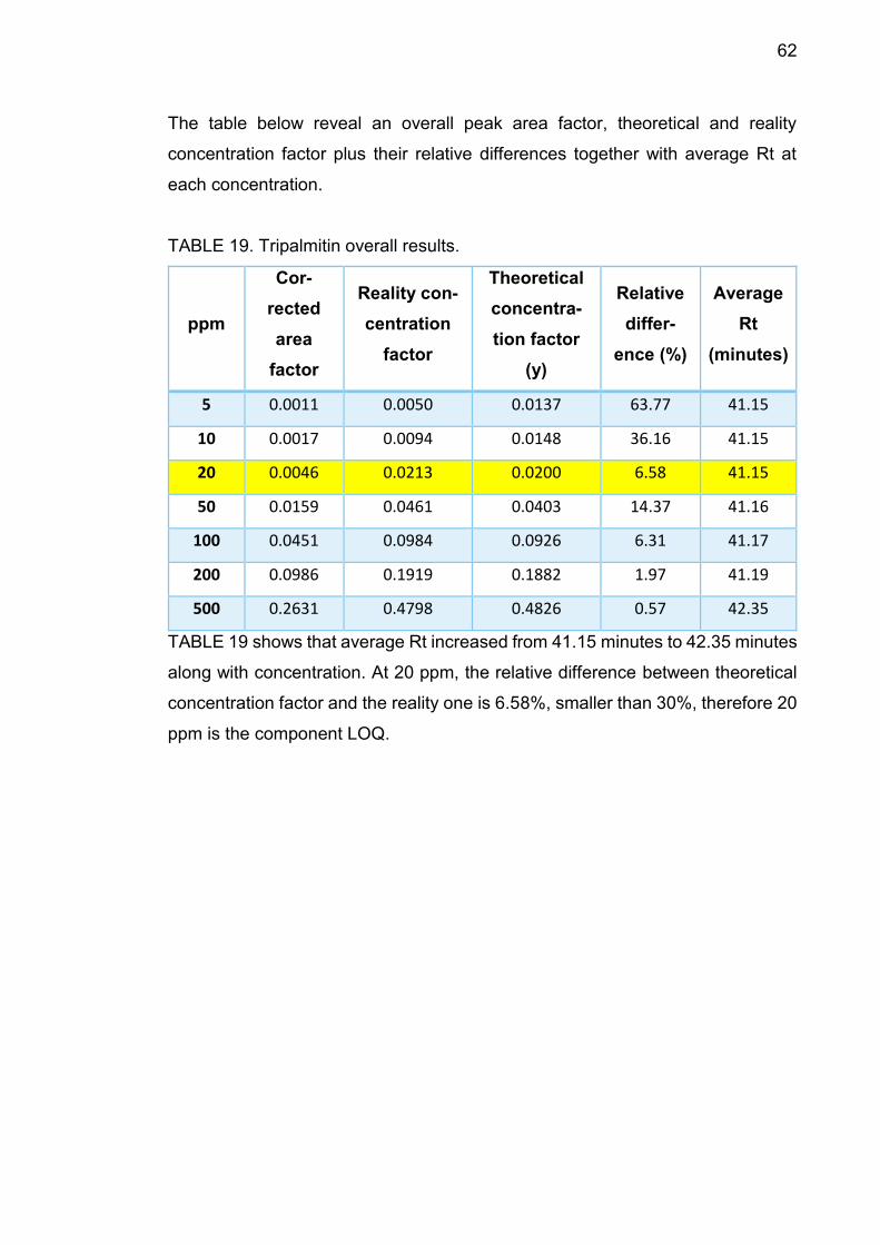
62
The table below reveal an overall peak area factor, theoretical and reality
concentration factor plus their relative differences together with average Rt at
each concentration.
TABLE 19. Tripalmitin overall results.
ppm
Cor-
rected
area
factor
Reality con-
centration
factor
Theoretical
concentra-
tion factor
(y)
Relative
differ-
ence (%)
Average
Rt
(minutes)
5 0.0011 0.0050 0.0137 63.77 41.15
10 0.0017 0.0094 0.0148 36.16 41.15
20 0.0046 0.0213 0.0200 6.58 41.15
50 0.0159 0.0461 0.0403 14.37 41.16
100 0.0451 0.0984 0.0926 6.31 41.17
200 0.0986 0.1919 0.1882 1.97 41.19
500 0.2631 0.4798 0.4826 0.57 42.35
TABLE 19 shows that average Rt increased from 41.15 minutes to 42.35 minutes
along with concentration. At 20 ppm, the relative difference between theoretical
concentration factor and the reality one is 6.58%, smaller than 30%, therefore 20
ppm is the component LOQ.
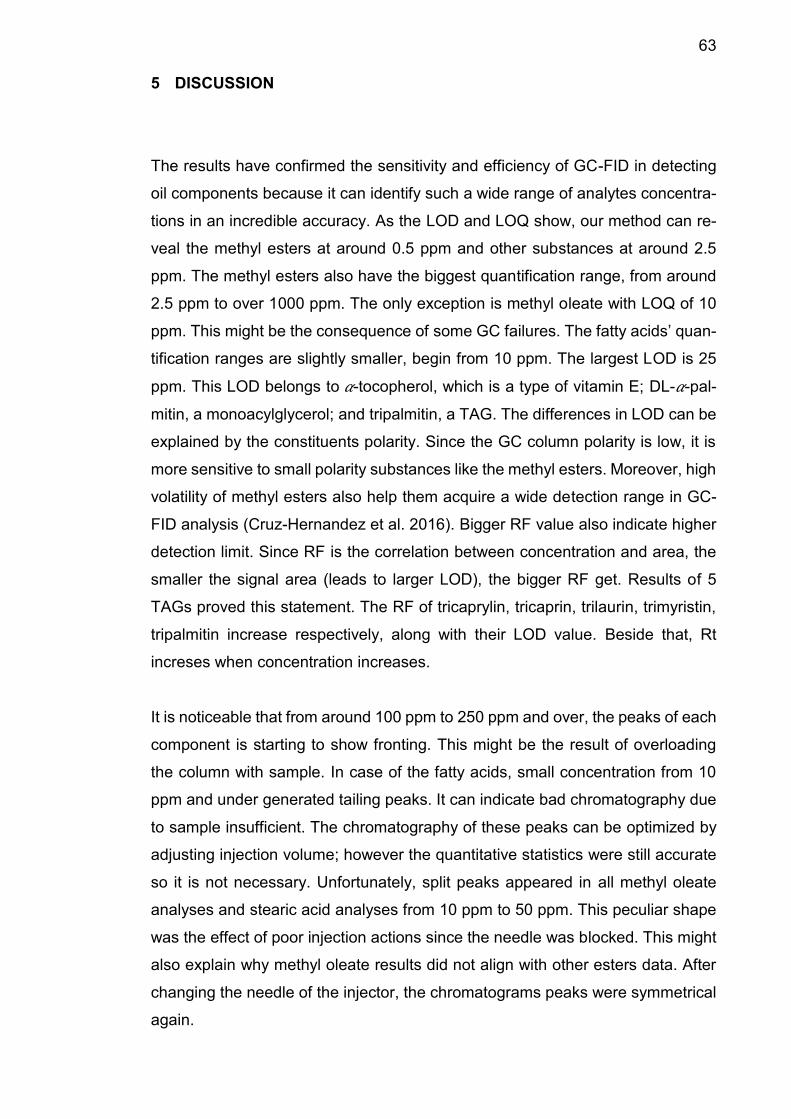
63
5 DISCUSSION
The results have confirmed the sensitivity and efficiency of GC-FID in detecting
oil components because it can identify such a wide range of analytes concentra-
tions in an incredible accuracy. As the LOD and LOQ show, our method can re-
veal the methyl esters at around 0.5 ppm and other substances at around 2.5
ppm. The methyl esters also have the biggest quantification range, from around
2.5 ppm to over 1000 ppm. The only exception is methyl oleate with LOQ of 10
ppm. This might be the consequence of some GC failures. The fatty acids’ quan-
tification ranges are slightly smaller, begin from 10 ppm. The largest LOD is 25
ppm. This LOD belongs to 𝛼-tocopherol, which is a type of vitamin E; DL-𝛼-pal-
mitin, a monoacylglycerol; and tripalmitin, a TAG. The differences in LOD can be
explained by the constituents polarity. Since the GC column polarity is low, it is
more sensitive to small polarity substances like the methyl esters. Moreover, high
volatility of methyl esters also help them acquire a wide detection range in GC-
FID analysis (Cruz-Hernandez et al. 2016). Bigger RF value also indicate higher
detection limit. Since RF is the correlation between concentration and area, the
smaller the signal area (leads to larger LOD), the bigger RF get. Results of 5
TAGs proved this statement. The RF of tricaprylin, tricaprin, trilaurin, trimyristin,
tripalmitin increase respectively, along with their LOD value. Beside that, Rt
increses when concentration increases.
It is noticeable that from around 100 ppm to 250 ppm and over, the peaks of each
component is starting to show fronting. This might be the result of overloading
the column with sample. In case of the fatty acids, small concentration from 10
ppm and under generated tailing peaks. It can indicate bad chromatography due
to sample insufficient. The chromatography of these peaks can be optimized by
adjusting injection volume; however the quantitative statistics were still accurate
so it is not necessary. Unfortunately, split peaks appeared in all methyl oleate
analyses and stearic acid analyses from 10 ppm to 50 ppm. This peculiar shape
was the effect of poor injection actions since the needle was blocked. This might
also explain why methyl oleate results did not align with other esters data. After
changing the needle of the injector, the chromatograms peaks were symmetrical
again.
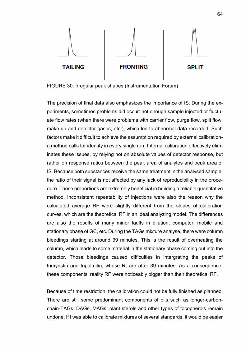
64
FIGURE 30. Irregular peak shapes (Instrumentation Forum)
The precision of final data also emphasizes the importance of IS. During the ex-
periments, sometimes problems did occur: not enough sample injected or fluctu-
ate flow rates (when there were problems with carrier flow, purge flow, split flow,
make-up and detector gases, etc.), which led to abnormal data recorded. Such
factors make it difficult to achieve the assumption required by external calibration-
a method calls for identity in every single run. Internal calibration effectively elim-
inates these issues, by relying not on absolute values of detector response, but
rather on response ratios between the peak area of analytes and peak area of
IS. Because both substances receive the same treatment in the analysed sample,
the ratio of their signal is not affected by any lack of reproducibility in the proce-
dure. These proportions are extremely beneficial in building a reliable quantitative
method. Inconsistent repeatability of injections were also the reason why the
calculated average RF were slightly different from the slopes of calibration
curves, which are the theoretical RF in an ideal analyzing model. The differences
are also the results of many minor faults in dilution, computer, mobile and
stationary phase of GC, etc. During the TAGs mixture analyse, there were column
bleedings starting at around 39 minutes. This is the result of overheating the
column, which leads to some material in the stationary phase coming out into the
detector. Those bleedings caused difficulties in intergrating the peaks of
trimyristin and tripalmitin, whose Rt are after 39 minutes. As a consequence,
these components’ reality RF were noticeably bigger than their theoretical RF.
Because of time restriction, the calibration could not be fully finished as planned.
There are still some predominant components of oils such as longer-carbon-
chain-TAGs, DAGs, MAGs, plant sterols and other types of tocopherols remain
undone. If I was able to calibrate mixtures of several standards, it would be easier

65
to identify them separately in the chromatograms. Nevertheless, the final out-
comes are valuable contributions to the progress of ExtReMo project.
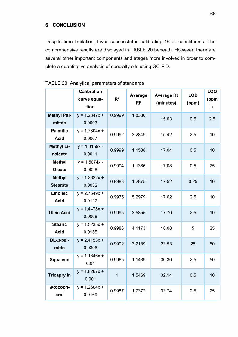
66
6 CONCLUSION
Despite time limitation, I was successful in calibrating 16 oil constituents. The
comprehensive results are displayed in TABLE 20 beneath. However, there are
several other important components and stages more involved in order to com-
plete a quantitative analysis of specialty oils using GC-FID.
TABLE 20. Analytical parameters of standards
Calibration
curve equa-
tion
R2 Average
RF
Average Rt
(minutes)
LOD
(ppm)
LOQ
(ppm
)
Methyl Pal-
mitate
y = 1.2847x +
0.0003
0.9999
1.8380
15.03 0.5 2.5
Palmitic
Acid
y = 1.7804x +
0.0067 0.9992 3.2849 15.42 2.5 10
Methyl Li-
noleate
y = 1.3159x -
0.0011 0.9999 1.1588 17.04 0.5 10
Methyl
Oleate
y = 1.5074x -
0.0028 0.9994 1.1366 17.08 0.5 25
Methyl
Stearate
y = 1.2622x +
0.0032 0.9983 1.2875 17.52 0.25 10
Linoleic
Acid
y = 2.7649x +
0.0117 0.9975 5.2979 17.62 2.5 10
Oleic Acid y = 1.4478x +
0.0068 0.9995 3.5855 17.70 2.5 10
Stearic
Acid
y = 1.5235x +
0.0155 0.9986 4.1173 18.08 5 25
DL-𝛼-pal-
mitin
y = 2.4153x +
0.0306 0.9992 3.2189 23.53 25 50
Squalene y = 1.1646x +
0.01 0.9965 1.1439 30.30 2.5 50
Tricaprylin y = 1.8267x +
0.001 1 1.5469 32.14 0.5 10
𝛼-tocoph-
erol
y = 1.2604x +
0.0169 0.9987 1.7372 33.74 2.5 25
67
Tricaprin y = 1.6238x +
0.0012 0.9989 1.4792 35.94 0.5 5
Trilaurin y = 1.4208x + 0.0005
0.9999 1.5916 38.06 0.5 1
Trimyristin y = 1.4243x + 0.0033
0.9999 2.6596 39.80 2 5
Tripalmitin y = 1.7892x + 0.0118
0.9989 3.1357 41.33 5 20
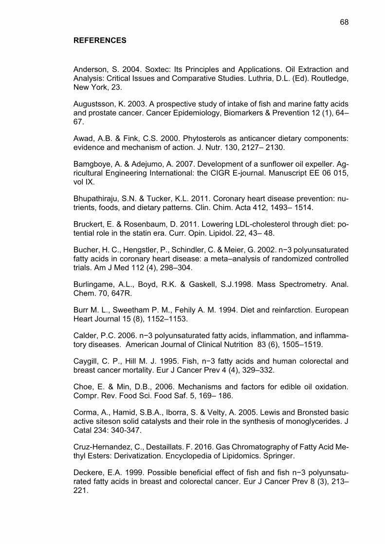
68
REFERENCES
Anderson, S. 2004. Soxtec: Its Principles and Applications. Oil Extraction and Analysis: Critical Issues and Comparative Studies. Luthria, D.L. (Ed). Routledge, New York, 23.
Augustsson, K. 2003. A prospective study of intake of fish and marine fatty acids and prostate cancer. Cancer Epidemiology, Biomarkers & Prevention 12 (1), 64–67.
Awad, A.B. & Fink, C.S. 2000. Phytosterols as anticancer dietary components: evidence and mechanism of action. J. Nutr. 130, 2127– 2130.
Bamgboye, A. & Adejumo, A. 2007. Development of a sunflower oil expeller. Ag-ricultural Engineering International: the CIGR E-journal. Manuscript EE 06 015, vol IX.
Bhupathiraju, S.N. & Tucker, K.L. 2011. Coronary heart disease prevention: nu-trients, foods, and dietary patterns. Clin. Chim. Acta 412, 1493– 1514.
Bruckert, E. & Rosenbaum, D. 2011. Lowering LDL-cholesterol through diet: po-tential role in the statin era. Curr. Opin. Lipidol. 22, 43– 48.
Bucher, H. C., Hengstler, P., Schindler, C. & Meier, G. 2002. n−3 polyunsaturated fatty acids in coronary heart disease: a meta–analysis of randomized controlled trials. Am J Med 112 (4), 298–304.
Burlingame, A.L., Boyd, R.K. & Gaskell, S.J.1998. Mass Spectrometry. Anal. Chem. 70, 647R.
Burr M. L., Sweetham P. M., Fehily A. M. 1994. Diet and reinfarction. European Heart Journal 15 (8), 1152–1153.
Calder, P.C. 2006. n−3 polyunsaturated fatty acids, inflammation, and inflamma-tory diseases. American Journal of Clinical Nutrition 83 (6), 1505–1519.
Caygill, C. P., Hill M. J. 1995. Fish, n−3 fatty acids and human colorectal and breast cancer mortality. Eur J Cancer Prev 4 (4), 329–332.
Choe, E. & Min, D.B., 2006. Mechanisms and factors for edible oil oxidation. Compr. Rev. Food Sci. Food Saf. 5, 169– 186.
Corma, A., Hamid, S.B.A., Iborra, S. & Velty, A. 2005. Lewis and Bronsted basic active siteson solid catalysts and their role in the synthesis of monoglycerides. J Catal 234: 340-347.
Cruz-Hernandez, C., Destaillats. F. 2016. Gas Chromatography of Fatty Acid Me-thyl Esters: Derivatization. Encyclopedia of Lipidomics. Springer.
Deckere, E.A. 1999. Possible beneficial effect of fish and fish n−3 polyunsatu-rated fatty acids in breast and colorectal cancer. Eur J Cancer Prev 8 (3), 213–221.
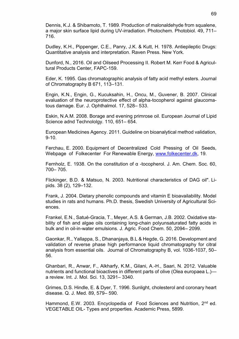
69
Dennis, K.J. & Shibamoto, T. 1989. Production of malonaldehyde from squalene, a major skin surface lipid during UV-irradiation. Photochem. Photobiol. 49, 711– 716.
Dudley, K.H., Pippenger, C.E., Panry, J.K. & Kutt, H. 1978. Antiepileptic Drugs: Quantitative analysis and interpretation. Raven Press. New York.
Dunford, N., 2016. Oil and Oilseed Processing II. Robert M. Kerr Food & Agricul-tural Products Center, FAPC-159.
Eder, K. 1995. Gas chromatographic analysis of fatty acid methyl esters. Journal of Chromatography B 671, 113–131.
Engin, K.N., Engin, G., Kucuksahin, H., Oncu, M., Guvener, B. 2007. Clinical evaluation of the neuroprotective effect of alpha-tocopherol against glaucoma-tous damage. Eur. J. Ophthalmol. 17, 528– 533.
Eskin, N.A.M. 2008. Borage and evening primrose oil. European Journal of Lipid Science adnd Technololgy. 110, 651– 654.
European Medicines Agency. 2011. Guideline on bioanalytical method validation, 9-10.
Ferchau, E. 2000. Equipment of Decentralized Cold Pressing of Oil Seeds, Webpage of Folkecenter For Renewable Energy, www.folkecenter.dk, 19.
Fernholz, E. 1938. On the constitution of α -tocopherol. J. Am. Chem. Soc. 60, 700– 705.
Flickinger, B.D. & Matsuo, N. 2003. Nutritional characteristics of DAG oil". Li-pids. 38 (2), 129–132.
Frank, J. 2004. Dietary phenolic compounds and vitamin E bioavailability. Model studies in rats and humans. Ph.D. thesis, Swedish University of Agricultural Sci-ences.
Frankel, E.N., Satué-Gracia, T., Meyer, A.S. & German, J.B. 2002. Oxidative sta-bility of fish and algae oils containing long-chain polyunsaturated fatty acids in bulk and in oil-in-water emulsions. J. Agric. Food Chem. 50, 2094– 2099.
Gaonkar, R., Yallappa, S., Dhananjaya, B.L & Hegde, G. 2016. Development and validation of reverse phase high performance liquid chromatography for citral analysis from essential oils. Journal of Chromatography B, vol. 1036-1037, 50–56.
Ghanbari, R., Anwar, F., Alkharfy, K.M., Gilani, A.-H., Saari, N. 2012. Valuable nutrients and functional bioactives in different parts of olive (Olea europaea L.)—a review. Int. J. Mol. Sci. 13, 3291– 3340.
Grimes, D.S. Hindle, E. & Dyer, T. 1996. Sunlight, cholesterol and coronary heart disease. Q. J. Med. 89, 579– 590.
Hammond, E.W. 2003. Encyclopedia of Food Sciences and Nutrition, 2nd ed. VEGETABLE OIL- Types and properties. Academic Press, 5899.
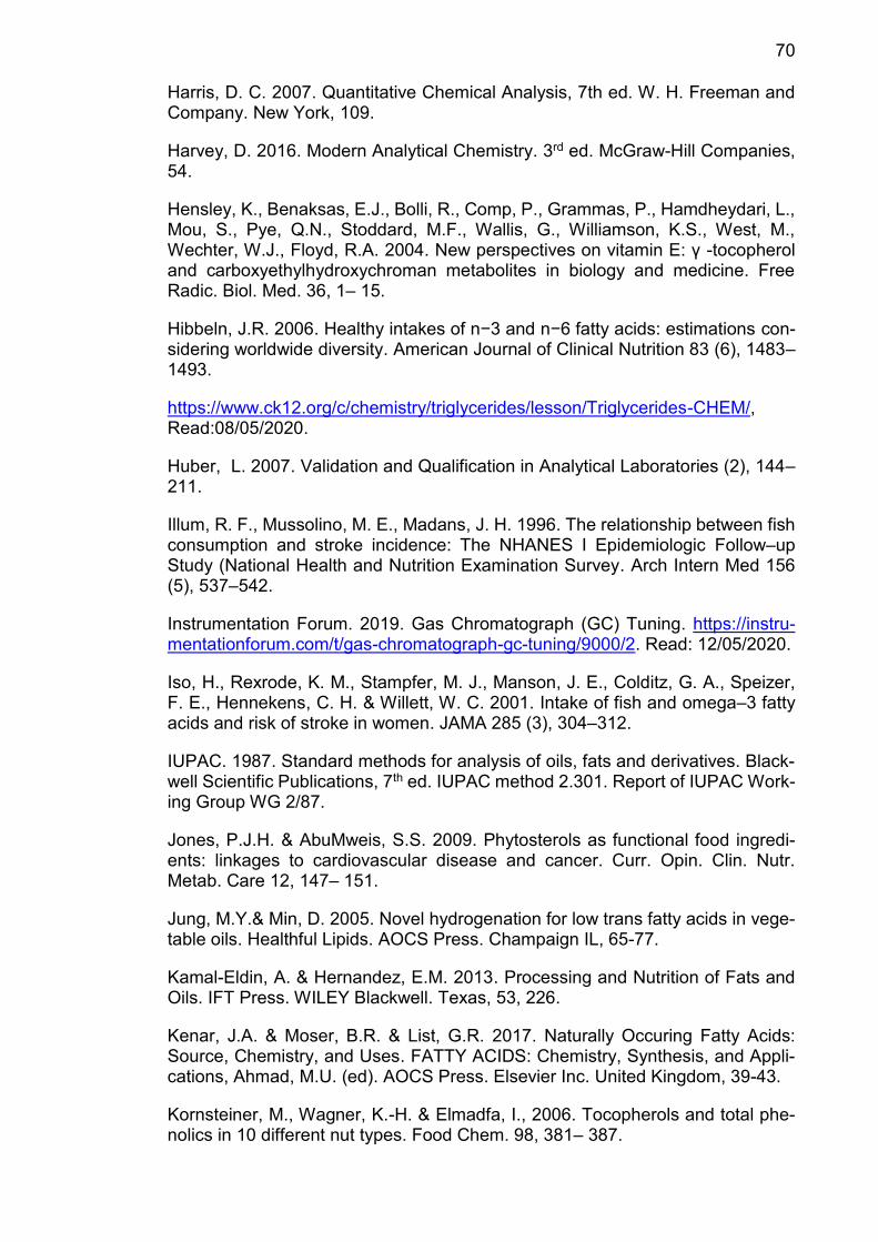
70
Harris, D. C. 2007. Quantitative Chemical Analysis, 7th ed. W. H. Freeman and Company. New York, 109.
Harvey, D. 2016. Modern Analytical Chemistry. 3rd ed. McGraw-Hill Companies, 54.
Hensley, K., Benaksas, E.J., Bolli, R., Comp, P., Grammas, P., Hamdheydari, L., Mou, S., Pye, Q.N., Stoddard, M.F., Wallis, G., Williamson, K.S., West, M., Wechter, W.J., Floyd, R.A. 2004. New perspectives on vitamin E: γ -tocopherol and carboxyethylhydroxychroman metabolites in biology and medicine. Free Radic. Biol. Med. 36, 1– 15.
Hibbeln, J.R. 2006. Healthy intakes of n−3 and n−6 fatty acids: estimations con-sidering worldwide diversity. American Journal of Clinical Nutrition 83 (6), 1483–1493.
https://www.ck12.org/c/chemistry/triglycerides/lesson/Triglycerides-CHEM/, Read:08/05/2020.
Huber, L. 2007. Validation and Qualification in Analytical Laboratories (2), 144–211.
Illum, R. F., Mussolino, M. E., Madans, J. H. 1996. The relationship between fish consumption and stroke incidence: The NHANES I Epidemiologic Follow–up Study (National Health and Nutrition Examination Survey. Arch Intern Med 156 (5), 537–542.
Instrumentation Forum. 2019. Gas Chromatograph (GC) Tuning. https://instru-mentationforum.com/t/gas-chromatograph-gc-tuning/9000/2. Read: 12/05/2020.
Iso, H., Rexrode, K. M., Stampfer, M. J., Manson, J. E., Colditz, G. A., Speizer, F. E., Hennekens, C. H. & Willett, W. C. 2001. Intake of fish and omega–3 fatty acids and risk of stroke in women. JAMA 285 (3), 304–312.
IUPAC. 1987. Standard methods for analysis of oils, fats and derivatives. Black-well Scientific Publications, 7th ed. IUPAC method 2.301. Report of IUPAC Work-ing Group WG 2/87.
Jones, P.J.H. & AbuMweis, S.S. 2009. Phytosterols as functional food ingredi-ents: linkages to cardiovascular disease and cancer. Curr. Opin. Clin. Nutr. Metab. Care 12, 147– 151.
Jung, M.Y.& Min, D. 2005. Novel hydrogenation for low trans fatty acids in vege-table oils. Healthful Lipids. AOCS Press. Champaign IL, 65-77.
Kamal-Eldin, A. & Hernandez, E.M. 2013. Processing and Nutrition of Fats and Oils. IFT Press. WILEY Blackwell. Texas, 53, 226.
Kenar, J.A. & Moser, B.R. & List, G.R. 2017. Naturally Occuring Fatty Acids: Source, Chemistry, and Uses. FATTY ACIDS: Chemistry, Synthesis, and Appli-cations, Ahmad, M.U. (ed). AOCS Press. Elsevier Inc. United Kingdom, 39-43.
Kornsteiner, M., Wagner, K.-H. & Elmadfa, I., 2006. Tocopherols and total phe-nolics in 10 different nut types. Food Chem. 98, 381– 387.
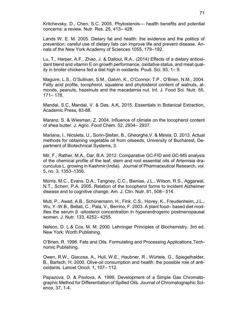
71
Kritchevsky, D., Chen, S.C. 2005. Phytosterols— health benefits and potential concerns: a review. Nutr. Res. 25, 413– 428.
Lands W. E. M. 2005. Dietary fat and health: the evidence and the politics of prevention: careful use of dietary fats can improve life and prevent disease. An-nals of the New York Academy of Sciences 1055, 179–192.
Lu, T., Harper, A.F., Zhao, J. & Dalloul, R.A., (2014) Effects of a dietary antioxi-dant blend and vitamin E on growth performance, oxidative status, and meat qual-ity in broiler chickens fed a diet high in oxidants. Poult. Sci. 93, 1– 9.
Maguire, L.S., O’Sullivan, S.M., Galvin, K., O’Connor, T.P., O’Brien, N.M., 2004. Fatty acid profile, tocopherol, squalene and phytosterol content of walnuts, al-monds, peanuts, hazelnuts and the macadamia nut. Int. J. Food Sci. Nutr. 55, 171– 178.
Mandal, S.C, Mandal, V. & Das, A.K. 2015. Essentials in Botanical Extraction, Academic Press, 83-88.
Maranz, S. & Wiesman, Z. 2004. Influence of climate on the tocopherol content of shea butter. J. Agric. Food Chem. 52, 2934– 2937.
Mariana, I., Nicoleta, U., Sorin-Ştefan, B., Gheorghe,V. & Mirela, D. 2013. Actual methods for obtaining vegetable oil from oilseeds, University of Bucharest, De-partment of Biotechnical Systems, 3.
Mir, F., Rather, M.A., Dar, B.A. 2012. Comparative GC-FID and GC-MS analysis of the chemical profile of the leaf, stem and root essential oils of Artemisia dra-cunculus L. growing in Kashmir (India). Journal of Pharmaceutical Research, vol. 5, no. 3, 1353–1356.
Morris, M.C., Evans, D.A., Tangney, C.C., Bienias, J.L., Wilson, R.S., Aggarwal, N.T., Scherr, P.A. 2005. Relation of the tocopherol forms to incident Alzheimer disease and to cognitive change. Am. J. Clin. Nutr. 81, 508– 514.
Muti, P., Awad, A.B., Schünemann, H., Fink, C.S., Hovey, K., Freudenheim, J.L., Wu, Y.-W.B., Bellati, C., Pala, V., Berrino, F. 2003. A plant food– based diet mod-ifies the serum β -sitosterol concentration in hyperandrogenic postmenopausal women. J. Nutr. 133, 4252– 4255.
Nelson, D. L.& Cox, M. M. 2000. Lehninger Principles of Biochemistry. 3rd ed. New York: Worth Publishing.
O’Brien, R. 1998. Fats and Oils. Formulating and Processing Applications.Tech-nomic Publishing.
Owen, R.W., Giacosa, A., Hull, W.E., Haubner, R., Würtele, G., Spiegelhalder, B., Bartsch, H. 2000. Olive-oil consumption and health: the possible role of anti-oxidants. Lancet Oncol. 1, 107– 112.
Papazova, D. & Pavlova, A. 1999. Development of a Simple Gas Chromato-graphic Method for Differentiation of Spilled Oils. Journal of Chromatographic Sci-ence, 37, 1-4.
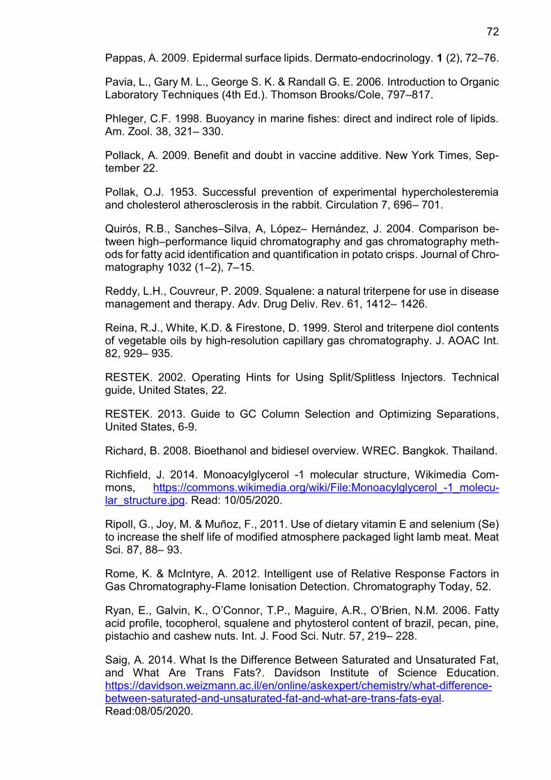
72
Pappas, A. 2009. Epidermal surface lipids. Dermato-endocrinology. 1 (2), 72–76.
Pavia, L., Gary M. L., George S. K. & Randall G. E. 2006. Introduction to Organic Laboratory Techniques (4th Ed.). Thomson Brooks/Cole, 797–817.
Phleger, C.F. 1998. Buoyancy in marine fishes: direct and indirect role of lipids. Am. Zool. 38, 321– 330.
Pollack, A. 2009. Benefit and doubt in vaccine additive. New York Times, Sep-tember 22.
Pollak, O.J. 1953. Successful prevention of experimental hypercholesteremia and cholesterol atherosclerosis in the rabbit. Circulation 7, 696– 701.
Quiros, R.B., Sanches–Silva, A, Lopez– Hernandez, J. 2004. Comparison be-tween high–performance liquid chromatography and gas chromatography meth-ods for fatty acid identification and quantification in potato crisps. Journal of Chro-matography 1032 (1–2), 7–15.
Reddy, L.H., Couvreur, P. 2009. Squalene: a natural triterpene for use in disease management and therapy. Adv. Drug Deliv. Rev. 61, 1412– 1426.
Reina, R.J., White, K.D. & Firestone, D. 1999. Sterol and triterpene diol contents of vegetable oils by high-resolution capillary gas chromatography. J. AOAC Int. 82, 929– 935.
RESTEK. 2002. Operating Hints for Using Split/Splitless Injectors. Technical guide, United States, 22.
RESTEK. 2013. Guide to GC Column Selection and Optimizing Separations, United States, 6-9.
Richard, B. 2008. Bioethanol and bidiesel overview. WREC. Bangkok. Thailand.
Richfield, J. 2014. Monoacylglycerol -1 molecular structure, Wikimedia Com-mons, https://commons.wikimedia.org/wiki/File:Monoacylglycerol_-1_molecu-lar_structure.jpg. Read: 10/05/2020.
Ripoll, G., Joy, M. & Muñoz, F., 2011. Use of dietary vitamin E and selenium (Se) to increase the shelf life of modified atmosphere packaged light lamb meat. Meat Sci. 87, 88– 93.
Rome, K. & McIntyre, A. 2012. Intelligent use of Relative Response Factors in Gas Chromatography-Flame Ionisation Detection. Chromatography Today, 52.
Ryan, E., Galvin, K., O’Connor, T.P., Maguire, A.R., O’Brien, N.M. 2006. Fatty acid profile, tocopherol, squalene and phytosterol content of brazil, pecan, pine, pistachio and cashew nuts. Int. J. Food Sci. Nutr. 57, 219– 228.
Saig, A. 2014. What Is the Difference Between Saturated and Unsaturated Fat, and What Are Trans Fats?. Davidson Institute of Science Education. https://davidson.weizmann.ac.il/en/online/askexpert/chemistry/what-difference-between-saturated-and-unsaturated-fat-and-what-are-trans-fats-eyal. Read:08/05/2020.
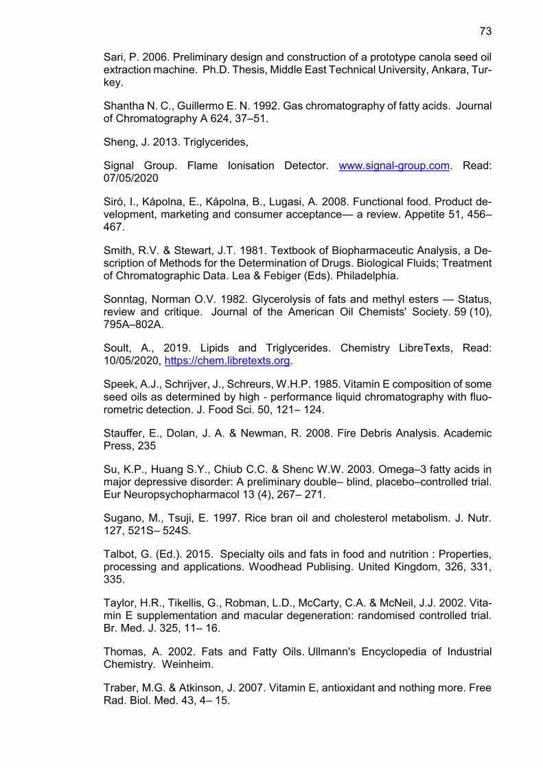
73
Sari, P. 2006. Preliminary design and construction of a prototype canola seed oil extraction machine. Ph.D. Thesis, Middle East Technical University, Ankara, Tur-key.
Shantha N. C., Guillermo E. N. 1992. Gas chromatography of fatty acids. Journal of Chromatography A 624, 37–51.
Sheng, J. 2013. Triglycerides,
Signal Group. Flame Ionisation Detector. www.signal-group.com. Read: 07/05/2020
Siró, I., Kápolna, E., Kápolna, B., Lugasi, A. 2008. Functional food. Product de-velopment, marketing and consumer acceptance— a review. Appetite 51, 456– 467.
Smith, R.V. & Stewart, J.T. 1981. Textbook of Biopharmaceutic Analysis, a De-scription of Methods for the Determination of Drugs. Biological Fluids; Treatment of Chromatographic Data. Lea & Febiger (Eds). Philadelphia.
Sonntag, Norman O.V. 1982. Glycerolysis of fats and methyl esters — Status, review and critique. Journal of the American Oil Chemists' Society. 59 (10), 795A–802A.
Soult, A., 2019. Lipids and Triglycerides. Chemistry LibreTexts, Read: 10/05/2020, https://chem.libretexts.org.
Speek, A.J., Schrijver, J., Schreurs, W.H.P. 1985. Vitamin E composition of some seed oils as determined by high ‐ performance liquid chromatography with fluo-rometric detection. J. Food Sci. 50, 121– 124.
Stauffer, E., Dolan, J. A. & Newman, R. 2008. Fire Debris Analysis. Academic Press, 235
Su, K.P., Huang S.Y., Chiub C.C. & Shenc W.W. 2003. Omega–3 fatty acids in major depressive disorder: A preliminary double– blind, placebo–controlled trial. Eur Neuropsychopharmacol 13 (4), 267– 271.
Sugano, M., Tsuji, E. 1997. Rice bran oil and cholesterol metabolism. J. Nutr. 127, 521S– 524S.
Talbot, G. (Ed.). 2015. Specialty oils and fats in food and nutrition : Properties, processing and applications. Woodhead Publising. United Kingdom, 326, 331, 335.
Taylor, H.R., Tikellis, G., Robman, L.D., McCarty, C.A. & McNeil, J.J. 2002. Vita-min E supplementation and macular degeneration: randomised controlled trial. Br. Med. J. 325, 11– 16.
Thomas, A. 2002. Fats and Fatty Oils. Ullmann's Encyclopedia of Industrial Chemistry. Weinheim.
Traber, M.G. & Atkinson, J. 2007. Vitamin E, antioxidant and nothing more. Free Rad. Biol. Med. 43, 4– 15.

74
Wolosik, K., Knas, M., Zalewska, A., Niczyporuk, M.& Przystupa A.W. 2013. The importance and perspective of plant-based squalene in cosmetology. J Cosmet Sci. 2013 Jan-Feb;64(1), 59-66.
Woyengo, T.A., Ramprasath, V.R. & Jones, P.J.H. 2009. Anticancer effects of phytosterols. Eur. J. Clin. Nutr. 63, 813– 820.
Yang, X. & Boyle, R.A. 2016. Sensory Evaluation of Oils/Fats and Oil/Fat–Based Foods. Oxidative Stability and Shelf Life of Foods Containing Oils and Fats. Hu & Jacobsen (Eds). AOCS Press.
Zheng, Y., Chen, X. & Shen, Y. 2008. Commodity chemicals derived from glyc-erol, an important biorefinery feedstock. Chem Rev 108, 5253-5277.
75
APPENDICES
Appendix 1. Squalene chromatograms signals
ppm
1st injection 2nd injection 3rd injection Concentration
Area IS Area
Std Area IS Area Std Area IS Area Std
IS in vial
(g)
Std in vial
(g)
2.5 1315.181 2.325 1271.055 2.161 1259.872 2.22 0.00102222 4.71237E-07
5 1258.809 4.872 1205.368 4.822 1161.393 4.684 0.00094669 1.31172E-06
10 1145.113 8.504 1146.077 8.596 1156.168 8.792 0.00117038 2.51051E-06
25 1047.255 22.841 1029.003 23.24 1024.812 22.731 0.00132469 5.22834E-06
50 1051.998 43.372 1081.835 43.94 1075.733 43.398 0.00116899 1.03813E-05
100 403.606 29.551 1060.208 87.771 1047.027 85.684 0.00125518 2.49795E-05
250 71.096 5.872 1122.976 194.72 1107.778 192.424 0.00116845 5.44334E-05
500 582.954 201.227 939.983 372.335 475.209 156.843 0.00123186 0.000103221
1000 19.825 11.737 96.308 32.056 920.413 650.898 0.00120507 0.000262626
2500 113.65 68.735 1012.233 1829.464 1138.827 2151.493 0.00124672 0.000498993
Squalene 2500 ppm chromatogram.
76
Appendix 2. Methyl Palmitate chromatograms signals
ppm
1st injection 2nd injection 3rd injection Concentration
Area IS Area
Std Area IS
Area
Std Area IS
Area
Std
IS in vial
(g)
Std in vial
(g)
0.5 943.401 0.468 936.895 0.465 929.722 0.467 0.00102222 4.71237E-07
1 860.732 1.155 879.465 1.124 943.483 1.234 0.00094669 1.31172E-06
2.5 1132.551 1.974 1149.271 2.012 1186.628 2.025 0.00117038 2.51051E-06
5 1299.694 5.22 1184.804 4.811 1332.019 5.458 0.00132469 5.22834E-06
10 1103.631 8.026 1103.955 7.859 1120.934 8.054 0.00116899 1.03813E-05
25 1140.58 19.048 1249.03 21.19 1264.832 20.82 0.00125518 2.49795E-05
50 1224.296 44.323 1150.698 41.538 1182.294 42.082 0.00116845 5.44334E-05
100 1160.989 76.659 1203.905 81.443 1262.498 84.611 0.00123186 0.000103221
250 1185.359 196.71 1200.307 201.534 1199.448 194.482 0.00120507 0.000262626
500 333.352 98.015 1274.718 398.759 1273.551 401.048 0.00124672 0.000498993
1000 982.213 878.887 1129.571 1007.05 1066.034 961.901 0.00105174 0.001208631
Methyl palmitate 1000 ppm chromatogram.
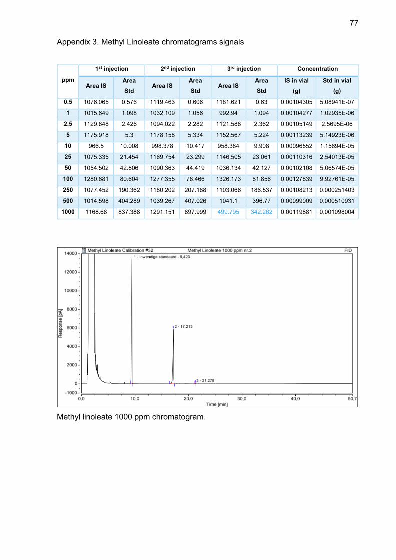
77
Appendix 3. Methyl Linoleate chromatograms signals
ppm
1st injection 2nd injection 3rd injection Concentration
Area IS Area
Std Area IS
Area
Std Area IS
Area
Std
IS in vial
(g)
Std in vial
(g)
0.5 1076.065 0.576 1119.463 0.606 1181.621 0.63 0.00104305 5.08941E-07
1 1015.649 1.098 1032.109 1.056 992.94 1.094 0.00104277 1.02935E-06
2.5 1129.848 2.426 1094.022 2.282 1121.588 2.362 0.00105149 2.5695E-06
5 1175.918 5.3 1178.158 5.334 1152.567 5.224 0.00113239 5.14923E-06
10 966.5 10.008 998.378 10.417 958.384 9.908 0.00096552 1.15894E-05
25 1075.335 21.454 1169.754 23.299 1146.505 23.061 0.00110316 2.54013E-05
50 1054.502 42.806 1090.363 44.419 1036.134 42.127 0.00102108 5.06574E-05
100 1280.681 80.604 1277.355 78.466 1326.173 81.856 0.00127839 9.92761E-05
250 1077.452 190.362 1180.202 207.188 1103.066 186.537 0.00108213 0.000251403
500 1014.598 404.289 1039.267 407.026 1041.1 396.77 0.00099009 0.000510931
1000 1168.68 837.388 1291.151 897.999 499.795 342.262 0.00119881 0.001098004
Methyl linoleate 1000 ppm chromatogram.
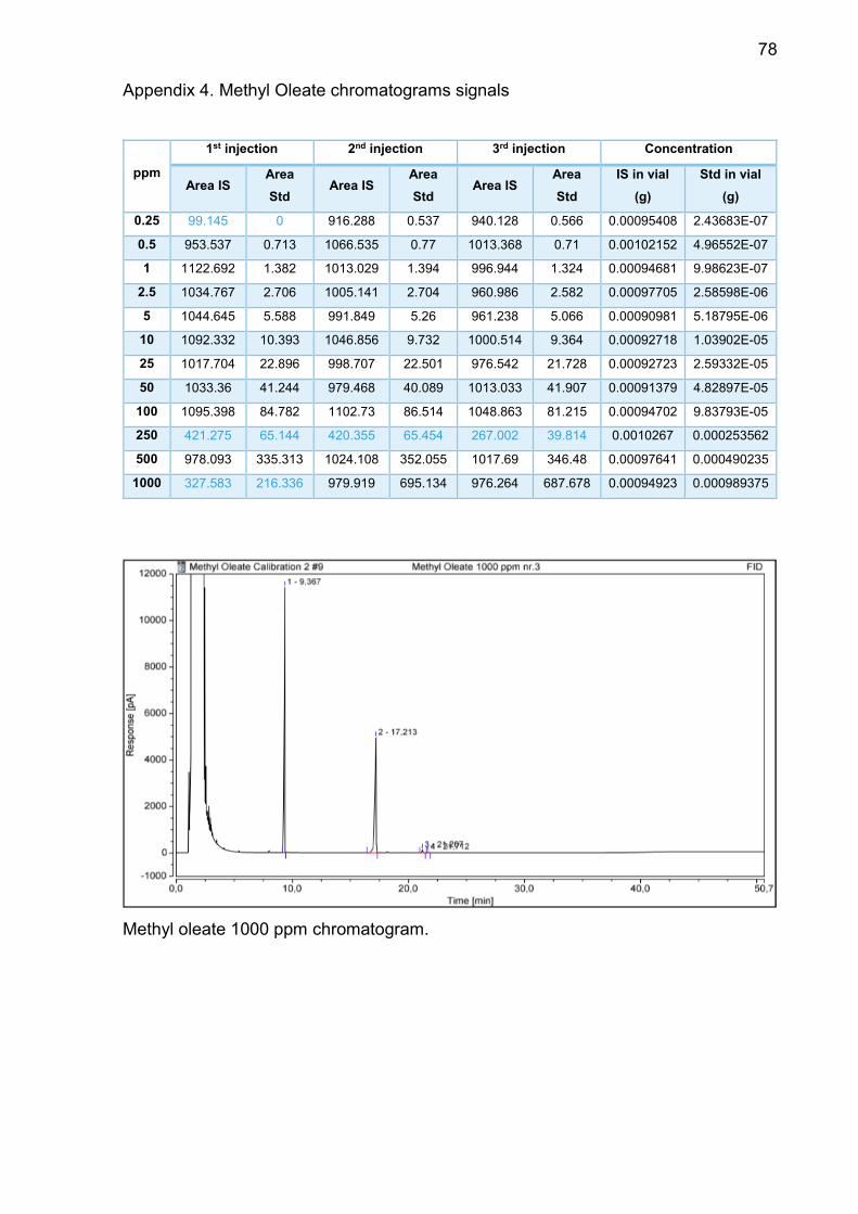
78
Appendix 4. Methyl Oleate chromatograms signals
ppm
1st injection 2nd injection 3rd injection Concentration
Area IS Area
Std Area IS
Area
Std Area IS
Area
Std
IS in vial
(g)
Std in vial
(g)
0.25 99.145 0 916.288 0.537 940.128 0.566 0.00095408 2.43683E-07
0.5 953.537 0.713 1066.535 0.77 1013.368 0.71 0.00102152 4.96552E-07
1 1122.692 1.382 1013.029 1.394 996.944 1.324 0.00094681 9.98623E-07
2.5 1034.767 2.706 1005.141 2.704 960.986 2.582 0.00097705 2.58598E-06
5 1044.645 5.588 991.849 5.26 961.238 5.066 0.00090981 5.18795E-06
10 1092.332 10.393 1046.856 9.732 1000.514 9.364 0.00092718 1.03902E-05
25 1017.704 22.896 998.707 22.501 976.542 21.728 0.00092723 2.59332E-05
50 1033.36 41.244 979.468 40.089 1013.033 41.907 0.00091379 4.82897E-05
100 1095.398 84.782 1102.73 86.514 1048.863 81.215 0.00094702 9.83793E-05
250 421.275 65.144 420.355 65.454 267.002 39.814 0.0010267 0.000253562
500 978.093 335.313 1024.108 352.055 1017.69 346.48 0.00097641 0.000490235
1000 327.583 216.336 979.919 695.134 976.264 687.678 0.00094923 0.000989375
Methyl oleate 1000 ppm chromatogram.
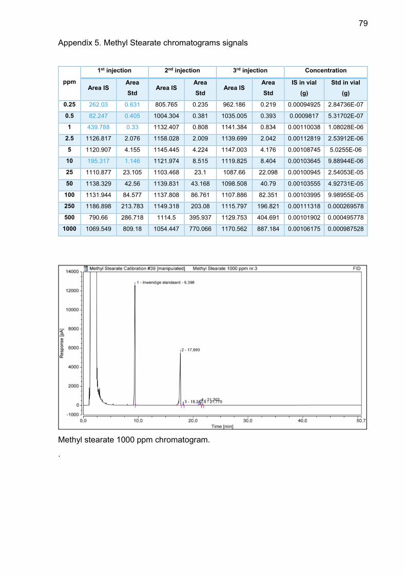
79
Appendix 5. Methyl Stearate chromatograms signals
ppm
1st injection 2nd injection 3rd injection Concentration
Area IS Area
Std Area IS
Area
Std Area IS
Area
Std
IS in vial
(g)
Std in vial
(g)
0.25 262.03 0.631 805.765 0.235 962.186 0.219 0.00094925 2.84736E-07
0.5 82.247 0.405 1004.304 0.381 1035.005 0.393 0.0009817 5.31702E-07
1 439.788 0.33 1132.407 0.808 1141.384 0.834 0.00110038 1.08028E-06
2.5 1126.817 2.076 1158.028 2.009 1139.699 2.042 0.00112819 2.53912E-06
5 1120.907 4.155 1145.445 4.224 1147.003 4.176 0.00108745 5.0255E-06
10 195.317 1.146 1121.974 8.515 1119.825 8.404 0.00103645 9.88944E-06
25 1110.877 23.105 1103.468 23.1 1087.66 22.098 0.00100945 2.54053E-05
50 1138.329 42.56 1139.831 43.168 1098.508 40.79 0.00103555 4.92731E-05
100 1131.944 84.577 1137.808 86.761 1107.886 82.351 0.00103995 9.98955E-05
250 1186.898 213.783 1149.318 203.08 1115.797 196.821 0.00111318 0.000269578
500 790.66 286.718 1114.5 395.937 1129.753 404.691 0.00101902 0.000495778
1000 1069.549 809.18 1054.447 770.066 1170.562 887.184 0.00106175 0.000987528
Methyl stearate 1000 ppm chromatogram.
.
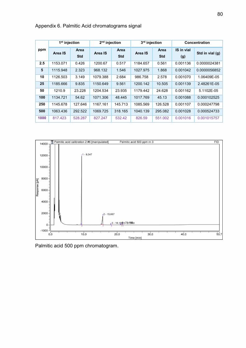
80
Appendix 6. Palmitic Acid chromatograms signal
ppm
1st injection 2nd injection 3rd injection Concentration
Area IS Area
Std Area IS
Area
Std Area IS
Area
Std
IS in vial
(g) Std in vial (g)
2.5 1153.071 0.426 1200.67 0.517 1184.657 0.561 0.001136 0.0000024381
5 1115.948 2.323 968.132 1.546 1027.975 1.868 0.001042 0.0000056852
10 1126.503 3.149 1079.388 2.684 986.758 2.578 0.001070 1.06409E-05
25 1185.666 9.835 1150.649 9.561 1200.142 10.505 0.001139 2.48261E-05
50 1210.9 23.228 1204.534 23.935 1179.442 24.628 0.001162 5.1102E-05
100 1134.721 54.62 1071.306 48.445 1017.769 45.13 0.001088 0.000102525
250 1145.678 127.646 1167.161 145.713 1085.569 126.528 0.001107 0.000247798
500 1063.436 292.522 1069.725 318.165 1040.139 295.082 0.001028 0.000524733
1000 817.423 528.287 827.247 532.42 826.59 551.002 0.001016 0.001015757
Palmitic acid 500 ppm chromatogram.
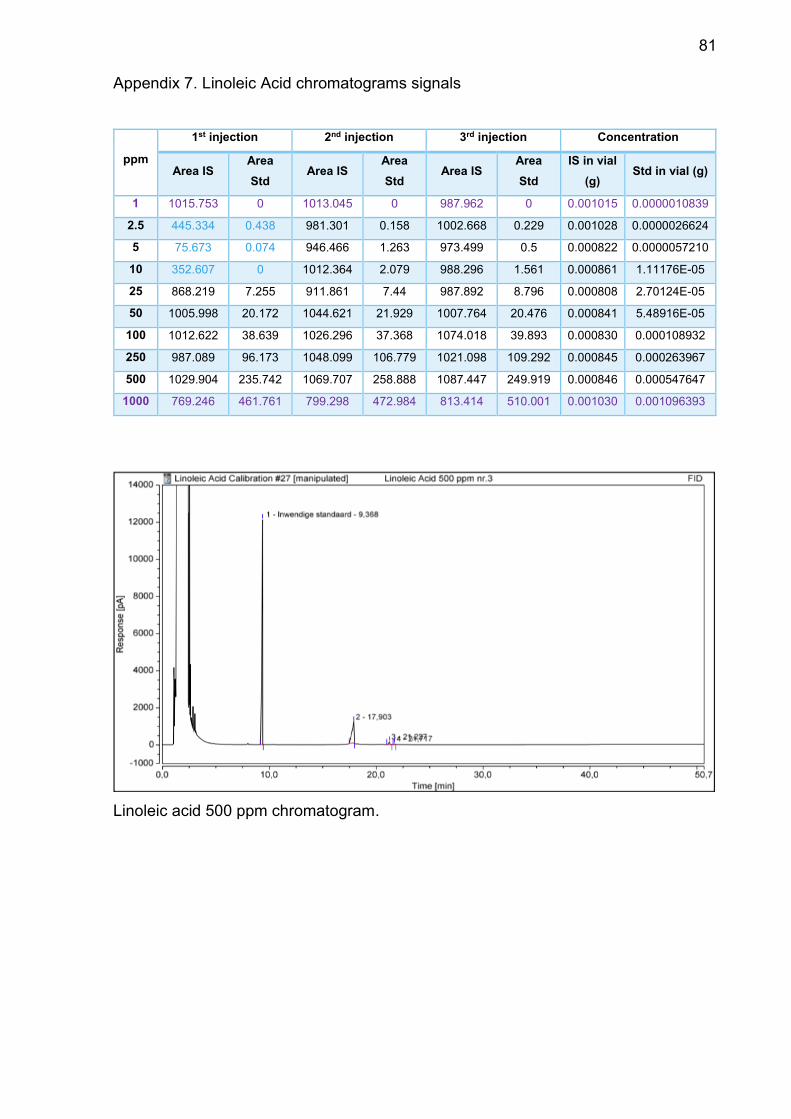
81
Appendix 7. Linoleic Acid chromatograms signals
ppm
1st injection 2nd injection 3rd injection Concentration
Area IS Area
Std Area IS
Area
Std Area IS
Area
Std
IS in vial
(g) Std in vial (g)
1 1015.753 0 1013.045 0 987.962 0 0.001015 0.0000010839
2.5 445.334 0.438 981.301 0.158 1002.668 0.229 0.001028 0.0000026624
5 75.673 0.074 946.466 1.263 973.499 0.5 0.000822 0.0000057210
10 352.607 0 1012.364 2.079 988.296 1.561 0.000861 1.11176E-05
25 868.219 7.255 911.861 7.44 987.892 8.796 0.000808 2.70124E-05
50 1005.998 20.172 1044.621 21.929 1007.764 20.476 0.000841 5.48916E-05
100 1012.622 38.639 1026.296 37.368 1074.018 39.893 0.000830 0.000108932
250 987.089 96.173 1048.099 106.779 1021.098 109.292 0.000845 0.000263967
500 1029.904 235.742 1069.707 258.888 1087.447 249.919 0.000846 0.000547647
1000 769.246 461.761 799.298 472.984 813.414 510.001 0.001030 0.001096393
Linoleic acid 500 ppm chromatogram.
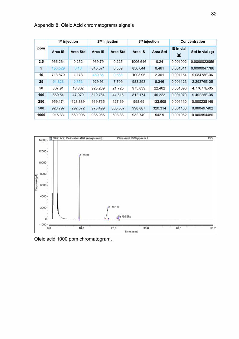
82
Appendix 8. Oleic Acid chromatograms signals
ppm
1st injection 2nd injection 3rd injection Concentration
Area IS Area Std Area IS Area Std Area IS Area Std IS in vial
(g) Std in vial (g)
2.5 966.264 0.252 969.79 0.225 1006.646 0.24 0.001002 0.0000023056
5 150.529 0.16 840.071 0.509 856.644 0.461 0.001011 0.0000047786
10 713.879 1.173 459.85 0.583 1003.96 2.301 0.001154 9.08478E-06
25 94.828 0.353 929.93 7.709 983.293 8.346 0.001123 2.29376E-05
50 867.91 18.862 923.209 21.725 975.839 22.402 0.001096 4.77677E-05
100 860.54 47.979 819.784 44.516 812.174 46.222 0.001070 9.40225E-05
250 959.174 128.889 939.735 127.69 998.69 133.608 0.001110 0.000235149
500 920.797 292.672 978.499 305.367 998.887 320.314 0.001100 0.000497402
1000 915.33 560.008 935.985 603.33 932.749 542.9 0.001062 0.000954486
Oleic acid 1000 ppm chromatogram.
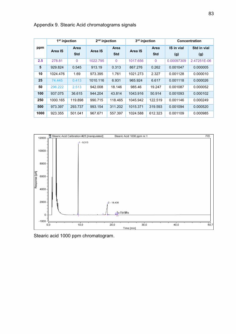
83
Appendix 9. Stearic Acid chromatograms signals
ppm
1st injection 2nd injection 3rd injection Concentration
Area IS Area
Std Area IS
Area
Std Area IS
Area
Std
IS in vial
(g)
Std in vial
(g)
2.5 278.81 0 1022.795 0 1017.656 0 0.00097309 2.47251E-06
5 929.824 0.545 913.19 0.313 867.276 0.262 0.001047 0.000005
10 1024.476 1.69 973.395 1.761 1021.273 2.327 0.001128 0.000010
25 74.445 0.413 1010.116 6.931 965.924 6.617 0.001118 0.000026
50 296.222 2.513 942.008 18.146 985.46 19.247 0.001087 0.000052
100 937.075 36.615 944.204 43.814 1043.916 50.914 0.001093 0.000102
250 1000.165 119.898 990.715 118.465 1045.942 122.519 0.001146 0.000249
500 973.397 293.737 993.154 311.202 1015.371 319.593 0.001094 0.000520
1000 923.355 501.041 967.671 557.397 1024.588 612.323 0.001109 0.000985
Stearic acid 1000 ppm chromatogram.
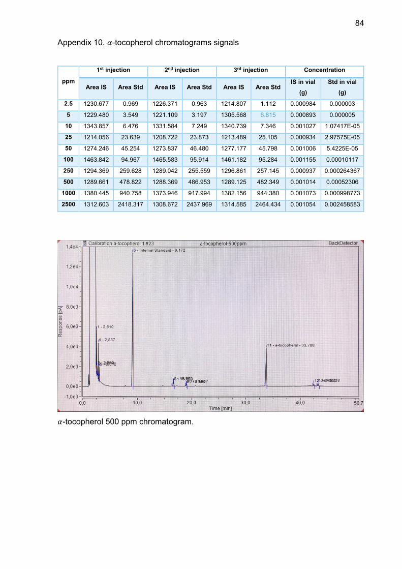
84
Appendix 10. 𝛼-tocopherol chromatograms signals
ppm
1st injection 2nd injection 3rd injection Concentration
Area IS Area Std Area IS Area Std Area IS Area Std IS in vial
(g)
Std in vial
(g)
2.5 1230.677 0.969 1226.371 0.963 1214.807 1.112 0.000984 0.000003
5 1229.480 3.549 1221.109 3.197 1305.568 6.815 0.000893 0.000005
10 1343.857 6.476 1331.584 7.249 1340.739 7.346 0.001027 1.07417E-05
25 1214.056 23.639 1208.722 23.873 1213.489 25.105 0.000934 2.97575E-05
50 1274.246 45.254 1273.837 46.480 1277.177 45.798 0.001006 5.4225E-05
100 1463.842 94.967 1465.583 95.914 1461.182 95.284 0.001155 0.00010117
250 1294.369 259.628 1289.042 255.559 1296.861 257.145 0.000937 0.000264367
500 1289.661 478.822 1288.369 486.953 1289.125 482.349 0.001014 0.00052306
1000 1380.445 940.758 1373.946 917.994 1382.156 944.380 0.001073 0.000998773
2500 1312.603 2418.317 1308.672 2437.969 1314.585 2464.434 0.001054 0.002458583
𝛼-tocopherol 500 ppm chromatogram.
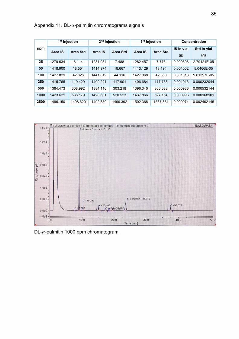
85
Appendix 11. DL-𝛼-palmitin chromatograms signals
ppm
1st injection 2nd injection 3rd injection Concentration
Area IS Area Std Area IS Area Std Area IS Area Std IS in vial
(g)
Std in vial
(g)
25 1279.634 8.114 1281.934 7.488 1282.457 7.776 0.000898 2.79121E-05
50 1418.900 18.554 1414.974 18.667 1413.129 18.194 0.001002 5.0466E-05
100 1427.829 42.828 1441.819 44.116 1427.068 42.860 0.001018 9.81397E-05
250 1415.765 119.429 1409.221 117.901 1406.684 117.788 0.001016 0.000232044
500 1384.473 308.992 1384.116 303.218 1396.340 306.638 0.000936 0.000532144
1000 1423.621 536.179 1420.631 520.523 1437.866 527.164 0.000993 0.000968901
2500 1496.150 1498.620 1492.880 1499.392 1502.368 1567.881 0.000974 0.002402145
DL-𝛼-palmitin 1000 ppm chromatogram.
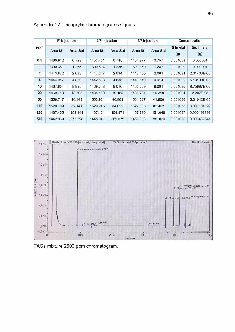
86
Appendix 12. Tricaprylin chromatograms signals
ppm
1st injection 2nd injection 3rd injection Concentration
Area IS Area Std Area IS Area Std Area IS Area Std IS in vial
(g)
Std in vial
(g)
0.5 1460.912 0.723 1453.451 0.745 1454.977 0.757 0.001063 0.000001
1 1390.381 1.265 1390.504 1.236 1393.369 1.287 0.001000 0.000001
2 1443.872 2.033 1447.247 2.034 1443.460 2.061 0.001034 2.01403E-06
5 1444.917 4.860 1442.863 4.835 1446.149 4.914 0.001030 5.13139E-06
10 1467.654 8.895 1469.748 9.016 1465.059 9.091 0.001036 9.75697E-06
20 1469.713 18.705 1484.180 19.185 1488.784 19.319 0.001034 2.207E-05
50 1556.717 40.343 1553.961 40.863 1561.027 41.808 0.001086 5.01042E-05
100 1520.709 82.141 1529.245 84.025 1527.005 82.462 0.001058 0.000104099
200 1467.455 152.141 1467.124 154.971 1457.790 151.046 0.001037 0.000198992
500 1442.969 375.398 1448.041 389.075 1453.313 381.020 0.001020 0.000489547
TAGs mixture 2500 ppm chromatogram.
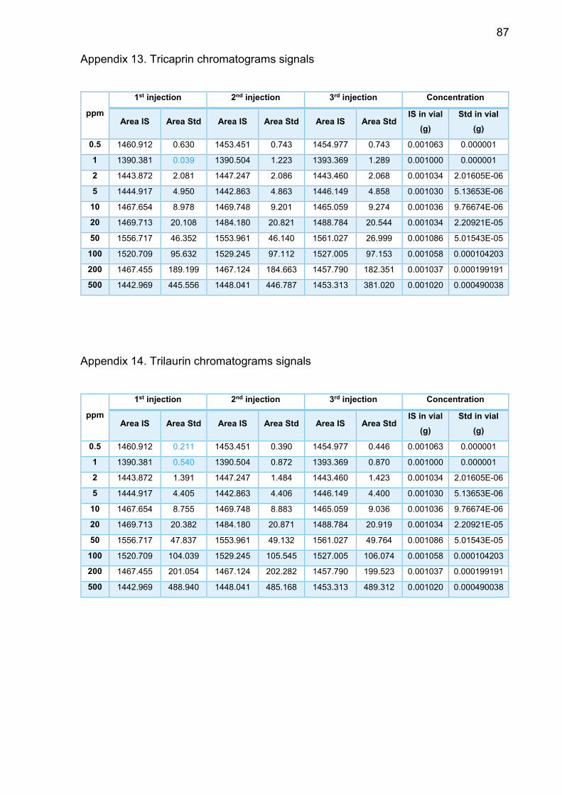
87
Appendix 13. Tricaprin chromatograms signals
ppm
1st injection 2nd injection 3rd injection Concentration
Area IS Area Std Area IS Area Std Area IS Area Std IS in vial
(g)
Std in vial
(g)
0.5 1460.912 0.630 1453.451 0.743 1454.977 0.743 0.001063 0.000001
1 1390.381 0.039 1390.504 1.223 1393.369 1.289 0.001000 0.000001
2 1443.872 2.081 1447.247 2.086 1443.460 2.068 0.001034 2.01605E-06
5 1444.917 4.950 1442.863 4.863 1446.149 4.858 0.001030 5.13653E-06
10 1467.654 8.978 1469.748 9.201 1465.059 9.274 0.001036 9.76674E-06
20 1469.713 20.108 1484.180 20.821 1488.784 20.544 0.001034 2.20921E-05
50 1556.717 46.352 1553.961 46.140 1561.027 26.999 0.001086 5.01543E-05
100 1520.709 95.632 1529.245 97.112 1527.005 97.153 0.001058 0.000104203
200 1467.455 189.199 1467.124 184.663 1457.790 182.351 0.001037 0.000199191
500 1442.969 445.556 1448.041 446.787 1453.313 381.020 0.001020 0.000490038
Appendix 14. Trilaurin chromatograms signals
ppm
1st injection 2nd injection 3rd injection Concentration
Area IS Area Std Area IS Area Std Area IS Area Std IS in vial
(g)
Std in vial
(g)
0.5 1460.912 0.211 1453.451 0.390 1454.977 0.446 0.001063 0.000001
1 1390.381 0.540 1390.504 0.872 1393.369 0.870 0.001000 0.000001
2 1443.872 1.391 1447.247 1.484 1443.460 1.423 0.001034 2.01605E-06
5 1444.917 4.405 1442.863 4.406 1446.149 4.400 0.001030 5.13653E-06
10 1467.654 8.755 1469.748 8.883 1465.059 9.036 0.001036 9.76674E-06
20 1469.713 20.382 1484.180 20.871 1488.784 20.919 0.001034 2.20921E-05
50 1556.717 47.837 1553.961 49.132 1561.027 49.764 0.001086 5.01543E-05
100 1520.709 104.039 1529.245 105.545 1527.005 106.074 0.001058 0.000104203
200 1467.455 201.054 1467.124 202.282 1457.790 199.523 0.001037 0.000199191
500 1442.969 488.940 1448.041 485.168 1453.313 489.312 0.001020 0.000490038
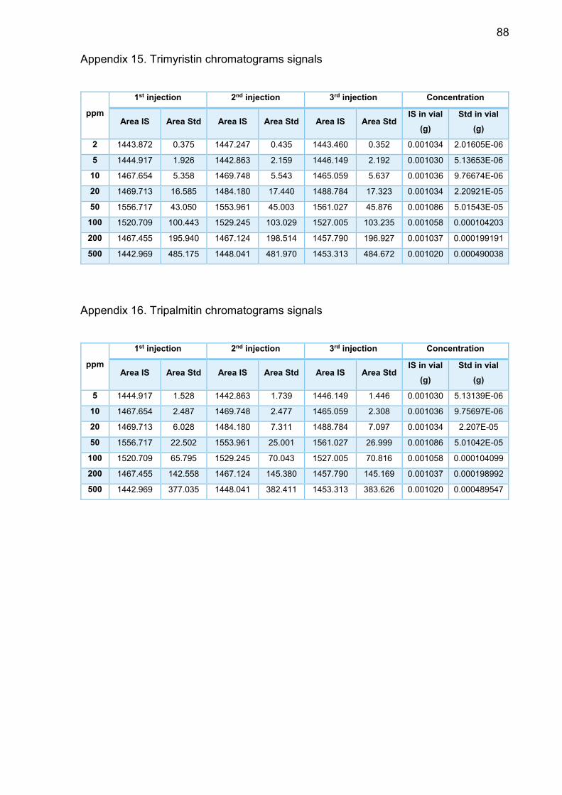
88
Appendix 15. Trimyristin chromatograms signals
ppm
1st injection 2nd injection 3rd injection Concentration
Area IS Area Std Area IS Area Std Area IS Area Std IS in vial
(g)
Std in vial
(g)
2 1443.872 0.375 1447.247 0.435 1443.460 0.352 0.001034 2.01605E-06
5 1444.917 1.926 1442.863 2.159 1446.149 2.192 0.001030 5.13653E-06
10 1467.654 5.358 1469.748 5.543 1465.059 5.637 0.001036 9.76674E-06
20 1469.713 16.585 1484.180 17.440 1488.784 17.323 0.001034 2.20921E-05
50 1556.717 43.050 1553.961 45.003 1561.027 45.876 0.001086 5.01543E-05
100 1520.709 100.443 1529.245 103.029 1527.005 103.235 0.001058 0.000104203
200 1467.455 195.940 1467.124 198.514 1457.790 196.927 0.001037 0.000199191
500 1442.969 485.175 1448.041 481.970 1453.313 484.672 0.001020 0.000490038
Appendix 16. Tripalmitin chromatograms signals
ppm
1st injection 2nd injection 3rd injection Concentration
Area IS Area Std Area IS Area Std Area IS Area Std IS in vial
(g)
Std in vial
(g)
5 1444.917 1.528 1442.863 1.739 1446.149 1.446 0.001030 5.13139E-06
10 1467.654 2.487 1469.748 2.477 1465.059 2.308 0.001036 9.75697E-06
20 1469.713 6.028 1484.180 7.311 1488.784 7.097 0.001034 2.207E-05
50 1556.717 22.502 1553.961 25.001 1561.027 26.999 0.001086 5.01042E-05
100 1520.709 65.795 1529.245 70.043 1527.005 70.816 0.001058 0.000104099
200 1467.455 142.558 1467.124 145.380 1457.790 145.169 0.001037 0.000198992
500 1442.969 377.035 1448.041 382.411 1453.313 383.626 0.001020 0.000489547