detection of targets in noise and pulse compression techniques
TRANSCRIPT

Radar Course_1.pptODonnell 6-18-02
MIT Lincoln Laboratory
Introduction to Radar Systems
Detection of Targets in Noise and
Pulse Compression Techniques

MIT Lincoln LaboratoryRadar Course_2.pptODonnell 10-26-01
Disclaimer of Endorsement and Liability
• The video courseware and accompanying viewgraphs presented on this server were prepared as an account of work sponsored by an agency of the United States Government. Neither the United States Government nor any agency thereof, nor any of their employees, nor the Massachusetts Institute of Technology and its Lincoln Laboratory, nor any of their contractors, subcontractors, or their employees, makes any warranty, express or implied, or assumes any legal liability or responsibility for the accuracy, completeness, or usefulness of any information, apparatus, products, or process disclosed, or represents that its use would not infringe privately owned rights. Reference herein to any specific commercial product, process, or service by trade name, trademark, manufacturer, or otherwise does not necessarily constitute or imply its endorsement, recommendation, or favoring by the United States Government, any agency thereof, or any of their contractors or subcontractors or the Massachusetts Institute of Technology and its Lincoln Laboratory.
• The views and opinions expressed herein do not necessarily state or reflect those of the United States Government or any agency thereof or any of their contractors or subcontractors

MIT Lincoln LaboratoryRadar Course_3.pptODonnell 10-26-01
Detection and Pulse Compression
Transmitter
PulseCompression
Recording
Receiver
Tracking &ParameterEstimation
Console /Display
Antenna
PropagationMedium
TargetCross
Section DopplerProcessingA / D
WaveformGenerator
Detection
Signal Processor
Main Computer

MIT Lincoln LaboratoryRadar Course_4.pptODonnell 10-26-01
Outline
• Detection of Target Echoes in Noise– Basic Concepts
– Integration of Pulses
– Fluctuating Targets Issues
– Adaptive Thresholding Techniques
• Pulse Compression

MIT Lincoln LaboratoryRadar Course_5.pptODonnell 10-26-01
Target Detection in the Presence of Noise
0 10 20 30 40 50 60 70 80 90 100-20
-15
-10
-5
0
5
10
15
Range Gate
Rel
ativ
e Po
wer
(dB
)Noise TargetsThreshold
DetectableMarginal
Undetectable
321-00395DPC 9/8/2008
• The radar return is sampled at regular intervals with A/D (Analog to Digital) converters
• The sampled returns may include the target of interest and noise
• A threshold is used to reject noise

MIT Lincoln LaboratoryRadar Course_6.pptODonnell 10-26-01
The Detection Problem
0 1 2 3 4 5 6 7 80
0.1
0.2
0.3
0.4
0.5
0.6
Prob
abili
ty D
ensi
ty Noise DetectionThreshold
Probabilityof FalseAlarms
Noise Voltage
• The area under the noise probability curve, from the detection threshold to infinity (way, way out to the right) is the probability of false alarm.
• The entire area under the noise density curve is 1.

MIT Lincoln LaboratoryRadar Course_7.pptODonnell 10-26-01
The Detection Problem
Probabilityof FalseAlarms
Voltage
0 1 2 3 4 5 6 7 80
0.1
0.2
0.3
0.4
0.5
0.6
Prob
abili
ty D
ensi
ty Noise
SNR = 15 dB
Signal + Noise
DetectionThreshold PD = Detection Probability

MIT Lincoln LaboratoryRadar Course_8.pptODonnell 10-26-01
0 2 4 6 8 10 12 14 160
0.1
0.2
0.3
0.4
0.5
0.6
Prob
abili
ty D
ensi
ty
Noise
Signal-to-Noise Ratio = 15 dB
Signal + Noise
DetectionThreshold
PD(Detection
Probability)
0 2 4 6 8 10 12 14 160
0.1
0.2
0.3
0.4
0.5
0.6 Noise
Signal + Noise
VoltageVoltage
Higher PD(Detection
Probability)
Probabilityof FalseAlarm
Detection Examples with Different SNR
DetectionThreshold
Signal-to-Noise Ratio = 20 dB
For a fixed threshold, a higher SNR (or S/N) will result in a higher of probability of detecting the target

MIT Lincoln LaboratoryRadar Course_9.pptODonnell 10-26-01
Probability of Detection vs. SNR
Figure by MIT OCW.
Numbers to Remember

MIT Lincoln LaboratoryRadar Course_10.pptODonnell 10-26-01
Outline
• Detection of Target Echoes in Noise– Basic Concepts
– Integration of Pulses
– Fluctuating Targets Issues
– Adaptive Thresholding Techniques
• Pulse Compression

MIT Lincoln LaboratoryRadar Course_11.pptODonnell 10-26-01
Integration of Radar Pulses
• Improve ability of radar to detect targets by combining the returns from multiple pulses
• Coherent Integration– No information lost (amplitude or phase)
• Non-coherent integration techniques– Some information lost (phase)– Non-coherent (video) Integration– Binary Integration – Cumulative detection– For most cases, coherent integration is more efficient than non-
coherent integration

MIT Lincoln LaboratoryRadar Course_12.pptODonnell 10-26-01
Coherent Integration
• Real and Imaginary (In-phase and Quadrature) parts of the complex radar return are added, and the magnitude of the voltage is calculated
– V=(I2 + Q2 )1/2
• This quantity is then thresholded• The coherent integration gain is equal to the number of pulses
coherently integrated– 2 pulses 3 dB– 10 pulses 10 dB– 20 pulses 13 dB
• For this gain to be realized, the noise samples, from pulse to pulse must be independent
– The background noise is white Gaussian noise

MIT Lincoln LaboratoryRadar Course_13.pptODonnell 10-26-01
Noncoherent Integration Steady Target
0
1
23
4
5
0 20 40 60 80 1000
1
23
4
5
Range Gates
Nor
mal
ized
Pow
erSingle Pulse
8 Pulses Noncoherently Averaged
SNR Unchanged
Noise Variance Reduced after Integration (Allows Lower Threshold)

MIT Lincoln LaboratoryRadar Course_14.pptODonnell 10-26-01
Different Types of Non-Coherent Integration
• Non Coherent Integration – General (aka video integration) – Generate magnitude for each of N pulses
– Add magnitudes and then threshold
• Binary Integration– Generate magnitude for each of N pulses and then threshold
– Require at least M detections in N scans
• Cumulative Detection– Generate magnitude for each of N pulses and then threshold
– Require at least 1 detection in N scans

MIT Lincoln LaboratoryRadar Course_15.pptODonnell 10-26-01
Outline
• Detection of Target Echoes in Noise– Basic Concepts
– Integration of Pulses
– Fluctuating Targets Issues
– Adaptive Thresholding Techniques
• Pulse Compression

MIT Lincoln LaboratoryRadar Course_16.pptODonnell 10-26-01
Target Fluctuations Swerling Models
Nature ofScatterers
Fluctuation Interval
scan-to-scan(multiple pulses/scan)
pulse-to-pulse
similar amplitudes
one amplitude muchlarger than others
Swerling I Swerling II
Swerling III Swerling IV
( ) av
av
1 σσ−
σ=σ ep
( ) av2
2av
4 σσ−
σσ
=σ ep
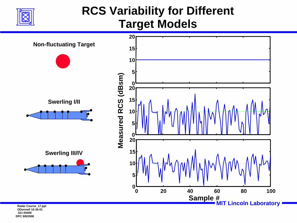
MIT Lincoln LaboratoryRadar Course_17.pptODonnell 10-26-01
RCS Variability for Different Target Models
0
5
10
15
20
0
5
10
15
20
Mea
sure
d R
CS
(dB
sm)
0 20 40 60 80 1000
5
10
15
20
Sample #
Non-fluctuating Target
Swerling I/II
Swerling III/IV
321-00400DPC 9/8/2008

MIT Lincoln LaboratoryRadar Course_18.pptODonnell 10-26-01
Detection Statistics for Fluctuating Targets Single Pulse Detection
Fluctuating Targets Require More SNR than Non-fluctuatingTargets to Maintain a High Probability of Detection
Figure by MIT OCW.

MIT Lincoln LaboratoryRadar Course_19.pptODonnell 10-26-01
Outline
• Detection of Target Echoes in Noise– Basic Concepts
– Integration of Pulses
– Fluctuating Targets Issues
– Adaptive Thresholding Techniques
• Pulse Compression

MIT Lincoln LaboratoryRadar Course_20.pptODonnell 10-26-01
Constant False Alarm Rate (CFAR) Thresholding
• Problem: Must know (or estimate) noise floor to set threshold
• Solution: Estimate noise floor using noise-only samples
– Adaptive thresholding
• CFAR thresholding:
0 20 40 60 80 100Time (µs)
0
10
20
30
40
Pow
er (d
B)
Signal
Noise floor
Absolutethreshold False alarm
test cellnoise floor estimate > threshold

MIT Lincoln LaboratoryRadar Course_21.pptODonnell 10-26-01
The Mean Level CFAR
• Use mean value of surrounding range cells to determine threshold for cell under test
• Nearby targets can raise threshold and suppress detection
Cell Under Test
“Guard” Cells
Data Cells for Mean Level Computation
Window Slides Through Data

MIT Lincoln LaboratoryRadar Course_22.pptODonnell 10-26-01
Effect of Rain on CFAR Thresholding
Cell Under Test
“Guard” Cells
Data Cells for Mean Level Computation
Window Slides Through Data
2.2 dB9 dB
4.52.6 Slant Range, nmi
Rad
ar B
acks
catte
r (Li
near
Uni
ts)
Rain Cloud
C Band5500 MHz
Receiver NoiseReceiver Noise
Range Cells

MIT Lincoln LaboratoryRadar Course_23.pptODonnell 10-26-01
Effect of Rain on CFAR Thresholding
2.2 dB9 dB
4.52.6 Slant Range, nmi
Am
plitu
de (L
inea
r Uni
ts)
Rain Cloud
C Band5500 MHz
Range Cells
Cell Under Test
“Guard” Cells
Data Cells for Mean Level Computation
Window Slides Through Data
Receiver NoiseReceiver Noise
Sharp Clutter or Interference Boundaries Can Lead to Excessive False Alarms

MIT Lincoln LaboratoryRadar Course_24.pptODonnell 10-26-01
Greatest-of Mean Level CFAR
• Find mean value of N/2 cells before and after test cell separately
• Use larger noise estimate to determine threshold
• Helps reduce false alarms near sharp clutter or interference boundaries
• Nearby targets still raise threshold and suppress detection
Cell Under Test
“Guard” CellsData Cells for Mean Level 1
Window Slides Through Data
Data Cells for Mean Level 2
Use Larger Value

MIT Lincoln LaboratoryRadar Course_25.pptODonnell 10-26-01
Outline
• Detection of Target Echoes in Noise
• Pulse Compression– Introduction
– Phase Coded Waveforms
– Linear Frequency Modulation Waveforms

MIT Lincoln LaboratoryRadar Course_26.pptODonnell 10-26-01
Pulsed CW Radar Fundamentals Range Resolution
• Range Resolution ( )– Proportional to pulse width (T)
– Inversely proportional to bandwidth (B = 1/T)1 MHz Bandwidth => 150 m of range resolution B
cr
cr
2
2
=Δ
=Δ T
T
1 2 3 4
1
2
3
0
Am
plitu
de
0
10
20
-20
Pow
er (d
B)
0 2 3 4 51
Frequency (MHz)Time (μsec)
T1
BandwidthPulsewidth
1 μsec pulse Frequency spectrum of pulse
rΔ

MIT Lincoln LaboratoryRadar Course_27.pptODonnell 10-26-01
Pulse Width, Bandwidth and Resolution for a Square Pulse
Cannot Resolve Features Along the Target
Can Resolve Features Along the Target
Pulse Length is Larger than Target Length
Pulse Length is Smaller than Target Length
Resolution:
Shorter Pulses have Higher Bandwidth and Better Resolution
Bcr
cr
2
2
=Δ
=Δ T
-40
-20
0
Example :High BandwidthΔr = .1 x Δ
rBW = 10 x BWLow Bandwidth
Relative Range (m)
Rel
ativ
eR
CS
(dB
)

MIT Lincoln LaboratoryRadar Course_28.pptODonnell 10-26-01
Motivation for Pulse Compression
• Hard to get “good” average power and resolution at the same time using a pulsed CW system
– Higher average power is proportional to pulse width
– Better resolution is inversely proportional to pulse width
• A long pulse can have the same bandwidth (resolution) as a short pulse if the long pulse is modulated in frequency or phase
• These pulse compression techniques allow a radar to simultaneously achieve the energy of a long pulse and the resolution of a short pulse

MIT Lincoln LaboratoryRadar Course_29.pptODonnell 10-26-01
Matched Filter Concept
MatchedFilter
2EN0
E = Pulse Energy (Power × Time)
Pulse Spectrum
Am
plitu
de Phase
Frequency
Matched FilterA
mpl
itude Phase
Frequency
Noise Spectrum
Am
plitu
de
Frequency
N0
Fourier Transform
• Matched Filter maximizes the peak-signal to mean noise ratio– For rectangular pulse, matched filter is a simple pass band filter

MIT Lincoln LaboratoryRadar Course_30.pptODonnell 10-26-01
Frequency and Phase Modulation of Pulses
• Resolution of a short pulse can be achieved by modulating a long pulse, increasing the time-bandwidth product
• Signal must be processed on return to “pulse compress”
Binary PhaseCoded Waveform
Linear FrequencyModulated Waveform
Bandwidth = 1/TCHIP
Pulse Width, T
Frequency F1 Frequency F2Bandwidth = ΔF = F2-F1
Square PulsePulse Width, TPulse Width, T
TCHIP
Bandwidth = 1/T
Time × Bandwidth = 1 Time × Bandwidth = T/TCHIP Time × Bandwidth = TΔF

MIT Lincoln LaboratoryRadar Course_31.pptODonnell 10-26-01
Binary Phase Coded Waveforms
• Changes in phase can be used to increase the signal bandwidth of a long pulse
• A pulse of duration T is divided into N sub-pulses of duration TCHIP
• The phase of each sub-pulse is changed or not changed, according to a binary phase code
• Phase changes 0 or π radians (+ or -) • Pulse compression filter output will
be a compressed pulse of width TCHIP and a peak N times that of the uncompressed pulse
Binary PhaseCoded Waveform
Bandwidth = 1/ TCHIP
Pulse Width, T
TCHIP
Pulse Compression Ratio = T/ TCHIP

MIT Lincoln LaboratoryRadar Course_32.pptODonnell 10-26-01
• Matched filter is implemented by “convolving” the reflected echo with the “time reversed” transmit pulse
• Convolution process: – Move digitized pulses by each other, in steps
– When data overlaps, multiply samples and sum them up
Reflected echo Time reversed pulse
Implementation of Matched Filter
1
3
1
2
0No overlap – Output 0
Out
put o
f M
atch
ed F
ilter
Time

MIT Lincoln LaboratoryRadar Course_33.pptODonnell 10-26-01
• Matched filter is implemented by “convolving” the reflected echo with the “time reversed” transmit pulse
• Convolution process: – Move digitized pulses by each other, in steps
– When data overlaps, multiply samples and sum them up
Reflected echo Time reversed pulse
Implementation of Matched Filter
1
3
1
2
0No overlap – Output 0
Out
put o
f M
atch
ed F
ilter
Time

MIT Lincoln LaboratoryRadar Course_34.pptODonnell 10-26-01
• Matched filter is implemented by “convolving” the reflected echo with the “time reversed” transmit pulse
• Convolution process: – Move digitized pulses by each other, in steps
– When data overlaps, multiply samples and sum them up
Reflected echo Time reversed pulse
Implementation of Matched Filter
1
3
1
2
0One sample overlaps 1x1 =1
Out
put o
f M
atch
ed F
ilter
Time

MIT Lincoln LaboratoryRadar Course_35.pptODonnell 10-26-01
• Matched filter is implemented by “convolving” the reflected echo with the “time reversed” transmit pulse
• Convolution process: – Move digitized pulses by each other, in steps
– When data overlaps, multiply samples and sum them up
Reflected echo Time reversed pulse
Implementation of Matched Filter
1
3
1
2
0Two samples overlap (1x1) + (1x1) = 2
Out
put o
f M
atch
ed F
ilter
Time

MIT Lincoln LaboratoryRadar Course_36.pptODonnell 10-26-01
• Matched filter is implemented by “convolving” the reflected echo with the “time reversed” transmit pulse
• Convolution process: – Move digitized pulses by each other, in steps
– When data overlaps, multiply samples and sum them up
Reflected echo Time reversed pulse
Implementation of Matched Filter
1
3
1
2
0Three samples overlap (1x1) + (1x1) + (1x1) = 3
Out
put o
f M
atch
ed F
ilter
Time

MIT Lincoln LaboratoryRadar Course_37.pptODonnell 10-26-01
• Matched filter is implemented by “convolving” the reflected echo with the “time reversed” transmit pulse
• Convolution process: – Move digitized pulses by each other, in steps
– When data overlaps, multiply samples and sum them up
Reflected echo Time reversed pulse
Implementation of Matched Filter
1
3
1
2
0Two samples overlap (1x1) + (1x1) = 2
Out
put o
f M
atch
ed F
ilter
Time

MIT Lincoln LaboratoryRadar Course_38.pptODonnell 10-26-01
• Matched filter is implemented by “convolving” the reflected echo with the “time reversed” transmit pulse
• Convolution process: – Move digitized pulses by each other, in steps
– When data overlaps, multiply samples and sum them up
Reflected echo Time reversed pulse
Implementation of Matched Filter
1
Time
3
1
2
0
Out
put o
f M
atch
ed F
ilter
One sample overlaps 1x1 =1

MIT Lincoln LaboratoryRadar Course_39.pptODonnell 10-26-01
• Matched filter is implemented by “convolving” the reflected echo with the “time reversed” transmit pulse
• Convolution process: – Move digitized pulses by each other, in steps
– When data overlaps, multiply samples and sum them up
Reflected echo Time reversed pulse
Implementation of Matched Filter
1
Time
3
1
2
0
Out
put o
f M
atch
ed F
ilter
Use of Matched Filter Maximizes S/N

MIT Lincoln LaboratoryRadar Course_40.pptODonnell 10-26-01
Pulse Compression Binary Phase Modulation Example
Figure by MIT OCW.

MIT Lincoln LaboratoryRadar Course_41.pptODonnell 10-26-01
Linear FM Pulse Compression
Because range is measured by a shift in Doppler frequency, there is a coupling of the range and Doppler velocity measurement
Figure by MIT OCW.

MIT Lincoln LaboratoryRadar Course_42.pptODonnell 10-26-01
Summary
• Detection of Targets in Noise– Both target properties and radar design features affect the ability to
detect signals in noise– Coherent and non-coherent integration pulse integration can improve
target detection– Adaptive thresholding (CFAR) techniques are needed in realistic
environments
• Pulse compression offers a means to simultaneous have high average power and good resolution
– A long pulse can have the same bandwidth (resolution) as a short pulse, if it is modulated in frequency or phase
– Phase-encoded pulse compression divides long pulses into binary encoded sub-pulses
– With frequency-encoded pulse compression, the radar frequency is increased linearly as the pulse is transmitted

MIT Lincoln LaboratoryRadar Course_43.pptODonnell 10-26-01
References
• Skolnik, M., Introduction to Radar Systems, New York, McGraw-Hill, 3rd Edition, 2001
• Toomay, J. C., Radar Principles for the Non-Specialist, New York, Van Nostrand Reinhold, 1989