5 pulse compression waveform
TRANSCRIPT

Pulse Compression Waveform
SOLO HERMELIN
Updated: 27.10.08http://www.solohermelin.com

Table of Content
SOLO Pulse Compression Waveform
Resolution
Pulse Range Resolution
Pulse Compression Waveform Introduction
Waveform Hierarchy
Linear FM Modulated Pulse (Chirp)
Barker Codes
Combined Barker Codes
Poly-Phase Codes
Phase Coded Waveforms
Matched Filter Response to Phase Coding
Bi-Phase Codes

Table of Content (continue – 1)
SOLO Pulse Compression Waveform
Poly-Phase Codes
Frank Codes
P1, P2, P3, P4 Poly-Phase Codes
Pseudo-Random Codes
Frequency Codes
Costas Codes
Complementary Pulse Codes
Summary of Pulse Compression Codes
References

Range & Doppler Measurements in RADAR SystemsSOLO
Resolution
Resolution is the spacing (in range, Doppler, angle, etc.) we must have in order todistinguish between two different targets.
first targetresponse
second targetresponse
compositetarget
response
greather then 3 db
DistinguishableTargets
first targetresponse
second targetresponse
compositetarget
response
UndistinguishableTargets
less then 3 db
The two targets are distinguishable ifthe composite (sum) of the received signal has a deep (between the twopicks) of at least 3 db.
Return to Table of Content

SOLOUnmodulated Pulse Range Resolution
Resolution is the spacing (in range, Doppler, angle, etc.) we must have in order todistinguish between two different targets.
Range Resolution
RADAR
τ
c
R
RR ∆+
Target # 1Target # 2
Assume two targets spaced by a range Δ R and a unmodulated radar pulse of τ seconds.
The echoes start to be receivedat the radar antenna at times: 2 R/c – first target 2 (R+Δ R)/c – second target
The echo of the first target endsat 2 R/c + τ
τ τ
time from pulsetransmission
c
R2 ( )c
RR ∆+2τ+
c
R2
ReceivedSignals
Target # 1 Target # 2
The two targets echoes can beresolved if:
c
RR
c
R ∆+=+ 22 τ2
τcR =∆ Pulse Range Resolution
( ) ( ) ≤≤+
=elsewhere
ttAts
0
0cos: 0 τϕω

Unmodulated Pulse
SOLO
Energy ( ) ( ) ( )∫∫∫+∞
∞−
+∞
∞−
+∞
∞−
=== ωωπ
dSdttsdttsEs222
2
1:
( ) ( ) ≤≤+
=elsewhere
ttAts
0
0cos: 0 τϕω
( ) ( )
( )[ ] ( ) ( )
−++=++=
+==
∫
∫∫+∞
∞−
τϕϕτωτϕω
ϕω
τ
τ
0002
0
00
2
0
2
002
2cos22cos1
222cos1
2
cos
Adtt
A
dttAdttsEs
Unmodulated Pulse

RADAR SignalsSOLO
( ) ( ) ≤≤+
=elsewhere
ttAts
0
0cos: 0 τϕω
Energy( ) ( )
2
2cos22cos1
2
2000
2 ττ
ϕϕτωτ AE
AE ss =⇒
−++=
2
τcR =∆ Pulse Range Resolution
Decreasing Pulse Width Increasing
Decreasing SNR, Radar Performance Increasing
Increasing Range Resolution Capability Decreasing
For the Unmodulated Pulse, there exists a coupling between Range Resolution andWaveform Energy. Return to Table of Content

Pulse Compression WaveformsSOLO
Pulse Compression Waveforms permit a decoupling between Range Resolution and Waveform Energy.
- An increased waveform bandwidth (BW) relative to that achievable with an unmodulated pulse of an equal duration
τ1>>BW
22
τcBW
cR <<=∆
- Waveform duration in excess of that achievable with unmodulated pulse of equivalent waveform bandwidth
BW
1>>τ
PCWF exhibit the following equivalent properties:
This is accomplished by modulating (or coding) the transmit waveform and compressing the resulting received waveform.
Pulse Compression Waveform Introduction
Return to Table of Content

SOLO Waveform Hierarchy
Radar Waveforms
CW Radars Pulsed Radars
FrequencyModulated CW
PhaseModulated CW
bi – phase & poly-phase
Linear FMCWSawtooth, or
Triangle
Nonlinear FMCWSinusoidal,
Multiple Frequency,Noise, Pseudorandom
Intra-pulse Modulation
Pulse-to-pulse Modulation,
Frequency AgilityStepped Frequency
FrequencyModulate Linear FM
Nonlinear FM
PhaseModulatedbi – phase poly-phase
Unmodulated CW
Multiple FrequencyFrequency
Shift Keying
Fixed Frequency

SOLO Waveform Hierarchy
• Pulse Compression Techniques• Wave Coding
• Frequency Modulation (FM)
- Linear
• Phase Modulation (PM)]
- Non-linear
- Pseudo-Random Noise (PRN)
- Bi-phase (0º/180º)
- Quad-phase (0º/90º/180º/270º)
• Implementation
• Hardware
- Surface Acoustic Wave (SAW) expander/compressor
• Digital Control- Direct Digital Synthesizer (DDS)
- Software compression “filter”Return to Table of Content

SOLO
• Pulse Compression Techniques

SOLO
• Pulse Compression Techniques

SOLO Waveform Hierarchy• Pulse Compression Techniques

SOLO Coherent Pulse Doppler Radar
Return to Table of Content

SOLO
Linear FM Modulated Pulse (Chirp)
( ) ( )2/cos 203 ttAtf ωω ∆+=
t
A
2/τ−2/τ ( )
222cos
2
0
ττµω ≤≤−
+= tt
tAtsi
Pulse Compression Waveforms
Linear Frequency Modulation is a technique used to increase the waveform bandwidthBW while maintaining pulse duration τ, such that
BW
1>>τ 1>>⋅BWτ
222 0
2
0
ττµωµωω ≤≤−+=
+= tt
tt
td
d

Matched Filters for RADAR Signals
( ) ( )( ) ( )
≤≤−== −∗
Ttttsth
eSH
i
tji
00
0ωωω
SOLO
The Matched Filter (Summary(
si (t) - Signal waveform
Si (ω) - Signal spectral density
h (t) - Filter impulse response
H (ω) - Filter transfer function
t0 - Time filter output is sampled
n (t) - noise
N (ω) - Noise spectral density
Matched Filter is a linear time-invariant filter hopt (t) that maximizesthe output signal-to-noise ratio at a predefined time t0, for a given signal si (t(.
The Matched Filter output is:
( ) ( ) ( ) ( ) ( )
( ) ( ) ( ) ( ) ( ) 00
00
tjiii
iii
eSSHSS
dttssdthsts
ωωωωωω
ξξξξξξ
−∗
+∞
∞−
+∞
∞−
⋅=⋅=
+−=−= ∫∫

SOLO
Linear FM Modulated Pulse (continue – 1)
Pulse Compression Waveforms
Concept of Group Delay
BW
1>>τ
τ
BW
1
( )222
cos2
0
ττµω ≤≤−
+= tt
tAtsi
( ) ( )222
cos2
0
00 ττµω ≤≤−
−=−=
=
tt
tAtsth i
t
MF
Matched Filter
( )tsi ( )tso
( ) ( )tsth i
t
MF −==00 ( ) ( ) ( ) ( ) ( )
( ) ( ) ( ) ( ) ( )ωωωωω
ξξξξξξ
∗=
+∞
∞−
=+∞
∞−
⋅=⋅=
−=−= ∫∫
ii
t
i
ii
t
i
SSHSS
dtssdthsts
0
0
0
0
0
0

SOLO
Linear FM Modulated Pulse (continue – 2)
Pulse Compression Waveforms
Concept of Group Delay (continue -1)
BW
1>>τ
τ
BW
1
( )222
cos2
0
ττµω ≤≤−
+= tt
tAtsi
Matched Filter
( )tsi ( )tso
( ) ( )tsth i
t
MF −==00 ( ) ( ) ( ) ( ) ( )
( ) ( ) ( ) ( ) ( )ωωωωω
ξξξξξξ
∗=
+∞
∞−
=+∞
∞−
⋅=⋅=
−=−= ∫∫
ii
t
i
ii
t
i
SSHSS
dtssdthsts
0
0
0
0
0
0
( ) ( ) ( ) ( )
>≤≤+−
<+≤≤−
−+−
+=−
022
022
2cos
2cos
2
0
2
02
tt
ttt
tAtss ii τξτ
τξτξµξωξµξωξξ
( ) ( ) ( ) ( ) ( )∫∫
+
+−
>∞+
∞−
>=
−+−
+=−=
2/
2/
2
0
2
02
000
0 2cos
2cos
0 τ
τ
ξξµξωξµξωξξξt
t
ii
tt
dt
tAdtssts
( ) ( )222
cos2
0
00 ττµω ≤≤−
−=−=
=
tt
tAtsth i
t
MF
Ignoring terms of 2 ω0
( ) ( ) ( )
( ) ( )t
tttA
t
tttA
t
tttAdttt
Ats
tt
tt
µµτµω
µµτµω
µµξµωξµξµω
τ
τ
τ
τ
2/2/sin
2
2/2/sin
2
2/sin
22/cos
22
022
02
2/
2/
20
22/
2/
20
200
0
0
+−−−+=
−+=−+≅+
+−
+
+−
>=
∫
( ) ( ) βαβαβα coscos2coscos =−++( )[ ] ( )∫∫+
+−
+
+−
−+++−+−=2/
2/
20
22/
2/
220
2
2/cos2
2/2/2cos2
τ
τ
τ
τ
ξµξµωξµξµξµξωtt
dttA
dttA

SOLO
Linear FM Modulated Pulse (continue – 3)
Pulse Compression Waveforms
Concept of Group Delay (continue -2)
BW
1>>τ
τ
BW
1
( )222
cos2
0
ττµω ≤≤−
+= tt
tAtsi
Matched Filter
( )tsi ( )tso
( ) ( )tsth i
t
MF −==00 ( ) ( ) ( ) ( ) ( )
( ) ( ) ( ) ( ) ( )ωωωωω
ξξξξξξ
∗=
+∞
∞−
=+∞
∞−
⋅=⋅=
−=−= ∫∫
ii
t
i
ii
t
i
SSHSS
dtssdthsts
0
0
0
0
0
0
( ) ( )222
cos2
0
00 ττµω ≤≤−
−=−=
=
tt
tAtsth i
t
MF
Ignoring terms of 2 ω0 ( ) ( ) ( )t
tttA
t
tttAts
tt
µµτµω
µµτµω 2/2/sin
2
2/2/sin
2
20
220
200
0
0
+−−−+≅>=
( ) ( )ttt
tt
tAts
tt
0
200
0 cos1
2
12
sin
12
0
ω
ττµ
ττµ
ττ
−
−
−≅
>= ( ) ( ) βαβαβα sincos2sinsin =−−+
−==
ττµβωα tt
t 12
,0
If we re-due for t < 0 and combine, we obtain
( ) ( )ttt
tt
tAts
t
0
20
0 cos
12
12
sin
12
0
ω
ττµ
ττµ
ττ
−
−
−≅
=

SOLO
( ) ( )2/cos 203 ttAtf ωω ∆+=
t
A
2/τ−2/τ
Linear FM Modulated Pulse (continue – 4)
( )222
cos2
0
ττµω ≤≤−
+= tt
tAtsi
The Fourier Transform is:
( ) [ ]
( ) ( )∫∫
∫
−−
−
++−+
+−=
−
+=
2/
2/
2
0
2/
2/
2
0
2/
2/
2
0
2exp
2
1
2exp
2
1
exp2
cos
τ
τ
τ
τ
τ
τ
µωωµωω
ωµωω
dtt
tjAdtt
tjA
dttjt
tAS i
∫∫−−
++−
++
−−
−−=
2/
2/
2
0
2
0
2/
2/
2
0
2
0
2exp
2exp
22exp
2exp
2
τ
τ
τ
τµ
ωωµµωω
µωωµ
µωω
dttjjA
dttjjA
Change variables: xt =
−−
µωω
πµ 0 yt =
++
µωω
πµ 0
( ) ∫∫−−
−
++
−−=
2
1
2
1
2exp
2exp
22exp
2exp
2
22
02
2
0
Y
Y
X
X
i dty
jjA
dtx
jjA
Sπ
µωωπ
µωωω
−−=
−+=
µωωτ
πµ
µωωτ
πµ 0
20
1 2&
2XX
+−=
++=
µωωτ
πµ
µωωτ
πµ 0
20
1 2&
2YY
Define: ( )fnf ∆=−=∆ πωωτµ
π2
2&
2
1: 0
Pulse Compression Waveforms

SOLO
( ) ( )2/cos 203 ttAtf ωω ∆+=
t
A
2/τ−2/τ
Linear FM Modulated Pulse (continue – 5)
( )222
cos2
0
ττµω ≤≤−
+= tt
tAtsi
The Fourier Transform is:
( ) ( ) ( ) ∫∫−−
−
++
−−=
2
1
2
1
2exp
2exp
22exp
2exp
2
22
022
0
Y
Y
X
X
i dty
jjA
dtx
jjA
Sπ
µωωπ
µωωω
The first part gives the spectrum around ω = ω0, and the second part around ω = -ω0 :
where: are Fresnel Integrals,
which have the properties:
( ) ( ) ∫∫ ==UU
dzz
USdzz
UC0
2
0
2
2sin&
2cos
ππ
( ) ( ) ( ) ( )USUSUCUC −=−−=− &
( ) ( ) ( ) ( ) ( ) ( )[ ]
( ) ( ) ( ) ( ) ( )[ ] ( ) ( ) −+ ++−=−+−
−+
+++
−−=
ωωωωµωω
µπ
µωω
µπω
002211
2
0
2211
2
0
2exp
2
2exp
2
ii
i
SSYSjYCYSjYCjA
XSjXCXSjXCjA
S
ωωωπωτµπ
∆=−∆=∆=∆2
:&2:2
1: 0
nff
Pulse Compression Waveforms

SOLO Fresnel Integrals
Augustin Jean Fresnel1788-1827
Define Fresnel Integrals
( ) ( ) ( ) ( )
( ) ( ) ( ) ( )∫ ∑
∑∫∞
=
+
∞
=
+
+−=
=
++−=
=
α
α
ααπα
ααπα
0 0
142
0
34
0
2
!2141
2sin:
!12341
2cos:
n
nn
n
nn
nn
xdS
nn
xdC
( ) ( )ααααπα
SjCdj +=
∫
0
2
2exp
( ) ( ) 5.0±=∞±=∞± SC
( ) ( ) ( ) ( )USUSUCUC −=−−=− &
The Cornu Spiral is defined as the plot of S (u) versus C (u)
duuSd
duuCd
=
=
2
2
2sin
2cos
π
π
( ) ( ) duSdCd =+ 22
Therefore u may be thought as measuring arc length along the spiral.

SOLO
( ) ( )2/cos 203 ttAtf ωω ∆+=
t
A
2/τ−2/τ
Linear FM Modulated Pulse (continue – 6)
( )222
cos2
0
ττµω ≤≤−
+= tt
tAtsi
The Fourier Transform is:
ωωωπωτµπ
∆=−∆=∆=∆2
:&2:2
1: 0
nff
Define:
( ) ( ) ( )[ ] ( ) ( )[ ]{ }221
2
210 2XSXSXCXC
AS i +++=−
+ µπωωAmplitude Term:
Square Law Phase Term: ( ) ( )µωωω2
2
01
−−=Φ
Residual Phase Term: ( ) ( ) ( )( ) ( ) 4
1tan5.05.0
5.05.0tantan 111
21
211
2
πωτ
==++→
++=Φ −−
>>∆−
f
XCXC
XSXS
( ) ( )nfXnfX −∆=+∆= 12
&12 21
ττ
( ) ( ) ( ) ( ) ( ) ( )[ ]
( ) ( ) ( ) ( ) ( )[ ] ( ) ( ) −+ ++−=−+−
−+
+++
−−=
ωωωωµωω
µπ
µωω
µπω
002211
2
0
2211
2
0
2exp
2
2exp
2
ii
i
SSYSjYCYSjYCjA
XSjXCXSjXCjA
S( )ω2Φ( )
+− ωω 0iS
Pulse Compression Waveforms

SOLO
Linear FM Modulated Pulse (continue – 7)
Pulse Compression Waveforms
Linear FM Modulated Pulse (Chirp) Summary
• Chirp is one of the most common type of pulse compression code
• Chirp is simple to generate and compress using IF analog techniques, for example, surface acoustic waves (SAW) devices.
• Large pulse compression ratios can be achieved (50 – 300).
• Chirp is relative insensitive to uncompressed Doppler shifts and can be easily weighted for side-lobe reduction.
• The analog nature of chirp sometimes limits its flexibility.
• The very predictibility of chirp mades it asa poor choice for ECCM purpose.
Return to Table of Content

SOLO Pulse Compression Techniques
Phase Coded Waveforms
• Phase Coded Waveforms consists of N contiguous sub-pulses where the phase of each pulse is chosen to shape the range sidelobe response at the output of the matched filter.
- sub-pulse length = τ
- total length = N τ Poly-phase codes allow for any of M phase shifts on a sub-pulse basis, where Mis called the order of the code and the possible phase states are
φi = (2π/M) i, for i = 1,…,M

SOLOPulse Compression Techniques
Phase CodingA transmitted radar pulse of duration τ is divided in N sub-pulses of equal durationτ’ = τ /N, and each sub-pulse is phase coded in terms of the phase of the carrier.
The complex envelope of the phase codedsignal is given by:
( ) ( ) ( )∑−
=
−=1
02/1 '
'
1 N
nn ntu
Ntg τ
τ where:
( ) ( ) ≤≤
=elsewhere
tjtu n
n 0
'0exp τϕ
Return to Table of Content

Matched Filters for RADAR SignalsSOLO
Matched Filter Response to Phase Coding
( ) ( ) ( ) ( ) ( )tjtgtjtgts 00 exp2
1exp
2
1 ωω −+= ∗
( ) ( ) ( ) ∆<<
=∆−=∑−
= elsewhere
tttftptfctg
M
pp 0
011
0
Let the signal be a phase-modulated carrier, in which the modulation is in discrete and equal steps Δt. The complex envelope of the signal can be described by a sequence of complex numbers , such thatkc
( ) [ ] ( ) ( )∫+∞
∞−
∗ +−−= dtttgtgtjgo 000exp2
1 τωτ
Constant Phase
Matched Filter output envelope (change t ↔τ):
( )ttk ∆<≤+∆→ τττ 0
tMt ∆=0
( ) [ ] ( ) ( )[ ]
[ ] ( )[ ]( )
∑ ∫
∫ ∑−
=
∆+
∆
∗
+∞
∞−
∗−
=
∆−+−∆−=
∆−+−∆−∆−=+∆
1
0
1
0
1
00
exp2
1
exp2
1
M
p
tp
tp
p
M
ppo
dttkMtgctMj
dttkMtgtptfctMjtkg
τω
τωτ
Change variable of integration to t1 = t – τ + (M - k) Δt
( ) [ ] ( )( )
( )
∑ ∫−
=
−∆+−+
−∆−+
∗∆−=+∆1
0
1
110exp2
1 M
p
tkMp
tkMp
po dttgctMjtkgτ
τ
ωτ

Matched Filters for RADAR SignalsSOLO
Matched Filter Response to Phase Coding (continue – 1(
Matched Filter output envelope for a Phase Coding is:
( ) [ ] ( )[ ]( )
∑ ∫−
=
∆+
∆
∗ ∆−+−∆−=+∆1
0
1
0exp2
1 M
p
tp
tp
po dttkMtgctMjtkg τωτ
Change variable of integration to t1 = t – τ + (M - k) Δt
( ) [ ] ( )( )
( )[ ] ( )
( )
( )( )
( )
( )
∑ ∫∫∑ ∫−
=
−∆+−+
∆−+
∗∆−+
−∆−+
∗−
=
−∆+−+
−∆−+
∗
+∆−=∆−=+∆
1
0
1
11110
1
0
1
110 exp2
1exp
2
1 M
p
tkMp
tkMp
tkMp
tkMp
p
M
p
tkMp
tkMp
po dttgdttgctMjdttgctMjtkgτ
τ
τ
τ
ωωτ
( ) ( ) ( )( ) ( ) ( ) τ
τ−∆+−+<<∆−+=
∆−+<<−∆−+=
−+∗
−−+∗
tkMpttkMpctg
tkMpttkMpctg
kMp
kMp
11*
1
11*
1
( ) [ ] ∑ ∫∫−
=
−∆
−+
−
−−+
+∆−=+∆
1
0 0
1*
0
11*
0exp2
1 M
p
t
kMpkMppo dtcdtcctMjtkgτ
τ
ωτ
( ) [ ] ∑−
=−+−−+
∆
−+
∆
∆−∆
=+∆1
0
*1
*0 1exp
2
1 M
p
kMpkMppo tc
tcctMj
ttkg
ττωτ
This equation describes straight lines in the complex plane, that can have corners only atτ = 0. At those corners
( ) [ ] ∑−
=−+∆−
∆=∆
1
0
*0exp
2
1 M
p
kMppo cctMjt
tkg ω
Constant Phase

Matched Filters for RADAR SignalsSOLO
Matched Filter Response to Phase Coding (continue – 2(
Matched Filter output envelope for a Phase Coding is:
( ) [ ] ∑−
=−+−−+
∆
−+
∆
∆−∆
=+∆1
0
*1
*0 1exp
2
1 M
p
kMpkMppo tc
tcctMj
ttkg
ττωτ
This equation describes straight lines in the complex plane, that can have corners only atτ = 0. At those corners
( ) [ ] ∑−
=−+∆−
∆=∆
1
0
*0exp
2
1 M
p
kMppo cctMjt
tkg ω
Constant Phase
We can see that is the discrete autocorrelation function for the observation time t0 = M Δt (the time the received Radar signal return is expected)
∑−
=−+
1
0
*M
p
kMpp cc

Matched Filters for RADAR SignalsSOLO
Matched Filter Response to Phase Coding (continue – 3(
Example: Pulse poly-phase coded of length 4
Given the sequence: { } 1,,,1 −−++= jjck
which corresponds to the sequence of phases 0◦, 90◦, 270◦ and 180◦, the matched filter is given in Figure bellow.
{ } 1,,,1* −+−+= jjck

Pulse poly-phase coded of length 4
At the Receiver the coded pulse enters a 4 cells delay lane (from left to right), a bin at each clock.The signals in the cells are multiplied by -1,+j,-j or +1 and summed.
clock
SOLOPoly-Phase Modulation
-1 = -11 1+
-j +j = 02 1+j+
+j -1-j = -13 1+j+j−
+1 +1+1+1 = 44 1+j+j−1−
-j-1+j = -15 j+j−1−
+j - j = 06
j−1−7
1− -1 = -1
8 0
Σ
{ } 1,,,1 −−++= jjck
1− 1+j+ j− {ck*}
0 = 00
0
1
2
3
4
5
6
7
{ } 1,,,1* −+−+= jjck
Return to Table of Content

SOLO Pulse Compression Techniques
Bi-Phase Codes
• easy to implement
• significant range sidelobe reduction possible
• Doppler intolerant
A bi-phase code switches the absolute phase of the RF carrier between two states180º out of phase.
Bandwidth ~ 1/τ
Transmitted Pulse
Received Pulse
• Peak Sidelobe Level
PSL = 10 log (maximum side-lobe power/ peak response power)
• Integrated Side-lobe Level
ISL = 10 log (total power in the side-lobe/ peak response power)
Bi-Phase Codes Properties
The most known are the Barker Codes sequence of length N, with sidelobes levels, atzero Doppler, not higher than 1/N. Return to Table of Content

SOLO Pulse Compression Techniques
Bi-Phase Codes
LengthN
Barker Code PSL(db)
ISL(db)
2 + - - 6.0 - 3.0
2 + + - 6.0 - 3.0
3 + + - - 9.5 - 6.5
3 + - + - 9.5 - 6.5
4 + + - + - 12.0 - 6.0
4 + + + - - 12.0 - 6.0
5 + + + - + - 14.0 - 8.0
7 + + + - - + - - 16.9 - 9.1
11 + + + - - - + - - + - - 20.8 - 10.8
13 + + + + + - - + + - + - + - 22.3 - 11.5
Barker Codes-Perfect codes –Lowest side-lobes forthe values of N listed in the Table.

-1
Pulse bi-phase Barker coded of length 3
Digital Correlation At the Receiver the coded pulse enters a 3 cells delay lane (from left to right), a bin at each clock.The signals in the cells are multiplied according to ck* sign and summed.
clock
-1 = -11
+1 -1 = 02
-( +1) = -15
0 = 06
+1 +1-( -1) = 33
+1-( +1) = 04
SOLO Pulse Compression Techniques
1
2
3
4
5
6
0
+1+1
0 = 00

Pulse bi-phase Barker coded of length 5
Digital CorrelationAt the Receiver the coded pulse enters a7 cells delay lane (from left to right),a bin at each clock.The signals in the cells are multipliedby ck* and summed.
clock
SOLO Pulse Compression Techniques
+1-1+1+1+1 { }*kc
+1 = +11
+1 = 19
0 = 010
2 -1 +1 = 0
+1 +1 -1-( +1) = 04
+1 +1 +1 –(-1)+1 = 55
0 = 0 0
3 +1-1 +1 = 1
+1 +1 -(+1) -1 = 06
+1-( +1) +1 = 17
–(+1) +1 = 08

Pulse bi-phase Barker coded of length 7
Digital CorrelationAt the Receiver the coded pulse enters a7 cells delay lane (from left to right),a bin at each clock.The signals in the cells are multipliedby ck* and summed.
clock
-1 = -11
+1 -1 = 02
-1 +1 -1 = -13
-1 -1 +1-( -1) = 04
+1 -1 -1 –(+1)-( -1) = -15
+1 +1 -1-(-1) –(+1)-1= 06
+1+1 +1-( -1)-(-1) +1-(-1)= 77
+1+1 –(+1)-( -1) -1-( +1)= 08
+1-(+1) –(+1) -1-( -1)= -19
-(+1)-(+1) +1 -( -1)= 010
-(+1)+1-(+1) = -111
+1-(+1) = 012-(+1) = -113
0 = 014
SOLO Pulse Compression Techniques
-1-1 -1+1+1+1+1 { }*kc

Pulse bi-phase coded of length 8
Digital CorrelationAt the Receiver the coded pulse enters a8 cells delay lane (from left to right),a bin at each clock.The signals in the cells are multipliedby ck* and summed.
clock
SOLO Pulse Compression Techniques
+1 = 11
-1-1 -1+1+1+1+1 { }*kc+1
-1 +1 = 02-1 -1 +1 = -13
+1 -1 -1-( +1) =-24
-1 +1 -1 –(-1)+1= 15+1 -1 +1-(-1) -1–(+1)= 06
1+1 -1-( +1)-1 –(-1)-(+1)=- 17+1+1+1 –(-1)+1-( -1) -( -1)+1= 88
+1+1 –(+1) -1-( +1)-(-1) -1= -19+1-(+1)+1-(-1) -( +1)-1= 010
-(+1)+1-(+1)-(-1)+1 = 111+1-(+1)-(+1)-1 = -212
-(+1)-(+1)+1 = -113-(+1)+1 = 014
+1 = 115

SOLO Pulse Compression TechniquesBi-Phase Codes
Combined Barker CodesOne scheme of generating codes longer than 13 bits is the method of forming combinedBarker codes using the known Barker codes. For example to obtain a 20:1 pulsecompression rate, one may use eithera 5x4 or a 4x5 codes.
The 5x4 Barker code (see Figure) consists of the 5 Barker code, each bit of which is the 4-bit Barker code. The 5x4 combined code is the 20-bit code.
• Barker Code 4
• Barker Code 5

SOLO Pulse Compression TechniquesBi-Phase Codes

SOLO Pulse Compression TechniquesBi-Phase Codes
Binary Phase Codes Summary
• Binary phase codes (Barker, Combined Barker) are used in most radar applications.
• Binary phase codes can be digitally implemented. It is applied separately to I and Q channels.
• Binary phase codes are Doppler frequency shift sensitive.
• Barker codes have good side-lobe for low compression ratios.
• At Higher PRFs Doppler frequency shift sensitivity may pose a problem.
Return to Table of Content

SOLO Pulse Compression TechniquesPoly-Phase Codes
Frank Codes
In this case the pulse of width τ is divided in N equal groups; each group issubsequently divided into other N sub-pulses each of width τ’. Therefore thetotal number of sub-pulses is N2, and the compression ratio is also N2.
A Frank code of N2 sub-pulses is called a N-phase Frank code. The fundamentalphase increment of the N-phase Frank code is: N/360=∆ ϕ
For N-phase Frank code the phase of each sub-pulse is computed from:
( )
( ) ( ) ( ) ( )
ϕ∆
−−−−
−−
21131210
126420
13210
00000
NNNN
N
N
Each row represents the phases of the sub-pulses of a group

SOLO Pulse Compression TechniquesPoly-Phase Codes
Frank Codes (continue – 1)
Example: For N=4 Frank code. The fundamental phase increment of the 4-phase Frank code is: 904/360 ==∆ ϕ
We have:
−−−−−−
⇒
→
jj
jjj
formcomplex
11
1111
11
1111
901802700
18001800
270180900
0000
90
Therefore the N = 4 Frank code has the following N2 = 16 elements
{ }jjjjF 11111111111116 −−−−−−=
The phase increments within each row represent a stepwise approximation of an up-chirp LFM waveform.

SOLO Pulse Compression TechniquesPoly-Phase Codes
Frank Codes (continue – 2)
Example: For N=4 Frank code (continue – 1).
If we add 2π phase to the third N=4 Frank phase row and 4π phase to the forth(adding a phase that is a multiply of 2π doesn’t change the signal) we obtain aanalogy to the discrete FM signal.
If we use then the phases of the discrete linear FM and the Frank-coded signals are identical at all multipliers of τ’.
'/1 τ=∆ f

SOLO Pulse Compression TechniquesPoly-Phase Codes
Frank Codes (continue – 3)
Fig. 8.8 Levanon pg.157

SOLO Pulse Compression TechniquesPoly-Phase Codes
Frank Codes (continue – 4)
Fig. 8.8 Levanon pg.158,159

SOLO Pulse Compression TechniquesPoly-Phase Codes
Frank Codes (continue – 5)
Return to Table of Content

SOLO Pulse Compression Techniques
P1, P2, P3, P4 Poly-Phase Codes
The phase-code pulses envelope is given by: ( ) ( ) ( )∑=
−−=
N
mm
mtrecj
NTtg
1 '
1exp
1
τϕ
The phases φm are chosen such that the autocorrelation function has the smallest Peak-to-sidelobe ratio (PSR), for a certain code length. PSR is bounded from bellowby the code length N ( )NPSR log20=
Binary phase codes use only φm=0 or π. The main drawback of binary codes, such as Barker codes or m-sequences is their sensitivity to Doppler shift.
Poly-phase codes are not restricted on code elements and are generated from phasehistory of frequency-modulated pulse. The Frank code and the P1 and P2 codes,The modified version of Frank code, are derived from the linear stepped frequency Modulation. These three codes are only applicable for perfect square length (N = L2),and can be expressed as: ( ) ( )
( ) ( )[ ] ( )[ ]
( )[ ] ( )[ ]jLiLL
P
jLiLjL
P
jiL
Frank
ji
ji
ji
−+−+=
−−−+−=
−−=
2/12/12
:2
12112
:1
112
:
,
,
,
πϕ
πϕ
πϕ

SOLO Pulse Compression Techniques
( )
( )
( ) ( )NiiN
P
oddNNiiiN
evenNNiiNP
i
i
−−−=
=−
=−=
11:4
;,,2,1;1
;,,2,1;1:3
2
πϕ
π
π
ϕ
Another two well known poly-phase codes are P3 and P4 derived from linear frequencymodulated pulse. Unlike Frank, P1 and P2 codes, P3 and P4 code lengths are arbitrary.P3 and P4 codes can be expressed as:
It is known that Frank, P1 and P2 codes are more Doppler shift insensitive thanbinary codes, but P3 and P4 are even better.
P1, P2, P3, P4 Poly-Phase Codes

SOLO Pulse Compression Techniques
P1, P2, P3, P4 Poly-Phase Codes
P4, N = 25 Elements

SOLO Pulse Compression Techniques
Frank, P1, P2, P3, P4 Codes Summary
• Frank, P1, P2, P3, P4 Codes are digital versions of the chirp
• They are insensitive to Doppler frequency shift provided that fmax . τ’ < 0.3 but more sensitive then chirp.• They can have very long length..
P1, P2, P3, P4, P(n,k) Poly-Phase Codes
Return to Table of Content

SOLO
Pseudo-Random Codes
Pseudo-Random Codes are binary-valued sequences similar to Barker codes.
The name pseudo-random (pseudo-noise) stems from the fact that they resemblea random like sequence.
The pseudo-random codes can be easily generated using feedback shift-registers.
It can be shown that for N shift-registers we can obtain a maximum length sequenceof length 2N-1.
0 1 0 0 1 1 123-1=7
Register# 1
Register# 2
Register# 3
XOR
clock
A
B
Input A Input B Output XOR
0 0 0 0 1 1 1 0 1 1 1 0
Register # 1
Register # 2
Register # 3
0 1 0 sequence
I.C.
0 0 1 1
1 0 0 2
1 1 0 3
1 1 1 4
0 1 1 5
1 0 1 60 1 0 7
clock
0 0 1 8
0
Pulse Compression Techniques

SOLO
Pseudo-Random Codes (continue – 1)To ensure that the output sequence from a shift register with feedback is maximal length, the biths used in the feedback path like in Figure bellow, must be determined by the 1 coefficients of primitive, irreducible polynomials modulo 2. As an example for N = 4, length 2N-1=15, can be written in binary notation as 1 0 0 1 1.
The primitive, irreductible polynomial that this denotes is (1)x4 + (0)x3 + (0)x2 + (1)x1 + (1)x0
1 0 0 1 0 0 0 1 1 1 1 0 1 0 1
24-1=15
sequence
1 0 0 1 I.C.0
The constant (last) 1 term in every such polynomial corresponds to the closing of the loop to the first bit in the register.
Register# 1
Register# 2
Register# 3
XOR
clock
AB
Input A Input B Output XOR
0 0 0 0 1 1 1 0 1 1 1 0
Register# 4
Register # 1
Register # 2
Register # 3clock
Register # 4
1 0 1 0 0
0 0 1 0 2
0 0 0 1 3
1 0 0 0 4
1 1 0 0 5
1 1 1 0 6
1 1 1 1 7
0 1 1 1 8
1 0 1 1 9
0 1 0 1 10
1 0 1 0 11
1 1 0 1 12
0 1 1 0 13
0 0 1 1 14
1 0 0 1 15
0 1 0 0 16
0 0 1 017
Pulse Compression Techniques

SOLO
Pseudo-Random Codes (continue – 2)
Pulse Compression Techniques
Input A Input B Output XOR
0 0 0 0 1 1 1 0 1 1 1 0
Register# 1
Register# 2
Register# n
XOR
clock
AB
Register# (n-1)
Register# m
. . .. . .
2 3 1 2 ,1
3 7 2 3 ,2
4 15 2 4 ,3
5 31 6 5 ,3
6 63 6 6 ,5
7 127 18 7 ,6
8 255 16 8 ,6 ,5 ,4
9 511 48 9 ,5
10 1,023 60 10 ,7
11 2,047 176 11 ,9
12 4,095 144 12 ,11 ,8 ,6
13 8,191 630 13 ,12 ,10 ,9
14 16,383 756 14 ,13 ,8 ,4
15 32,767 1,800 15 ,14
16 65,535 2,048 16 ,15 ,13 ,4
17 131,071 7,710 17 ,4
18 262,143 7,776 18 ,11
19 524,287 27,594 19 ,18 ,17 ,14
20 1,048,575 24,000 20 ,17
Number ofStages n
Length ofMaximal Sequence N
Number ofMaximal Sequence M
Feedback stageconnections
Maximum Length Sequence
n – stage generator
N – length of maximum sequence
12 −= nNM – the total number of maximal-length sequences that may be obtained from a n-stage generator
∏
−=
ipN
nM
11
where pi are the prime factors of N.

SOLO
Pseudo-Random Codes (continue – 3)
Pulse Compression Techniques
Pseudo-Random Codes Summary
• Longer codes can be generated and side-lobes eventually reduced.
• Low sensitivity to side-lobe degradation in the presence of Doppler frequency shift.
• Pseudo-random codes resemble a noise like sequence.
• They can be easily generated using shift registers.
• The main drawback of pseudo-random codes is that their compression ratio is not large enough.
Return to Table of Content

SOLO Pulse Compression TechniquesFrequency Codes
Costas CodesIn this case a pulse of duration T is divided in N equal sub-pulses of duration NT /1 =τIn Linear Stepped Frequency Modulation (LSFM) the frequency of each sub-pulse is increased linearly according to: Nififf i ,,2,10 =+= δ
where f0 is a constant frequency and f0 >> δ f.
The maximum change in frequency is Δ f = N δ f during the time τ.
The pulse has a time-bandwidth of: ( ) 2
1
12
1 NfNNfNTf ≈⋅=⋅=⋅∆≈τδτδ
0 1 2 3 4 5 6 7 8 9
12
345678
910
0 1 2 3 4 5 6 7 8 9
12
345678
910
Column number, j (time) Column number, j (time)
Row
nu
mbe
r, i
(fre
quen
cy)
Row
nu
mbe
r, i
(fre
quen
cy)
Frequency-time array for LSFM Frequency-time array for Costas code
Costas codes are similar to LSFM, only the frequency steps are chosen randomly.

SOLO Pulse Compression TechniquesFrequency Codes
Costas Codes (continue – 1)
The normalized complex envelope of a Costas signal is given by:
( ) ( ) ( ) ( ) ≤≤
=−= ∑−
= elsewhere
ttfjtgltg
Ntg l
l
N
ll 0
02exp&
1 11
01
1
τπτ
τ
Costas showed that the output of the matched filter is given by:
( ) ( ) ( ) ( )( )∑ ∑−
=
−
≠=
−−Φ+Φ=1
0
1
01,,2exp
1,
N
l
N
lqq
DlqDlllD fqlftfjN
f τττπτχ
( ) ( ) 11
1 2expsin
, τττπβα
αττ
ττ ≤−−
−=Φ qq
q
qDlq fjjf
( ) ( )( ) ( )ττπβ
ττπα
+−−=
−−−=
1
1
Dqlq
Dqlq
fff
fff
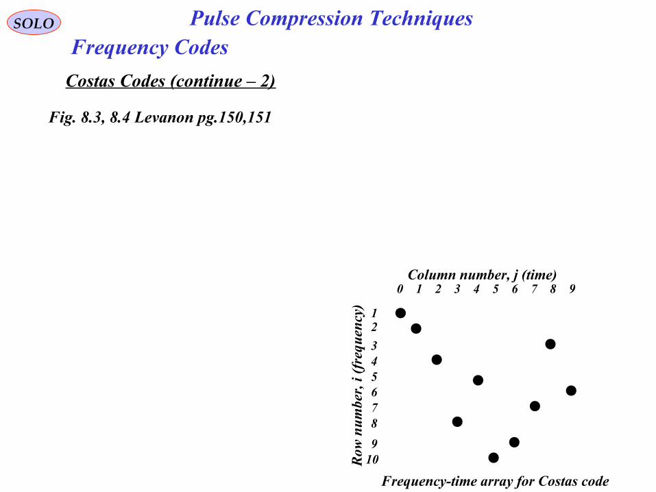
SOLO Pulse Compression TechniquesFrequency Codes
Costas Codes (continue – 2)
0 1 2 3 4 5 6 7 8 9
12
345678
910
Column number, j (time)
Row
nu
mbe
r, i
(fre
quen
cy)
Frequency-time array for Costas code
Fig. 8.3, 8.4 Levanon pg.150,151

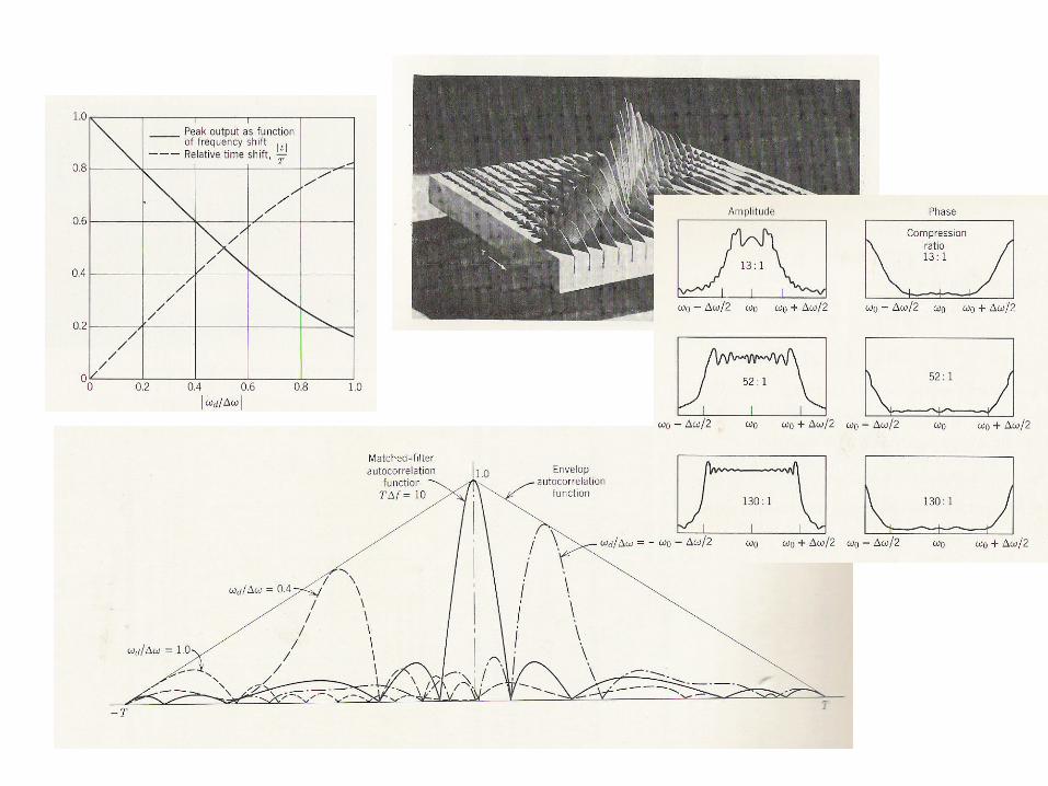
SOLO Pulse Compression TechniquesFrequency Codes
Costas Codes (continue – 3)
• All side-lobes, except for few around the origin, have amplitude 1/N. Few side-lobes close to the origin have amplitude 2/N, which is typical to Costas codes.
• The compression ratio of Costas codes is approximately N.
• The ambiguity function of Costas codes is approaching the ideal thumbtack shape..
• Costas codes have low sensitivity to coherence requirements.
Return to Table of Content

SOLO Pulse Compression TechniquesComplementary Pulse Codes
Complementary codes consist of a pair of codes with complementaryside-lobes, that is, their side-lobes are equal and opposite Golay, 1961).

SOLO

Bogler, P.L., “Radar Principles with Applications to Tracking Systems”, John Wiley & Sons, 1989
References
SOLO Pulse Compression Techniques
Levanon, N., “Radar Principles”, John Wiley & Sons, 1988
Mahafza, B.R., “Radar System Analysis and Design Using MATLAB”, Chapman & Hall/CRC, 2000
Nathanson, F.E., “Radar Design Principles”, McGraw-Hill, 1969
Morris, G.V., “Airborne Pulse Radar”, Artech House, 1988
Berkowitz, R.S. Ed., “Modern Radar – Analysis, Evaluation, and System Design”, John Wiley & Sons, 1965
Richards, M.A., “Fundamentals of Radar Signal Processing”, Georgia Tech Course ECE 6272, Spring 2000
“Principles of Modern Radar” Georgia Tech, 2004, Jim Scheer,
“Advanced Radar Waveforms”Hermelin, S., “Matched Filters and Ambiguity Functions for RADAR Signals”,
Power Point PresentationReturn to Table of Content

January 20, 2015 62
SOLO
TechnionIsraeli Institute of Technology
1964 – 1968 BSc EE1968 – 1971 MSc EE
Israeli Air Force1970 – 1974
RAFAELIsraeli Armament Development Authority
1974 – 2013
Stanford University1983 – 1986 PhD AA

SOLO Fourier Transform of a Signal
The Fourier transform of a signal f (t) can be written as:
A sufficient (but not necessary) condition for theexistence of the Fourier Transform is:
( ) ( ) ∞<= ∫∫∞
∞−
∞
∞−
ωωπ
djFdttf22
2
1
JEAN FOURIER1768-1830
( ) ( )∫+∞
∞−
−= ωωπ
ω dejFj
tf tj
2
1
The Inverse Fourier transform of F (j ω) is given by:
( ) ( )∫+∞
∞−
= dtetfjF tjωω

( ) ( )∫+∞
∞−
−= ωωπ
ω dejFj
tf tj
2
1
Signal
(1) C.W.
( )2
cos00
0
tjtj eeAtAtf
ωω
ω−+==
0ω - carrier frequency
Frequency
( ) ( )∫+∞
∞−
= dtetfjF tjωωFourier Transform
( ) ( ) ( )00 22ωωδωωδω ++−= AA
jFFourier Transform
SOLO Fourier Transform of a Signal

( ) ( )∫+∞
∞−
−= ωωπ
ω dejFj
tf tj
2
1
Signal
(2) Single Pulse
( )
>≤≤−
=2/0
2/2/
τττ
t
tAtf
τ - pulse width
Frequency
( ) ( )∫+∞
∞−
= dtetfjF tjωωFourier Transform
( ) ( ) ( )( )2/
2/sin2/
2/ τωτωτω
τ
τ
ω AdteAjF tj == ∫−
Fourier Transform
SOLO Fourier Transform of a Signal

( ) ( )∫+∞
∞−
−= ωωπ
ω dejFj
tf tj
2
1
Signal
( ) ( )
>≤≤−
=2/0
2/2/cos 0
τττω
t
ttAtf
τ - pulse width
Frequency
( ) ( )∫+∞
∞−
= dtetfjF tjωωFourier Transform
( ) ( )
( )
( )
( )
( )
−
−
++
+
=
= ∫−
2
2sin
2
2sin
2
cos
0
0
0
0
2/
2/
0
τωω
τωω
τωω
τωωτ
ωωτ
τ
ω
A
dtetAjF tjFourier Transform
0ω - carrier frequency
(3) Single Pulse Modulated at a frequency
0ω
ω
( )ωjF
0
τπω 2
0 +
2
τA
0ω
τπω 2
0 −τπω 2
0 +−
2
τA
0ω−
τπω 2
0 −−
τπω 2
20 +τπω 2
20 −
SOLO Fourier Transform of a Signal

( ) ( )∫+∞
∞−
−= ωωπ
ω dejFj
tf tj
2
1
Signal
( ) ( )
±±=>−≤−≤−+
=,2,1,0,2/0
2/2/cos 0
kkkTt
kTttAtf
rand
τττϕω
τ - pulse width
Frequency
( ) ( )∫+∞
∞−
= dtetfjF tjωωFourier Transform
( ) ( )
( )
( )
( )
( )
−
−
++
+
=
= ∫−
2
2sin
2
2sin
2
cos
0
0
0
0
2/
2/
0
τωω
τωω
τωω
τωωτ
ωωτ
τ
ω
A
dtetAjF tj
Fourier Transform
0ω - carrier frequency
(4) Train of Noncoherent Pulses (random starting pulses), modulated at a frequency 0ω
T - Pulse repetition interval (PRI)
SOLO Fourier Transform of a Signal
( ) ( )∫+∞
∞−
−= ωωπ
ω dejFj
tf tj
2
1
Signal
( ) ( )
( ) ( )( ) ( )( )[ ]
−++
+=
±±=>−≤−≤−
=
∑∞
=1000
0
coscos
2
2sin
cos
,2,1,0,2/0
2/2/cos
nPRPR
PR
PRseriesFourier
tntnn
n
tT
A
kkkTt
kTttAtf
ωωωωτω
τω
ωτ
τττω
τ - pulse width
Frequency
( ) ( )∫+∞
∞−
= dtetfjF tjωωFourier Transform
Fourier Transform
0ω - carrier frequency
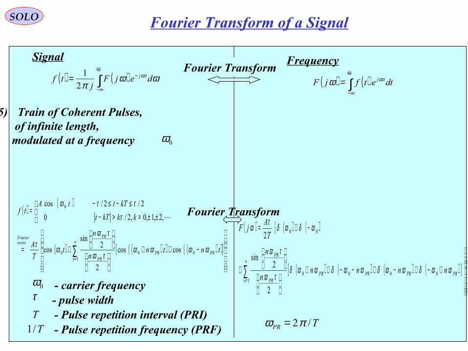
(5) Train of Coherent Pulses, of infinite length, modulated at a frequency 0ω
T - Pulse repetition interval (PRI)
( ) ( ) ( ){
( ) ( ) ( ) ( )[ ]
+−+−+−−++
+
−+=
∑∞
= 10000
00
2
2sin
2
nPRPRPRPR
PR
PR
nnnnn
n
T
AjF
ωωδωωδωωδωωδτω
τω
ωδωδτω
T/1 - Pulse repetition frequency (PRF)TPR /2πω =
SOLO Fourier Transform of a Signal

( ) ( )∫+∞
∞−
−= ωωπ
ω dejFj
tf tj
2
1
Signal
( ) ( )
( ) ( )( ) ( )( )[ ]
−++
+=
±±=>−≤−≤−
=
∑∞
=
≤≤−
1000
22
0
coscos
2
2sin
cos
2/,,2,1,0,2/0
2/2/cos
nPRPR
PR
PRNTt
NT
tntnn
n
tT
A
NkkkTt
kTttAtf
ωωωωτω
τω
ωτ
τττω
τ - pulse width
Frequency
( ) ( )∫+∞
∞−
= dtetfjF tjωωFourier Transform
Fourier Transform
0ω - carrier frequency
(6) Train of Coherent Pulses, of finite length N T, modulated at a frequency 0ω
T - Pulse repetition interval (PRI)
( )( )
( )
( )
( )
( )
( )
( )
( )
( )
( )
( )
( )
−−
−−
++−
+−
++
+
+
−+
−+
+++
++
++
+
=
∑
∑
∞
=
∞
=
10
0
0
0
0
0
10
0
0
0
0
0
2
2sin
2
2sin
2
2sin
2
2sin
2
2sin
2
2sin
2
2sin
2
2sin
2
nPR
PR
PR
PR
PR
PR
nPR
PR
PR
PR
PR
PR
TNn
TNn
TNn
TNn
n
n
TN
TN
TNn
TNn
TNn
TNn
n
n
TN
TN
T
AjF
ωωω
ωωω
ωωω
ωωω
τω
τω
ωω
ωω
ωωω
ωωω
ωωω
ωωω
τω
τω
ωω
ωωτω
T/1 - Pulse repetition frequency (PRF)TPR /2πω =
SOLO Fourier Transform of a Signal

Signal
( ) ( )
+=
±±=>−≤−≤−
= ∑∞
=11 cos
2
2sin
21,2,1,0,2/0
2/2/
nPR
PR
PRSeriesFourier
tnn
n
T
AkkkTt
kTtAtf ω
τω
τωτ
τττ
τ - pulse width0ω - carrier frequency
(6) Train of Coherent Pulses, of finite length N T, modulated at a frequency 0ω
T - Pulse repetition interval (PRI)
T/1 - Pulse repetition frequency (PRF)TPR /2πω =
( ) ( )tAtf 03 cos ω=
t
A A
( )tf1
t
2
τ2
τ−T
A
T T
22
τ+T2
2τ−T
T T
2
τ− 2
τ+T
( )tf 2
t
TN
2/TN2/TN−
( ) ( ) ( ) ( )tftftftf 321 ⋅⋅=
( ) ( ) ( ) ( ) ( )
( ) ( )( ) ( )( )[ ]
−++
+=
±±=>−≤−≤−
=⋅⋅=
∑∞
=
≤≤−
1000
22
0
321
coscos
2
2sin
cos
2/,,2,1,0,2/0
2/2/cos
nPRPR
PR
PRNTt
NT
tntnn
n
tT
A
NkkkTt
kTttAtftftftf
ωωωωτω
τω
ωτ
τττω
( )
>≤≤−
=2/0
2/2/12 TNt
TNtTNtf ( ) ( )ttf 03 cos ω=
SOLO Fourier Transform of a Signal