detecting sybil nodes in static and dynamic networks by

Detecting Sybil Nodes in Static and Dynamic Networks

by

Jose Antonio Cardenas-Haro

A Dissertation Presented in Partial Fulfillmentof the Requirements for the Degree

Doctor of Philosophy

Approved November 2010 by theGraduate Supervisory Committee:

Goran Konjevod, Co-ChairAndrea W. Richa Co-Chair

Arunabha SenGuoliang Xue

ARIZONA STATE UNIVERSITY

December 2010

ABSTRACT

Peer-to-peer systems are known to be vulnerable to the Sybil attack. The lack

of a central authority allows a malicious user to create many fake identities (called

Sybil nodes) pretending to be independent honest nodes. The goal of the malicious

user is to influence the system on his/her behalf. In order to detect the Sybil nodes

and prevent the attack, a reputation system is used for the nodes, built through

observing its interactions with its peers. The construction makes every node a part

of a distributed authority that keeps records on the reputation and behavior of the

nodes. Records of interactions between nodes are broadcast by the interacting nodes

and honest reporting proves to be a Nash Equilibrium for correct (non-Sybil) nodes.

In this research is argued that in realistic communication schedule scenarios, simple

graph-theoretic queries such as the computation of Strongly Connected Components

and Densest Subgraphs, help in exposing those nodes most likely to be Sybil, which

are then proved to be Sybil or not through a direct test executed by some peers.

i

To Beatriz and Sofıa

ii

ACKNOWLEDGMENTS

I want to express my gratitude to Dr Goran Konjevod for all his support in my

research; he has been not only great advisor but also a good friend. Special thanks

to Dr Richa, Dr Sen and Dr Xue for their aid and good questions that helped me

through my research problems.

My recognition to all my friends at the lab that made me feel very confortable

among them. Also my gratitude and love to my wife for her patience and backing

on my graduate studies, and to my beautiful daughter that charms our life.

My thankfulness to the Fulbright and Conacyt programs, without the funding from

them this achievement would not have been possible.

Note: The algorithms presented in this thesis were partly described in the paper

Detecting Sybil Nodes in Static and Dynamic Networks, presented at OTM 2010 and

published in LNCS by Springer [6].

iii

TABLE OF CONTENTS

Page

LIST OF TABLES . . . . . . . . . . . . . . . . . . . . . . . . . . . . . . . . . vi

LIST OF FIGURES . . . . . . . . . . . . . . . . . . . . . . . . . . . . . . . . vii

LIST OF ALGORITHMS . . . . . . . . . . . . . . . . . . . . . . . . . . . . . ix

CHAPTER 1 INTRODUCTION . . . . . . . . . . . . . . . . . . . . . . . . 1

1.1. Introduction . . . . . . . . . . . . . . . . . . . . . . . . . . . . . . . . 1

1.1.1. Existing work . . . . . . . . . . . . . . . . . . . . . . . . . . . 1

1.1.2. Discussion . . . . . . . . . . . . . . . . . . . . . . . . . . . . . 6

1.2. Background . . . . . . . . . . . . . . . . . . . . . . . . . . . . . . . . 7

1.2.1. Strictly proper scoring rule . . . . . . . . . . . . . . . . . . . . 7

1.2.2. Strict Nash equilibrium . . . . . . . . . . . . . . . . . . . . . . 7

1.2.3. Stochastically relevant . . . . . . . . . . . . . . . . . . . . . . 8

1.2.4. Strongly connected component . . . . . . . . . . . . . . . . . . 8

1.2.5. Clique . . . . . . . . . . . . . . . . . . . . . . . . . . . . . . . 8

CHAPTER 2 MODEL AND BASIC OBSERVATIONS . . . . . . . . . . . . 9

2.1. Model and assumptions . . . . . . . . . . . . . . . . . . . . . . . . . . 9

2.2. General observations . . . . . . . . . . . . . . . . . . . . . . . . . . . 11

2.3. System Model . . . . . . . . . . . . . . . . . . . . . . . . . . . . . . . 14

CHAPTER 3 GOALS AND PROBLEM STATEMENT . . . . . . . . . . . 16

3.1. The anonymity issue . . . . . . . . . . . . . . . . . . . . . . . . . . . 16

3.2. Static and dynamic settings . . . . . . . . . . . . . . . . . . . . . . . 16

3.3. Dealing with multiple Sybil groups . . . . . . . . . . . . . . . . . . . 17

3.4. Distinguishability errors . . . . . . . . . . . . . . . . . . . . . . . . . 17

iv

4.1. Collusion among Sybil groups . . . . . . . . . . . . . . . . . . 19

3.4.2. Formal observers . . . . . . . . . . . . . . . . . . . . . . . . . 19

CHAPTER 4 THE ALGORITHM . . . . . . . . . . . . . . . . . . . . . . . 21

4.1. Overview . . . . . . . . . . . . . . . . . . . . . . . . . . . . . . . . . . 21

4.2. Temporal Coincidences . . . . . . . . . . . . . . . . . . . . . . . . . . 23

4.3. Game Theory and the Reputation System . . . . . . . . . . . . . . . 24

4.4. Matrices Built . . . . . . . . . . . . . . . . . . . . . . . . . . . . . . . 27

4.4.1. Reputation Matrix . . . . . . . . . . . . . . . . . . . . . . . . 28

4.4.2. Counter Matrix . . . . . . . . . . . . . . . . . . . . . . . . . . 28

4.4.3. Inbucket Matrix . . . . . . . . . . . . . . . . . . . . . . . . . . 33

4.5. Report Broadcasting and the Time Buckets . . . . . . . . . . . . . . 36

4.6. Finding the Strongly Connected Components . . . . . . . . . . . . . 42

4.7. Finding Densest Subgraphs . . . . . . . . . . . . . . . . . . . . . . . 44

4.8. Tests on Suspicious Nodes . . . . . . . . . . . . . . . . . . . . . . . . 47

4.9. The Algorithm to detect the Sybil nodes . . . . . . . . . . . . . . . . 48

4.10. The Running Time . . . . . . . . . . . . . . . . . . . . . . . . . . . . 51

CHAPTER 5 SIMULATION RESULTS . . . . . . . . . . . . . . . . . . . . 53

5.1. Detection by Strongly Connected Components . . . . . . . . . . . . . 53

5.2. Detection by Densest Subgraphs . . . . . . . . . . . . . . . . . . . . . 57

CHAPTER 6 CONCLUDING REMARKS AND FUTURE WORK . . . . . 62

6.1. Conclusions . . . . . . . . . . . . . . . . . . . . . . . . . . . . . . . . 62

REFERENCES . . . . . . . . . . . . . . . . . . . . . . . . . . . . . . . . . . . 64

v

LIST OF TABLES

Table Page

1. Payout Rules . . . . . . . . . . . . . . . . . . . . . . . . . . . . . . . 25

2. Time buckets for the reputation matrix example . . . . . . . . . . . . 30

3. The reputation matrix after the first time bucket from table 2 . . . . . 30

4. The reputation matrix after the fifth time bucket from table 2 . . . . 32

5. Time buckets for the counter matrix example . . . . . . . . . . . . . . 32

6. The counter matrix after the first time bucket from table 5 . . . . . . 33

7. The counter matrix after the fifth time bucket from table 5 . . . . . . 35

8. Time buckets for the Inbucket Matrix example . . . . . . . . . . . . . 35

9. The inbucket matrix after the first time bucket from table 8 . . . . . . 36

10. The inbucket matrix after the fifth time bucket from Table 8 . . . . . 37

11. Inbucket Matrix after the first time bucket . . . . . . . . . . . . . . . 41

12. Nonlinear Model Results . . . . . . . . . . . . . . . . . . . . . . . . . 42

13. Example of connections among nodes. . . . . . . . . . . . . . . . . . . 61

vi

LIST OF FIGURES

Figure Page

1. A Sybil couple (η10 and η14) broadcasting reports along with pairs of

regular nodes within the same time bucket. . . . . . . . . . . . . . . . 39

2. Detection results by the Strongly Connected Components method for

every one hundred experiments with 5% and 10% of Sybil nodes re-

spectively. . . . . . . . . . . . . . . . . . . . . . . . . . . . . . . . . 53

3. Sybil nodes simulating an interaction with their Sybil peer a, in order

to boost their reputation points. . . . . . . . . . . . . . . . . . . . . . 55

4. Detection results through the Strongly Connected Components method

for every one hundred experiments with 15% and 20% of Sybil nodes

respectively. . . . . . . . . . . . . . . . . . . . . . . . . . . . . . . . . 56

5. Detection results by the Strongly Connected Components method in

the cases of 5% and 10% of Sybil nodes situation. The “x” axis repre-

sents the time buckets. . . . . . . . . . . . . . . . . . . . . . . . . . . 57


the cases of 15% and 20% of Sybil nodes situation. The “x” axis

represents the time buckets. . . . . . . . . . . . . . . . . . . . . . . . 58


the cases of 10%, 15% and 20% of Sybil nodes situation. The “x” axis

represents the time buckets. . . . . . . . . . . . . . . . . . . . . . . . 59

8. Detection results by the Densest Subgraph method in the presence of

different percentages of Sybil nodes. . . . . . . . . . . . . . . . . . . 60

vii

Figure Page

9. Detection results by the Densest Subgraph method in the cases of 5%,

10%, 15% and 20% of Sybil nodes environment. The “x” axis repre-

sents the time buckets. . . . . . . . . . . . . . . . . . . . . . . . . . . 60

viii

LIST OF ALGORITHMS

Algorithm Page

1 Building the Reputation Matrix . . . . . . . . . . . . . . . . . . . . . . 29

2 Building the Counter Matrix . . . . . . . . . . . . . . . . . . . . . . . 31

3 Building the Inbucket Matrix . . . . . . . . . . . . . . . . . . . . . . . 34

4 Interaction and creation of reports for broadcast . . . . . . . . . . . . 38

5 Detecting the Sybil groups by Strongly Connected Components . . . . 45

6 Detecting the Sybil groups by Densest Subgraphs . . . . . . . . . . . . 48

7 Testing the nodes to corroborate the Sybilness . . . . . . . . . . . . . 49

8 The complete process of detecting the Sybil nodes . . . . . . . . . . . 52

ix

CHAPTER 1

INTRODUCTION

1.1 Introduction

In a large distributed network system, many types of security threats arise. A number

of these are due to weaknesses in cryptographic protocols and concern the detection

of malicious users trying to access data they do not have the rights to access, or

forging another user’s identity. Unlike those problems, Sybil attack is closely linked

to the level of anonymity allowed by the system. Many security mechanisms, voting

and recommendation systems base their protocols on the assumption of a one-to-one

correspondence between entities and identities. If this basic assumption is broken,

those systems are compromised. Sybil attack denotes the creation of many (fake)

identities by a single entity in a distributed system, for the purpose of influencing

and disrupting the normal behavior of the system.

1.1.1 Existing work

Sybil attack was first named and studied by Douceur [10]. Douceur used the “com-

munication cloud” model of communication, where a node “submits” a (possibly

encrypted) message into the cloud, and any node capable of reading the message

may do so by simply “plucking it out” of the cloud and decrypting it if necessary.

The point of stating the model this way was not so much the broadcast nature of it,

but the fact that the origin of a message may only be determined from the message

contents, and not from any network-provided information on the message (headers,

or the actual host/router from which the message was received). In other words, the

identity of a message sender cannot be determined from any external information

about the message, only from the message contents. Douceur proved that Sybil

1

attack cannot be prevented in such a model, and its severity only depends on the

computational power of the malicious user relative to the computational power of

honest users. Basically, as long as there is no centralized authority that would cer-

tify identities of users accepted into the network, the number of identities an entity

may create is only limited by the amount of work the entity puts into this activity.

(The removal of typical communication infrastructure from the model may also be

motivated by thinking of this infrastructure as equivalent to a centralized identity-

verification authority). Since the paper of Douceur [10], many others papers have

been published on various forms of the Sybil attack problem [14] [18] [20] [2] [4] [5]

[23] [22] [12].

Newsome et al. [14] studied the problem in the context of sensor networks and

their methods were designed to work with the specific properties of radio resources,

for example, they assumed that a node may not listen simultaneously on more than

one frequency. Sastry et al. [18] presented an early version of a protocol that verifies

node locations and bases node identities on their location information. Similar ideas

were also proposed by Waters and Felten [20], Bazzi and Konjevod [2] and Capkun

and Hubaux [4, 5]. In the most general form, these works are based on measuring

the delays incurred by communications between nodes and imposing a geometric

structure on the “distance space” to determine node locations. In particular, Bazzi

and Konjevod show that, assuming the triangle inequality and a geometry close

to Euclidean, even in the presence of colluding malicious users, one can design

distributed protocols to localize nodes and thus help prevent Sybil attack. The

common fundamental assumption here is that each real entity has the additional

2

property of physical location within the distributed system, and that this property

will influence the communication by the entity sufficiently that a powerful enough

observer may distinguish it from the communication by any other entity. (Even if it

is not always the case that every pair of entities may be distinguished, if the groups

of indistinguishable entities are small enough, most of the repercussions of a Sybil

attack may be prevented.)

The disadvantage of relying on the geometry of roundtrip delays is that it

applies only to systems with honest routers. Also, due to the variability of network

load and delays it is not always possible to have accurate measurements of roundtrip

delays and clock synchronizations between routers that can be far apart physically.

Another inconvenience is when a malicious user controls several network locations.

In such condition the attacker can fabricate arbitrary network coordinates between

those locations, thus breaking the proposed security system. Furthermore, this

system would not work at all in a dynamic network. On the other hand, this work

does describe remotely issued certificates that can be used to test the distinctness

of identities, and that idea may be of use combined with some facets of our approach.

More recently, Yu et al. [23, 22] gave protocols that rely on a different

restriction: they assume the existence of “secure” links between, say, pairs of

friends in the network. Thus, any message coming directly through such a link

comes with a known origin. In other words, one recognizes that the message was

sent by a good friend (although, if the message is only relayed by the friend, no

3

more is known about its origin). This may be seen as a step towards allowing

centralized infrastructure, but the local nature of the edges encourages us to

think about them as “local authorities”. In order to “set up” these edges, Yu

et al. assume prior “out-of-band” communication. They also assume that the

network formed by these edges is fast-mixing, which they claim to be the case for

most social networks. Finally, they notice a different type of restriction that is

naturally present at Sybil nodes. Since a malicious node that creates many Sybil

identities is only one node, not only is its computational power limited, but so

is its bandwidth. In short, Yu et al. require a node applying for acceptance to

the system to send a message that performs an “almost random” walk. The node

receiving the application (“the verifier”) does the same. Then, if two messages

cross paths, the node is accepted. The idea behind their argument is that Sybil re-

gions are bandwidth-limited and a message sent from within one will rarely “escape”.

In both SybilGuard [23] and SybilLimit [22], the protocol is based on the “social

network” among user identities, where an edge between two identities indicates an

established trust relationship between two humans. The edge key distribution is

done out-of-band which is a disadvantage in most cases. The protocols will not

work if the adversary compromises a large fraction of the nodes in the system.

An assumption on which both SybilGuard and SybilLimit rely is that malicious

users may create many nodes but relatively few attack edges. This is partially true

since these protocols are more effective in defending against malicious users than

in defending against compromised honest users that already belong to the system.

4

This is because a malicious user must make real friends in order to increase the

number of attack edges, while compromised honest users already have friends. These

protocols also break the anonymity of users, which is impractical in most cases since

anonymity for many peer-to-peer users is a high priority. Taking away anonymity

will prevent many users from participation.

Lesniewski-Laas [12] assumes a one hop distributed hash table which uses the

social links between users to resist the Sybil attack. As in the case of SybilGuard and

SybilLimit, he bases his protocols in human established trust relationships breaking

the anonymity of users. This is similarly difficult to apply to real-life networks

since many users in peer-to-peer systems prioritize anonymity as a condition of

participation. Furthermore, a one-hop distributed hash table (DHT) is not a realistic

approach for the World Wide Web. Users may be many hops apart, breaking the

assumptions of the protocol proposed by Lesniewski-Laas [12].

Piro et al. [16] study Sybil attack in mobile ad-hoc networks, and propose some

protocols we find interesting. The simple observation made by them (that we are

not aware of having appeared in the literature before) is that Sybil nodes are tied

to their “maker”, and that this has special consequences in a mobile network. That

is, identities from a Sybil group that was constructed by a single malicious user

will never appear simultaneously in different regions of the network. So, if nodes

have limited capabilities of observation and if two nodes who know they are far

apart observe two identities roughly simultaneously, then these two identities are

5

certainly not part of the same Sybil group. On the flip side, if two identities are

always seen together over a long period of time, then there should be a reason for

that. Unless they are linked by some other mechanism, they are very likely Sybil

identities. Remarkably, this intuition, while it appears key in the mobile setting, is

of little use in the static case. Thus, it forms a complement to the location-and-delay

based certification mechanisms of Bazzi and Konjevod [2] which were limited to the

static setting. In fact, the basic observation that a pair of independent users of a

mobile ad-hoc network will frequently be seen simultaneously in different locations

in the network, while a Sybil node is never seen far from its “master”, forms the

foundation for this research as well. However, we believe our approach is simpler and

at the same time requires fewer additional assumptions.

Piro et al. [16] also propose monitoring of the network traffic and the collisions

at the MAC level. The limitation in this case is that this only works for mobile ad

hoc networks. Others [1] propose resource testing to discourage rather than prevent

Sybil attacks.

1.1.2 Discussion

What all of these existing approaches have in common is that they restrict the origi-

nal problem formulation by making assumptions that allow the distributed system to

enforce stronger limitations on the creation of fake identities. Usually, these assump-

tions are justified by arguments about physical properties of any real peer-to-peer

network that restrict the communication cloud model by requiring some form of cost

to be associated with each interaction between peers, either time taken by a message

to reach its recipient(s), or bandwidth required for the message, or cost paid by an

6

entity to have the message processed. This observation motivates our work by in-

dicating that a distributed mechanism (in which all correct nodes participate) that

imposes a certain type of cost on each communication step may in fact sufficiently

emulate the implications of the existence of a centralized authority that Sybil attack

becomes much harder in the system that employs such a mechanism.

1.2 Background

It is relevant to explain here some of the terms used in this thesis for the best

assimilation of Chapter 4.

1.2.1 Strictly proper scoring rule

A scoring rule or scoring function is used in decision theory to know the efficiency

of decision takers under conditions of uncertainty. It is called “proper” when it has

been optimized for some set of conditions, and it is called “strictly proper” if it has

been uniquely maximized for a very specific case [11][13].

1.2.2 Strict Nash equilibrium

Nash equilibrium is a term used in game theory to define a set of rules to specify an

equilibrium between two or more players competing against them, considering that

every player know the equilibrium strategies of the others, and no one can improve

the gain doing unilateral changes in its strategy.

In general, it is said that a strict Nash equilibrium is present when the strategy used

by every player is the best, given the strategies used by its peers. In other words, no

other combination of strategies between the players can improve the gains [13][15].

7

1.2.3 Stochastically relevant

Let X and Y be two random variables. It is said that X is stochastically relevant for

Y only if the distribution of Y conditional on X is not equal for different realizations

of X; i.e. Pr(y|x) 6= Pr(y|x′) where x and x′ are different realizations of X, and y

is a realization of Y . In the context of probability and statistics, a realization is the

value observed in a random variable under certain conditions [13][21].

1.2.4 Strongly connected component

When there is a path from any node to any other node in a directed graph (or

subgraph), it is said that the nodes in such graph (or subgraph) are forming a strongly

connected component [9].

1.2.5 Clique

When there is an edge between any two nodes in an undirected graph (or subgraph),

it is said that the nodes in such graph (or subgraph) are forming a clique [9]. The

clique problem (finding a clique in a graph) is NP-Complete. An efficient way to

find them is looking for densest subgraphs. An algorithm for that is proposed by

Charikar [7].

8

CHAPTER 2

MODEL AND BASIC OBSERVATIONS

2.1 Model and assumptions

In most of this research is assumed an abstract theoretical network model where the

nodes are in a fully connected topology and the signal of the mobile nodes reach

all their peers. This can be considered in a more abstract way as a local network

topology.

However, the topology of the network ends up being mostly abstracted away

by the communication cloud assumption mentioned earlier: we assume that each

message sent by any node is broadcast into the communication cloud, and the only

information about the origin of a message a node observes in the communication

cloud, (or equivalently, hears by listening) is contained within the contents of the

message. For example, a node cannot tell the source, or even a single network router

from which the message comes from a header, or by examining the message without

reading its contents. Thus, a message may be signed by a node, but the identity

claimed by the signing node cannot be verified directly unless we already know that

node. This assumption is used instead of any specific other about the geometry

(a metric, in particular Euclidean space, was the key to the design of Sybil attack

detection protocols in [2]) or the topology (a fast-mixing network was crucial to

the protocols in [23, 22]). In other words, The physical positions of the nodes are

irrelevant for our algorithm from the local network point of view. On the other

hand, we do assume standard cryptographic protocols such as digital signatures and

public-key cryptography work.

9

Note that, similar to [2], an assumption is made that identifies a property of

a Sybil attacker and its collection of fake identities that, to an observer capable of

surveying all the events in the network, would make it obvious that is something

strange going on there. In the static setting of [2], the observer would notice many

identities at the exact same physical location in the network. In our current dynamic

setting, the image would be even more blatant: the Sybil nodes will appear in-

terconnected in a densest subgraph or in a strongly connected component, or in both.

However, we avoid specific details beyond this general assumption. We are more

interested in the fundamental consequences of anonymity in distributed systems and

in the fundamental obstacles to secure identity management than in special cases,

and so our goal is to study what can be achieved with a minimum set of assumptions

rather than to provide a complete practically working solution for a very specific

existing real world system.

The basic observation made in [16], that two or more identities belonging to the

same malicious user are connected to their master, is instrumental in our work as

well, although we use it in a fundamentally simpler way. Few variants of the more

general problem that were left open until now, are also addressed here, where a

Sybil attacker attempts to thwart the detection process, and uses different subsets of

its identities at different times, or even exchanges its identities with another attacker.

10

2.2 General observations

We begin by noting that Sybil nodes by themselves may not be bad, but the major

reason to create them in the first place is to affect the system at some point in time.

All those nodes under the control of an individual can be used to negatively affect

the system. For example, they can change the outcome of a ballot or influence

the reputation of others. On the other hand, when a Sybil node is not actively

used, it doesn’t really change the system behavior, and so its bare existence is not

necessarily a threat.

Let us analyze here the basic assumptions made in the work of Piro et al. [16]

in order to clarify the differences and analogies with our work. They consider

the network as evolving over a period of time, and, for simplicity, they divide the

timeline into discrete intervals. Then, the role of network “observers” is assigned to

a set of nodes. An observer simply keeps track of nodes it sees in its vicinity over

a sequence of time intervals. Aggregating the data from multiple observers, can be

listed, for every time interval, the nodes observed in various parts of the system.

Since the range of a message is limited, observers that are far away from each

other will observe disjoint subsets of nodes during any given time interval. Thus they

notice and claim the basic fact that underlies their approach: two identities observed

during a single time interval by observers that are far away from each other, belong

to two independent entities. In other words, if an entity and any of its Sybil nodes

are observed simultaneously, they will be observed in regions of the system that are

11

close-by. This approach made by Piro et al. [16] is very specific for mobile ad hoc

networks.

These are the conclusions that may be attempted by (a group of) observers in

that model.

1. Node A is observed by o1 and node B by o2 during the same time interval. The

observers o1 and o2 are far away from each other.

In this situation, it is immediately clear that A and B are identities that belong

to distinct entities, since a single entity could not be visible simultaneously in

several network locations. This event implies that A and B are distinguishable

entities, and the distributed system should in the future be able to rely on this

knowledge.

2. Node A is observed simultaneously with node B by observer o1.

Not so much can be concluded from a single such observation. On the other

hand, it may be reasonable to assume that distinct entities will in fact not

constantly move together and be located near each other. If this is true, then

each time two nodes are observed together, the likelihood that they are not

independent, and that one is a fake identity created by the other, becomes

higher.

3. Node A is observed during a time period when node B is not seen anywhere.

As in the previous case, nothing can be concluded with certainty about those

two nodes from a single observation. The two nodes may be independent, but

this event may also be a consequence of a malicious node trying to hide its tracks

12

by selectively activating subsets of nodes it controls. If one could assume that

distinct entities operate so that the periods in which the entities in a subset are

active are not highly correlated, or are even statistically independent, then the

laws of probability would indicate that two identities such that, at any given

time, at most one is seen anywhere, most likely are two identities associated

with the same entity, and so that at least one of them is a Sybil identity.

However, in some cases, this situation is not as severe: since at most one

of the two identities is seen at any given moment, even if one or both are

fake identities, the damage to the distributed system is likely not very large.

Depending on the actual purpose of the distributed system, this situation may

not be of grave concern.

In a similar way, we use the basic assumptions made by Piro et al. [16] but in

a quite different approach. We do not follow the physical positions of the nodes

through the local network. Instead of physical positions we keep track of the timing

and contents of the reports broadcast by the nodes. With that information we can

infer different relations among the nodes. The weaknesses of the malicious users

and their Sybil nodes will be magnified as the time passes and more information is

gathered about their behavior. Once enough information is collected in the matrices

described in Section 4.4, the Sybil relations can be detected as densest subgraphs or

strongly connected components.

13

2.3 System Model

Our system consists of a set A of k honest nodes, of a set B of m authority nodes

and a set C of n Sybil nodes. The set B is equal to A (in some cases B could be just

a subset of A). The set A ∪ B ∪ C is the set of participants. In some problems, we

assume the participants are points in either the standard d-dimensional Euclidean

space Rd or the d-dimensional unit sphere S

d. In making statements that hold for

both Rd and S

d, we refer to the space as X. We also assume that some participants

are mobile and that others have fixed positions. The distance between the nodes x

and y in X is denoted by ρ and that distance might change over time if at least one

of those nodes is mobile. We analyze the behavior of the nodes in X by dividing

the time into slots and we consider all the nodes as static for any particular slot. In

our system model we also assume a synchronized clock for all the network. In real

systems this could be the Unix time proposed by Ritchie and Thompson [17].

Ideally all the honest nodes are authority nodes (or observers) and they are

constantly listening the network for information signals (reports) to fill out their own

matrices. Theoretically in our model all the honest nodes have the same information

in their matrices, so all of them will end up finding the same densest subgraphs

and strongly connected components. In order to avoid flooding the network with so

many broadcasting, just some nodes can be set as authorities. Such selection can be

done based on the reputation and antiquity of the nodes (the lower indexes indicate

more antiquity). Any node detected or suspected of being Sybil cannot be trusted

as authority node and has to be substituted by another.

14

In the event that only few nodes are set as authorities, they have to maintain an

information pool accessible to all. In the case of several local networks interconnected,

some issues arise. The information in the matrices could not be homogeneous for all

the nodes and the results will mismatch. In this case, the authority nodes of different

local networks will work more like the observer nodes proposed by Piro et al. [16].

15

CHAPTER 3

GOALS AND PROBLEM STATEMENT

To summarize our discussion so far, given in the previous Chapters, here is a list of

desirable properties for an approach to the Sybil attack problem that would improve

on the current state of knowledge.

3.1 The anonymity issue

An issue is the anonymity of users (which is endangered in the presence of a central

certificate authority) versus their safety against Sybil attacks.

It is not always possible to use certificate authorities to guarantee that each per-

son has only one identity. Good certifying agencies are expensive and may discourage

the participation of many users. In other cases, the users would prioritize anonymity,

for example in forums about religion, sex, politics, family violence, etc.

In other words, we need a self-policing peer-to-peer system that allows users to keep

their anonymity.

3.2 Static and dynamic settings

Existing solutions against Sybil attack work in special network models. Furthermore,

each of them assumes either a completely static or a very dynamic topology.

The other issue here is that in the real world the users are a mixture of mobile

and static nodes. So far, the proposed approaches work only exclusively in static

or mobile networks, but not in both. There is a lack of an algorithm that works to

validate static and mobile users as well. In the absence of a certifying authority, the

rules and policies used have to be defined and enforced by the peers themselves. Our

solution works in mobile and static nodes, or in a mixture of them as well.

16

3.3 Dealing with multiple Sybil groups

The existence of multiple malicious users is a major unsolved problem related to

Sybil attack. By unsolved, we mean here that practically no proposed approach to

dealing with Sybil attack offers any relief in the situation where several malicious

users create independent Sybil groups, even if they act independently and do not

collude to make each other’s behavior more difficult to detect.

We argue that our solution works well even in the presence of multiple malicious

users, as long as they are not colluding. With several, or many attackers working

as a team handling together the same group of Sybil nodes, they can camouflage

even more the Sybil nodes making them appear “more normal” in their behavior and

making their detection harder.

3.4 Distinguishability errors

How can a protocol based on the ideas described in Section 2.2 fail? The main

action performed is to conclude that two identities are distinguishable when they

are reported to be present in two different locations simultaneously. Now, suppose

two identities A and B are pronounced distinguishable when they are in fact two

Sybil identities controlled by the same entity. First, the mode in which nodes of

the network lie is not such that nodes simply lie about having seen one of the two

identities. If the reports about having seen A and B really do come from two regions

of the network that are sufficiently far away, then the nodes reporting this cannot

be controlled by a single entity.

17

In fact, thus we see that if A and B are falsely pronounced distinguishable, then

some node participating in this must be lying about its location in the network: only

if a node claims to be farther away from its Sybil siblings, can its claim of having

seen A at the same time as the rest of the nodes saw B be taken as evidence of

distinguishability for A and B. Suppose X claims to have seen A and Y to have seen

B, while X and Y were far away from each other. Now, either X or Y is lying about

its own location. Since the Sybil siblings of X and Y are restricted to one of the two

locations, say the location of X, we may conclude that Y ’s lie will be exposed as

soon as one consults any node who really was where Y claims to have been at the time.

If we refer to an error such as described above as a false positive (two identities

falsely distinguished), what about a false negative? This means two identities are

never pronounced distinguishable while they are actually two separate entities. As

argued above, except for special circumstances, this should be a very rare event.

Piro et al. [16] suggest that one may detect this by examining the amount of traffic

within such a group of mutually indistinguishable nodes.

Namely, the amount of traffic should be proportional to the square of the number

of nodes in the group if these are distinct entities, while it will be much smaller (linear

in this number) in a Sybil group: whenever Sybil node A communicates with Sybil

node B, the Sybil master is the one actually working the communication channel on

both ends.

18

3.4.1 Collusion among Sybil groups

We have argued that a false positive is not easy to achieve for a single malicious

adversary. However, if two entities controlling Sybil groups collude, the detection

problem becomes more difficult. Consider two nodes A and B, each controlling a

Sybil group. In order to help A cheat and pass off its Sybil nodes a1 and a2 as

distinguishable, B (located sufficiently far away from A) claims (through any of its

Sybil nodes) to have seen a2 at the same time that A claims (through any of its

Sybil nodes) to have seen a1. Now, if there are no honest nodes located close enough

to B’s position to be able to observe a2 where B claims to have seen it, there is not

much that can be done. However, if there are, there will be a discrepancy between

their reports and those of B.

In this situation, in fact, it appears that one must require that there are more

honest nodes than the Sybil nodes controlled by B in the area where they would

observe a2. Then when it comes to examining their reports on observed nodes, more

nodes will vote not to have seen a2 than to have seen it, and the system will correctly

conclude that a2 could not have been in the area.

3.4.2 Formal observers

Having sketched out the generalities, we describe more precisely a possible approach

to more precise implementation of the ideas. As in some other proposed strategies to

defeat Sybil attack, one could maintain a set of nodes formally authorized to work

as a group and issue credentials for accessing the network. Of course, there will be a

need to enforce the correctness of their behavior, for example, to prevent them from

19

defection and sudden turn to working with a Sybil group. This can be achieved, for

example, by duplicating the system and thus reducing the chance of corruption.

But let us describe the role of these “observers”. They are relatively static in

the network and they relinquish their roles when they move, handing off to new

members of the group. They cover all the regions of the network and maintain a

connected overlay that has members close enough to “every corner” so they can

observe and confirm any claimed location of a node in the network. They may work

similarly to “beacons” in [2], establishing protocols by which new applicants to

the network and those who have just moved are issued and reissued access credentials.

A few corrupt observers will not break the system in general, but strategically

selected ones may cause some serious damage and so we envision these nodes as

running distributed protocols resilient to failure of a small subset of nodes.

20

CHAPTER 4

THE ALGORITHM

4.1 Overview

Our basic solution has two major components: a reputation system based on the

outcomes of interactions between peers in the network, and a separate analysis of

interactions according to their participants’ locations in time and space.

We consider the Sybil nodes as being under the control of an adversary which

may be one or more malicious users, colluding or not. Honest nodes participate in

the system to provide and receive service as peers. Honest nodes need a mechanism

to detect Sybil nodes and protect themselves against the Sybil attack. Ideally, the

mechanism of detection should be efficient enough to detect the Sybil nodes before

they gain enough reputation as trustable. The nodes are not restricted in any way

to participate in P2P operations and they can build a reputation over time that

will make them trustable. The nodes earn reputation points using a game-theoretic

mechanism. In our approach, after interacting with a peer, each node must (locally)

broadcast a report on the outcome of such interaction. Any nearby authority nodes

are always listening for those reports and collecting information on the fly. Such

information is later used to infer Sybil relations between nodes. Part of this research

has been published at the LNCS [6].

At a high level, every interaction between two nodes results in summary reports

of the interaction made by both participants. These reports contribute to reputation

scores, but they are also used to create a graph (where the edges link nodes who

are rating other nodes) whose connectivity structure is analyzed. Since a pair of

21

reports is created solely by the pair of nodes reporting on their interaction, two

Sybil nodes might falsify a large number of reports in order to boost each other’s

reputation. However, if overused, this will become obvious through an analysis of

the rating graph. The third mechanism we use to detect Sybil candidates is based

on the observation that independent nodes tend to behave independently, both in

terms of where they are located, and in terms of when they communicate.

It is worth noticing here that we never restrict in any way a node from

participating and interacting with its peers (unlike some earlier systems where a

node would have to be certified before it was admitted to the network). We consider

each node honest until proven otherwise; however, if a node does not have enough

reputation points, it will not be considered very trustworthy and subsequently it

will not be able to cause much damage.

When the interaction between any two peers is over, both nodes perform a

(local) broadcast of their reports on that interaction. These two reports must match,

otherwise those nodes are marked as suspicious. From the reports that have been

broadcast and their timing, every node over time builds three data sets as explained

in Section 4.4. There is always the possibility of pairs of Sybil nodes simulating an

interaction and broadcasting false reports, in order to increase their reputations as

trustworthy nodes. It is possible they may do this infrequently, however if this is

abused, they will expose themselves since after a large number of “interactions” such

as these, there will be enough information to explore the graph induced by such

22

interactions and identify active Sybil groups as its Strongly Connected Components.

For details, see Section 4.6.

Furthermore, from the timing of the report broadcasts we can learn useful in-

formation as well. For this we discretize time into slots or time buckets that we use

as observation periods. Just after an interaction between any two peers is finished,

they have to broadcast their reports with the results of such interaction. Several or

many pairs of nodes might be broadcasting their information within the same time

bucket. Analyzing this information, we can identify nodes that are more likely to be

cheating as they will appear as Densest Subgraphs of a different graph. In this part,

we take advantage of the fact that a group of Sybil nodes are under the control of

a single malicious user, which limits the capacity of the Sybil nodes to all broadcast

simultaneously.

4.2 Temporal Coincidences

Our first observation here is that if two nodes never broadcast within the same bucket,

then it is very unlikely they are independent. Indeed, if we model the communication

pattern of a node by a stochastic process, then the probability of two independent

nodes behaving in a coordinated fashion for a long period of time will naturally tend

to zero.

To be more specific, consider a family of stochastic processes that describe

the behavior of nodes in the peer-to-peer network. Suppose each independent

node randomly decides whether to interact with another node in each time step.

Suppose the probability of each node’s participation in a time step is lower-bounded

23

by a positive constant ǫ. Then the probability that two nodes never or rarely

both broadcast in the same time step tends to 0 as time passes. This observation

may be used by observers collecting broadcast interaction report data to find

likely groups of nodes whose behavior is correlated. Since the particular type of

correlation mentioned here is simultaneous broadcast, and each broadcast consumes

considerable bandwidth resources, it seems reasonable to assume that Sybil groups

will have overall relatively low coincidence of broadcast reports.

Nevertheless, there is the possibility that some non-Sybil nodes show strong

correlation in their behavior. Because of this they may appear related and become

Sybil suspects. In order to differentiate regular nodes from Sybil nodes, we run a set

of tests on them. So as to avoid saturating the suspected nodes with tests coming

from many other peers (which would cause false positives), some nodes are chosen

randomly from the set of nonsuspicious nodes, asked to run the tests on the suspected

peers, and to inform the others about the results. The suspected nodes must answer

the tests within a short timeframe. If the nodes are independent, they will reply

simultaneously or close to it. There may even be many collisions on the replies if the

nodes are in fact independent. On the other hand, the replies from Sybil nodes will

be more sequential and most of them will arrive outside of the timeframe.

4.3 Game Theory and the Reputation System

Incentives and keeping a record of the behavior of peers provide a method to promote

healthy systems and cooperation [3]. This is widely used in online shopping, by

Amazon and eBay among others. Problems arise in systems where there is no central

24

authority. Such systems are open to Sybil attack. In our model every node keeps

track of his/her peers’ reputations. When two peers interact they earn or lose points

based on whether they follow the rules for their interaction. Every node reports its

good and bad points earned as well as the points of the peer it has interacted with.

After two nodes finish an interaction they have to submit (broadcast) a report

independently. These reports contain the reputation points earned by them, the

node IDs, the time they started and finished the interaction and a key (for example,

containing a digital signature of each of the two nodes that cannot be forged by

other nodes). The reports are sent individually, so the key may be used to establish

a correspondence. The two reports must match. The total of reputation points earned

after an interaction session could be different for each node (asymmetric). This is

because an interacting pair of nodes do not necessarily cooperate (C) or defect (D)

in synchrony.

We assume that all interactions between two peers follows the payout rules

indicated in Table 1, where “C” states for cooperation and “D” for defection.

C DC (1,1) (2,-3)D (-3,2) (0,0)

TABLE 1. Payout Rules

Each peer in the network maintains a copy of the reputation matrix. Once a peer

receives both reports, as long as they match, they will add the appropriate number

of points to the corresponding entries in the reputation matrix. Honest reporting for

the cases of online sellers and buyers proves to be a Nash Equilibrium [13]. In our

25

model this is the case as well, at least for the honest users, and this suffices for our

algorithm to work.

Proposition 4.1 In the reporting game, truthful reporting is a strict Nash Equilib-

rium.

Under somewhat different conditions, Miller et al. [13] prove that honest reporting

is a strict Nash Equilibrium. In their model buyers gain points by rating sellers

under the control of a central authority (like in Amazon, eBay, etc). They consider

each rater’s signal as private information and if a rater believes that other raters

will announce their information truthfully, then transfers based on a strictly proper

scoring rule induce the rater to truthfully announce his/her own information. That

is, truthful reporting is a strict Nash Equilibrium.

In our case, we have a distributed authority which will evaluate the truthfulness

of the reports based on their counterparts. Reputations points from no matching

reports are not counted and will put the reporting peers in the list of suspicious

peers. Furthermore, honest nodes are risk neutral and seek to maximize their

reputation points. Thus the best bet for honest peers is truthful reporting. The

reports from the nodes are independent and identically distributed in a local area.

Let Si denote the report received by node i. And S = s1, . . . , sM be the set of

possible reports. Let sim denote the event Si = sm. Let a = (a1, . . . , aI) denote a

vector of announcements, one by each node, and ai ∈ S. Let aim ∈ S denote node i’s

announcement when its signal is sm. Let τi(a) denote he reputation points earned

by node i when its broadcasting peer (reporting pair) makes the announcement a.

26

And let g(sj|si) represent Pr(Sj = sj |Si = si).

The proposition can be proved analogously to the one of Miller et al. [13]. What

follows is basically the same as their proof. For each peer, choose another peer r(i),

the playing peer for i, whose report i will be asked to match. Let

τi

(

ai, ar(i))

= R(

ar(i)|ai)

, (1)

where aim is the announcement of rater i when the rater signal is sm, and ai = (ai

m)m

and R(

ar(i)|ai)

is a strictly proper scoring rule [8].

Assume that peer r(i) reports honestly: ar(i)(sm) = sm for all m. Since Si

(the random signal received by i) is stochastically relevant for Sr(i), and r(i) reports

honestly, Si is also stochastically relevant for r(i)’s report as well.

Given that Si = s∗, player i chooses ai ∈ S in order to maximize:

M∑

n=1

R(

sr(i)n |ai

)

g(

sr(i)n |s∗

)

(2)

Since R(·|·) is a strictly proper scoring rule, (2) is uniquely maximized by announcing

ai = s∗, i.e., truthful announcement is a strict best response. Thus, given that player

r(i) announces truthfully, player i’s best response is to announce truthfully as well.

4.4 Matrices Built

From the information provided by the broadcast reports and the time slots (see

section 4.5), every node is able to fill up three N × N matrices on the fly, where N

is the total number of nodes participating. Next are described those matrices.

27

4.4.1 Reputation Matrix

The reputation matrix serves to keep track of all the points earned by every node from

every interaction. Here we add up the points earned by node i from node j in the row

i, column j of this matrix. The method to fill this matrix is shown in Algorithm 1. As

an example we use Table 2, which shows five consecutive time buckets, in each of them

four pairs of nodes that interact and the reputation points earned as the outcome

of such interaction. In Table 3 we have the example of filling out the reputation

matrix after the first time bucket. The Table 4 shows the data in the reputation

matrix after the fifth time bucket. From the lines 3 to 13 in Algorithm 1, the nodes

check the reports received from the broadcast of the interacting nodes. Since the

reports are sent independently by every node, and several or many pairs of nodes

might be broadcasting simultaneously, the listeners need to look for matching pairs

of reports. The qj represents the contents of the queue at location j. The contents

in the queue are the reports received. The loop is always looking for matching

reports. In Section 4.5 we explain about the contents in the reports. The matching

is known by the hexadecimal key that is identical for both reports coming from the

same interacting pair. Once the node have a matching pair of reports, from the

information from them, it can put the corresponding values in every of the three

matrices.

4.4.2 Counter Matrix

The counter matrix, as its name suggests, is used to count the nodes appearing in

every time bucket. Through the data in this matrix, we can learn how many times a

node has interacted in total, and how many times it has interacted with any other

28

Algorithm 1: Building the Reputation Matrix

Require: Broadcasted Reports, N ;Ensure: Reputation Matrix R;1: i ⇐ 02: j ⇐ 13: while Queue 6= ∅ do

4: if qj mismatch qi then

5: j ⇐ j + 16: if qj == ∅ and i 6= j − 1 then

7: i ⇐ i + 18: j ⇐ i + 19: end if

10: if qj == ∅ and i == j − 1 then

11: i ⇐ 012: j ⇐ 113: end if

14: else

15: From the reports:16: a ⇐ index of first node17: b ⇐ index of second node18: Pqi

⇐ points for the first node19: Pqj

⇐ points for the second node20: Rab ⇐ Rab + Pqi

21: Rba ⇐ Rba + Pqj

22: qi ⇐ ∅23: qj ⇐ ∅24: Shift queue elements25: end if

26: end while

29

Time bucket Nodes interacting Points earned respectively1 (η15, η9), (η7, η2), (η10, η12), (η11, η4) -9,-15,103,45,42,34,15,-262 (η7, η8), (η15, η2), (η12, η10), (η3, η1) 114,114,37,113,94,84,-7,-173 (η6, η2), (η12, η7), (η11, η8), (η3, η1) 28,-40,-36,36,4,118,-20,964 (η1, η10), (η7, η5), (η12, η4), (η3, η11) 59,-12,60,-10,89,-34,101,1195 (η2, η10), (η15, η14), (η1, η12), (η8, η6) -15,6,-22,67,110,44,41,45

TABLE 2. Time buckets for the reputation matrix example

η1 η2 η3 η4 η5 η6 η7 η8 η9 η10 η11 η12 η13 η14 η15

η1 0 0 0 0 0 0 0 0 0 0 0 0 0 0 0η2 0 0 0 0 0 0 45 0 0 0 0 0 0 0 0η3 0 0 0 0 0 0 0 0 0 0 0 0 0 0 0η4 0 0 0 0 0 0 0 0 0 0 -26 0 0 0 0η5 0 0 0 0 0 0 0 0 0 0 0 0 0 0 0η6 0 0 0 0 0 0 0 0 0 0 0 0 0 0 0η7 0 103 0 0 0 0 0 0 0 0 0 0 0 0 0η8 0 0 0 0 0 0 0 0 0 0 0 0 0 0 0η9 0 0 0 0 0 0 0 0 0 0 0 0 0 0 -15η10 0 0 0 0 0 0 0 0 0 0 0 42 0 0 0η11 0 0 0 15 0 0 0 0 0 0 0 0 0 0 0η12 0 0 0 0 0 0 0 0 0 34 0 0 0 0 0η13 0 0 0 0 0 0 0 0 0 0 0 0 0 0 0η14 0 0 0 0 0 0 0 0 0 0 0 0 0 0 0η15 0 0 0 0 0 0 0 0 -9 0 0 0 0 0 0

TABLE 3. The reputation matrix after the first time bucket from table 2

specific node. This matrix is filled up in increments of one for every node that

appears in a time bucket. Suppose we have the next vector of pairs of nodes reporting

in the same time bucket, for example (n3, n7), (n21, n77), (n53, n27), (n33, n10). Then

in the matrix, for the first pair of reporting nodes, all the values in columns 3 and

7 are incremented by one, except for the intersections with row 3 and row 7. Ditto

for the other three pairs of reporting nodes. The method for building the counter

matrix is shown in Algorithm 2.

30

Algorithm 2: Building the Counter Matrix

Require: Broadcasted Reports, N ;Ensure: Counter Matrix C ;1: i ⇐ 02: j ⇐ 13: while Queue 6= ∅ do



7: i ⇐ i + 18: j ⇐ i + 19: end if

10: if qj == ∅ and i == j − 1 then

11: i ⇐ 012: j ⇐ 113: end if

14: else

15: From the reports:16: a ⇐ index of first node17: b ⇐ index of second node18: for l := 1 to N do

19: if l 6= a and l 6= b then

20: Cla ⇐ Cla + 121: Clb ⇐ Clb + 122: end if

23: end for


28: end while

31


η1 0 0 79 0 0 0 0 0 0 59 0 110 0 0 0η2 0 0 0 0 0 -40 45 0 0 -15 0 0 0 0 113η3 -27 0 0 0 0 0 0 0 0 0 101 0 0 0 0η4 0 0 0 0 0 0 0 0 0 0 -26 -34 0 0 0η5 0 0 0 0 0 0 -10 0 0 0 0 0 0 0 0η6 0 28 0 0 0 0 0 45 0 0 0 0 0 0 0η7 0 103 0 0 60 0 0 114 0 0 0 36 0 0 0η8 0 0 0 0 0 41 114 0 0 0 118 0 0 0 0η9 0 0 0 0 0 0 0 0 0 0 0 0 0 0 -15η10 -12 6 0 0 0 0 0 0 0 0 0 126 0 0 0η11 0 0 119 15 0 0 0 4 0 0 0 0 0 0 0η12 44 0 0 89 0 0 -36 0 0 128 0 0 0 0 0η13 0 0 0 0 0 0 0 0 0 0 0 0 0 0 0η14 0 0 0 0 0 0 0 0 0 0 0 0 0 0 67η15 0 37 0 0 0 0 0 0 -9 0 0 0 0 -22 0

TABLE 4. The reputation matrix after the fifth time bucket from table 2

The values in Table 5 are used in the example of the filling of the counter matrix.

In Table 6 we see the data in the counter matrix after the first time bucket. The values

after the fifth time bucket for this same matrix are shown in Table 7. The counter

matrix, along with the reputation matrix, is used to find the affinity between nodes

through equation (3). After we have the affinity values we can run Tarjan’s algorithm

[19] on the graph to detect the Strongly Connected Components. More about this in

Section 4.6.

Time bucket Nodes interacting1 (η8, η2), (η10, η1), (η9, η5), (η14, η7)2 (η6, η5), (η10, η8), (η13, η3), (η15, η1)3 (η8, η12), (η9, η6), (η11, η14), (η5, η2)4 (η8, η2), (η6, η13), (η14, η4), (η11, η1)5 (η13, η10), (η11, η7), (η12, η4), (η3, η2)

TABLE 5. Time buckets for the counter matrix example

32


η1 0 1 0 0 1 0 1 1 1 0 0 0 0 1 0η2 1 0 0 0 1 0 1 0 1 1 0 0 0 1 0η3 1 1 0 0 1 0 1 1 1 1 0 0 0 1 0η4 1 1 0 0 1 0 1 1 1 1 0 0 0 1 0η5 1 1 0 0 0 0 1 1 0 1 0 0 0 1 0η6 1 1 0 0 1 0 1 1 1 1 0 0 0 1 0η7 1 1 0 0 1 0 0 1 1 1 0 0 0 0 0η8 1 0 0 0 1 0 1 0 1 1 0 0 0 1 0η9 1 1 0 0 0 0 1 1 0 1 0 0 0 1 0η10 0 1 0 0 1 0 1 1 1 0 0 0 0 1 0η11 1 1 0 0 1 0 1 1 1 1 0 0 0 1 0η12 1 1 0 0 1 0 1 1 1 1 0 0 0 1 0η13 1 1 0 0 1 0 1 1 1 1 0 0 0 1 0η14 1 1 0 0 1 0 0 1 1 1 0 0 0 0 0η15 1 1 0 0 1 0 1 1 1 1 0 0 0 1 0

TABLE 6. The counter matrix after the first time bucket from table 5

4.4.3 Inbucket Matrix

Last but not least we have the inbucket matrix, which serves to detect which nodes

never (or seldom) appear in the same time bucket in different reporting pairs. For

the same vector of pairs of nodes (n3, n7), (n21, n77), (n53, n27), (n33, n10), in this

case here the matrix is filled out in a similar way as the counter matrix, but now

incrementing the values only in the rows corresponding to the nodes in the vector,

except for the rows of the reporting pair. For example, the values in columns 3

and 7 of this matrix are incremented by one only in rows 21, 77, 53, 27, 33 and

10. Columns 21 and 77 are incremented by one only in rows 3, 7, 53, 27, 33 and

10. The same goes for the other pairs of reporting nodes. The resulting matrix

is symmetric. The method to fill out the inbucket matrix is explained in Algorithm 3.

33

Algorithm 3: Building the Inbucket Matrix

Require: Broadcasted Reports, N ;Ensure: Inbucket Matrix B ;1: i ⇐ 02: j ⇐ 13: while Queue 6= ∅ do



7: i ⇐ i + 18: j ⇐ i + 19: end if

10: if qj == ∅ and i == j − 1 then

11: i ⇐ 012: j ⇐ 113: end if

14: else

15: From the reports:16: a ⇐ index of first node17: b ⇐ index of second node18: r ⇐ tag of this inbucket19: for l := 1 to N do

20: if l 6= a and l 6= b then

21: if l equals to any element index within the time bucket r then

22: Bla ⇐ Bla + 123: Blb ⇐ Blb + 124: end if

25: end if

26: end for


31: end while

34



TABLE 7. The counter matrix after the fifth time bucket from table 5

We use the data in Table 8 as an example of building the inbucket matrix.

Table 9 shows the data in the inbucket matrix after the first time bucket. The data

in Table 10 represents the inbucket matrix after the fifth time bucket. Using the

information in this matrix, we can find Densest Subgraphs by running Charikar’s

algorithm [7]. More on this in Section 4.7. A more detailed example about the

inbucket matrix is in Section 4.5).

Time bucket Nodes interacting1 (η5, η9), (η15, η12), (η7, η13), (η6, η8)2 (η13, η10), (η3, η15), (η9, η2), (η5, η4)3 (η5, η15), (η10, η12), (η6, η4), (η11, η13)4 (η2, η10), (η15, η13), (η1, η8), (η7, η9)5 (η3, η5), (η12, η14), (η6, η7), (η1, η10)

TABLE 8. Time buckets for the Inbucket Matrix example

35



TABLE 9. The inbucket matrix after the first time bucket from table 8

4.5 Report Broadcasting and the Time Buckets

Peers interact through an encrypted channel. Every pair of nodes interacting (ac-

cording to the rules in Section 4.3) must independently broadcast their reports just

after their interaction is over. A synchronized clock (e.g. Unix Time [17]) is used

to determine the time buckets. The reports that they broadcast contain the next

information: The ID of the node and the ID of its interacting peer. The reputation points earned by the node and by its interacting peer. 10 character hexadecimal key generated randomly at the end of the interaction

(the same for both). The clock time taken when closing the interaction (the same for both).

36



TABLE 10. The inbucket matrix after the fifth time bucket from Table 8

The random key reported independently by the interacting pair of peers, as well as

the clock time, have to be exactly the same. The other information in the reports,

that is the IDs and the reputation points earned, must match. When the interaction

begins, after the handshake, each node has the ID of its participating partner.

Each node keeps track of the points earned by itself and the other, and at the end,

the node requesting the termination of the operation generates the ten-character

hexadecimal key, and the other node records the clock time. After that, the nodes

interchange the information in order to generate the matching reports and broadcast

them. Algorithm 4 describes these steps.

In order to keep track of all the independent nodes able to broadcast their

reports simultaneously (non Sybil), we monitor them through time buckets. Let us

explain this using Figure 1. Here, the black dots represent regular nodes and the red

37

Algorithm 4: Interaction and creation of reports for broadcast

Require: Two-way communication to a participating peer;Ensure: A pair of matching reports for broadcast;1: Handshake with the participating peer2: IDpeer ⇐ ID of the interacting peer3: IDmine ⇐ My ID4: Finish Signal⇐ false

5: S⇐ 06: R⇐ 07: RKey⇐ 08: UT⇐ 09: MyReport⇐ ∅

10: while Finish Signal == false do

11: Interaction with the peer under the rules of Table 112: if want to finish then

13: Send: Finish Signal⇐true

14: S⇐ 115: else

16: if Finish Signal received then

17: Finish Signal⇐true

18: R⇐ 119: end if

20: end if

21: end while

22: if S == 1 then

23: RKey⇐ random 10 char hex24: Send: Rkey25: Receive: UT Unix Time26: else

27: if R == 1 then

28: UT⇐ Unix Time29: Send: UT30: Receive: RKey31: end if

32: end if

33: MyReport⇐IDmine, IDpeer, RKey, UT34: Broadcast: MyReport

38

circles represent the Sybil nodes. The links indicate interactions between two nodes.

In the case of Sybil nodes this is not necessarily a real interaction, since a malicious

user can just broadcast the two reports almost simultaneously, trying to make them

appear as independent nodes.

Fig. 1. A Sybil couple (η10 and η14) broadcasting reports along with pairs of regular nodeswithin the same time bucket.

Imagine that all the interacting nodes of Figure 1 broadcast their reports within

the same time bucket or slot of time. Any node is able to read all the broadcast

reports from every time bucket, and keep a record on every node, not only of its

reputation points but also of which nodes broadcast their reports within the same

time bucket. As an example, assume that η3 represents node 3 from Figure 1, then

all the nodes will register that the nodes showing up simultaneously (in the same

time bucket) with η3 are η1, η6, η7, η8, η10, η11, η12, η14, η15, η16, η17, η19, η20, η21, η23 and

η24. As you can see η2, η4, η5, η9, η13, η18, η22, η25 and η26 are not in the registry.

The reason for omitting η5 is because it is the partner or interacting peer of η3.

The others are omitted just because they are not broadcasting any reports. It means

39

that the nodes registered for η5 will be exactly the same nodes registered for η3.

This same method is applied to every broadcasting pair and all this is repeated in

each time bucket. With all the information provided in this way, every node can fill

out a matrix on the fly. Next, in Table 11 we show a matrix with the output values

corresponding to the interactions and broadcasts shown in the example of Figure 1.

As can be seen, nodes η1 and η7 are not counted, either in the first or the

seventh row since they are a broadcasting pair in that time bucket. Nodes that are

not broadcasting are obviously out of the count. The matrix shown in Table 11 is

the output after the first time bucket, subsequently using the same procedure and

according to the new broadcasting pairs in the next time bucket, the corresponding

values are incremented by one, and so on. We call this matrix inbucket matrix (see

section 4.4).

The point here is that the Sybil nodes, since they are under the control of a

malicious user, are more limited in the ability to show up together [10] than the

independent nodes. After taking information from enough time buckets the matrix

will show which nodes never (or seldom) appear broadcasting within the same time

bucket. The graph drawn out of this matrix is an undirected one, and the Sybil

nodes here tend to form a clique. With enough information in this matrix, every

listener node is able to look for Densest Subgraphs by the algorithm of Charikar [7],

which indicate Sybil behavior. Once a set of nodes is detected by this algorithm,

those nodes have to be removed from the graph, in order to run again the algorithm

40

η1 η2 η3 η4 η5 η6 η7 η8 η9 η10 η11 η12 η13 η14 η15 η16 η17 η18 η19 η20 η21 η22 η23 η24 η25 η26

η1 0 0 1 0 1 1 0 1 0 1 1 1 0 1 1 1 1 0 1 1 1 0 1 1 0 0η2 0 0 0 0 0 0 0 0 0 0 0 0 0 0 0 0 0 0 0 0 0 0 0 0 0 0η3 1 0 0 0 0 1 1 1 0 1 1 1 0 1 1 1 1 0 1 1 1 0 1 1 0 0η4 0 0 0 0 0 0 0 0 0 0 0 0 0 0 0 0 0 0 0 0 0 0 0 0 0 0η5 1 0 0 0 0 1 1 1 0 1 1 1 0 1 1 1 1 0 1 1 1 0 1 1 0 0η6 1 0 1 0 1 0 1 1 0 1 0 1 0 1 1 1 1 0 1 1 1 0 1 1 0 0η7 0 0 1 0 1 1 0 1 0 1 1 1 0 1 1 1 1 0 1 1 1 0 1 1 0 0η8 1 0 1 0 1 1 1 0 0 1 1 1 0 1 1 0 1 0 1 1 1 0 1 1 0 0η9 0 0 0 0 0 0 0 0 0 0 0 0 0 0 0 0 0 0 0 0 0 0 0 0 0 0η10 1 0 1 0 1 1 1 1 0 0 1 1 0 0 1 1 1 0 1 1 1 0 1 1 0 0η11 1 0 1 0 1 0 1 1 0 1 0 1 0 1 1 1 1 0 1 1 1 0 1 1 0 0η12 1 0 1 0 1 1 1 1 0 1 1 0 0 1 1 1 0 0 1 1 1 0 1 1 0 0η13 0 0 0 0 0 0 0 0 0 0 0 0 0 0 0 0 0 0 0 0 0 0 0 0 0 0η14 1 0 1 0 1 1 1 1 0 0 1 1 0 0 1 1 1 0 1 1 1 0 1 1 0 0η15 1 0 1 0 1 1 1 1 0 1 1 1 0 1 0 1 1 0 0 1 1 0 1 1 0 0η16 1 0 1 0 1 1 1 0 0 1 1 1 0 1 1 0 1 0 1 1 1 0 1 1 0 0η17 1 0 1 0 1 1 1 1 0 1 1 0 0 1 1 1 0 0 1 1 1 0 1 1 0 0η18 0 0 0 0 0 0 0 0 0 0 0 0 0 0 0 0 0 0 0 0 0 0 0 0 0 0η19 1 0 1 0 1 1 1 1 0 1 1 1 0 1 0 1 1 0 0 1 1 0 1 1 0 0η20 1 0 1 0 1 1 1 1 0 1 1 1 0 1 1 1 1 0 1 0 1 0 0 1 0 0η21 1 0 1 0 1 1 1 1 0 1 1 1 0 1 1 1 1 0 1 1 0 0 1 0 0 0η22 0 0 0 0 0 0 0 0 0 0 0 0 0 0 0 0 0 0 0 0 0 0 0 0 0 0η23 1 0 1 0 1 1 1 1 0 1 1 1 0 1 1 1 1 0 1 0 1 0 0 1 0 0η24 1 0 1 0 1 1 1 1 0 1 1 1 0 1 1 1 1 0 1 1 0 0 1 0 0 0η25 0 0 0 0 0 0 0 0 0 0 0 0 0 0 0 0 0 0 0 0 0 0 0 0 0 0η26 0 0 0 0 0 0 0 0 0 0 0 0 0 0 0 0 0 0 0 0 0 0 0 0 0 0

TABLE 11. Inbucket Matrix after the first time bucket

41

TABLE 12. Nonlinear Model ResultsCase Method#1 Method#2 Method#3

1 50 837 9702 47 877 2303 31 25 4154 35 144 23565 45 300 556

looking for another densest subgraph, and so on, until nothing is found. The Sybil

groups will be then exposed in the densest subgraphs detected. However, we still do

not formally consider them Sybil. We tag all the nodes in the densest subgraph as

highly suspicious of being Sybil. The next step in confirming this is the testing phase

as described in Section 4.8.

4.6 Finding the Strongly Connected Components

Here we need the information from the reputation and counter matrices in order to

find the strongly connected components. The reputation points earned by node A

from node B are not necessarily the same quantity that the points earned by node B

from node A. That is why we get strongly connected components. This is explained

in Section 4.3 and an example is given in Tables 3 and 4. Here we use a similar

concept of affinity as the one given by Piro et al. [16], they also declared a formula to

set a value for that matter. In our case we define the affinity between nodes based on

the reputation points earned and on the number of interactions. Here we create our

own formula to set the value of affinity based on the specific characteristics of our

algorithm. We use the following expression to define the affinity between two nodes:

Aij =Pij

Ψi

+Iij

ιi(3)

42

Here Aij is defined to be the affinity of node i for node j. We use Pij to represent

the total of points earned by node i from the interaction with node j, and Ψi is the

total of points earned by node i in its lifetime. The value of Iij is the number of

interactions between the nodes i and j, and ιi is the total number of interactions

performed by the node i in its lifetime. Obviously, the values for Aij are rational

and in the range from 0 to 2. All the other variables have integer values. Given the

reputation matrix we can read the value of Pij directly from the intersection of row i

and column j. The value of Ψi is obtained from this same matrix by adding all the

reputation points in the respective row. We have then:

Ψi =n−1∑

j=0

Pij ,

where n is the total number of nodes participating and being screened. The values of

Iij and ιi are taken from the counter matrix. The value of ιi is equal to the summation

of all the values in column i divided by n − 2, that is,

ιi =

∑n−1j=0 Cji

n − 2,

where Cji represents the value in row j and column i of the counter matrix. The

value Iij is just the difference between ιi and Cij.

Iij = ιi − Cij

Once we have all the required values we can use equation (3) to find Aij . We set

here a threshold value or lower cap σ. The value for σ will depend on the circum-

stances. The value of affinity between nodes can go from zero to two. Depending

43

on the size of the network and its activity, the affinity links between honest nodes

can have, in average, different values. If a malicious user cheat to boost the reputa-

tion points of his/her Sybil nodes, those nodes will appear with affinity links values

higher than the average for honest nodes. Then we need a value of σ just above the

average to detect the group(s) of Sybil nodes by the strongly connected components.

If Aij > σ, we say that node i is strongly connected to node j. Then we can apply

Tarjan’s algorithm [19] to find the Strongly Connected Components. The pseudocode

for this is shown in Algorithm 5.

Observation 4.2 When peers from a group of nodes earn too many reputation points

between them, that group can be detected through the Strongly Connected Components

method.

Indeed, the reputation points earned between nodes are asymmetric. According

to our Equation (3) for affinity, the more reputation points a node earns from a peer,

the higher its affinity for it. There is a threshold beyond which we consider that one

node is connected to another. If the reputation a group of nodes earn between them

exceeds the threshold, all of them will form a Strongly Connected Component.

4.7 Finding Densest Subgraphs

For this we use the inbucket matrix as explained in Sections 4.4 and 4.5. We can

find relations among nodes based on the timing of their broadcasts. A group of Sybil

nodes under the control of a malicious user will be limited in their capacity to showing

up simultaneously. After we have enough information in the inbucket matrix, we will

be able to find connections among the nodes that will form evidence that they belong

44

Algorithm 5: Detecting the Sybil groups by Strongly Connected Components

Require: Reputation Matrix, Counter Matrix, N , σ;Ensure: SCC Strongly Connected Components (Sybil groups);1: for i := 0 to N − 1 do

2: for j := 0 to N − 1 do

3: Ψi ⇐ Ψi + Pij

4: end for

5: end for

6: for j := 0 to N − 1 do

7: for i := 0 to N − 1 do

8: ιi ⇐ ιi + δij

9: end for

10: end for

11: for i := 0 to N − 1 do

12: ιi ⇐ιi

N−2

13: end for

14: for i := 0 to N − 1 do

15: for j := 0 to N − 1 do

16: Iij ⇐ ιi − δij

17: end for

18: end for

19: for i := 0 to N − 1 do

20: for j := 0 to N − 1 do

21: Aij ⇐Pij

Ψi+

Iij

ιi

22: end for

23: end for

24: for i := 0 to N − 1 do

25: for j := 0 to N − 1 do

26: if Aij > σ then

27: dedgeij ⇐ True28: end if

29: end for

30: end for

31: Apply Tarjan’s algorithm on the graph;32: SCC ⇐ results from Tarjan’s algorithm;

45

to a Sybil group. The quantity of samples or time buckets that we need depends on

the percentage of Sybil nodes in the network.

Observation 4.3 When peers from a group of nodes never (or seldom) appear broad-

casting within the same time bucket, then that group of nodes can be detected as a

dense subgraph.

Without loss of generality suppose that we have n nodes and that all of them broad-

cast randomly with the same probability; and that at every time bucket ⌈ n10⌉ nodes

broadcast. After τ samples we will see that the appearance of the nodes show a

uniform distribution; where τ is the minimum number of samples needed to detect

that the distribution is uniform. The value of τ can be predicted by the analysis of

historical data. A group of Sybil nodes is limited in showing up together: the larger

the group the more the limitation. The distribution of Sybil nodes appearances will

thus not be uniform with respect to the other nodes.

Observation 4.4 The more the Sybil nodes, the sooner they can be detected as a

Densest Subgraph by the data collected from the time buckets.

The bigger the group of Sybil nodes, the harder it is for a malicious user to make

them appear as independent entities, and the fewer time buckets are needed to

discover the connections among them. In other words, the nonuniform distribution

of the Sybil nodes with respect to the others will be accentuated and noticeable

from fewer samples.

46

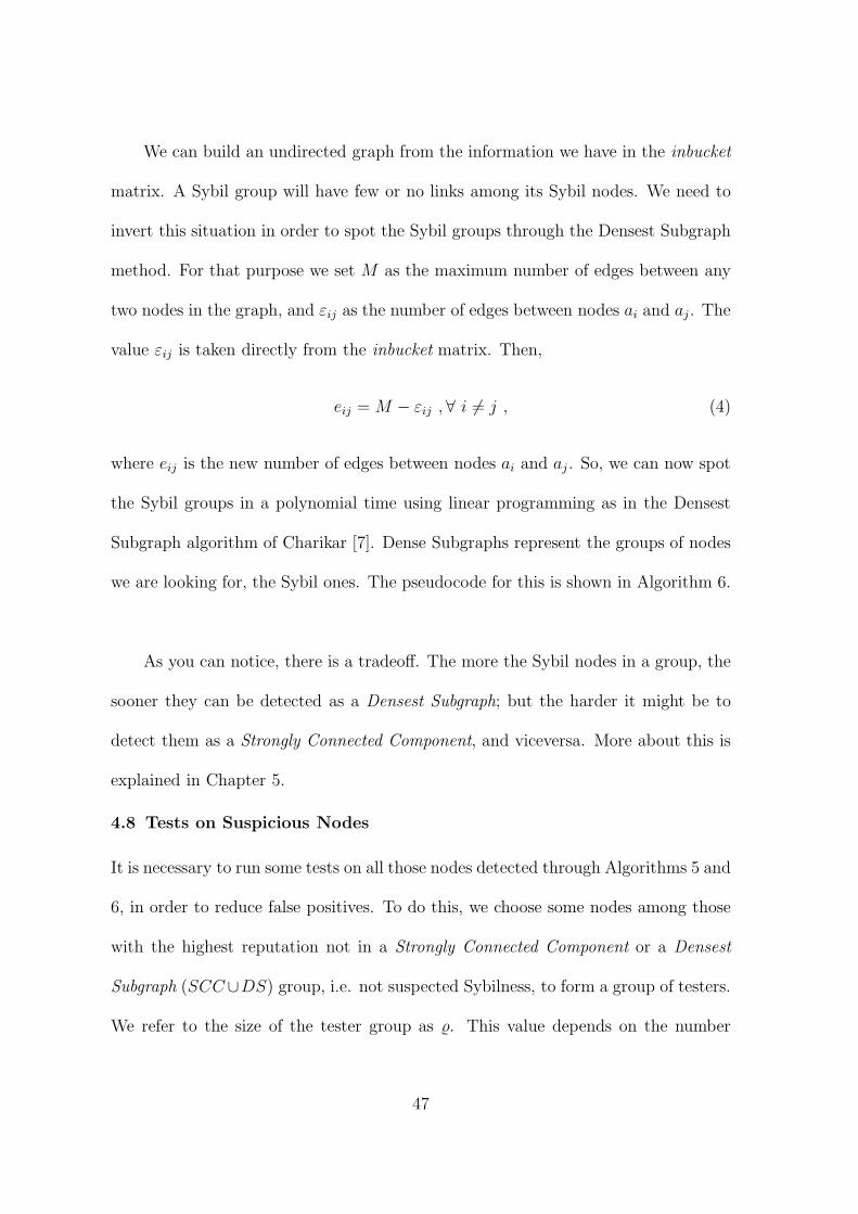
We can build an undirected graph from the information we have in the inbucket

matrix. A Sybil group will have few or no links among its Sybil nodes. We need to

invert this situation in order to spot the Sybil groups through the Densest Subgraph

method. For that purpose we set M as the maximum number of edges between any

two nodes in the graph, and εij as the number of edges between nodes ai and aj . The

value εij is taken directly from the inbucket matrix. Then,

eij = M − εij , ∀ i 6= j , (4)

where eij is the new number of edges between nodes ai and aj . So, we can now spot

the Sybil groups in a polynomial time using linear programming as in the Densest

Subgraph algorithm of Charikar [7]. Dense Subgraphs represent the groups of nodes

we are looking for, the Sybil ones. The pseudocode for this is shown in Algorithm 6.

As you can notice, there is a tradeoff. The more the Sybil nodes in a group, the

sooner they can be detected as a Densest Subgraph; but the harder it might be to

detect them as a Strongly Connected Component, and viceversa. More about this is

explained in Chapter 5.

4.8 Tests on Suspicious Nodes

It is necessary to run some tests on all those nodes detected through Algorithms 5 and

6, in order to reduce false positives. To do this, we choose some nodes among those

with the highest reputation not in a Strongly Connected Component or a Densest

Subgraph (SCC∪DS) group, i.e. not suspected Sybilness, to form a group of testers.

We refer to the size of the tester group as . This value depends on the number

47

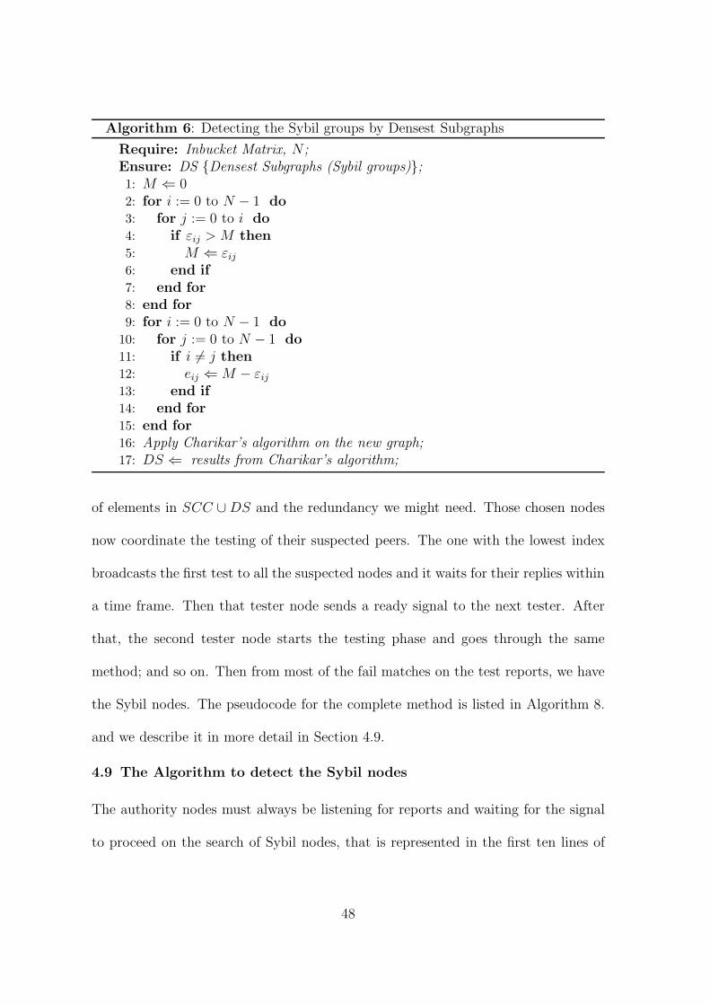
Algorithm 6: Detecting the Sybil groups by Densest Subgraphs

Require: Inbucket Matrix, N ;Ensure: DS Densest Subgraphs (Sybil groups);1: M ⇐ 02: for i := 0 to N − 1 do

3: for j := 0 to i do

4: if εij > M then

5: M ⇐ εij

6: end if

7: end for

8: end for

9: for i := 0 to N − 1 do

10: for j := 0 to N − 1 do

11: if i 6= j then

12: eij ⇐ M − εij

13: end if

14: end for

15: end for

16: Apply Charikar’s algorithm on the new graph;17: DS ⇐ results from Charikar’s algorithm;

of elements in SCC ∪ DS and the redundancy we might need. Those chosen nodes

now coordinate the testing of their suspected peers. The one with the lowest index

broadcasts the first test to all the suspected nodes and it waits for their replies within

a time frame. Then that tester node sends a ready signal to the next tester. After

that, the second tester node starts the testing phase and goes through the same

method; and so on. Then from most of the fail matches on the test reports, we have

the Sybil nodes. The pseudocode for the complete method is listed in Algorithm 8.

and we describe it in more detail in Section 4.9.

4.9 The Algorithm to detect the Sybil nodes

The authority nodes must always be listening for reports and waiting for the signal

to proceed on the search of Sybil nodes, that is represented in the first ten lines of

48

Algorithm 7: Testing the nodes to corroborate the Sybilness

Require: suspected nodes, reputation list by rank;Ensure: SN Sybil nodes;1: total suspected ⇐ total of suspected nodes2: testers,r ⇐ ⌈total suspected/10⌉3: a,b,i⇐04: while a < r do

5: while i < total suspected do

6: if reputation rank[a] == suspicious[i] then

7: r=r+18: break9: else

10: if i == total suspected-1 then

11: testers[b] = reputation rank[a]12: b=b+113: end if

14: end if

15: i=i+116: end while

17: a=a+118: end while

19: for i:=0 to testers do

20: if MyID == testers[i] then

21: testvector[from j:=0 to size]⇐ random numbers22: k ⇐10i+123: Broadcast testvector to suspiciousk , suspiciousk+1, . . ., suspiciousk+924: Wait for the sortedvector from the suspicious nodes25: Verify the promptness of the reply26: Report results27: Break28: else

29: if MyID == suspicious[i] then

30: k = ⌊i/10⌋31: Receive the testvector from testers[k]32: sortedvector ⇐ Apply Quicksort to testvector33: Send sortedvector to tester[k]34: Break35: end if

36: end if

37: end for

49

the pseudocode of Algorithm 8. Every time they receive reports, they fill out their

matrices through the Algorithms 1, 2 and 3. Once there is enough information in

the matrices, this is after several hundreds time buckets, any node can broadcast a

signal requesting to proceed on the search of Sybil nodes. Then the authority nodes

(all the nodes can be authority nodes at the same time) run the Algorithms 5 and 6

looking for Strongly Connected Components and Densest Subgraphs, then from the

total of suspected nodes found, we determine the total of tester nodes needed, which

is about 10% of the total of suspected nodes found plus two (line 14), adding two is

just for redundancy to avoid having only one tester in the cases of low number of

suspected nodes.

Then we can proceed with the selection of the tester nodes (from line 15 to

17), they are chosen among those nodes with higher reputation and not in group of

suspected. There is a minimum value of reputation required to be a tester node,

this value is γ and it is set from the median of reputation points. Once the tester

nodes are defined, they proceed with the testing of the suspected nodes (lines 18

to 27). The first tester broadcast the test to the suspected nodes and waits for the

replies. The suspected nodes must reply within a time range of at most 32τ where τ

is the mean or average time required for the reply.

Those nodes that reply out of the allowed range are marked by that tester node

and then it broadcast the results to all the tester nodes and sends a ready signal to

the next tester node, which execute the same commands, and so on for all the tester

50

nodes. A more detailed pseudocode about the testing is given in Algorithm 7 and it

has a variant, the tester nodes work simultaneously (in parallel) testing the suspected

nodes by blocks of one tenth. This is to speed up the testing process in case we have

a high number of suspected nodes. The last steps are for the sum of the results from

all the testers (lines 29 to 38), if a suspected node failed in three quarters of the tests

or more, then it is considered a Sybil node.

4.10 The Running Time

In our method explained here in chapter 4, we use the greedy approximation

algorithm of Charikar [7] for finding dense components in a graph. In the case of this

algorithm, it has a complexity of O(m + n log n), where m represents the number of

edges and n represents the number of vertices or nodes.

We also use the Tarjan’s algorithm [19], in this case to find the Strongly Con-

nected Components; The complexity for this other algorithm is O(m + n). So, it is

easy to see that the total running time for our algorithm described in this chapter is

bounded to O(m + n log n).

51

Algorithm 8: The complete process of detecting the Sybil nodes

Require: Reputation Matrix, Counter Matrix, Inbucket Matrix, N , γ, σ, τ ;Ensure: SN Sybil nodes;1: while true do

2: Listen for reports3: if reports received then

4: Call algorithms 1, 2 and 35: end if

6: Listen for Sybil search signal7: if Sybil search signal received then

8: Continue from line 119: end if

10: end while

11: Call algorithm 5 (Input:Reputation Matrix, Counter Matrix, N , σ;Returns: SCC;)

12: Call algorithm 6 (Input:Inbucket Matrix, N ; Returns: DS;)13: x ⇐ |SCC ∪ DS|14: z ⇐ ⌈ x

10⌉ + 2

15: for i := 0 to z − 1 do

16: Select testeri

Where: testeri /∈ SCC, DS and testeri reputation > γ ;17: end for

18: for i := 0 to z − 1 do

19: testeri broadcast the test to the SCC ∪ DS nodes;20: while time > 2τ do

21: testeri listen22: if nodexj

does not reply within 32τ then

23: Kixj⇐ 1

24: end if

25: end while

26: Broadcast of the results to all the testers27: Ready signal for testeri+1

28: end for

29: for j := 0 to x − 1 do

30: y ⇐ 031: for i := 0 to z − 1 do

32: y ⇐ y + Kixj

33: end for

34: if y > 34z then

35: nodexj∈ SN

36: end if

37: end for

38: Return SN

52

CHAPTER 5

SIMULATION RESULTS

A network environment was modeled with different percentages of Sybil nodes under

the control of malicious user. Those Sybil nodes pretend to interact among them in

order to build false reputations, claiming to be independent and trustworthy nodes,

which is the foundation for the Sybil attack. We show next the outcomes of the

simulations after thousands of experiments.

5.1 Detection by Strongly Connected Components

The point at coordinates (1800,50) of Figure 2 shows that in a network with 10% of

Sybil nodes and after one thousand eight hundred time buckets of information, in one

hundred experiments, fifty showed at least one or more of the honest nodes strongly

connected with another, without being part of the Strongly Connected Components.

Fig. 2. Detection results by the Strongly Connected Components method for every onehundred experiments with 5% and 10% of Sybil nodes respectively.

53

In the results of the experiments showed at Figures 2 and 4, at every time

bucket, there were always ten percent of the total of nodes (honests plus Sybils)

interacting and broadcasting. Those nodes were chosen randomly every time. In

Figures 2 and 4 we see that the less the percentage of Sybil nodes, the sooner

they can be detected as a Strongly Connected Component, this supposing that the

malicious user is using all his/her Sybil nodes to earn reputation points between

them, in order to make them appear trustworthy. This is because the more the

Sybil nodes, the less the reputation points needed from every Sybil peer to total

the minimum required to be considered trustworthy. In other words, the more

the Sybil nodes, the reputation points earned between them can be more diffused

and consequently their Sybil connections appear weaker. For that reason, different

values of σ (the threshold value described in Section 4.6) has to be tried to detect

the Sybil nodes as a Strongly Connected Component. There is a tradeoff here, if the

value of σ is too low, many honest nodes might appear “strongly connected” but not

necessarily forming a group; on the other hand if the value of σ is high, it is easier

for a malicious user to evade this detection, following is an illustrative example for

this case.

The Sybil nodes could be so many and their reputation points and interactions so

widely dispersed that they could avoid appearing as a Strongly Connected Component.

This is not an easy task, in a group of n Sybil nodes, it would take at least Ω(n)

operations for a Sybil node to simulate an interaction with every other Sybil peer

(see figure 3). So, it would take at least Ω(n2) operations in total for all the Sybil

54

Fig. 3. Sybil nodes simulating an interaction with their Sybil peer a, in order to boosttheir reputation points.

nodes to interact with all their Sybil peers. If every Sybil interaction is reported with

about the same amount of reputation points, then the affinity of one node with any

other node would be ≈ 2n

and this value just need to be under the lower threshold

(or value of σ described in Section 4.6) to avoid this specific detection method. All

that is nothing straightforward for a malicious user who needs big values of n and the

costly Ω(n2) interactions in order to give high reputation to all his/her Sybil nodes

without making them appear as a Strongly Connected Component.

Although, a malicious user can concentrate the effort in giving high reputation

to few or only to one of his/her Sybil nodes, in that case he/she would require only

Θ(n) interactions but still a big value of n. On the other hand, the more the Sybil

nodes created by a malicious user, the more those nodes will be exposed by the

other detection method (see Sections 4.7 and 5.2) and appear as a Densest Subgraph

by the timing of their broadcasts.

In Figure 5 are shown the results for the detection by the Strongly Connected

Component method for the cases of 5% and 10% of Sybil nodes in the network. The

point at coordinates (1000,18.53) means that for the case of a network with 10%

55

Fig. 4. Detection results through the Strongly Connected Components method for everyone hundred experiments with 15% and 20% of Sybil nodes respectively.

of Sybil nodes, after one thousand time buckets, there are in average 18.53 honest

nodes appearing strongly connected to others and not necessarily interconnected

forming a group, which is in most of the cases. Similar results are shown in

Figure 6, the difference is that the more the Sybil nodes the more the time buckets

of observation needed to find the proper relations. The results shown in Figures 5

and 6 corresponds to an activity, at every time bucket, of 10% of the total of the nodes.

The results shown in Figure 7 represent the outcome of the experiments

with an activity, at every time bucket, of 20% of the total of the nodes. Since

there is more participation, the relationships among the nodes can be detected sooner.

56

Fig. 5. Detection results by the Strongly Connected Components method in the cases of5% and 10% of Sybil nodes situation. The “x” axis represents the time buckets.

5.2 Detection by Densest Subgraphs

The Sybil nodes can also gain all their reputation points honestly and they will

not appear as a Strongly Connected Component, avoiding this way just one of our

detection methods. In this case our algorithm prevents the nodes from cheating on

the reputation points.

In Figure 8 are shown the results of some experiments. As can be seen, the fewer

the Sybil nodes, the more the time buckets (or information in the inbucket matrix)

that is needed to detect the Densest Subgraphs. In Figure 8, the point at coordinates

(1400,53) means that in one hundred experiments in a network with 10% of Sybil

nodes and using only one thousand and four hundred time buckets, fifty three of the

57

Fig. 6. Detection results by the Strongly Connected Components method in the cases of15% and 20% of Sybil nodes situation. The “x” axis represents the time buckets.

experiments had at least one honest node connected to another and not necessarily

as part of a Densest Subgraph. As more information is in the inbucket matrix, the

number of those honest nodes connected to others tend to be zero. For this method,

it is easier to detect a group of Sybil nodes in a network with a high percentage of

them. Since they are limited in their capacity of broadcasting together, the bigger

the group, the more they are exposed and fewer the time buckets required to spot

them.

The results shown in Figure 9 represent how many honest nodes are connected

with others. In Table 13 is shown a tiny example just as an illustration of this.

Supposing that the nodes labeled from zero to four are Sybil, they form a clique

58

Fig. 7. Detection results by the Strongly Connected Components method in the cases of10%, 15% and 20% of Sybil nodes situation. The “x” axis represents the time buckets.

that can be detected as a Densest Subgraph; while there are other connections, those

are loose, i.e. they do not form a group that would appear as a Densest Subgraph.

Returning to the Figure 9, the coordinates (1000,31.5) means that in an environment

with 5% of Sybil nodes, after one thousand of time buckets, there are in average 31.5

honest nodes that are connected with others.

59

Fig. 8. Detection results by the Densest Subgraph method in the presence of differentpercentages of Sybil nodes.

Fig. 9. Detection results by the Densest Subgraph method in the cases of 5%, 10%, 15%and 20% of Sybil nodes environment. The “x” axis represents the time buckets.

60

η0 → η1, η2, η3, η4.η1 → η0, η2, η3, η4.η2 → η0, η1, η3, η4.η3 → η0, η1, η2, η4.η4 → η0, η1, η2, η3.η8 → η52

η21 → η83

η27 → η78, η84.

TABLE 13. Example of connections among nodes.

61

CHAPTER 6

CONCLUDING REMARKS AND FUTURE WORK

Our algorithm works well in local area networks, but communication and timing

problems arise as the network size increases. The basic solution for this case would be

to divide big networks into smaller ones and create clusters of observers or distributed

authority groups that would interchange their information. However, new issues and

coordination problems appear when a node of one group interacts with a node of

another group. Either we can create a distributed authority group only for those

cases (if there are few of them), or just ignore those interactions. In this last case it

would be easier for a malicious user to hide his/her Sybil nodes among the different

groups, and to some extent, avoid detection by the Strongly Connected Components

and Densest Subgraph algorithms, as explained in Sections 4.6 and 4.7 respectively.

For that case this is still an open problem, as is the case of several colluding malicious

users that can operate several Sybil nodes simultaneously in order to make them

appear as trustworthy independent ones.

6.1 Conclusions

We showed a novel system to detect Sybil nodes and prevent Sybil attack. We

combine some ingredients from earlier work, but as far as we know, this is the first

approach that addresses both the static and the dynamic networks. We use here a

distributed authority to keep track of the nodes’ behavior and reputation, and detect

the Sybil nodes through Strongly Connected Components and/or Densest Subgraphs.

After that, tests are run on the suspected nodes in order to eliminate any false

positives. Our algorithm is effective even in the presence of a high percentage of

Sybil nodes in the system. The algorithm is easy to implement and requires not

62

high memory resources, the total running time for it is bounded to O(m + n log n)

as explained in 4.10.

63

REFERENCES

[1] J. Aspnes, C. Jackson, and A. Krishnamurthy. Exposing computationally-challenged Byzantine impostors. Technical Report YALEU/DCS/TR-1332, YaleUniversity Department of Computer Science, July 2005.

[2] R. A. Bazzi and G. Konjevod. On the establishment of distinct identities inoverlay networks. Distributed Computing, 19(4):267–287, 2007.

[3] C. Buragohain, D. Agrawal, and S. Suri. A game theoretic framework for incen-tives in p2p systems. In Peer-to-Peer Computing, 2003. (P2P 2003). Proceed-ings. Third International Conference on, pages 48–56, Sept. 2003.

[4] S. Capkun and J.-P. Hubaux. Secure positioning of wireless devices with appli-cations to sensor networks. In Proceedings of INFOCOM, 2005.

[5] S. Capkun and J. P. Hubaux. Secure positioning in wireless networks. IEEEJournal on Selected Areas in Communications, 24(2):221–232, 2006.

[6] J. Cardenas-Haro and G. Konjevod. Detecting sybil nodes in static and dy-namic networks. In R. Meersman, T. Dillon, and P. Herrero, editors, On theMove to Meaningful Internet Systems, OTM’10, volume 6427 of Lecture Notesin Computer Science, pages 894–917. Springer Berlin / Heidelberg, 2010.

[7] M. Charikar. Greedy approximation algorithms for finding dense components ina graph. In K. Jansen and S. Khuller, editors, APPROX, volume 1913 of LectureNotes in Computer Science, pages 84–95. Springer, 2000.

[8] R. M. Cooke. Experts in Uncertainty: Opinion and Subjective Probability inScience (Environmental Ethics and Science Policy). Oxford University Press,USA, October 1991.

[9] T. H. Cormen, C. Stein, R. L. Rivest, and C. E. Leiserson. Introduction toAlgorithms. McGraw-Hill Higher Education, 2nd edition, 2001.

[10] J. R. Douceur. The sybil attack. In IPTPS, pages 251–260, London, UK, 2002.Springer-Verlag.

[11] T. Gneiting and A. E. Raftery. Strictly proper scoring rules, prediction, andestimation. Technical report, Journal of the American Statistical Association,2004.

[12] C. Lesniewski-Laas. A sybil-proof one-hop dht. In SocialNets ’08: Proceedingsof the 1st Workshop on Social Network Systems, pages 19–24, New York, NY,USA, 2008. ACM.

[13] N. Miller, P. Resnick, and R. Zeckhauser. Eliciting informative feedback: Thepeer-prediction method. Manage. Sci., 51(9):1359–1373, 2005.

[14] J. Newsome, E. Shi, D. Song, and A. Perrig. The Sybil attack in sensor networks:analysis and defenses. In Proc. of IPSN, 2004.

64

[15] M. J. Osborne. An Introduction to Game Theory. Oxford University Press,USA, 2004.

[16] C. Piro, C. Shields, and B. N. Levine. Detecting the sybil attack in mobile adhoc networks. In Securecomm and Workshops, 2006, pages 1–11, 28 2006-Sept.1 2006.

[17] D. M. Ritchie and K. Thompson. The unix time-sharing system. Commun.ACM, 17(7):365–375, 1974.

[18] N. Sastry, U. Shankar, and D. Wagner. Secure verification of location claims. InProc. of ACM WiSe, 2003.

[19] R. E. Tarjan. Depth-first search and linear graph algorithms. SIAM J. Comput.,1(2):146–160, 1972.

[20] B. R. Waters and E. W. Felten. Secure, private proofs of location. TechnicalReport TR-667-03, Princeton, 2003.

[21] S. S. Wilks. Mathematical statistics. New York, Wiley, 1962.

[22] H. Yu, P. B. Gibbons, M. Kaminsky, and F. Xiao. Sybillimit: A near-optimalsocial network defense against sybil attacks. In IEEE Symposium on Securityand Privacy (Oakland’08), 2008.

[23] H. Yu, M. Kaminsky, P. B. Gibbons, and A. Flaxman. Sybilguard: defendingagainst sybil attacks via social networks. In SIGCOMM, pages 267–278, 2006.

65

detecting sybil nodes in static and dynamic networks by

Documents