detecting electromagnetic fields: the heterodyne principle ... · pdf filedetecting...

Introduction to Astrophysical Instrumentation: Radio Lab July 28 & 29, 2015

Detecting Electromagnetic Fields:

The Heterodyne Principle and Simple Antennas

Introduction to Astrophysical Instrumentation

Dunlap Institute, University of Toronto

Introduction:

Radio Astronomy is a relatively new field of science, having existed for less than 100 years. In 1864 (published in 1865), James Clerk Maxwell unified the theories of electricity and magnetism, and stated that light was, in fact, an example of an electromagnetic (EM) wave (also predicting the existence of other EM waves, including radio waves). A generation later, in 1888, Heinrich Hertz demonstrated the existence of radio waves with his tuned resonant spark-gap experiment, which in turn paved the way for wireless communication, as championed by Karl Braun, Guglielmo Marconi, and others in the late 1890s and early the next century. With antenna theory developing (Braun invented phased arrays of antennas to improve directionality and gain), and even continuous wave transmission and detection available in the early 1900s (Reginald Fessenden), why was it that astronomy overlooked this new window to the universe? Why did it take until 1932 for a Bell Labs radio engineer to notice signals from outer space, and then half a decade before anyone else pursued this?

In part, it was not that scientists overlooked the radio portion of the electromagnetic spectrum; they simply failed to find anything in their many initial attempts near the turn of the century, and then concluded, erroneously, that there should be nothing to observe. The early scientists made their mistake based on the theory that EM emissions from space should come from blackbody radiation of stars, and should thus be insignificant in the radio band. In the intervening years there were many new technologies developed and refined, so it was when Karl Jansky was tasked to determine the source of static plaguing wireless transmissions that extra-terrestrial sources of radio waves were discovered. This event was noted with some excitement when it was published in the New York Times on May 5, 1933, but the radio hiss from outside of our solar system was not a project that Bell Labs wished to pursue so Jansky moved on to other projects. His discovery also occurred during the Great Depression (1929-1939), so funding was low. Grote Reber, an electrical engineer and HAM radio operator, was inspired by the article about radio hiss from the centre of the galaxy, and applied to work with Jansky at Bell Labs, but was unsuccessful in his applications. Instead of being discouraged, he continued his job and simultaneously built a radio telescope with his own money and started to map out the universe in the radio portion of the EM spectrum, successfully detecting radio signals from the Milky Way in


1938. With Reber’s publications in astronomical journals starting in 1940, the field of radio astronomy grew quickly, and has often been at the leading edge of technology.

As well as synchrotron radiation and thermal sources, the 21 cm Hydrogen Line, caused by the transition of the proton and electron having parallel spins to anti-parallel spins, is of great importance to radio astronomers and cosmologists. Since hydrogen is the most common element in the universe, this radiation, at 1420.4 MHz, can be used as a proxy for matter, and by observing red shifted hydrogen, we can build up matter density maps throughout our cosmological history.

The goals for this laboratory session are to:

1) Understand the basic circuit chain in translating a wave in the sky to a wave in a waveguide (i.e. an electrical signal we can measure)

2) Understand the heterodyne principle, which is key for detecting signals

3) Use waterfall plots to show sensitivity at different wavelengths

4) Create (draw with conductive ink) a working, tuned dipole antenna for radiation at 1420 MHz

a. Relate geometric shape to resonant wavelengths being detected

b. See the effects of line width on resonance lengths

5) Understand how gain and directivity are related; see how important anechoic chambers are for accurate testing

6) See a variety of antenna designs and combination patterns and understand how they are useful in different contexts

7) Observe the sky


Lab Equipment:

1 AirSpy Device

Laptop with the program ‘gqrx’ installed (on Linux)

CircuitScribe Conductive Ink Pen

White eraser

1 Edge-mount SMA connector

1 fiberglass (FR4) board modified with a circular mount point on one side

Glossy Photo Printing Paper

Tape to mount the paper to FR4

1 rotating tray (AKA ‘Lazy Suzan’) with tube antenna stand attached

360o Protractor (Paper printout)

Acrylic Ruler

Multimeter with probes

1 coaxial cable with SMA connectors


The AirSpy:

In this lab we will be using the commercially available AirSpy Device, which has a tunable frequency range of 24-1800 MHz via a heterodyne mixer. Figure 1 is a photo of the inside of the device, with all of the I/O connectors labeled (though we will only use the antenna plug and micro USB today). In figure 2, you can see the related basic circuit diagram. As well as having a tunable Local Oscillator (LO), a nonlinear mixer, and an Intermediate Frequency filter, the Raphael tuner chip has three gain adjustments. There is the Low Noise Amplifer (LNA) which increases the strength of the input signal, the mixer amplifier to boost the signal after the two signals are mixed, and the Intermediate Frequency (IF) amplifier, which boosts the resulting signal after it has been filtered for a desired frequency band.

!

Figure 1) A photo of the inside of the AirSpy. This device is capable of tuning frequencies from 24-1800 MHz and, at its simplest, all you need is an antenna for the input and a computer to output the sampled data. However, you can do much more with it as evidenced by the inclusion of an external clock input, General Purpose Input/Output ports, and a Joint Test Action Group (JTAG) serial port. Code bases are open-source.


!

Figure 2) A block diagram of the circuit. The Rafael tuner (small black square in approximately the middle of Fig. 1) contains the Low Noise Amplifier (LNA), the Local Oscillator (LO), the heterodyning mixer, the mixer amplifier, the Intermediate Frequency (IF) filter, and the IF amplifier. The LPC4370 SOC (large chip in Fig. 1) does the analog to digital conversion (ADC) and transmits the data to the computer over the USB port.

JavaScript Heterodyning Program (15 min)

Goals: work through the math demonstrated in the lecture, showing that trigonometric identities can explain what the new frequencies will be, and play with a JavaScript demo to see how the spectra are affected.

In radio signal processing, the technique to mix two signals together at a new frequency was invented by Reginald Fessenden in 1901 and is called ‘heterodyning’ signals. The word ‘Heterodyne’ has Greek roots and refers to different powers rather than different frequencies (hetero: other, dunamis!dyne: power), but this may have just been referring to the fact that the carrier and signal were of differing powers.

This concept is very important for both instrumental radio telescopes and information transmission/reception, since it allows us to shift the frequency of a signal to one that is more convenient. For data transmission, this means that many signals can be transmitted in a given frequency band without interfering (while at the same time keeping receivers relatively simple). For data reception, it can simplify circuit designs and/or allow one to sample data that would otherwise be at an inaccessible frequency band.

As you saw in the lectures, a heterodyning circuit is comprised of an amplifier, an input signal, a local-oscillator (LO), a non-linear mixing unit, and a filter. Initially, the local oscillator was kept at a constant frequency, and filters were made tuneable. This, however, is quite difficult for high quality filtering, so now it is the local oscillator that is varied and the filter remains constant.

Local Oscillator(LO) Synthesizer

Intermediate Frequency (IF) Filter

Antenna Low NoiseAmplifier

(LNA) MixerTo ADC

and Computer

MixerGain

IF Gain


In this first section, before using the AirSpy with the software defined radio (SDR) system to receive electromagnetic waves, you will use an interactive Javascript program to play with the concepts described in the lecture. You will see the effects of varying the LO frequency on the power spectra and, for fun, will see how signals can be transmitted in a frequency band centred at a different carrier frequency.

The result of a linear mixer will be a signal that is comprised of the weighted sum of the two input signals, while the resulting signal from a nonlinear mixer will include higher order powers of their sum. The math behind a nonlinear mixer is quite straightforward, but to understand heterodyne mixers, it helps to work through it at least once.

Let S1 = a sin(2πf1t) And S2 = b sin(2πf2t)

where a, b, are scaling factors, f1, and f2 are frequencies, and t represents time. The output of a non-linear mixer will be

Vout = α1(S1+S2) + α2(S1+S2)2 + higher order terms of decreasing amplitude…

Vout = α1(S1+S2) + α2(S12 +2S1S2 +S22) + …

where α1, and α2 are also scaling factors. The term that makes the heterodyne mixer work is α2(2S1S2). The extra terms will be present in the signal, but filters take can be used to remove their effects, most of the time.

Using trigonometric identities, or Euler’s formula, show that

S1 S2 = ½ ab[cos(2π|f1-f2|t) – cos(2π(f1+f2)t)]

which explains how the resulting signal has shifted frequency bands. What other frequencies would you expect there to be peaks at (in an unfiltered post-heterodyne mixer signal)?


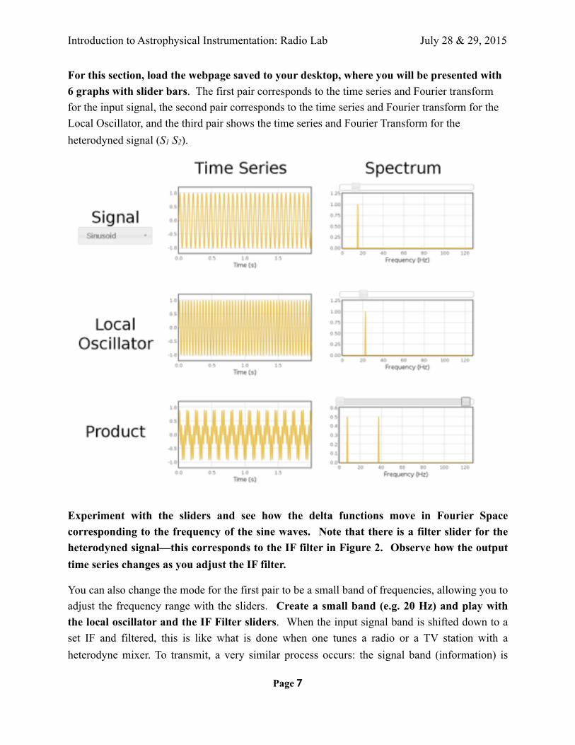
For this section, load the webpage saved to your desktop, where you will be presented with 6 graphs with slider bars. The first pair corresponds to the time series and Fourier transform for the input signal, the second pair corresponds to the time series and Fourier transform for the Local Oscillator, and the third pair shows the time series and Fourier Transform for the heterodyned signal (S1 S2).

!

Experiment with the sliders and see how the delta functions move in Fourier Space corresponding to the frequency of the sine waves. Note that there is a filter slider for the heterodyned signal—this corresponds to the IF filter in Figure 2. Observe how the output time series changes as you adjust the IF filter.

You can also change the mode for the first pair to be a small band of frequencies, allowing you to adjust the frequency range with the sliders. Create a small band (e.g. 20 Hz) and play with the local oscillator and the IF Filter sliders. When the input signal band is shifted down to a set IF and filtered, this is like what is done when one tunes a radio or a TV station with a heterodyne mixer. To transmit, a very similar process occurs: the signal band (information) is


mixed with a higher second frequency, one of the two resulting bands is either mixed out or filtered out, then the resulting shifted signal is transmitted over the air.

Additional Information: on Fourier transforms and aliasing

Note that some puzzling behaviours that can be observed when adjusting the sliders… For instance, the amplitude of the sine waves are constant, but when the frequency is set too high compared to the sampling rate, the resulting sinusoid will not be plotted correctly; it will appear to vary in amplitude.

Fourier transforms are based on sinusoids, so there are repetitions that can occur when frequencies should lie outside of the frequency band you are interested in. This is called aliasing. When a portion of the frequency band goes out of range, it may wrap around and come back into the current frequency band.


Familiarization with the Software Defined Radio (SDR) program, ‘gqrx’ and Tuning into a local FM Radio Station (15 min):

Goals: get the AirSpy unit working with a whole line of components, but with no ‘real’ antenna yet. Learn what the settings names are and mean, change the various amplification settings, and continue with concepts about heterodyning signals without worrying about the antenna itself, by tuning into a local radio station.

Open the SDR program, ‘gqrx’ and, with the procedure below, try to find and tune in local radio stations. While you don’t have a properly tuned antenna built yet, the leads on the SMA connector will act as a very poor gain omni-directional antenna because the lead lengths are much shorter than half a wavelength. Because we are so close to the CN tower, which acts as a transmitter for many stations, the fact that they are terrible antennas should not matter. You’ll be building a real antenna soon, tuned for a specific frequency.

Basic AirSpy Setup: Attach the edge-mount SMA connector to one end of the 50 Ohm Coaxial cable and the other end to the SMA connector to the AirSpy unit. Connect the AirSpy to the computer via the USB cable and start up the ‘gqrx’ program in a terminal window (the terminal program can be found under ‘favourites’ in the main desktop menu).

Computer_Name $ > gqrx <enter>

a) If a settings menu appears then first select the AirSpy device and then make sure the sampling frequency is set to 2500000 (if the AirSpy isn’t listed, select Other… and type ‘airspy’ in the device string line and type in the sampling frequency, manually).


! !

b) Click OK, then maximize the software defined radio

!


!


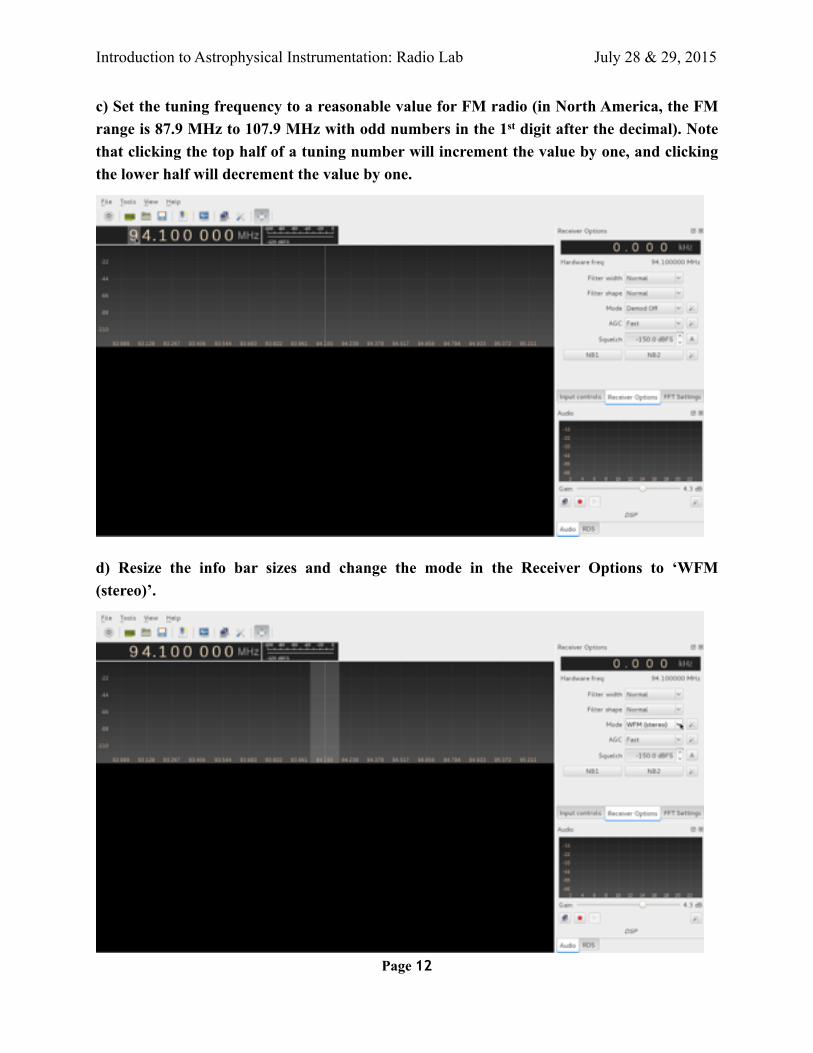
c) Set the tuning frequency to a reasonable value for FM radio (in North America, the FM range is 87.9 MHz to 107.9 MHz with odd numbers in the 1st digit after the decimal). Note that clicking the top half of a tuning number will increment the value by one, and clicking the lower half will decrement the value by one.

!

d) Resize the info bar sizes and change the mode in the Receiver Options to ‘WFM (stereo)’.

!


e) Turn the unit on for data sampling by pressing the ‘On’ button.

!

f) Click on the Input controls tab and adjust the gain settings (LNA should be the first thing to turn up). The end goal is a base noise floor of about -90 dB when no antenna is attached. For reference these are the amplifiers that were shown in Figure 2.

!


!

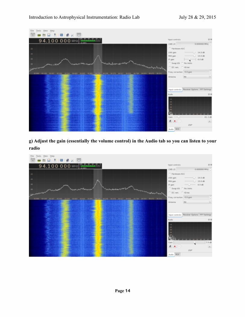
g) Adjust the gain (essentially the volume control) in the Audio tab so you can listen to your radio

!


h) Experiment with settings, noting that you can click on frequencies other than the central one.

!

i) Explore the FFT Settings tab, noting that mouse-over hovers give tool-tips.

!

j) Set your central frequency to 1420 MHz, and power down gqrx temporarily as you get ready to create an antenna tuned for this frequency.


The CircuitScribe: Conductive Ink Testing (10-20 min):

Goals: learn how to use the conductive ink pen, and characterize the resistances based on line width

The Circuit Scribe pen writes with a non-toxic, odour-free solution containing silver. The conductivity is dependent on the material written on, with glossy photo-printing paper for ink-jet printers yielding the lowest resistances. According to the manufacturer’s webpage (www.electroninks.com), the resistances are typically 2-10 Ohms per cm of writing when writing with fine lines. For an antenna, we would like to have very low electrical resistances per cm length, especially since our antennas will have arms on the order of 5 cm or more. To reduce the resistance per length, we can increase the width of our electrical traces and/or deposit more conductive ink in the same place.

On a piece of glossy photo paper, experiment with drawing techniques (parallel lines, tiny circles, drawing over the same area, etc.) and draw 2 cm long lines of varying widths (while staying less than ~0.5 cm thick). Note that if you draw too hard, you may tear into the paper making it difficult to erase.

What are the resistances for each technique? Does the ink dry quickly? Does the resistance change based on how fresh the ink is? Which drawing technique gives the most consistent and lowest resistance? How wide does a trace need to be for the resistance to approach the resistance of your leads on the multimeter?

http://www.electroninks.com


The Dipole Antenna: Drawing and building a tuned half-wavelength antenna (30 min)

Goals: Draw a dipole antenna and tune it to maximize the amplitude of the received signal.

A dipole antenna is one of the simplest frequency-tuned antenna designs. To understand how it works, a thought experiment can be done based on the transmission of signals at a specific frequency, since good transmitters are also good receivers at the same frequency (see Figure 3).

!

Adapted from https://commons.wikimedia.org/wiki/File:Dipole_antenna_standing_waves_animation_461x217x150ms.gif

Figure 3) If an alternating current generator is attached to two wires that are bent apart from each other, then when the total length is an odd integer multiple of ½ λ (1, 3, 5, etc.,), current nodes will occur at the tips of the wires (i.e. not much charge will move at the tips) and standing waves can occur. Overall, however, in part a) there will be a net accumulation of negative charge (surplus of electrons) at the left and a net positive charge (deficit of charge) at the right (using standard old-fashioned electrical conventions where positive charges are what move). This creates an electric field pointing to the left. One half-cycle later (part b) the situation is reversed and the electric field points to the right. If the dipole is centre-fed and is not an odd multiple of ½ λ, then standing waves will not occur and the situation will be less defined. Since good transmitters are also good receivers, when the generator is replaced by a receiver, the dipole will be most effective for alternating electric fields with wavelength ~ ½ λ. Thus, a centre-fed dipole will be best tuned for polarized electromagnetic waves with the dipole arms aligned with the electric field when the dipole length is an odd integer multiple of ½ λ. (One can design non-centre fed dipoles (i.e. arms of different length) that will work at non-odd-integer multiples of ½ λ, but those designs will not be covered here).

Dipole Creation Procedure:


1) Note the separation of the three prongs in a line on the edge-mount SMA board connector. The edge-mount connector has a very tight fit when put on the fiberglass (FR4) board with the glossy photo paper, so initial traces must be drawn on the paper before attaching the connector to the board and paper. Draw two leads starting from the edge of the paper and perpendicular to the paper edge that match the spacing of the centre pin and one of the side pins. Make sure they are long enough to clear the groove in the mounting tube when the board is mounted on the tube.

2) After giving your traces a short period of time to dry and checking their resistance with the multimeter (they should be close to the resistance of the leads—deposit more conductive ink if they are not), hold the edge-mount SMA adapter to your traces on the paper, and then, by pushing the paper + adapter group at a slight angle with respect to the FR4 board, wedge the SMA adapter and paper onto the board.

3) Measure the resistance between the pins and the leads—make sure they have good connections (very low resistances). If it is close to the same resistance as when you touch the leads together, then secure your sheet of paper to the board with tape.

4) Mount your FR4 board onto the support tube on the rotating tray (‘lazy Susan’) either in the vertical slot or by using the attachment on the back of the board.

5) Draw an antenna, lengthening each arm incrementally and keeping the position and orientation of the antenna with respect to the transmitter in the room constant. Remember to step away from the antenna while observing the signal amplitude in the power spectra/waterfall plot (people will interact with the EM waves in sometimes non-intuitive ways, as anyone with a TV antenna inside the place that they live will attest to).

6) Compare the length of your dipole tuned to maximize the reception of the generated signal with the theoretical length.

Note: The trace that you have drawn is not quite symmetrical... Since we have traces that are wider on the paper than they are thick, they will not quite have the same resonance based on the orientation of the paper (see Figure 4). Try mounting the antenna in its second mounting orientation and compare (qualitatively) the power of the signal. Also, draw a second antenna with wider traces and qualitatively note how the width affects the length needed to tune. Is there a significant difference, or is it virtually unchanged with our level of sensitivity here?


! Image from www.antenna-theory.com/antennas/broaddipole.php

Figure 4) Effect of wire width on resonant frequency for a 1.5 m half-wavelength dipole (i.e. λ = 3 m, so it is tuned for 100 MHz). When the wire diameter is 1/3000 the wavelength, the resonant frequency is roughly 96 MHz. When the diameter is 1/200 the wavelength, the resonant frequency drops again, but the bandwidth increases. By the time the diameter is 1/60 the wavelength the resonant frequency has shifted more than 10% the desired frequency. In general, increasing the trace thickness that you draw (usually wire diameter when people build their own antennas) will effectively lengthen the dipole, but will also broaden the band that can be received too.


Characterizing the antenna beam shape (30-60 min)

Goals: with the drawn antennas, rotate the antenna incrementally and note how the gain changes. Try to draw a rough beam pattern from this. Think about symmetry of the physical device and see if it is related to the shape of beam pattern in 3d.

Procedure: With the antenna mounted in the notches on the tube and the protractor below the glass turntable, orient your antenna so that the drawn antenna faces the transmitter. Lift the glass turntable (do not lift by the plastic tube) and rotate the protractor so that the 0° mark points toward the transmitter.

Next rotate the antenna 360° and see if there is any variation in the power (hopefully there is—if not, call one of the lab instructors to try to troubleshoot your setup).

Measured Power in dB = 10 log10, so 3 dB is a doubling in power. The waterfall plot will show the power as a colour variation, and the plot above it will allow you to estimate the peak power—it gives values in Power (dBFS), so it’s reference is the maximum voltage (Full Scale, or FS) that the AirSpy can handle. Common units in astrophysics and antenna theory include dBm (reference = 1 mW), dBW (reference = 1 W), and dBi (reference = isotropic antenna gain).

At the top of the screen, there is a green bar with a power level in dBFS that should correspond with the peak power shown on the power spectrum. If they agree, you can use that to help measure the power at various angles. (Make sure your tuned frequency line matches up with the peak).

Why is the second mounting orientation (i.e. using the ring on the back of the FR4 board to connect to the tube) non-ideal for this section? What is its axis of rotation?


Measure the power at multiple angles (no finer than 10°):

Sketch your pattern on the provided charts for the vertical and horizontal planes (spares are included). The concentric rings indicate power magnitude for a given angle. Make the largest ring your maximum power, and set the scale for the concentric rings appropriately. If you are so inclined, try to sketch a 3D gain map in the space below.

Angle (°) Power (db) Angle (°) Power (db) Angle (°) Power (db)

0 120 -120

10 130 -110

20 140 -100

30 150 -90

40 160 -80

50 170 -70

60 ±180 -60

70 -170 -50

80 -160 -40

90 -150 -30

100 -140 -20

110 -130 -10


Rotation around SMA feed point Rotation around drawn antenna


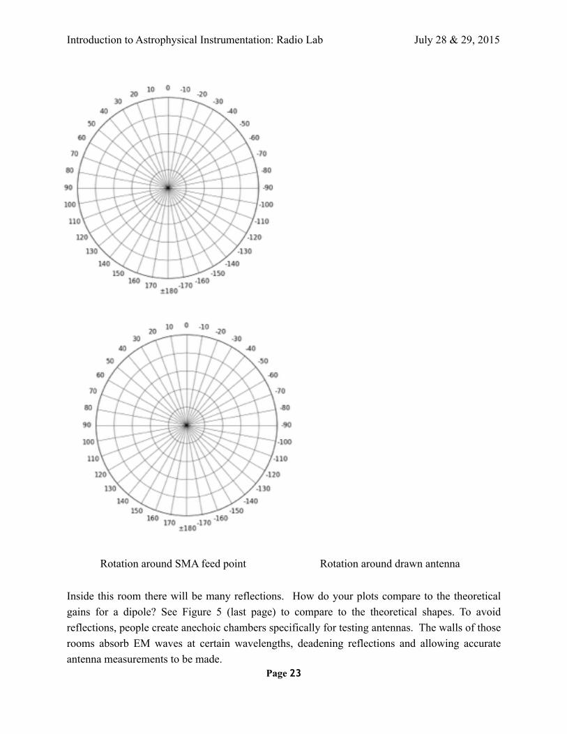
Rotation around SMA feed point Rotation around drawn antenna

Inside this room there will be many reflections. How do your plots compare to the theoretical gains for a dipole? See Figure 5 (last page) to compare to the theoretical shapes. To avoid reflections, people create anechoic chambers specifically for testing antennas. The walls of those rooms absorb EM waves at certain wavelengths, deadening reflections and allowing accurate antenna measurements to be made.


Investigating alternate shapes and their effects on bandwidth and gain/directivity (30 min)

Goals: Create a Yagi-Uda 2 element design (no electrical connection point), combine two dipole antennas in two of the three possible configurations: vertically stacked (broadside), and one dipole in front of the other pointed toward the source (end-fire or echelon). Think about how combining multiple dipoles in these different configurations may (qualitatively) affect the beam shape and gain based on interference arguments.

Yagi-Uda

The Yagi-Uda antenna uses conductive elements to condition the wave in free space near the antenna to increase the antenna gain (these conductors, are called ‘parasitic’ elements). It consists of a dipole antenna and 1 or more electrical conductors near the antenna which modify the incoming electromagnetic wave, essentially focusing the waves to the dipole. There are two 2 element variations for the Yagi-Uda design: One with a reflector behind the dipole, and one with a ‘steering element’ or ‘director’ in front of the dipole. The reflector should be at least 5% longer than the dipole to minimize end effects, and should be 0.15 to 0.25 λ behind it. Why should a reflector 0.25 λ behind the dipole help?

The ‘director’ should be 5% shorter than the dipole and 0.1 to 0.15 λ in front of it (http://www.ph.surrey.ac.uk/satellites/main/assets/schoolzone/project1/reflectors_directors.htm). The re-radiated wave will add with the wave naturally impinging on the antenna, increasing the gain in the forward direction.

$


Stacked and End-Fire Arrays

Stacked and end-fire arrays are essentially the same configuration in different orientations, but with different spacing between the electrically joined identical dipole elements. When the elements are vertically stacked, they should be separated by ½ λ for interference to cancel out signals above and below the array, and when they are one in-front of the other (end-fire) they should be separated by integer multiples of λ.

Build at least one of these two antenna arrays and try to see if they work as expected (is gain increased in the forward direction and decrease above and below the array?). Should there be a slight decrease in separation to account for the propagation speed in the conductor?

Observations of the sky with antennas at 21 cm (15-30 min)

Goals: Go outside and find the sun!

With stars acting as black-body radiation astronomers did not believe there would be much to see astronomically, so didn’t actually look for anything after initial tests were not conclusive. It was a radio engineer for Bell Laboratories, Karl Jansky, not an astronomer, who, while working to determine why there was interference in telephone calls, discovered radio sources from the centre of our galaxy in 1933 and accidentally started the field of radio astronomy and cosmology. The radio band is one of two windows for electromagnetic radiation, and the larger of the two (the other being the visible light band), but technology and bad luck had held up people from observing the sky until less than 100 years ago. Observe the sky with your new antenna (or antenna array) and see if you can observe any variations in the intensity as you point your antenna in different directions.

Additional Reading, for the curious:

Constantine A. Balanis, Antenna Theory: Analysis and Design, Wiley-Interscience, 2005.

General Reference: The ARRL Antenna Book by the American Radio Relay League (many editions; mine is the 17th edition (a practical guide for building antennas))

www.antenna-theory.com for basics of antennas: a great resource when beginning


National Radio Astronomy Observatory (NRAO): these websites cover both the history and theory for radio astronomy: searching www.nrao.edu will yield a lot of great information, and even a few online courses.

A.R. Thompson, J.M. Moran, and G.W. Swenson Jr, Interferometry and Synthesis in Radio Astronomy, Wiley-VCH, 2004. Not in the scope of this laboratory session, but a good reference if you are interested in the field.

Additional Resources:

!

Figure 5) Two views of the theoretical gain patterns for a ½ λ dipole antenna. Note that the gains are plotted logarithmically for this figure, to show a larger range of values. In your plot, you have a linear scale for the logarithms of the gains.

Additional Polar Plotting Paper:

http://www.nrao.edu

detecting electromagnetic fields: the heterodyne principle ... · pdf filedetecting...

Documents