detectability and state estimation for linear age

HAL Id: hal-01140166https://hal.inria.fr/hal-01140166v4

Submitted on 21 Oct 2016

HAL is a multi-disciplinary open accessarchive for the deposit and dissemination of sci-entific research documents, whether they are pub-lished or not. The documents may come fromteaching and research institutions in France orabroad, or from public or private research centers.

L’archive ouverte pluridisciplinaire HAL, estdestinée au dépôt et à la diffusion de documentsscientifiques de niveau recherche, publiés ou non,émanant des établissements d’enseignement et derecherche français ou étrangers, des laboratoirespublics ou privés.

Detectability and state estimation for linearage-structured population diffusion models

Karim Ramdani, Marius Tucsnak, Julie Valein

To cite this version:Karim Ramdani, Marius Tucsnak, Julie Valein. Detectability and state estimation for linear age-structured population diffusion models. ESAIM: Mathematical Modelling and Numerical Analysis,EDP Sciences, 2016, 50 (6), pp.1731-1761. �10.1051/m2an/2016002�. �hal-01140166v4�

https://hal.inria.fr/hal-01140166v4

https://hal.archives-ouvertes.fr

ESAIM: M2AN 50 (2016) 1731–1761 ESAIM: Mathematical Modelling and Numerical AnalysisDOI: 10.1051/m2an/2016002 www.esaim-m2an.org

DETECTABILITY AND STATE ESTIMATION FOR LINEARAGE-STRUCTURED POPULATION DIFFUSION MODELS

Karim Ramdani1, Marius Tucsnak

2and Julie Valein

2

Abstract. We investigate a state estimation problem for an infinite dimensional system appearing inpopulation dynamics. More precisely, given a linear model for age-structured populations with spatialdiffusion, we assume the initial distribution to be unknown and that we have at our disposal anobservation locally distributed in both age and space. Using Luenberger observers, we solve the inverseproblem of recovering asymptotically in time the distribution of population. The observer is designedusing a finite dimensional stabilizing output injection operator, yielding an effective reconstructionmethod. Numerical experiments are provided showing the feasibility of the proposed reconstructionmethod.

Mathematics Subject Classification. 92D25, 35R30, 93D15, 93B55.

Received April 13, 2015. Revised January 4, 2016. Accepted January 6, 2016.

1. Introduction and problem setting

We consider a linear age-structured population model with spatial diffusion described by the following system:⎧⎪⎪⎪⎪⎪⎪⎪⎪⎪⎪⎪⎨⎪⎪⎪⎪⎪⎪⎪⎪⎪⎪⎪⎩

∂tp(a, x, t) + ∂ap(a, x, t), a ∈ (0, a∗), x ∈ Ω, t > 0,

= −μ(a)p(a, x, t) + kΔp(a, x, t),

p(a, x, t) = 0, a ∈ (0, a∗), x ∈ ∂Ω, t > 0,

p(a, x, 0) = p0(a, x), a ∈ (0, a∗), x ∈ Ω,

p(0, x, t) =∫ a∗

0

β(a)p(a, x, t) da, x ∈ Ω, t > 0.

(1.1)

In the above equations:

• Ω ⊂ Rn, n � 1, denotes a smooth bounded domain, k is a positive constant diffusion coefficient and Δ thelaplacian with respect to the space variable x.

• p(a, x, t) denotes the distribution density of the population of age a at spatial position x ∈ Ω at time t;

Keywords and phrases. Inverse problems, observers, stabilization, population dynamics, spatial diffusion.

1 Inria, 54600 Villers-les-Nancy, France. [email protected] Universite de Lorraine, Institut Elie Cartan de Lorraine, UMR 7502, 54506 Vandœuvre-les-Nancy, France.

Article published by EDP Sciences c© EDP Sciences, SMAI 2016

http://dx.doi.org/10.1051/m2an/2016002

http://www.esaim-m2an.org

http://www.edpsciences.org

1732 K. RAMDANI ET AL.

O ⊂ Ω

0

a1

a2

a∗

y(t) := p|(a1,a2)×O

t = 0

t = T

Figure 1. How to estimate p(T ) as T → +∞ from the knowledge of y(t) for t ∈ (0, T )?

• p0 denotes the initial distribution;• a∗ ∈ (0,+∞) is the maximal life expectancy;• β(a) and μ(a) are positive functions denoting respectively the birth and death rates, which are supposed to

be independent of x (see Fig. 5 for typical graphs of these functions).

The last equation in (1.1) describing the birth process is the so-called renewal equation. We assume herehomogeneous Dirichlet boundary conditions (in space) which model a hostile habitat at the boundary ∂Ω,but other type of boundary conditions (in space) can also be considered (typically Neumann homogeneousboundary conditions which correspond to isolated population, i.e. vanishing incoming and outgoing flux).

In this paper, we investigate the following inverse problem (see Fig. 1):Assuming the initial age distribution p0 to be unknown, but knowing the age distribution

y(a, x, t) := p(a, x, t), t ∈ (0, T ), a ∈ (a1, a2), x ∈ O,

where O is some given subset of Ω and 0 � a1 < a2 � a, is it possible, and if so how, to estimate when T → +∞the age distribution p(a, x, T ), for x ∈ Ω and a ∈ (0, a∗)?

We provide a positive answer to this question and we propose an effective reconstruction algorithm. Basedon a semigroup formulation, our method crucially uses two main ingredients: the Luenberger observers [44] andthe fact that the problem has finitely many unstable eigenvalues (i.e. eigenvalues λ such that Re λ � 0). Let usmake this statement more precise by outlining in a formal way the main ideas of our reconstruction method.

Using a semigroup formulation, we first rewrite problem (1.1) in the abstract form (throughout the paper,the dot denotes the derivative with respect to time){

p(t) = Ap(t), t ∈ (0, T ),p(0) = p0,

where A : D(A) → X is the generator of a C0-semigroup on a Hilbert space X . Similarly, the availableobservation can also be reformulated using a bounded observation operator C ∈ L(X,Y ), where Y is anotherHilbert space:

y(t) = Cp(t), t ∈ (0, T ).

DETECTABILITY AND STATE ESTIMATION FOR LINEAR AGE-STRUCTURED POPULATION DIFFUSION MODELS 1733

We define the Luenberger type observer as the solution p of the following system

{˙p(t) = Ap(t) + L (Cp(t) − y(t)) , t ∈ (0, T ),p(0) = 0,

(1.2)

where L ∈ L(Y,X) is a linear operator to be chosen in such way that A+LC generates an exponentially stablesemigroup on X . Indeed, since the error e := p− p satisfies by construction

e(t) = (A+ LC)e(t), t ∈ (0, T ),

this condition ensures that e(T ) converges exponentially to 0, i.e. that (‖ · ‖ denotes the norm on X)

‖p(T ) − p(T )‖ � Me−ωT ‖p0‖,

showing that p(T ) constitutes an approximation of p(T ) as T → +∞. Let us emphasize that p(T ) can becomputed (by solving (1.2)) exclusively from the knowledge of the observation y(t), provided we have determineda stabilizing output injection operator L.

To compute this operator, we use the second main ingredient of our method: the fact that A has finitelymany unstable eigenvalues. Following Triggiani [63,64], we will show that the operator L can be easily deducedfrom the finite dimensional operator L+ stabilizing the finite dimensional system (A+, C+), where A+ is therestriction of A to the subspace X+ of X spanned by the unstable (generalized) eigenfunctions of A and C+ isthe corresponding observation operator.

For an overview on population dynamics models, we refer the reader to the monograph of Webb [67] andto the introductory paper [68]. Gurtin [27] introduced the first model with spatial diffusion (see also Gurtinand MacCamy [28]). For linear models, existence of a semigroup in L2 and large time asymptotics have beendeveloped by Chan and Guo in the case of homogeneous Dirichlet boundary (in [13] for age dependent birthand death rates and in [26] for age and space dependent birth and death rates) and by Huyer [33, 34] in thecase of homogeneous Neumann boundary conditions using perturbation techniques. The L1 setting has beeninvestigated by Rhandi [56] for a linear age-dependent model with spatial diffusion involving age and spacedependent birth and death rates. More recently, Walker [66] proposed an abstract functional analytic frameworkto study the large time behavior for an age-structured linear diffusive model. Existence and large time behaviorfor non linear models have been studied by Langlais [41, 42]. Exact and approximate controllability issues forage-structured dynamic systems have been studied in Ainseba and Langlais [3], Ainseba and Iannelli [1, 2],Traore [60], Traore and Kavian [37].

The literature on inverse problems for population dynamics models is less rich, especially when spatial diffu-sion is assumed. Without spatial diffusion, Pilant and Rundel [51], Rundell [57], Engl, Rundell and Scherzer [23]studied the determination of the death rate, Gyllenberg, Osipov and Paivarinta [29] investigated uniquenessfor the reconstruction of birth and death rates. State estimation problems, like the one considered here, havebeen considered only recently. Di Blasio and Lorenzi [21, 22] studied the well-posedness of the inverse problemof reconstructing the initial state for a linear age-dependent model. Traore investigated estimation problemsfor population dynamics, in which the state has to be recovered from distributed observation [62] or boundaryobservation [61] in space and full observation in age. However, he followed a non standard data assimilationmethod introduced by Puel [52,53] which is completely different from ours. In this approach, one computes thefinal state (or more precisely its coordinates in a suitably chosen Hilbert basis) by combining a zero controllabil-ity and optimal control results. To conclude, let us also mention the work of Perasso [49] in which identifiabilityissues are considered for an epidemiological model.


Unless otherwise stated, we will make the following classical assumptions on β and μ (see, for in-stance, [13, 20, 25]):• (Hβ) β ∈ L∞(0, a∗), β � 0 a.e. in (0, a∗);• (Hμ) μ ∈ L1

loc(0, a∗), μ � 0 a.e. in (0, a∗) and

lima→a∗

∫ a∗

0

μ(s) ds = +∞. (1.3)

We also introduce the function

Π(a) := exp

(−∫ a∗

0

μ(s) ds

)which represents the probability to survive at age a (also known as the life table function). Hence, it is adecreasing function satisfying (thanks to condition (1.3))

lima→a∗Π(a) = 0. (1.4)

The paper is organized as follows. Section 2 gathers some well-known facts about the population semigroupassociated to (1.1) and the spectral properties of its generator A. In particular, we will see that A has finitelymany unstable eigenvalues. In Section 3, we provide some abstract results about the detectability (see Def. 3.1) ofinfinite dimensional linear systems (A,C) where A : D(A) → X is the generator of a C0-semigroup on a Hilbertspace X having finitely many unstable eigenvalues, and C ∈ L(X,Y ) is a bounded observation operator. Inparticular, we show the existence of a finite dimensional stabilizing output injection operator for such systems,provided (A,C) satisfy a Hautus test (this follows from combining Thm. 3.4 and Prop. 3.5). In Section 4, weshow that problem (1.1) fits into the general framework described in Section 3. This allows us to design aLuenberger type observer for (1.1) providing a solution to our estimation inverse problem. The last two sectionsof the paper are devoted to the implementation of our reconstruction method. In Section 5 we present finitedifference full discretizations of the open loop system (used for synthetic data generation) and the observer. InSection 6, we provide numerical experiments illustrating the theoretical results and showing the efficiency of thereconstruction method.

2. Some background on the population semigroup

We collect below some of the existing results on the population semigroup for the linear age-structured modelwithout (Sect. 2.1) and with (Sect. 2.2) spatial diffusion. In particular, we will recall the spectrum’s structureof the semigroup generators in these two cases.

2.1. The diffusion free population dynamics

The diffusion free case is described by the so-called McKendrick–Von Foerster model (see [59] for the proofsof the results given below):⎧⎪⎪⎪⎪⎨⎪⎪⎪⎪⎩

∂tp(a, t) + ∂ap(a, t) = −μ(a)p(a, t), a ∈ (0, a∗), t > 0,

p(a, 0) = p0(a), a ∈ (0, a∗),

p(0, t) =∫ a∗

0

β(a)p(a, t) da, t > 0.

The population operator A0 corresponding to the above system is defined as follows

D(A0) =

{ϕ ∈ L2(0, a∗) | ϕ(0) =

∫ a∗

0

β(a)ϕ(a) da; −dϕda

− μϕ ∈ L2(0, a∗)

}A0ϕ = −dϕ

da− μϕ, ∀ ϕ ∈ D(A0).

(2.1)


Theorem 2.1. The operator A0 defined by (2.1) has compact resolvent and its spectrum is constituted of acountable (infinite) set of isolated eigenvalues with finite algebraic multiplicity. The eigenvalues (λ0

n)n�1 of A0

(counted without multiplicity) are the solutions of the characteristic equation

F (λ) :=∫ a∗

0

β(a)e−λaΠ(a) da = 1. (2.2)

The eigenvalues (λ0n)n�1 are of geometric multiplicity one, the eigenspace associated to λ0

n being the one-dimensional subspace of L2(0, a∗) generated by the function

ϕ0n(a) = e−λ0

naΠ(a) = e−λ0na−∫ a∗

0 μ(s) ds.

Finally, every vertical strip of the complex plane α1 � Re (z) � α2, α1, α2 ∈ R, contains a finite number ofeigenvalues of A0.

Theorem 2.2. The operator A0 defined by (2.1) has a unique real eigenvalue λ01. Moreover, we have the fol-

lowing properties

(1) λ01 is of algebraic multiplicity one;

(2) λ01 > 0 (resp. λ0

1 < 0) if and only if F (0) > 1 (resp. F (0) < 1);(3) λ0

1 is a real dominant eigenvalue:λ0

1 > Re (λ0n), ∀ n � 2.

2.2. The population dynamics with diffusion

Chan and Guo [13] showed the existence of a semigroup on L2 ((0, a∗) ×Ω) for linear age-structured popula-tion model with (constant) diffusion coefficient and age dependent birth and death rates in [13]. They extendedthis result to the case of age and space dependent birth and death rates. For reader’s convenience, we sketchtheir proof here in this last case (which is more general than the one under consideration in this paper).

Let X := L2 ((0, a∗) ×Ω) and define the following unbounded operator A on X :

D(A) ={ϕ ∈ X

∣∣∣ ϕ ∈ C([0, a∗];L2(Ω)

) ∩ L2(([0, a∗];H1

0 (Ω))

;

βϕ ∈ L1([0, a∗];L2(Ω)

); −∂aϕ− μϕ+ kΔϕ ∈ X ;

ϕ(0, x) =∫ a∗

0

β(a, x)ϕ(a, x) da for almost all x ∈ Ω

}(2.3)

Aϕ = −∂aϕ− μϕ+ kΔϕ, ∀ ϕ ∈ D(A). (2.4)

Assume that β and μ satisfy the following assumptions

• β ∈ L∞([0, a∗] ×Ω), β � 0 a.e. in (0, a∗) ×Ω and

meas {a ∈ [0, a∗] | infx∈Ω

β(a, x) > 0} > 0;

• μ is measurable and non negative on [0, a] ×Ω for every a ∈ (0, a∗);

• the function a0 → supa∈[0,a0]

∫Ω

μ2(a, x) dx is continuous with respect to a ∈ [0, a∗);

• the functions μ(s) = infx∈Ω

μ(s, x) and μ(s) = supx∈Ω

μ(s, x) satisfy

lima→a∗

∫ a

0

μ(s) ds = +∞, μ ∈ L1[0, a], a ∈ [0, a∗).


Proposition 2.3. A generates a C0 semigroup on X.

Proof. We just check that λI−A is onto for λ large enough. First, let us recall that from standard regularity forparabolic equations, given s � 0 and ψ ∈ L2(Ω), the initial and boundary value problem of unknown v(a, x):⎧⎪⎪⎨⎪⎪⎩

∂av(a, x) = kΔv(a, x) − μ(a, x)v(a, x), s � a < a∗, x ∈ Ω,

v(a, x) = 0, s � a < a∗, x ∈ ∂Ω,

v(s, x) = ψ(x), x ∈ Ω,

admits a unique solutionv ∈ C

([s, a∗];L2(Ω)

) ∩ L2([s, a∗];H1

0 (Ω)).

In the sequel, we denote the solution operator by F(a, s), in the sense that

v(a, x) = F(a, s)ψ(x), 0 � s � a � a∗, x ∈ Ω.

Now, given λ ∈ R, f ∈ X and ψ ∈ L2(Ω), the initial and boundary value problem⎧⎪⎪⎨⎪⎪⎩∂av(a, x) = kΔv(a, x) − (μ(a, x) + λ)v(a, x) + f(a, x), 0 � a < a∗, x ∈ Ω,

v(a, x) = 0, 0 � a < a∗, x ∈ ∂Ω,

v(0, x) = ψ(x), x ∈ Ω,

admits a unique solutionv ∈ C

([0, a∗];L2(Ω)

) ∩ L2([0, a∗];H1

0 (Ω)),

given by

v(a, ·) = e−λaF(a, 0)ψ +∫ a

0

e−λ(a−s)F(a, s)f(s, ·) ds (0 � a < a∗). (2.5)

It follows that

v(0, x) −∫ a∗

0

β(a, x)v(a, x) da =ψ(x) −∫ a∗

0

e−λaβ(a, x)F(a, 0)ψ(x) da

−∫ a∗

0

β(a, x)∫ a

0

e−λ(a−s)F(a, s)f(s, x) ds da. (2.6)

On the other hand, consider the operator Bλ defined by

(Bλψ)(x) =∫ a∗

0

e−λaβ(a, x)F(a, 0)ψ(x) da (ψ ∈ L2(Ω)).

We clearly have that Bλ ∈ L(L2(Ω)) for every λ ∈ R and that limλ→∞

‖Bλ‖L(L2(Ω)) = 0. This implies that I −Bλ

is invertible for λ large enough. Taking

ψ = (I − Bλ)−1

∫ a∗

0

β(a, ·)∫ a

0

e−λ(a−s)F(a, s)f(s, ·) ds da,

and using (2.6), it follows that v defined by (2.5) lies in D(A) and λv −Av = f . We have thus shown that A isa semigroup generator. �


X

X

XX

X

X

X

XXX

X

λ01

λD1 λD

n → +∞

λ02

λ03

Figure 2. The spectra of the diffusion free operator A0 (green crosses) and of −kΔ (redcircles). (Color online)

Under assumptions (Hβ)−(Hμ), problem (1.1) obviously fits into the above framework. Hence, defining Aby (2.3) and (2.4), we can write problem (1.1) in the abstract form:{

p(t) := Ap(t), t > 0p(0) = p0.

(2.7)

The generatorA of the population semigroup is the sum of a population operator without diffusion −d/da−μIand a spatial diffusion term kΔ. It turns out that spectral properties of A can be easily obtained from those ofthese two operators, as it can be seen from the following result, proved by Chan and Guo [13].

Theorem 2.4. Let 0 < λD1 < λD

2 � λD3 � . . . be the increasing sequence of eigenvalues of −kΔ with Dirichlet

boundary conditions and let (ϕDn )n�1 be a corresponding orthonormal basis of L2(Ω). Let (λ0

n)n�1 and (ϕ0n)n�1

be respectively the sequence of eigenvalues and eigenfunctions of the free diffusion operator A0 defined by (2.1)(see Thm. 2.1). Then the following assertions hold:

(1) The operator A has compact resolvent and its eigenvalues are given by

σ(A) ={λ0

i − λDj |i, j ∈ N∗} .

(2) A has a real dominant eigenvalue:

λ1 = λ01 − λD

1 > Re (λ), ∀ λ ∈ σ(A), λ = λ1.

Moreover, λ1 is a simple eigenvalue, the corresponding eigenspace being generated by

ϕ1(a, x) := ϕ01(a)ϕ

D1 (x) = e−λ0

1aΠ(a)ϕD1 (x).

(3) The eigenspace associated to an eigenvalue λ of A is given by

Span{ϕ0

i (a)ϕDj (x) = e−λ0

i aΠ(a)ϕDj (x) | λ0

i − λDj = λ

}.

Remark 2.5. The above spectral results without and with diffusion show that every vertical strip of thecomplex plane contains a finite number of eigenvalues of A and that the number of unstable eigenvalues is finite.

We also have the following useful result (see [13], Thm. 2):

Proposition 2.6. The semigroup etA generated on X by A is compact for t � a∗.


According to Zabczyk [69], Section 2, this implies in particular that

ωa(A) = ω0(A)

where ωa(A) := limt→+∞ t−1 ln ‖etA‖ denotes the growth bound of the semigroup etA and ω0(A) := sup {Reλ |

λ ∈ σ(A)} the spectral bound of A. It is worth noticing that the above condition ensures that the exponentialstability of etA is equivalent to the condition ω0(A) < 0.

3. Detectability of infinite-dimensional systems with finitely many unstable

eigenvalues

In this section, we derive some results about the detectability of infinite-dimensional systems with finitelymany unstable eigenvalues, paying a special care to the diagonalizable case (Sect. 3.2). These results, which arederived in an abstract framework, will be applied in Section 4 to design an observer for (1.1).

3.1. General case

Let A : D(A) → X be a linear operator with compact resolvents on a Hilbert space X generating aC0-semigroup in X , and let C ∈ L(X,Y ), where Y is another Hilbert space. We assume that A satisfiesthe following assumptions

(A.1) A admits M eigenvalues (counted without multiplicities) with real part greater or equal than 0. Moreprecisely we can reorder the eigenvalues (λn)n∈N∗ of A so that the sequence (Reλn)n∈N∗ is nonincreasing,and we suppose that M ∈ N∗ is such that

. . . � ReλM+1 < 0 � ReλM � . . . � Re λ2 � Reλ1.

(A.2) We have the equalityωa(A) = ω0(A)

where ωa(A) := limt→+∞ t−1 ln ‖etA‖ denotes the growth bound of etA and ω0(A) := sup {Reλ | λ ∈ σ(A)}

the spectral bound of A.

Note that assumption (A.2) is in particular satisfied if etA is an analytic semigroup or if etA is compact for somet (see [69], p. 252).

Definition 3.1. The pair (A,C) is detectable if there exists L ∈ L(Y,X) such that (A + LC) generates anexponentially stable semigroup. Such an operator L is called a stabilizing output injection operator for (A,C).

In this section, our goal is to show that the detectability of the infinite dimensional system (A,C) can be deducedfrom the detectability of the finite dimensional system corresponding to the unstable part of A (namely theprojection on the finite dimensional space associated with the unstable eigenvalues λ1, . . . , λM ) provided aHautus type assumption is satisfied. The results of this section can be seen as dual to those obtained in [63]for the stabilization of infinite-dimensional systems having finitely many unstable eigenvalues. Later on, thisapproach has been successfully used for the control and stabilization of parabolic systems [17,65], especially influid dynamics [9, 10, 12, 55].

We set Σ+ := {λ1, . . . , λM} and let Γ+ be a positively oriented curve enclosing Σ+ but no other point of thespectrum σ(A) of A. Let P+ : X → X be the projection operator defined by

P+ := − 12πi

∫Γ+

(ξ −A)−1 dξ. (3.1)


We set X+ := P+X and X− := (I − P+)X , and then P+ provides the following decomposition of X

X = X+ ⊕X−.

Moreover X+ and X− are invariant subspaces under A (since A and P+ commute) and the spectra of therestricted operators A

∣∣X+ and A

∣∣X− are respectively Σ+ and σ(A) \Σ+ (see [36]). We also set

A+ := A|D(A)∩X+ : D(A) ∩X+ → X+ and A− := A|D(A)∩X− : D(A) ∩X− → X−.

Remark 3.2. The space X+ is the finite dimensional space spanned by the generalized eigenfunctions of Aassociated to the unstable eigenvalues (i.e. the eigenvalues contained in Σ+):

X+ =M⊕

k=1

Ker (A− λk)mPk ,

where mPk is the multiplicity of the pole λk in the resolvent. If mA

k := dim Ker (A−λk)mPk denotes the algebraic

multiplicity of λk, k = 1, . . . ,M , then the dimension of X+ is the sum of the algebraic multiplicities:

dimX+ =M∑

k=1

mAk . (3.2)

Remark 3.3. The operator P+ is not necessarily an orthogonal projection. More precisely, if we define theprojection operator corresponding to A∗:

P ∗+ := − 1

2πi

∫Γ+

(ξ −A∗)−1 dξ, (3.3)

and if we set X∗+ := P ∗

+X and X∗− := (I − P ∗+)X , then we have

(X+)⊥ = X∗− and (X∗

+)⊥ = X−.

We state now the main result of this section.

Theorem 3.4. Let Q+ : Y → Y+ := CX+ be the orthogonal projection operator from Y to Y+, iX+ : X+ → Xbe the injection operator from X+ into X and let

C+ = CiX+ ∈ L(X+, Y+). (3.4)

Assume that the finite dimensional projected system (A+, C+) is detectable through a stabilizing output injectionoperator L+ ∈ L(Y+, X+). Then, the infinite dimensional system (A,C) is detectable through the stabilizingoutput injection operator

L = iX+L+Q+ ∈ L(Y,X). (3.5)

Proof. Throughout the proof, we denote by K a positive constant that may change from line to line. ForL ∈ L(Y,X), consider the system

z(t) = Az(t) + LCz(t). (3.6)

If we write z = z+ + z− where z+ := P+z and z− := (I − P+)z, by applying P+ and (I − P+) to (3.6), there isa corresponding splitting of (3.6) into two equations satisfied by z+ and z− respectively

z+(t) = A+z+(t) + P+LCz(t) and z−(t) = A−z−(t) + (I − P+)LCz(t).


Using (3.5) and the facts that P+iX+ = IdX+ and (I − P+)iX+ = 0, we obtain

z+(t) = A+z+(t) + L+Q+Cz(t) and z−(t) = A−z−(t).

It follows from assumption (A.2) that z− is exponentially stable:

‖z−(t)‖ � Ke−ω−t ‖z(0)‖ (3.7)

where ω− = −ReλM+1 > 0. On the other hand, by using (3.4) and since iX+z+ = z+, we have

z+(t) = A+z+(t) + L+Q+C(z+(t) + z−(t))= A+z+(t) + L+Q+CiX+z+(t) + L+Q+Cz−(t)= (A+ + L+C+)z+(t) + L+Q+Cz−(t).

Using Duhamel’s formula, we get

z+(t) = T+t z+(0) +

∫ t

0

T+t−sL+Q+Cz−(s) ds,

where T+t is the semigroup generated by (A+ + L+C+), which is exponentially stable by the detectability

assumption, i.e. there exists ω+ > 0 such that∥∥T+t x∥∥ � Ke−ω+t ‖x‖ ∀x ∈ X+, ∀t > 0.

Combined with (3.7), this yields

‖z+(t)‖ � K

{e−ω+t ‖z+(0)‖ + ‖L+‖ ‖C‖

∫ t

0

e−ω+(t−s)e−ω−s ‖z−(0)‖ ds},

and consequently

‖z+(t)‖ � K

(e−ω+t + ‖L+‖ ‖C‖ e−ω+t − e−ω−t

ω− − ω+

)‖z0‖ .

It is then sufficient to choose ω+ small enough such that 0 < ω+ < ω− to have the exponential decay oft → z+(t):

‖z+(t)‖ � Ke−ω+t ‖z0‖ , t > 0. (3.8)

Relations (3.7) and (3.8) yield immediately the exponential decay of z = z+ + z−. �

The following result provides a Hautus type sufficient condition for the detectability of the finite dimensionalprojected system (A+, C+).

Proposition 3.5. If the Hautus test(ϕ ∈ D(A) | Aϕ = λϕ for λ ∈ Σ+ and Cϕ = 0

)=⇒ ϕ = 0 (3.9)

is satisfied, then (A+, C+) is detectable.

Proof. Since C+z+ = Cz+ for any z+ ∈ X+, if the Hautus criterion (3.9) is satisfied, then it is clear that thefollowing Hautus test is also satisfied:(

ϕ ∈ D(A) ∩X+ | A+ϕ = λϕ and C+ϕ = 0)

=⇒ ϕ =0.

As the above system is finite dimensional, (A+, C+) is detectable. �

Combining Theorem 3.4 and Proposition 3.5, we obtain the following result.


Corollary 3.6. If the Hautus test (3.9) is satisfied, then (A,C) is detectable via the stabilizing output injectionoperator L defined by (3.5).

Remark 3.7. Classically, the stabilizing output injection operator L+ of the finite dimensional projected system(A+, C+) can be determined by solving a (finite dimensional) Riccati equation. It is worth noticing that thematrices A+ and C+ are in practice of small size (their dimensions are respectively dimX+ × dimX+ anddim Y+ × dimX+, with dim Y+ � dimX+), making the computation of the Riccati matrix affordable.

Remark 3.8. A natural question is to determine the minimal number of effective outputs needed to stabilizean infinite dimensional system A having a finite number of unstable eigenvalues. This issue has been investigatedfor the dual problem of stabilization of parabolic infinite dimensional systems by finite dimensional controls. Forthe boundary control of a linear parabolic equation, Triggiani has shown in [65] that this number is max

k=1,...,MmG

k

provided that the family (Cϕk,i)1�k�M,1�i�mGk

is linearly independent (here (ϕk,i)i∈{1,...,mGk } denotes a basis of

Ker (A−λk) and mGk is the geometric multiplicity of λk). More recently, Badra and Takahashi [9,10] have proved

for nonlinear parabolic infinite dimensional systems, that this number is indeed maxk=1,...,M

mGk (even when the

linear independence assumption fails). In particular, for an infinite dimensional system having simple eigenvalues,a one dimensional stabilizing feedback can be constructed.

3.2. The diagonalizable case

The rest of this section is devoted to the particular but important case where the unstable system is diagonaliz-able. Some of the results given here can be found in Barbu and Triggiani [12]. We assume that A+ := A|D(A)∩X+

is diagonalizable, i.e. mGk = mA

k for all unstable eigenvalues λk of A. This implies in particular that the unstable

space is X+ =M⊕

k=1

Ker (A− λk), since mPk = 1, for all k = 1, . . . ,M .

We denote byN the number of unstable eigenvalues ofA counted with multiplicities. For the sake of simplicity,these unstable eigenvalues are still denoted λk, k = 1, . . . , N . We denote then by (ϕk)1�k�N a basis of X+. Theeigenvalues of A∗ are given by the complex conjugates λk of the eigenvalues λk of A and have the same algebraicand geometric multiplicity. Denote by ψk an eigenfunction of A∗ corresponding to the unstable eigenvalue λk

(1 � k � N). It can be shown (see [12], p. 1453) that the family (ψk)1�k�N can be chosen such that (ϕk)1�k�N

and (ψk)1�k�N form bi-orthogonal sequences, in the sense that (ϕk, ψm)X = δkm. It follows then that theprojection operator P+ ∈ L(X,X+) defined in (3.1) can be expressed as

P+z =N∑

k=1

(z, ψk)X ϕk (z ∈ X).

SinceX+ = P+X = Span {ϕk, 1 � k � N} ,

it follows thatY+ = CX+ = Span {Cϕk, 1 � k � N} .

Assume now that the family(Cϕk)1�k�N is linearly independent in X. (3.10)

According to Claim 3.3. of [12], page 1458, this assumption holds true for an infinite dimensional systemdescribed by an evolution PDE with internal observation (this assertion will be proved in Lemma 4.4 in thesetting of our population problem). Also note that it implies that the Hautus test (3.9) is necessarily satisfiedand that:

dimY+ = dimX+ = N.


We denote by G the Hermitian matrix of size N ×N defined by

G =((Cϕi, Cϕj)Y

)1�i�N, 1�j�N

. (3.11)

It is not difficult to prove that (3.10) is equivalent to the fact that G is invertible. We can then express theorthogonal projection operator Q+ : Y → Y+ := CX+ as follows (note that (Cϕk)1�k�N is not an orthogonalfamily).

Lemma 3.9. Let G be the matrix defined by (3.11) and assume that property (3.10) holds true. Then, for anyy ∈ Y , Q+y is defined by

Q+y =N∑

i=1

(y, ηi)Y Cϕi, (3.12)

where

ηi =N∑

j=1

αijCϕj (3.13)

and(αij)1�i�N, 1�j�N = G−1. (3.14)

Proof. Recall that Q+y ∈ Y + is characterized by

∀y ∈ Y, ∀n ∈ {1, . . . , N} , (Q+y − y, Cϕn)Y = 0. (3.15)

Noting that (αij)1�i�N, 1�j�N is hermitian (because so is G), we obtain(N∑

i=1

(y, ηi)Y Cϕi, Cϕn

)=

N∑j=1

(N∑

i=1

αijGin

)(y, Cϕj)

=N∑

j=1

(N∑

i=1

αjiGin

)(y, Cϕj)

=N∑

j=1

δjn(y, Cϕj)

= (y, Cϕn)

and (3.12) is thus proved. �

The (finite dimensional) operator C+ ∈ L(X+, Y+) defined by (3.4) satisfies C+ϕk = Cϕk for anyk ∈ {1, . . . , N}. Note that C+ is nothing but the identity matrix when we choose as basis for X+ and Y+

respectively (ϕk)1�k�N and (Cϕk)1�k�N . Therefore, using these bases, A+ + L+C+ is a Hurwitz matrix pro-vided diag(λ1, . . . , λN ) + L+ is Hurwitz. It is thus sufficient to take L+ = −σI with

σ > Reλ1

to ensure the stability of A+ + L+C+.The corresponding operator L ∈ L(Y,X) defined by (3.5) satisfies, for every y ∈ Y

Ly = L+Q+y = L+

(N∑

i=1

(y, ηi)Y Cϕi

)= −σ

N∑i=1

(y, ηi)Y ϕi,

and Theorem 3.4 implies that A+ LC generates an exponentially stable semigroup. We summarize this usefulresult in the following Corollary.


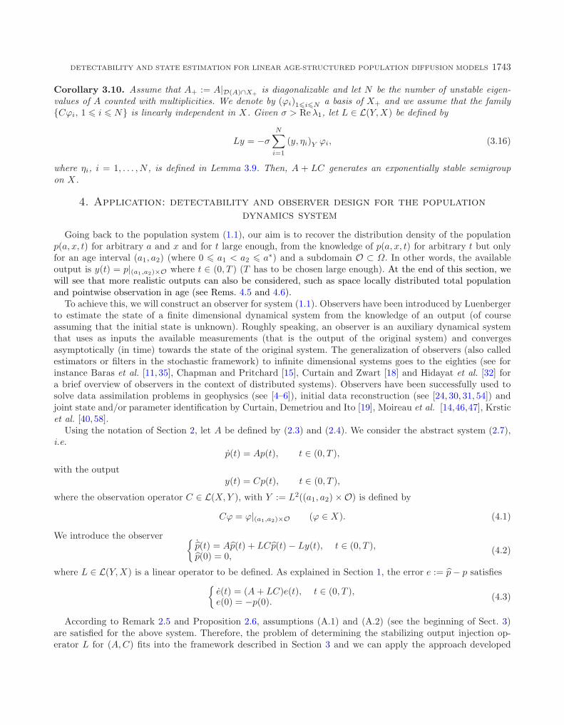
Corollary 3.10. Assume that A+ := A|D(A)∩X+ is diagonalizable and let N be the number of unstable eigen-values of A counted with multiplicities. We denote by (ϕi)1�i�N a basis of X+ and we assume that the family{Cϕi, 1 � i � N} is linearly independent in X. Given σ > Reλ1, let L ∈ L(Y,X) be defined by

Ly = −σN∑

i=1

(y, ηi)Y ϕi, (3.16)

where ηi, i = 1, . . . , N , is defined in Lemma 3.9. Then, A + LC generates an exponentially stable semigroupon X.

4. Application: detectability and observer design for the population

dynamics system

Going back to the population system (1.1), our aim is to recover the distribution density of the populationp(a, x, t) for arbitrary a and x and for t large enough, from the knowledge of p(a, x, t) for arbitrary t but onlyfor an age interval (a1, a2) (where 0 � a1 < a2 � a∗) and a subdomain O ⊂ Ω. In other words, the availableoutput is y(t) = p|(a1,a2)×O where t ∈ (0, T ) (T has to be chosen large enough). At the end of this section, wewill see that more realistic outputs can also be considered, such as space locally distributed total populationand pointwise observation in age (see Rems. 4.5 and 4.6).

To achieve this, we will construct an observer for system (1.1). Observers have been introduced by Luenbergerto estimate the state of a finite dimensional dynamical system from the knowledge of an output (of courseassuming that the initial state is unknown). Roughly speaking, an observer is an auxiliary dynamical systemthat uses as inputs the available measurements (that is the output of the original system) and convergesasymptotically (in time) towards the state of the original system. The generalization of observers (also calledestimators or filters in the stochastic framework) to infinite dimensional systems goes to the eighties (see forinstance Baras et al. [11, 35], Chapman and Pritchard [15], Curtain and Zwart [18] and Hidayat et al. [32] fora brief overview of observers in the context of distributed systems). Observers have been successfully used tosolve data assimilation problems in geophysics (see [4–6]), initial data reconstruction (see [24, 30, 31, 54]) andjoint state and/or parameter identification by Curtain, Demetriou and Ito [19], Moireau et al. [14,46,47], Krsticet al. [40, 58].

Using the notation of Section 2, let A be defined by (2.3) and (2.4). We consider the abstract system (2.7),i.e.

p(t) = Ap(t), t ∈ (0, T ),

with the outputy(t) = Cp(t), t ∈ (0, T ),

where the observation operator C ∈ L(X,Y ), with Y := L2((a1, a2) ×O) is defined by

Cϕ = ϕ|(a1,a2)×O (ϕ ∈ X). (4.1)

We introduce the observer {˙p(t) = Ap(t) + LCp(t) − Ly(t), t ∈ (0, T ),p(0) = 0,

(4.2)

where L ∈ L(Y,X) is a linear operator to be defined. As explained in Section 1, the error e := p− p satisfies{e(t) = (A+ LC)e(t), t ∈ (0, T ),e(0) = −p(0). (4.3)

According to Remark 2.5 and Proposition 2.6, assumptions (A.1) and (A.2) (see the beginning of Sect. 3)are satisfied for the above system. Therefore, the problem of determining the stabilizing output injection op-erator L for (A,C) fits into the framework described in Section 3 and we can apply the approach developed


therein. Denoting by Σ+ the set of the eigenvalues of A with non negative real part, it only remains to ver-ify the assumption of Proposition 3.5, and in particular the following lemma shows that the Hautus test ofProposition 3.5 is satisfied for our system (A,C).

Lemma 4.1. If ϕ ∈ D(A) satisfies Aϕ = λϕ for λ ∈ Σ+ and Cϕ = 0, then ϕ vanishes identically.

Proof. Let λ be an unstable eigenvalue of A (i.e. Reλ � 0) and let ϕ ∈ D(A) satisfying Aϕ = λϕ. Decomposingϕ(0, x) in the basis of L2(Ω) constituted of the eigenfunctions of the Dirichlet Laplacian (more precisely, of−kΔ), one can easily check that the unique solution of the evolution system⎧⎪⎪⎪⎪⎪⎪⎪⎨⎪⎪⎪⎪⎪⎪⎪⎩

∂ϕ

∂a(a, x) = kΔϕ(a, x) − (λ+ μ)ϕ(a, x), a ∈ (0, a∗), x ∈ Ω,

ϕ(a, x) = 0, a ∈ (0, a∗), x ∈ ∂Ω,

ϕ(0, x) =∑j∈N

αjϕDj (x), x ∈ Ω,

is given byϕ(a, x) =

∑j∈N

αje−(λ+λDj )aΠ(a)ϕD

j (x).

Plugging the above expression in the renewal equation (the last equation of (1.1)), we obtain

∑j∈N

αjϕDj (x) =

∑j∈N

αj

(∫ a∗

0

β(a)e−(λ+λDj )aΠ(a)

)ϕD

j (x).

We see that is equivalent to, for any j ∈ N, either αj = 0, either λ+ λDj solves the characteristic equation (2.2)

of the diffusion free problem. Consequently, we have

ϕ(a, x) =∑

j|λ+λDj ∈σ(A0)

αje−(λ+λDj )aΠ(a)ϕD

j (x).

The condition Cϕ = 0 reads then∑j|λ+λD

j ∈σ(A0)

αje−(λ+λDj )aϕD

j |O(x) = 0, a ∈ (a1, a2).

Since the eigenfunctions of −kΔ with Dirichlet boundary conditions are analytic, we immediately obtain thatϕ = 0. �

Remark 4.2. The above proof shows in particular that the result still holds when the diffusion coefficientdepends analytically on age.

Applying Corollary 3.6 to (4.3) immediately leads to the following result.

Theorem 4.3. Let p0 ∈ X and p the solution of (1.1). Assume that y(t) = p|(a1,a2)×O (t > 0) is known. Let pthe observer defined by (4.2), where L ∈ L(Y,X) is the (finite dimensional) stabilizing output injection operatordefined by (3.5). Then, there exist C > 0 and ω > 0 such that

‖p(t) − p(t)‖ � Ce−ωt ‖p0‖ , t > 0.


To conclude this Section, we go back to the particular but important case where the unstable system isdiagonalizable (see Sect. 3.2), i.e. we assume that A+ := A|D(A)∩X+ is diagonalizable. For the sake of simplicity,we denote here by M the number of unstable eigenvalues of A counted without multiplicities (still denoted λk,k = 1, . . . ,M) and we denote by (ϕk,i)i∈{1,...,mG

k } a basis of Ker (A−λk) where mGk is the geometric multiplicity

of λk (k = 1, . . . ,M). In order to show that the stabilizing output injection operator L can be rewritten as (3.16),it remains to verify that assumption (3.10) holds. This is done in the following lemma, which is exactly Part(A) of Claim 3.3. in ([12], p. 1458). The proof is recalled here for reader’s convenience.

Lemma 4.4. The family (Cϕk,i)1�k�M,1�i�mGk

is linearly independent in X.

Proof.

Step 1. It is easy to prove that the Hautus test (3.9), which is verified in Lemma 4.1 for A and C respectivelydefined by (2.3)−(2.4) and (4.1), is equivalent to the fact that

∀k ∈ {1, . . . ,M} , the family (Cϕk,i)1�i�mGk

is linearly independent in X.

Step 2. Consider now the case of two distinct eigenvalues, say λ1 and λ2. Assume by contradiction that thecorresponding system of eigenfunctions{

Cϕ1,i, Cϕ2,j

∣∣1 � i � mG1 , 1 � j � mG

2

}is linearly dependent and assume, for instance, that

Cϕ2,mG2

=mG

1∑i=1

αiCϕ1,i +mG

2 −1∑j=1

βjCϕ2,j ,

i.e. that

ϕ2,mG2

=mG

1∑i=1

αiϕ1,i +mG

2 −1∑j=1

βjϕ2,j on (a1, a2) ×O. (4.4)

Applying the differential operator A = −∂a − μ · +kΔ defined by (2.4), we obtain that on (a1, a2) ×O:

0 = A

⎛⎝ϕ2,mG2−

mG1∑

i=1

αiϕ1,i −mG

2 −1∑j=1

βjϕ2,j

⎞⎠ = λ2ϕ2,mG2− λ1

mG1∑

i=1

αiϕ1,i − λ2

mG2 −1∑

j=1

βjϕ2,j ,

which implies, using again (4.4) that

(λ2 − λ1)mG

1∑i=1

αiϕ1,i = 0 on (a1, a2) ×O.

Using the fact that λ1 = λ2 and Step 1, we find that αi = 0 for all i ∈ {1, . . . ,mG1

}. Therefore ϕ2,mG

2=∑mG

2 −1j=1 βjϕ2,j on (a1, a2) ×O, which contradicts Step 1.

Step 3. Finally we prove the statement of Lemma 4.4 by induction with respect to the number q � M ofdistinct eigenvalues λk. Assume that the statement holds for q−1 distinct eigenvalues λ1, . . . , λq−1 and considerthe system (Cϕk,i)1�k�q,1�i�mG

k. By contradiction, assume that this system is linearly dependent. As in Step 2,

we may assume, for instance, that

ϕq,mGq

=q−1∑k=1

mGk∑

i=1

αkiϕk,i +mG

q −1∑j=1

βjϕq,j on (a1, a2) ×O.


Applying the differential operator A and proceeding as in Step 2, we obtain that

q−1∑k=1

(λq − λk)mG

k∑i=1

αkiϕk,i = 0 on (a1, a2) ×O.

As the eigenvalues are distinct, by the inductive hypothesis, this implies that αki = 0 for any k ∈ {1, . . . , q − 1}and i ∈ {1, . . . ,mG

k

}. Therefore

ϕq,mGq

=mG

q −1∑j=1

βjϕq,j on (a1, a2) ×O,

which contradicts Step 1 and ends the proof. �

The results in this section can be extended to other observation operators, as shown in the two following remarks.

Remark 4.5. Given a1, a2 with 0 � a1 < a2 � a∗, we can take Y = L2(O) and C ∈ L(X,Y ) defined by

(Cϕ)(x) =∫ a2

a1

ϕ(a, x) da, ϕ ∈ X, x ∈ O. (4.5)

Indeed, using the third assertion in Theorem 2.4, it follows that if ϕ satisfies Aϕ = λϕ for some λ ∈ C andCϕ = 0 then there exist complex numbers αj such that

∑j|λ+λD

j ∈σ(A0)

αjϕDj (x)

∫ a2

a1

e−λ0i(j)aΠ(a) da = 0, x ∈ O,

where i(j) ∈ N∗ is the unique index such that λ0i = λ + λD

j . Using again the analyticity of the functions ϕDj ,

combined with the fact that e−λ0i(j)aΠ(a) > 0 for a ∈ [a1, a2], we conclude that ϕ = 0. The observation operator

defined in (4.5) is clearly of biological interest since measuring y = Cp signifies counting the population havingan age in the interval (a1, a2) and localized in the spatial domain O.

Remark 4.6. Another possible choice of the observation operator, which can be seen as a limit case of theoperator defined in (4.1) is

(Cϕ)(x) = ϕ(a0, x), ϕ ∈ X, x ∈ O, (4.6)

where a0 ∈ (0, a∗) is a fixed age. In this case, the conditions Aϕ = λϕ for some λ ∈ C and Cϕ = 0 write

−∂aϕ− μϕ+ kΔϕ = λϕ, ϕ ∈ D(A), (4.7)

ϕ(a0, x) = 0, x ∈ O. (4.8)

Looking to the first equation in (4.7) as a parabolic equation with a in the role of the time variable andapplying a well-known unique continuation result for parabolic equations (see, for instance, [50], Prop. 2.2) weobtain that ϕ = 0. Note that the argument used to show the observability of eigenfunctions in this case (and,consequently, for the observation operator (4.1)) can be used, without any modification, in the case μ = μ(a, x)and β = β(a, x), as assumptions (A.1) and (A.2) are satisfied in this case (see for instance [26]).


5. Discretization

From now on, we assume for the sake of simplicity that Ω is the interval (0, �), that A+ := A|D(A)∩X+ isdiagonalizable and that A has N unstable eigenvalues λ1, . . . , λN counted with multiplicities.

Our goal in the last two sections is to show how to implement the proposed method to estimate the final statefrom partial observations. More precisely, assuming that p0 is an unknown initial data, we want to estimate pat time t = T where p solves the following open loop system:⎧⎪⎪⎪⎪⎪⎪⎪⎪⎨⎪⎪⎪⎪⎪⎪⎪⎪⎩

∂tp(a, x, t) + ∂ap(a, x, t) + μ(a)p(a, x, t) − k∂xxp(a, x, t) = 0, a ∈ (0, a∗), x ∈ (0, �), t > 0,

p(a, 0, t) = p(a, �, t) = 0, a ∈ (0, a∗), t > 0,

p(a, x, 0) = p0(a, x), a ∈ (0, a∗), x ∈ (0, �),

p(0, x, t) =∫ a∗

0

β(a)p(a, x, t) da, x ∈ (0, �), t > 0,

(5.1)

provided we know the observation

y(t) = p(t)|(a1,a2)×(�1,�2), t ∈ (0, T ),

where 0 � a1 < a2 � a∗ and 0 � �1 < �2 � �.This leads to define the observation operator C ∈ L(X,Y )

Cϕ = ϕ|(a1,a2)×(�1,�2), ∀ϕ ∈ X

where X = L2((0, a∗) × (0, �)) and Y = L2((a1, a2) × (�1, �2)).In order to estimate p(T ), we use the observer designed in Section 4. As the unstable space is the

N -dimensional space (see Sect. 2),

X+ =N⊕

k=1

Ker (A− λk) = Span {ϕk, 1 � k � N}= Span

{ϕ0

i (a)ϕDj (x), λ0

i − λDj = λk, 1 � k � N

}the observer defined by (4.2) involves the stabilizing output injection operator L defined by (3.16) (see Sect. 3.2)

Ly = −σN∑

i=1

(y, ηi)Y ϕi (y ∈ Y ),

where σ > λ1 (gain coefficient) and

ηi =N∑

j=1

αijCϕj and (αij)1�i�N, 1�j�N = G−1.

(see (3.13) and (3.14)).The observer solves then the following system⎧⎪⎪⎪⎪⎪⎪⎪⎪⎪⎪⎪⎪⎪⎨⎪⎪⎪⎪⎪⎪⎪⎪⎪⎪⎪⎪⎪⎩

∂tp(a, x, t) + ∂ap(a, x, t) + μ(a)p(a, x, t) − k∂xxp(a, x, t)

+σN∑

i=1

(Cp, ηi)Y ϕi(a, x) = σ

N∑i=1

(y, ηi)Y ϕi(a, x), a ∈ (0, a∗), x ∈ (0, �), t > 0,

p(a, 0, t) = p(a, �, t) = 0, a ∈ (0, a∗), t > 0,

p(a, x, 0) = 0, a ∈ (0, a∗), x ∈ (0, �),

p(0, x, t) =∫ a∗

0

β(a)p(a, x, t) da, x ∈ (0, �), t > 0.

(5.2)


Numerical approximation of population models with spatial diffusion (typically of the form (5.1)) has beenconsidered in several papers. Lopez and Trigiante proposed in [43] an adaptative finite difference scheme to han-dle the singularity of the mortality function μ as a→ a∗. Milner [45] and Kim [38] proposed schemes using finitedifference along the characteristic age-time direction and finite elements in space or mixed finite element [39].Huyer [33] developed a semigroup approach to discretize the problem using a Galerkin approximation involv-ing Laguerre polynomials in age and spectral decomposition in space. Ayati [7] proposed a method allowingvariable time steps and independent age and time discretizations. Ayati and Dupont [8] proposed Galerkinapproximations in both age and space for a population model with nonlinear diffusion. Let us also mention thecontributions of Gerardo-Giorda et al. who proposed approximations using finite difference in age and time andfinite element in space for an age structured model with space and age dependent diffusion in [20] and densitydependent diffusion in [25]. We refer the interested reader to the Ph.D. of Pelovska [48] for more references.

Below, we successively present finite difference discretizations of systems (5.1) and (5.2). For both problems,one of the main difficulties comes from the discretization of the renewal equation p(0, x, t) =

∫ a∗

0 β(a)p(a, x, t) daappearing in the domain of the operator. Indeed, this non local equation couples the unknowns corresponding todifferent ages for a given time and at a given point of space. In [33], Huyer overcame this problem by proposinga reformulation of the system in which this condition is taken into account by adding a Dirac term in theevolution PDE defining the dynamics. Here, we use the same approach as in [20], in which the renewal equationis simplified via the time discretization: the density of population at age 0 for a given time tn is evaluated usingthe values of the density for all ages at the previous time tn−1 (see Fig. 3).

5.1. Discretization of the open loop problem: data generation

5.1.1. Rescaling the problem

In order to overcome the difficulties due to singular behavior of the coefficient μ (see Eq. (1.3)), we follow [20]and introduce the auxiliary variable

u(a, x, t) =p(a, x, t)Π(a)

= exp

(∫ a∗

0

μ(s) ds

)p(a, x, t).

One can easily check that u satisfies⎧⎪⎪⎪⎪⎪⎪⎪⎪⎨⎪⎪⎪⎪⎪⎪⎪⎪⎩

∂tu(a, x, t) + ∂au(a, x, t) − k∂xxu(a, x, t) = 0, a ∈ (0, a∗), x ∈ (0, �), t > 0,

u(a, 0, t) = u(a, �, t) = 0, a ∈ (0, a∗), t > 0,

u(a, x, 0) = u0(a, x), a ∈ (0, a∗), x ∈ (0, �),

u(0, x, t) =∫ a∗

0

m(a)u(a, x, t) da, x ∈ (0, �), t > 0,

where we have set u0(a, x) = p0(a, x)/Π(a) and where m(a) = β(a)Π(a) stands for the maternity function.

5.1.2. Finite difference discretization in time

Let un(a, x) be an approximation of u(a, x, tn), where tn = nΔt, 0 � n � Nt, Δt = T/Nt is a discretizationof (0, T ). Starting from u0(a, x) = u0(a, x), we construct un for n � 1 using an Euler’s backwards scheme⎧⎪⎪⎪⎪⎪⎪⎪⎪⎪⎨⎪⎪⎪⎪⎪⎪⎪⎪⎪⎩

1Δt

(un(a, x) − un−1(a, x)

)+ ∂au

n(a, x) − k∂xxun(a, x) = 0, a ∈ (0, a∗), x ∈ (0, �),

un(a, 0) = un(a, �) = 0, a ∈ (0, a∗),

u0(a, x) = u0(a, x), a ∈ (0, a∗), x ∈ (0, �),

un(0, x) =∫ a∗

0

m(a)un−1(a, x) da, x ∈ (0, �).


Age : k = 0, . . . , Na

Time : n = 0, . . . , Nt

k − 1 k

n − 1

n

Figure 3. Step n of the algorithm. The unknown Un,k at each node (k, n) is the vectorcontaining the solution at the different points of the space discretization.

5.1.3. Finite difference discretization in space

Denoting by uni (a) an approximation of un(xi, a) (where xi = ih = i�/(Nx + 1), with 0 � i � Nx + 1) and

using a classical centered approximation for the second order derivative in space, the above system yields⎧⎪⎪⎪⎪⎨⎪⎪⎪⎪⎩dUn

da(a) +

1h2

KUn(a) +1Δt

Un(a) =1Δt

Un−1(a),

Un(0) =∫ a∗

0

m(a)Un−1(a) da,

U0(a) = U0(a),

(5.3)

where Un(a) :=(un

1 (a), . . . , unNx

(a))T, U0(a) := (u0(a, x1), . . . , u0(a, xNx))T and

K = k

⎛⎜⎜⎜⎜⎜⎜⎝

2 −1−1 2 −1 0

−1 2 −1. . . . . . . . .

0 −1 2 −1−1 2

⎞⎟⎟⎟⎟⎟⎟⎠ .

5.1.4. Finite difference discretization in age

We use a Crank–Nicholson scheme to approximate the solution of problem (5.3). Denoting by un,ki an ap-

proximation of uni (ak), where ak = kΔa, 0 � k � Na, Δa = a∗/Na, and by Un,k =

(un,k

1 , . . . , un,kNx

)Tan

approximation of Un(ak), we move from age ak−1 to age ak following the scheme

1Δa

(Un,k − Un,k−1

)+

12h2

K(Un,k + Un,k−1

)+

12Δt(Un,k + Un,k−1

)=

12Δt(Un−1,k + Un−1,k−1

),


with the initial conditions ⎧⎪⎪⎨⎪⎪⎩U0,k = U0(ak), ∀k = 0, . . . , Na,

Un,0 =Na∑k=0

ωk m(ak)Un−1,k ∫ a∗

0

m(a)Un−1(a) da,

where ωk are the weights of the quadrature formula used.

5.1.5. Algorithm for the open loop system

(1) Initialization for n = 0: U0,k = (u0(kΔa, x1), . . . , u0(kΔa, xNh)T

(2) For n = 1, . . . , Nt:

• Initialization of Un,0 using the values of (Un−1,j): Un,0 =Na∑k=0

ωk m(ak)Un−1,k.

• For k = 1, . . . , Na, Un,k =(un,k

1 , . . . , un,kNx

)Tsolves the linear system

AUn,k = bn,k

where

A =(Δt+

12Δa

)I +

12ΔtΔa

h2K

bn,k =12Δa(Un−1,k + Un−1,k−1

)+[(Δt− 1

2Δa

)I − 1

2ΔtΔa

h2K

]Un,k−1

• Pn,k =(pn,k1 , . . . , pn,k

Nx

)Twhere pn,k

i = Π(ak)un,ki .

• Yn,k =(yn,k1 , . . . , yn,k

Nx

)Twhere yn,k

i = pn,ki if �1 � ih � �2 and yn,k

i = 0 otherwise.

5.2. Discretization of the closed loop system: observer design

In order to discretize (5.2), we follow the same procedure as in the previous subsection for the open loopsystem. The main differences in the dynamics are the presence of a source term coming from the observation yand the extra term in the evolution equation

∑Ni=1 (Cp, ηi)Y ϕi.

5.2.1. Rescaling the problem

First of all, in order to overcome the difficulties due to singular behavior of the coefficient μ, we introduce aswe did for the open loop system, the auxiliary variable

u(a, x, t) =p(a, x, t)Π(a)

= exp

(∫ a∗

0

μ(s) ds

)p(a, x, t),

where p solves (5.2).


One can easily check that u satisfies⎧⎪⎪⎪⎪⎪⎪⎪⎪⎪⎪⎪⎪⎪⎨⎪⎪⎪⎪⎪⎪⎪⎪⎪⎪⎪⎪⎪⎩

∂tu(a, x, t) + ∂au(a, x, t) − k∂xxu(a, x, t)

+σN∑

i=1

(CΠu, ηi)Y vi(a, x) = σ

N∑i=1

(y(t), ηi)Y vi(a, x), a ∈ (0, a∗), x ∈ (0, �), t > 0,

u(a, 0, t) = u(a, �, t) = 0, a ∈ (0, a∗), t > 0,

u(a, x, 0) = 0, a ∈ (0, a∗), x ∈ (0, �),

u(0, x, t) =∫ a∗

0

m(a)u(a, x, t) da, x ∈ (0, �), t > 0,

(5.4)

where we have set vi(a, x) = ϕi(a, x)/Π(a) (1 � i � N).In order to discretize the term (CΠu, ηi)Y in (5.4), let us introduce the new (scalar) unknowns

θi(t) = (CΠu, ηi)Y (1 � i � N).

Using the first equation in (5.4) and the fact that, for any i, j ∈ {1, . . . , N},

(CΠvj , ηi)Y = (Cϕj , ηi)Y =N∑

k=1

αik (Cϕj , Cϕk)Y =N∑

k=1

αik (Cϕk, Cϕj)Y = δij ,

(by (3.13) and (3.14)), we remark that θi satisfies

θi(t) = − (CΠ∂au, ηi)Y + k (CΠ∂xxu, ηi)Y − σθi(t) + σ (y, ηi)Y .

Consequently, problem (5.4) can be reformulated as follows⎧⎪⎪⎪⎪⎪⎪⎪⎪⎪⎪⎪⎪⎪⎪⎪⎪⎪⎪⎪⎪⎪⎪⎪⎪⎪⎨⎪⎪⎪⎪⎪⎪⎪⎪⎪⎪⎪⎪⎪⎪⎪⎪⎪⎪⎪⎪⎪⎪⎪⎪⎪⎩

θi(t) = − (CΠ∂au(t), ηi)Y + k (CΠ∂xxu(t), ηi)Y

−σθi(t) + σ (y(t), ηi)Y , t > 0, 1 � i � N,

∂tu(a, x, t) + ∂au(a, x, t) − k∂xxu(a, x, t) + σ

N∑i=1

θi(t)vi(a, x)

= σ

N∑i=1

(y(t), ηi)Y vi(a, x), a ∈ (0, a∗), x ∈ (0, �), t > 0,

θi(0) = 0, 1 � i � N,

u(a, 0, t) = u(a, �, t) = 0, a ∈ (0, a∗), t > 0,

u(a, x, 0) = 0, a ∈ (0, a∗), x ∈ (0, �),

u(0, x, t) =∫ a∗

0

m(a)u(a, x, t) da, x ∈ (0, �), t > 0.

5.2.2. Finite difference discretization in time

Let un(a, x) (resp. θni , yn(a, x)) be an approximation of u(a, x, tn) (resp. θi(tn), y(a, x, tn)), where tn = nΔt,

0 � n � Nt, Δt = T/Nt is a discretization of (0, T ). Starting from θ0i = 0 and u0(a, x) = 0, we construct θni


and un for n � 1 using an Euler’s backwards scheme⎧⎪⎪⎪⎪⎪⎪⎪⎪⎪⎪⎪⎪⎪⎪⎪⎪⎪⎪⎪⎪⎪⎪⎪⎪⎨⎪⎪⎪⎪⎪⎪⎪⎪⎪⎪⎪⎪⎪⎪⎪⎪⎪⎪⎪⎪⎪⎪⎪⎪⎩

1Δt

(θn

i − θn−1i

)= − (CΠ∂au

n−1, ηi

)Y

+ k(CΠ∂xxu

n−1, ηi

)Y

−σθni + σ (yn, ηi)Y , 1 � i � N,

1Δt

(un(a, x) − un−1(a, x)

)+ ∂au

n(a, x) − k∂xxun(a, x)

+σN∑

i=1

θni vi(a, x) = σ

N∑i=1

(yn, ηi)Y vi(a, x), a ∈ (0, a∗), x ∈ (0, �),

θ0i = 0, 1 � i � N,

un(a, 0) = un(a, �) = 0, a ∈ (0, a∗),

u0(a, x) = 0, a ∈ (0, a∗), x ∈ (0, �),

un(0, x) =∫ a∗

0

m(a)un−1(a, x) da, x ∈ (0, �).

5.2.3. Finite difference discretization in space

Denoting by uni (a) an approximation of un(xi, a) (where xi = ih = i�/(Nx + 1), with 0 � i � Nx + 1) and

using a classical centered approximation for the second order derivative in space, the above system yields⎧⎪⎪⎪⎪⎪⎪⎪⎪⎪⎪⎪⎪⎪⎪⎪⎪⎪⎪⎪⎪⎪⎪⎪⎨⎪⎪⎪⎪⎪⎪⎪⎪⎪⎪⎪⎪⎪⎪⎪⎪⎪⎪⎪⎪⎪⎪⎪⎩

1Δt

θni =

1Δt

θn−1i − σθn

i − h

(∫ a2

a1

Π(a)ηi(a)T∂aUn−1(a) da

)− 1h

(∫ a2

a1

Π(a)ηi(a)TKUn−1(a) da

)+ σh

(∫ a2

a1

ηi(a)TYn(a) da

),

dUn

da(a) +

1h2

KUn(a) +1Δt

Un(a) + σ

N∑i=1

θni Vi(a) =

1Δt

Un−1(a)

+σhN∑

i=1

(∫ a2

a1

ηi(a)TYn(a) da

)Vi(a),

θ0i = 0,

Un(0) =∫ a∗

0

m(a)Un−1(a) da,

U0(a) = 0,

(5.5)

where

Un(a) :=(un

1 (a), . . . , unNx

(a))T

Vi(a) := (vi(a, x1), . . . , vi(a, xNx))T ,

ηi(a) := (ηi(a, x1), . . . , ηi(a, xNx))T , Yn(a) := (yn(a, x1), . . . , yn(a, xNx))T .

We take here yn(a, xi) = 0 for all i ∈ {1, . . . , Nx} such that xi /∈ (�1, �2), for all a ∈ (0, a∗) and all n � 1.

5.2.4. Finite difference discretization in age

We use a Crank–Nicholson scheme to approximate the solution of problem (5.5). Denoting by un,ki an ap-

proximation of uni (ak), where ak = kΔa, 0 � k � Na, Δa = a∗/Na, Na1 = �a1/Δa�, Na2 = �a2/Δa� and by


Un,k :=(un,k

1 , . . . , un,kNx

)Tan approximation of Un(ak), we move from age ak−1 to age ak following the scheme

1Δt

θni =

1Δt

θn−1i − σθn

i − hΔa

⎛⎝ Na2∑k=Na1

Π(kΔa)(ηk

i

)T(Un−1,k − Un−1,k−1

Δa

)⎞⎠− Δa

h

⎛⎝ Na2∑k=Na1

Π(kΔa)(ηk

i

)TKUn−1,k

⎞⎠+ σhΔa

⎛⎝ Na2∑k=Na1

(ηk

i

)TYn,k

⎞⎠ ,and

1Δa

(Un,k − Un,k−1

)+

12h2

K

(Un,k + Un,k−1

)+

12Δt

(Un,k + Un,k−1

)+ σ

N∑i=1

θni Vk

i

=1

2Δt

(Un−1,k + Un−1,k−1

)+ σhΔa

N∑i=1

⎛⎝ Na2∑j=Na1

(ηj

i

)TYn,j

⎞⎠Vki ,

with the initial conditions ⎧⎪⎪⎪⎪⎪⎪⎨⎪⎪⎪⎪⎪⎪⎩

θ0i = 0, ∀i = 1, . . . , N,

U0,k = 0, ∀k = 0, . . . , Na,

Un,0 =Na∑k=0

ωk m(ak)Un−1,k.

Here: Vki := (vi(kΔa, x1), . . . , vi(kΔa, xNx)T, ηk

i := (ηi(kΔa, x1), . . . , ηi(kΔa, xNx))T , and Yn,k :=(yn(kΔa, x1), cyn(kΔa, xNx)))T.

5.2.5. Algorithm for the observer

(1) For n = 0 : Initialization of θ0i (1 � i � N) and U0,k (k = 0, . . . , Na) at 0.(2) For n = 1, . . . , Nt :

• Calculate θni using the values of θn−1

i and (Un−1,j)Na2j=Na1−1:

θni =

11 + σΔt

⎛⎝θn−1i − hΔt

Na2∑k=Na1

Π(kΔa)(ηk

i

)T (Un−1,k − Un−1,k−1

)

−ΔaΔth

Na2∑k=Na1

Π(kΔa)(ηk

i

)TKUn−1,k + σhΔaΔt

Na2∑k=Na1

(ηk

i

)TYn,k

⎞⎠• k = 0: Initialization of Un,0 using the values of (Un−1,j)Na

j=0:

Un,0 =Na∑k=0

ωk m(kΔa)Un−1,k

• For k = 1, . . . , Na, solve the linear system

AUn,k = bn,k


Age : k = 0, . . . , Na

θn

θn−1

Un,kUn,0

Time : n = 0, . . . , Nt

k − 1 k

n − 1

n

Figure 4. Step n of the algorithm. First, θni is computed using θn−1

i and Un−1,k, for k =Na1 − 1, . . . , Na2 (pink arrows). Next, Un,0 is deduced from Un−1,k, for k = 0, . . . , Na. Finally,Un,k for k � 1 is computed using θn

i , Un,k−1, Un−1,k and Un−1,k−1 (blue arrows). (Coloronline)

where

A =(Δt+

12Δa

)I +

12ΔtΔa

h2K

bn,k =12Δa(Un−1,k + Un−1,k−1

)+[(Δt− 1

2Δa

)I − 1

2ΔtΔa

h2K

]Un,k−1

− σΔaΔt

N∑i=1

θni Vk

i + σh(Δa)2ΔtN∑

i=1

⎛⎝ Na2∑j=Na1

(ηj

i

)TYn,j

⎞⎠Vki

• Pn,k =(pn,k1 , . . . , pn,k

Nx

)Twhere pn,k

i = Π(ak)un,ki .

6. Numerical results

We present in this section some numerical results illustrating the efficiency of our state reconstruction method.All the numerical tests are two-dimensional and run on Matlab.Taking a∗ = 2, we choose the fertility function to be (see Fig. 5)

β(a) = 10 a(a∗ − a) exp{−20(a− a∗/3)2

},

while the mortality function is chosen asμ(a) = (a∗ − a)−1.

Note that for this particular choice of μ, the function Π(a) can be computed explicitly:

Π(a) = exp(−∫ a

0

μ(s) ds)

=a∗ − a

a∗·


0 0.2 0.4 0.6 0.8 1 1.2 1.4 1.6 1.8 20

2

4

6

8

10

12

14

Fertility functionMortality function

Figure 5. The fertility and mortality functions.

Figure 6. Initial state corresponding to the first eigenfunction (3D and 2D representations).

6.1. Distributed observation in space and full observation in age

We take Ω = (0, π) (i.e. � = π), and we consider full observation in age (i.e. (a1, a2) = (0, a∗)) and partialobservation in space : (�1, �2) = (�/3, 2�/3). The time of observation is T = 2a∗ and the diffusion coefficient isk = 1. Under these assumptions, there is a unique unstable eigenvalue λ1 = λ0

1 − 1, where λ01 is the unique real

solution of the characteristic equation (2.2). Computing numerically this value, we obtain that λ1 = 0.239.We first choose as initial state an eigenfunction corresponding to the (unique) unstable eigenvalue λ1 (see

Fig. 6), i.e. we take

p0(a, x) = ϕ1(a, x) = ϕ01(a)ϕ

D1 (x) =

a∗ − a

a∗e−λ0

1a sin(x). (6.1)


Figure 7. Estimated (left) and exact (right) solution at time t = T .

Figure 8. Gaussian initial state (3D and 2D representations).

The solution of problem (5.1) is then simply given by

p(a, x, t) = eλ1tp0(a, x).

To validate our reconstruction method, we first generate numerically an output by solving problem (5.1) withp0 given by (6.1). To avoid committing an “inverse crime” ([16], p. 154), we use different space discretizationsto generate the measurement and in the reconstruction step.

Using Nx = 100 points of discretization in space, Na = 120 points in discretization in age and a time stepΔt = Δa/2, we obtain an L2 relative error of 4.07% (see Fig. 7 for a representation of the estimated and exactsolutions). In this numerical test, the gain coefficient is chosen as σ = 2 + λ1.

From now on, we consider the more realistic situation of noisy observation and gaussian type initial data ofthe form (see Fig. 8)

p0(a, x) = exp{− (30(a− a∗/4)2 + 20(x− �/4)2

)}.

Using the same discretization parameters, we obtain an L2 relative error of 2.99% with 5% of noise, 9.6% with10% of noise and 16.3% with 15% of noise; see Figure 9 for a representation of the estimated and exact solutionsat time t = T in the case of 5% of noise. Figure 10 shows the decay of the state error with time.


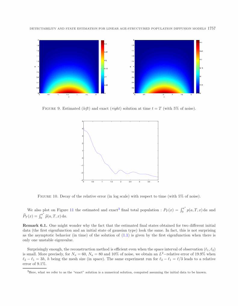
Figure 9. Estimated (left) and exact (right) solution at time t = T (with 5% of noise).

0 0.5 1 1.5 2 2.5 3 3.5 4−3

−2

−1

0

1

2

3

4

5

Figure 10. Decay of the relative error (in log scale) with respect to time (with 5% of noise).

We also plot on Figure 11 the estimated and exact3 final total population : PT (x) =∫ a∗

0 p(a, T, x) da and

PT (x) =∫ a∗

0p(a, T, x) da.

Remark 6.1. One might wonder why the fact that the estimated final states obtained for two different initialdata (the first eigenfunction and an initial state of gaussian type) look the same. In fact, this is not surprisingas the asymptotic behavior (in time) of the solution of (1.1) is given by the first eigenfunction when there isonly one unstable eigenvalue.

Surprisingly enough, the reconstruction method is efficient even when the space interval of observation (�1, �2)is small. More precisely, for Nx = 60, Na = 80 and 10% of noise, we obtain an L2−relative error of 19.9% when�2 − �1 = 3h, h being the mesh size (in space). The same experiment run for �2 − �1 = �/3 leads to a relativeerror of 9.1%.

3Here, what we refer to as the “exact” solution is a numerical solution, computed assuming the initial data to be known.


0 0.5 1 1.5 2 2.5 3 3.50

0.02

0.04

0.06

0.08

0.1

0.12

0.14

0.16

0.18

EstimatedExact

0 0.5 1 1.5 2 2.5 3 3.50

0.02

0.04

0.06

0.08

0.1

0.12

0.14

0.16

0.18

0.2

EstimatedExact

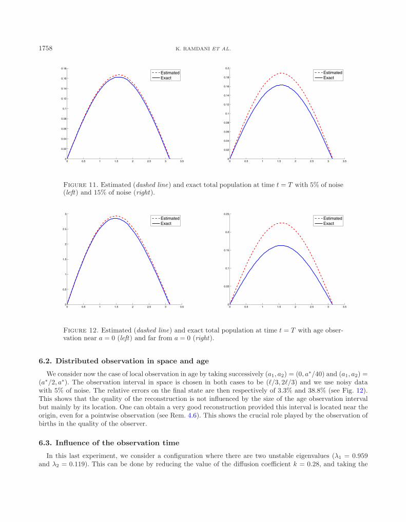
Figure 11. Estimated (dashed line) and exact total population at time t = T with 5% of noise(left) and 15% of noise (right).

0 0.5 1 1.5 2 2.5 3 3.50

0.5

1

1.5

2

2.5

3

EstimatedExact

0 0.5 1 1.5 2 2.5 3 3.50

0.05

0.1

0.15

0.2

0.25

EstimatedExact

Figure 12. Estimated (dashed line) and exact total population at time t = T with age obser-vation near a = 0 (left) and far from a = 0 (right).

6.2. Distributed observation in space and age

We consider now the case of local observation in age by taking successively (a1, a2) = (0, a∗/40) and (a1, a2) =(a∗/2, a∗). The observation interval in space is chosen in both cases to be (�/3, 2�/3) and we use noisy datawith 5% of noise. The relative errors on the final state are then respectively of 3.3% and 38.8% (see Fig. 12).This shows that the quality of the reconstruction is not influenced by the size of the age observation intervalbut mainly by its location. One can obtain a very good reconstruction provided this interval is located near theorigin, even for a pointwise observation (see Rem. 4.6). This shows the crucial role played by the observation ofbirths in the quality of the observer.

6.3. Influence of the observation time

In this last experiment, we consider a configuration where there are two unstable eigenvalues (λ1 = 0.959and λ2 = 0.119). This can be done by reducing the value of the diffusion coefficient k = 0.28, and taking the


0 0.5 1 1.5 2 2.5 3 3.50

0.05

0.1

0.15

0.2

0.25

0.3

0.35

0.4

0.45

0.5

EstimatedExact

0 0.5 1 1.5 2 2.5 3 3.5−0.05

0

0.05

0.1

0.15

0.2

0.25

0.3

EstimatedExact

Figure 13. Estimated (dashed line) and exact total population at time t = T , for T = a∗(left) and for T = 0.5a∗ (right).

same parameters as in the previous numerical test. The observation interval in space is chosen to be (�/3, 2�/3)and (a1, a2) = (0, a∗/20).

For T = a∗, the observer yields a good approximation of the final state (the relative error is 3.83%), andan even better approximation of the total population (the relative error is 1.81%). For an observation timeT = 0.5a∗, the estimate provided by the observer is not very accurate, the relative error being 27%. However,we still obtain a reasonable approximation of the total population, as it can be seen from Figure 13.

References

[1] B. Ainseba, Exact and approximate controllability of the age and space population dynamics structured model. J. Math. Anal.Appl. 275 (2002) 562–574.

[2] B. Ainseba and M. Iannelli, Exact controllability of a nonlinear population-dynamics problem. Differ. Integral Equ. 16 (2003)1369–1384.

[3] B. Ainseba and M. Langlais, On a population dynamics control problem with age dependence and spatial structure. J. Math.Anal. Appl. 248 (2000) 455–474.

[4] D. Auroux and J. Blum, Back and forth nudging algorithm for data assimilation problems. C. R. Acad. Sci. Paris Ser. I Math.340 (2005) 873–878.

[5] D. Auroux and M. Nodet, The back and forth nudging algorithm for data assimilation problems: theoretical results on transportequations. ESAIM: COCV 18 (2012) 318–342.

[6] D. Auroux, P. Bansart and J. Blum, An evolution of the back and forth nudging for geophysical data assimilation: applicationto Burgers equation and comparisons. Inverse Probl. Sci. Eng. 21 (2013) 399–419.

[7] B.P. Ayati, A variable time step method for an age-dependent population model with nonlinear diffusion. SIAM J. Numer.Anal. 37 (2000) 1571–1589.

[8] B.P. Ayati and T.F. Dupont, Galerkin methods in age and space for a population model with nonlinear diffusion. SIAM J.Numer. Anal. 40 (2002) 1064–1076.

[9] M. Badra and T. Takahashi, Stabilization of parabolic nonlinear systems with finite dimensional feedback or dynamicalcontrollers: application to the Navier-Stokes system. SIAM J. Control Optim. 49 (2011) 420–463.

[10] M. Badra and T. Takahashi, On the Fattorini criterion for approximate controllability and stabilizability of parabolic systems.ESAIM: COCV 20 (2014) 924–956.

[11] J.S. Baras, A. Bensoussan and M.R. James, Dynamic observers as asymptotic limits of recursive filters: special cases. SIAMJ. Appl. Math. 48 (1988) 1147–1158.

[12] V. Barbu and R. Triggiani, Internal stabilization of Navier-Stokes equations with finite-dimensional controllers. Indiana Univ.Math. J. 53 (2004) 1443–1494.

[13] W.L. Chan and B.Z. Guo, On the semigroups of age-size dependent population dynamics with spatial diffusion. Manuscr.Math. 66 (1989) 161–181.

[14] D. Chapelle, N. Cındea and P. Moireau, Improving convergence in numerical analysis using observers—the wave-like equationcase. Math. Models Methods Appl. Sci. 22 (2012) 1250040.


[15] M.J. Chapman and A.J. Pritchard, Finite-dimensional compensators for nonlinear infinite-dimensional systems, in Controltheory for distributed parameter systems and applications (Vorau, 1982). Vol. 54 of Lect. Notes Control Inform. Sci. Springer,Berlin (1983) 60–76.

[16] D. Colton and R. Kress, Inverse acoustic and electromagnetic scattering theory. Vol. 93 of Appl. Math. Sci., 2nd edition.Springer-Verlag, Berlin, (1998).

[17] J.-M. Coron and E. Trelat, Global steady-state controllability of one-dimensional semilinear heat equations. SIAM J. ControlOptim. 43 (2004) 549–569.

[18] R.F. Curtain and H. Zwart, An introduction to infinite-dimensional linear systems theory. Vol. 21 of Texts Appl. Math.Springer-Verlag, New York (1995).

[19] R. Curtain, M. Demetriou and K. Ito, Adaptive observers for structurally perturbed infinite dimensional systems, in Proc. ofthe 36th IEEE Conference on Decision and Control, 1997, Vol. 1 (1997) 509–514.

[20] C. Cusulin and L. Gerardo-Giorda, A numerical method for spatial diffusion in age-structured populations. Numer. MethodsPartial Differ. Equ. 26 (2010) 253–273.

[21] G. Di Blasio and A. Lorenzi, Direct and inverse problems in age-structured population diffusion. Discrete Contin. Dyn. Syst.Ser. S 4 (2011) 539–563.

[22] G. Di Blasio and A. Lorenzi, An identification problem in age-dependent population diffusion. Numer. Funct. Anal. Optim.34 (2013) 36–73.

[23] H.W. Engl, W. Rundell and O. Scherzer, A regularization scheme for an inverse problem in age-structured populations. J.Math. Anal. Appl. 182 (1994) 658–679.

[24] E. Fridman, Observers and initial state recovering for a class of hyperbolic systems via Lyapunov method. Automatica 49(2013) 2250–2260.

[25] L. Gerardo-Giorda, Numerical approximation of density dependent diffusion in age-structured population dynamics, in Con-ference Applications of Mathematics 2013 in honor of the 70th birthday of Karel Segeth, edited by J. Brandts, S. Korotov,M. Kryzek, J. Sistek and T. Vejchodsky. Vol. 2013. Institute of Mathematics AS CR, Prague (2013) 88–97.

[26] B.Z. Guo and W.L. Chan, On the semigroup for age dependent population dynamics with spatial diffusion. J. Math. Anal.Appl. 184 (1994) 190–199.

[27] M.E. Gurtin, A system of equations for age-dependent population diffusion. J. Theoret. Biol. 40 (1973).

[28] M.E. Gurtin and R.C. MacCamy, Diffusion models for age-structured populations. Math. Biosci. 54 (1981) 49–59.

[29] M. Gyllenberg, A. Osipov and L. Paivarinta, The inverse problem of linear age-structured population dynamics. J. Evol. Equ.2 (2002) 223–239.

[30] G. Haine, Recovering the observable part of the initial data of an infinite-dimensional linear system with skew-adjoint generator.Math. Control. Signals Syst. 26 (2014) 435–462.

[31] G. Haine and K. Ramdani, Reconstructing initial data using observers: error analysis of the semi-discrete and fully discreteapproximations. Numer. Math. 120 (2012) 307–343.

[32] Z. Hidayat, R. Babuska, B. De Schutter and A. Nunez, Observers for linear distributed-parameter systems: A survey, in IEEEInternational Symposium on, Robotic and Sensors Environments (ROSE) (2011) 166–171.

[33] W. Huyer, Semigroup formulation and approximation of a linear age-dependent population problem with spatial diffusion.Semigroup Forum 49 (1994) 99–114.

[34] W. Huyer, Approximation of a linear age-dependent population model with spatial diffusion. Commun. Appl. Anal. 8 (2004)87–108.

[35] M.R. James and J.S. Baras, An observer design for nonlinear control systems, in Analysis and optimization of systems (Antibes,1988). Vol. 111 of Lect. Notes Control Inform. Sci. Springer, Berlin (1988) 170–180.

[36] T. Kato, Perturbation theory for linear operators. Classics in Mathematics. Springer-Verlag, Berlin (1995).

[37] O. Kavian and O. Traore, Approximate controllability by birth control for a nonlinear population dynamics model. ESAIM:COCV 17 (2011) 1198–1213.

[38] M.-Y. Kim, Galerkin methods for a model of population dynamics with nonlinear diffusion. Numer. Methods Partial Differ.Equ. 12 (1996) 59–73.

[39] M.-Y. Kim and E.-J. Park, Mixed approximation of a population diffusion equation. Comput. Math. Appl. 30 (1995) 23–33.

[40] M. Krstic, L. Magnis and R. Vazquez, Nonlinear control of the viscous Burgers equation: Trajectory generation, tracking andobserver design. J. Dyn. Syst. Meas. Control 131 (2009) 021012.

[41] M. Langlais, A nonlinear problem in age-dependent population diffusion. SIAM J. Math. Anal. 16 (1985) 510–529.

[42] M. Langlais, Large time behavior in a nonlinear age-dependent population dynamics problem with spatial diffusion J. Math.Biol. 26 (1988) 319–346.

[43] L. Lopez and D. Trigiante, A finite difference scheme for a stiff problem arising in the numerical solution of a populationdynamic model with spatial diffusion. Nonlin. Anal. 9 (1985) 1–12.

[44] D. Luenberger, Observing the state of a linear system, IEEE Trans. Mil. Electron. MIL-8 (1964) 74–80.

[45] F.A. Milner, A numerical method for a model of population dynamics with spatial diffusion. Comput. Math. Appl. 19 (1990)31–43.

[46] P. Moireau, D. Chapelle and P. Le Tallec, Joint state and parameter estimation for distributed mechanical systems. Comput.Methods Appl. Mech. Eng. 197 (2008) 659–677.

[47] P. Moireau, D. Chapelle and P. Le Tallec, Filtering for distributed mechanical systems using position measurements: perspec-tives in medical imaging Inverse Probl. 25 (2009) 035010.


[48] G.G. Pelovska, Numerical investigations in the field of age-structured population dynamics. Ph.D. thesis, University of Trento(2007).

[49] A. Perasso, Identifiabilite de parametres pour des systemes decrits par des equations aux derivees partielles. Application a ladynamique des populations. Ph.D. thesis, Universite Paris Sud XI (2009).

[50] K.D. Phung and G. Wang, An observability estimate for parabolic equations from a measurable set in time and its applications.J. Eur. Math. Soc. 15 (2013) 681–703.

[51] M. Pilant and W. Rundell, Determining a coefficient in a first-order hyperbolic equation. SIAM J. Appl. Math. 51 (1991)494–506.

[52] J.-P. Puel, Une approche non classique d’un probleme d’assimilation de donnees. C. R. Math. Acad. Sci. Paris 335 (2002)161–166.

[53] J.-P. Puel, A nonstandard approach to a data assimilation problem and Tychonov regularization revisited. SIAM J. ControlOptim. 48 (2009) 1089–1111.

[54] K. Ramdani, M. Tucsnak and G. Weiss, Recovering the initial state of an infinite-dimensional system using observers. Auto-matica 46 (2010) 1616–1625.

[55] J.-P. Raymond and L. Thevenet, Boundary feedback stabilization of the two dimensional Navier-Stokes equations with finitedimensional controllers. Discrete Contin. Dyn. Syst. 27 (2010) 1159–1187.

[56] A. Rhandi, Positivity and stability for a population equation with diffusion on L1. Positivity 2 (1998) 101–113.

[57] W. Rundell, Determining the death rate for an age-structured population from census data. SIAM J. Appl. Math. 53 (1993)1731–1746.

[58] A. Smyshlyaev and M. Krstic, Backstepping observers for a class of parabolic PDEs. Syst. Control Lett. 54 (2005) 613–625.

[59] J. Song, J.Y. Yu, X.Z. Wang, S.J. Hu, Z.X. Zhao, J.Q. Liu, D.X. Feng and G.T. Zhu, Spectral properties of population operatorand asymptotic behaviour of population semigroup. Acta Math. Sci. 2 (1982) 139–148.

[60] O. Traore, Null controllability of a nonlinear population dynamics problem. Int. J. Math. Math. Sci. 20 (2006) 49279.

[61] O. Traore, Approximate controllability and application to data assimilation problem for a linear population dynamics model.Int. J. Appl. Math. 37 (2007) 1, 12.

[62] O. Traore, Null controllability and application to data assimilation problem for a linear model of population dynamics. Ann.Math. Blaise Pascal 17 (2010) 375–399.

[63] R. Triggiani, On the stabilizability problem in Banach space. J. Math. Anal. Appl. 52 (1975) 383–403.

[64] R. Triggiani, Addendum. J. Math. Anal. Appl. 56 (1976) 492-493.

[65] R. Triggiani, Boundary feedback stabilizability of parabolic equations. Appl. Math. Optim. 6 (1980) 201–220.

[66] C. Walker, Some remarks on the asymptotic behavior of the semigroup associated with age-structured diffusive populations.Monatsh. Math. 170 (2013) 481–501.

[67] G.F. Webb, Theory of nonlinear age-dependent population dynamics. Vol. 89 of Monogr. Textb. Pure Appl. Math. MarcelDekker, Inc., New York (1985).

[68] G.F. Webb, Population models structured by age, size and spatial position, in Structured population models in biology andepidemiology. Vol. 1936 of Lect. Notes Math. Springer, Berlin (2008) 1–49.

[69] J. Zabczyk, Remarks on the algebraic Riccati equation in Hilbert space. Appl. Math. Optim. 2 (1975/76) 251–258.

detectability and state estimation for linear age

Documents