Chapter 4

Linear Estimation Theory

• Virtually all branches of science, engineering, and social science for data analysis, sys-tem control subject to random disturbances or for decision making based on incompleteinformation call for estimation theory.

• Many estimation problem can be formulated as a minimum norm problem in Hilbertspace.

• The projection theorem can be applied directly to the area of statistical estimation.

• There are a number of different ways to formulate a statistical estimation.

¦ Least squares.

¦ Maximum likelihood

¦ Bayesian techniques.

• When all variables are Gaussian statistics, these techniques produce linear equations.

103

104 CHAPTER 4. LINEAR ESTIMATION THEORY

Preliminaries

• If x is a real-valued random variable,

¦ The probability distribution P of the variable x is defined to be

P (ξ) = Prob(x ≤ ξ).

¦ The “derivative” p(ξ) of the probability distribution P (ξ) is called the probabilitydensity function (pdf) of the variable x, i.e.,

P (ξ) =

∫ ξ

−∞

p(x)dx.

. Note that ∫ ∞

−∞

p(x)dx = 1.

. p(ξ) ≥ 0 for all ξ.

• The expected value of any function g of x is defined to be

E [g(x)] :=

∫ ∞

−∞

g(ξ)p(ξ)dξ.

¦ The expected value of x is E [x].

¦ The variance of x is E [(x− E [x])2].

105

• For random vector x = [x1, . . . , xn]>,

¦ There is a joint probability distribution P defined by

P (ξ1, . . . ξn) = Prob(x1 ≤ ξ1, . . . , xn ≤ ξn).

¦ The covariance matrix cov(x) is defined by

cov(x) = E[(x− E [x])(x− E [x])>

].

. Two random variables xi and xj are said to be uncorrelated or stochasticallyindependent if

E [(x1 − E [x1])(x2 − E [x2])] = E [x1 − E [x1]]E [x2 − E [x2]].

106 Estimation

Least Squares Model

• This is a familiar subject as we have seen in many occasions.

• This problem is not a statistical one.

• It amounts to approximating a vector y ∈ Rm by a vector lying in the column space ofW ∈ Rm×n and n < m.

¦ We assume a linear model that the response y is related to the input β linearly, i.e.,

y =Wβ.

¦ We would like to recover β from observed y. (Would it be a linear relationship?)

¦ We are not assuming that the observed y carries errors.

• It would be interesting to compare the least squares setting with those with randomnoises.

Least Squares Model 107

Least Squares Formulation

• Given

¦ A known matrix W ∈ Rm×n, n < m.

¦ An observation vector y ∈ Rm.

Find β ∈ Rn such that ‖y −W β‖ is minimized over all β ∈ Rn.

• By the projection theorem, the solution exists and is unique.

• The normal equation is given by

W>(y −W β) = 0.

• If W has linear independent columns, then

β = (W>W )−1W>

︸ ︷︷ ︸

K

y.

¦ Note that the optimal solution β is related to y linearly.

108 Estimation

Gauss-Markov Model

• A more realistic model in an experiment is

y =Wβ + ε.

¦ W ∈ Rm×n is known.

¦ ε ∈ Rm is a random vector with zero mean and covariance E(εε>) = Q.

¦ y represents the outcome of inexact measurements in Rm.

• Want to estimate unknown parameter vector β ∈ Rn from y ∈ Rm using

β := Ky

with K an unknown matrix in Rn×m.

• Suppose the approximation is measured by minimizing the expected value of the error,i.e.,

minK∈Rn×m

E [‖β − β‖2]

¦ Since y carries random noise, it is a random vector.

¦ Both estimate β and the difference β − β are random vectors.

¦ The statistics of these random vectors are determined by those of ε and K.

Gauss-Markov Model 109

Gauss-Markov Estimate

• Observe that

E [‖β − β‖2] = E [〈K(Wβ + ε)− β, K(Wβ + ε)− β〉]

= ‖KWβ − β‖2 + E [〈Kε,Kε〉].

• Consider unbiased estimation:

¦ ObserveE [β] = E [KWβ +Kε] = KWE [β].

It is expected that KW = In.

¦ The problem now becomes, given a symmetric and positive definite matrix Q,

minimizeK∈Rn×m trace KQK>

subject to KW = In.

¦ This is in the form of a standard minimum norm problem.

110 Estimation

• The problem has a closed form solution.

¦ The optimal solution is given by

K =(W>Q−1W

)−1W>Q−1.

¦ The minimum-variance unbiased estimation of β is given by

β =(W>Q−1W

)−1W>Q−1y.

¦ The special case Q = Im is the classical least squares problem.

. The classical least squares solution is providing the unbiased minimum-varianceestimate of β, if the perturbation presented in data is white noise.

• It can be argued that the above solution βi is the minimum-variance unbiased estimationof βi for each individual i.

¦ This is the true minimum-variance unbiased estimate.

Minimum-Variance Model 111

Minimum-Variance Model

• Assume in the linear modely =Wβ + ε.

¦ W ∈ Rm×n is known.

¦ ε ∈ Rm is a random vector with zero mean and covariance E(εε>) = Q.

¦ β is a random vector in Rn with known statistical information.

¦ y represents the outcome of inexact measurements in Rm.

• Want to estimate the unknown random vector β ∈ Rn based on y ∈ Rm using

β := Ky

where K is an unknown matrix in Rn×m.

• The best approximation is measured by minimizing the expected value of the randomerror, i.e.,

minK∈Rn×m

E [‖β − β‖2]

112 Estimation

Minimum-Variance Estimate

• Assume (E [yyT ])−1 exists. Then the minimum-variance estimator of β is given by

β = E [βyT ](E [yyT ])−1y.

¦ The estimate is independent of W and ε.

• Proof Is Interesting!

¦ Write K in rows, i.e., K = [k>1 , . . .k>n ]>.

¦ E [‖β − β‖2] =∑n

i=1 E [(βi − βi)2] =

∑n

i=1 E [(k>i y − βi)

2].

. Suffices to consider each individual term.

¦ Let f(y, βi) denote the (unknown) joint pdf of y and βi.

. Define

g(ki) := E [(y>ki − βi)2]

=

∫ ∫

(y>ki − βi)2f(y, βi) dy dβi.

. Necessary condition is ∇g(ki) = 0.

Minimum-Variance Model 113

¦ Easy to see

∂g

∂ki,j=

∫ ∫

2(y>ki − βi)yjf(y, βi) dy dβi

= 2E [(y>ki − βi)yj].

¦ Rewrite the necessary condition as

E [y(y>ki − βi)] = 0, (for each i)

E [yy>]K> = E [yβ>], (in matrix form)

K = E [βy>](E [yy>])−1.

• The estimate so far is biased, unless E [β] = E [y] = 0.

• In the general case where E [β] = β0 and E [y] = y0,

¦ The estimate should assume the form

β := Ky + b.

¦ The minimum-variance estimate is given by

β = β0 + E [(β − β0)(y − y0)>](E [(y − y0)(y − y0)

>])−1(y − y0).

114 Estimation

Equivalent Formulas

• Assume that

E [εε>] = Q ∈ Rm×m,

E [ββ>] = R ∈ Rn×n,

E [εβ>] = 0 ∈ Rm×n.

• Then the minimum-variance estimate can be written as

β = RW>(WRW> +Q)−1︸ ︷︷ ︸

K

y

=

K︷ ︸︸ ︷

(W>Q−1W +R−1)−1W>Q−1 y.

¦ The equivalence can be proved by direct substitution.

¦ Check out the dimension of the inverse matrices involved in the two expressions.

Minimum-Variance Model 115

Comparision with Gauss-Markov Estimate

• The Gauss-Markov estimate is

β =(W>Q−1W

)−1W>Q−1y.

• The more subtle minimum-variance estimate is

β = (W>Q−1W +R−1)−1W>Q−1y.

• If R−1 = 0, the two estimates are idential.

¦ What is meant by R−1 = 0?

¦ Infinite variance of β in the more subtle estimate means that we have absolutely noa priori knowledge of β at all.

• When β is considered as a random variable, the size m of observations y does not needto be large.

¦ (WRW> +Q)−1 exists so long as Q is positive positive definite.

¦ Every new measurement simply provides additional information which may modifythe original estimate.

116 Estimation

Application to Adaptic Optics

• Imaging through the Atmosphere

• Adaptive Optics System

¦ Basic Relationships

¦ Open-loop Model

¦ Closed-loop Model

• Adaptive Optics Control

¦ An Ideal Control

¦ An Inverse Problem

¦ Temporary Latency

• Numerical Illustration

Adaptive Optics 117

Atmospheric Imaging Computation

• Purpose:

¦ To compensate for the degradation of astronomical image quality caused by theeffects of atmospheric turbulence.

• Two stages of approach:

¦ Partially nullify optical distortions by a deformable mirror (DM) operated from aclosed-loop adaptive optics (AO) system.

¦ Minimize noise or blur via off-line post-processing deconvolution techniques (notthis talk).

• Challenges:

¦ Atmospheric turbulence can only be measured adaptively.

¦ Need theory to pass atmospheric measurements to knowledge of actuating the DM.

¦ Require fast performance of large-scale data processing and computations.

118 Estimation

A Simplified AO System

Wave Front Sensor (WFS)

SystemPupil

Collimating Lens

Induced Wave Front

DeformableMirror (DM)

ActuatorControlComputer

Beamsplitter

Image Plane Dector

FocusingLens

Adaptive Optics 119

Basic Notation

• Three quantities:

¦ φ(t) = turbulence-induced phase profile at time t.

¦ a(t) = deformable mirror (DM) actuator command at time t.

¦ s(t) = wavefront slope sensor (WFS) measurement at time t and with no correction.

• Two transformations:

¦ H := transformation from actuator commands to resulting phase profile adjust-ments.

¦ G := transformation from actuator commands to slope sensor measurement adjust-ments.

120 Estimation

From Actuator to DM Surface

• H is used to describe the DM surface change due to the application of actuators.

• ri(~x) = influence function on the DM surface at position ~x with an unit adjustment tothe ith actuator.

• Assuming m actuators and linear response of actuators to the command, model the DMsurface by

φ(~x, t) =m∑

i=1

ai(t)ri(~x).

¦ Sampled at n DM surface positions, can write

φ(t) = Ha(t)

. H = (ri(~xj)) ∈ Rn×m.

. φ(t) = [φ(~x1, t), . . . , φ(~xn, t)]T ∈ Rn = discrete corrected phase profile at time t.

Adaptive Optics 121

From Actuator to WFS Measurement

• G is used to describe the WFS slope measurement associated with the actuator commanda.

• Consider the H-WFS model where

sj(t) := −

∫

d~x(∇Wj(~x)φ(~x, t), j = 1, . . . , `.

¦ Wj = given specifications of jth subaperture.

• The measurement corresponding to φ(~x, t) would be

sj(t) =m∑

i=1

(

−

∫

d~x(∇Wj(~x)ri(~x)

)

︸ ︷︷ ︸

Gji

ai(t).

¦ Can writes(t) = Ga(t)

where G = [Gij] ∈ R`×m.

¦ The DM actuators are not capable of producing the exact wavefront phase φ(~x, t)due to its finiteness of degrees of freedom. So s = Ga is not an exact measurement.

122 Estimation

A Closed-loop AO Control Model

Σ

Σ

Open-loop

s

Closed-loop

s = s - Ga

φ φ = φ − Ha∆

∆

SensorMeasurement

s = Ga

= Ha = Ha = Ha

Open-loopPhase Profile

Closed-loop

Actuator

a

e = M (s - Ga)

Loop Compensation

Corrected

Corrected

Sensor Measurements

Phase Profile

Phase Profile

Command

Sensor Measurements

φ^

^

Reconstructor

(Estimated ResidualPhase Error)

Adaptive Optics 123

What is Available?

• Two residuals that are available in a closed-loop AO system:

¦ ∆φ(t) := φ(t)−Ha(t)

. Represents the residual phase error remaining after the AO correction.

. Also means instantaneous closed-loop wavefront distortion at time t.

¦ ∆s(t) := s(t)−Ga(t)

. Represents feedback applied to s(t) by DM actuator adjustment.

. Also means observable wavefront sensor measurement at time t.

• In practice, there is a servo lag or delay in time ∆t, i.e., it is likely

¦ ∆φ(t) := φ(t)−Ha(t−∆t).

¦ ∆s(t) := s(t)−Ga(t−∆t).

Thus the data collected are not perfect.

124 Estimation

Open-loop Model

• Assume a linear relationship between open-loop WFS measurement s and turbulence-induced phase profile φ:

s =Wφ+ ε . (1)

¦ ε = measurement noise with mean zero.

¦ In the H-WFS model, W represents a quadrature of the integral operator evaluatedat designated positions ~xj, j = 1, . . . n.

• Want to estimate φ using φ from the model

φ = Eopens

so that the varianceE [‖φ− φ‖2]

is minimized.

¦ The wave front reconstruction matrix Eopen is given by

Eopen = E [φsT ](E [ssT ])−1.

¦ For unbiased estimation, need to enforce the condition that EopenW = I.

Adaptive Optics 125

Closed-loop Model

• For the H-WFS model, it is reasonable to assume the relationship

WH = G. (2)

• Then

s = Wφ+ ε

= W (Ha+∆φ) + ε

= WHa+ (W∆φ+ ε).

It follows that∆s =W∆φ+ ε . (3)

¦ The closed-loop relationship (3) is identical to the open-loop relationship (1).

• Can estimate the residual phase error ∆φ(t) using ∆φ(t) from the model

∆φ = Eclosed∆s

¦ Eclosed = wavefront reconstruction matrix.

¦ For unbiased estimation, it requires that EclosedW = I. Hence

EclosedG = eclosed(WH) = H.

126 Estimation

Actuator Control

• An Ideal Control:

¦ ∆φ = residual error after DM correction by current command ac.

¦ New command a+ should reduce the residual error, i.e., want to

mina‖Ha− φ‖.

¦ Define ∆a := a+ − ac, then want to

min∆a‖H∆a−∆φ‖.

¦ But ∆φ is not observable directly. It has to be estimated from ∆s.

• Estimating ∆a directly from ∆s:

∆a =M∆s (4)

Adaptive Optics 127

An Inverse Problem

SA

H W

Φ

E

G

M

128 Estimation

Actuator Control with Temporary Latency

• Due to finite bandwidth of the control loop, ∆s is not immediately available.

• Time line for the scenario of a 2-cycle delay,

t ∆t + 2 t

∆∆φ

command a(t+2 t) active

estimate (t)

measure s(t)

t + t∆

∆∆

• ARMA control scheme:

a(t+ 2∆t) :=

p∑

k=0

cka(t+ (1− k)∆t)

+

q∑

j=0

bjMj∆s(t− j∆t).

a(r+2) =∑p

k=0 cka(r+1−k) +

∑q

j=0 bjMj∆s(r−j), r = 0, 1, . . .

Adaptive Optics 129

Expected Effect on the AO System

• Suppose

¦ exp[s(t)] is independent of time t throughout the cycle of computation.

¦ Matrix∑q

j=0 bjMj is of full column rank.

• Then

¦ The WFS feedback measurement ∆s(n) is eventually nullified by the actuators, i.e.,

exp[s] = G limn→∞

exp[a(n)].

¦ The expected residual phase error is inversely related to the expected WFS mea-surement noise ε via

0 =W limn→∞

exp[∆φ(n)] + exp[ε].

• Compare with the ideal control:

¦ Even if exp[ε] = 0, not necessarily exp[‖ limn→∞∆φn‖2] will be small because W

has non-trivial null space.

130 Estimation

Almost Sure Convergence

• Each control a(r+j) is a random variable =⇒ The control scheme is a stochastic process.

• Each control A(r+j) is also a realization of the corresponding random variable =⇒ Thecontrol scheme is a deterministic iteration.

• Convergence of deterministic iteration on independent random samples =⇒ Almost sureconvergence of stochastic process.

• Need fast convergence:

¦ Stationary statistic is not realistic.

¦ Atmospheric turbulence changes rapidly.

¦ Can only assume stationary statistic for a short period of time.

Adaptive Optics 131

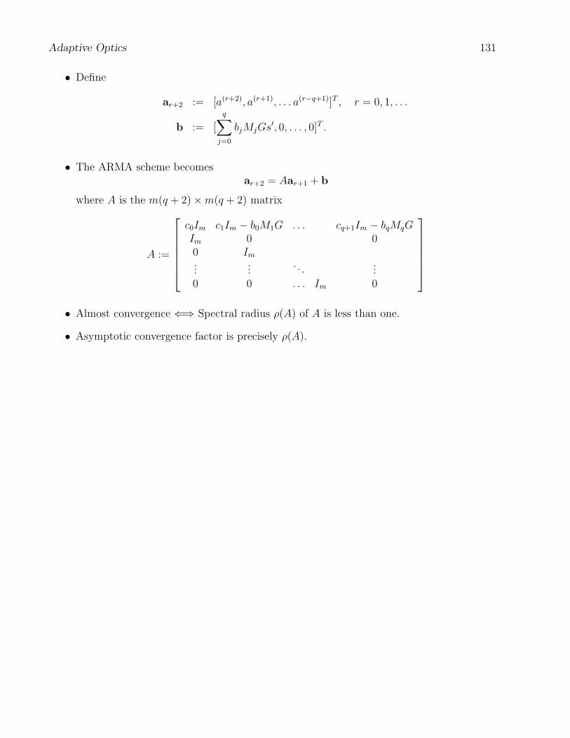
• Define

ar+2 := [a(r+2), a(r+1), . . . a(r−q+1)]T , r = 0, 1, . . .

b := [

q∑

j=0

bjMjGs′, 0, . . . , 0]T .

• The ARMA scheme becomesar+2 = Aar+1 + b

where A is the m(q + 2)×m(q + 2) matrix

A :=

c0Im c1Im − b0M1G . . . cq+1Im − bqMqG

Im 0 00 Im...

.... . .

...0 0 . . . Im 0

• Almost convergence ⇐⇒ Spectral radius ρ(A) of A is less than one.

• Asymptotic convergence factor is precisely ρ(A).

132 Estimation

Numerical Simulation

• Consider the 2-cycle delay scheme

a(t+ 2∆t) = a(t+∆t) + 0.6H†W †∆s(t).

• Test data:

surface positions n = 5number of actuators m = 4number of subapertures ` = 3size of random samples z = 2500H = rand(n,m)W = rand(`, n)G = WH

Lφ = rand(n, n)Lε = diag(rand(`, 1))µφ = zeros(n, 1)µε = zeros(`, 1)

• Random samples:

φ = µφ ∗ ones(1, z) + Lφ ∗ randn(n, z),

ε = µε ∗ ones(1, z) + Lε ∗ randn(`, z).