detailed economic analysis a. introduction

Henan Xichuan Integrated Ecological Protection and Environmental Improvement Project (RRP PRC- 53053-001)

DETAILED ECONOMIC ANALYSIS

A. INTRODUCTION 1. This appendix documents the economic analysis completed as part of the TrTA for the Henan Xichuan Integrated Ecological Protection and Environmental Improvement Project. The Project covers the county of Xichuan in the province of Henan. The Project is expected to revitalize the economy with improved water quality and sustainability of agricultural production systems in Xichuan county. The project has three components: (i) developed institutional capacity of Xichuan County Government (XCG), (ii) improved soil and water conservation practices, and (iii) implemented rural water services. B. MACROECONOMIC AND SECTOR CONTEXT 2. Henan is one of the poorest provinces in the People’s Republic of China (PRC) and Xichuan County in Henan Province is one of 65 national poverty counties with low human development index declared by the PRC Government. The Xichuan County has 724,600 population, of which 560,000 (77.3%) are farmers with average per capita income of CNY9,900, which is below the national average rural per capita income of CNY13,450. The annual population growth in the county is estimated at 4.6%, the highest among other counties in the province. Lying at the headstream of the middle line of the south-to-north water diversion project, the county however faces various restrictions on development mainly due to the fear of degrading water quality and quantity in the Danjiangkou Reservoir. Rocky desertification is a critical problem in this agrarian county with very low soil formation rate and high permeability of carbonate rocks leading to highly fragile and vulnerable environment that is susceptible to deforestation and soil erosion, exacerbated by unsustainable farming and uncoordinated development practices. Therefore, the government is in need of a unique approach for the rural vitalization that can secure the livelihood of the farmers and protect the environment. 3. Xichuan County of Nanyang Municipality is located at the junction of the southwest border of Henan Province, Hubei and Shanxi provinces. It also lies at the extension of the southeast margin of Qinling mountain. In this area, Danjiang River, which originates in Qinling of Shanxi Province, joins Hanjiang River of Hubei Province in the southwest of Xichuan. The Danjiang River is a major tributary of the Danjiangkou reservoir, which is the largest fresh lake in Asia. Xichuan County is famous because it is the headstream of the middle line of the South-to-North Water Transfer Project (SNWTP). The Xichuan County faces various restrictions on development mainly due to the fear of degrading water quality and quantity in the Danjiangkou Reservoir, a source of the SNWTP that serves 50 million people in 30 major cities in Northern PRC including Beijing and Tianjin. 4. The South-to-North Water Diversion Project delivers pure Danjiang water to the arid Beijing-Tianjin area. However, the resident of the town in Xichuan mainly relies on the extraction of deep groundwater as a major water supply source. The groundwater level continuously drops, affecting the surrounding environment. According to notice on Strengthening Urban Groundwater Water Supply Permit Management and Strictly Controlling Groundwater Exploitation Work (Yushui Zhengzi [2009] No. 7) and "Henan Provincial Water Resources Department Notice on Announcement of Groundwater Over-exploitation in Henan Province" (Yushui Zizheng [2014 [76] and other documents, residents are prohibited to use self-prepared wells, and reduce the exploitation of groundwater resources.

http://www.adb.org/Documents/RRPs/?id=53053-001-3

http://www.adb.org/Documents/RRPs/?id=53053-001-3

2

5. Flood damage seriously affects income levels and quality of life, especially in low income households, and uninsured urban settlements. The intangible impacts of flooding (anxiety, poor health) should also not to be overlooked. Furthermore, the county experience serious soil erosion due to lack of slope protection of river banks and steep slopes. Eroded sediment hindered the water carrying capacity of the rivers and lakes. The proposed river rehabilitation will considerably reduce expected flood damage. In conjunction with the wastewater subproject there will be a marked improvement in the river environment. 6. The sewage network currently covers 85% of urban area but almost no such facilities exist in rural areas in Xichuan County. There are 14 wastewater treatment plants (WWTPs) of capacity 100,300 tons/day but that serve only a fraction of total urban areas in the county despite the fact that total annual wastewater production in the county is only 13 million tons. Lack of public toilets in both business and tourist destinations, affected 200,000 locals and 500,000 tourists annually. The county produces 202,000 tons of solid waste (additional 1,000 tons of plastic waste) and 128,700 tons of farm waste annually but due to the lack of waste collection, transfer and treatment facilities, solid wastes are openly dumped on public spaces and ultimately discharged into the rivers. 7. Cold storage facilities are currently constraining the growth of the fruit tree production in Xichuan county. The 13th Five-Year Development Plan, the agricultural economic development rate of Xichuan is expected to increase by 15% and the total agricultural output value will reach CNY5.5 billion. The production base of fruits and agricultural products is the key focus of development plan, which will promote a continuous expansion of the fresh-keeping warehouse. Investment in reducing post-harvest losses through better handling of fruits and other agricultural products, adopting improved technologies and efficient marketing would lead to a reduction of the carbon footprint of food wastage. 8. Agricultural water conservation is high on the government’s agenda. Strong emphasis has also been placed on agriculture water saving and increase agricultural production and farm income. Irrigated agriculture is still the major water user in Xichuan. The project will introduce the use of smart irrigation where 50% of agriculture water would be saved and the agricultural yield per unit of water consumed would improve. C. ASSUMPTIONS AND PARAMETERS

9. The economic analysis was conducted in accordance with Asian Development Bank’s (ADB) Guidelines for the Economic Analysis of Projects (1997, 2017),1 and other good practices guides. The major assumptions of the analysis are as follows:

(i) Economic costs and benefits are valued based on constant August 2020 prices. converted to CNY using an exchange rate of CNY7.8562 per US$1.00 (as of 13 August 2020). (ii) Economic costs of capital works and annual operation and maintenance are calculated from project cost estimates; price contingencies, financial charges and taxes and duties are excluded in the analysis but includes physical contingencies of 5%. (iii) All costs were valued using the domestic price numeraire; traded outputs are adjusted to economic prices using a shadow exchange rate factor of 1.012 and non-traded outputs

1 ADB. 1997. Guidelines for the Economic Analysis of Projects, Manila; ADB. 2017. Guidelines for the Economic Analysis

of Projects, Manila. 2 Asian Development Bank estimates.

3

are valued at domestic market prices; skilled labor is adjusted to its economic value using an opportunity cost of scarce labor of 1.0 and unskilled to its economic value using shadow wage rate of 0.8;3 (iv) Analysis was conducted from 2021-2046, including 6 years of construction and 20 years of operation for improved urban and rural water supply system, integrated river management, kitchen waste and municipal sludge processing, improved rural sewage and wastewater management, and adoption of smart irrigation. (v) Residual asset values are treated as benefits at the end of the project life, if any; (vi) The economic viability of the project was determined by computing the economic internal rate of return (EIRR) and comparing it with the economic opportunity cost of capital of 9%; (vii) Economic value of land, as a part of land acquisition and resettlement costs, is based on its economic opportunity costs: that the income foregone due to resettlement, if any.

10. The economic viability of the project was determined by computing the economic internal rate of return (EIRR) and comparing it with the economic opportunity cost of capital of 9%. The viability of the project was tested through sensitivity analysis under scenarios in which key variables such as capital costs, O&M costs and benefits changed from those anticipated. Sensitivity indicators and switching values are calculated. Distribution of project benefits and poverty impact analyses were also undertaken to determine how much of the economic benefits resulting from the investments will directly benefit the poor. D. PROJECT SCOPE AND OUTPUTS

11. The detailed outputs and components are presented below.

Table 1. Project Scope and Outputs Output/Component Sub-project

Output 1 - Institutional capacity of Xichuan County Government

developed

1.1 Institutional Support

1.1.1 Institutional support for agricultural marketing reform

1.1.2 Provision of fruit cold storage facilities

1.2 Community-based Environmental Management

1.2.1 Awareness improvement

1.2.2 Pilot non-degradable waste including plastic separation tool

1.3 Institutional Capacity Building for Flood Mitigation

1.3.1 Installation of hydro-meteorological and water quality devices

1.3.2 Strengthening local early flood warning system

1.3.3 Enhancement of emergency response

1.4 Rural Eco-tourism

1.5 Soil Erosion Mitigation Measures

Output 2 - Soil and water conservation practices improved

2.1 Forestry and Fruit Farming Development

2.1.1 Smart irrigation system

2.2 River Training and Flood Risk Management

2.2.1 Integrated river management in Danjiang Henan-Hubei Section

2.2.2 Integrated river management in Xi River

3 The specific conversion factor for unskilled labor was sourced from the economic analysis associated with ADB Project

Number 52026-001 Anhui Huangshan Xin’an River Ecological Protection and Green Development Project. November 2019.

4

Output/Component Sub-project

2.2.3 Dongfeng canal reconstruction

2.3 Drainage Improvement and Waterlogging Alleviation

2.3.1 Improvement of drainage system and provision of waterlogging alleviation measures

Output 3 - Rural water services implemented

3.1 Rural Wastewater Management

3.2 Rural Solid Waste Management

3.2.1 Xichuan County food waste and municipal sludge treatment center

3.3 Water Supply for Urban and Rural Areas Source: Final Feasibility Study Report, August 2020

E. PROJECT OUTPUT AND LEAST COST OPTIONS 12. Least cost analysis has been conducted throughout component selection and preliminary design to ensure that the selected investments are the most economical interventions. The proposed investments are the least cost solutions to achieve the objectives of the project. The identification of feasible project alternatives that will have a better economic return were identified as part of the TrTA technical analysis report. Least-cost analysis was completed on the subcomponents to compare the cost effectiveness of the design options. Comparisons were based on net present values. The discount rate for all comparisons was 9%. 13. The subprojects will treat wastewater that is currently discharged into rivers and to protect the water source basin of the South-to-North Water Transfer Project. This will improve the water quality of the receiving water bodies, as well as the living environment of the residents and protect public health. To be able to achieve this all WWTPs will adopt treatment with ultra violet disinfection, discharging effluent meeting Class 1A standard which is the most stringent standard under the Discharge Standards of Pollutants for Town Sewage Treatment Plant. Because of this strict requirement, all WWTPs will adopt secondary treatment followed by tertiary treatment then disinfection. For secondary treatment, most WWTP will adopt the A2/O oxidation ditch process. This is a mature and dependable technology already adopted in China. The process entails that wastewater goes through anaerobic-anoxic-oxic (thus A2/O) treatment in the oxidation ditch (which is a modified activated sludge process) for effective removal of BOD, nitrogen and phosphorus. Each subproject will likely deploy a combination of these methods. 14. Materials selected include ductile iron pipe, pre-stressed concrete cylinder pipe (PCCP), and steel pipe, for pipes with diameters 1,000 meter. Construction methods include both horizontal directional drill [also called pipe jacking] and open cut. When pipes are to be installed 6.0 m below ground, underneath rivers, or going through obstacles, Pipe jacking will be applied. While open cut is a conventional method for pipeline installation, pipe jacking should be considered whenever the geotechnical and external conditions allow, since it causes less destruction to the road surface and less social, environmental and traffic impacts to the public. 15. On revetment’s ecological protection slope, different materials (mostly a combination of different materials) will be used in different subprojects taking into account protection strength, anti-erosion and anti-scour performance, vegetation coverage, landscaping and ecological effect, and construction cost. These materials include vegetation slope, Renault pad revetment and plant slope protection have comparatively better ecological effect than gabion revetment and vegetated concrete revetment. 16. Below are the results of the least-cost of the technical alternatives considered for wastewater distribution pipeline materials and slope protection materials.

5

Table 2. Results of Least Cost Analysis

NPV (CNY/M2) Least Cost Preferred in FSR Plant Slope Protection Capital Cost 23.9 O&M Cost 42.6 Total Cost 66.5 ✓ ✓

Ductile Iron Pipe (DN 1000) NPV (CNY/M) Capital Cost 12.7 O&M Cost 24.2 Total Cost 36.9 ✓ ✓

O&M = operation and maintenance, M = meter, M2 = square meter Source: Consultant’s estimates

F. ECONOMIC COSTS AND BENEFITS

17. Economic Costs. The project costs include capital costs of civil works, equipment, materials, land acquisition and resettlement, project management, capacity building, physical and price contingencies and financing charges during implementation. The overall project investment cost is US$463.3 (CNY3,176.8 million equivalent)4. The economic analysis of the individual subproject used the financial cost developed from the engineering cost estimates5. The economic cost of each individual subproject will be discussed in each subproject’s economic evaluation. The total estimated project investment cost is in Table 3 below.

Table 3. Total Project Investment Cost (in million)

Item CNY US$ A. Base Cost

1. Institutional capacity of XCG developed 278.9 40.7 2. Soil and water conservation practices improved 1,608.0 234.5 3. Rural water services improved 940.7 137.2

Subtotal (A) 2,827.6 412.4 B. Contingencies 291.9 42.6 C. Financial Charges during Implementation 57.4 8.4 Total Cost (A+B+C) 3,176.8 463.3

Source: Feasibility Study Report, TrTA Consultants Note: Figures may not precisely tally because of rounding.

18. Economic Benefits. The following economic benefits were considered in evaluating the economic viability of the proposed subprojects:

(i) For water supply services improvement, rural sewage and wastewater management and food waste and municipal sludge treatment center, the major economic benefits are assumed from (i) incremental benefits measured through willingness-to-pay (WTP) for water supply and wastewater; and (ii) non-incremental benefits valued at resource cost savings from water supply, rural wastewater and solid waste management improvements, (iii) improved public health with less productivity losses and reduced medical costs, and improvement of water quality.

(ii) For river improvement and flood risk management, the economic benefits are estimated from (i) savings from avoided damages due to reduction of flood risks with improvement in

4 Exchange rate CNY/US$ = 6.8562 (as of 13 August 2020). 5 Costs of components that were subjected to economic evaluation. Excludes price contingencies and financing costs.

6

river channels and embankments and (ii) benefits from reduced flood damage due to early flood warning system.

(iii) For smart irrigation, the economic benefits are irrigation benefits such as increased agricultural production from improved irrigation efficiency.

(iv) For fruit cold storage, the economic benefits are avoided post-harvest losses.

G. Overall PROJECT ECONOMIC INTERNAL RATE OF RETURN 19. The overall project is economically viable with an EIRR of 12.2% and NPV of CNY541.5 million (Table 4). The individual output EIRRs are 14.7% (Output 1), 12.3% (Output 2) and 12.6% (Output 3). Sensitivity analysis examined the impact of changes in costs, benefits, and implementation delay on economic performance. The estimated EIRRs for the overall project remain above 9% in all scenarios. The analysis suggests that the project economic performance is generally robust against identified risks. The project switching value for cost overrun is 34.5%, and 23.3% for a decrease in benefits. The detailed computation of the overall project EIRR and individual output EIRR can be found in Annex B while the summary overall project EIRR and individual outputs EIRR are shown in Table 4 through Table 7.

Table 4. Overall Project EIRR and Sensitivity Analysis

Sensitivity Test EIRR NPV

(CNY M) SI SV (%)

Base Case 12.2% 541.5 Increase in capital cost by 10% 11.3% 408.3 0.8 34.5 Increase in operating costs by 10% 11.9% 482.7 0.3 98.1 Decrease in benefits by 10% 10.8% 295.4 1.1 23.3 All of the above 9.6% 103.4 2.1 12.3 One-year lag in implementation 11.9% 439.8 0.2

EIRR = economic internal rate of return, NPV = net present value, SI = sensitivity indicator, SV= switching values

Table 5. Output 1: Institutional Capacity of XCG Developed (Fruit Cold Storage)

EIRR and Sensitivity Analysis


(CNY M) SI SV (%)



Table 6. Output 2: Soil and Water Conservation Practices Improved

EIRR and Sensitivity Analysis


(CNY M) SI SV (%)



7

Table 7. Output 3: Rural Water Services Implemented EIRR and Sensitivity Analysis


(CNY M) SI SV (%)



20. Distribution of Economic Benefits. The economic analysis of the project also assessed the distribution of benefits for various beneficiaries. farmers, workers, municipal and provincial governments, industries, and communities (direct recipients of improved wastewater and water supply services) are expected to benefit from the project. The community will receive the largest share, accounting for 61% of the total benefits. The distributional analysis estimating the project's economic net present value yields a poverty impact ratio of 0.20, i.e., the poor are expected to receive 20% or CNY128.9 million of project benefits. The results of the social survey show that 15% of the rural population in the project areas is living below the poverty line.

Table 8. Distribution of Benefits and Poverty Impact Analysis

Item FIN

ECON PV*

Econ-Fin PV

Government Community Labor Farmers Total PV*

Benefits:

Benefits Reduced flood damages 498 622 124 124 124

Improved WS services 612 765 153 153 153

Improved WW services 292 365 73 73 73

Reduced health risks 108 135 27 27 27

Increased agricultural production 241 301 60 60 60

Reduced post-harvest losses 142 177 35 35 35

Improved Drainage 77 96 19 19 19

Total benefits 1,969 2,461 492 0 397 0 96 492 Costs Capital 1,422 1,408 -14 -14 -14

O&M 537 511 -26 -26 -26

Taxes and duties 109.7 0 -109.7

-109.7

-109.7

Unskilled labor 62.2 49.3 -12.9 -12.9 -12.9 Total costs 2,131 1,969 -162 -149 0 -12.9 0.0 -162

Net benefits -162 492 654 149 397 3.0 96 654 Net benefits to the poor 29.9 79.3 0.6 19.1 128.9 Poverty impact ratio 0.20

*PV at 9%

8

BENEFITS OF SMART IRRIGATION SUB-PROJECT 21. The proposed subproject will be implemented in a 38,537 mu of fruit tree plantation in 10 townships. It will cover 8 fruit trees, namely, cherry, pear, kiwi, pomegranate, apricot plum, peach, persimmon, and grapes. Table 9 shows the location of the plan irrigation area and Table 10 shows plan irrigation area with the corresponding fruit trees.

Table 9. Plan Irrigation Area No. Township Area (mu)

1 Zijingguan 2,600 2 Maotang 4,350 3 Jinhe 5,900 4 Jiuchong 7,954 5 Siwan 1,800 6 Houpo 6,193 7 Xihuang 1,490 8 Xianghua 700 9 Madeng 3,300

10 Shangji 4,250 Total 38,537

Source: Feasibility Study Report, July 2020

Table 10. Plan Irrigation Area Fruit Tree

No. Fruit Tree Area (mu)

1 Persimmon 1,028 2 Apricot-plum 5,540 3 Peach 4,110 4 Soft Seeds Pomegranate 9,725 5 Kiwi Fruit 1,600 6 Pear 8,104 7 Cherry 8,080 8 Grape 350

Total 38,537 Source: Feasibility Study Report, July 2020

22. Irrigation is essential for most agricultural production and agricultural water use accounts for a significant proportion of total water consumption. Droughts are expected to occur more frequently and this would lead to an increase in the demand for irrigation in many crops, including permanent crops. Smart irrigation, unlike traditional irrigation operate on a preset programmed schedule and timers, smart irrigation controllers monitor weather, soil conditions, evaporation and plant water use to automatically adjust the watering schedule to actual conditions of the site. One of the greatest advantages of a smart irrigation system is its ability to save water. The traditional watering methods can waste as much as 50% of water used due to inefficiencies in irrigation, evaporation and overwatering. Smart irrigation systems use sensors for real-time or historical data to inform watering routines and modify watering schedules to improve efficiency. 23. Economic Value of the Incremental Increase in Fruit Production. This was determined based on the increased crop production from without project to with-project situations. Four crops were considered: cherry, pear, pomegranate, and apricot covering about 81% of the plan area. The economic value was computed by multiplying the following factors: area of land used in planting (in mu); average yield (in kg/mu); and farm gate price of crop (in CNY/kg). Crop production cost is deducted from the gross production value to derive the net benefit. Incremental benefit is then

9

calculated by deducting the without project situation from the with-project situation. The crop budgets employed in the analysis are shown below.

Table 11. Crop Budget CNY/mu Big Cherry Pomegranate Apricot Plum Pear

Yield/kg 90 280 200 370 Inputs Seedlings 150 300 180 200 Fertilizer (organic) 900 900 900 900 Pest control 200 200 200 200 Water & Electricity 300 300 300 300 Labor 800 800 800 800 Total inputs (mu/kg) 29 14 34 6

Source: Xichuan County Project Management Office

24. Other benefits that were not quantified and valued in the analysis include improved health and nutrition of the project beneficiaries, increased water availability for agricultural activities, and more efficient management and monitoring of water resources. 25. Benefit-cost analysis. The main quantifiable benefit of the subproject is the net incremental value of production. Annual cost stream is determined to calculate the economic returns of the subproject. Costs are similarly projected with investment costs falling in the first six years followed by annual maintenance expenditure in each subsequent year. The calculated economic internal rate of return is 11.5% and net present value of the investment is CNY65.2 million (when applying a discount rate of 9%). Table below shows the summary results of the base case and sensitivity tests while the detailed computation is in Annex B.

Table 12. EIRR and Sensitivity Analysis


(CNY M) SI SV (%)



10

BENEFITS OF FRUIT COLD STORAGE SUB-PROJECT 26. Cold storage is keeping the product under the conditions that will enable the preservation of its quality for future marketing or processing to gain higher revenues. Cold storage for fruit tree crops as proposed in Xichuan can now be stored for longer periods, quality losses due to storage is decreased, commercial revenue from stored goods is higher and it is possible to find fresh fruits and vegetables in all seasons. The cold storage business also creates new employment opportunities in many sectors such as packaging and transportation. 27. There are significant losses in fruit tree crops produced globally during and after harvesting. The ratio of these losses varies between 5%-10% in developed countries and between 20%-40% in developing countries6. 28. The existing capacity of fruit cold storage in Xichuan county has reached more than 5 million tons, of which the storage capacity of fruit crop products in commercial system has reached more than 1.3 million tons, of which more than 700 thousand tons are mechanical cold storage and 600 thousand tons are ordinary storage. 29. At present, commercial treatment rate nearly reach 100% for post-harvest fruit in developed countries, while that of China and Henan Province is less than 1% of the total output. The amount of fruit stored in developed countries is about 45%-70% of the total fruit output, of which 30%-45% of the fruit is frozen in the form of low temperature preservation storehouse, while the amount of fruit stored in China is only 33% of the total output, and the low temperature frozen storage is only about 2% of the total storage. 30. Storage infrastructure of agricultural commodities in Xichuan is insufficient and/or inadequate, lacking the necessary equipment to maintain the uniformity of quality. This reduces the ability for distribution to where demand is high at the national level. Furthermore, the use of traditional storage structures has contributed to high levels of losses. At present, the total area planted to fruit tree crops in Xichuan County is about 160,000 mu. During the full harvest season, the total output of fruit tree crops reached more than 320,000 tons. Every year in China, about 25% of the agricultural products cannot be consumed due to decay, and some perishable fruits suffer losses of more than 30%. 31. This section covers the economic analysis of the proposed fruit cold storage facilities. The subproject consists of construction of 53 fresh fruit cold storage in 10 townships namely: Jingziguan, Maotang, Jinhe, Siwan, Jiuchong, Houpo, Xihuang, Xianghua, Madeng and Shangji in Xichuan County. The proposed cold storage is equipped with modern support facilities including electric power, refrigeration and auxiliary facilities. The implementation of the project will also strengthen existing transport industry and rural network sales and e-commerce logistics. The total design storage capacity is estimated at 20,300 tons. Table below presents the capacity and number of the proposed fruit cold storage.

6 Kader, A.A. 2002. Post-harvest Technology: An Overview in Post-harvest Technology of Horticultural Crops. University

of California. Agricultural and Natural Resources Publication No. 3311. USA.

11

Table 13. Capacity and Number of Fruit Cold Storage Town Number of Storage Capacity (ton) Output (ton)

Houpo 12 3,300 10,590 Jiuchong 6 11,600 39,674 Madeng 4 400 2,925 Xianghua 2 600 1,672 Shangji 12 1,900 10,880 Jinhe 5 600 6,550 Maotang 5 900 5,040 Xihuang 3 500 3,400 Siwan 3 400 4,700 Jingziguan 1 100 1,200 Total 53 20,300 86,631

Source: Feasibility Study Report, TrTA SD1b Technical Assessment Fruit Cold Storage. July 2020

32. Economic Costs. Capital costs were provided in the feasibility study report. Capital costs are distributed over the implementation period based on the implementation plan. The fruit preservation storage economic cost estimated at CNY74.3 million. O&M costs following project construction is estimated at 20% of the total subproject investment cost.

33. Economic Benefits. The economic benefits accounted for are those derived from losses that would be averted from constructing and/or expanding storage capacity. Unquantified benefits include increased in farmers income through off-season sales that increases the market price of the products. The availability and improvements of fruit cold storage infrastructure and the provision of capacity building will, on the other hand, reduce losses in Xichuan, which are currently estimated at 10 percent pre-harvest and 24 percent post-harvest. The project will make energy efficient and renewable energy technologies, particularly solar energy, available to the new cold storage infrastructure. For the economic analysis, subproject losses are estimated as the value of the fruit commodities at the production stage during which it was wasted. The estimated loss in terms of economic value is estimated at CNY32.5million7 (at post-harvest stage of the produce at an average 2020 constant price of CNY4.6 per kilogram). 34. There are other economic benefits that would be expected to accrue as a result of the proposed project, but as they are not easily quantifiable, they were not accounted for in the cost-benefit analysis. The economic benefits unaccounted for in the cost-benefit analysis include: (i) increased expected net revenues to fruit producers due to greater access to markets through improved fruit storage, and better access to market information for decision making; (ii) increased economic efficiency achieved through the systematization of market information; and (iii) local economic growth resulting from increased demand for local goods and services during construction and the operation of storage facilities. Further the project will contribute to improving food security through reduction of post-harvest losses. 35. Economic Internal Rate of Return. The results indicated that the proposed subproject is economically viable with an EIRR of 14.7% which exceeded the EIRR threshold of 9%. Sensitivity analysis examined the impact of changes in costs, benefits, and implementation delay on economic performance. The estimated EIRR for the project remains above 9% in all scenarios. The analysis suggests that the project economic performance is generally robust against identified risks.

7 Post-harvest losses estimated at 9% (average rate calibrated for South and Eastern Asian countries) based from FAO

food loss index of 13.8% recorded at different stages of the supply chain - production, post- harvest and processing.

12

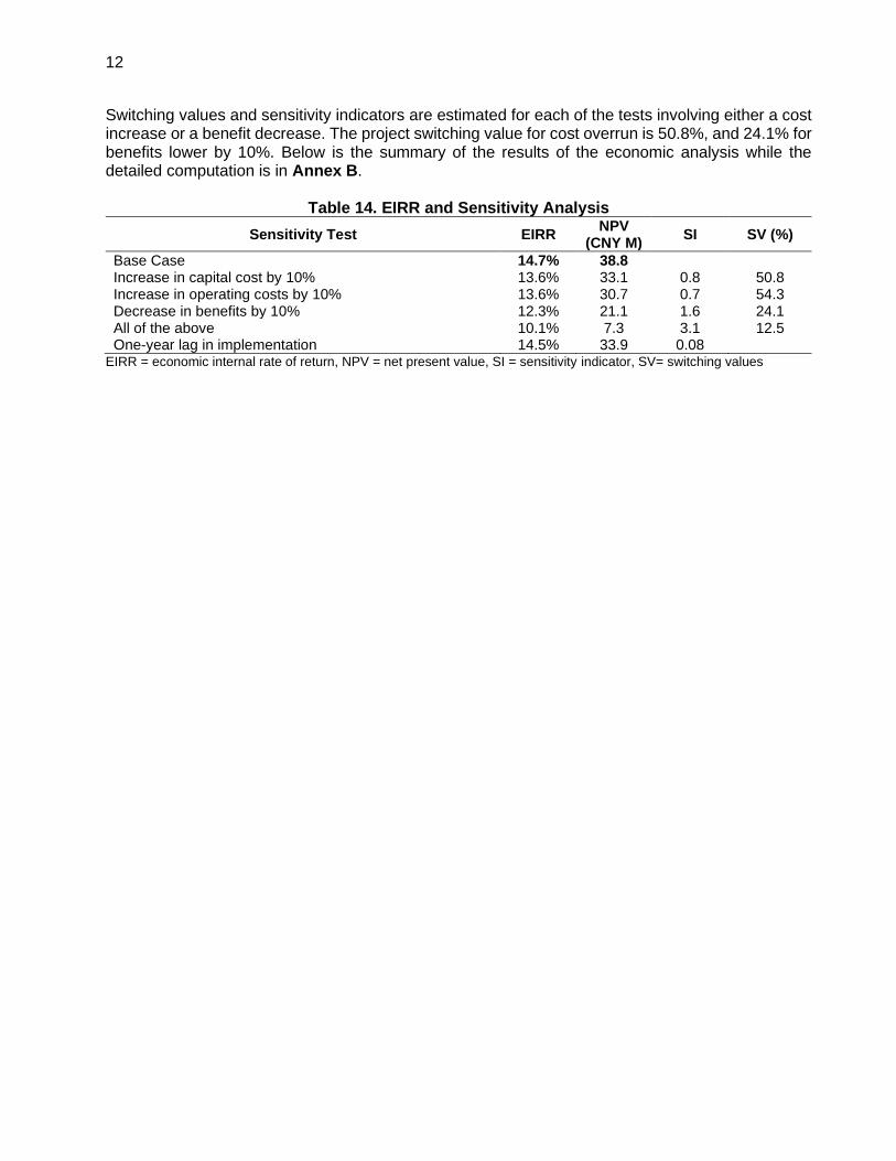
Switching values and sensitivity indicators are estimated for each of the tests involving either a cost increase or a benefit decrease. The project switching value for cost overrun is 50.8%, and 24.1% for benefits lower by 10%. Below is the summary of the results of the economic analysis while the detailed computation is in Annex B.



(CNY M) SI SV (%)



13

BENEFITS OF RIVER IMPROVEMENT AND FLOOD RISK MANAGEMENT SUB-PROJECTS 36. This section covers the economic analysis of (i) integrated river management in Danjiang Hubei-Henan section and (ii) river management in Xi River. 37. During the flood in 2010, around 10,716 buildings in Xichuan were destroyed and the flooded farm land was nearly 3,920 hectares. Although after many years of integrated management, the flood control capacity of Danjiang River has been increased, there are still problems such as short embankment and severe erosion damage that let the frequent flood continue to threaten the safety of local residents. Moreover, as results of the floods of Danjiang River, most of the buildings located closed to the river are dilapidated. The existing flood control measures of Danjiang River can merely defense 2 to 5-year flood return period. 38. While the Xi River, is mountainous river but its downstream is relatively flat and passes through the southern part of the city center. The flood protection level of the Xi River embankment varies. Most of river embankments cannot meet the flood protection standards of the current "Master Plan" of Xichuan County. Garbage piled up in many places along the river which seriously affects the water environment of the river, especially during floods where garbage is washed down to the river causing blockage of the river. Houses and buildings adjacent to the river do not have flood protection from river overflows. There is no sewage collection and discharge system in the area and hence, sewage is directly discharged into the river. 39. The subprojects will provide protection against floods up to a 20-year return period. The detailed works for the river improvement is shown below.

Table 15. Scope of Subprojects No. Subproject Activity Description

1 Integrated River Management in Danjiang Henan-Hubei Section

Embankment

New reinforced embankment of 18.765 km, of which newly-built retaining wall embankment of 6.347 km, newly-built sloping wall embankment of 6.971 km, and reinforced embankment of 5.447 km

Culvert and Sluice Construct 10 new culvert and sluice, rebuild 1 culvert and sluice

River Flood Control Information Program

Purchase of water level acquisition equipment, and online surveillance device

2 Improvement of Xi River River Training

Renovate the Xi River, and Shiban River, with a total length 10.39 km, which includes river dredging, bank slope regulation, dike and flood control road construction; construct 1 new ecological weir, and 3 culverts; demolish and rebuild 1 ecological water storage weir, and 2 submersible bridges; demolish 2 abandoned submersible bridges; reconstruct 2 connecting gates

Source: Feasibility Study Report, SD04 and SD03a TrTA Technical Assessment Report, July 2020

40. Costs. Capital costs were provided in the feasibility study report. Capital costs are distributed over the implementation period based on the implementation plan. The river integrated management improvements economic cost estimated at CNY365.8 million and CNY81.2 million for Danjiang River and Xi River, respectively. O&M costs following project construction is estimated to be about 5% of the total subproject investment cost if no O&M costs are provided in the FSR.

14

41. Benefits. There are three estimation methods in the current literature for evaluating flood risk reduction benefits: (i) property damage avoided (PDA), (ii) hedonic pricing, and (iii) contingent valuation (CV) methods. PDA method calculates the benefits repair costs to a specific property in the affected area with and without a flood risk reduction project for a given flood event. PDA is an indirect benefit measure since repair costs are a proxy of flood reduction as a commodity. Hedonic pricing method estimates the implicit price real estate market traders are willing to pay for an incremental reduction in the level of flood risk. Hedonic pricing method is also an indirect measure, and it is based on revealed preference instead of hypothetical measures such as PDA. CV method is a direct hypothetical approach to benefit estimation since it asks households for their willingness-to-pay (WTP) for a prospective change in a non-market resource8. 42. Comparing the three methods, the literature reports that hedonic methods generated the largest estimates for the most flood prone areas. For those with over 2% flood risk, the hedonic pricing estimates are 2 to 3 times greater than PDA and CVM. Therefore, hedonic method indicates that people are willing to pay a substantial premium for reductions in flood risk. Since a thorough and detailed survey was not conducted to estimate the WTP, CV method cannot be used in the current analysis. Based on the afore-cited discussion of the estimation methods, the PDA method is used to estimate the economic benefits for the proposed component because it is the most conservative approach. The benefits of flood prevention are then calculated by PDA method, which will evaluate the losses of a flood under current economic situation, according to the estimated losses during past years. Flood losses were based on previous years provided by the county government. 43. Estimates of damages from flood focused mainly on direct damages due to difficulties in accounting for indirect and non-monetary damages. The analysis relied on the use of information on past damages to assess the impact of floods in the project area. Consequently, past damages were applied as a basis for coming up for the current potential damages. Damage data were updated to account for inflation and growth of assets due to urban development (apply an index of real growth in fixed assets). Historical flood damage data were available for 5 flood event years starting in 2000 for Danjiang River and 3 flood event years starting 1999 for Xi River. These data were adjusted to 2020 values using an inflation factor as well as an index of real growth in fixed assets. 44. Event Damage Valuation. In the without project situation Xichuan experiences substantial damage due to frequent flooding cause by severe siltation and poor flood-discharge capability of the Danjiang and Xi Rivers. The damage mainly affects private properties along the flooded rivers. Record of flood obtained from the County Government PMO submitted flood events for Danjiang River and Xi River are presented in the table below.

Table 16. Historic flood damage, (CNY million) River 1999 2000 2002 2007 2010 2011 2017 2018

Danjiang River 103.9 37.2 74.1 576.0 42.6 Xi River 1.0 32.0 5.0

Source: Project Management Office, Xichuan County

45. Estimates of damages from flood focused mainly on direct damages due to difficulties in accounting for indirect and non-monetary damages. The analysis relied on the use of information on past damages to assess the impact of floods in the project area. For the without project situation, the

8 ADB. December 2006. Gunatilake, et al. Economic Research and Regional Cooperation Department (ERCD) Technical

Note Series No.19. Willingness-to-Pay and Design of Water Supply and Sanitation Projects: A Case Study.

15

annualized value of damage due to flooding was assumed to increase following the growth trend of rapid urban and industrial development that is expected to occur. Consequently, past damages were applied as a basis for coming up for the current potential damages. Damage data were updated to account for inflation using CPI as an appropriate indicator of overall inflation and growth of assets due to urban development (apply an index of real growth in fixed assets). Historical flood damage data available were adjusted to 2020 values using an inflation factor for fixed assets as well as an index of real growth in fixed assets9. This was achieved by adjusting the estimated value of damage by the average annual real growth rate of urban and industrial development that has occurred in Xichuan over the past 3 years, an annual average of 4%. The adjusted damage values for each river are shown below.

Table 17. Adjusted Damage Cost

1999-

2020

2000-

2020

2002-

2020

2007-

2020

2010-

2020

2011-

2020

2017-

2020

2018-

2020

Danjiang River

-

1,022.4

470.5

299.3

1,105.4

74.9

-

-

Xi River

32.9 -

-

-

63.9

-

6.0

-

Source: Consultant estimates

46. Total damage estimates. The figure below shows reference and project case event damage plotted against probability. Purely illustratively it shows damage in the reference (without project) case starting at a return period (T) of 5 years (equivalent to an annual exceedance probability of 0.2). The project gives protection from T=20 years (probability of 0.05). The annual average (expected) benefit of the intervention is shaded gray. In this section estimates of the total (reference case) damage are presented, i.e. the PV of the annual damage represented by the total shaded area in the figure.

Figure 1: Flood Defense Benefits

47. The annualized value of flood damage was estimated for floods with a return period between 5 and 10 years, and between 10 and 20 years, based on the probability of these events as 20%, 10%,

9 Source of data: Henan Statistical Yearbook, 2017. The GDP deflator was used for the inflation factor.

0

50

100

150

200

250

300

0.500.200.100.050.020.01

Even

t da

mag

e in

CN

Ym

Probability/frequency per year (log scale)

Reference case(without project)

Project case

`

16

and 5% respectively. For floods with a return period of more than 20-years no estimate of annualized value was attempted since the with- and without-project situations are expected to be similar. Flood protection measures through dredging, embankments, channel improvements, and management provided by the Project are designed to protect up to 20-year flood. The flood return frequency of a 20-year flood is 5%. Protection to a 20-year flood means that the 20-year flood will not cause any damage. 48. The financial value of vulnerable assets was conservatively assumed not to increase during the forecast period. Expected annual damages estimated at CNY94.6 million and CNY16.8 million for the Danjiang River and Xi River, respectively. The financial values of flood damages were converted to their economic values which was estimated based on the assumption that the damages could be divided into 30% foreign exchange, 60% local currency and 10% unskilled labor and then applying the appropriate conversion factors to each part. The economic values are estimated at CNY93.0 million and CNY16.5 million for Danjiang and Xi River, respectively. The value of the vulnerable assets was conservatively assumed not to increase in real terms over the forecast period. The estimated values of flood damage for specific floods and annualized values for flood intervals are shown in the Table below.

Table 18. Estimated Flood Damage and Annualized Values

Item

Estimated value of damage from flood of specified

probability (CNY million) Annualized value of damage for floods within frequency

ranges (CNY million)

Annualized economic value of flood damage up to 20-year (CNY

million)

Return Period

5-year 10-year 20-year 5-10 year 10-20 year

Xi River 12.8 3.3 0.3 13.4 3.4 16.5

Danjiang River 15.0 77.0 15.0 15.8 78.9 93.8

Source: Consultant’s estimates

49. Flood Damage Reduction with Flood Warning10. The estimated savings from flood warnings was based on Day’s methods, it was assumed that a 3-hour was feasible in the project areas. This amount of warning results in a 5% reduction in expected damages. Actual savings are assumed to be half this amount or an annual savings of CNY2.4 million.

Figure 2: Flood Damage Reduction from Flood Warning

10 Kim M Carsell, Nathan D. Pingel and David T. Ford. Quantifying the Benefit of a Flood Warning System. Natural Hazard

Review, Volume 5, Number 3, August 1, 2004.

y = 0.8463x - 0.1222

-10

0

10

20

30

40

50

0 10 20 30 40 50 60

Dam

age

Red

uct

ion

wit

h

War

nin

g-%

Hours of Flood Warning

17

50. EIRR Danjiang Integrated River Management Improvement. Net present value (NPV) and economic internal rate of return (EIRR) was calculated for the subproject using the methods and parameters discussed above. The results indicated that the proposed subproject is economically viable with an EIRR of 13.2% which exceeded the EIRR threshold of 9%. Sensitivity analysis examined the impact of changes in costs, benefits, and implementation delay on economic performance. The estimated EIRR for the subproject remains above 9% in all scenarios. The analysis suggests that the subproject economic performance is generally robust against identified risks. The switching values analysis indicates that to maintain component EIRR at 9%, benefits should decline by not more than 28.6% while costs should not increase by more than 39.7%. A simultaneous decrease in benefits and increase in costs should not be more than 15.2%. Below is the summary of the results of the economic analysis for the Danjiang integrated river improvement while the EIRR detailed computation is in Annex B.



(CNY M) SI SV (%)



51. EIRR Xi River Improvement. The EIRR for the Xi River is 11.7% as set out in Table 18. The EIRR of the subproject exceeds the economic opportunity cost of capital of 9% and is therefore accepted. The NPV at 9% is CNY18.1 million. An analysis to test the sensitivity of the EIRR to adverse changes in key variables was undertaken. The subproject is most sensitive to a simultaneous increase in costs and decrease in benefits result in the EIRR declining to 8.9%. Below is the summary of the results of the economic analysis for Xi river improvement while the detailed computation is in Annex B.



(CNY M) SI SV (%)

Base Case 11.7% 18.1 Increase in capital cost by 10% 10.6% 11.9 0.9 26.1 Increase in operating costs by 10% 11.4% 15.9 0.3 86.0 Decrease in benefits by 10% 10.2% 7.8 1.2 18.3 All of the above 8.9% (0.7) 2.4 9.7 One-year lag in implementation 11.5% 15.2 0.1


18

BENEFITS OF RURAL WASTEWATER MANAGEMENT SUB-PROJECT 52. Due to poor infrastructure and inadequate environmental management, untreated wastewater has been discharging directly into rivers and streams. Management of wastewater has been identified as a key thrust area under the 13th FYP for Water Pollution Prevention and Soil Conservation in Danjiangkou Reservoir Area and Upstream sets a goal for urban wastewater treatment of 80% of wastewater generated. WWTPs will be designed to produce an effluent meeting the current Class 1A discharge standards. The main pollutants are COD, ammonia nitrogen and SS, as well as a large amount of sulfur dioxide, smoke and dust. The amount of COD and ammonium nitrogen being discharged has exceeded the environmental limits set by the government, causing serious negative impact on the quality of water resources. 53. Xichuan County is the water source of the South-to-North Water Transfer Project. The implementation of the said project has increased the need for ecological and environment protection in Xichuan County. Due to insufficient investment in ecological construction and pollution control, the rivers and wetlands have been polluted, the point source pollution caused by direct discharge of domestic sewage, and non-point source pollution caused by surrounding agricultural activities, not only threatening the water quality of source of the South-North Water Transfer project, but also increased the pollution load of the Danjiang and Danjiangkou reservoirs. 54. The objectives of the subproject is to increase the collection and treatment rate of rural domestic sewage through the construction of rural sewage pipes and treatment facilities, reduce pollution, improve the rural living environment, and improve the quality of life of rural residents, while protecting and improving the ecological environment of the water source basin of the South-to-North Water Transfer Project. 55. The subproject involves the construction of 14 wastewater treatment facilities and 2 sewage pumps for 23 villages in the towns of Shangji, Jinhe, Xianghua, Jiuzhong and Houpo and installation of 234.8 km of wastewater collection pipelines. Further, a 31.5 km of sewage pipelines will be installed in the industrial park to collect wastewater from the existing No.2 sewage treatment plant. The proposed wastewater treatment facilities will have an estimated daily capacity of 3,799 cubic meters (m3). 56. Economic benefit was measured through willingness-to-pay. Household willingness to pay (WTP) for wastewater collection and treatment was estimated for domestic consumers through contingent valuation approach. The payment method used is in the form of increments to current bills or new bills. The regression results are generally consistent with theoretical expectations on the relationship between the dependent variable, the mean WTP, and each of the independent variables. Valid responses (i.e., with significant coefficients) were tested for the variables on the bid, such as income and access to a septic tank. Households with higher income have a positive correlation with WTP for improved services. 57. Under the willingness to pay valuation method of estimating economic benefits, the average WTP is deemed to reflect the economic value of the improved services to the beneficiaries including health benefits. It is therefore a composite of monetary benefits from, for example, any savings from investing and maintaining an individual septic tank, health benefits and other non-monetary benefits such as an improved physical environment free from foul-smelling surroundings and vector-carrying insects, better living conditions and the like.

19

58. Validity test. The regression results11 are generally consistent with theoretical expectations on the relationship between the dependent variable, the mean WTP, and each of the independent variables. The output results converged after thirteen iterations which make this probit regression model an estimation method that can be used with some success.

Table 21. Validity Test

Model Unstandardized B Coefficients Std

Error Standardized

Coefficients Beta t Sig

Constant .850 .484 1.757 .080

Income (per year)

-1.777E-6 .000 -.097 -1.522 .129

Education (number of years)

.009 .009 .064 1.005 .316

Gender -.028 .077 -.023 -.359 .720

Age .006 .003 .111 1.754 0.81

Ethnicity -.793 .417 -.120 -1.902 .058

a. Dependent Variable: Bid (CNY/m3) Note: In determining the implied relationship between the dependent variable, mean WTP, and each of the independent variables, the decision rule adopted in this case is that whenever /t*/ > 2, the variable is significant (at 5% level of significance). 59. Valid responses were tested for the variables on the bids, income, age, type of dwelling and access to a septic tank. However, the tests show that education, gender, connection to the sewerage system and performance of existing services are insignificant, although the expected relationships were validated; the purpose of including these variables was to explore their possible effect on mean WTP, thus, the conclusion on whether or not they are significant cannot be rejected outright. 60. Regression results. Table 22 shows the probit regression results. In computing for the mean WTP, the following regression outputs were used with the bid as the independent variable. The mean WTP for wastewater12 of CNY1.72 per cubic meter (m3) was estimated by dividing the coefficient of the bid (-0.646) by the cumulative constant (1.113), that is, the sum of the products of the coefficients and the independent variables, and multiplying by negative 1. The computed mean WTP of CNY 1.72 per cubic meter (m3) was then applied to estimate the economic benefits.

Table 22. Regression Results for Estimation of Mean WTP

Parameter Estimate Std. Error Z Sig

95% Confidence Interval

Lower Bound

Upper Bound

Probita Bid values -.646 .101 -6.393 .000 -.845 -.448

Intercept 1.113 .286 3.889 .000 .827 1.399

a. PROBIT model: Probit(p) = Intercept + BX

61. WTP for Improved Water Quality. The quality of water in a receiving watercourse has no market price; it is a non-marketed good. Without public sector intervention, river water quality would be below standards. The market would fail to provide the quality that people want because they have no opportunity to express their preferences (except of course when buying property). In order to assess whether public sector intervention is worthwhile, a “contingent” market is devised. In the absence of any survey for improved water quality, a benefit transfer approach was employed. Table

11 Used SPSS statistical package, ver.20 12 Mean WTP = (- 646/ 1.113) * (-1) = CNY1.72 per m3

20

23 sets out comparable WTP values from various sources. Given that the project is intended to protect headwaters a relatively high value of CNY17.0 per month is taken. 62. Benefit transfer. The estimates of economic benefits for water quality improvement in Xichuan is based on results of contingent valuation (CV) survey conducted in Anhui Huainan and applied to Xichuan using specific-area socio-economic data. The estimated benefit function of Xichuan used the coefficients of Huainan benefit function. This approach requires data collection on those variables that were considered in Huainan site which affect the water quality benefits. Available secondary data on the mean values of the variables used in the analysis of the Huainan site are used to get the mean willingness to pay for the Xichuan site. The estimated mean willingness to pay for improvement on water quality in Huainan is CNY17.0 per household per month while the mean willingness to pay for Xichuan is calculated at CNY17.96 per household per month.

Table 23. WTP Value for Improved Water Quality

Source Location Date WTP per

Household per month

Characteristic Valued

PPTA 7607 a Hubei Huangshi 2011 CNY 24 Lake Rehabilitation PPTA 8151 b Hubei Huanggang 2013 CNY 12 Lake Rehabilitation

PPTA 8045 c Anhui Huianan 2013 CNY17 Improved Wastewater Collection, Watercourse Rehabilitation

Source: PPTA Consultants a Hubei Huangshi Urban Pollution Control and Environmental Management, PPTA economics appendix, 2011 b Hubei Huanggang Integrated Urban Environment Improvement Project, PPTA economics appendix, 2014 c Anhui Huianan Urban Water Systems Integrated Rehabilitation Project, PPTA economics appendix, 2013

63. Benefit-cost analysis. The economic rate of return were estimated using (a) an economic investment cost of CNY200.7 million, that is, after adjusting the financial investment cost to consider shadow prices for foreign exchange and labor, and deducting taxes and duties, (b) operation and maintenance costs, (c) a benefit stream based on a total of 1.4 million cubic meter (m3) per year of wastewater treated in 2027, the computed mean WTP of CNY1.72 per m3 was then applied to estimate the economic benefits. The WTP was adjusted for each year to reflect the expected growth in real income – by 5% per year to 2031, 3% per year to 2036, and 2% per year, thereafter, (d) a benefit stream based on CNY17.96 per household per month applied to the total beneficiary households to estimate the benefits from improved water quality. The economic rate of return for this sub-project component is estimated at 13.1%, above the ADB threshold of 9%. The subproject is most sensitive to a simultaneous increase in costs and decrease in benefits result in the EIRR declining to 10.5%. Below is the summary of the results of the economic analysis while the detailed computation is shown in Annex B.



(CNY M) SI SV (%)



21

BENEFITS OF FOOD WASTE AND MUNICIPAL SLUDGE TREATMENT SUB-PROJECT 64. The subproject will entail construction of a food waste and sludge treatment center with an estimated capacity of 100 tons per day broken down as follows: capacity of 70 tons per day of food waste and capacity of 30 tons per day of municipal sludge.

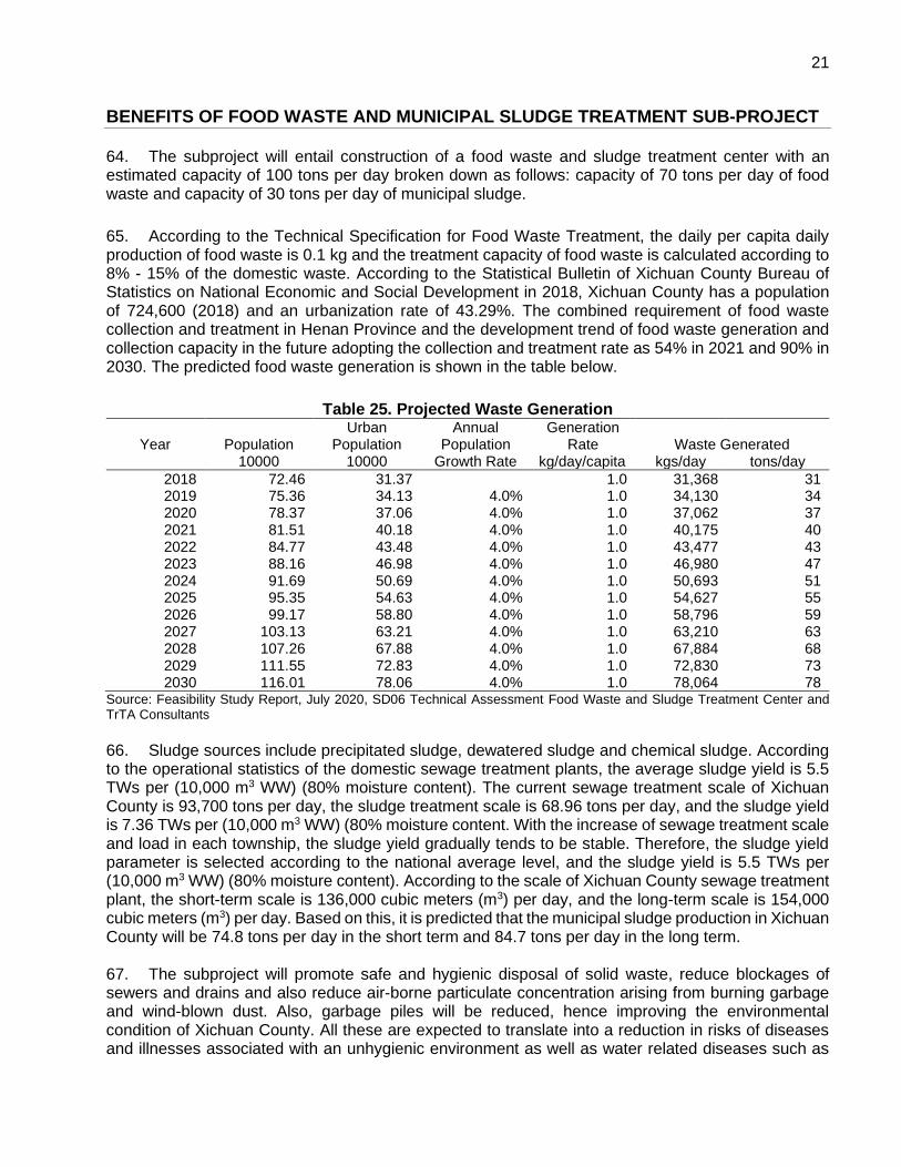
65. According to the Technical Specification for Food Waste Treatment, the daily per capita daily production of food waste is 0.1 kg and the treatment capacity of food waste is calculated according to 8% - 15% of the domestic waste. According to the Statistical Bulletin of Xichuan County Bureau of Statistics on National Economic and Social Development in 2018, Xichuan County has a population of 724,600 (2018) and an urbanization rate of 43.29%. The combined requirement of food waste collection and treatment in Henan Province and the development trend of food waste generation and collection capacity in the future adopting the collection and treatment rate as 54% in 2021 and 90% in 2030. The predicted food waste generation is shown in the table below.

Table 25. Projected Waste Generation

Urban Annual Generation Year Population Population Population Rate Waste Generated

10000 10000 Growth Rate kg/day/capita kgs/day tons/day

2018 72.46 31.37 1.0 31,368 31 2019 75.36 34.13 4.0% 1.0 34,130 34 2020 78.37 37.06 4.0% 1.0 37,062 37 2021 81.51 40.18 4.0% 1.0 40,175 40 2022 84.77 43.48 4.0% 1.0 43,477 43 2023 88.16 46.98 4.0% 1.0 46,980 47 2024 91.69 50.69 4.0% 1.0 50,693 51 2025 95.35 54.63 4.0% 1.0 54,627 55 2026 99.17 58.80 4.0% 1.0 58,796 59 2027 103.13 63.21 4.0% 1.0 63,210 63 2028 107.26 67.88 4.0% 1.0 67,884 68 2029 111.55 72.83 4.0% 1.0 72,830 73 2030 116.01 78.06 4.0% 1.0 78,064 78

Source: Feasibility Study Report, July 2020, SD06 Technical Assessment Food Waste and Sludge Treatment Center and TrTA Consultants

66. Sludge sources include precipitated sludge, dewatered sludge and chemical sludge. According to the operational statistics of the domestic sewage treatment plants, the average sludge yield is 5.5 TWs per (10,000 m3 WW) (80% moisture content). The current sewage treatment scale of Xichuan County is 93,700 tons per day, the sludge treatment scale is 68.96 tons per day, and the sludge yield is 7.36 TWs per (10,000 m3 WW) (80% moisture content. With the increase of sewage treatment scale and load in each township, the sludge yield gradually tends to be stable. Therefore, the sludge yield parameter is selected according to the national average level, and the sludge yield is 5.5 TWs per (10,000 m3 WW) (80% moisture content). According to the scale of Xichuan County sewage treatment plant, the short-term scale is 136,000 cubic meters (m3) per day, and the long-term scale is 154,000 cubic meters (m3) per day. Based on this, it is predicted that the municipal sludge production in Xichuan County will be 74.8 tons per day in the short term and 84.7 tons per day in the long term. 67. The subproject will promote safe and hygienic disposal of solid waste, reduce blockages of sewers and drains and also reduce air-borne particulate concentration arising from burning garbage and wind-blown dust. Also, garbage piles will be reduced, hence improving the environmental condition of Xichuan County. All these are expected to translate into a reduction in risks of diseases and illnesses associated with an unhygienic environment as well as water related diseases such as

22

diarrhea, dysentery, cholera, typhoid, etc. Health benefits will be particularly important for infants, mother, and the elderly who spend more time at home. 68. The most important objective of the subproject was to achieve a maximum reduction in the amount of waste material being sent to disposal site. This has beneficial environmental effects and also can significantly extend the life of landfill site. The proposed subproject is also aimed at enhancing solid waste management capability of Xichuan. 69. Unfortunately, WTP responses to this question fail the internal validity test. There is no propensity for positive responses to fall as the bid amount is raised and it is not possible to fit a satisfactory model. 70. The benefits of the subproject are derived from savings in Disability Adjusted Life Years (DALYs). Without the project, the environment in and around the area will continue to degrade further impacting the quality of life of the surrounding communities and exposure results in reduction of health risks associated to unhygienic environment and consequential increase of time labor productivity and savings in medical care. The project will benefit about 141,602 households in 2027. 71. Diseases relating to environmental pollution include all kinds of cancer particularly chronic bronchitis. Epidemiological studies have all shown that significant reductions in the incidence of cancer can be brought about by environmental improvement, however, the extent of reduction in diseases that can result from improved environment is less clear cut, and depends on a number of other associated factors. Nonetheless, broad estimates exist which can be used to calculate expected outcomes in terms of reduction in particular cancer through clean environment. The health benefits that may accrue from the subproject are likely to come about from reduced health risks brought about by pollution. Without an alternative intervention, the project towns and villages growing rapidly, will experience increasing environmental pollution. 72. The value of health benefits was quantified using the disability-adjusted-life-year (DALY) approach13. The DALY approach measures overall disease burden and expresses it as the number of years lost due to ill-health, disability or early death. In 2009, the World Health Organization (WHO) estimated DALYs of unhygienic environment as well as water-related diseases in China to be 2.5 per 1,000 population per year.14 Following the WHO approach, the annual economic value of a DALY is equivalent to the country’s per capita gross national income (GNI) in a given year15. The country’s estimated GNI per capita in 2019 was US$16,74016 or CNY117,28017 based on purchasing power parity. 73. For purposes of the subproject economic analysis, to make it more adept to the project condition, DALY – 2.5 per 1,000 population per year (related to water, sanitation and hygiene)18 and GDP per capita of Xichuan County were used to estimate the economic loss. The values of DALY lost due to

13 The approach was developed by Harvard University for the World Bank for a study that provided a comprehensive

assessment of mortality and disability from diseases, injuries and risk factors. WHO adopted the method in 1996. The method of determining a DALY is regularly revised by WHO.

14 WHO, 2004. Public Health and Environment: Country Profile of Environmental Burden of Disease. Geneva. 15 The WHO commission on macroeconomics and health assumes that each DALY can be valued at 1 year of per capita

GNI to arrive at a conservative estimate of the economic value of a DALY. 16 World Bank. 2019. World Development Indicators. 17 Exchange rate of US$1 =CNY6.8562 (as of 13 August 2020). 18 WHO. Environmental Burden of Disease Series No. 15 (Water, Sanitation and Hygiene). Geneva.

23

unhygienic environment and water related diseases such as diarrhea, dysentery, cholera, typhoid was calculated by multiplying the estimated DALYs loss (2.5/1,000 capita) by the GDP per capita19. The GDP per capita of Xichuan county was recorded at CNY36,552 in 2018. The calculated DALY loss that would be saved is estimated at CNY24.7 million per year.

74. The economic rates of return were estimated using (i) an economic investment cost of CNY76.1 million, that is, after adjusting the financial investment cost to consider shadow prices for foreign exchange and labor, and deducting taxes and duties, (ii) operation and maintenance costs, and (iii) stream of benefits based on the total number of affected households. The results of the economic analysis show that the proposed food waste and sludge treatment center is economically justified with an EIRR of 14.0% and a positive net present value of CNY34.4 million (Table 26). Sensitivity analysis of the subproject indicates that simultaneous increases in costs and reduction in benefits have the greatest impact on the EIRR. Below is the summary of the results of the economic analysis while the detailed computation is in Annex B.



(CNY M) SI SV (%)



19 Individual’s yearly economic contribution is the GDP per capita. Years lost due to disability or death are years that are not

productive and not contributing in the GDP. Hence, individuals are valued on their contribution to the country’s economy.

24

BENEFITS OF WATER SUPPLY FOR URBAN AND RURAL AREAS SUB-PROJECT 75. The proposed subproject consists of construction of (i) water intake, (ii) water treatment plant, (iii) 26 km raw water transmission pipeline, (iv) 7 km treated water transmission pipeline, and (v) 21 km distribution pipeline. The proposed water supply will cover the rural areas of Jinhe, Madeng, Maotang, and Shangji and the central urban area of Xichuan. The proposed water supply subproject has a total estimated capacity of 125,000 cubic meters (m3) per day in 2030 (phase 1) and 165,000 cubic meters (m3) per day in 2040 (phase 2). The Xichuan County Government will construct phase 2 using own funds in 2033. At present, 63% of the residents are connected to the current water system while the remaining 37% have private wells and/or used spring water. 76. The following assumptions in the feasibility study are employed to develop the projected water demand: (i) current service population of 405,000 projected at 544,043 in 2030, (ii) water supply coverage will increase from 63% in 2018 to 100% by 2030, (iii) per capita water consumption is 0.13 cubic meters (m3) per capita in 2018 and 0.16 cubic meters per capita in 2030, and (iv) unaccounted-for-water is assumed at 10%. The water supply system after construction will meet water demand forecasted at 120,000 cubic meters (m3) per day or annual 43.8 million cubic meters (m3) of water produced in the urban area and 5,000 cubic meters (m3) per day or annual 1.8 million cubic meters in the rural areas in 203020. Hence, total water demand in 2030 is estimated at 125,000 cubic meters (m3) per day combined urban and rural. There will be 155,441 households that will be provided clean and safe water in 2030. The water demand projection is shown in the table below.

Table 27. Water Demand Projections

No Item Unit 2018 2026 2028 2030

A Domestic Demand

1 Total Population No 405,000 493,068 517,929 544,043

2 Population Increase % 2% 2% 2%

3 Household size No 3.5 3.5 3.5% 3.5%

4 Number of Households No 115,714 140,877 147,980 155,441

5 Coverage % 63% 85% 95% 100%

6 Number of Connections No 72,900 119,745 140,581 155,441

7 Population with Piped Water No 255,150 419,108 492,032 544,043

8 Per Capita Consumption L/c/d 130 130 160 160

9 Percent increase in per capita consumption % 0 0 0 0

10 Domestic Demand m3/day 33,170 54,484 78,725 87,047

11 Total Annual Domestic Demand m3/year 12,106,868 19,886,672 28,734,683 31,772,090

B Non- Domestic

12 Non- Domestic % 30% 30% 30% 30%

13 Others (specify) %

14 Total Non-Domestic Demand m3/year 3,632,060 5,966,002 8,620,405 9,531,627

C Subtotal - All Categories m3/year 15,738,928 25,852,674 40,300,241 41,303,717

D Unaccounted-for-Water % 10% 10% 10% 10%

E Total Water Production m3/year 17,487,698 28,725,193 41,505,653 45,893,019

F Total Water Demand m3/day 47,912 78,699 113,714 125,734

Source: Feasibility Study Report, July 2020 and Consultant’s estimates

77. The contingent valuation adopted procedure follows ADB recommended good practices as set out in ERD Technical Note No. 19 and 23 (Good Practices for Estimating Reliable Willingness-to-Pay

20 Integrating the water provision in the four neighboring townships (Jinhe, Shangji Maotang and Madeng) into the city water

service.

25

Values in the Water Supply and Sanitation Sector, December 2007)21. The questionnaire was the subject of consultation with ADB staff in December 2019. 78. A closed-ended CV questions were asked as part of the social survey; respondents were asked whether they would be willing to pay an additional sum for specified improvements. The respondent is invited to answer “yes” or “no” to the particular amount proposed. The range of proposed bid amounts should be such that very few are willing to pay more than the highest amount while almost all are willing to pay the lowest. All relate to incremental benefits. 79. The regression results are generally consistent with theoretical expectations on the relationship between the dependent variable, the mean WTP, and each of the independent variables. The output results converged after fifteen iterations which make this probit regression model an estimation method

that can be used with some success.22

Table 28. Validity Test


Error Standardized


Constant 2.898 .597 4.858 .000

Income (per year)

1.711E-5 .000 .327 5.827 .000


-.067 .023 -.166 -2.929 .004

Gender .785 .196 .225 4.014 .000

Age -.025 .008 -.174 -3.098 .002

Dependent Variable: Bid (CNY/m3) Note: In determining the implied relationship between the dependent variable, mean WTP, and each of the independent variables, the decision rule adopted in this case is that whenever /t*/ > 2, the variable is significant (at 5% level of significance). 80. Regression results. In computing for the mean WTP of CNY4.28 per cubic meter (m3), the following regression outputs were used with the bid as the independent variable.23 Table 29 shows the probit regression results.

Table 29. Regression Results for Estimation of Mean WTP



Lower Bound

Upper Bound

Probita Bid values -1.047 .132 -7.960 .000 -1.305 -.789

Constant 4.484 .536 8.367 .000 3.948 5.020


81. Economic costs. Capital and O&M costs are phased in accordance with the implementation schedule for the project. The estimates of annual operation and maintenance cost during project implementation were obtained from the project feasibility study report. O&M costs are provided for over the life of the project and include salaries and wages and welfare, chemicals, power, raw water, and other miscellaneous expenses. Financial O&M costs are converted to their economic values using

21 Following guidelines in Gunatilake, et al. ERCD’s Technical Note 19 and Technical Note 23. ADB. 2007 22 Used SPSS Statistics ver. 20 23 Mean WTP = 4.484/(-1.047)*(-1) = CNY 4.28 per m3

26

the same assumptions as for investment costs. The calculated economic cost and O&M cost of the water supply subproject are CNY635 million and CNY13.9 million, respectively. 82. Non-incremental benefits are valued in terms of resource cost savings from the use of alternative water supply sources. Households not currently connected or currently connected (but cannot obtain water because of shortage of supply) to the system obtain water from a range of alternative sources including water tanker deliveries, water vendors, public wells, and own private wells. There are costs associated with these alternative sources and these costs will be saved when the water system is upgraded. The water supply that will be provided by the project will replace water used by unconnected households sourced from alternative sources and will enable connected households to increase their consumption. Based on the results of the household survey, resource cost savings including labor spent in obtaining water are CNY51.0 per day, expenses on water deliveries at CNY25.0 per month, bottled water at CNY40.0 per month. Total resource cost savings is estimated at CNY 27.0 per cubic meter (m3) /day. 83. Incremental benefits are derived from increased water consumption due to water supply improvement and valued at households’ willingness to pay (WTP). Domestic customers experience several problems with their water supply including uninterrupted and intermittent supplies. The project is designed to alleviate some of these concerns. The payment method used in the CV survey is an increment to the current water supply tariff. The estimated mean WTP for water supply services improvement is CNY4.28 per cubic meter (m3) charged against metered water use of customers receiving water supply services. Economic benefits were estimated by multiplying the mean WTP by the assumed incremental quantity of water that the project beneficiaries will consume. 84. Health related benefits were not measured in the economic analysis of the water investments due to possible double-counting with other benefits. However, they are taken into consideration when interpreting the results. 85. EIRR and Sensitivity Analysis. The economic rates of return were estimated using (a) an economic investment cost of CNY635 million, that is, after adjusting the financial investment cost to consider shadow prices for foreign exchange and labor, and deducting taxes and duties, (b) operation and maintenance costs, and (c) a benefit stream based on a total of 125,000 cubic meters (m3) per day of water supply in 2030. The computed mean WTP of CNY4.28 per cubic meter (m3) was then applied to estimate the economic benefits. The WTP was adjusted for each year to reflect the expected growth in real income – by 5% per year to 2031, 3% per year to 2036, 2% per year thereafter. Under the contingent valuation method of estimating economic benefits, the computed WTP is deemed to reflect the economic value of the improved services to the beneficiaries. It is therefore a composite value of monetary benefits from, for example, health benefits and other non-monetary benefits such as an improved physical environment free from foul-smelling surroundings and vector-carrying insects, better living conditions and the like. The economic rate of return is estimated at 11.2% and is sensitive to combined increases in costs by 10% and decreases in benefits by 10% that will render the EIRR to decline to 8.9%. Below is the summary of the results of the economic analysis while the detailed computation is shown in Annex B.

27



(CNY M) SI SV (%)



28

BENEFITS FROM DRAINAGE AND WATERLOGGING ALLEVIATION MEASURES 86. Waterlogging is caused by a combination of excess rainfall, poor drainage (runoff), and the inability of the soil to store much water. 87. In Xichuan, there is a severe damage to crops due to waterlogging and washing away of plants. The proposed subproject consists of (i) reconstruction of 6.2 km drainage and sewage system of 3 roads (ii) reconstruction of 9 low- lying flood prone areas, and (iii) regulation of Nei River with an estimated length of 4.4 kms. The improved drainage system will prevent accumulation of water which can lead to flooding and excess water on the grounds can create an environment that encourages mosquitoes to breed and reduces soil erosion. 88. The subproject subcomponent employed in the analysis is the regulation of the Nei River. The subcomponent involves improvement of 4.4 km Nei River including reinforcing embankments and revetments, planting along the river, construction of sewage interception pipelines, provision of ecological water storage facilities and reconstruction of 8 bridges. 89. The Xichuan PMO provided data on damages on recent floods as follows: (i) CNY 25 million in 2010, (ii) CNY34.0 million in 2017 and CNY44.0 million in 2018. The financial value of vulnerable assets was conservatively assumed not to increase during the forecast period. Expected annual damages estimated at CNY17.9 million. The financial values of flood damages were converted to their economic values which was estimated based on the assumption that the damages could be divided into 30% foreign exchange, 60% local currency and 10% unskilled labor and then applying the appropriate conversion factors to each part. The economic value is estimated at CNY17.6 million. The value of the vulnerable assets was conservatively assumed not to increase in real terms over the forecast period.

90. The results of the base case EIRR is estimated at 11.3% and the NPV at CNY15.1 million, indicating the subproject is economically viable. The results of the analysis suggest that the subproject is generally robust except for increases in costs and decrease in benefits. The project switching values for a cost overrun is 23.3% and 16.2% for a decrease in benefits. Below is the summary of the results of the economic analysis for the Nei River training while the detailed computation is shown in Annex B.



(CNY M) SI SV (%)


EIRR = economic internal rate of return, M = million, NPV = net present value, SI = sensitivity indicator, SV= switching values

29

ANNEX A: TECHNICAL ALTERNATIVES AND LEAST COST OPTIONS Least cost analysis of technical alternatives was carried out to determine whether options identified and included under the proposed project would represent the least cost means of meeting forecasted demand. The present value of life-cycle costs of each option including capital investment, operation and maintenance, was estimated over the 26-year period of analysis, including construction. The capital costs also included cost for land acquisition and/ or land lease. Taxes, duties, and value-added government sales tax were excluded. The present values of the costs associated with each option were compared, and are presented in the Table below.

Least Cost of Alternative Approaches to Slope Protection Material Slope Protection

NPV (CNY/m2) Comment Least Cost Preferred in

FSR Material

Turf or Shrub strip (plant slope protection)

Capital Cost 23.9 Advantages: Good greening effect, high greening coverage and low cost.

O&M Cost 42.6

Disadvantages: Weak erosion resistance. It is recommended to be used in the reach with poor ecology and small potential safety hazard of flood control and scour prevention, and different plant types are configured in combination with ecological landscape.

Total Cost 66.5 Recommended ✓ ✓

Green concrete slope protection

Capital Cost 192.7 Advantages: Good integrity, stable structure, high strength and good greening effect.

O&M Cost 59.7 Disadvantages: High cost and inconvenient construction

Total Cost 252.3 Not recommended

Renault Pad Revetment

Capital Cost 103.7 Advantages: Good impact resistance and ecology, strong adaptability to slope changes

O&M Cost 76.7 Disadvantages: Complicated construction. It is recommended to be used in the reach with severe scour such as up-flow top scour and high velocity.

Total Cost 180.4 Not Recommended

Alternative Wastewater Collection Pipe Materials

Pipe Material NPV (CNY/M) Comment

Steel Pipe DN1000

Capital Cost 713.8 Advantages: It has strong designability, large axial tension resistance, and generally no buttress is needed when the pipeline is buried the service life of anti-corrosion treatment can reach more than 50 years.

OM Cost 85.2

Disadvantages: The corrosion resistance of the steel pipe is poor and the anti-corrosion workload is large. Both inside and outside the pipe need to be de-rusted and anti-corrosion treated. The welding and installation requirements are high, the installation time is long, and the cost is high.


PCCP DN 1000

Capital Cost 612.8

Advantages: PCCP pipe has the double advantages of steel pipe and prestressed concrete pipe, with high bearing capacity of internal and external pressure, good impermeability and long service life. The pipe interface adopts steel socket interface, which is easy to install and has strong adaptability to foundation.

O&M Cost 85.2 Disadvantages: The pipe is heavy and inconvenient for transportation and hoisting.

30


Ductile iron pipe DN1000

Capital Cost 664.2

Advantages: It has good pressure bearing capacity, strong ability to bear internal and external pressure, the maximum working pressure can be up to 3.6mpa, and has a certain resistance to axial tension; flexible interface is used for pipeline connection, which is convenient for disassembly and assembly, and has good ability to adapt to local subsidence; the stable chemical performance of ductile iron pipe is supplemented by anti-corrosion measures such as zinc spraying and painting, which has excellent corrosion resistance, with a service life of up to 5 to more than 10 years.

OM Cost 85.2 Disadvantages: The price of ductile iron pipe is higher; the transportation cost is higher, which is more difficult than steel pipe construction and less difficult than PCCP pipe construction.

Total Cost 749.5 Recommended

31

Least-cost Analysis of Alternative Approaches to Slope Protection Material

Year

Turf or Shrub strip (plant slope protection) Green concrete slope protection Renault Pad Revetment

Capital Cost O&M Cost Total Cost Capital Cost O&M Cost Total Cost Capital Cost O&M Cost Total Cost

(CNY/m2) (CNY/m2) (CNY/m2) (CNY/m2) (CNY/m2) (CNY/m2) (CNY/m2) (CNY/m2) (CNY/m2)

1 26 0 26.0 210.0 0 210.0 113.0 0 113.0

2 5.0

5.0 7.0 7.0 9.0 9.0

3 5.0 5.0 7.0 7.0 9.0 9.0 4 5.0 5.0 7.0 7.0 9.0 9.0 5 5.0 5.0 7.0 7.0 9.0 9.0 6 5.0 5.0 7.0 7.0 9.0 9.0 7 5.0 5.0 7.0 7.0 9.0 9.0 8 5.0 5.0 7.0 7.0 9.0 9.0 9 5.0 5.0 7.0 7.0 9.0 9.0

10 5.0 5.0 7.0 7.0 9.0 9.0 11 5.0 5.0 7.0 7.0 9.0 9.0 12 5.0 5.0 7.0 7.0 9.0 9.0 13 5.0 5.0 7.0 7.0 9.0 9.0 14 5.0 5.0 7.0 7.0 9.0 9.0 15 5.0 5.0 7.0 7.0 9.0 9.0 16 5.0 5.0 7.0 7.0 9.0 9.0 17 5.0 5.0 7.0 7.0 9.0 9.0 18 5.0 5.0 7.0 7.0 9.0 9.0 19 5.0 5.0 7.0 7.0 9.0 9.0 20 5.0 5.0 7.0 7.0 9.0 9.0 21 5.0 5.0 7.0 7.0 9.0 9.0 22 5.0 5.0 7.0 7.0 9.0 9.0

NPV (9%) 23.9 42.6 66.5 192.7 59.7 252.3 103.7 76.7 180.4

32

Least-cost Analysis of Alternative Wastewater Collection Pipe Materials

Year

Steel Pipe DN1000 PCCP DN 1000 Ductile iron pipe DN1000

Capital Cost O&M Cost Total Cost Capital Cost O&M Cost Total Cost Capital Cost O&M Cost Total Cost

(CNY/m) (CNY/m) (CNY/m) (CNY/m) (CNY/m) (CNY/m) (CNY/m) (CNY/m) (CNY/m)

1 778 0 778 668 0 668 724 0 724 2 10 10 10 10 10 10 3 10 10 10 10 10 10 4 10 10 10 10 10 10 5 10 10 10 10 10 10 6 10 10 10 10 10 10 7 10 10 10 10 10 10 8 10 10 10 10 10 10 9 10 10 10 10 10 10 10 10 10 10 10 10 10 11 10 10 10 10 10 10 12 10 10 10 10 10 10 13 10 10 10 10 10 10 14 10 10 10 10 10 10 15 10 10 10 10 10 10 16 10 10 10 10 10 10 17 10 10 10 10 10 10 18 10 10 10 10 10 10 19 10 10 10 10 10 10 20 10 10 10 10 10 10 21 10 10 10 10 10 10 22 10 10 10 10 10 10

NPV (9%) 713.8 85.2 799.0 612.8 85.2 698.1 664.2 85.2 749.5

33

ANNEX B: OVERALL PROJECT AND INDIVIDUAL SUBPROJECT EIRR AND SENSITIVITY ANALYSIS

Table 1: Overall Project EIRR and Sensitivity Analysis

Year I R Total Cost

Benefits-Output 1

Benefits - Output 2 Benefits - Output 3 Total

Benefits Net

Benefits Sensitivity Analysis

Fruit Cold

Storage

Smart Irrigation

River Improve-

ment

Drai-nage

Water Supply

Waste Water

Solid Waste

Capital Cost

(+10%)

Operating Costs (+10%)

Revenues (-10%)

Costs (+10%)/ Benefits (-10%)

1-year Lag a

2021 137.5 0.0 137.5 0.0 0.0 0.0 0.0 0.0 0.0 0.0 0.0 -137.5 -151.2 -137.5 -137.5 -151.2 0.0

2022 455.6 0.0 455.6 0.0 0.0 0.0 0.0 0.0 0.0 0.0 0.0 -455.6 -501.2 -455.6 -455.6 -501.2 -137.5

2023 556.6 0.0 556.6 0.0 0.0 0.0 0.0 0.0 0.0 0.0 0.0 -556.6 -612.3 -556.6 -556.6 -612.3 -455.6

2024 390.3 0.0 390.3 0.0 0.0 0.0 0.0 0.0 0.0 0.0 0.0 -390.3 -429.3 -390.3 -390.3 -429.3 -556.6

2025 178.5 0.0 178.5 0.0 0.0 0.0 0.0 0.0 0.0 0.0 0.0 -178.5 -196.3 -178.5 -178.5 -196.3 -390.3

2026 17.5 0.0 17.5 0.0 0.0 0.0 0.0 0.0 0.0 0.0 0.0 -17.5 -17.5 -19.2 -17.5 -19.2 -178.5

2027 0.0 93.9 93.9 32.5 22.1 114.4 17.6 106.9 36.4 24.7 354.6 260.7 260.7 251.3 225.2 215.8 -17.5

2028 0.0 93.9 93.9 32.5 25.9 114.4 17.6 111.4 39.9 24.7 366.4 272.4 272.4 263.0 235.8 226.4 260.7

2029 0.0 93.9 93.9 32.5 29.8 114.4 17.6 116.2 43.7 24.7 378.9 284.9 284.9 275.6 247.1 237.7 272.4

2030 0.0 93.9 93.9 32.5 33.9 114.4 17.6 121.3 47.8 24.7 392.3 298.3 298.3 288.9 259.1 249.7 284.9

2031 0.0 93.9 93.9 32.5 38.3 114.4 17.6 125.7 52.4 24.7 405.6 311.7 311.7 302.3 271.1 261.7 298.3

2032 0.0 93.9 93.9 32.5 42.8 114.4 17.6 130.4 56.3 24.7 418.8 324.8 324.8 315.4 283.0 273.6 311.7

2033 202.0 93.9 296.0 32.5 47.6 114.4 17.6 135.3 60.5 24.7 432.7 136.7 136.7 107.1 93.4 63.8 324.8

2034 0.0 93.9 93.9 32.5 52.7 114.4 17.6 140.4 65.0 24.7 447.3 353.3 353.3 343.9 308.6 299.2 136.7

2035 0.0 93.9 93.9 32.5 57.9 114.4 17.6 145.7 69.9 24.7 462.8 368.8 368.8 359.4 322.5 313.1 353.3

2036 0.0 93.9 93.9 32.5 63.5 114.4 17.6 150.6 75.2 24.7 478.4 384.5 384.5 375.1 336.7 327.3 368.8

2037 0.0 93.9 93.9 32.5 69.3 114.4 17.6 155.7 80.0 24.7 494.2 400.3 400.3 390.9 350.8 341.4 384.5

2038 0.0 93.9 93.9 32.5 75.4 114.4 17.6 160.9 85.2 24.7 510.8 416.8 416.8 407.4 365.8 356.4 400.3

2039 0.0 93.9 93.9 32.5 81.8 114.4 17.6 166.4 90.7 24.7 528.2 434.2 434.2 424.8 381.4 372.0 416.8

2040 0.0 93.9 93.9 32.5 88.6 114.4 17.6 172.1 96.6 24.7 546.5 452.5 452.5 443.1 397.9 388.5 434.2

2041 0.0 93.9 93.9 32.5 95.6 114.4 17.6 177.9 102.9 24.7 565.7 471.8 471.8 462.4 415.2 405.8 452.5

2042 0.0 93.9 93.9 32.5 103.1 114.4 17.6 184.0 109.6 24.7 586.0 492.0 492.0 482.6 433.4 424.0 471.8

2043 0.0 93.9 93.9 32.5 110.9 114.4 17.6 190.4 116.8 24.7 607.2 513.3 513.3 503.9 452.6 443.2 492.0

2044 0.0 93.9 93.9 32.5 119.1 114.4 17.6 196.9 124.4 24.7 629.6 535.7 535.7 526.3 472.7 463.3 513.3

2045 0.0 93.9 93.9 32.5 127.7 114.4 17.6 203.7 132.5 24.7 653.1 559.2 559.2 549.8 493.9 484.5 535.7

2046 0.0 93.9 93.9 32.5 136.7 114.4 17.6 210.8 141.2 24.7 677.9 584.0 584.0 574.6 516.2 506.8 559.2

NPV 1,408.2 511.4 1,919.6 177.1 300.9 622.5 95.9 765.3 364.8 134.7 2,461.1 541.5 408.3 482.7 295.4 103.4 439.8

EIRR 12.2% 11.3% 11.9% 10.8% 9.6% 11.9%

EIRR = economic internal rate of return, I = investment costs, NPV = economic net present value, R = recurrent costs for operation and maintenance

a implementation

34

Table 2: Output 1 – Institutional Support for Agricultural Marketing Reform EIRR and Sensitivity Analysis

Year Economic

Cost O&M

Total Cost

Reduction in Post-Harvest Losses

Total Benefits

Net Benefits

Sensitivity Analysis

Capital Cost

(+10%)


Benefits (-10%)


1-year Lag a

2021 5.9 0.0 5.9 0.0 0.0 -5.9 -6.5 -5.9 -5.9 -6.5 0.0

2022 19.5 0.0 19.5 0.0 0.0 -19.5 -21.4 -19.5 -19.5 -21.4 -5.9

2023 23.8 0.0 23.8 0.0 0.0 -23.8 -26.2 -23.8 -23.8 -26.2 -19.5

2024 16.7 0.0 16.7 0.0 0.0 -16.7 -18.4 -16.7 -16.7 -18.4 -23.8

2025 7.6 0.0 7.6 0.0 0.0 -7.6 -8.4 -7.6 -7.6 -8.4 -16.7

2026 0.7 0.0 0.7 0.0 0.0 -0.7 -0.7 -0.8 -0.7 -0.8 -7.6

2027 14.9 14.9 32.5 32.5 17.7 17.7 16.2 14.4 12.9 -0.7

2028 14.9 14.9 32.5 32.5 17.7 17.7 16.2 14.4 12.9 17.7

2029 14.9 14.9 32.5 32.5 17.7 17.7 16.2 14.4 12.9 17.7

2030 14.9 14.9 32.5 32.5 17.7 17.7 16.2 14.4 12.9 17.7

2031 14.9 14.9 32.5 32.5 17.7 17.7 16.2 14.4 12.9 17.7

2032 14.9 14.9 32.5 32.5 17.7 17.7 16.2 14.4 12.9 17.7

2033 14.9 14.9 32.5 32.5 17.7 17.7 16.2 14.4 12.9 17.7

2034 14.9 14.9 32.5 32.5 17.7 17.7 16.2 14.4 12.9 17.7

2035 14.9 14.9 32.5 32.5 17.7 17.7 16.2 14.4 12.9 17.7

2036 14.9 14.9 32.5 32.5 17.7 17.7 16.2 14.4 12.9 17.7

2037 14.9 14.9 32.5 32.5 17.7 17.7 16.2 14.4 12.9 17.7

2038 14.9 14.9 32.5 32.5 17.7 17.7 16.2 14.4 12.9 17.7

2039 14.9 14.9 32.5 32.5 17.7 17.7 16.2 14.4 12.9 17.7

2040 14.9 14.9 32.5 32.5 17.7 17.7 16.2 14.4 12.9 17.7

2041 14.9 14.9 32.5 32.5 17.7 17.7 16.2 14.4 12.9 17.7

2042 14.9 14.9 32.5 32.5 17.7 17.7 16.2 14.4 12.9 17.7

2043 14.9 14.9 32.5 32.5 17.7 17.7 16.2 14.4 12.9 17.7

2044 14.9 14.9 32.5 32.5 17.7 17.7 16.2 14.4 12.9 17.7

2045 14.9 14.9 32.5 32.5 17.7 17.7 16.2 14.4 12.9 17.7

2046 14.9 14.9 32.5 32.5 17.7 17.7 16.2 14.4 12.9 17.7

EIRR 14.7% 13.6% 13.6% 12.3% 10.1% 14.5%

NPV 9% 38.8 33.1 30.7 21.1 7.3 33.9

EIRR = economic internal rate of return, ENPV = economic net present value, O&M = operation and maintenance

a implementation

mailto:ENPV@

35

Table 3: Output 2 – Soil and Water Conservation Practices Improved EIRR and Sensitivity Analysis

Year Investment

Cost O&M

Total Cost

River Improve-

ment

Smart Irrigation

Drainage Total

Benefits Net

Benefits


Capital Cost

(+10%)


Revenues (-10%)


1-year Lag a

2021 59.4 0.0 59.4 0.0 0.0 0.0 0.0 -59.4 -65.3 -59.4 -59.4 -65.3 0.0

2022 196.8 0.0 196.8 0.0 0.0 0.0 0.0 -196.8 -216.5 -196.8 -196.8 -216.5 -59.4

2023 240.5 0.0 240.5 0.0 0.0 0.0 0.0 -240.5 -264.5 -240.5 -240.5 -264.5 -196.8

2024 168.6 0.0 168.6 0.0 0.0 0.0 0.0 -168.6 -185.4 -168.6 -168.6 -185.4 -240.5

2025 77.1 0.0 77.1 0.0 0.0 0.0 0.0 -77.1 -84.8 -77.1 -77.1 -84.8 -168.6

2026 7.5 0.0 7.5 0.0 0.0 0.0 0.0 -7.5 -7.5 -8.3 -7.5 -8.3 -77.1

2027 37.5 37.5 114.4 22.1 17.6 154.1 116.6 116.6 112.8 101.2 97.4 -7.5

2028 37.5 37.5 114.4 25.9 17.6 157.8 120.3 120.3 116.6 104.5 100.8 116.6

2029 37.5 37.5 114.4 29.8 17.6 161.8 124.3 124.3 120.5 108.1 104.3 120.3

2030 37.5 37.5 114.4 33.9 17.6 165.9 128.4 128.4 124.7 111.8 108.1 124.3

2031 37.5 37.5 114.4 38.3 17.6 170.2 132.7 132.7 129.0 115.7 112.0 128.4

2032 37.5 37.5 114.4 42.8 17.6 174.8 137.3 137.3 133.6 119.8 116.1 132.7

2033 37.5 37.5 114.4 47.6 17.6 179.6 142.1 142.1 138.3 124.1 120.4 137.3

2034 37.5 37.5 114.4 52.7 17.6 184.6 147.1 147.1 143.4 128.7 124.9 142.1

2035 37.5 37.5 114.4 57.9 17.6 189.9 152.4 152.4 148.7 133.4 129.7 147.1

2036 37.5 37.5 114.4 63.5 17.6 195.4 157.9 157.9 154.2 138.4 134.7 152.4

2037 37.5 37.5 114.4 69.3 17.6 201.3 163.8 163.8 160.0 143.6 139.9 157.9

2038 37.5 37.5 114.4 75.4 17.6 207.4 169.9 169.9 166.1 149.1 145.4 163.8

2039 37.5 37.5 114.4 81.8 17.6 213.8 176.3 176.3 172.5 154.9 151.2 169.9

2040 37.5 37.5 114.4 88.6 17.6 220.5 183.0 183.0 179.3 161.0 157.2 176.3

2041 37.5 37.5 114.4 95.6 17.6 227.6 190.1 190.1 186.4 167.3 163.6 183.0

2042 37.5 37.5 114.4 103.1 17.6 235.0 197.5 197.5 193.8 174.0 170.3 190.1

2043 37.5 37.5 114.4 110.9 17.6 242.8 205.3 205.3 201.6 181.1 177.3 197.5

2044 37.5 37.5 114.4 119.1 17.6 251.0 213.5 213.5 209.8 188.4 184.7 205.3

2045 37.5 37.5 114.4 127.7 17.6 259.6 222.1 222.1 218.4 196.2 192.4 213.5

2046 37.5 37.5 114.4 136.7 17.6 268.7 231.2 231.2 227.4 204.3 200.5 222.1

EIRR 12.3% 11.3% 12.0% 10.9% 9.8% 12.1%

NPV 9% 235.3 177.7 214.4 133.3 54.9 193.3


a implementation

mailto:NPV@

36

Table 4: Output 3 – Rural Water Services Implemented EIRR and Sensitivity Analysis

Year Investment

Cost O&M

Total Cost

Water Supply

Waste Water

Solid Waste

Total Benefits

Net Benefits


Capital Cost

(+10%)


Revenues (-10%)


1-year Lag a

2021 72.21 0.00 72.21 0.00 0.00 0.00 0.00 -72.21 -79.43 -72.21 -72.21 -79.43 0.00

2022 239.30 0.00 239.30 0.00 0.00 0.00 0.00 -239.30 -263.23 -239.30 -239.30 -263.23 -72.21

2023 292.37 0.00 292.37 0.00 0.00 0.00 0.00 -292.37 -321.61 -292.37 -292.37 -321.61 -239.30

2024 204.98 0.00 204.98 0.00 0.00 0.00 0.00 -204.98 -225.48 -204.98 -204.98 -225.48 -292.37

2025 93.75 0.00 93.75 0.00 0.00 0.00 0.00 -93.75 -103.13 -93.75 -93.75 -103.13 -204.98

2026 9.18 0.00 9.18 0.00 0.00 0.00 0.00 -9.18 -9.18 -10.10 -9.18 -10.10 -93.75

2027 41.60 41.60 106.85 36.42 24.74 168.01 126.41 126.41 122.25 109.61 105.45 -9.18

2028 41.60 41.60 111.39 39.87 24.74 176.01 134.41 134.41 130.25 116.81 112.65 126.41

2029 41.60 41.60 116.19 43.67 24.74 184.60 143.00 143.00 138.84 124.54 120.38 134.41

2030 41.60 41.60 121.25 47.83 24.74 193.82 152.22 152.22 148.06 132.84 128.68 143.00

2031 41.60 41.60 125.73 52.39 24.74 202.86 161.26 161.26 157.10 140.97 136.81 152.22

2032 41.60 41.60 130.40 56.30 24.74 211.44 169.84 169.84 165.68 148.70 144.54 161.26

2033 41.60 41.60 135.28 60.50 24.74 220.52 178.92 178.92 174.76 156.87 152.71 169.84

2034 41.60 41.60 140.36 65.03 24.74 230.14 188.54 188.54 184.38 165.52 161.36 178.92

2035 41.60 41.60 145.67 69.91 24.74 240.32 198.72 198.72 194.56 174.69 170.53 188.54

2036 41.60 41.60 150.57 75.15 24.74 250.47 208.87 208.87 204.71 183.82 179.66 198.72

2037 41.60 41.60 155.66 80.02 24.74 260.41 218.81 218.81 214.65 192.77 188.61 208.87

2038 41.60 41.60 160.93 85.20 24.74 270.87 229.27 229.27 225.11 202.18 198.02 218.81

2039 41.60 41.60 166.39 90.73 24.74 281.86 240.26 240.26 236.10 212.08 207.92 229.27

2040 41.60 41.60 172.06 96.63 24.74 293.43 251.83 251.83 247.67 222.48 218.32 240.26

2041 41.60 41.60 177.93 102.91 24.74 305.59 263.99 263.99 259.83 233.43 229.27 251.83

2042 41.60 41.60 184.03 109.62 24.74 318.39 276.79 276.79 272.63 244.95 240.79 263.99

2043 41.60 41.60 190.35 116.77 24.74 331.86 290.26 290.26 286.10 257.08 252.92 276.79

2044 41.60 41.60 196.91 124.39 24.74 346.05 304.45 304.45 300.29 269.84 265.68 290.26

2045 41.60 41.60 203.72 132.52 24.74 360.98 319.38 319.38 315.22 283.28 279.12 304.45

2046 41.60 41.60 210.78 141.19 24.74 376.71 335.11 335.11 330.95 297.44 293.28 319.38

EIRR 12.6% 11.7% 12.4% 11.3% 10.2% 12.4%

NPV 9% 333.3 263.3 310.1 206.8 113.7 273.1


a implementation

mailto:ENPV@

37

Table 5: EIRR and Sensitivity Analysis Fruit Cold Storage

Year Economic

Cost O&M

Total Cost

Reduction in Post-Harvest Losses

Total Benefits

Net Benefits


Capital Cost

(+10%)


Benefits (-10%)


1-year Lag a

2021 5.9 0.0 5.9 0.0 0.0 -5.9 -6.5 -5.9 -5.9 -6.5 0.0

2022 19.5 0.0 19.5 0.0 0.0 -19.5 -21.4 -19.5 -19.5 -21.4 -5.9

2023 23.8 0.0 23.8 0.0 0.0 -23.8 -26.2 -23.8 -23.8 -26.2 -19.5

2024 16.7 0.0 16.7 0.0 0.0 -16.7 -18.4 -16.7 -16.7 -18.4 -23.8

2025 7.6 0.0 7.6 0.0 0.0 -7.6 -8.4 -7.6 -7.6 -8.4 -16.7

2026 0.7 0.0 0.7 0.0 0.0 -0.7 -0.7 -0.8 -0.7 -0.8 -7.6

2027 14.9 14.9 32.5 32.5 17.7 17.7 16.2 14.4 12.9 -0.7

2028 14.9 14.9 32.5 32.5 17.7 17.7 16.2 14.4 12.9 17.7

2029 14.9 14.9 32.5 32.5 17.7 17.7 16.2 14.4 12.9 17.7

2030 14.9 14.9 32.5 32.5 17.7 17.7 16.2 14.4 12.9 17.7

2031 14.9 14.9 32.5 32.5 17.7 17.7 16.2 14.4 12.9 17.7

2032 14.9 14.9 32.5 32.5 17.7 17.7 16.2 14.4 12.9 17.7

2033 14.9 14.9 32.5 32.5 17.7 17.7 16.2 14.4 12.9 17.7

2034 14.9 14.9 32.5 32.5 17.7 17.7 16.2 14.4 12.9 17.7

2035 14.9 14.9 32.5 32.5 17.7 17.7 16.2 14.4 12.9 17.7

2036 14.9 14.9 32.5 32.5 17.7 17.7 16.2 14.4 12.9 17.7

2037 14.9 14.9 32.5 32.5 17.7 17.7 16.2 14.4 12.9 17.7

2038 14.9 14.9 32.5 32.5 17.7 17.7 16.2 14.4 12.9 17.7

2039 14.9 14.9 32.5 32.5 17.7 17.7 16.2 14.4 12.9 17.7

2040 14.9 14.9 32.5 32.5 17.7 17.7 16.2 14.4 12.9 17.7

2041 14.9 14.9 32.5 32.5 17.7 17.7 16.2 14.4 12.9 17.7

2042 14.9 14.9 32.5 32.5 17.7 17.7 16.2 14.4 12.9 17.7

2043 14.9 14.9 32.5 32.5 17.7 17.7 16.2 14.4 12.9 17.7

2044 14.9 14.9 32.5 32.5 17.7 17.7 16.2 14.4 12.9 17.7

2045 14.9 14.9 32.5 32.5 17.7 17.7 16.2 14.4 12.9 17.7

2046 14.9 14.9 32.5 32.5 17.7 17.7 16.2 14.4 12.9 17.7

EIRR 14.7% 13.6% 13.6% 12.3% 10.1% 14.5%

NPV 9% 38.8 33.1 30.7 21.1 7.3 33.9


a implementation

mailto:ENPV@

38

Table 6: EIRR and Sensitivity Analysis Integrated River Management for Danjiang River

Year Economic

Cost O&M

Total Cost

Avoided Flood

Damage

Total Benefits

Net Benefits


Capital Cost

(+10%)


Benefits (-10%)


1-year Lag a

2021 29.0 0.0 29.0 0.0 0.0 -29.0 -31.9 -29.0 -29.0 -31.9 0.0

2022 96.0 0.0 96.0 0.0 0.0 -96.0 -105.6 -96.0 -96.0 -105.6 -29.0

2023 117.3 0.0 117.3 0.0 0.0 -117.3 -129.0 -117.3 -117.3 -129.0 -96.0

2024 82.2 0.0 82.2 0.0 0.0 -82.2 -90.5 -82.2 -82.2 -90.5 -117.3

2025 37.6 0.0 37.6 0.0 0.0 -37.6 -41.4 -37.6 -37.6 -41.4 -82.2

2026 3.7 0.0 3.7 0.0 0.0 -3.7 -3.7 -3.7 -3.7 -4.1 -37.6

2027 18.3 18.3 95.4 95.4 77.2 77.2 75.3 67.6 65.8 -3.7

2028 18.3 18.3 95.4 95.4 77.2 77.2 75.3 67.6 65.8 77.2

2029 18.3 18.3 95.4 95.4 77.2 77.2 75.3 67.6 65.8 77.2

2030 18.3 18.3 95.4 95.4 77.2 77.2 75.3 67.6 65.8 77.2

2031 18.3 18.3 95.4 95.4 77.2 77.2 75.3 67.6 65.8 77.2

2032 18.3 18.3 95.4 95.4 77.2 77.2 75.3 67.6 65.8 77.2

2033 18.3 18.3 95.4 95.4 77.2 77.2 75.3 67.6 65.8 77.2

2034 18.3 18.3 95.4 95.4 77.2 77.2 75.3 67.6 65.8 77.2

2035 18.3 18.3 95.4 95.4 77.2 77.2 75.3 67.6 65.8 77.2

2036 18.3 18.3 95.4 95.4 77.2 77.2 75.3 67.6 65.8 77.2

2037 18.3 18.3 95.4 95.4 77.2 77.2 75.3 67.6 65.8 77.2

2038 18.3 18.3 95.4 95.4 77.2 77.2 75.3 67.6 65.8 77.2

2039 18.3 18.3 95.4 95.4 77.2 77.2 75.3 67.6 65.8 77.2

2040 18.3 18.3 95.4 95.4 77.2 77.2 75.3 67.6 65.8 77.2

2041 18.3 18.3 95.4 95.4 77.2 77.2 75.3 67.6 65.8 77.2

2042 18.3 18.3 95.4 95.4 77.2 77.2 75.3 67.6 65.8 77.2

2043 18.3 18.3 95.4 95.4 77.2 77.2 75.3 67.6 65.8 77.2

2044 18.3 18.3 95.4 95.4 77.2 77.2 75.3 67.6 65.8 77.2

2045 18.3 18.3 95.4 95.4 77.2 77.2 75.3 67.6 65.8 77.2

2046 18.3 18.3 95.4 95.4 77.2 77.2 75.3 67.6 65.8 77.2

EIRR 13.2% 12.2% 13.0% 11.8% 10.4% 13.1%

NPV 9.0% 137.1 109.0 127.1 85.1 46.9 118.2


a implementation

mailto:ENPV@

39

Table 7: EIRR and Sensitivity Analysis River Management for Xi River

Year Economic

Cost O&M

Total Cost

Avoided Flood

Damage

Total Benefits

Net Benefits


Capital Cost

(+10%)


Benefits (-10%)


1-year Lag a

2021 6.4 0.0 6.4 0.0 0.0 -6.4 -7.1 -6.4 -6.4 -7.1 0.0

2022 21.3 0.0 21.3 0.0 0.0 -21.3 -23.4 -21.3 -21.3 -23.4 -6.4

2023 26.0 0.0 26.0 0.0 0.0 -26.0 -28.6 -26.0 -26.0 -28.6 -21.3

2024 18.2 0.0 18.2 0.0 0.0 -18.2 -20.1 -18.2 -18.2 -20.1 -26.0

2025 8.3 0.0 8.3 0.0 0.0 -8.3 -9.2 -8.3 -8.3 -9.2 -18.2

2026 0.8 0.0 0.8 0.0 0.0 -0.8 -0.8 -0.9 -0.8 -0.9 -8.3

2027 4.1 4.1 18.9 18.9 14.9 14.9 14.5 13.0 12.6 -0.8

2028 4.1 4.1 18.9 18.9 14.9 14.9 14.5 13.0 12.6 14.9

2029 4.1 4.1 18.9 18.9 14.9 14.9 14.5 13.0 12.6 14.9

2030 4.1 4.1 18.9 18.9 14.9 14.9 14.5 13.0 12.6 14.9

2031 4.1 4.1 18.9 18.9 14.9 14.9 14.5 13.0 12.6 14.9

2032 4.1 4.1 18.9 18.9 14.9 14.9 14.5 13.0 12.6 14.9

2033 4.1 4.1 18.9 18.9 14.9 14.9 14.5 13.0 12.6 14.9

2034 4.1 4.1 18.9 18.9 14.9 14.9 14.5 13.0 12.6 14.9

2035 4.1 4.1 18.9 18.9 14.9 14.9 14.5 13.0 12.6 14.9

2036 4.1 4.1 18.9 18.9 14.9 14.9 14.5 13.0 12.6 14.9

2037 4.1 4.1 18.9 18.9 14.9 14.9 14.5 13.0 12.6 14.9

2038 4.1 4.1 18.9 18.9 14.9 14.9 14.5 13.0 12.6 14.9

2039 4.1 4.1 18.9 18.9 14.9 14.9 14.5 13.0 12.6 14.9

2040 4.1 4.1 18.9 18.9 14.9 14.9 14.5 13.0 12.6 14.9

2041 4.1 4.1 18.9 18.9 14.9 14.9 14.5 13.0 12.6 14.9

2042 4.1 4.1 18.9 18.9 14.9 14.9 14.5 13.0 12.6 14.9

2043 4.1 4.1 18.9 18.9 14.9 14.9 14.5 13.0 12.6 14.9

2044 4.1 4.1 18.9 18.9 14.9 14.9 14.5 13.0 12.6 14.9

2045 4.1 4.1 18.9 18.9 14.9 14.9 14.5 13.0 12.6 14.9

2046 4.1 4.1 18.9 18.9 14.9 14.9 14.5 13.0 12.6 14.9

EIRR 11.7% 10.6% 11.4% 10.2% 8.9% 11.5%

NPV 9.0% 18.1 11.9 15.9 7.8 (0.7) 15.2


a implementation

mailto:ENPV@

40

Table 8: EIRR and Sensitivity Analysis Smart Irrigation

Year Economic

Cost O&M

Total Cost

Increased Agricultural Production

Total Benefits

Net Benefits


Capital Cost

(+10%)


Benefits (-10%)


1-year Lag a

2021 17.9 0.0 17.9 0.0 0.0 -17.9 -19.7 -17.9 -17.9 -19.7 0.0

2022 59.2 0.0 59.2 0.0 0.0 -59.2 -65.2 -59.2 -59.2 -65.2 -17.9

2023 72.4 0.0 72.4 0.0 0.0 -72.4 -79.6 -72.4 -72.4 -79.6 -59.2

2024 50.7 0.0 50.7 0.0 0.0 -50.7 -55.8 -50.7 -50.7 -55.8 -72.4

2025 23.2 0.0 23.2 0.0 0.0 -23.2 -25.5 -23.2 -23.2 -25.5 -50.7

2026 2.3 0.0 2.3 0.0 0.0 -2.3 -2.3 0.0 -2.3 -2.5 -23.2

2027 11.3 11.3 22.1 22.1 10.8 10.8 9.7 8.6 7.5 -2.3

2028 11.3 11.3 25.9 25.9 14.6 14.6 13.5 12.0 10.9 10.8

2029 11.3 11.3 29.8 29.8 18.5 18.5 17.4 15.5 14.4 14.6

2030 11.3 11.3 34.0 34.0 22.7 22.7 21.5 19.3 18.1 18.5

2031 11.3 11.3 38.3 38.3 27.0 27.0 25.9 23.2 22.1 22.7

2032 11.3 11.3 42.9 42.9 31.6 31.6 30.5 27.3 26.2 27.0

2033 11.3 11.3 47.7 47.7 36.4 36.4 35.2 31.6 30.5 31.6

2034 11.3 11.3 52.7 52.7 41.4 41.4 40.3 36.1 35.0 36.4

2035 11.3 11.3 58.0 58.0 46.7 46.7 45.6 40.9 39.8 41.4

2036 11.3 11.3 63.5 63.5 52.2 52.2 51.1 45.9 44.8 46.7

2037 11.3 11.3 69.3 69.3 58.1 58.1 56.9 51.1 50.0 52.2

2038 11.3 11.3 75.5 75.5 64.2 64.2 63.0 56.6 55.5 58.1

2039 11.3 11.3 81.9 81.9 70.6 70.6 69.5 62.4 61.3 64.2

2040 11.3 11.3 88.6 88.6 77.3 77.3 76.2 68.5 67.3 70.6

2041 11.3 11.3 95.7 95.7 84.4 84.4 83.3 74.8 73.7 77.3

2042 11.3 11.3 103.1 103.1 91.8 91.8 90.7 81.5 80.4 84.4

2043 11.3 11.3 110.9 110.9 99.7 99.7 98.5 88.6 87.4 91.8

2044 11.3 11.3 119.1 119.1 107.8 107.8 106.7 95.9 94.8 99.7

2045 11.3 11.3 127.7 127.7 116.5 116.5 115.3 103.7 102.6 107.8

2046 11.3 11.3 136.8 136.8 125.5 125.5 124.4 111.8 110.7 116.5

EIRR 11.5% 10.7% 11.3% 10.4% 9.4% 11.1%

NPV 9% 65.2 47.8 60.4 35.1 11.5 47.5


a implementation

mailto:ENPV@

41

Table 9: EIRR and Sensitivity Analysis Drainage and Waterlogging Alleviation Facilities

Year Economic

Cost O&M

Total Cost

Drainage and Waterlogging

Alleviation Facilities

Total Benefits

Net Benefits


Capital Cost

(+10%)


Benefits (-10%)


1-year Lag a

2021 6.1 0.0 6.1 0.0 0.0 -6.1 -6.7 -6.1 -6.1 -6.7 0.0

2022 20.3 0.0 20.3 0.0 0.0 -20.3 -22.3 -20.3 -20.3 -22.3 -6.1

2023 24.8 0.0 24.8 0.0 0.0 -24.8 -27.3 -24.8 -24.8 -27.3 -20.3

2024 17.4 0.0 17.4 0.0 0.0 -17.4 -19.1 -17.4 -17.4 -19.1 -24.8

2025 7.9 0.0 7.9 0.0 0.0 -7.9 -8.7 -7.9 -7.9 -8.7 -17.4

2026 0.8 0.0 0.8 0.0 0.0 -0.8 -0.8 0.0 -0.8 -0.9 -7.9

2027 3.9 3.9 17.6 17.6 13.7 13.7 13.4 12.0 11.6 -0.8

2028 3.9 3.9 17.6 17.6 13.7 13.7 13.4 12.0 11.6 13.7

2029 3.9 3.9 17.6 17.6 13.7 13.7 13.4 12.0 11.6 13.7

2030 3.9 3.9 17.6 17.6 13.7 13.7 13.4 12.0 11.6 13.7

2031 3.9 3.9 17.6 17.6 13.7 13.7 13.4 12.0 11.6 13.7

2032 3.9 3.9 17.6 17.6 13.7 13.7 13.4 12.0 11.6 13.7

2033 3.9 3.9 17.6 17.6 13.7 13.7 13.4 12.0 11.6 13.7

2034 3.9 3.9 17.6 17.6 13.7 13.7 13.4 12.0 11.6 13.7

2035 3.9 3.9 17.6 17.6 13.7 13.7 13.4 12.0 11.6 13.7

2036 3.9 3.9 17.6 17.6 13.7 13.7 13.4 12.0 11.6 13.7

2037 3.9 3.9 17.6 17.6 13.7 13.7 13.4 12.0 11.6 13.7

2038 3.9 3.9 17.6 17.6 13.7 13.7 13.4 12.0 11.6 13.7

2039 3.9 3.9 17.6 17.6 13.7 13.7 13.4 12.0 11.6 13.7

2040 3.9 3.9 17.6 17.6 13.7 13.7 13.4 12.0 11.6 13.7

2041 3.9 3.9 17.6 17.6 13.7 13.7 13.4 12.0 11.6 13.7

2042 3.9 3.9 17.6 17.6 13.7 13.7 13.4 12.0 11.6 13.7

2043 3.9 3.9 17.6 17.6 13.7 13.7 13.4 12.0 11.6 13.7

2044 3.9 3.9 17.6 17.6 13.7 13.7 13.4 12.0 11.6 13.7

2045 3.9 3.9 17.6 17.6 13.7 13.7 13.4 12.0 11.6 13.7

2046 3.9 3.9 17.6 17.6 13.7 13.7 13.4 12.0 11.6 13.7

EIRR 11.3% 10.3% 11.1% 9.9% 8.6% 11.2%

NPV 9.0% 15.1 9.1 13.4 5.5 (2.6) 12.5


a implementation

mailto:ENPV@

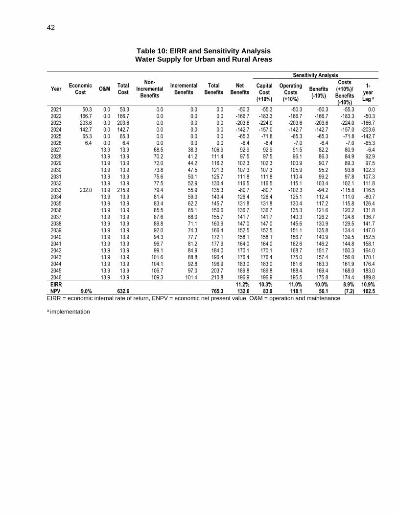
42

Table 10: EIRR and Sensitivity Analysis Water Supply for Urban and Rural Areas

Year Economic

Cost O&M

Total Cost

Non-Incremental

Benefits

Incremental Benefits

Total Benefits

Net Benefits


Capital Cost

(+10%)


Benefits (-10%)


1-year Lag a

2021 50.3 0.0 50.3 0.0 0.0 0.0 -50.3 -55.3 -50.3 -50.3 -55.3 0.0

2022 166.7 0.0 166.7 0.0 0.0 0.0 -166.7 -183.3 -166.7 -166.7 -183.3 -50.3

2023 203.6 0.0 203.6 0.0 0.0 0.0 -203.6 -224.0 -203.6 -203.6 -224.0 -166.7

2024 142.7 0.0 142.7 0.0 0.0 0.0 -142.7 -157.0 -142.7 -142.7 -157.0 -203.6

2025 65.3 0.0 65.3 0.0 0.0 0.0 -65.3 -71.8 -65.3 -65.3 -71.8 -142.7

2026 6.4 0.0 6.4 0.0 0.0 0.0 -6.4 -6.4 -7.0 -6.4 -7.0 -65.3

2027 13.9 13.9 68.5 38.3 106.9 92.9 92.9 91.5 82.2 80.9 -6.4

2028 13.9 13.9 70.2 41.2 111.4 97.5 97.5 96.1 86.3 84.9 92.9

2029 13.9 13.9 72.0 44.2 116.2 102.3 102.3 100.9 90.7 89.3 97.5

2030 13.9 13.9 73.8 47.5 121.3 107.3 107.3 105.9 95.2 93.8 102.3

2031 13.9 13.9 75.6 50.1 125.7 111.8 111.8 110.4 99.2 97.8 107.3

2032 13.9 13.9 77.5 52.9 130.4 116.5 116.5 115.1 103.4 102.1 111.8

2033 202.0 13.9 215.9 79.4 55.9 135.3 -80.7 -80.7 -102.3 -94.2 -115.8 116.5

2034 13.9 13.9 81.4 59.0 140.4 126.4 126.4 125.1 112.4 111.0 -80.7

2035 13.9 13.9 83.4 62.2 145.7 131.8 131.8 130.4 117.2 115.8 126.4

2036 13.9 13.9 85.5 65.1 150.6 136.7 136.7 135.3 121.6 120.2 131.8

2037 13.9 13.9 87.6 68.0 155.7 141.7 141.7 140.3 126.2 124.8 136.7

2038 13.9 13.9 89.8 71.1 160.9 147.0 147.0 145.6 130.9 129.5 141.7

2039 13.9 13.9 92.0 74.3 166.4 152.5 152.5 151.1 135.8 134.4 147.0

2040 13.9 13.9 94.3 77.7 172.1 158.1 158.1 156.7 140.9 139.5 152.5

2041 13.9 13.9 96.7 81.2 177.9 164.0 164.0 162.6 146.2 144.8 158.1

2042 13.9 13.9 99.1 84.9 184.0 170.1 170.1 168.7 151.7 150.3 164.0

2043 13.9 13.9 101.6 88.8 190.4 176.4 176.4 175.0 157.4 156.0 170.1

2044 13.9 13.9 104.1 92.8 196.9 183.0 183.0 181.6 163.3 161.9 176.4

2045 13.9 13.9 106.7 97.0 203.7 189.8 189.8 188.4 169.4 168.0 183.0

2046 13.9 13.9 109.3 101.4 210.8 196.9 196.9 195.5 175.8 174.4 189.8

EIRR 11.2% 10.3% 11.0% 10.0% 8.9% 10.9%

NPV 9.0% 632.6 765.3 132.6 83.9 118.1 56.1 (7.2) 102.5


a implementation

mailto:ENPV@

43

Table 11: EIRR and Sensitivity Analysis Rural Wastewater

Year Economic

Cost O&M

Total Cost

Improved Rural

Wastewater Management

Total Benefits

Net Benefits


Capital Cost

(+10%)


Benefits (-10%)


1-year Lag a

2021 15.9 0.0 15.9 0.0 0.0 -15.9 -17.5 -15.9 -15.9 -17.5 0.0

2022 52.7 0.0 52.7 0.0 0.0 -52.7 -57.9 -52.7 -52.7 -57.9 -15.9

2023 64.4 0.0 64.4 0.0 0.0 -64.4 -70.8 -64.4 -64.4 -70.8 -52.7

2024 45.1 0.0 45.1 0.0 0.0 -45.1 -49.6 -45.1 -45.1 -49.6 -64.4

2025 20.6 0.0 20.6 0.0 0.0 -20.6 -22.7 -20.6 -20.6 -22.7 -45.1

2026 2.0 0.0 2.0 0.0 0.0 -2.0 -2.0 -2.2 -2.0 -2.2 -20.6

2027 20.1 20.1 36.4 36.4 16.3 16.3 14.3 12.7 10.7 -2.0

2028 20.1 20.1 39.9 39.9 19.8 19.8 17.8 15.8 13.8 16.3

2029 20.1 20.1 43.7 43.7 23.6 23.6 21.6 19.2 17.2 19.8

2030 20.1 20.1 47.8 47.8 27.8 27.8 25.7 23.0 21.0 23.6

2031 20.1 20.1 52.4 52.4 32.3 32.3 30.3 27.1 25.1 27.8

2032 20.1 20.1 56.3 56.3 36.2 36.2 34.2 30.6 28.6 32.3

2033 20.1 20.1 60.5 60.5 40.4 40.4 38.4 34.4 32.4 36.2

2034 20.1 20.1 65.0 65.0 45.0 45.0 43.0 38.5 36.5 40.4

2035 20.1 20.1 69.9 69.9 49.8 49.8 47.8 42.8 40.8 45.0

2036 20.1 20.1 75.2 75.2 55.1 55.1 53.1 47.6 45.6 49.8

2037 20.1 20.1 80.0 80.0 59.9 59.9 57.9 51.9 49.9 55.1

2038 20.1 20.1 85.2 85.2 65.1 65.1 63.1 56.6 54.6 59.9

2039 20.1 20.1 90.7 90.7 70.7 70.7 68.7 61.6 59.6 65.1

2040 20.1 20.1 96.6 96.6 76.6 76.6 74.5 66.9 64.9 70.7

2041 20.1 20.1 102.9 102.9 82.8 82.8 80.8 72.6 70.5 76.6

2042 20.1 20.1 109.6 109.6 89.5 89.5 87.5 78.6 76.6 82.8

2043 20.1 20.1 116.8 116.8 96.7 96.7 94.7 85.0 83.0 89.5

2044 20.1 20.1 124.4 124.4 104.3 104.3 102.3 91.9 89.9 96.7

2045 20.1 20.1 132.5 132.5 112.4 112.4 110.4 99.2 97.2 104.3

2046 20.1 20.1 141.2 141.2 121.1 121.1 119.1 107.0 105.0 112.4

EIRR 13.1% 12.3% 12.7% 11.8% 10.5% 12.8%

NPV 9.0% 100.4 85.0 89.3 63.9 37.5 80.3


a implementation

mailto:ENPV@

44

Table 12: EIRR and Sensitivity Analysis

Food Waste and Municipal Sludge Treatment

Year Economic

Cost O&M

Total Cost

Improved Food

Waste and Sludge

Treatment

Total Benefits

Net Benefits


Capital Cost

(+10%)


Benefits (-10%)


1-year Lag a

2021 6.0 0.0 6.0 0.0 0.0 -6.0 -6.6 -6.0 -6.0 -6.6 0.0

2022 20.0 0.0 20.0 0.0 0.0 -20.0 -22.0 -20.0 -20.0 -22.0 -6.0

2023 24.4 0.0 24.4 0.0 0.0 -24.4 -26.8 -24.4 -24.4 -26.8 -20.0

2024 17.1 0.0 17.1 0.0 0.0 -17.1 -18.8 -17.1 -17.1 -18.8 -24.4

2025 7.8 0.0 7.8 0.0 0.0 -7.8 -8.6 -7.8 -7.8 -8.6 -17.1

2026 0.8 0.0 0.8 0.0 0.0 -0.8 -0.8 -0.8 -0.8 -0.8 -7.8

2027 7.6 7.6 24.7 24.7 17.1 17.1 16.4 14.7 13.9 -0.8

2028 7.6 7.6 24.7 24.7 17.1 17.1 16.4 14.7 13.9 17.1

2029 7.6 7.6 24.7 24.7 17.1 17.1 16.4 14.7 13.9 17.1

2030 7.6 7.6 24.7 24.7 17.1 17.1 16.4 14.7 13.9 17.1

2031 7.6 7.6 24.7 24.7 17.1 17.1 16.4 14.7 13.9 17.1

2032 7.6 7.6 24.7 24.7 17.1 17.1 16.4 14.7 13.9 17.1

2033 7.6 7.6 24.7 24.7 17.1 17.1 16.4 14.7 13.9 17.1

2034 7.6 7.6 24.7 24.7 17.1 17.1 16.4 14.7 13.9 17.1

2035 7.6 7.6 24.7 24.7 17.1 17.1 16.4 14.7 13.9 17.1

2036 7.6 7.6 24.7 24.7 17.1 17.1 16.4 14.7 13.9 17.1

2037 7.6 7.6 24.7 24.7 17.1 17.1 16.4 14.7 13.9 17.1

2038 7.6 7.6 24.7 24.7 17.1 17.1 16.4 14.7 13.9 17.1

2039 7.6 7.6 24.7 24.7 17.1 17.1 16.4 14.7 13.9 17.1

2040 7.6 7.6 24.7 24.7 17.1 17.1 16.4 14.7 13.9 17.1

2041 7.6 7.6 24.7 24.7 17.1 17.1 16.4 14.7 13.9 17.1

2042 7.6 7.6 24.7 24.7 17.1 17.1 16.4 14.7 13.9 17.1

2043 7.6 7.6 24.7 24.7 17.1 17.1 16.4 14.7 13.9 17.1

2044 7.6 7.6 24.7 24.7 17.1 17.1 16.4 14.7 13.9 17.1

2045 7.6 7.6 24.7 24.7 17.1 17.1 16.4 14.7 13.9 17.1

2046 7.6 7.6 24.7 24.7 17.1 17.1 16.4 14.7 13.9 17.1

EIRR 14.0% 12.9% 13.5% 12.2% 10.6% 13.9%

NPV 9.0% 34.4 28.5 30.2 20.9 10.9 29.9


a implementation

mailto:ENPV@

45

ANNEX C: RESULTS OF THE CONTINGENT VALUATION STUDY I. Introduction 1. The purpose of this section is to outline the approach and requirements for the conduct of contingent valuation (CV) surveys. The CV method involves directly asking consumers their willingness to pay (WTP) for a service (or a good, usually one that is not marketed) under a given condition. To be able to elicit appropriate responses from consumers on their WTP (values or prices), the given condition is described to the respondents. Thus, consumer responses on WTP values are “contingent or conditioned upon” the delivery of the given service that is described to them, usually an improvement of the existing situation, e.g., intermittent water supply to households to 24 hours a day availability. The WTP values obtained from this survey will be used to estimate the economic benefits of water supply, wastewater and solid waste subprojects. II. Survey Methodology 2. The CV surveys was carried out together with the household social survey. The sampling framework to cover a representative sample of households that will be directly benefiting from the proposed subprojects. A CV survey was conducted for water supply, wastewater and solid waste management subprojects in the county of Xichuan. The subprojects include the water supply for urban and rural areas, wastewater treatment plant in 5 towns (Shangji, Jinhe, Xianghua, Jiuzhong and Houpo) and kitchen waste and municipal sludge co-processing treatment plant. The sampling size is 250 households each for water supply, wastewater and solid waste. The bids were randomly distributed to the respondents. For instance, with 250 respondents and five bids, 50 of the respondents will be asked one bid and another 50 respondents will be asked another bid and so on. The survey includes household characteristics (income, employment, and others), availability and use of public services (water supply, sanitation, solid waste management). 3. The survey instrument was developed based on similar instrument applied in China. About 50 households were interviewed in pretests. Based on the results of pretests, some questions were rephrased and the initial bid distribution was refined. The enumerators were trained on the CV survey. The enumerators were deployed after training and were supervised by the TrTA Social Specialist. The enumerators were trained particularly to ask contingency valuation question in a proper manner, to include a system for ‘callbacks’ (returning to the household for the interview at an appropriate time), to ensure the completeness and quality of results, and review survey implementation, the enumerator must ensure the completeness and quality of results, and should be able review survey implementation according to actual conditions in the field, the survey team should input data and discussion records into laptop computers on a daily basis during the course of the survey. If during the execution of the survey, the selected sample household declined to be interviewed, the survey team shall replace the pre-selected household with one of the five neighbors using counterclockwise rule.

4. A close-ended CV question was used in the survey24. The respondent was asked whether he or she was willing to pay a specified amount that represents the value of the improved services. The CV question was answerable with a “yes” or “no”. The bids were estimated based on the prevailing tariff in the service area. These bids were randomly assigned to respondents of the survey. For the

24 Following guidelines in Gunatilake, et al. ERD Technical Note 19 and 23. ADB. 2007

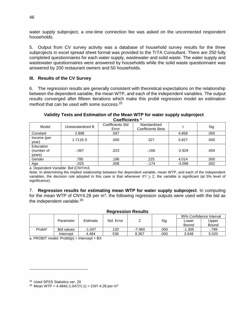
46

water supply subproject, a one-time connection fee was asked on the unconnected respondent households. 5. Output from CV survey activity was a database of household survey results for the three subprojects in excel spread sheet format was provided to the TrTA Consultant. There are 250 fully completed questionnaires for each water supply, wastewater and solid waste. The water supply and wastewater questionnaires were answered by households while the solid waste questionnaire was answered by 200 restaurant owners and 50 households. III. Results of the CV Survey 6. The regression results are generally consistent with theoretical expectations on the relationship between the dependent variable, the mean WTP, and each of the independent variables. The output results converged after fifteen iterations which make this probit regression model an estimation

method that can be used with some success.25 Validity Tests and Estimation of the Mean WTP for water supply subproject

Coefficients a


Error Standardized


Constant 2.898 .597 4.858 .000

Income (per year)

1.711E-5 .000 .327 5.827 .000


-.067 .023 -.166 -2.929 .004

Gender .785 .196 .225 4.014 .000

Age -.025 .008 -.174 -3.098 .002

a. Dependent Variable: Bid (CNY/m3. Note: In determining the implied relationship between the dependent variable, mean WTP, and each of the independent variables, the decision rule adopted in this case is that whenever /t*/ > 2, the variable is significant (at 5% level of significance). 7. Regression results for estimating mean WTP for water supply subproject. In computing for the mean WTP of CNY4.28 per m3, the following regression outputs were used with the bid as

the independent variable.26

Regression Results



Lower Bound

Upper Bound

Probita Bid values -1.047 .132 -7.960 .000 -1.305 -.789

Intercept 4.484 .536 8.367 .000 3.948 5.020


25 Used SPSS Statistics ver. 20 26 Mean WTP = 4.484/(-1.047)*(-1) = CNY 4.28 per m3

47

Validity Tests and Estimation of the Mean WTP for wastewater subproject Coefficients a


Error Standardized


Constant .850 .484 1.757 .080

Income (per year)

-1.777E-6 .000 -.097 -1.522 .129


.009 .009 .064 1.005 .316

Gender -.028 .077 -.023 -.359 .720

Age .006 .003 .111 1.754 0.81

Ethnicity -.793 .417 -.120 -1.902 .058

a. Dependent Variable: Bid (CNY/m3. Note: In determining the implied relationship between the dependent variable, mean WTP, and each of the independent variables, the decision rule adopted in this case is that whenever /t*/ > 2, the variable is significant (at 5% level of significance). 8. Regression results for estimating mean WTP for wastewater subproject. In computing for the mean WTP of CNY1.72 per m3, the following regression outputs were used with the bid as the

independent variable.27

Regression Results



Lower Bound

Upper Bound

Probita Bid values -.646 .101 -6.393 .000 -.845 -.448

Intercept 1.113 .286 3.889 .000 .827 1.399


Validity Tests and Estimation of the Mean WTP for solid waste subproject Coefficientsa


Error Standardized


Constant .432 .282 1.535 .126

Income (per year)

-4.865E-6 .000 -.424 -7.296 .000


.002 .005 .028 .473 .637

Gender .035 .044 .046 .788 .432

Age .000 .002 .010 .167 .868

Ethnicity .028 .243 .007 .115 .908

a. Dependent Variable: Bid (CNY/m/3. Note: In determining the implied relationship between the dependent variable, mean WTP, and each of the independent variables, the decision rule adopted in this case is that whenever /t*/ > 2, the variable is significant (at 5% level of significance).

27 Mean WTP = 1.113/(-.646)*(-1) = 1.72/m3

48

9. Regression results for estimating mean WTP for solid waste management subproject. Mean WTP cannot be computed, lowest bid CNY20 per month got 19 Yes response while No responses for all the other remaining.

APPENDIX 1

WTP QUESTIONNAIRE Assessment of existing wastewater management services (integrated in the household survey questionnaire) 1. Are you connected to the sewerage network? ___1) Yes __ 2) No 2. Do you have a septic tank? ___ 1) Yes ___ 2) No If yes, is it _____1) individual ______2) communal 2.1 How often do you empty your septic tank? __ 1) per month ___ 2) per year 2.2 How much do you spend in a year to maintain your septic tank? ___ RMB 3. If you do not have a septic tank, how do you dispose of your wastewater? 1 Flows to the backyard ____ 2 Drains directly to the rivers and waterways ___ 3 Drains to the sewerage pipelines ___ 4 Others, please indicate ___ 4. What is your source of water supply? __ 1) Municipal system ___ 2) Deep well (500 meters and above) ___ 3) Shallow well (120 to 200 meters) ____ 4) Both municipal system and well 5. Are you satisfied with the existing sewage disposal system? ___ 1) Yes ___ 2) No 6. If not, how have you been affected by the poor disposal system? Please check all that are applicable.

Please check

1) Toxic smell coming from wastewater pool in your backyard or polluted river

How many meters away is your house from the polluted water? ___

2) Polluted water supply How much did you spend for constructing a deep well? ___ CNY How much do you spend in a year to maintain the deep well? ___ CNY a year

3) Presence of flies and mosquitoes in your surroundings

How much has your livelihood been affected because of unsanitary environment (e.g., for restaurants)? __ CNY a year

4) Poor quality of agricultural produce How much is your loss in income in a year due to polluted water used for irrigation? ___ CNY a year

5) Increase in illnesses and diseases How many times in a year have you or your family fall sick because of the polluted surroundings? __ How much have you spent in a year for medical expenses due to these illnesses? ___ CNY a year

Assessment of existing solid waste management services (integrated in the household survey questionnaire) Distance to the proposed waste processing site ---- meters

49

How do you dispose your daily domestic garbage? 1. Collected from my house ____ 2. Dump out of the house ______ 3. Dump into public garbage tank ____ 4. Dump into river ____ 5. Use to feed poultry and livestock (chicken, pig, etc.) ____ 6. Burning waste ____ 7. Composting in a traditional pit ___ 8. Other (please specify) ____ How frequent is the collection of garbage? 1. Daily ____ 2. Every other day______ 3. Once a week ___ 4. Twice a week ___ 5. Others (please specify) ___ How far do you to walk to dispose of your garbage? 1. Within the yard___ 2. Outside the yard, nearby ___ 3. Far away ___ Are you satisfied with the current solid waste management system? 1. Fully Satisfied ___ 2. Satisfied ____ 3 Neutral ___ 3. Unsatisfied___ 4. Extremely unsatisfied ___ In your view how have you been affected by the poor solid waste management system? Please check all that are applicable.

Please check

1. Toxic smell coming from your backyard or polluted river

How many meters away is your house from the polluted water? ___

2. Presence of flies and mosquitoes in your surroundings

How much has your livelihood been affected because of unsanitary environment (e.g., for restaurants)? __ CNY a year

3. Poor quality of agricultural produce

How much is your loss in income in a year due to polluted water used for irrigation? ___ CNY in a year

4. Increase in illnesses and diseases

How many times in a year have you or your family fall sick because of the polluted surroundings? __ How much have you spent in a year for medical expenses due to these illnesses? ___ CNY a year

Assessment of existing water supply service (integrated in the household survey questionnaire) 1. Are you connected to the municipal water supply system? ___ 1) Yes ___ 2) No (If no, go to question numbers 18 – 21.) 2. If yes, do you receive continuous water supply during the day? ___ 1) Yes ___ 2) No 3. If no, how many hours in a day do you receive water ___ (hours) and what times of the day do you receive water? ____

50

4. Can you drink your tap water without boiling and filtering? __ 1) Yes ___ 2) No 5. How do you rate the quality of water from the tap?

Extremely unsatisfied (1)

Moderately unsatisfied (2)

Neutral (3)

Moderately satisfied (4)

Extremely satisfied (5)

Appearance (e.g. turbid, brown color)

Smell

Taste

Overall satisfaction

6. How much do you spend, if any, on the following items in a month?

Item Amount (CNY)

Boiling (number of pots per day)

Source of energy:

1. Coal

2. Firewood

3. Liquid Gas

4. Electricity

Cost (water boiling) per month

Filters (initial cost)

Treatment per month

Others

Total

7. Do you have a water storage tank 1) Yes ____ 2) No _______ If yes what was the cost CNY ________ Age of the tank ________ 8. What is your family’s monthly water bill? CNY___ 8.1 How much is your family’s average monthly water consumption from the municipal water supply system? ___ m3 9. Is the water that you receive from the municipal water supply system sufficient for your basic living needs? ___ 1) Yes ___ 2) No 10. Is there enough water to be used for gardening and other purposes? 1) Yes __ 2) No __ 11. If no, please indicate below how you supply for your additional water needs. Please check all that are applicable.

Please check

1) I have a private well. Please indicate the depth of the well _______

What is the cost of construction? CNY___ Year of construction __________

2) I buy bottled water How much do you spend in a month? CNY___

3) I buy water from others’ wells.

How far is the place from your house? ___ nearest (meters) ____ farthest (meters) _______ How many times per week do you fetch water in dry season? ____ wet season? _______

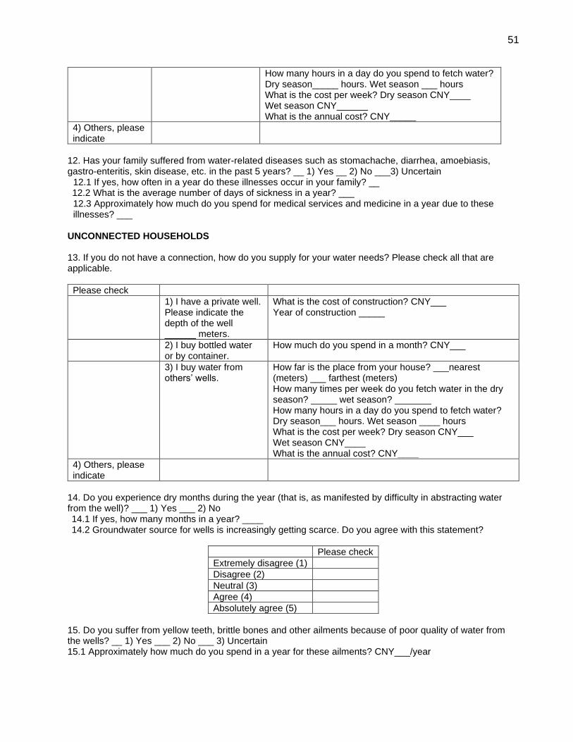
51

How many hours in a day do you spend to fetch water? Dry season_____ hours. Wet season ___ hours What is the cost per week? Dry season CNY____ Wet season CNY______ What is the annual cost? CNY_____

4) Others, please indicate

12. Has your family suffered from water-related diseases such as stomachache, diarrhea, amoebiasis, gastro-enteritis, skin disease, etc. in the past 5 years? __ 1) Yes __ 2) No ___3) Uncertain

12.1 If yes, how often in a year do these illnesses occur in your family? __ 12.2 What is the average number of days of sickness in a year? ___ 12.3 Approximately how much do you spend for medical services and medicine in a year due to these illnesses? ___

UNCONNECTED HOUSEHOLDS 13. If you do not have a connection, how do you supply for your water needs? Please check all that are applicable.

Please check

1) I have a private well. Please indicate the depth of the well ______ meters.

What is the cost of construction? CNY___ Year of construction _____

2) I buy bottled water or by container.

How much do you spend in a month? CNY___

3) I buy water from others’ wells.

How far is the place from your house? ___nearest (meters) ___ farthest (meters) How many times per week do you fetch water in the dry season? _____ wet season? _______ How many hours in a day do you spend to fetch water? Dry season___ hours. Wet season ____ hours What is the cost per week? Dry season CNY___ Wet season CNY____ What is the annual cost? CNY____

4) Others, please indicate

14. Do you experience dry months during the year (that is, as manifested by difficulty in abstracting water from the well)? ___ 1) Yes ___ 2) No 14.1 If yes, how many months in a year? ____ 14.2 Groundwater source for wells is increasingly getting scarce. Do you agree with this statement?

Please check

Extremely disagree (1)

Disagree (2)

Neutral (3)

Agree (4)

Absolutely agree (5)

15. Do you suffer from yellow teeth, brittle bones and other ailments because of poor quality of water from the wells? __ 1) Yes ___ 2) No ___ 3) Uncertain 15.1 Approximately how much do you spend in a year for these ailments? CNY___/year

52

D.1

Contingent Valuation Scenario - Rural Wastewater Treatment Plant The proposed project will help to improve the water resources situation, the living conditions of residents and the physical environment of Xichuan. The proposed project involves the construction of individual sewage treatment facility and sewage pipelines. This way sewage would be treated before discharging to the rivers. The water resources situation in your area is expected to improve which means safe, less polluted ground and surface waters, cleaner surroundings with less breeding grounds for flies and mosquitoes, cleaner water available for agricultural irrigation purpose and less stress on water resources. However, to be able to realize these improvements, it entails costs. The costs would have to be shared between the government and the beneficiaries.

D.1.1

Given these proposed improvements in the service, would you like to pay (CNY1.5 | CNY2.5 | CNY3.0 | CNY4.0| CNY5.0) per cubic meter for the wastewater services to be provided under the Project.

1. Yes 2. No

囗

囗

D.1.2

If answer is Yes, could you please explain your reasons.

1. I really want/need the service because it benefits my household.

2. The tariff is not too high. 3. As a responsible citizen, I should

contribute to a cleaner environment. 4. Others, please specify

__________________ 5. Don’t know/not sure

D.1.3 If answer is No, could you please explain your reasons for not agreeing to pay the tariff.

1. I do not really want/need the improved service, because the Project does not benefit my household.

2. I don’t believe wastewater is a serious problem in town.

3. There are other priorities for my household.

4. The tariff is too high. I cannot afford it. 5. Others, please specify ____ 6. Don’t know/not sure

D.2

Contingent Valuation Scenario - Rural Solid Waste Management With the population growing, the government foresees that the solid waste services situation will worsen in the next years if no intervention will be made soon to address the situation. The intention was to address environmental pollution caused by garbage of households flowing into the waterways. The rivers have become silted over time which has affected the normal drainage for rainwater and has caused water in these waterways to remain stagnant. At the household level, there is the risk of disease from unsanitary environment. Poor garbage disposal system has also polluted groundwater which is a source of water supply and surface water which is used for irrigating farmlands. However, to be able to realize these improvements, it entails costs. The costs would have to be shared between the government and the beneficiaries.

D.2.1

Given these proposed improvements in the service, would you like to pay (CNY20 | CNY40 | CNY60 | CNY80 | CNY100) per month for the solid waste management services to be provided under the Project.

1. Yes 2. No

囗

囗

53

D.2.2


1. I really want/need the improved service because it benefits my household.

2. The tariff is not too high. 3. As a responsible citizen, I should

contribute to a cleaner environment. 4. Others, please specify


D.2.3 If answer is No, could you please explain your reasons for not agreeing to pay the tariff.


2. I don’t believe solid waste is a serious problem in town.


4. The tariff is too high. I cannot afford it. 5. Others, please specify ____

Don’t know/not sure

D.3

Contingent Valuation Scenario – Rural Water Supply With the population growing, the government foresees that the water supply situation in the town will worsen in the next years if no intervention is made soon to address the situation. Thus, the government will improve the water supply service in the town including extending the service to other areas. Water will also be treated to make it safe for human consumption, tap water will be according to national drinking water standards and therefore will not need boiling, filtering or treating, water will be available 24 hours a day and so there will be no need to stay up late at night and to store water. More households will be connected so there will be no need to invest on shallow wells or maintain existing wells. This will prevent further pollution of groundwater sources. It is expected that there will be fewer incidences of water related diseases due to poor water quality and hygiene. However, to be able to realize these improvements, it entails costs. The costs would have to be shared between the government and the beneficiaries.

(The Enumerator proceeds to ask the following questions, if the household is currently connected)

D.3.1

Given these proposed improvements in service, if water is available for 24 hours, would you increase water consumption?

1. Yes 2. No If so by how much _________%

囗

囗

D.3.2

To provide the improved water services, it will cost more to Water Supply Company, are you willing to pay an additional amount of (CNY1.5 | CNY2.5 | CNY3.5 | CNY4.0 | CNY5.0) per cubic meter to have the improved water service to be provided by the Project?

1. Yes 2. No

囗

囗

54

D.3.3



2. The increase in tariff is not too high. 3. I am worried about the health risks of

my existing water source. 4. Others, please specify


D.3.4 If no, would you disconnect from the water supply system?

1. Yes 2. No

囗

囗

D.3.5 Please explain your reasons for not agreeing to pay the additional tariff.


2. I don’t believe water supply is a serious problem in town.


4. The increase in tariff is too high. I cannot afford it.

5. Others, please specify ____ 6. Don’t know/not sure

D.3.6

If you would disconnect to the water network, where do you think your household would obtain your water supplies?

1. Private well 2. Neighbors 3. Vendors and Tankers 4. Others, please specify ____ 5. Don’t know/not sure

(The Enumerator proceeds to ask the following questions, if the household is currently not connected)

D.3.7

In order to access the improved service, it would cost your household CNY 700.00 one-time connection charge for water meter and pipelines. In addition, you will have to pay (CNY1.5 | CNY2.5 | CNY3.5 | CNY4.0 | CNY5.0) per cubic meter on monthly basis. Would you be willing to connect to the improved water supply system?

1. Yes 2. No

囗

囗

D.3.8 If answer is Yes, could you please explain your reasons.


2. The tariff is not too high. 3. I am worried about the health risks of

my existing water source. 4. Others, please specify


55

D.3.9 If answer is No, could you please explain to me your main reasons for not connecting to the network.

1. I do not really want/need the improved service.

2. The monthly water bill is affordable but connection charge is too high.

3. The water tariff is too high. I cannot afford it.

4. I am not worried about the health risks of my existing water source.

5. I am happy with my water source 6. Others, please specify ____ Don’t know/not sure

D.3.10

If no to question D.3.7 will you accept the service if there is an easy instalment payment system to pay the connection charge?

1. Yes 2. No

囗

囗