design, simulation and analysis of an air-conditioning

Proceedings of 8th IOE Graduate ConferencePeer Reviewed

ISSN: 2350-8914 (Online), 2350-8906 (Print)Year: 2020 Month: June Volume: 8

Design, Simulation and Analysis of an Air-Conditioning System:A Case Study of the Proposed Aerospace Building of PulchwokEngineering Campus in the Context of Nepal

Sudin Bhuju Shrestha a, Hari Bahadur Dura b, Nawraj Bhattarai c

a, b, cDepartment of Mechanical and Aerospace Engineering, Pulchowk Campus, IOE, TU, NepalCorresponding Email:[email protected], [email protected], [email protected]

AbstractOptimization of energy consumption has been on the lime light from the beginning of this 21st century, withmore than half of the energy being spent on controlling indoor atmospheric condition. Taking into accountthat the field of Heating, Ventilation and Air-conditioning (HVAC) is in its preliminary developing stage inNepal, researches associated to HVAC system optimization is only starting to germinate with detailed HVACoptimization studies being implied only in major HVAC projects. Commercially available software are availablefor that however, they only do so much in predicting the load not so much on how that load will affect thetemperature distribution with respect to time and space. At such Computational fluid dynamics (CFD) canbe a very effective tool in simulating the steady and unsteady temperature distributions. The present workfocuses on design, simulation and analysis of an air conditioning system best suited for the auditorium hall ofthe proposed Aerospace building of the Pulchwok Engineering Campus. Considering the fact, that the climateof Kathmandu is of subtropical type, the cooling loads were calculated for summer months from March toOctober via various methods implying Cooling Load Temperature Differences(CLTD), Hourly Analysis Program(HAP) and Autodesk RevitMEP. Consequently the loads were estimated to be 9.87 Tons, 8.52 Tons and 9.487Tons respectively. Simulations were then performed in Fluent ANSYS for boundary conditions meeting therequirements of the weather data for 8, 9, 10 and 11 Tons of air-conditioning system setups which led tothe conclusion that for desired design temperature of 21.5ºC, 10 Tons had the best performance in terms ofaverage of kWh used per hour for comfortable condition as well as the total energy consumed.

KeywordsCFD, Fluent, RevitMEP, Radiant Time Series, Houly Analysis Program, Conduction Transfer Function, CoolingLoad Temperature Difference, Air Conditioning

1. Introduction

With the exponential growth of the world’s economy,the problem of insufficient power supply has takenplace in many countries in recent years, especiallyduring the peak period where building energyconsumption accounted for 40% of the total energyconsumption in the world while the air-conditioningsystems in buildings consume about 60% to 70% oftotal electricity consumption in some countries andcontribute over 30% of the CO2 emissions [1, 2]. Thisincreasing demand for heating, cooling and electricitysupplies in buildings stimulates the search forhigher-more efficient and low-emission energyproduction, conservation and usage methods [3].

Located at 27°4′N 85°21′E and an elevation of1338m, Kathmandu valley is located in the warmtemperate zone (1,200m-2,300m). The averagesummer temperature varies from 28°C to 30°C (82°Fto 86°F) while the average winter temperature is10.1°C (50.2°F) in the valley [4, 5]. Similarly, whilethe highest temperature in summer reaches to about32.5°C, lowest temperature reaches to about -2°C [6].Because of this type of climatic conditionsKathmandu valley in general faces about 8 months ofsummer (March to October) and 4 months of winter(November to February). Moreover, in this type ofclimatic conditions the cooling load during thesummer days are much higher than the heating loadduring the winter. As a result, the HVAC systems

Pages: 923 – 931

Design, Simulation and Analysis of an Air-Conditioning System: A Case Study of the ProposedAerospace Building of Pulchwok Engineering Campus in the Context of Nepal

installed in the valley are designed prioritizing thesummer cooling load conditions. In Kathmandu valleyalone, energy demand of residential sector was foundto be about 7,500 TJ in 2013 with increase at the rateof 4% per annum. About 4% of total energyconsumed in an urban house in the country is forpurpose of space heating and cooling [7]. One of thedifficult aspects of estimating the maximum coolingload for a space is determining the time at which thismaximum load will occur. The walls and roof thatmake up a building’s envelope have the capacity tostore heat energy which causes the time lag for theheat transfer from outdoors to the space. As a resultindividual components that make up the space coolingload often peak at different times of the day, or evendifferent months of the year. [8]. HVAC is the totalstudy of the systems which regulates, controls andmaintain the required atmospheric condition of anindoor or vehicular environment irrespective ofexternal conditions [9]. Application of CFD in thestudy area of HVAC is not new. Simulations byEXACT3 CFD code were carried out to analyze theperformance of split-type air conditioners with respectto the temperature rise of condensing units installed atbuilding re-entrant and it was reported that CFDtechnique is capable of providing accurate resultsassociated to the stack effect on the performance ofthe AC units serving at different floors of thebuilding [10]. Analysis of the feasibility and energysaving property of clean air conditioning technologyin clean operating rooms in a hospital where air flowdistribution was simulated using the CFD softwareAirpak 3.0 and Fluent and it was found that anincrease of the air supply area and return air inlets canincrease the area of unidirectional flow regions of themain flow regions and avoid indoor vortexes andturbulivity in the operating area as well as theapplication of a secondary air return system insummers can reduce energy consumption [11].

Despite the effectiveness of CFD in the field ofHVAC, CFD is still very new to the Nepalese sciencesociety. It all boils down to the fact that the immenseamount of computational resources required for CFDcalculations which are not readily accessible to allhere. Consequently, the application of CFD in HVACis only limitedly applied on large commercial HVACproject in which access to computational resources arepossible.

1.1 Governing equations

The governing equations for three-dimensional, steady,turbulent and incompressible flow with heat transferare given by the known continuity equation, the energyequation, N–S equation (momentum equation).Continuity equation:-

∂ p∂ t

+∇ · (ρu) = 0 (1.1)

Momentum equation (N-S equation):-

∂u∂ t

+u.∇u =V ∇2u− 1

ρ∇p+ρg (1.2)

Energy equation:-

∂

∂ t

(ρ

(e+

V 2

2

)+∇ ·

(ρ

(e+

V 2

2

)·V)

+∇ · (p∨)− viscous force +∇ · (q) = 0 (1.3)

where,

u,v, w =Velocity of fluid in X, Y and Z directions

ρ , µ , ∇, p =Density, Viscosity, Divergence and Pressure

1.2 Heat gain and cooling load calculationmethods

1.2.1 Cooling Load Temperature Difference(CLTD)

The CLTD method accounts for the thermal response(lag) in the heat transfer through the wall or roof, aswell as the response (lag) due to the radiation of partof the energy from the interior surface of the wall tothe object within the space which varies with heatgain with time, the massiveness of the structure, andthe geographical location [12]. The total classificationof 41 walls and 42 roofs in CTF method wassimplified and a practical usable version of the CLTDtables was described(10 roofs and 16 walls) in GRP158 [13] which is based on work done by [14]. TheCLTD values corresponded to the heat gain caused byoutdoor air temperature and solar radiation under a setof standard conditions, which included a latitude of40°N, date of July 21, maximum outdoor temperatureof 95°F, daily temperature range of 21°F, and aninside design temperature of 78°F and to calculate forother locations latitude and month correction factorwere provided to use. Later on however separatetables for latitude 24°N, 36°N and 48°N were devisedavoiding the need for latitude and month correctionfactor. The equations involved in calculation of loadusing CLTD are as follows.a) External walls and roofs:-

qθ1 =UA(CLT D)corr θ (1.4)

924

Proceedings of 8th IOE Graduate Conference

(CLT D)corr θ = [(CLT D∗K)

+(78− t i)+(tom−85)]∗ f (1.5)

tom = to−DR2

(1.6)

b) Internal partition walls and floor:-

qθ2 =UA(to− tr) (1.7)

c) Solar gain through glass:-

qθ2 = A(SC)(SCL)θ

(1.8)

d) Conductive heat gain through glass:-

qθ3 =UA(to− tr) (1.9)

e) People:-

qθs4= N(sensibleheatgain)(CLF) (1.10)

qθL4= N( Latent heat gain) (1.11)

qθ4 = qθs4 + qθ14 (1.12)

f) Lights:-

qθ5 = N(BF)(W )(CLF) (1.13)

g) Equipments:-

qθ6 = N(UF)(W )(CLF) (1.14)

h) Ventilation and infiltration air load estimation:-

qθs7= m(cp)(to− tr) (1.15)

qθ17 = m(hg)(W 1−W 2) (1.16)

qθ7 = qθs7 + qθ17 (1.17)

V = Aleak

√as (to− tr)+awv2 (1.18)

where,

A = Area, ft2 or m2

CLTDcort θ = Corrected CLTD which gives the temperature differenceequating to the cooling load at temp θ ,0 F or 0C

CLTD = Tabular CLTD, oF or oC

ti and tom = Actual inside and mean outside design dry bulbtemperature, oF or oC

DR = Daily range, oF or oC

K = Colour adjustment factor, 1 if dark coloured or light in anindustrial area,0.83 if permanently medium coloured (rural area), 0.65if permanently light-coloured (rural area) (ASHRAE, 1980)

U= Overall heat transfer coefficient, Btu/(hrft2oF

)or W/

(m2oC

)to = Temperature in adjacent space or exterior environment, ◦F or ◦C

tc = Inside design temperature (constant) in conditioned space, ◦F or◦C

SC = Shading coefficient (internal shade)

SCLθ = Solar cooling load factor, Btu/(hr-ft2◦F ) or W/(m2◦C

)qθs4 and qθ14 = Sensible and latent heat load from people

CLF = cooling load factor

N = number of respective element

BF = Ballast factor, 1.0 for incandescent bulb and 1.2 for fluorescentlight

W = Watts input from electrical plans or lighting fixture data, Btu/hr

UF = Usage factor

qθs7 and qθ17 = Sensible and latent heat load from infiltration

m = Mass flow rate of ventilation/infiltration air, kg/sec or 1b/hr

Cp = Specific heat of air at constant pressure, J/kg or Btu/lb

hg = latent heat of vaporization, J/kg or Btu/lb

W1−W2 = Difference of specific humidity, g/kg or oz/lb

Aleak = Effective leakage (ELA), cm2 or in2

as = Stack coefficient [15],[(L/s)2/

(cm4 ·K

)]or[(

ft3/min)2/in4 ·o F

)]aW = Wind coefficient [15],[(L/s)2/

(cm4 · (m/s)2

)]or[(

ft3/min)2/in4 · (mph)2

)]v = Wind speed, m/s or mph

1.2.2 Conduction Transfer Function Model

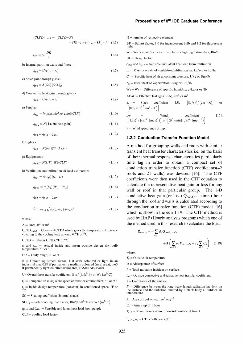
A method for grouping walls and roofs with similartransient heat transfer characteristics i.e. on the basisof their thermal response characteristics particularlytime lag in order to obtain a compact set ofconduction transfer function (CTF) coefficients(42roofs and 21 walls) was devised [16]. The CTFcoefficients were then used in the CTF equation tocalculate the representative heat gain or loss for anywall or roof in that particular group. The 1-Dconductive heat gain (or loss) Qcond,t at time t hourthrough the roof and walls is calculated according tothe conduction transfer function (CTF) model [16]which is show in the eqn 1.19. The CTF method isused by HAP (Hourly analysis program) which one ofthe method used in this research to calculate the load.

Qcond,t =−∑n≥1

dnQcond,t−n∆t

+A

(∑n≥0

bnT os,t−n∆t −T i ∑n≥0

Cn

)(1.19)

where,

To = Outside air temperature

α = Absorptance of surface

It = Total radiation incident on surface

ho = Outside convective and radiative heat transfer coefficient

ε = Emmitance of the surface

F = Difference between the long-wave length radiation incident onthe surface and the radiation emitted by a black body at outdoor airtemperature

A = Area of roof or wall, m2 or f t2

4t = time step of 1 hour

Tos,t = Sol–air temperature of outside surface at time t

bn,cn,dn = CTF coefficients [16]

925


1.2.3 Radiant Time-Series Method

The RTSM method makes simplifications such asthere is no internal or external heat balance rather it isassumed all the surface are effectively at the zone airtemperature and thus facilities the use of singleconvection coefficients, radiation coefficients as wellas fixed surface conductance independent of surfacetemperature, sky temperature etc. [15]. The storageand release of energy by the surfaces areapproximated with predetermined zone responsevalues. The RTSM method if heat load calculation isused by Autodesk RevitMEP software which isanother method used to calculate the heat load in thisresearch. The basic equations involved in the RTSmethods are given below.

q′′convection,ext, j,θ = hc(te− tos, j,θ

)(1.20)

te = to +αGt /ho −

εδR /ho (1.21)

q′′conduction,in, j,θ =23

∑n=0

Y pn(te, j,θ−nδ − trc

)(1.22)

where,

ho = Combined exterior convection and radiation coefficients,Btu/hrft2F or W/m2K

δR = Difference between thermal radiation incident on the surfacefrom the sky and surroundings and the radiation emitted by ablackbody at outdoor air temperature, Btu/hrft2 or W/m2

Ypn = nth response factor, Btu/hrft2F or W/m2K

te, j,θ−nδ = Sol-air temperature, n hours ago, F or C

trc = Presumed constant room air temperature, F or C

2. Methods and Methodology

2.1 Description of the Auditorium Hall

Table 1: Information related to the Auditorium Hall

S.N. Element Value1. Floor area 3585.0ft2

2. Floor size 68.1ft × 49.2ft3. Roof area 3596.4ft2

4. Roof exposure NW5. Roof slope 5 degrees6. Average ceiling height 25.3ft7. Location of Partition SW side8. Location of hall NE side of the building9. Longer Side NE, SW10. Shorter side NW, SE11. Floor location of the hall 2nd floor12. Total number of floors occupied 2nd and 3rd

13. Probable location of window placement NW and NE side.14. Door width 5ft

Table 2: Monthly temperature pattern for KathmanduValley (°F) (ASHRAE, 1993)

Month Max DBT Min DBT Max WBT Min WBTJan 77.2 52.2 70.6 51.7Feb 79.2 54.2 71.6 53.7Mar 82.4 57.4 74.8 56.9Apr 83.6 58.6 75.0 58.1May 86.0 61.0 76.0 60.5Jun 88.0 63.0 78.0 62.5Jul 89.0 64.0 78.0 63.5Aug 89.0 64.0 78.0 63.5Sep 87.0 62.0 77.0 61.5Oct 84.8 59.8 75.8 59.3Nov 80.6 55.6 73.8 55.1Dec 78.2 53.2 71.8 52.7

2.2 Considerations Made

2.2.1 Material Assumptions

Table 3: Load element assumptions

Element R-value (hrft2oF/Btu)Wall 5.621 (Type 12)Roof 14.48 (Type 4)Floor 2.129Door 1.41206Window 1.03891 (SC 0.6 Zone type C)Number of occupancy 100 (Per person 350 Btu/hr)Lighting 0.9 W/ft2

Infiltration 91.9301 CFM (Calculated)Electrical appliance 20% of 16A/220V supply lost as heat

2.2.2 Inlet and Return Vent Parameters

Table 4: Return-vent parameters

S.N. Tons A/C arrangement CFM Return ventsize (in2)1 Ton 2 ton

1. 8 4 2966.4 1053.7483. 9 1 4 3407.8 1209.5775. 10 5 3708 1315.5577. 11 1 5 4308.2 1527.448

Table 5: Inlet-vent parameters

Capacity 1.083 Tons 2.041 TonsArea(mm) 900*100 1000*100CFM 441.4 741.6Velocity (m2/s) 2.314 3.499Temp. of air exiting (oC) 16.83 15.03Watts 1095 2010

The sizing of the return vent in based on (EngineeringToolBox, 2010). While the inlet vent parameters arebased on the split air-conditioner models found in themarket manufactured by LG (VM242H6 andVM122H6).

926


2.2.3 Boundary Conditions

The wall boundary conditions were set up based onthe type of material and the weather conditions.Radiation boundary condition was chosen assumingthat the outer surface of the wall is in equaltemperature as the ambient. For representing the heatgeneration through occupants inside the auditorium,heat generation markers of diameter 30cm wereplaced equidistant to each other (in total of 52markers) and heat flux of 100 occupants are assumedto be produced from them. Velocity inlets were setupfor each vents as mentioned in the table 5. Similarlyfor the return vent (outlet-vent) boundary conditionwas chosen in ANSYS with non-existent backflowpressure and backflow temperature of the ambientspace.

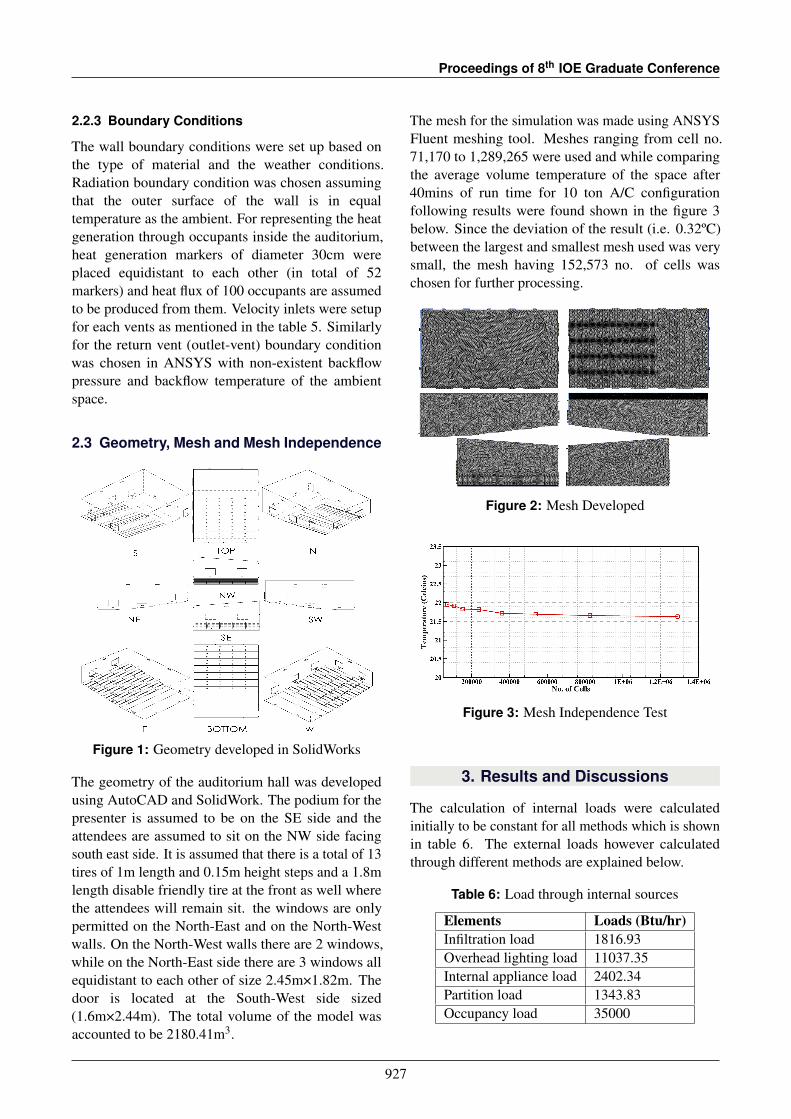
2.3 Geometry, Mesh and Mesh Independence

Figure 1: Geometry developed in SolidWorks

The geometry of the auditorium hall was developedusing AutoCAD and SolidWork. The podium for thepresenter is assumed to be on the SE side and theattendees are assumed to sit on the NW side facingsouth east side. It is assumed that there is a total of 13tires of 1m length and 0.15m height steps and a 1.8mlength disable friendly tire at the front as well wherethe attendees will remain sit. the windows are onlypermitted on the North-East and on the North-Westwalls. On the North-West walls there are 2 windows,while on the North-East side there are 3 windows allequidistant to each other of size 2.45m×1.82m. Thedoor is located at the South-West side sized(1.6m×2.44m). The total volume of the model wasaccounted to be 2180.41m3.

The mesh for the simulation was made using ANSYSFluent meshing tool. Meshes ranging from cell no.71,170 to 1,289,265 were used and while comparingthe average volume temperature of the space after40mins of run time for 10 ton A/C configurationfollowing results were found shown in the figure 3below. Since the deviation of the result (i.e. 0.32ºC)between the largest and smallest mesh used was verysmall, the mesh having 152,573 no. of cells waschosen for further processing.

Figure 2: Mesh Developed

Figure 3: Mesh Independence Test

3. Results and Discussions

The calculation of internal loads were calculatedinitially to be constant for all methods which is shownin table 6. The external loads however calculatedthrough different methods are explained below.

Table 6: Load through internal sources

Elements Loads (Btu/hr)Infiltration load 1816.93Overhead lighting load 11037.35Internal appliance load 2402.34Partition load 1343.83Occupancy load 35000

927


3.1 Cooling Load Temperature Difference

By using the CLTD method the maximum load for theJuly and August month was calcualed to be 9.87 Tonsat 5pm in the evening. The breakdown of individualexternal loads as well as montlhy load calculated areshown below.

Figure 4: Hourly heat transfer for July (CLTD)

Table 7: External load by CLTD

Element Load (Btu/hr)Wall 18938.40Roof 19372.87Floor 15155.00Door 509.89Window 12868.27Partition Load 1343.83

Figure 5: Monthly load pattern (CLTD)

3.2 Hourly Analysis Program

Unlike CLTD which uses only one temperature value,HAP takes into consideration of the hourly varyingtemperature through the day. By doing so themaximum load was calculated to be 8.52 Tons at 5pmin the month of July/August. To make equivalentcomparisons to CLTD, assumptions were made.Assump 1: the peak design temp. is reached at thepeak load time (5pm) and Assump 2: the peak designtemp. occurs throughout the day. The maximum load

calculated by HAP using Assump:1 and Assump:2were 8.7 Tons and 9.1 Tons respectively.

Table 8: External load by HAP(CTF) Btu/hr

Element Hourly temp. Assum.1 Assum.2Wall 17277 17325 20043Roof 13226 13228 14081Window 10294 10691 10910Door 350 399 426Floor 10004 11580 12450Partition 887 1027 1104

Figure 6: Monthly load pattern (HAP)

3.3 RevitMEP

The total load was calculated to be about 9.487 Tonsat 5pm of July respectively. It is to be noted thatRevitMEP is only able calculates the design maximumcooling load and hourly or month wise load generationis not possible.

Table 9: External load by RevitMEP(RTSM)

Elements Loads (Btu/hr)Walls 18109.40Windows 13382.10Door 41.50Roof 16907.31Floor 15155Total 63595.31

3.4 CFD Results

The simulations were performed for various A/C Tonconfigurations for March to October. For assisting thesimulation as well as the analysis, it was assumed thatthe human comfort conditions to begin below 23.5ºCand final desired inner targeted temperature conditionsto be multiple one; being 22.5ºC, 22ºC and 21.5ºC.

Considering the response time, in all cases of desiredinner temperature, it was found that the performance

928


ranged from the highest A/C configuration i.e. 11Tons to cool the quickest while the 8 Tons to be theslowest, which was obvious. The 8 Ton A/Cconfiguration was not able to cool down thetemperature of the space to 21.5ºC. The 8 Ton A/Cconfiguration suffered significant performance loss inthe month of July and August being able to drop thetemperature to human comfort range only after the30-40 minute mark, yet never able to attain the 21.5ºC.However, in other months overall it is able to droptemperature to human comfort range within 15-25minutes.

Figure 7: 8 Ton A/C performance


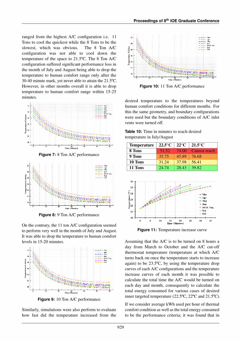
On the contrary, the 11 ton A/C configuration seemedto perform very well in the month of July and August.It was able to drop the temperature to human comfortlevels in 15-20 minutes.


Similarly, simulations were also perform to evaluatehow fast did the temperature increased from the


desired temperature to the temperatures beyondhuman comfort conditions for different months. Forthis the same geometry, and boundary configurationswere used but the boundary conditions of A/C inletvents were turned off.

Table 10: Time in minutes to reach desiredtemperature in July/August

Temperature 22.5°C 22°C 21.5°C8 Tons 51.52 74.00 Cannot reach9 Tons 35.75 45.89 76.6810 Tons 31.24 37.98 56.4111 Tons 24.74 28.43 39.82

Figure 11: Temperature increase curve

Assuming that the A/C is to be turned on 8 hours aday from March to October and the A/C cut-offthermostat temperature (temperature at which A/Cturns back on once the temperature starts to increaseagain) to be 23.5ºC, by using the temperature dropcurves of each A/C configurations and the temperatureincrease curves of each month it was possible tocalculate the total time the A/C would be turned oneach day and month, consequently to calculate thetotal energy consumed for various cases of desiredinner targeted temperature (22.5ºC, 22ºC and 21.5ºC).

If we consider average kWh used per hour of thermalcomfort condition as well as the total energy consumedto be the performance criteria; it was found that in

929


the case of 22.5ºC (desired inside temperature), theperformance was in the order of 8, 10, 11 and 9 Tons.In the case of 22ºC (desired inside temperature), theperformance was in the order of 8, 11, 10 and 9 Tons.While in the case of 21.ºC (desired inside temperature),the performance was in the order of 10, 11, 9 and 8Tons.

Table 11: Total kWh used for cooling

Temperature 22.5°C 22°C 21.5°C8 Tons 9425.33 10060.98 N/A9 Tons 10160.55 10725.46 11902.4910 Tons 89726.63 10445.57 11554.3111 Tons 9823.53 10422.57 11836.80

Table 12: Average kWh used per hour of comfortcondition obtained

Temperature 22.5°C 22°C 21.5°C8 Tons 5.17 5.51 N/A9 Tons 5.50 5.81 6.4510 Tons 5.26 5.64 6.2411 Tons 5.28 5.60 6.36

4. Concluisons

The entire process of design, simulation and analysisof an air-conditioning system was successfully carriedout for the proposed aerospace building of PulchwokEngineering Campus in this research. With respect tothe modern construction standards, weather data aswell as proposed design plans, necessaryconsiderations were made for the materials,occupancies, possible infiltration, etc. The totaldesign maximum cooling was calculated to be about9.87, 8.52 and 9.487 Tons using ASHRAE recognizedCLTD, TFM(HAP) and RTSM(RevitMEP) methods.By analyzing the sources of cooling load, it was foundthat even though the area roof is about 75% of thearea of the total wall surfaces the amount of heattransfer in both cases is almost similar. Thus, one ofthe minor conclusions obtained was that it is effectiveto insulate the roof than to insulate the walls. Thesimulations performed in ANSYS Fluent for 8, 9, 10and 11 Tons revealed the primary conclusions of thisresearch. Considering the time required to attain thedesired design temperature to be the criteria thatdefines the performance, in all cases the 11 Tons A/Cconfiguration tends to be superior followed by 10, 9and 8 Tons. Nevertheless, considering average kWhused per hour for comfortable condition as well as the

total energy consumed for cooling to be the criteriathat defines performance and choosing the desireddesign temperature to be 22.5ºC the performance wasin the order of 8, 10, 11 and 9 Tons. On the contrary,choosing the desired design temperature to be 22ºCthe performance was in the order of 8, 11, 10 and 9Tons. However, if the desired design temperature waschosen to be 21.5ºC, the performance was in the orderof 10, 11 and 9 Tons respectively (since 8 Tons isdisqualified as it cannot achieve that particulartemperature).

References

[1] Chen-Yi Zhou, Xiao Zhong, Song Liu, ShuaiHan, and Peng Liu. Study on the relationshipbetween thermal comfort and air-conditioning energyconsumption in different cities. Journal of Computers,28(2):135–143, 2017.

[2] Liu Yang, Haiyan Yan, and Joseph C Lam.Thermal comfort and building energy consumptionimplications–a review. Applied energy, 115:164–173,2014.

[3] J Deng, RZ Wang, and GY Han. A reviewof thermally activated cooling technologies forcombined cooling, heating and power systems.Progress in Energy and Combustion Science,37(2):172–203, 2011.

[4] Department of of Hydrology and Meteorology.Normals from 1981-2010. 2012.

[5] World Metrological Organizaton. World weatherinformation service-kathmandu. 2013.

[6] ISHRAE. Nepal weather data 2019. 2019.

[7] Utsav Shree Rajbhandari and Amrit Man Nakarmi.Energy consumption and scenario analysis ofresidential sector using optimization model–a caseof kathmandu valley. pages 476–483, 2014.

[8] ILE Schweizerische Kontaktstelle fur AngepassteTechnik am ILE Gut Paul, Ackerknecht Dieter.Climate Responsive Building. SKAT, St. Gallen,Switzerland, 1993.

[9] RS Kurmi and JK Gupta. A Textbook of Refrigerationand Air Conditioning. Fist Multicolour Revised &Updated Edition. Eurasia Publishing House (P) Ltd.Ram Nagar, New Delhi–110055, 2006.

[10] TT Chow and Z Lin. Prediction of on-coil temperatureof condensers installed at tall building re-entrant.Applied Thermal Engineering, 19(2):117–132, 1999.

[11] XR Ding, YY Guo, and YY Chen. Design andsimulation of an air conditioning project in a hospitalbased on computational fluid dynamics. Archives ofcivil engineering, 63(2):23–38, 2017.

[12] Mohd Firdaus Musa. Building energy analysis usingcooling load factor/cooling load temperature different(clf/cltd). 2010.

[13] ASHRAE. Ashrae handbook: Fundamentals. 1979.

930


[14] W Rudoy and F. Duran. Development of an improvedcooling load calculation method. 1975.

[15] Faye C McQuiston, Jerald D Parker, and Jeffrey DSpitler. Heating, ventilating, and air conditioning:

analysis and design. 2004.[16] McQuiston F.C Harris, Steven Merrill. Study to

categorize walls and roofs on the basis of thermalresponse. 1988.

931

design, simulation and analysis of an air-conditioning

Documents