design and calibration of a low speed wind tunnel · british journal of applied science &...

____________________________________________________________________________________________

*Corresponding author: E-mail: [email protected];

British Journal of Applied Science & Technology4(20): 2878-2890, 2014

SCIENCEDOMAIN internationalwww.sciencedomain.org

Design and Calibration of a Low Speed WindTunnel

R. Ramkissoon1 and K. Manohar1*

1Mechanical and Manufacturing Engineering Department, The University of the West Indies,St. Augustine, Trinidad and Tobago, West Indies.

Authors’ contributions

This work was carried out in collaboration between the two authors. Author RR designed thestudy, performed the experiments and analysis and wrote the first draft of the manuscript.

Author KM managed the analyses of the study, reviewed and edited the manuscript forsubmission, managed all correspondence and addressed all concerns of the reviewers. Both

authors read and approved the final manuscript.

Received 14th March 2014Accepted 7th May 2014

Published 22nd May 2014

ABSTRACT

A low speed, open circuit, laboratory wind tunnel was designed and built to facilitate thetesting of airfoils designed for use with straight bladed vertical axis wind turbines. Thewind tunnel built was the open-circuit type and was chosen due to the ease of fabricationand low construction costs associated with the build. Wind speed through the tunnel wascontrolled by a variable speed WEG 3.00 hp motor drive unit with a WEG CFW 08 vectorinverter plus motor speed control unit. Calibration tests were performed using a hot-wireanemometer to determine the wind velocity as a function of differential pressuremeasured using a pressure transducer. The characteristic curve of wind velocity vsinches of water was plotted. The velocity profile for this wind tunnel indicated a turbulentflow regime and there was a good second order polynomial relationship between themeasured velocity and differential pressure drop.

Keywords: Wind tunnel; diffuser; contraction cone; velocity profile.

Original Research Article

British Journal of Applied Science & Technology, 4(20): 2878-2890, 2014

2879

NOMENCLATURE

A Areaβ Open area ratioB Constantd Wire diameterd Cylinder diameterDH Hydraulic DiameterDeff Effective Diameterε Roughness factorf Friction factorg Gravity∗ Boundary layerk ConstantK Screen pressure drop coefficientL Length of screenρ DensityP PressureP Wetted PerimeterRe Reynolds Numberτ0 Shear stressu Streamwise fluctuating velocityu* Friction velocityv Vertical fluctuating velocityV Velocityy Distance from wall

1. INTRODUCTION

The wind tunnel is one of the most common experimental testing facilities for the testing offluid flow [1,2]. There are many types of wind-tunnels and they can be classified by the flowspeed which can divide them into four groups.

Subsonic or low-speed wind-tunnels. Transonic wind-tunnels. Supersonic wind-tunnels. Hypersonic wind-tunnels.

Wind-tunnel design is a complex field involving fluid mechanics and engineering aspects [3,4]. The main advantage of the open circuit wind tunnel is in the savings of space and cost.Also, the effect of temperture changes is small and the performance of a fan fitted at theupstream end is not affected by disturbed flow from the working section [5].

The quality of results from experimental measurements obtained around a model in a windtunnel is dependent on the quality of the free-stream flow. Assuring a high quality free-streamflow is of particular interest for investigations of external flows involving separated shearlayers, e.g., separation on a wing, or wake of a bluff body [5]. The quality of the flow in a windtunnel is mainly characterized by two features, namely, flow uniformity and turbulenceintensity. Wind-tunnels represent a useful tool for investigating various flow phenomena. An


2880

advantage of using wind-tunnels is that experiments can be performed under controlled flowcircumstances compared to experiments in the open environment.

The design of wind tunnel contractions has been based on a pair of cubic polynomials, andthe parameter used to optimize the design for a fixed length and contraction ratio, has beenthe location of the joining point [6,7].

2. DESCRIPTION OF WIND TUNNEL

In this study the proposed design was an open-circuit suction wind tunnel in which the airflowwas completely contained within the wind tunnel laboratory. The air leaving the wind tunnelvia the fan flowed through the laboratory room and back through a filter and screen into thewind tunnel. The wind tunnel was the conventional non-return type with one closed workingsection and was constructed using 9.490 mm thick plywood. The dimensions of the windtunnel was 3.912 m in overall length, 1.626 m wide and 1.626 m high at the mouth as shownin the schematic, Fig. 1.

Fig. 1. Schematic diagram of the wind tunnel

Wind speed through the tunnel was controlled by a variable speed WEG 3.00 hp motor driveunit with a WEG CFW 08 vector inverter plus motor speed control unit. Wind speeds of 3 m/s~ 16 m/s were obtained in the wind tunnel over the test section. The hot-wire anemometerposition was 2.184 m upwind from the wind-tunnel exit. This area had a stable, uniform flowcondition. At this point the working section was 1.219 m wide and 0.6096 m high.

The purpose of building this wind tunnel was to facilitate testing of airfoils at low speeds atthe University of the West Indies, St Augustine campus. The primary aim was toaccommodate experiments that require using airfoils prototypes and placement of endplatesin the test section geometry. The main design criteria were:

1. Open circuit wind-tunnel.2. Good flow quality.3. Contraction ratio, CR, of 6-9.4. Test section aspect ratio of 2 and the maximum test section length possible in the

available space.5. Flow speed in the test section between 3 m/s to 15 m/s.6. Low noise level.7. Low cost.


2881

Along with wind tunnel geometry, such as contraction ratio, these flow features werecontrolled by turbulence manipulating devices, located upstream of the test section. The twomost effective turbulence manipulators are honeycomb and mesh screens, each of whichserves a specific purpose [5]. The reduction in turbulence intensity for flow through a screenis a function of the screen’s pressure drop coefficient (K), which can be calculated using thefollowing formula (equation 1) developed by Wieghardt [8], as recommended by Bradshaw &Mehta [9].

= 6.5 (1)

In this equation, β is the open area ratio, u is steamwise fluctuating velocity, v is verticalfluctuating velocity and d is the cylinder diameter.

Turbulence reduction increases with the pressure drop coefficient. From equation 1, Kincreases with decreasing β; however, Bradshaw & Mehta [9] stated that for β < 0.58 flownon-uniformities starts to develop. Therefore, optimal turbulence reduction is achieved whenmultiple screens of relatively high open area ratio (β > 0.58) are utilized in series. In this caseβ is given by equation 2.

β = 1 − (2)

where d is the wire diameter and L is the length of the screen

3. DESIGN AND CONSTRUCTION

3.1 Test Section Assembly

The test section was built from 6.35 mm thick Plexiglas and attached together with siliconeand L-Brackets. The dimensions of the test section assembly were 60.96 cm x 60.96 cm and121.92 cm in length. Fig. 2 shows a picture of the completed test section.

Fig. 2. Wind Tunnel Test Section


2882

3.2 The Diffuser Assembly

This assembly housed the fan and electrical wiring for the fan and fan controller. The diffuserassembly was fabricated using 9.525 mm plywood. The first part of the Diffuser Assembly'sconstruction was the Drive Section. This composed of a 77.47 cm diameter fan and the90.17 cm x 90.17 cm aluminum fan housing (Fig. 3).

Fig. 3. The fan assembly

The area of the Drive Section (the large end of the Diffuser) was 0.79 m2 which is 2.127times the area of the end of the Test Section (also the area of the small end of the Diffuser).According to Cockrell and Markland [10] best results are achieved for a ratio is 2:1. Thedimension of the diffuser body was 0.790 m2 tapered to 0.403 m2 with a length of 1.575 m.The plywood was then attached to one another with nails and silicone was then used to sealthe joining. The completed Diffuser assembly is shown in Fig. 4.

Fig. 4. The diffuser assembly


2883

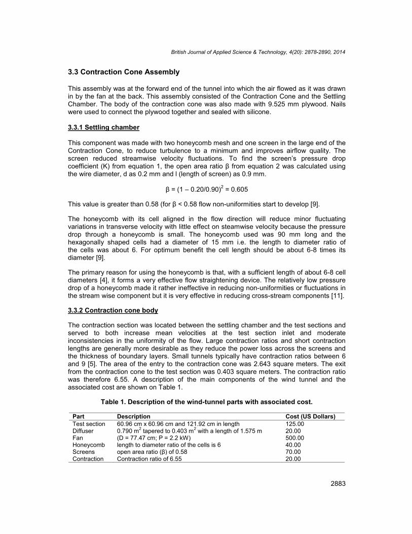
3.3 Contraction Cone Assembly

This assembly was at the forward end of the tunnel into which the air flowed as it was drawnin by the fan at the back. This assembly consisted of the Contraction Cone and the SettlingChamber. The body of the contraction cone was also made with 9.525 mm plywood. Nailswere used to connect the plywood together and sealed with silicone.

3.3.1 Settling chamber

This component was made with two honeycomb mesh and one screen in the large end of theContraction Cone, to reduce turbulence to a minimum and improves airflow quality. Thescreen reduced streamwise velocity fluctuations. To find the screen’s pressure dropcoefficient (K) from equation 1, the open area ratio β from equation 2 was calculated usingthe wire diameter, d as 0.2 mm and l (length of screen) as 0.9 mm.

β = (1 – 0.20/0.90)2 = 0.605

This value is greater than 0.58 (for β < 0.58 flow non-uniformities start to develop [9].

The honeycomb with its cell aligned in the flow direction will reduce minor fluctuatingvariations in transverse velocity with little effect on steamwise velocity because the pressuredrop through a honeycomb is small. The honeycomb used was 90 mm long and thehexagonally shaped cells had a diameter of 15 mm i.e. the length to diameter ratio ofthe cells was about 6. For optimum benefit the cell length should be about 6-8 times itsdiameter [9].

The primary reason for using the honeycomb is that, with a sufficient length of about 6-8 celldiameters [4], it forms a very effective flow straightening device. The relatively low pressuredrop of a honeycomb made it rather ineffective in reducing non-uniformities or fluctuations inthe stream wise component but it is very effective in reducing cross-stream components [11].

3.3.2 Contraction cone body

The contraction section was located between the settling chamber and the test sections andserved to both increase mean velocities at the test section inlet and moderateinconsistencies in the uniformity of the flow. Large contraction ratios and short contractionlengths are generally more desirable as they reduce the power loss across the screens andthe thickness of boundary layers. Small tunnels typically have contraction ratios between 6and 9 [5]. The area of the entry to the contraction cone was 2.643 square meters. The exitfrom the contraction cone to the test section was 0.403 square meters. The contraction ratiowas therefore 6.55. A description of the main components of the wind tunnel and theassociated cost are shown on Table 1.

Table 1. Description of the wind-tunnel parts with associated cost.

Part Description Cost (US Dollars)Test section 60.96 cm x 60.96 cm and 121.92 cm in length 125.00Diffuser 0.790 m2 tapered to 0.403 m2 with a length of 1.575 m 20.00Fan (D = 77.47 cm; P = 2.2 kW) 500.00Honeycomb length to diameter ratio of the cells is 6 40.00Screens open area ratio (β) of 0.58 70.00Contraction Contraction ratio of 6.55 20.00


2884

4. CALIBRATION OF THE WIND TUNNEL

Experimental measurements were conducted to calibrate the laboratory built wind tunnel.Wind speed through the tunnel was controlled by a variable speed WEG 3.00 hp motor driveunit with a WEG CFW 08 vector inverter plus motor speed control unit. Calibrationmeasurements included the boundary layer velocity profile and the wind velocity versesinches of water expressed in terms of milliamps, in the working section, in terms of thedifferential pressure values in the contraction cone. Calibration tests were performed using ahot-wire anemometer to determine the wind velocity as a function of differential pressuremeasured using a pressure transducer

4.1 Anemometer Selection

The hotwire anemometer used was the Amprobe TMA20HW. The Amprobe TMA20HW HotWire anemometer technology eliminates the use of bearings and rotating parts. The meter isdurable and provides good and stable accuracy of the measurements. This is a highlyaccurate anemometer with 0.1% basic accuracy for precise measurements with an air flowmeasurements range of 0.3 m/s to 30.0 m/s. The electrical specifications of the AmprobeTMA20HW anemometer are listed below in Table 2.

Table 2. Electrical specifications of the Amprobe anemometer

Feature Range AccuracyAir Flow 0.1 to 30 m/s ±3% of reading

0.2 to 110 km/hr10 to 6000 ft/min0.1 to 59 knots0.12 to 68 MPH

±1% FS

Air flow Volume 0.0 to 9999 CFM ±1% FSTemperature -20oC to 60oC ±0.5oC

-4 F to 140 F ±0.9 FHumidity 0.0 to 100 % ±3% RH

4.2 Differential Pressure Sensor Selection

In order to determine the right pressure sensor for the wind tunnel, preliminary testsmeasured the pressure range for its location. This was done using the wind speed atdifferent locations in the wind tunnel. Experiments performed in the Open Wind Tunnel with ahot wire anemometer showed that the velocity ranged between 3 m/s to 16 m/s. This wasrelated to the dynamic pressure by using Bernoulli’s Equation:= + (3)

This equation ignored the effects of compressibility, which was a good assumption for lowspeed flows. To find how this relates to the tunnel measuring system, or inches of a watercolumn, equation 4 was used.

P = ρgh (4)


2885

The unit used to measure the pressure difference was inches of a water column. To find outthe largest pressures a combination of equations 3 and 4 was used. The dynamic pressure inBernoulli’s equation can be set equal to the dynamic pressure in equation 4.= ℎ (5)

To determine the height of the water column equation 6 can be used.ℎ = (6)

Substituting ρair – 1.145 kg/m3, V – 16 m/s, ρwater – 995 kg/m3, g – 9.806 m/s2.

This gave a value of 0.015 m, which is 0.592 inches.

Using this data, the Setra Model M264 Differential Pressure Transmitter was selected for thiswind tunnel. This low-air pressure transmitter capable of sensing differential pressure in bothnegative and positive ranges. The Model M264 incorporates a tensioned stainless steeldiaphragm to form a variable capacitor that will produce variation in the output signal (4mA to20mA). It’s specifications are listed below in Table 3.

Table 3. Specifications of the Setra Model M264 Differential Pressure [12]

Specifications SpecificationsSupply Voltage 9 to 33 VDC Operating Temp -18ºC to 79ºCSignal Output 4 – 20 mA (two wire);

Voltage 0 – 5 VDC(three wire)

AdditionalspecificationRangeUp to 0.5” WCUp to 1.0” WCUp to 2.5” WCUp to 5.0” WC

Unit is factorycalibrated at 0gZero offset (%FC/g)0.060.050.220.14

Accuracy ±1% FS, RSS (atconstant temp)0.1% FS Hysteresis0.2%FS

Maximum OutputImpedance mA

800Ώ @24 VDC ProcessConnection

3/16” OD barbedbrass

Minimum OutputImpedance VDC

≥ 5000 Ώ Enclosure rating Glass-filled polyesterTemp range 0to150 F(-18to65ºC)

Repeatability 0.05% FS Approvals CEThermal Effect Compensated

temperature range 0to 150 F (-18 to65ºC) Zero/Spanshift o.033 F(0.018ºC)

Overpressure Up to 10 psig (68.95kPa) range dependant

Hysteresis ±0.1% FCDimensions 14x7.62x4.85 cm

Weight 0.55 lb (0.25 kg) Warranty 3 years


2886

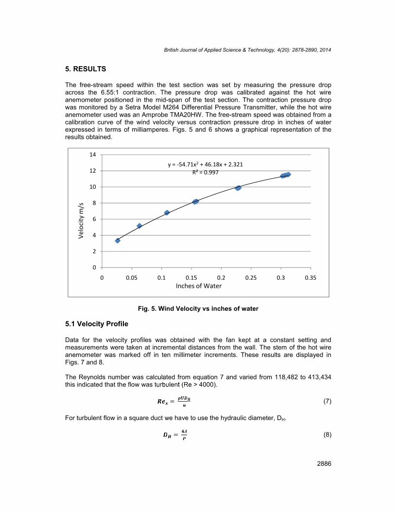
5. RESULTS

The free-stream speed within the test section was set by measuring the pressure dropacross the 6.55:1 contraction. The pressure drop was calibrated against the hot wireanemometer positioned in the mid-span of the test section. The contraction pressure dropwas monitored by a Setra Model M264 Differential Pressure Transmitter, while the hot wireanemometer used was an Amprobe TMA20HW. The free-stream speed was obtained from acalibration curve of the wind velocity versus contraction pressure drop in inches of waterexpressed in terms of milliamperes. Figs. 5 and 6 shows a graphical representation of theresults obtained.

Fig. 5. Wind Velocity vs inches of water

5.1 Velocity Profile

Data for the velocity profiles was obtained with the fan kept at a constant setting andmeasurements were taken at incremental distances from the wall. The stem of the hot wireanemometer was marked off in ten millimeter increments. These results are displayed inFigs. 7 and 8.

The Reynolds number was calculated from equation 7 and varied from 118,482 to 413,434this indicated that the flow was turbulent (Re > 4000).= (7)

For turbulent flow in a square duct we have to use the hydraulic diameter, DH.= (8)

y = -54.71x2 + 46.18x + 2.321R² = 0.997

0

2

4

6

8

10

12

14

0 0.05 0.1 0.15 0.2 0.25 0.3 0.35Inches of Water

Velo

city

m/s


2887

where A is the area and P is the wetted perimeter.

For turbulent flow in a square duct the shear is nearly constant along the sides, dropping offsharply to zero in the corners. This is because of the phenomenon of turbulent secondaryflows in which there are non-zero mean velocity, v and w in the plane of the cross-section.The Hydraulic diameter for this test section is 0.6096 m.

Fig. 6. Wind Velocity vs milliamps

Fig. 7. Wind velocity vs. wall distance

y = 0.088x2 + 0.146x + 3.749R² = 0.999

0

2

4

6

8

10

12

14

16

18

20

0 2 4 6 8 10 12 14

Velo

city

( m

/s)

mA

y = -0.000x2 + 0.015x + 4.346R² = 0.998

4

4.5

5

5.5

6

0 20 40 60 80 100

Velo

city

(m/s

)

Distance from wall (mm)


2888

Fig. 8. Wind velocity vs. wall distance

From documented data [14], b/a = 1. The effective diameter was calculated from equation 9.= . (9)

The effective diameter was 0.6855 m.

Equation 10 is the friction velocity.

∗ = /(10)

The velocity profile for turbulent flow was= ∗ ∗ + − (11)

where k is 0.41, B is 5.0 and h is the distance from the centre line to the wall of the testsection.

The roughness factor for Plexiglas [13,14], ε – 0.0015 mm.

Now ε/DH = 0.00000246. Using the Moody chart [15] the friction factors (f) were read off.Using equation 12.

∗ = ∗ /(12)

where the boundary layer separation is∗ = . / (13)

y = -0.000x2 + 0.053x + 9.048R² = 0.994

9

9.5

10

10.5

11

11.5

12

0 20 40 60 80 100

Velo

city

(m/s

)



2889

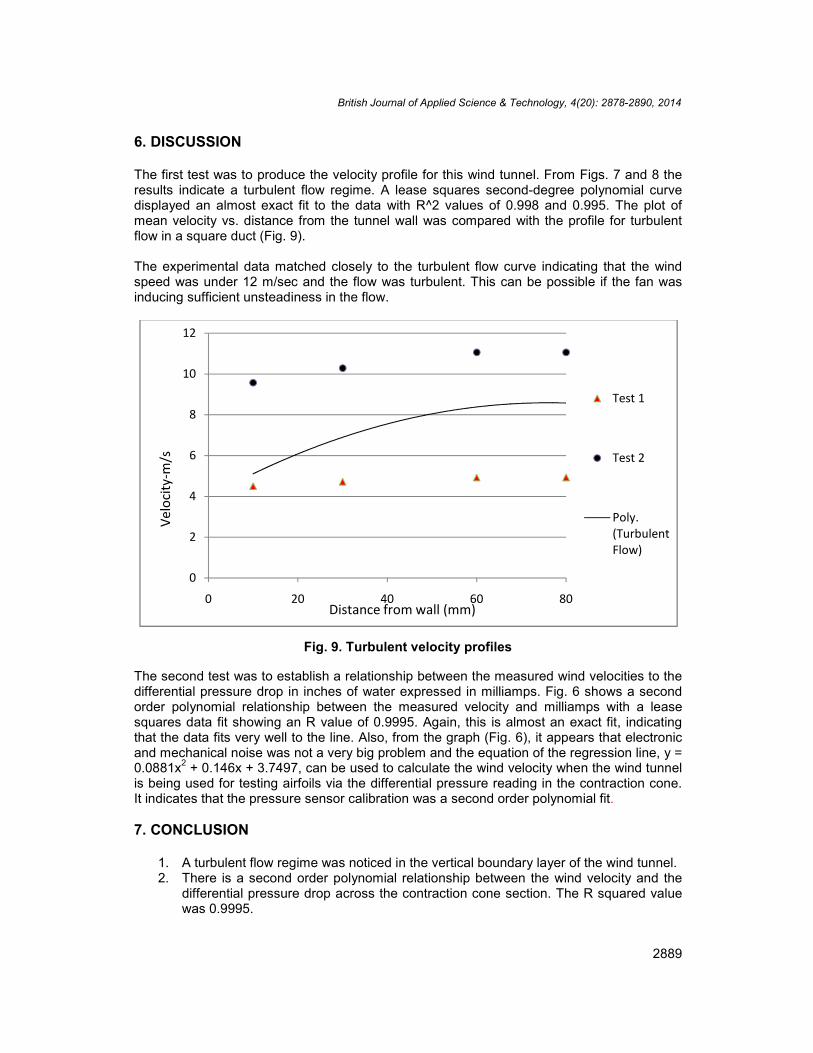
6. DISCUSSION

The first test was to produce the velocity profile for this wind tunnel. From Figs. 7 and 8 theresults indicate a turbulent flow regime. A lease squares second-degree polynomial curvedisplayed an almost exact fit to the data with R^2 values of 0.998 and 0.995. The plot ofmean velocity vs. distance from the tunnel wall was compared with the profile for turbulentflow in a square duct (Fig. 9).

The experimental data matched closely to the turbulent flow curve indicating that the windspeed was under 12 m/sec and the flow was turbulent. This can be possible if the fan wasinducing sufficient unsteadiness in the flow.

Fig. 9. Turbulent velocity profiles

The second test was to establish a relationship between the measured wind velocities to thedifferential pressure drop in inches of water expressed in milliamps. Fig. 6 shows a secondorder polynomial relationship between the measured velocity and milliamps with a leasesquares data fit showing an R value of 0.9995. Again, this is almost an exact fit, indicatingthat the data fits very well to the line. Also, from the graph (Fig. 6), it appears that electronicand mechanical noise was not a very big problem and the equation of the regression line, y =0.0881x2 + 0.146x + 3.7497, can be used to calculate the wind velocity when the wind tunnelis being used for testing airfoils via the differential pressure reading in the contraction cone.It indicates that the pressure sensor calibration was a second order polynomial fit.

7. CONCLUSION

1. A turbulent flow regime was noticed in the vertical boundary layer of the wind tunnel.2. There is a second order polynomial relationship between the wind velocity and the

differential pressure drop across the contraction cone section. The R squared valuewas 0.9995.

0

2

4

6

8

10

12

0 20 40 60 80

Test 1

Test 2

Poly.(TurbulentFlow)

Velo

city

-m/s



2890

3. Electronic and mechanical noise was not a affecting the differential pressuretransducer output.

4. The equation derived from the plot of wind velocity vs. milliamps (inches of water)can be used to calculate the wind velocity when the wind tunnel is to be used fortesting airfoils. (Wind speed through the tunnel was controlled by a variable speedWEG 3.00 hp motor drive unit with a WEG CFW 08 vector inverter plus motor speedcontrol unit).

5. The total cost was $ 775.00 US dollars.

COMPETING INTERESTS

Authors have declared that no competing interests exist.

REFERENCES

1. Pope A. Low-Speed Wind Tunnel Testing. John Wiley and Sons, New York; 1966.2. Tavoularis, Stavros. Measurement in Fluid Mechanics, Cambridge University Press;

2005.3. Rae WH, Pope A. Low-speed wind tunnel testing. 2nd edition. John Wiley & sons;

1984.4. Bradshaw P, Pankhurst RC. The design of low-speed wind tunnels. Progress in

Aeronautical Sciences. 1964;6:1-69.5. Mehta RD, Bradshaw P. Design Rules for Small Low Speed Wind Tunnels.

Aeronautical Journal. 1979;443-449.6. Morel T. Comprehensive Design of Axisymmetric Wind Tunnel Contractions. ASME

Journal of Fluids Engineering. 1975;225-233.7. Ramaseshan S, Ramaswamy MA. A Rational Method to Choose Optimum Design for

Two-Dimensional Contractions. ASME Journal of Fluids Engineering. 2002;124:544-546.

8. Wieghardt. On the Resistance of Screens, Aero. Quarterly, Royal Aero Society.1953;4.

9. Bradshaw P, Mehta R. Wind Tunnel Design; 2003.Available: http://www.htglstanford.edu/ bradshaw/tunnel/wadiffuser.html

10. Cockrell DJ, Markland E. Diffuser behavior, a review of past experimental work,relevant today. Aircr Engng.1974;46:16.

11. Scheiman J, Brooks JD. Comparison of experimental and theoretical turbulencereduction from screens, honeycomb and honeycomb-screen combinations. JAS.1981;18:638-643.

12. Available: www.setra.com/.../Pressure/Differential-Pressure/Air.../264-Data-Sheet.as13. Moody LF. Friction factors for Pipe Flow. ASME Trans. 1944;66:671-684.14. White MF. Fluid Mechanics. McGraw-Hill Inc, New York. 1994;333.__________________________________________________________________________© 2014 Ramkissoon and Manohar; This is an Open Access article distributed under the terms of the CreativeCommons Attribution License (http://creativecommons.org/licenses/by/3.0), which permits unrestricted use,distribution, and reproduction in any medium, provided the original work is properly cited.

Peer-review history:The peer review history for this paper can be accessed here:

http://www.sciencedomain.org/review-history.php?iid=537&id=5&aid=4654

design and calibration of a low speed wind tunnel · british journal of applied science &...

Documents