demand based tactical planning of the roundwood supply …
TRANSCRIPT

DEMAND BASED TACTICAL PLANNING OF THE ROUNDWOOD SUPPLY CHAIN WITH RESPECT TO
STOCHASTIC DISTURBANCES
Daniel Hultqvist, Mid Sweden University Leif Olsson, Mid Sweden University
Rapportserie FSCN – ISSN 1650-5387 2003:19 FSCN rapport R-03-44
April, 2004
Mid Sweden University Fibre Science and Communication Network SE-851 70 Sundsvall, Sweden Internet: http://www.mh.se/fscn


FSCN/System Analysis and Mathematical Modeling Internet: Http/www.mh.se/fscn
R-03-44 Page 2 (58)
INNEHÅLLSFÖRTECKNING Abstract............................................................................................................................. 3 1. Introduction .................................................................................................................. 4
1.1 Outline of the paper ................................................................................................ 5 2. Description of the roundwood supply chain................................................................. 5
2.1 Overview of the roundwood supply chain.............................................................. 5 2.2 Harvesting, forwarding and small forest owners.................................................... 7
2.2.1 Harvesting the own forest................................................................................ 7 2.2.2 Small forest owners ......................................................................................... 8
2.3 Roundwood transportation and roads..................................................................... 9 2.4 Roundwood storage .............................................................................................. 11 2.5 Roundwood markets and swapping of roundwood .............................................. 13 2.6 The demand problem at the mills ......................................................................... 15 2.7 A sample problem................................................................................................. 17 2.8 A real world problem............................................................................................ 18
3. Uncertainty ................................................................................................................. 19 3.1 Probabilities.......................................................................................................... 19 3.2 Uncertainty measures ........................................................................................... 20
4. The mixed integer quadratic model ............................................................................ 21 4.1 Explanation of the model...................................................................................... 21
4.1.1 The objective function................................................................................... 21 4.1.2 The constraints............................................................................................... 22
4.2 Modelling ............................................................................................................. 25 4.2.1 Scenario properties ........................................................................................ 27 4.2.2 Non-considered aspects ................................................................................. 27
5. Result from modelling ................................................................................................ 29 5.1 The sample problem ............................................................................................. 29 5.2 Solving a real world problem ............................................................................... 30 5.3 Value of the uncertainty measures ....................................................................... 31
6. Discussion and concluding remarks ........................................................................... 32 6.1 The sample problem ............................................................................................. 32 6.2 The real world case problem ................................................................................ 33 6.3 Do we need a stochastic model?........................................................................... 33 6.4 Future extensions.................................................................................................. 34
7. Acknowledgements .................................................................................................... 34 APPENDIX A: optimization model ............................................................................... 35
A.1 Mathematical formulation ................................................................................... 35 A.1.1 The objective function .................................................................................. 35 A.1.2 The constraints.............................................................................................. 36
A.2 Definitions ........................................................................................................... 40 A.2.1 Sets................................................................................................................ 40 A.2.2 Parameters .................................................................................................... 40 A.2.3 Costs ............................................................................................................. 42 A.2.4 Variables....................................................................................................... 43
Appendix B: Estimation of costs .................................................................................... 45 B1: Harvest costs from the own forest ........................................................................... 45 B2: Transportation costs................................................................................................. 47 B3: Roundwood storage costs ........................................................................................ 47 B4: Total cost for import and domestic roundwood....................................................... 51 Appendix C: Optimal rotation time for safety stock ...................................................... 52

FSCN/System Analysis and Mathematical Modeling Internet: Http/www.mh.se/fscn R-03-44 Page 3 (58)
DEMAND BASED TACTICAL PLANNING OF THE ROUNDWOOD SUPPLY CHAIN WITH RESPECT TO STOCHASTIC DISTURBANCES Daniel Hultqvist and Leif Olsson Mid Sweden University, Sundsvall, Sweden ABSTRACT
There are usually many sources for the supply of raw material to a pulp or paper mill in Sweden. The decision-maker can procure raw material from the company’s own forest(s), buy in from the owners of small forests, swap with other forest operators or purchase on the international market. Wood chips for these mills are brought from sawmills and have their own transportation system, but are included in the model presented here. Optimizing the supply of raw material at a tactical planning level is a challenging task, and can only be managed properly if elements of uncertainty are considered. The solution would otherwise give few options when disturbances occur, for example when weather conditions change. The deterministic equivalent of the stochastic scenario model is formulated and solved as a convex mixed integer quadratic model. The model is tested on one small sample problem and one full-scale problem. We show how to simulate and evaluate different strategies in the flow of raw materials, from harvesting operations to delivery at the mills. In our study, the full-scale problem has been solved within reasonable time using commercially available software, and the solution indicates that the hedging effect in the stochastic solution adds flexibility. Keywords: Mixed-Integer Quadratic Programming, Forest Logistics, Scenario Modelling, Uncertainty, Roundwood Storage, Forest Roads, Roundwood market, Flexibility.

FSCN/System Analysis and Mathematical Modeling Internet: Http/www.mh.se/fscn
R-03-44 Page 4 (58)
1. INTRODUCTION In recent years the forest companies in Sweden have moved their focus from
harvest decisions, which have been relatively well investigated, to forest logistics, road investments (Olsson 2004a, Olsson 2004b, Olsson 2004c, Arvidsson et al. 2000) and storage of roundwood after harvesting (Persson et al. 2002a, Persson & Elowsson 2001, Liukko & Elowsson 1999). None of these questions have been accurately answered, although case studies indicate that optimal road investments can be calculated in an efficient manner, as in Olsson (2004a, 2004b, 2004c). The Forest Research Institute of Sweden (SkogForsk) are now in the progress of developing a decision support system for planning of road investments.
As opposed to road investments, there are no definitive figures for the cost of roundwood storage. Although studies exist, as in Persson et al. (2002a), Persson & Elowsson (2001), Arvidsson & Holmgren (1999) and Liukko & Elowsson (1999), it is in general very hard to estimate the cost of value losses and how roundwood of low quality affect the pulp and paper process at different mills. The problem will differ with assortment, weather, time of year and industry process, as well as storage location etc. Hence, a lot of the parameters are affected by the uncertainty and chaos of the real world (Prigogine & Stengers 1984). Hence, in general they are very hard to predict. Furthermore, we can’t assume that the decisions in harvesting, transport and forest industry are independent, since decisions have to be flexible, as put forward by Barros & Weintraub (1982) and Weintraub & Navon (1976). Hence, we have to optimize the whole roundwood supply chain to get an optimal solution. There are also studies that indicate substantial gains if we integrate the process at the mills with roundwood supply chain planning (Arlinger et al. 2000, Berg et al. 1995b).
Here we describe and test a network design model (Cranic 1998, Coudeau et al. 2003) that integrates different aspects of the raw material supply chain from harvesting to industrial processing that still can be solved within a reasonable time frame. The model focuses on procurement of raw material from forest owned by the mill. We have, however, included the purchase of roundwood on the domestic and international market in the model as well as swapping between companies.
In contrast to other attempts to optimize the raw material supply with purely deterministic models as in, for example Karlsson (2002) and Bredström et al. (2001), our stochastic model focuses on procurement with respect to uncertain load-bearing capacity of roads and harvesting grounds. Further, seasonal roundwood price trends estimated from historical data (Skogsvårdsorganisationen) are also incorporated in the model. However, prices are not assumed to be stochastic processes (Hjort 1996), as in for instance Gong (1998) or Lohmander (1999).
We develop a scenario optimization model (Birge & Louveaux 1997, Kall & Wallace 1994) that can be represented as a minimum cost network flow model (Rardin 1998) with dynamic information constraints (Lohmander & Olsson 2004). The deterministic equivalent of the scenario model is formulated and solved as a convex mixed integer quadratic model (Wolsey 1997). The reason why to use a scenario model is motivated with the Value of the Stochastic Solution (VSS), and the Expected Value of Perfect Information (EVPI), that describes the difference between the solution under uncertainty and certainty. Someone may argue that it is only to use what-if analysis instead of a scenario optimization model. However, this is in general not true, as well described in Wallace (2000). Even in the cases where it is enough to use deterministic

FSCN/System Analysis and Mathematical Modeling Internet: Http/www.mh.se/fscn
R-03-44 Page 5 (58)
models and use what-if analysis, one has to solve the stochastic version of the model first. Only when it has been solved can one, by means of VSS, see if the deterministic solution will be accurately enough for this instance of the problem (Wallace 2003). Uncertainty measures are further described in Birge & Louveaux (1997), and in section 3.5.
We describe the features of the model with a sample problem and show that it is possible to solve a full-scaled problem with commercial software (Anon. 2002) and a standard PC, without using any decomposition technique, in reasonable time, with a adequately amount of scenarios and time periods. This is an interesting result since most people usually assume that it is impossible to incorporate randomness in large scaled optimization problems. However, we show in this paper that this is not always the case anymore. Furthermore, our intention is to decompose the scenario optimization model and solve with parallel processors in the future. Useful decomposition algorithms already exist for this type of problem as described, in for instance, Linderoth & Wright (2003) and give us the possibility to include more uncertainty and time periods in a future model, and still solve the problem in reasonable time. 1.1 Outline of the paper
We start with the description of the roundwood supply chain problem and assumptions in the next section. In section three probabilities and uncertainty measures. In section four, we present the mixed integer quadratic model in words.
In section five, we present results from the optimization of a sample example, as well as some results from a full-scaled problem. The last section contains the discussion and concluding remarks. In the appendix A the mathematical model with explanation of the notation are presented. In appendix b the costs used in the optimization are accounted for and appendix C a description of the optimal replacement time for safety stock of roundwood. 2. DESCRIPTION OF THE ROUNDWOOD SUPPLY CHAIN The rules and regulations surrounding the forest industry vary from country to country. We will therefore give an overview of how a pulp or paper mill in Sweden is procured. This will include the whole supply chain and also put it into different perspectives. That is from both the mill and, since a large proportion of the Swedish woods is owned by persons only owning a few hectares, from a small forest owner’s view. 2.1 Overview of the roundwood supply chain
We begin with an overview of our roundwood supply chain problem. We intend to include all essential aspects in the scenario model and to solve it on an annual basis. Motivations are stated in detail in the following subsections, and the problem, described below, is depicted in Figure 2.

FSCN/System Analysis and Mathematical Modeling Internet: Http/www.mh.se/fscn
R-03-44 Page 6 (58)
• First step is to harvest the trees with the harvester and put the trees in log piles. • Then, we pick up the log piles with a forwarder and transport to roadside.
However, here we assume no costs are related to roundwood storage in the forest, since good planning will decrease forest storage to a low level. This is also an independent optimization problem, which can be solved without taking the rest of the supply chain into account.
• Observe that instead of these two machines we can sometimes use a combined machine called a harwarder (Figure 1), or buy roundwood from small forest owners directly at roadside.
• Then the log piles located roadside are put on a truck or stored there if it can’t be transported on the road.
• If possible, we haul the roundwood on the roads to a terminal storage, a better road or directly to the mills.
• If it is not possible to use a sufficient amount of roads to secure the roundwood demand at the mills, we have to purchase wood at some external market, transport roundwood from the security stock or in advance move the roundwood to an accessible road for further transport to the mills. This is a very common strategy during the spring thaw.
• Infrastructure investments are not included as an option in the model since these are long-term decisions as described in Olsson (2004a, 2004b, 2004c).
• The model can handle railway transportations, even if it is not included in Figure 2.
Figure 1: A harwarder in a Swedish forest. Experiments show that this single machine can compete economically with a two machine system. Not only in thinning operations but also in clear cutting (Hallonborg & Nordén 2000).
The description above is of course simplified to get the overall picture, and more
details are given in following subsections. However, one essential part in the model is that the road transportation of the roundwood is affected by the load-bearing capacity of the roads, as described by Hossein (1999) and Löfroth et al. (1992). The load-bearing capacity of the harvest areas also has to be taken into account. Further, load-bearing

FSCN/System Analysis and Mathematical Modeling Internet: Http/www.mh.se/fscn
R-03-44 Page 7 (58)
capacity, both on roads and on harvest ground, depends on weather conditions and are hence uncertain. In the model presented here we use a scenario optimization approach to incorporate uncertain load-bearing capacity in the model. This is further described in section 2.3 and for roads also in Lohmander & Olsson (2004).
Figure 2: An overview of the roundwood supply chain from forest to mill. Unfilled arrows indicate that hauling may be uncertain under some periods during a year. This uncertainty is handled with scenarios in the optimization model. 2.2 Harvesting, forwarding and small forest owners
In this section we will discuss roundwood supply in the area relatively close to the mill. It can be divided into three parts.
1. Harvesting the own forest. 2. Harvesting stumpage purchased from small forest owners. 3. Roundwood delivered by small forest owners directly to roadside.
The last two parts will be described together in section 2.2.2 since they both are
related to how small forest owners handle their properties. 2.2.1 Harvesting the own forest
Studies, as in for instance Arvidsson et al. (2000) and Carlsson et al. (1998) indicate that extraction of logs can be optimized. This is not included in our model. We

FSCN/System Analysis and Mathematical Modeling Internet: Http/www.mh.se/fscn
R-03-44 Page 8 (58)
assume that the extraction is optimized. This and the fact that harvester and forwarder are working in teams makes the harvesting cost more or less independent of this aspect.
We assume that the roundwood will not be stored as log piles in the forest. Unfortunately, that is usually not the case. However, when storage in the forest occurs, it should only be for a very short period of time, at least with good planning. This storage will then only have a minor affect on the roundwood in general, and can therefore be skipped completely.
A new type of machine has also been tested by the industry that is a combined harvester and forwarder, called a harwarder (Figure 1). If this machine is used, there will be no storage at all in the forest. Hence, to make the modelling easier, we assume that storage in the forest never occurs. We also divide harvesting in two different types.
1. Thinning. 2. Clear cutting.
Some machine groups can only handle one of these activities, others both. We have
assumed that we only use machine groups capable of performing both tasks. Even if this weren’t the case, when planning for a real case-problem, one will probably need more than one machine group. Probably it will be a lot more, at least for the larger industries. Therefore it will be no problem with machine groups that are only capable of performing one of these tasks. There will be several harvest sites to choose from, making it possible to schedule all machines according to their capacities. That is given that the mixture of pure thinning, pure clear cutting and machine groups able to performing both tasks are well designed. However, deciding this mixture is a strategic problem and is therefore not considered here. All machine groups used have been given the same capacity. By capacity we mean the capacity for the harvester, since the forwarders always are assumed to have a capacity that is equal to, or greater, than the harvester they are working together with. The capacity for clear cutting differs from the one for thinning. This is because thinning operations, where not all trees are cut, take longer time, as well as produces a smaller volume of roundwood since the trees themselves are younger, and hence smaller. 2.2.2 Small forest owners
Small forest owners mostly deliver their roundwood to the roadside or sell it on
the stumpage market, as put forward by Rylander (2000). The areas they sell as stumpage is handled as a part of the company’s own forest with an additional cost for the stumpage price. If the forest owner himself harvests the wood and delivers to a mill or roadside, this is seen as an external source. A fixed part of this volume will be billed an average cost for transportation to represent the volume that the forest company has to transport itself. With this approach small forest owners will be an endogenous part of our model. However, the optimization in our model is performed from a mill owner’s view, and not from the small forest owner’s point of view.
Small forest owners usually have other incomes as well (Bergman 1998). Hence, it is very important to decide the right price level for companies buying from these owners. Furthermore, most of these owners want to deliver their roundwood during the

FSCN/System Analysis and Mathematical Modeling Internet: Http/www.mh.se/fscn
R-03-44 Page 9 (58)
winter or spring (Anon. 1999b), if at all, since they usually do not need the money right a way.
One more thing is that small forest owners are to a higher extent dependent on the weather, as for instance, wind throwing highly affect their forest. However, these aspects haven’t been included in our model. More information how to optimize this subject can be found in, for instance, part three of Lohmander (1987).
The oligopsonized market situation is also an example where using random variables to reflect the behaviour of the market participants can be very dangerous, as shown by Haugen & Wallace (manus), using simple game theoretic models. 2.3 Roundwood transportation and roads
Roundwood is mostly hauled on roads from the forest to the mills. Hence, hauling is highly dependent of the roads. Unfortunately, during the thawing period in the spring and rainy periods, usually in the fall, the load-bearing capacity is very limited on most of the gravel roads (Hossein 1999, Olsson & Lohmander 2004). Hence, heavy loads can only be hauled on some roads of high quality during these periods.
Since our model is made for a tactical planning horizon, accurate infrastructure decisions such as upgrading of roads, and construction of new roads (Bergström 2001) should not be included. They are better made with a longer planning horizon, as motivated in Olsson (2004a, 2004b) and Olsson & Lohmander (2004). However, road maintenance can, and should, be included. They are divided into two parts:
• Fixed initial cost. Cost for eventually restoring roads, so that the harvest
site can be reached. Also includes some costs for preparing for the harvesting crew and areas to store harvested roundwood on.
• Volume dependent costs. This could be cost for maintaining the roads to sites with harvest operations, and also for the cost of snow removal during the winter season.
The first type of costs is included in the fixed cost for opening a harvest site.
The other one is added to the cost of transportation on the roads in question. These costs are highly dependent on the weather (Hossein 1999). Hence, we use scenarios to cope with uncertain weather conditions, as depicted in Figure 4.

FSCN/System Analysis and Mathematical Modeling Internet: Http/www.mh.se/fscn
R-03-44 Page 10 (58)
Figure 3: The scenario tree of our optimization model represent different outcomes of the stochastic variables.
In the scenario tree in Figure 3, we have following definitions.
• LOW = Low water content in the ground, keeping more roads and harvest areas
open. • MED = Normal water content in the ground, keeping a normal number of roads
and harvest areas open. • HIGH = High water content in the ground, causing more roads to be closed and
making more harvest areas than usual unavailable.
The load-bearing limitation on the roads is incorporated as a constraint in the optimization model, and is further described in section 4.2. Further, it is possible to close some roads during critical periods, if necessary. Table 1: Times when the roads of different classes are open or closed. The meaning of the notation for different scenarios is described above. Approximation of the roads states based on Lohmander & Olsson 2004.
Road class
Winter Spring LOW
Spring MED
Spring HIGH
Summer LOW
Summer MED
Summer HIGH
A Open Open Open Open Open Open Open B Open Open Open Closed Open Open Open C Open Open Closed Closed Open Open Closed D Open Closed Closed Closed Open Closed Closed
We want describe any more about roads here. However, gravel roads are very important for the hauling of roundwood and the interested reader find further information about this topic in Hossein (1999), Löfroth et al. (1992) and Olsson & Lohmander (2004). Surface roads are usually possible to use the whole year, as assumed in our study. Costs for transportation and maintenance of roads are found in Appendix A.2.
FSCN/System Analysis and Mathematical Modeling Internet: Http/www.mh.se/fscn
R-03-44 Page 11 (58)
We have some other restrictions about the roundwood transportation.
• The demand of roundwood is fixed • We do not include backhauling in the model
These assumptions are probably not too restrictive in general, since in most
cases the destination is already decided on our planning horizon, although some savings could be made with a non-fixed destination (Bergdahl 2002) and backhauling can only be used in some areas. In the northern part of Sweden almost all mills are located by the eastern coast. There are studies made in this part of the country showing that there exists some, but not many, possibilities for backhauling (Forsgren 1993). Furthermore, include backhauling in our model will dramatically decrease the possibility to solve large scaled problem instances (Carlgren et al. 2000, Carlsson & Rönnqvist 2001), and it can probably be solved separately on an operational level, without loss of generality, to generate transportation costs to our model. 2.4 Roundwood storage
The most challenging part of the roundwood supply chain is probably roundwood storage, and the following questions. 1. How does storage affect the quality of roundwood? 2. How does low or mixed quality of the roundwood affect the processes at the mills? 3. What is the cost of quality losses? 4. How much roundwood should be in storage?
Many have tried to answer these questions, as for instance Forsberg (2000), Hägg (1991), Persson et al. (2002a) and Persson & Elowsson (2001). Unfortunately, the answer is substantially different depending on a lot of things (Berg et al. 1995b), some of them listed below.
• Assortment • Weather and season • Weather and season when the roundwood was cut • Industry process • Storage time • Storage location • Sprinkling
Some other difficulties for the modelling are that roundwood log piles can be
stored very different. That is, some log piles will be stored one period, some two periods and some even longer, as depicted in Figure 4. This is the case since storage costs are not only dependent on time. As an example, log piles that are frozen during the winter manage storage in spring better then log piles of springwood, due to lower mould probability etc. (Sjöblom 2003, Skutin & Arvidsson 2000).
There are several negative effects of storing roundwood for a long time. This roundwood will suffer from higher wood looses in the debarking process. It will also

FSCN/System Analysis and Mathematical Modeling Internet: Http/www.mh.se/fscn
R-03-44 Page 12 (58)
contain less of bi-products like turpentine. The density of the wood will also diminish, since roundwood are paid for by volume this will lead to that the cost of production increases. Also the quality of the end product will suffer. More on how these aspects interacts with the economy of the mill can be found in Andersson (2001).
The time dependency of the storage constraints depicted in Figure 4 make it impossible to separate these constraints in different blocks as recommended in Birge & Louveaux (1997). These types of constraints are called dynamic information constraints and are described in Lohmander & Olsson (2004).
Scenarios also add to the complexity of the situation. Roundwood can initially be stored in every ancestor scenarios to the present one, as depicted in Figure 5. This increases the number of separated storage volumes with respect to the number of time periods in the tree.
The most challenging part is, however, the storage cost itself. The estimation used in our optimization is described in Appendix A.3. Nevertheless, further research is necessary to enable better approximations of these costs.
A study by Persson & Elowsson (2001) indicates that spruce pulpwood can dry rapidly when stored at roadside during summer conditions. Hence, in that case, the best policy is to store spruce pulpwood under sprinkling at terminal, however this is not always possible. The situation can however be different for different assortments and locations.
Figure 4: Roundwood flow at a typical storage node in the network. Observe that roundwood stored in period t can be used in all descendant periods. This is modelled as roundwood flow in time at the same storage location.

FSCN/System Analysis and Mathematical Modeling Internet: Http/www.mh.se/fscn
R-03-44 Page 13 (58)
Figure 5: Roundwood is sent from all ancestor scenarios to the previous one. We call it dynamic information constraints.
The last question, how much roundwood should be in storage, is not easy to answer correctly. The answer will depend on several aspects such as:
• The storage cost for the mill. • The ability to quickly acquire roundwood from external sources. • The possibility of swift changes in the delivery from the company’s own forests. • To accurately foresee the future demand. • Have accurate information of harvested volumes and the volume stored in the
forest.
All these aspects and several others have to be considered to find out the size of the storage. Another aspect is the risk a company is willing to take, i.e. the chance to end up without any roundwood to supply the mill. No matter how large a storage one keeps, one can never be 100% sure to never run out of roundwood. There is always a risk of that happening. Koskinen (1991) states that a modern mill normally can operate properly with a storage corresponding to 5-7 days of production.
However in Koskinen (1991) it is also proposed that minimizing the storage should be a primary target for a pulp mill. Both Hägg (1991) and Person (2001) are of the opinion that the size of the roundwood storage should rather be optimized than minimized. This is probably closer to the truth since the focus should be on minimizing the total cost of the procurement of the mill. This is achieved by for instance, buying more from external sources when the price is low or by more efficient use of the internal harvesting equipment. The interested reader can find more on this topic in Hägg (1991). 2.5 Roundwood markets and swapping of roundwood
Swapping roundwood with other companies is considered as virtual links in the network model (Figure 4), between other company mills (k) and internal mills (i). The cost related to this link is the own company’s additional cost for swapping. This cost is assumed to only be the transportation cost. The harvesting cost for the roundwood that is being swapped is included in the total cost of harvesting. If there are additional costs,

FSCN/System Analysis and Mathematical Modeling Internet: Http/www.mh.se/fscn
R-03-44 Page 14 (58)
or gains, this can be added to, or subtracted from, the transportation cost on this arc in the network.
We divide external purchases of roundwood into the domestic roundwood market and the international roundwood market here. The network representations of the markets are depicted in Figure 7.
Figure 6: A network representation of the roundwood supply from different sources into an internal mill i.
Prices on the international roundwood market and the domestic market are
estimated from historical data provided by Skogvårdsorganisationerna (SVO), and are presented in Appendix A.4, as well as approximation of the total costs including the value losses described in Appendix A.3.
We have no intention to foresee the market price on roundwood, since we do not believe that its possible to predict any roundwood market, at least on our short-term yearly basis, due to many exogenous chaos parameters (Prigogine & Stengers 1984), for instance: political decisions, weather phenomena and psychological factors, as described in for instance Meyer et al. (2002). To convince the reader, price fluctuations for conifer wood during 1998-2001 are compared in the diagram depicted in Figure 8.
300320340360380400420440460
1 2 3 4 5 6 7 8 9 10 11 12
BARR1998BARR1999BARR2000BARR2001
Figure 7: Import price of conifer wood for every month during a year. Compared for 1998, 1999, 2000 and 2001 with data from SVO. Notice the non-correlated behaviour during the spring. Further, that price seems to be low in the summer and high in the winter.

FSCN/System Analysis and Mathematical Modeling Internet: Http/www.mh.se/fscn
R-03-44 Page 15 (58)
There has been a lot of research, in forest economy, where the market
roundwood prices have been modelled as stochastic processes (Hjorth 1996), for instance as a first order AR-process in Gong (1998) and Lohmander (1999). Later as a first order ARMA-process in McGough (2002). However, these approximations have been used on long-term basis, and we are rather convinced that this approach works better in the long run, then on annual basis, as in our case.
Due to the unpredictable nature of the roundwood market, we decide to use roundwood market prices from 2001 in our study, since other price and cost estimations also are from this time period.
In our study the most important aspects of the market price trend is that market prices seems to always be lowest in the summer and highest in the winter, independent of the year. If we take a look at historical data from SVO, the only “chaotic” period, with no price trend, seems to be the spring.
Since there are no apparent differences in the market prices depending on weather. The external market variables will be independent of the weather scenarios, depicted as the event tree in Figure 4. 2.6 The demand problem at the mills Some decades ago, the industries kept huge volumes of roundwood stored at terminals. There were several reasons for this. The sulphite industries wanted debarked roundwood that had been stored more than one year to handle the resin problem in the raw material. Common for all industries were the problem of procuring the mills. Back then, most of the roundwood was harvested by the land owner himself and the industries had very little control over the flow of roundwood (Anon. 1999b). Since nobody wanted to end up without roundwood, the industries bought everything they could and kept huge storages to be on the safe side. Of the 66 sulphite mills that once existed in Sweden, only five are left today (Ragnar, 2004) and this at the same time as the technology developed. During the 80s the mechanization of the harvesting operations gained speed. That led to that the control of the harvesting operations shifted over to the industry. The harvest machines harvest all year around and not only in the winter, as the forest owners preferred. This in its turn led to that the storages could be reduced, since the harvesting operations produced the volume that the industry asked for, in approximately the same speed as the industry used up the supply (Anon. 1999b).
Another aspect is that the demand for chlorine-free products grew. Earlier roundwood of bad quality could be bleached to be bright white, it was just a question of how much chlorine gas to use. This increased the requirements on the roundwoods freshness (Skutin & Arvidsson 2000). The economic down turn in the beginning of the 90s also forced some companies to drastically decrease their storages due to economical reasons (Lampe & Söderlund 2002). The trend today is that the industry is working hard to get fresher roundwood delivered to the mills. Freshness is sometimes defined as the time between harvesting and delivery (Berg et al. 1995a). There are examples of mills that have cut the time from harvest to delivery at the mill during the last half decade from 80 to 12-15 days (Lönner & Ershammar 2000). In their work to get fresher raw material some mill have

FSCN/System Analysis and Mathematical Modeling Internet: Http/www.mh.se/fscn
R-03-44 Page 16 (58)
reduced their storages to a tenth of what they were in the middle of the 80s (Anon. 1999b).
The amount of roundwood harvested by the land owners themselves have decreased. Still studies show that when this roundwood is delivered to the mills the brightness of the pulp decrease to levels that are not acceptable (Anon 1999a). To solve this problem the land owners has to mark their roundwood with which week it was harvested. It is then down graded to a cheaper assortment if it is too old. To classify the roundwood according to how long it has been stored does not always give an accurate picture of its quality. In reality it is the three characteristics: debarking ability, moisture level and brightness that are of interest. These properties doesn’t change at the same rate all year round, it is faster in the summer and slower in the winter (Berg et al. 1995a). Since the moisture level also affects, among other things, the debarking ability, it might be better to classify according to the moisture level instead. It can easily be measured with NIR, Near Infra Red light (Persson et al. 2002b). When roundwood is stored the humidity decreases in the wood as time goes by. If the weather is sunny and windy, the roundwood dries out faster. Hence is there a difference between roundwood stored in dry weather and that stored in rainy weather. The quality of the roundwood, when it is time to use it, will be dependent on the weather. Some roundwood might have to be downgraded to another assortment after storage. It is also important at which time it was put into the storage. To solve this, the volume stored during each time period has to be separated and not just be added to the volume stored earlier. This will give the opportunity to downgrade roundwood that has become too old or too dried out.
Figure 8: An example on downgrading of roundwood when stored from period 1 to period 4. Using more gradings of every assortment is a relevant way to model this. The straight arrows in the middle represent volumes stored in the previous time period. The bent dotted arcs on the right represent the volume originally stored during the first time period. The bent arc on the left, between the last two time periods, represents the volume originally stored in time period two. When using fresh roundwood the amount of chemicals used in the manufacturing process can be reduced. This in its turn leads to that the economical margins for the producer increases, which is good. Now the industry has started to look at other aspects that would decrease the productions costs. One way is to minimize the

FSCN/System Analysis and Mathematical Modeling Internet: Http/www.mh.se/fscn
R-03-44 Page 17 (58)
energy needed for the production. Studies show that if the roundwood has fibres more suitable for the products manufactured, the energy consumption decrease (Berg et al. 1995b). To consider the roundwoods fibre properties also opens up for other possibilities. The fibre properties of roundwood is correlated to the way the tree has grown, which part of the tree it is, if it is harvested in a thinning operation or in a clear cutting (Arlinger et al. 2000, Berg et al. 1995b). By taking advantage of this and using the right raw material for the product, not only might the production costs decrease, but the end product can also be given much better properties (Arlinger & Wilhelmsson 1998). Calculations from the forestry research institute of Sweden show that half a billion SEK could be saved in Sweden on an annual basis with this strategy (Arlinger & Wilhelmsson 1998). This is calculated for the production of cardboard alone. The assumption is that 20 percent of the total production would be able to save 6 percent of its raw material cost. In the south of Sweden, one mill sorts the incoming roundwood after its properties. The sorting is done at the same time as the volume is measured. Hence, the sorting is done on a truckload basis and there can still be large differences of the properties on the roundwood on a single truck. Still, the profit for the mill is estimated to 10 million SEK per year. This is more of an under estimate then an over estimate (Arlinger et al. 2000). Since the sorting at the mill is done at the same time as the volume measurement, the cost for this is very low. If the sorting would take place in the forest, the cost would increase. The capacity for the harvester goes down with 1 percent per assortment added. At the same time the capacity of the forwarder goes down with 3 to 4 percent per new assortment (Brunberg & Arlinger 2001). To take full advantage of the fibre properties the supply chain has to take a full step over to a pull flow. Earlier, when the industry had to make the best they could with what the forest owners harvested, it was a complete push flow. At present time the industry is somewhere in between, but probably, still closest to a push flow. The industry has to find out exactly what properties they want, how much and they must be willing to pay extra for this service. On the plus side, the mills will get better products to a lower cost. 2.7 A sample problem
When developing a model of a complicated and complex problem, there is a need for a sample problem. This problem should be small enough so that it is easy to get a feel of the meaning of the solution. Hence, it is easier to see if things don’t behave as they should. Since the model contains the whole supply chain even the smallest problem becomes quite large.
The artificial sample problem is depicted in figure 9. The problem includes harvest areas for the harvest planning part of the model and roads for the logistic parts of the model. There are both a saw mill and a pulp or paper mill included in the problem. Furthermore, there is also a joint storage terminal to handle the storage for both mills.

FSCN/System Analysis and Mathematical Modeling Internet: Http/www.mh.se/fscn
R-03-44 Page 18 (58)
Figure 9: A small sample problem with 18 possible harvest areas, 20 roads, one storage, one saw mill and one paper mill.
An important part of the model is the roads that have different classes, depending on the road-construction (Fig. 10). The paved roads are all a-class roads. The classes b through d are all different classes of gravel roads. Their accessibility is described in Table 1 and has been taken from Löfroth et al (2000).
Figure 10: The classifications for each of the 20 roads in the sample problem. Class a is paved roads and b trough d are unpaved roads where class b is the best.
2.8 A real world problem It is not enough to make a model that can handle sample problems, it must also be able to handle problems of a useful size. Therefore we tested the model on a real case from a mill, Iggesund, in the central of Sweden. This mill is a part of the forest company Holmen and produces virgin fibre paperboard. The company has large areas of forest to supply this mill. They administrate five forest districts, where four districts supply mainly this mill. One of these disctricts, the one named Sveg, became our selected problem area. This is a district covering, in total, approximately an area of 11,500 km2. Not all of this is owned by Holmen, but the company’s forest is scattered

FSCN/System Analysis and Mathematical Modeling Internet: Http/www.mh.se/fscn
R-03-44 Page 19 (58)
all over the whole district. It consists of approximately 320 harvest areas and 450 roads. The roads are a mixture of federally owned paved roads and roads owned by Holmen, other forest companies or private interests in the region.
Figure 10: The district Sveg owned by Holmen Skog in the central Sweden.
From this district the roundwood is transported east to the cost. Both the paper mill and the saw mill are located by the cost. 3. UNCERTAINTY 3.1 Probabilities
Except for the first period, representing the winter season where everything is frozen, we have three scenarios in time period two and three. Hence there will be one scenario in the first time period, three in the second and in the third period three scenarios for each one of the three scenarios in time period two. This will give a total of nine in the last time period, as depicted in Figure 4. An interesting question is:
• What is the probability that scenario k happens during period t?
The answer is that it depends on how we define wet, normal and dry weather. Hence, we assume that its equal likely that it will be dry, wet or normal weather conditions in our general model. However, applied in reality, the scenario distribution can be estimated from historical weather data, for any geographical area, and generated with for instance moment-matching scenario generation (Höyland et al. 2003). We also

FSCN/System Analysis and Mathematical Modeling Internet: Http/www.mh.se/fscn
R-03-44 Page 20 (58)
have to remember that a uniform distribution is a much better approximation of the reality then a distribution with all the mass in the mean, as in a deterministic model. Further, the important part is to include flexibility and options in our solutions. It is always possible to decide an arbitrary probability discrete function in a way that gives us a uniform distribution with respect to low, medium or high water content in the roads (Olsson 2004d).
We use a discreet uniform distribution (Blom 1984) in the rest of this paper. Hence in period two all probabilities are 1/3 and in period three 1/9, if we uses scenarios as in Figure 4. 3.2 Uncertainty measures
We use two types of uncertainty measures in the same way as described in Birge & Louveaux (1997). These measures are the Value of the Stochastic Solution (VSS) and the Expected Value of Perfect Information (EVPI). Another way to measure uncertainty is to use simulation. However, it is not used here, since uncertainty analysis is not the core part of this paper.
The VSS measures the value of including randomness. In economics, and especially real option theory (Wallace 2003; Amren & Kulatilaka 1999) the VSS is often called the option value or the value of flexibility. These are simply different names for the same uncertainty measure. It can be calculated in the following steps, as well described in Kall & Wallace (1994).
• Solve the mean value (EV) problem to get a first stage solution. • Fix the first stage solution and solve for all other second stage scenarios, with
the mean value scenarios in all other periods. • Fix the variables in scenario 2, and if we have only three scenarios, we solve the
problem for all scenarios with fixed variables in period one and two. • If we have more periods, it is only to repeat! • We call the solution from this nested calculation the expectation of the EV
solution or simply EEV. • Calculate the scenario model solution or stochastic programming solution called
SP. • The VSS is calculated as:
VSS = EEV-SP.
• VSS with the above definition is always greater then equal to zero, since the
stochastic solution (SP) always is less then or equal to the “worse” EEV solution in a minimisation.
The EVPI measures the cost of uncertainty and is calculated in following steps.
• Solve the deterministic problem for all of our scenarios. In our case with three periods we have nine scenarios, hence we have to solve nine problems.
• Calculate the mean value of this solution and we get the “wait and see solution” WS. This is the solution if we assume perfect knowledge about the future.

FSCN/System Analysis and Mathematical Modeling Internet: Http/www.mh.se/fscn
R-03-44 Page 21 (58)
• The EVPI is then in the minimisation case calculated as:
EVPI= SP-WS.
• EVPI is with the above definition also always greater then equal to zero, since the stochastic solution (SP), in a minimisation, always is greater then equal to the “better” wait and see solution (WS).
Calculating this uncertainty measures give us interesting information. A high
value on the VSS means that it is of substantial value to solve the scenario model, and maybe it will be valuable to include more scenarios. Hence, a deterministic model would probably not give us accurate solutions. However, if VSS are equal to zero, there is no value in incorporating randomness in the model. Unfortunately, as pointed out in Birge & Louveaux (1997), and shown in section 5.3 and 6.2, such situations rarely occur in the real world.
A high value on the EVPI means that it would be of great benefit to know what would happen in the future, and indicates that we should be careful to draw to many conclusions from our solutions, since they are highly uncertain. A high EVPI is also good for people working with for instance weather forecasts to motivate people support their future research. If the EVPI becomes zero, that is an indication that there is no need for the scenarios under that point in the scenario tree. It doesn’t say that a stochastic approach is meaningless, just that that part of the tree together with the scenarios used are not so dependent on the future. There is nothing that doesn’t say that adding other scenarios in that part of the tree won’t be very meaningful and have a great impact on the model, i.e. change the EVPI to a much higher value.
With this uncertainty measures we can quantifiably measure the actual need of a stochastic model for that instance of the problem and not only put forward that it is better then a deterministic model, and we also measure the uncertainty in our solutions. 4. THE MIXED INTEGER QUADRATIC MODEL Here we present a verbal description of the mathematical model. We begin with the objective function and then the constraints. The mathematical model itself is presented in its entirety in appendix A. In this appendix one will also find descriptions of the sets, variables and parameters used below. 4.1 Explanation of the model Even if the mathematical description of the model is exact, it might take a long time to figure out how every thing comes together. Therefore the model is described in words below. There is also stated shortly some of the reasons and thoughts why they are formulated the way they are. 4.1.1 The objective function
The purpose of objective function is to minimize the cost of supplying the industries with the demanded volumes.

FSCN/System Analysis and Mathematical Modeling Internet: Http/www.mh.se/fscn
R-03-44 Page 22 (58)
Harvest:
I) The time-dependent cost of harvesting. II) The fixed cost for harvesting machines. III) The cost of transporting the crew to and from the harvest site.
Transportation and roads:
IV) The initial cost of harvesting at a site. This includes transportation of equipment and some maintenance of roads.
V) The truck loading cost. VI) The volume-dependent haulage cost. VII) The cost of pre-hauling to accessible road(s) during the thawing period.
Storage:
VIII) The volume-dependent storage cost. IX) The cost of unloading and measuring incoming volumes at storage terminals
and mills. X) The cost of loading outgoing volumes at the terminals. XI) The fixed cost of having and using storage terminals.
Markets:
XII) The cost of buying roundwood on the open domestic market. XIII) The collection cost for roundwood purchased on the domestic market. XIV) The cost of buying roundwood on the international market.
Sawmills:
XV) The extra cost of having more than one assortment per sawmill.
Railroads: XVI) The fixed cost for operating a railroad system. XVII) The volume-dependent cost of railroad transportation, including loading and
unloading from truck to train.
Wood chips: XVIII) The transportation and purchase cost of wood chips from saw mills to pulp
or paper mills. 4.1.2 The constraints
Below the models constraints are explained in words. For some of the constraints, the ones who are not obvious, the reason for why they are constructed the way they are is explained. Harvest:
1) The relative part harvested in each time period and in each scenario must be less than one. This constraint sets a binary variable that indicates whether anything is harvested during a specific time period and scenario.

FSCN/System Analysis and Mathematical Modeling Internet: Http/www.mh.se/fscn
R-03-44 Page 23 (58)
2) The sum of the parts harvested in all time periods, for each harvest site and for each path through the scenario tree, cannot be greater than the total volume available.
3) The number of time periods within which a specific area can be harvested is restricted to two. This is done to simplify the model and to get better behaviour from the solution. All harvest sites can be harvested in one time period or less. If harvesting of a site starts at the end of one time period, it will be allowed to continue into the next period, but there is no reason for it to continue into a third period. This would only lead to a waste of capacity, to have machines standing still at that site. It will also set the binary variable that indicates whether some volume is harvested in the area.
4) If an area is harvested during two consecutive time periods, a binary variable is set to one to ensure that no start-up cost is charged for the second time period.
5) The number of areas that are harvested in two consecutive time periods is restricted to the actual number of harvesting teams available.
6) This constraint is constructed to indicate whether an area is being harvested during two non-consecutive time periods. If this is the case, a binary variable is set to give the extra cost this implies.
7) All the activities that a harvesting team is involved in are converted into hours so that it will be possible to include time restrictions in the model. This covers both harvest and transfer times. If the next time period is the thawing period, harvest hours for this period are added to the previous period. The reason for this is that areas with harvest volumes needed during thawing are harvested during the winter and pre-hauled to a location that is accessible under the thawing period.
8) The number of harvest hours can be restricted, both with respect to the minimum and the maximum number of available hours. A binary variable for each time period is set if any harvesting take place. This gives the fixed harvesting costs for machines, set at II in the objective function.
9) For each assortment, the difference between outgoing and ingoing flow of roundwood at a harvest node must equal the volume harvested at the node, since the whole of the harvested volume should be transported from the harvest site.
Transportation and roads: 10) At a crossroads, the ingoing and outgoing volume of roundwood must be the
same for each assortment, since this represents transhipment nodes in the network.
11) The total volume transported on a road can be restricted. This is useful on small roads that cannot handle much traffic in an appropriate way.
12) The number of hours that can be used for transport of roundwood can be restricted. The restriction can be both a maximum limit and/or a minimum level. The number of hours is the total number of hours and includes time for loading, unloading and driving.
Storage: 13) At the first time period, initial storage volume and volume transported into the
storage must equal what is transported out and stored for later use (Fig.3.).

FSCN/System Analysis and Mathematical Modeling Internet: Http/www.mh.se/fscn
R-03-44 Page 24 (58)
14) Stored volumes from earlier time periods and the volume transported for storage must equal storage for later use or the volume transported out from the storage (Fig.3.).
15) In the final time period, stored volume and the volume transported for storage minus the volume transported out of storage must be greater than or equal to a fixed volume. This volume is set in advance, and represents the final minimum storage level.
16) The total volume stored must be less than or equal to the maximum storage capacity at each storage node.
17) For each assortment in storage, a minimum volume (safety inventory) can be set. This forces the model to always keep a given amount of an assortment in storage.
Mills: 18) The volume delivered to mills from other owners can have a maximum and a
minimum restriction. The volume transported to a mill, the volume of roundwood bought on the open market and the volume delivered from other mill owners due to swapping is summed into a continuous variable. The model can thereby decide the cheapest way of supplying the mill with roundwood of different assortments, from different sources.
19) The volume transported to a mill, bought on the open market and delivered from other mill owners due to swapping, is also summed into a continuous variable as described above.
20) The sum of all assortments must equal the total demand at the mill for each time period. This condition ensures that the total demand volume is correct, even if the sum of demand for all the different assortments is less.
21) For each assortment except one used by a saw mill, an extra location cost is added.
22) For each time period and assortment, the volume delivered at a mill is not allowed to be less than the minimum volume demand at that mill.
Wood chips: 23) At sawmills, some portion of the demand will be returned into the system as
wood chips to be delivered to pulp or paper mills. This portion can be specified here.
24) The volume of wood chips delivered at a pulp or paper mill must meet the demand.
Markets: 25) There is a limitation as to how much roundwood can be bought from the
domestic market. This is due to the fact that the domestic market is usually limited, or that it might be impractical to buy roundwood from too far away.
26) Even when buying on the open international market, there might be limitations on how much can be bought. These restrictions are related to transport capacity, or exist for political reasons.

FSCN/System Analysis and Mathematical Modeling Internet: Http/www.mh.se/fscn
R-03-44 Page 25 (58)
Railroads: 27) The volume transported into a railroad terminal by trucks is transported out of
the same terminal by train. 28) There is a volume limitation as to how much roundwood can be transported by a
railroad during each time period. When a railroad system is used, a binary variable is set to give the fixed cost of using a railroad system.
Variables: 29) All continuous variables are equal to or greater than zero in the model. 30) All binary variables are 0 or 1.
4.2 Modelling Usually, when making a model, one has to estimate certain things about the future. For instance, to predict what the demand will be six months from now or what the oil price will be next year. When trying to predict the future demand it can be useful to look at the mean value of historical data. There is only one problem with this, the real demand could differ a lot from the predicted one. For instance, assume that a mill has a long term contract of delivering 3 tons of a special paper assortment. The mill is also in negotiations with another costumer that wants to buy 6 ton of the same assortment. The manager has to make his long term budget long before he knows if this deal will come thru or not. What should he do? In this case it is obvious that the average would lead to a very unfortunate result. If the mill gets the contract it will be 3 tons short of supply and if it doesn’t get it there will be 3 tons to much in storage. These types of models are called deterministic. Since the assumption is that the future is already, more or less, determined. If one has more unreliable conditions, as the weather, having a great impact on the future it usually are very difficult to get good results with this kind of models. The supply chain for the forest industry is very dependent on the weather conditions to come. Hence, it would make more sense with a model with more then one possible future. For instance is the amount of water in the ground during a period of great importance for the load-bearing capacity of the forest roads. If there is too much water the road has to be closed completely. If one could plan in advance with several different levels of closed roads, money surely will be saved.
In the winter every thing is frozen, at least in most of Sweden, so here we only need one scenario. After the winter comes the spring thaw, during which several roads has to close each year. Here it would be make sense to have more then one scenarios. That is at least three different levels of road closure. Later on, during summer and autumn, there is also a need for more then one scenario. It is natural to start with three scenarios. One for normal, one for less and one for more water in the ground.

FSCN/System Analysis and Mathematical Modeling Internet: Http/www.mh.se/fscn
R-03-44 Page 26 (58)
Figure 11: The basic idea with a stochastic scenario model. For each time period there is more then one possible future.
The basic structure of the scenarios is depicted in Figure 11. In the whole model there are seven different time and scenario states. That there are three possible future states of the world after winter is obvious in this model. That it is possible to have a very dry summer after a wet spring probably not surprising. What this means is that it is possible to have any of the three summer/autumn scenarios after each of the three thawing scenarios. When connecting the events we get a scenario tree.
Figure 12: The scenario tree where all the possible futures are connected together.
Obviously the scenario tree will grow fast with the number of scenarios in each time period. This leads to that the number of variables and constraints in this type of model are a lot larger then in a deterministic model. Hence the solution time is longer. This is the main problem with this type of model. The long calculation time, or the lack of computational power, leads to that this type of models is not suitable for all occasions. Problems that don’t have to be solved that often and that are not time sensitive are suitable for solving with stochastic models. The problem we is working with here, are one of those. It is on a tactical time scale, which is a planning horizon of 6-12 months, and is only solved a few times per year. Both types of models have to use integers to indicate certain decisions in the model. That could be if a road is used or, if a harvest site is harvested, during a certain

FSCN/System Analysis and Mathematical Modeling Internet: Http/www.mh.se/fscn
R-03-44 Page 27 (58)
time period or not. Integers in a model prolong the solution times, but there is usually not any way around using integers. Harvesting costs, one of the parts of the objective function, is not linear. When most harvesting resources have been used, the margin price will increase linearly. This gives a quadratic harvesting cost. The reason is that then over-time or more costly external labor has to be used. If external labor is used, the contract goes to the cheapest bidder first. Hence, when more labor is needed it will usually be more expensive. In the end what we have is a stochastic scenario model where the deterministic equivalence is a mixed integer quadratic programming problem. 4.2.1 Scenario properties The meaning of a scenario in this model is that the weather condition will differ notably from the other scenarios. Mainly it is the amount of water in the ground during the period that is important. Besides that, also the amount of sun shine and the wind conditions during the period comes into play. What effects that are included in the model and what they depend on is explained below.
• For the thawing period, the single aspect that is of greatest importance is the thawing itself.
• The load-bearing capacities of the roads are affected by the amount of rain and sun shine during the period. A lot of rain and no sun shine will lead to muddy roads that have to be closed.
• The load-bearing of the harvest sites is also affected in the same way as roads by rain. The effect is the same that sites can’t be harvested if they don’t have enough bearing capacity.
• The cost of roundwood storage is also affected by the weather conditions. A lot of wind and sun shine and no rain will make the roundwood dry out faster, hence raising the storage cost. If the weather is bad and it rains a lot and is cloudy the whole period the roundwood will not dry out that much and the storage cost will be lower then in the normal case.
4.2.2 Non-considered aspects
There are, of course, aspects that we are awarw of but still haven’t considered in this model. Some because the affect by weather is not known or conclusive, others because we could not find enough data to support our ideas. Some of these non-considered effects are explained below.
• If roundwood is stored in very wet conditions it will be damaged by tannin leaking from the bark to the sap wood. The cost that this discoloration will cause by means of extra bleaching required is not considered. The reason was simply a lack of data, making it impossible to separate the cost for the drying out from the tannin discoloration.
• Road closure due to heavy raining is a large problem for the Swedish forestry industry. There are technical attempts to get around the cost full upgrading of the roads. One example is CTI, Central Tyre Inflation, by which the driver can

FSCN/System Analysis and Mathematical Modeling Internet: Http/www.mh.se/fscn
R-03-44 Page 28 (58)
control the tyre pressure from the drivers’ seat. By using this equipment it is possible to transport roundwood on roads that otherwise should be closed or have decreased load-bearing capacity (Granlund et al. 1999). Certainly, equipping all trucks with CTI will not solve all the problems, since it can’t be used on all roads. This way of getting around the problem is not incorporated in the model since the system depending on the modelling problems it would cause.
• The price that is paid to the small forest owners. This could be included in the model to decide the optimal price depending on how much volume is needed at the mill. Many small forest owners, that are spatially rather evenly distributed, sell their roundwood to a few spatially concentrated forest industries. Hence, this is likely to result in an oligopolized market solution (Johansson & Löfgren 1985). This indicates that the roundwood price the company have to pay the small forest owner will increase with the volume. When this is included in the model the solution time groves incredibly. Since the cost, in time, for this information, was too high, it had to be skipped.
• For each forest district there are several harvesting teams. Each team is made up from one harvester and one forwarder. These teams usually don’t have the same capacities. Some can only do clear cutting operations and other only thinning. There are those teams that can do both. Right now all teams in the model have the same capacity. The goal is that in the future each team would be assigned there true capacity. Even tough this is possible in the present model it is not done. The reason for this is that this would mean that the operation of each single team is scheduled. There is not problem in it self with this, it is a sought after feature. The problem is that each team has its own home base of operation (Bergström & Brunberg 2000). When one has a district as large as the one used for our real world case, this would lead to problems. At one time or another one team would probably be scheduled to work maybe hundreds of kilometres from their home base. It just wouldn’t work to commute that fare for the crews. To solve this problem one would have to assign each team to a home base and make sure that it stayed within a reasonable commuting distance from it. This is what would slow down the present model to much right now. Besides from being able to use a more correct capacity for each team this would also lead to that the cost of commuting to the harvest site would be more correct. On the down side such a detailed model would probably lead to that no harvest sites fare from a home base for the harvesting teams would be picket for harvesting. At least if they are on the ‘wrong’ side of the home bases. That is since almost all mills are located by the coast. Hence, this might lead to that only sites close to the coast is chosen and after some time only sites fare from the coast is present for harvesting in the future, causing the harvesting cost in the future to raise considerably.

FSCN/System Analysis and Mathematical Modeling Internet: Http/www.mh.se/fscn
R-03-44 Page 29 (58)
5. RESULT FROM MODELLING The model has been implemented in Lingo 8.0, Lindo systems (Anon. 2002). It
has been run on a 2.0 GHz Pentium 4 with 512 Mb internal memory. 5.1 The sample problem
The sample problem is solved quite fast. The size and the time required to solve the stochastic and deterministic problem formulations are stated in the table below. Table 2: Size and solution time for the stochastic and deterministic model formulations of the sample problem.
Stochastic Programming Deterministic ProgrammingVariables 2 311 626 Integer variables 344 153 Quadratic variables 13 3 Constraints 2 927 661 Iterations 12 486 4 000 - 40 000 Solution time 54 seconds 5-40 seconds For the sample problem not only the stochastic problem was solved but also all the nine deterministic instances of the problem. The solution to all the ten problem consisted of the same eight harvest sites. These can be seen in the figure below. The sites harvested are enlarged. Even if the same sites where always chosen to be harvested the solution wasn’t the same for all the problems. The sites were not harvested in the same order. This has an impact on the volume of roundwood that is stored.
Figure 13: The harvest sites harvested in the sample problem. The same sites are harvested in all the deterministic instances of the problem as well in the stochastic formulation. The only difference is when in time they are harvested. It is also worth noting that these sites are the ones closest to the mill and usually sited along an a-class road. Since the road has such a high standard the transportation cost is less then on the gravel roads connected to sites further away from the mill.
Not all of the selected harvest sites are available during all time periods. Hence, for some areas the harvested volume has to be pre-hauled. This comes with an extra cost
FSCN/System Analysis and Mathematical Modeling Internet: Http/www.mh.se/fscn
R-03-44 Page 30 (58)
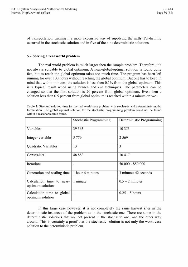
of transportation, making it a more expensive way of supplying the mills. Pre-hauling occurred in the stochastic solution and in five of the nine deterministic solutions. 5.2 Solving a real world problem The real world problem is much larger then the sample problem. Therefore, it’s not always solvable to global optimum. A near-global-optimal solution is found quite fast, but to reach the global optimum takes too much time. The program has been left running for over 100 hours without reaching the global optimum. But one has to keep in mind that within minutes, the solution is less then 0.1% from the global optimum. This is a typical result when using branch and cut techniques. The parameters can be changed so that the first solution is 20 percent from global optimum. Even then a solution less then 0.5 percent from global optimum is reached within a minute or two. Table 3: Size and solution time for the real world case problem with stochastic and deterministic model formulation. The global optimal solution for the stochastic programming problem could not be found within a reasonable time frame.
Stochastic Programming Deterministic Programming
Variables 39 363 10 353
Integer variables 5 779 2 569
Quadratic Variables 13 3
Constraints 48 883 10 417
Iterations - 50 000 - 850 000
Generation and scaling time 1 hour 6 minutes 3 minutes 42 seconds
Calculation time to near-optimum solution
1 minute 0.5 – 2 minutes
Calculation time to global optimum solution
- 0.25 – 5 hours
In this large case however, it is not completely the same harvest sites in the deterministic instances of the problem as in the stochastic one. There are some in the deterministic solutions that are not present in the stochastic one, and the other way around. This is certainly a proof that the stochastic solution is not only the worst-case solution to the deterministic problem.

FSCN/System Analysis and Mathematical Modeling Internet: Http/www.mh.se/fscn
R-03-44 Page 31 (58)
5.3 Value of the uncertainty measures To calculate the values of the uncertainty measures two cases were studied. The difference between the two cases is the cost of storage. In the first, the cost is different for each scenario and approximated to correspond to the drying of the wood in each scenario. This means that in dry weather the storage cost is higher then when it rains a lot. Since the storage costs was a function of time, we had to approximate the differences in cost. Table 4: The value of the different solutions for the real world problem with each scenario having its own storage cost.
Type of solution Value of solution (kkr)
SP 28 024 The deterministic solutions
Scenario 1-1-1 29 197 Scenario 1-1-2 28 130 Scenario 1-1-3 27 380 Scenario 1-2-1 28 653 Scenario 1-2-2 27 480 Scenario 1-2-3 26 791 Scenario 1-3-1 27 991 Scenario 1-3-2 26 696 Scenario 1-3-3 26 858 EEV 27 686 WS 28 230
The value of the stochastic solution (VSS) then becomes (in kkr):
VSS=SP – EEV=28 024 – 27 686= 338 This is approximately 1.2% of the total cost. The expected value of perfect information (EVPI) in kkr: EVPI= WS – SP= 28 230 – 28 024= 206 This is approximately 0.7% of the total cost. In the second case all scenarios had the same storage cost. Off course the cost is still different depending on how long and when it was stored.

FSCN/System Analysis and Mathematical Modeling Internet: Http/www.mh.se/fscn
R-03-44 Page 32 (58)
Table 5: The value of the different solutions for the real world problem where all scenarios had the same storage cost.
Type of solution Value of solution (kkr)
SP 27 847 The deterministic solutions
Scenario 1-1-1 27 149 Scenario 1-1-2 27 242 Scenario 1-1-3 27 620 Scenario 1-2-1 27 351 Scenario 1-2-2 27 480 Scenario 1-2-3 28 126 Scenario 1-3-1 27 377 Scenario 1-3-2 27 493 Scenario 1-3-3 28 146 EEV 27 554 WS 28 019
The value of the stochastic solution (VSS) then becomes (in kkr): VSS=SP – EEV=27 847 – 27 554= 293 This is approximately 1.0% of the total cost. The expected value of perfect information (EVPI) in kkr: EVPI= WS – SP= 28 019 – 27 847= 172 This is approximately 0.6% of the total cost. 6. DISCUSSION AND CONCLUDING REMARKS This model has been represented by two cases, the small sample problem and the large real case problem. The results from the sample problem are not of any great importance, due to the small size of the problem. The meaning with it is just that it should be small enough to be easily presented graphically. This at the same time made it to small to produce any useful results. The large problem does have enough data to produce useful results. It is the results from this problem that really should be evaluated and further discussed. 6.1 The sample problem The difference between the stochastic and deterministic solutions for the sample problem is mainly a question of when to harvest. The areas to harvest in both types of problem are the same, but they are not harvested in the same order. The reason that the

FSCN/System Analysis and Mathematical Modeling Internet: Http/www.mh.se/fscn
R-03-44 Page 33 (58)
same areas are harvested is probably due to the very small problem size and to the fact that a large proportion of the available volume of roundwood is harvested. This limits the number of solutions available. The sites chosen are closest to the mills and usually have good ground and bearing capacity of roads, in other words accessibility. Note, however, that even this restricted problem do not generate the same solution with the deterministic and the stochastic model. 6.2 The real world case problem For the large problem, the stochastic and deterministic models do not always choose the same harvest areas. The solutions are mainly the same, but there are areas in the stochastic solution that are not in the deterministic solution. There are also sites in the deterministic solution that are not present in the stochastic solution. For those that are the same, there are (just as for the sample problem) differences in when they are harvested. The fact that there are harvest sites chosen in the stochastic solution that are not even present in the solutions for the deterministic problem indicates that uncertainty in load-bearing capacity of roads and harvest sites does matter. One must remember that the stochastic programming solution hedges against uncertainty, making the model generate more stable solutions in a real world situation.
One important problem with the stochastic formulation is that it is not possible to solve it to a global optimum, at present, within a reasonable time. What has been called the real case above is only part of the real-world supply chain in that area. It represents one out of five districts supplying a pulp mill in the centre of Sweden. Hence, if we were to use this model to solve the whole supply chain, we would need an alternative approach to making use of a desktop computer. One approach would be to use a cluster of computers to solve smaller parts of the problem. Algorithms are available for this, which solves the stochastic problem by solving many deterministic models in each iteration. This would make it possible to solve larger problems more promptly and with a higher degree of detail in the model. 6.3 Do we need a stochastic model? The value of stochastic solution (VSS) might not be as high as we hoped when we started out working with this model. But, one must remember what this value really means. It is the value for the problems described in this report together with the different costs for every thing such as harvesting, transportation and storage, but only for these exact costs. If one changes these costs the values of VSS and EVPI will also change. Up or down and exactly how much one will never know in advance.
This is one of the aspects of stochastic programming one must not forget. The results are only valid for that instance of the problem. In this report a lot of the costs are approximated, so even if we have worked hard on that these costs should be as realistic as possible, they are probably not correct. They will also vary with the location of the mill, the location of its storage terminal and depend on how exactly the supply chain for that precise mill looks. Whether a stochastic model is needed or not for any given mill can not be decided until one has tested the model for that mill. But, and this is the thing to remember, one can never know if the stochastic model is good or if the deterministic model is sufficient until the stochastic model has been solved. Therefore, to be able to
FSCN/System Analysis and Mathematical Modeling Internet: Http/www.mh.se/fscn
R-03-44 Page 34 (58)
exclude the quality of the solution from the deterministic model, the stochastic model always has to be solved. 6.4 Future extensions There are several aspects of this model that could be improved in the future. Obviously the user would benefit from being able to solve the model faster with more time periods and scenarios. This means that more states of the future could be taken into account. For instance not all bad roads in a district have to be closed when it rains a lot, maybe some will be open longer then others. Hence, more states with different amount of closed roads and harvest sites would be closer to the truth. Technical solutions to bad load-bearing capacity on roads are not incorporated in this model. Techniques as CTI, Central Tire Inflation, is not incorporated due to the problem it leads to from a modelling point of view. The system is being tested with good results, so it should be included in the future. Right now though, it is just not possible to incorporate it without slowing down the computation in a non-acceptable manor. The scheduling of individual harvest teams would be of great interest. It is a very complicated question to solve. The teams’ capacities, abilities and the commuting for the crew have to be taken into consideration. If it could be solved it would lead to a much better utilisation of the harvesting teams. Even if not more time periods or scenarios can be added at this time, there would be benefits with being able to divide the roundwood assortments into more then five categories. From section 2.6 above it is clear that there could be huge profits for the mills if this could be done. Thus, the demand would go from a ‘volume oriented’ view as today to a more ‘fibre oriented’ view in the future. That would mean that the roundwood used for a certain production at the mill would contain fibres that are optimal for that products technical requirement. 7. ACKNOWLEDGEMENTS
We wish to thank the following for financial support, without which this research would not have been possible: FSCN at Mid-Sweden University, the Computer Science Department at Umeå University, the Kempe Foundation, NorFa and the Gunnar Sundblad Research Fund. We also wish to thank and express our gratitude to numerous people at Holmen Skog for answering forestry-related questions, and for providing the dataset. Without the latter, we would not have been able to test our model on a real-world problem. Lastly, we thank Prof. Peter Lohmander at the Swedish University of Agricultural Sciences for many useful discussions, and also advice.

FSCN/System Analysis and Mathematical Modeling Internet: Http/www.mh.se/fscn
R-03-44 Page 35 (58)
APPENDIX A: OPTIMIZATION MODEL A.1 Mathematical formulation To make the reading of the mathematical formulas below easier, there are some pointers as to how the notation should be interpreted.
• p is the probability of some scenario occurring. • All costs are denoted c. To make out what cost is intended one has to look at the
superscript. • Variables and hyper scripts including h have something to do with harvesting
activities. • All variables and hyper scripts including v have something to do with
transportation by truck of the roundwood. • The transportation on rail roads has the notation w. • An activity that has to do with the storage of roundwood uses the notation l. • All letters z and x are decision variables. That means that they are integers (zero
or one).
All the variables and costs will be described in detail in chapter A.2. A.1.1 The objective function min ( ) h
stsh
stsstsTt Sss
hsts
hstssts ttt
t
ttthcphcp ..
1....
..
2..
2.... 111
1
111∑ ∑∈ ∈
+ + (I)
∑∈Tt
ht
fixedht zc , + (II)
∑∑ ∑∈ ∈ ∈Hi Tt
sitscrewh
istsSss
tt
t
hcp ..,
....
11
1
+ (III)
( )∑
∈
+Hi
iitranh zzc 21, + (IV)
∑∑ ∑∈ ∈ ∈Hi Tt
totisits
hlsitssts
Ssshhcp
ttt
t
........
111
1
+ (V)
∑ ∑ ∑ ∑
∈ ∈ ∈ ∈Rji Tt Sss Aaasijts
vsijtssts
t
tttvcp
),( ........
1
111 + (VI)
∑ ∑∈ ∈tt
s tttttttttt
Hi Sss
totissit
phssitsst hhcp
........
1
111 + (VII)
∑∑∑∑ ∑ ∑
∈ ∈ ∈ ∈ ∈ ∈Lj Tk Tu Tt Sss Aaasjkuts
lasjutssts
t
tttlcp
........
1
111 + (VIII)
∑ ∑ ∑ ∑ ∑
∪∈ ∈ ∈ ∈ ∈DLj Rjii Tt Sss Aaasijts
lujsts
t
ttvcp
),(: ......
1
11 + (IX)

FSCN/System Analysis and Mathematical Modeling Internet: Http/www.mh.se/fscn
R-03-44 Page 36 (58)
∑ ∑ ∑ ∑ ∑
∈ ∈ ∈ ∈ ∈Lj Rjii Tt Sss Aaasjits
lljsts
t
ttvcp
),(: ......
1
11 + (X)
∑
∈Lj
lj
fixedlj zc , + (XI)
∑∑ ∑ ∑∈ ∈ ∈ ∈Dj Tt Sss Aa
dasjts
edasjtssts
t
tttecp
........
1
111 + (XII)
∑∑ ∑ ∑∈ ∈ ∈ ∈Dj Tt Sss Aa
dasjts
fixededasjtssts
t
tttecp
....
,....
1
111 + (XIII)
∑∑ ∑ ∑∈ ∈ ∈ ∈Dj Tt Sss Aa
iasjts
eiasjtssts
t
tttecp
........
1
111 + (XIV)
∑ ∑∈ ∈
−sDj Aa
sja
yj yc )1( + (XV)
∑
∈ RRji
wij
fixedwij zc
),(
, + (XVI)
∑ ∑ ∑ ∑∈ ∈ ∈ ∈R
t
t
Rji Tt Sss Aacij
asijtswij w
wc
),( ..
..
1
1 + (XVII)
( )∑ ∑ ∑
∈ ∈ ∈Ft
ttRji Tt Sss
fsijts
fijsts vcp
, ......
1
11 (XVIII)
A.1.2 The constraints
tt sitssits yh .... 11≤ SsTtHHi tt
s ∈∈−∈∀ ,, (1a)
t
ttt
tasissits yy
111 ..... −≤ tt
ts tttSsHi t ,1;, −=∈∈∀ (1b)
1..1
≤∑∈Tt
sits th SsHi ∈∈∀ , (2)
1
.. 21 i
Ttsits zy
t≤∑
∈
SsHHi tts ∈−∈∀ , (3a)
1
....... 21111 i
Tvsivs
tasis
Tusius zyyy
t
t
ttt≤++ ∑∑
∈∈−
SsHi tts ∈∈∀ , (3b)
)1(..)1(.. 1
111 ++ +≤++ titsstisits zyy
tt n
ts ttSsTtHHi t <∈∈−∈∀ ;,, (4a)

FSCN/System Analysis and Mathematical Modeling Internet: Http/www.mh.se/fscn
R-03-44 Page 37 (58)
)1(..)1(.. 1
111 ++ +≤++ titsstisits zyy
tt 2;,, −<∈∈∈∀ t
ts ttSsTtHi t (4b)
( ) ( )( )12.....2 1
111 −−− +≤+− tt
t
tttt ttit
asisssti zyy SsTtHi tts ∈∈∈∀ ,, (4c)
)1(..)1(.. 1
11 ++ +≤+ titsstisits zyytt
ntts tttSsTtHi t <<∈∈∈∀ ;,, (4d)
1max...
)1(1 +≤∑
∈+
t
t
t
hsts
Hitit h
hz nttSsTt <∈∈∀ ;, (5)
2
.... 111 isiussits zyy
ut+≤+ 1;,,, +>∈∈∈−∈∀ tuSsTuTtHHi tt
s (6a)
2.... 1
11 isiussits zyyut
+≤+
ttts ttuttuSsTuTtHi t ,1,;1;,,, −≠+>∈∈∈∈∀ (6b)
2
..... 1111 isius
tasis zyy
u
t
tt+≤+
−
2;;,,, −<>∈∈∈∈∀ ttts tutuSsTuTtHi t (6c)
h
stsHi
sitsf
Hic
sits
totisits
tt
t
t hyth
hh....
..
..11
1
1 =+ ∑∑∈∈
tt tttSsTt ,1;, −≠∈∈∀ (7a)
( )
( )( ) ( )
hsst
Hic
ssit
totissit
Hissti
f
Hic
ssti
totissti
ttttt
s ttt
ttt
ttt
ttt
ttt hh
hhyt
h
hh11
1
1
11
11
11
..1..
....1
..1
..1
−−
−
−
−∈∈
−∈ −
−=++ ∑∑∑ Ss ∈∀ (7b)
h
stsHi
sitsf
HHic
ssit
totissit
tttttt
s ttt
ttt hyth
hh....
..
..
11
1
1 =+ ∑∑∈−∈
Ss ∈∀ (7c)
ht
hct
hsts
hct zh
tmaxmin ..1
≤≤ SsTt ∈∈∀ , (8)
( ) ( )
toti
partiasits
Rijasjits
Rjiasijts hhhvv
ttt ..,
..,
.. 111=− ∑∑
∈∈
AaSsTtHi ∈∈∈∈∀ ,,, (9)
( ) ( )0
,..
,.. 11
=− ∑∑∈∈ Rji
asijtsRij
asjits ttvv AaSsTtCi ∈∈∈∈∀ ,,, (10)
tot
sijtsAa
asijts ttrv .... 11
≤∑∈
( ) SsTtRji ∈∈∈∀ ,,, (11)

FSCN/System Analysis and Mathematical Modeling Internet: Http/www.mh.se/fscn
R-03-44 Page 38 (58)
( )
vct
Rji Aa
tsijtsc
sijts
asijts
Lj Aa
llasjits
DLj Aa
luasijts
Hi Aa
hlasijts
vct t
t
t
tttt
vv
tvtvtv maxmin,
....
........ 1
1
1
111≤+++≤ ∑ ∑∑∑∑ ∑∑∑
∈ ∈∈ ∈∪∈ ∈∈ ∈
SsTt ∈∈∀ , (12)
( ) ( )0..112
,1
,1 1
=−−+ ∑∑∈∈
assjRji
ajiRji
aijinitja u
lvvl AaSsLj ∈∈∈∀ ,, (13)
( )( ) ( )
( ) 0212121211
1
11 ..1,
..,
......1 =−−+ ∑∑∑∑ ∑∈
+∈∈∈ ∈
−Tk
asstjktRij
asjitasRji
asijtsa
aasjktsTk Aa
aststjk uttuulvvxl
tkAaSsTtLj <∈∈∈∈∀ ;,,, 2 (14)
( )( ) ( )
0..,
..,
......1 122121211
1
11=−−+ ∑∑∑ ∑
∈∈∈ ∈−
finalssja
Rijassjit
Rjiassijt
aaassjkt
Tk Aaassttjk ntntnntnununn
lvvxl
ntkAaSsLj <∈∈∈∀ ;,, 2 (15)
( )∑∑∈ ∈
+ ≤Aa Tk
ljjtasstjkt zll
u
max..1 1
tkSsTtLj ≤∈∈∈∀ ;,, (16a)
( ) ( ) asstjktaststjk uu
ll ..1..1 11 +− ≥ tkAaSsTtTkLj ≤∈∈∈∈∈∀ ;,,,, (16b)
( ) 0..1 1
=+ asstjkt ul
tkAaSsTtTkLj >∈∈∈∈∈∀ ;,,,, (16c)
∑∑∈ ∈
≤Tv Tu
asjvusjta ull ..
min1
tutvAaSsTtLj >≤∈∈∈∈∀ ,;,,, (17a)
final
asjsajt ntnll ..
min1
≤ AaSsLj ∈∈∈∀ ,, (17b)
max,min, okta
okta
okta ddd ≤≤ AaTtOk ∈∈∈∀ ,, (18)
( )2
1
211212121 ....,
.. jtaOk Aa
sakja
okta
iasjts
dasjts
Rjiasijts dxdeev
ttt=+++ ∑ ∑∑
∈ ∈∈
AaSsTtDj ∈∈∈∈∀ 2,,, (19)
totjt
Aajtajta dd =∑
∈
α TtDj ∈∈∀ , (20)
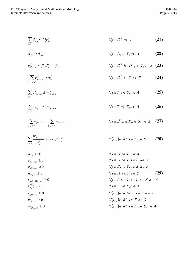
FSCN/System Analysis and Mathematical Modeling Internet: Http/www.mh.se/fscn
R-03-44 Page 39 (58)
sja
Ttjta Myd ≤∑
∈
AaDj S ∈∈∀ , (21)
ljtajta dd ≥ AaTtDj ∈∈∈∀ ,, (22)
jt
totjtj
fsjits fdv
t+≤ β..1
SsTtDiDj PS ∈∈∈∈∀ ,,, (23)
( )
fjt
Rji
fsijts dv
ft
≥∑∈,
..1 SsTtDj P ∈∈∈∀ ,, (24)
d
astsDj
dasjts tt
me .... 11≤∑
∈
AaSsTt ∈∈∈∀ ,, (25)
i
astsDj
iasjts tt
me .... 11≤∑
∈
AaSsTt ∈∈∈∀ ,, (26)
( ) ( )∑∑
∈∈
=R
ttRij
asjitsRji
asijts wv,
..,
.. 11 AaSsTtLj W ∈∈∈∈∀ ,,, (27)
wij
wct
Aacij
asijts zw
wt max..1 ≤∑
∈
( ) SsTtRji R ∈∈∈∀ ,,, (28)
0≥jtad AaTtDj ∈∈∈∀ ,,
0..1≥d
asjts te AaSsTtDj ∈∈∈∈∀ ,,,
0..1≥i
asjts te AaSsTtDj ∈∈∈∈∀ ,,,
0..1≥
tsitsh SsTtHi ∈∈∈∀ ,, (29)
( ) 0..1 1≥+ asstjkt t
l AaSsTtTkLj ∈∈∈∈∈∀ ,,,, 0..1
≥finalasjs nt
l AaSsLj ∈∈∈∀ ,, 0..1
≥asijts tv ( ) AaSsTtRji ∈∈∈∈∀ ,,,,
0..1≥f
sijts tv ( ) SsTtRji F ∈∈∈∀ ,,,
0..1≥asijts t
w ( ) AaSsTtRji R ∈∈∈∈∀ ,,,,

FSCN/System Analysis and Mathematical Modeling Internet: Http/www.mh.se/fscn
R-03-44 Page 40 (58)
{ }1,0..1∈
tsitsy SsTtHi ∈∈∈∀ ,, { }1,0∈s
jay AaDj S ∈∈∀ , { }1,0
11... ∈−
t
tt
tasisy AaSsDi S ∈∈∈∀ ,,
{ }1,0)1( ∈+titz nttTtHi <∈∈∀ ;,
{ }1,01 ∈iz Hi ∈∀ (30) { }1,02 ∈iz Hi ∈∀ { }1,0∈l
jz Lj ∈∀
{ }1,0∈htz Tt ∈∀
{ }1,0∈wijz ( ) RRji ∈∀ ,
A.2 Definitions In the mathematical model several sets, parameters and variables are used. They are here presented in groups and explained. A.2.1 Sets A = Assortments C = Cross roads D = Mills
SD = Saw mills, a subset of D. PD = Pulp and Paper mills, a subset of D.
H =Harvest sites tt
sH = Harvest sites that can’t be harvested during period tt , scenario s, due to thawing, a subset of H. L = Terminals
WL = Train terminals O = Mills own by other companies. R = Roads
FR = Roads for transporting wood chips RR = Rail roads
S = Scenarios T = Time periods A.2.2 Parameters
jtaα = A parameter that describes how much useful fibre there are in assortment a in time period t at mill j.
jβ = The relative part of the demand at a saw mill j that will be turned into wood chips.
ljtγ = Calculated part of the volume bought from the domestic market where the buyer
FSCN/System Analysis and Mathematical Modeling Internet: Http/www.mh.se/fscn
R-03-44 Page 41 (58)
have to pay the transport. fjtd = Minimum demand of wood chips at pulp/paper mill j for period t. ljtad = Minimum demand of assortment a at mill j for period t.
max,oktad = Maximum volume, of assortment a, that can be delivered to mill k for period t.
min,oktad = Minimum volume, of assortment a, that has to be delivered to mill k for
period t. totjtd = Total minimum demand of all assortments at mill j for period t.
jtf = The volume of wood chips produced from wood delivered by other contractors to mill j for period t.
csits t
h ..1= Capacity at location i for scenario (s1,s2,…,st) during period t. Must be greater
than zero. maxth = The maximum number of harvesting hours a team can work in time period t. part
iah = The proportion of the total volume at site i that consist of assortment a. totih = The total volume at site i that can be harvested. initjal = The initial stored volume of roundwood of assortment a at terminal j. maxjtl = The maximal volume terminal j can hold at any given time period t. minjtal = The minimal volume of assortment a that terminal j must hold at any given time
during period t. M = A large number used to set some binary variables (for instance 100 000).
dasts t
m ..1= Total volume of assortment a that can be bought on the domestic market for scenario (s1,s2,…,st) during period t due to logistic constraints.
iasts t
m ..1= Total volume of assortment a that can be bought on the international market for scenario (s1,s2,…,st) during period t.
hct
hct max,min = Minimum and maximum harvesting capacity, in hours, during period t.
vct
vct max,min = Minimum and maximum transportation capacity, in hours, during
period t. wctmax = Maximum number of railway wagons available for period t.
tstsp ..1= Probability of scenario (s1,s2,…,st) in period t.
totsijts t
r ..1= Maximum volume that can be transported on road (i,j) for scenario (s1,s2,…,st)
during period t. nt = The last time period.
tt = The time period that contains the thawing period. ft = Average transportation time between harvesting sites. hlt = Loading time at harvest site, in average, per volume transported by truck. llt = Loading time at storage terminals, in average, per volume transported by truck. lut = Unloading time and time it takes to measure the delivered volume at a terminal or
mill for roundwood delivered by truck.

FSCN/System Analysis and Mathematical Modeling Internet: Http/www.mh.se/fscn
R-03-44 Page 42 (58)
tsijts t
t ..1 = Travel time for road (i,j) for scenario (s1,s2,…,st) during period t.
csijts t
v ..1= Loading capacity for trucks on road (i,j) for scenario (s1,s2,…,st) during period
t. Must be greater than zero. cijw = Loading capacity for railway wagons on railroad (i,j). Must be greater then zero. a
aasiuts tx
211.. = A parameter that tells if roundwood stored from time period u to period t will change assortment from a1 to a2 in scenario (s1,s2,…,st). Can also represent a part of the volume.
sakjtax
21= A parameter that tells if roundwood of assortment a1 delivered to mill k
will be transferred as assortment a2 to mill j. Can also represent a part of the total volume. A.2.3 Costs Some of the costs included in this model are not dependent on a certain volume of roundwood. Either the cost takes place or not. These costs are considered as fixed costs. One should note that most fixed costs still are optional, i.e. they don’t have to occur. However, most costs are connected to the volume of roundwood transported, harvested and so on. The two different types of costs are divided into different groups to make it easier to identify them. A.2.3.1 Fixed costs
fixededasjts t
c ,..1
= The cost of transporting assortment a, bought on the domestic market, to mill j for scenario (s1,s2,…,st) during period t.
crewhic , = A fixed cost for transportation of the crew to and from the harvest area.
fixedhtc , = The fixed cost for harvesting during period t.
tranhc , = The cost of transportation of internal equipment between harvesting sites. fixedl
jc , = The cost of operating terminal j. fixedw
ijc , = The fixed cost per train set on railroad from i to j. yjc = The cost of having an extra assortment a at saw mill j.
A.2.3.2 Volume dependent costs
edasjts t
c ..1= The cost of buying assortment a on the domestic market for mill j in scenario (s1,s2,…,st) during period t.
eiasjts t
c ..1= The cost of buying assortment a on the international market for mill j for
scenario (s1,s2,…,st) during period t. f
ijc = The cost of transporting wood chips from saw mill i to pulp/paper mill j. 1..1
hsts t
c = The linear cost for harvesting scenario (s1,s2,…,st) during period t. 2..1
hsts t
c = The quadratic cost for harvesting scenario (s1,s2,…,st) during period t.

FSCN/System Analysis and Mathematical Modeling Internet: Http/www.mh.se/fscn
R-03-44 Page 43 (58)
hlsits t
c ..1= The cost of loading the harvested roundwood at harvest site i for scenario
(s1,s2,…,st) during period t. l
asjuts tc ..1
= The cost of storing at terminal j from time period u to time period t with scenario (s1,s2,…,st) for assortment a without watering.
lljc = The cost of loading at terminal j. lujc = The cost of unloading at terminal or mill j. ph
sits tc ..1
= The cost of pre-hauling the harvested roundwood to an accessible road for areas that can’t be accessed during the thawing period in the spring.
vsijts t
c ..1= The cost for transport on road (i,j) for scenario (s1,s2,…,st) during period t.
wijc = The cost of transportation on railroad form i to j, dependent on volume transported.
A.2.4 Variables There are two different types of variables in this model. The most common one is the continuous variables. They are used when volume is flowing in the network or to denote how much of a harvest site that is harvested. The other type is binary variables. These are decision variables. That is they represent whether a decision is taken or not. This could be if a harvest site is harvested or not. A.2.4.1 Continuous variables
jtad = Volume of assortment a used at mill j for period t. oktad = Volume of assortment a transported to mill k, owned by another company, for
time period t. d
asjts te ..1
= Volume of assortment a bought on the domestic market at mill j for scenario (s1,s2,…,st) during period t.
iasjts t
e ..1 = Volume of assortment a bought on the international market at mill j for
scenario (s1,s2,…,st) during period t.
tsitsh ..1 = Part of area i harvested in scenario (s1,s2,…,st) during time period t.
hsts t
h ..1= Number of hours used for harvesting in scenario (s1,s2,…,st) during period t.
asjkuts tl ..1
= Volume of assortment a stored at j for scenario (s1,s2,…,st) from period u to t that initially was stored during period k.
finalasjs nt
l ..1= The volume of assortment a that is in store at the end of time period tn with
scenario (s1,s2,…,stn). asijts t
v ..1 = Volume of assortment a transported on road (i,j) for scenario (s1,s2,…,st)
during period t.
fsijts t
v ..1 = Volume of wood chip transported from saw mill i to pulp/paper mill j in
scenario (s1,s2,…,st) during period t. asijts t
w ..1= Volume of assortment a transported on railroad (i,j) for scenario (s1,s2,…,st)

FSCN/System Analysis and Mathematical Modeling Internet: Http/www.mh.se/fscn
R-03-44 Page 44 (58)
during period t. A.2.4.2 Binary variables
tsitsy ..1= Is 1 if the area is harvested during time period t with scenario (s1,s2,…,st)
otherwise 0. sjay = Is 1 if the assortment is in use at the saw mill otherwise 0. t
tt
tasisy
11... −= I 1 if either ( ) 11..1 −− ttt sstiy or
ttt ssity ..1 is 1 otherwise 0.
)1( +titz = Is 1 if tsitsy ..1 or any of
11..)1( ++ tsstiy is 1 otherwise 0. 1iz = Is 1 if any of )1( +titz is 1 otherwise 0. 2iz = Is 1 if
tsitsy ..1 and
usiusy ..1 is 1 and u>t+1 otherwise 0.
htz = Is 1 if anything is harvested during period t otherwise 0. ljz = Is 1 if anything is stored at storage j during any time period and scenario,
otherwise 0. wijz = Is 1 if anything is transported on railroad from i to j.

FSCN/System Analysis and Mathematical Modeling Internet: Http/www.mh.se/fscn
R-03-44 Page 45 (58)
APPENDIX B: ESTIMATION OF COSTS B1: HARVEST COSTS FROM THE OWN FOREST The cost for a machine group, that is one harvester and one forwarder working together in a team, consists of three parts.
1. Initial or fixed cost for having and operating a machine group. These are typically the cost for buying the machines, insurance and so on.
2. Hour costs for operating the machine group. In this category one finds cost for crew, maintenance, operations and so on.
3. The last is the cost of travel costs for the crew. Every crew member gets paid to travel to where the actually harvesting takes place from his or hers home-base. In the future when we talk about harvesting cost, we will only talk about the
costs in points one and two. The cost in point three will be handled separately in the model. A restriction to the model is that we assume that we use a machine group as much as possible before employing another team. By this we mean that the existing team will work overtime before we contract any new team. Since overtime comes with a higher cost, this gives the cost function an ugly appearance.
Figure B.1.1: The harvesting cost. The dotted line is the approximation of the real cost for harvesting using several machine groups. The real cost is depicted with the thick line.

FSCN/System Analysis and Mathematical Modeling Internet: Http/www.mh.se/fscn
R-03-44 Page 46 (58)
It might not be that easy to see, but the cost is here approximated with a quadratic function. To see this better, the cost is approximated for only two working machine groups instead for ten as in figure A.1.1.
Figure B.1.2: The harvesting cost for only two machine groups. The dotted line is the approximation of the cost. It is more easily to see that this is a quadratic function.
This cost function is no longer linear. However, the function can be
approximated with a second degree equation and then becomes convex and quadratic. Hence, it will not add any major difficulties for the solver.
Figure B.1.1 is, of course, a very simplified picture of the harvesting activities. There are many aspects not considered. For one, it is probably not the best decision, all though it is completely feasible, to have several machine groups working overtime when there are other machine groups available. In the long run it would maybe be better to hire another machine group, both economically and for the workers. The total number of over time hours a worker is allowed to work per year is limited in Sweden. Therefore one should be careful to use overtime since it might limit future actions.
Which one that is the best decision, overtime or another machine group, is dependent on the situation. Harvest at the present sites, as well as the demand at mills has to be considered. Are there possibilities for opening another harvest site of any kind? Is there a site where a second harvesting team can work?
In many ways is Figure B.1.1 simplified. Nevertheless, to really determine the actual cost we have to involve simulations of the possible scenarios to determine a really good cost function.

FSCN/System Analysis and Mathematical Modeling Internet: Http/www.mh.se/fscn
R-03-44 Page 47 (58)
B2: TRANSPORTATION COSTS The transportation cost for the roundwood will differ depending on in which scenario and time period it takes place, and transport is also uncertain. Since roads may be closed during some scenarios. In table B.2.1, based on Lohmander & Olsson (2003), it is shown when roads of different classifications are open or closed. Table B.2.1: Times when the roads of different classes are open or closed.
Road class
Winter Spring LOW
Spring MED
Spring HIGH
Summer LOW
Summer MED
Summer HIGH
A Open Open Open Open Open Open Open B Open Open Open Closed Open Open Open C Open Open Closed Closed Open Open Closed D Open Closed Closed Closed Open Closed Closed The cost of transportation may not be the same during all the scenarios when the roads are open for transport. The reason is that more maintenance is needed or that the trucks can’t drive with a full load due to load-bearing restrictions. The costs are based on Lohmander & Olsson 2003. Table B.2.2: The cost for transportation on different types of roads in different scenarios and time periods. The cost is divided into one fixed and one variable part where L is the length of the road. Based on the cost estimations in Lohmander & Olsson 2003.
Road class
Winter Spring LOW
Spring MED
Spring HIGH
Summer LOW
Summer MED
Summer HIGH
A 12+0.4L 12+0.4L 14+.45L 15+0.55L 12+0.4L 12+0.4L 14+0.45LB 12+0.4L 12+0.4L 14+.45L Closed 12+0.4L 12+0.4L 14+0.45LC 14+0.45L 15+0.55L Closed Closed 14+0.45L 15+0.55L Closed D 15+.55L Closed Closed Closed 17+0.65L Closed Closed B3: ROUNDWOOD STORAGE COSTS The cost of storage plays an important roll in the procurement of pulp mills. If it is low, the storages can be larger, and if it is high they must be smaller. The exact cost will depend on the location of the storage itself, when the roundwood first was put into the storage, when it is removed from the storage, in what weather conditions it is stored but also what time of the year it is. As a base for the storage costs, we have used figures specified for timber, hardwood pulp and softwood pulp estimations by the forest research institute of Sweden (Arvidsson & Holmgren 1999). They are depicted in Figures B.3.1 thru B.3.3

FSCN/System Analysis and Mathematical Modeling Internet: Http/www.mh.se/fscn
R-03-44 Page 48 (58)
Figure B.3.1: The storage cost for timber. The stars mark the predicted cost by the forest research institute of Sweden. The line is a least square approximation of these estimates.

FSCN/System Analysis and Mathematical Modeling Internet: Http/www.mh.se/fscn
R-03-44 Page 49 (58)
Figure B.3.2: The storage cost for Hardwood. The stars mark the predicted cost by the forest research institute of Sweden. The line is a least square approximation of these estimates.

FSCN/System Analysis and Mathematical Modeling Internet: Http/www.mh.se/fscn
R-03-44 Page 50 (58)
Figure B.3.3: The storage cost for softwood. The stars mark the predicted cost by the forest research institute of Sweden. The line is a least square approximation of these estimates.
The basic idea is that the cost is closely related to the degree of dehydration in the roundwood. Based on these costs and rough estimates of how the dehydration will differ in the scenarios, new costs for the storage were calculated. The dehydration was based on figures presented in Forsberg (2000). Table B.3.1: The relative dehydration in percent. The figures are based on the local conditions in Piteå, but since they are located in a similar environment (SUAS) as the mill used in the real world case in this report, it should be a good approximation.
Month May June July August September Dehydration 14% 18% 25% 18% 4%
In the tables below the first column to the left indicates which time period the roundwood was put into storage. The top row shows the time period1 and scenario2 of when the roundwood is taken out of storage. Knowing these two parameters gives us the history of the roundwood. The scenarios are denoted with the following numbers: 1 The time period is indicated as the first number. 2 The scenarios are indicated by the figures that follows the time period. For the roundwood that is taken out of storage in time period two, only one scenario is needed, i.e. the scenario in time period two. If the roundwood is stored until the third time period, the scenario in the second period is indicated by the figure in the middle and the scenario in the third time period by the last figure.

FSCN/System Analysis and Mathematical Modeling Internet: Http/www.mh.se/fscn
R-03-44 Page 51 (58)
1: Dry scenario 2: Normal scenario 3: Wet scenario Table B.3.2: The storage cost for softwood. Since everything is frozen in the winter and frozen roundwood stay frozen even as it gets warmer in the spring, there is not any difference in storage cost between the scenarios in time period 2.
2,1 2,2 2,3 3,1,1 3,1,2 3,1,3 3,2,1 3,2,2 3,2,3 3,3,1 3,3,2 3,3,31 18 18 18 130 97 66 108 72 37 89 49 40 2 - - - 110 77 46 88 52 17 69 29 18
Table B.3.3: The storage cost for hardwood. Since everything is frozen in the winter and frozen roundwood stay frozen even as it gets warmer in the spring, there is not any difference in storage cost between the scenarios in time period 2.
2,1 2,2 2,3 3,1,1 3,1,2 3,1,3 3,2,1 3,2,2 3,2,3 3,3,1 3,3,2 3,3,31 18 18 18 114 86 59 96 64 35 79 46 41 2 - - - 94 66 39 76 44 15 59 25 19
Table B.3.4: The storage cost for timber. Since everything is frozen in the winter and frozen roundwood stay frozen even as it gets warmer in the spring, there is not any difference in storage cost between the scenarios in time period 2.
2,1 2,2 2,3 3,1,1 3,1,2 3,1,3 3,2,1 3,2,2 3,2,3 3,3,1 3,3,2 3,3,31 57 57 57 103 99 94 100 96 92 98 93 98 2 - - - 43 39 34 40 36 32 38 33 38
B4: TOTAL COST FOR IMPORT AND DOMESTIC ROUNDWOOD
Table I and II below summarize the cost of roundwood at the domestic and the import market. However, an additional cost for quality losses is also added, as described in Appendix B.3.
Table B.1: Import prices on international market 2001 (SVO).
TT2001ie GT2001ie BM2001ie GM2001ie LM2001ie 1:a kv. 455 425 358 335 345 2:a kv 450 421 354 331 350 3:e kv 422 394 332 310 325 4:e kv. 455 425 358 335 334
Table B.2: Prices on the domestic roundwood market 2001 (SVO).
TT2001m GT2001m BM2001m GM2001m LM2001m 1:a kv. 399 376 249 235 229 2:a kv 387 361 250 235 229 3:e kv 393 365 244 228 222 4:e kv. 409 378 231 227 218

FSCN/System Analysis and Mathematical Modeling Internet: Http/www.mh.se/fscn
R-03-44 Page 52 (58)
APPENDIX C: OPTIMAL ROTATION TIME FOR SAFETY STOCK There are several reasons to store roundwood. In Hägg (1991) the stored volume are divided into the following groups:
1. Process inventory 2. Business inventory 3. Productivity inventory 4. Safety inventory
The first kind of inventory is needed to run the process at the mill. The business
inventory is there to give a lower cost for external purchases. Productivity inventory are there to give a lower total production cost for the forest operations. Finally the safety inventory is there to make sure that the mill never run out of roundwood supplies.
In this section, only the safety inventory will be considered. There are some, for instance Koskinen (2000), arguing that the safety stock should be minimized. In Persson (2001) it is suggested that the safety stock should not be minimized but optimized. In the model presented in this report the three first inventory types are considered as one, in order to optimize them. There are two ways of treating the safety stock in the model
1. Include it together with the rest of the storage. To ensure that to model always
will keep enough of each assortment in store, minimum levels can be set. 2. It can be considered as a completely separately storage and not included in the
model at all. The minimum levels for different assortment and time periods may still be set.
It is put forward by Persson (2001) that this volume of roundwood should
probably be replaced from time to time. If the first approach to the safety inventory is chosen the replacement of the stock will be handled by the model. The solution will tell us in which time periods to exchange the stored volume. The second approach leaves the model without control over the safety stock, making it impossible to decide time of replacement. In this appendix it will be shown, using existing costs, how often the safety stock, in the second approach, should be replaced during the year.
Since the cost of storing is dependent on how quickly the roundwood dries out, the cost will vary during the year. Hence the economically optimal time interval to replace the safety inventory will also vary during the year. The dehydration of the roundwood varies not only with the time of year, but also with geographical location and local conditions at the storage facility.
The purpose of this appendix is to show how to calculate the optimal replacement time. We will use existing figures for the cost of storing roundwood given by Arvidsson & Holmgren (1999) for softwood (Figure A3.3) used in the making of pulp or paper.
Besides the cost for storage of the roundwood there are several other costs and data needed for this optimization, they are taken from Forsberg (2000). The costs are all in SEK and the volume is measured as the volume of sold under bark, shorten as s.u.b. below.
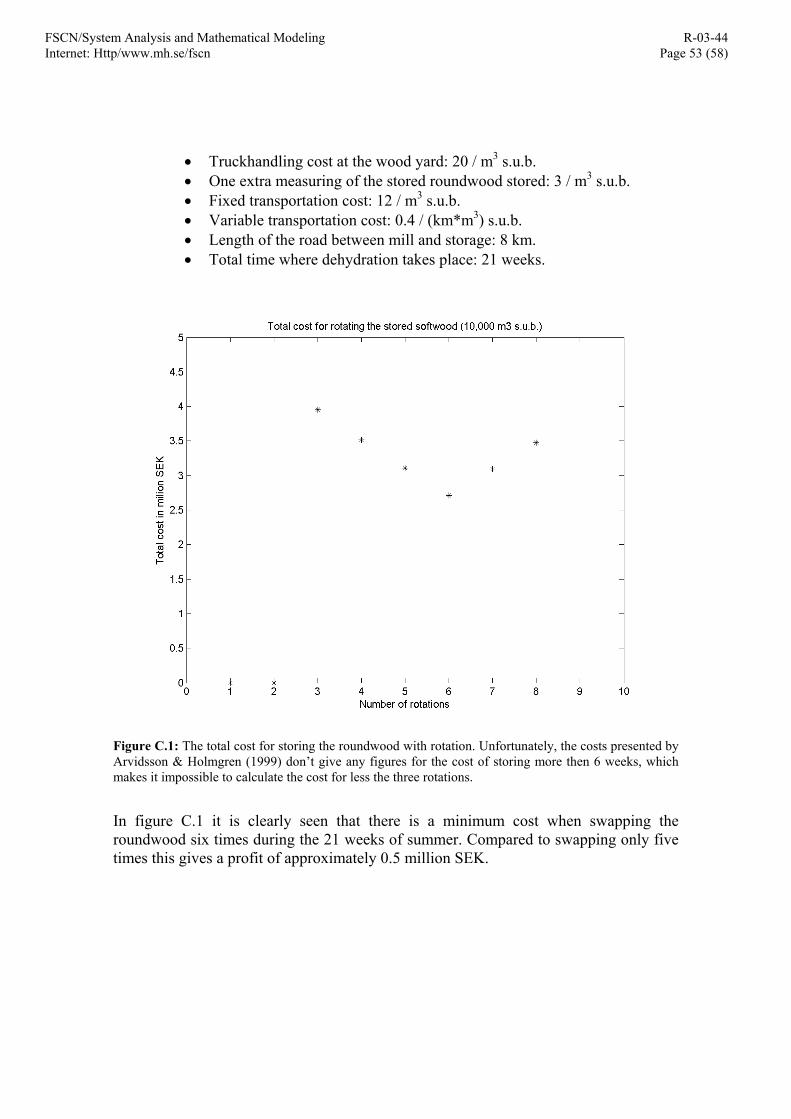
FSCN/System Analysis and Mathematical Modeling Internet: Http/www.mh.se/fscn
R-03-44 Page 53 (58)
• Truckhandling cost at the wood yard: 20 / m3 s.u.b. • One extra measuring of the stored roundwood stored: 3 / m3 s.u.b. • Fixed transportation cost: 12 / m3 s.u.b. • Variable transportation cost: 0.4 / (km*m3) s.u.b. • Length of the road between mill and storage: 8 km. • Total time where dehydration takes place: 21 weeks.
Figure C.1: The total cost for storing the roundwood with rotation. Unfortunately, the costs presented by Arvidsson & Holmgren (1999) don’t give any figures for the cost of storing more then 6 weeks, which makes it impossible to calculate the cost for less the three rotations.
In figure C.1 it is clearly seen that there is a minimum cost when swapping the roundwood six times during the 21 weeks of summer. Compared to swapping only five times this gives a profit of approximately 0.5 million SEK.

FSCN/System Analysis and Mathematical Modeling Internet: Http/www.mh.se/fscn
R-03-44 Page 54 (58)
REFERENCES 1. Aarts, E., Lenstra, J. K. 1998. Local search in combinatorial optimization, John
Wiley & Sons Ltd, Chichester, England.
2. Amram, M., Kulatilaka, N. 1999. Real options: Managing strategic investment in an uncertain world. Harvard business school press, Boston, USA.
3. Andersson, K. 2001. Sulfatmassatillverkningens ekonomi, del 1. Skogsindustrins Utbildning i Markaryd AB, X-720.
4. Anon. 1999a. Sambandet är entydigt: Färskt, friskt virke = ljust, fint papper. Aktivt skogsbruk, 1999:1
5. Anon. 1999b. Från stort virkeslager till precis-i-tid Aktivt skogsbruk, 1999:5
6. Anon. 2002. Lingo - The modelling language and optimizer. Lindo Systems Inc, Chicago, Illinois, USA.
7. Arlinger, J., Spånberg, K., Wilhelmsson, L., Lundqvist, S.0., Hedenberg, Ö., Jonasson, J., Jansson, U. 2000. Vedegenskaper för massaindustrins behov. Redogörelse 2, The Forestry Research Institute of Sweden.
8. Arlinger, J., Wilhelmsson, L. 1998. Fiberkunskap för ökad lönsamhet. Redogörelse 1998:5, The Forestry Research Institute of Sweden.
9. Arvidsson, P-Å, Eriksson, I., Eriksson, P., Rönnqvist, A., Westerlund, A., Igeklint, P. 1999. Smartare vägval i skotningen - bra för både ekonomi och miljö, Resultat Nr. 22, SkogForsk, Uppsala, Sweden.
10. Arvidsson, P-Å., Forsberg, M., Jönsson, A., Flisberg, P., Rönnqvist, M. 2000. Beslutsstöd för investeringar i bärighetshöjande åtgärder (BIT), The Forestry Research Institute of Sweden, Report Nr 470.
11. Arvidsson, P-Å., Holmgren, M. 1999. Vägstandardens inverkan på skogsnäringens transportarbete och försörjning av högkvalitativa råvaror. Arbetsrapport 433, The Forestry Research Institute of Sweden.
12. Barros, O., Weintraub, A. 1982. Planning for vertically integrated forest industries. Operations Research 30(5) 1168-1182.
13. Berg, M., Bjurulf, A., Duchesne, I., Hedenberg, Ö., Löfgren, M. 1995a. Vad är färskhet? The Forestry Research Institute of Sweden, Result No 5, 1995.
14. Berg, M., Bjurulf, A., Löfgren, M. 1995b. Uppdelning av granmassaved efter egenskaper. The Forestry Research Institute of Sweden, Result No 6, 1995.
15. Berg, M., Larsson, L. 1994. A planning system for timber transport optimisation at Södra. Arbetsrapport 190, Inst. f. Skogsekonomi, SUAS.
16. Bergdahl, A. 2002. Optimal destination of saw timber in northern Sweden : important factors for potential. Working report No 53??, Skogsteknologi??, SUAS, Sweden.

FSCN/System Analysis and Mathematical Modeling Internet: Http/www.mh.se/fscn
R-03-44 Page 55 (58)
17. Bergman, M. 1998. Virkespriser och svensk virkesmarknad. Working report No 80 SUAS, Sweden.
18. Bergström, J. 2001. Manual - SkogForsk Vägbåtnad 2.0, ver 1.1. Manual, The Forestry Research Institute of Sweden.
19. Bergström, J., Brunberg, B. 2000. Gasa och bromsa i turordningsplaneringen! Redogörelse 2000:2, Forestry Research Institute of Sweden.
20. Birge, J. R., Louveaux, F. 1997. Introduction to stochastic programming. Springer-Verlag Telos.
21. Blom, G. 1984. Sannolikhetsteori med tillämpningar. Studentlitteratur, Lund, Sweden.
22. Bredström, D., Lundgren, J. T., Rönnqvist, M., Carlsson, D., Mason, A. 2001. Supply chain optimization in the pulp mill industry. LiTH-MAT-R-2001-12, Linköping University, Sweden.
23. Brunberg, T., Arlinger, J. 2001. Vad kostar det att sortera virket i skogen? Resultat nr 3 SkogForsk, Uppsala, Sweden.
24. Carlgren, C-G., Carlsson, D., Rönnqvist, M. 2000. Selection of sorting strategies in harvesting integrated with backhauling, LiTH-MAT-R-2000-18, Linköping University, Sweden.
25. Carlsson, D., Rönnqvist, M. 2001. Tactical planning of forestry transportation with respect to backhauling, LiTH-MAT-R-1998-13, Linköping University, Sweden.
26. Carlsson, D., Rönnqvist, M., Westerlund, A. 1998. Extraction of logs in forestry using operations research techniques, LiTH-MAT-R-1998-17, Linköping University, Sweden.
27. Courdeau, S.F., Pasin, F., Soloman, M.M. 2003. An integrated model for logistics network design, Collection of articles: NorFA research seminar course in multi-model transportation in quantitative logistics, Håholmen by Molde, April 23-May 2, 2003.
28. Cranic, T.G. 1998. A survey of optimization models for long haul freight transportation, publ CRT-98-67, Centre de recherché su les transports, Univerite´ de Montréal
29. Forsberg, M. 2000. Optimalt virkeslager, Working report No 291. Dept. Of Forest Economics, SUAS, Sweden.
30. Forsgren, Å. 1993. Returtransport av rundvirke. SUAS, Sweden.
31. Gong, P. 1998. Optimal harvest policy with first-order autoregressive price process, Working report No 257. Dept. Of Forest Economics, SUAS, Sweden.
32. Granlund, P., Eliasson, T., Ersson, B. 1999. Bra affär med CTI på virkesbilen. Resultat nr 4, SkogForsk.
FSCN/System Analysis and Mathematical Modeling Internet: Http/www.mh.se/fscn
R-03-44 Page 56 (58)
33. Hallonborg, U., Nordén, B. 2000. Räkna med drivare i slutavverkning, Resultat nr 21, SkogForsk.
34. Haugen, K., Wallace, S. W. Market mechanisms in stochastic programming, manuscript.
35. Hjorth, U. 1996. Stokastiska processer- i tid och frekvensbeskrivning, Mathematical Institution, Linköping University, Sweden.
36. Hossein, A. 1999. Rehabilitation and maintenance of gravel roads- State-of-the-art, Swedish National Road and Transport Institute (VTI), Nr852.
37. Höyland, K., Kaut, M., Wallace, S. W. 2003. A heuristic for moment-matching scenario generation. Computational Optimization And Applications 24 169-185.
38. Hägg, A. 1991. The economic implications of round timber inventories. Rapport nr 225, Institutionen för virkeslära, SLU.
39. Johansson, P., Löfgren, K-G. 1985. The economics of forestry and natural resources, Basil Blackwell, Oxford, UK.
40. Kall, P., Wallace, S. W. 1994. Stochastic programming, First edition, John Wiley & Sons, Chichester, USA.
41. Karlsson, J. 2002. Optimization methods for tactical and operative planning. Thesis No.979, Linköping University, Sweden.
42. Karlsson, J., Flisberg, P., Gunnarsson, H., Rönnqvist, M. 2002. Modelling of road investments, LiTH-MAT-R-2002-13, Linköping University, Sweden.
43. Koskinen, K. 2000. Wood handling applications, Chemical pulping 6A, Fapet/Tapi, Helsinki, p331-490.
44. Lampe, E., Söderlund, M. 2002. Råvarulagernivåer hos SCA och Holmen. C-uppsats, Inst. f. Företagsekonomi, Mid Sweden University.
45. Linderoth, J. T., Wright, S. J. 2003. Implementing a decomposition algorithm for stochastic programming on a computational grid. Computional Optimization and Applications, special issue on Stochastic programming No 24, 207-250.
46. Liukko, K., Elowsson, T. 1999. The effect of bark condition, delivery time and climate-adapted wet storage on the moisture content of Picea abies (L.) Karst.Pulpwood, Scandinavian Journal of Forest Research No 14: 156-163.
47. Lohmander, P. 1987. The economics of forest management under risk, Working report No 79, Dept. Of Forest Economics, SUAS, Sweden.
48. Lohmander, P. 1999. Economically optimal harvesting over time, forest act constraints, economies of scale in harvesting operations and stochastic markets, in: Lohmander, P., (Editor), 1999, Proceedings of the Biennial Meeting of the Scandinavian Society of Forest Economics, Umeå, Sweden, May - June 1998, Scandinavian Forest Economics, No. 37, 9p.

FSCN/System Analysis and Mathematical Modeling Internet: Http/www.mh.se/fscn
R-03-44 Page 57 (58)
49. Lohmander, P., Olsson, L. 2003. Adaptive optimization in the roundwood supply chain, in press at System Analysis- Modelling- Simulation.
50. Löfroth, C., Adolfsson, J., Persson, B., Persson, T., Bergström, J. 2000. Handledning av NVDB-registering av vägdata, skogsbilvägar. The Forest Research Institute of Sweden.
51. Löfroth, C., Jonsson, T., Larsson, M., Filipsson, S. 1992. Skogsbilvägar - service, underhåll, upprustning, The Forestry Research Institute of Sweden.
52. Lönner, L., Ershammar, M. 2000. Flöden för framgång I svensk skogsnäring. Informationsgruppens förlag i stockholm AB.
53. McGough, B., Plantinga, A. J., Provencher, W. 2002. The dynamic behaviour of efficient timber prices, Staff Paper No.454. Dept. of Agricultural and Applied Economics, University of Wisconsin-Madison, USA.
54. Meyer, M. D., Loch, C. H., Pich, M. T. 2002. Managing project uncertainty: From variation to chaos. MIT sloan management review. 4326. 60-67.
55. Olsson, L. 2004(a). Road investment scenarios in northern Sweden, in press at Forest Policy and Economics.
56. Olsson, L. 2004(b). Optimal road investments- A forest company case study, in press at System Analysis- Modelling- Simulation.
57. Olsson, L. 2004(c). Optimal upgrading of forest road networks: is scenario analysis appropriate tool? Submitted to System Analysis- Modelling- Simulation.
58. Olsson, L. 2004(d). Optimization of forest road investments and roundwood supply chains. Acta Universiatis Agriculturae Sueciae, SUAS, Umeå, Sweden.
59. Olsson, L., Lohmander, P. 2004. Optimal forest transportations with respect to road investments, in press at Forest Policy and Economics.
60. Persson, E. 2001. Storage of spruce pulpwood – Effects on wood and mechanical pulp. Acta universitatis agriculturae sueciae silvestria 206, Swedish university of agricultural science.
61. Persson, E., Elowsson, T. 2001. The drying out of Norway spruce pulpwood during roadside storage, accepted for publication in Paperi ja Puu - Paper and Timber.
62. Persson, E., Elsander, A., Fryk, H., Lund, T. 2002a. Storage of spruce pulpwood for mechanical pulping- part 1: Effects on wood properties and industrially produced pulp, Report No. 1, Dept. of Forest Products and Markets, the Swedish University of Agriculture Sciences,ISSN:1651-0704.
63. Persson, E., Sjöström, M., Sundblad, L-G., Wiklund, S., Wilhelmsson, L. 2002b. Färskt virke – en utmaning för skogsbruket och virkesmätningen. Resultat, nr 8, 2002.
64. Prigogine, I., Stengers, I. 1984. Order out of chaos. Bantam Books, New York, USA.

FSCN/System Analysis and Mathematical Modeling Internet: Http/www.mh.se/fscn
R-03-44 Page 58 (58)
65. Ragnar, M., 2004. Sulfitdöden har skördat ännu ett offer. SPCI Svensk Papperstidning, 2004.
66. Rardin, R. L. 1998. Optimization in operations research. Prentice-Hall, Upper Saddle River, New Jersey, USA.
67. Rylander, K. 2000. Should you sell the timber at the stumpage or roundwood market? – An optimization program. Working report No 286. Dept. of Forest Economics, SUAS, Sweden.
68. Skutin, S-G, Arvidsson, P-Å. 2000. Slutrapport för förstudien Det färska virket. SkogForsk.
69. Wallace, S. W. 2000. Decision making under uncertainty: Is sensitivity analysis of any use? Operations Research 48(1) 20-25.
70. Wallace, S. W. 2003. Decision making under uncertainty: The art of modelling, Molde University Collage 15.08.03.
71. Weintraub, A., Navon, D. 1976. A forest management planning model integrating silvicultural and transportation activities. Management Science 22(12) 1299-1309.
72. Wolsey, L.A. 1998. Integer programming. Wiley-Interscience Series in Discrete Mathematics and Optimization, New York, USA.
Internet references 73. Skogsvårdsorganisationen: http://www.svo.se/fakta/stat/default.htm
74. Sjöblom.P. Utredning av virkesförädling, södra Finland. Anvisningar gällande hantering av timmer från skärgården: http://www.eke.sydvast.fi/hemsidor/slindqvi/ skargardstimmer/rappaabo.html
75. SUAS, Swedish University of Agriculture Science: http://www-markinfo.slu.se/ sve/klimat/images/tempsum1.jpg