deliverable 6.2b sampling techniques and naturalistic ... · pdf filesampling techniques and...
TRANSCRIPT

Road Safety Data, Collection, Transfer and Analysis
Deliverable 6.2B
Sampling techniques and
naturalistic driving study designs
Please refer to this report as follows:Commandeur, Jacques J.F. (2012) Sampling techniques and naturalistic driving study de-signs, Deliverable 6.2B of the EC FP7 project DaCoTA.
Grant agreement No TREN/FP7/TR/233659/”DaCoTA”
Theme: Sustainable Surface Transport: Collaborative project
Project Coordinator:
Professor Pete Thomas, Vehicle Safety Research Centre, ESRILoughborough University, Ashby Road, Loughborough, LE11 3TU, UK
Project Start date: 01/01/2010 Duration 36 months
Organisation name of lead contractor for this Deliverable:
SWOV Institute for Road Safety Research, The Netherlands
Report Author(s):
Jacques J.F. Commandeur, SWOV
Due date of Deliverable 31-12-2012 Submission date: 07/11/2012
Project co-funded by the European Commission within the Seventh Framework Programme
Dissemination Level
PU Public

2

Contents
1 Introduction 1
2 Simple random sampling 32.1 Introduction . . . . . . . . . . . . . . . . . . . . . . . . . . . . . . . . . . . . 32.2 Properties of the mean of a sample . . . . . . . . . . . . . . . . . . . . . . . 42.3 Properties of the variance of a sample . . . . . . . . . . . . . . . . . . . . . . 52.4 Sampling from finite populations . . . . . . . . . . . . . . . . . . . . . . . . 82.5 Sampling with replacement . . . . . . . . . . . . . . . . . . . . . . . . . . . . 112.6 Unbiased estimators of proportions . . . . . . . . . . . . . . . . . . . . . . . 112.7 Confidence intervals . . . . . . . . . . . . . . . . . . . . . . . . . . . . . . . . 142.8 Estimation of sample size . . . . . . . . . . . . . . . . . . . . . . . . . . . . . 152.9 Sample size with more than one item . . . . . . . . . . . . . . . . . . . . . . 212.10 Sample size when estimates are needed for subpopulations . . . . . . . . . . 22
3 Stratified random sampling 293.1 Introduction . . . . . . . . . . . . . . . . . . . . . . . . . . . . . . . . . . . . 293.2 Properties of the parameter estimates . . . . . . . . . . . . . . . . . . . . . . 303.3 The estimated variances and confidence limits . . . . . . . . . . . . . . . . . 343.4 Optimum allocation to strata . . . . . . . . . . . . . . . . . . . . . . . . . . 353.5 Precision gains of stratified versus simple random sampling . . . . . . . . . . 403.6 Estimation of sample size with continuous data . . . . . . . . . . . . . . . . 413.7 Stratified sampling for proportions . . . . . . . . . . . . . . . . . . . . . . . 473.8 Gains in precision in stratified sampling for proportions . . . . . . . . . . . . 483.9 Estimation of sample size for proportions . . . . . . . . . . . . . . . . . . . . 493.10 Choice and construction of strata . . . . . . . . . . . . . . . . . . . . . . . . 513.11 Subpopulations . . . . . . . . . . . . . . . . . . . . . . . . . . . . . . . . . . 53
4 Sampling with unequal probabilities 574.1 The mean and total, and their variances . . . . . . . . . . . . . . . . . . . . 574.2 Sampling with unequal probabilities in practice . . . . . . . . . . . . . . . . 59
5 Two-stage sampling 615.1 Units of equal size . . . . . . . . . . . . . . . . . . . . . . . . . . . . . . . . 625.2 Units of unequal size . . . . . . . . . . . . . . . . . . . . . . . . . . . . . . . 66
5.2.1 Sampling with equal probabilities . . . . . . . . . . . . . . . . . . . . 665.2.2 Sampling with unequal probabilities . . . . . . . . . . . . . . . . . . . 70
3

4 CONTENTS
5.2.3 Sample size estimation with equal probabilities . . . . . . . . . . . . 725.2.4 Sample size estimation with unequal probabilities . . . . . . . . . . . 73
6 Alternative methods of estimation 756.1 The ratio estimator . . . . . . . . . . . . . . . . . . . . . . . . . . . . . . . . 75
6.1.1 Properties of the ratio estimator and its variance . . . . . . . . . . . 766.1.2 The ratio estimator in stratified random sampling . . . . . . . . . . . 836.1.3 Estimation of sample size for the ratio estimator . . . . . . . . . . . . 84
6.2 The regression estimator . . . . . . . . . . . . . . . . . . . . . . . . . . . . . 866.2.1 Properties of the regression estimator and its variance . . . . . . . . . 866.2.2 The regression estimator in stratified random sampling . . . . . . . . 896.2.3 Estimation of sample size for the regression estimator . . . . . . . . . 91
7 Systematic and repeated sampling 937.1 Systematic sampling . . . . . . . . . . . . . . . . . . . . . . . . . . . . . . . 937.2 Stratified systematic sampling . . . . . . . . . . . . . . . . . . . . . . . . . . 967.3 Double sampling . . . . . . . . . . . . . . . . . . . . . . . . . . . . . . . . . 96
7.3.1 Double sampling for ratio estimation . . . . . . . . . . . . . . . . . . 977.3.2 Double sampling for regression estimation . . . . . . . . . . . . . . . 997.3.3 Double sampling for stratification . . . . . . . . . . . . . . . . . . . . 1007.3.4 Double sampling for non-response . . . . . . . . . . . . . . . . . . . . 101
7.4 Continuous sampling . . . . . . . . . . . . . . . . . . . . . . . . . . . . . . . 106
8 Other sources of error 1098.1 Problems with the sampling frame . . . . . . . . . . . . . . . . . . . . . . . . 1098.2 Missing elements . . . . . . . . . . . . . . . . . . . . . . . . . . . . . . . . . 1108.3 Foreign elements . . . . . . . . . . . . . . . . . . . . . . . . . . . . . . . . . 1108.4 Multiple registration of elements . . . . . . . . . . . . . . . . . . . . . . . . . 1128.5 Non-response . . . . . . . . . . . . . . . . . . . . . . . . . . . . . . . . . . . 1138.6 Measurement errors . . . . . . . . . . . . . . . . . . . . . . . . . . . . . . . . 1148.7 Calibration weighting and non-sampling errors . . . . . . . . . . . . . . . . . 115
9 Conclusions and implications for naturalistic driving study design 117

Chapter 1
Introduction
In this document we provide an overview of sampling and estimation methods that can beused to obtain population values of risk exposure data and safety performance indicatorsbased on naturalistic driving study designs. More specifically, we discuss how to deter-mine the optimal sample size required for the estimation of such population values basedon a probabilistic sample of that same population, and with a predefined level of preci-sion. Examples of population values of interest are the mean or the total of the number ofkilometers traveled by all drivers of a car in a country, and the percentage of these samedrivers wearing a seat belt. We restrict ourselves to probabilistic sampling techniques be-cause non-probabilistic sampling techniques like convenience and snowball sampling do notlend themselves to the evaluation of the statistical properties of parameter estimates from asample, and are therefore unfit for the estimation of sample size.
In Chapters 2 and 3, where simple random sampling and stratified random samplingare introduced, respectively, we assume that a complete sampling frame is available forall units in the population of interest. In Chapter 4 we discuss how to sample from apopulation with unequal probabilities, and why this can be useful. In Chapter 5 we extendthe discussion to the situation where a complete sampling frame is not available, and presentmulti-stage sampling. In Chapter 6 we present two alternative methods of estimation ofpopulation parameters from a sample: the ratio and the regression estimator. In Chapter 7we consider the possibilities and implications of repeated sampling of the same population.In all these chapters we are only concerned with the quantification of sampling error, and itsconsequences for the estimation of sample size. However, there are other types of potentialerrors as well, and these will be discussed in Chapter 8. Finally, considering all these aspectsof sampling techniques, in Chapter 9 we provide a list of recommendations for the studydesign of the collection of data based on naturalistic driving observations.
As will become clear in the following chapters, a key concept in deciding about the size ofa sample is the concept of precision. Precision quantifies how closely the sample estimate ofa population parameter (such as a mean or a total or a percentage) corresponds to the actualvalue of the population parameter. Keeping everything else fixed, the following rule applies:given a certain sampling strategy, the higher the precision we impose on our estimate, thelarger the sample should be. If we only tolerate an absolute 1% error in our estimate of apopulation characteristic like the percentage of car drivers in a country wearing a seat belt,for example, a larger sample will be required than if we can settle for an absolute 5% errorin our estimate. Supposing that the true percentage of seat belt wearing is 80%, the latter
1

2 CHAPTER 1. INTRODUCTION
more liberal precision implies that we can expect the estimated percentage to be within therange of 80±5% (i.e., somewhere between 75% and 85%), while the former more conservativeprecision yields an estimated percentage with a range of 79% to 81%. With a precision ofonly 5% it will therefore not be possible to detect effects of road safety measures on seatbelt wearing that are smaller than 10%, while the more conservative precision of 1% allowsus to detect much smaller effects, if any.
The results presented in this document are based on the classic textbook of Cochran(1977), on Moors and Muilwijk (1975) and Hays (1970), and on several internet sources.

Chapter 2
Simple random sampling
2.1 Introduction
Simple random sampling is a method of selecting n units out of the N units in the populationsuch that every one of the possible distinct samples has an equal chance of being drawn. Inpractice a simple random sample is drawn unit by unit. The units in the population arenumbered from 1 to N , and a series of random numbers between 1 and N is then drawn bymeans of a table of random numbers or by means of a computer program that produces sucha table. At any draw the process used must give an equal chance of selection to any numberin the population not already drawn. The units bearing these n numbers is the sample.
Since a number that has been drawn is removed from the population for all subsequentdraws, this method is called random sampling without replacement. It is also possible touse random sampling with replacement, in which case at any draw, all N members of thepopulation are given an equal chance of being drawn, no matter how often they already havebeen drawn.
Let the population consist of N units denoted by y1, y2, . . . , yN . Let the sample consist ofn < N units denoted by y1, y2, . . . , yn. For totals and means we have the following definitions.
Table 2.1: Definitions of totals and means.Population Sample
Total: Y =∑N
i=1 yi = y1 + y2 + · · ·+ yN∑n
i=1 yi = y1 + y2 + · · ·+ yn
Mean: Y = YN
= y1+y2+···+yNN
=∑N
i=1 yiN
y = y1+y2+···+ynn
=∑n
i=1 yin
The interest in sampling centers most frequently on four characteristics of the population:
1. the mean Y , e.g., the average number of motor vehicle kilometers driven;
2. the total Y , e.g., the total number of motor vehicle kilometers driven;
3. the ratio of two totals or means R = Y/X = Y /X, e.g., the total number of fatalitiesdivided by the total number of motor vehicle kilometres driven;
4. the proportion of units that belong to some defined class, e.g., the proportion of driverswearing a seat belt.
3

4 CHAPTER 2. SIMPLE RANDOM SAMPLING
Table 2.2: Population characteristic and their estimators.Population characteristic Estimator
Population mean µ = Y ˆY = y = sample mean
Population total Nµ = Y Y = Ny =N
∑ni=1 yin
Population ratio R R = yx
=∑n
i=1 yi∑ni=1 xi
The symbolˆdenotes an estimate of a population characteristic made from a sample.In the formula for Y in Table 2.2, the factor N
nby which the sample total is multiplied is
also called the expansion or raising of inflation factor. Its inverse nN
, the ratio of the size ofthe sample to that of the population, is called the sampling fraction and is denoted by theletter f .
For the next couple of chapters two essential assumptions are being made:
• the sampling distribution of the statistic G is normally distributed,
• the only error in the estimate of the population parameter θ is due to random sampling.
In Chapter 8 we will also consider other sources of error than the sampling error.
2.2 Properties of the mean of a sample
Generally, suppose one is interested in estimating the value of population parameter θ, andone is considering the use of some sample statistic G as an estimate of the value of θ. Thenan estimate of the parameter θ made from the sample statistic G is said to be unbiased if
E(G) = θ. (2.1)
That is, the sample quantity G is unbiased as an estimator of θ if the expectation of G is θ;in other words, G averaged over all possible random samples of size n is exactly equal to thetrue population value θ. If samples are drawn without replacement, there are M = N !
n!(N−n)!
possible random samples. If samples of size n are drawn with replacement, the total numberof possible random samples is M = Nn.
For example, consider the mean of a simple random sample as an estimator of the meanof the population. In this case
G = y =
∑ni=1 yin
,
and
θ = µ = Y .
The question now is, is
E(y) = µ = Y ? (2.2)

2.3. PROPERTIES OF THE VARIANCE OF A SAMPLE 5
The answer is yes, because
E(y) =E(y1 + y2 + · · ·+ yn
n). (2.3)
But since
E(aX) = aE(X) (2.4)
for some constant a and random variable X, and
E(X + Y + Z) = E(X) + E(Y ) + E(Z) (2.5)
for some random variables X, Y , and Z, it follows from (2.3) that
E(y) =E(y1) + E(y2) + · · ·+ E(yn)
n.
But any E(y) is µ by definition, for observations taken at random from the same population,and therefore
E(y) =nE(y)
n= µ = Y .
The mean y of a random sample is an unbiased estimator of Y , the population mean.Analogously we find that
Y = Ny (2.6)
is an unbiased estimator of the population total Y .
2.3 Properties of the variance of a sample
We define the sample variance as
s2 =
∑ni=1(yi − y)2
n− 1=
∑ni=1 y
2i
n− 1− n
n− 1y2. (2.7)
Letting
S2 =
∑Ni=1(yi − y)2
N − 1(2.8)
denote the population variance, the question again is, does s2 satisfy (2.1), i.e., is the sam-ple variance (2.7) an unbiased estimator of the population variance (2.8)? Or expressedmathematically:
E(s2) = S2 =
∑Ni=1(yi − y)2
N − 1?

6 CHAPTER 2. SIMPLE RANDOM SAMPLING
In order to investigate the relation between E(s2) and S2, we start by noting that itfollows from (2.7) that
E(s2) = E
(∑ni=1 y
2i
n− 1− n
n− 1y2
)= E
(∑ni=1 y
2i
n− 1
)− E
(n
n− 1y2
). (2.9)
Applying (2.4) and (2.5) to the first term on the right we see that
E
(∑ni=1 y
2i
n− 1
)=
∑ni=1E(y2
i )
n− 1.
But since the population variance is defined as
S2 = E[yi − E(yi)]2 = E(y2
i )− [E(yi)]2 = E(y2
i )− Y 2 = E(y2i )− µ2,
we also have that
E(y2i ) = S2 + Y 2 = S2 + µ2 (2.10)
for any observation i. This means that∑ni=1 E(y2
i )
n− 1=
∑ni=1(S2 + µ2)
n− 1=
n
n− 1(S2 + µ2). (2.11)
Generally, for any sample statistic G, we may consider its sampling distribution. This isa theoretical probability distribution that shows the functional relation between the possiblevalues of some summary characteristic G of n cases drawn at random and the probability(density) associated with each value over all possible samples of size n from a particularpopulation. In general, the sampling distribution of values for a sample statistic will not bethe same as the population distribution, unless the sample sizes considered satisfy n = 1.Sampling distributions differ from population distributions in that the random variable isalways the value of some statistic based on a sample of n cases.
Since a sample statistic is a random variable, the mean and variance of any samplingdistribution are defined in the usual way. That is, let G be any sample statistic, then itsexpectation or mean is
E(G) = µG,
and its variance is
σ2G = E(G− µG)2 = E(G2)− [E(G)]2 = E(G2)− µ2
G.
So, if the statistic G is the mean y of a random sample, for example, then
E(y) = µy = µ,
meaning that the mean of the sampling distribution of means is the same as the populationmean, and
σ2y = E(y2)− [E(y)]2 = E(y2)− µ2
y = E(y2)− µ2, (2.12)

2.3. PROPERTIES OF THE VARIANCE OF A SAMPLE 7
and therefore
E(y2) = σ2y + µ2. (2.13)
Combining (2.9), (2.11), and (2.13) we obtain
E(s2) =n
n− 1(S2 + µ2)− n
n− 1(σ2
y + µ2) =n
n− 1(S2 − σ2
y), (2.14)
which shows that the expectation of the sample variance (2.7) is equal to the differencebetween the population variance S2 and the variance of the sampling distribution of meansσ2y, up to a factor n
n−1.
Further working out (2.12), and assuming that the sample mean is based on n independentobservations, and letting any pair of these observations be denoted by i and j, with scoresyi and yj, then the square of the sample mean is
y2 =(y1 + y2 + · · ·+ yn)2
n2=y2
1 + y22 + · · ·+ y2
n + 2∑
i<j yiyj
n2, (2.15)
the sum of the squared scores, plus twice the sum of the cross-products of all pairs of scores,all divided by n2. For a pair of independent observations i and j, we have that
E(yiyj) = E(yi)E(yj) = µ2. (2.16)
Combining (2.10) and (2.16) we therefore find that
E(y2) =E(y2
1) + E(y22) + · · ·+ E(y2
n) + 2∑
i<j E(yiyj)
n2
=n(S2 + µ2) + n(n− 1)µ2
n2
=nS2 + nµ2 + n2µ2 − nµ2
n2
=nS2 + n2µ2
n2=S2
n+ µ2. (2.17)
Substitution of (2.17) in (2.12) finally yields the variance of the mean
σ2y = E(y2)− µ2 =
S2
n. (2.18)
The variance of the sampling distribution of means for independent samples of size n isalways equal to the population variance divided by the sample size, S2/n. The standarderror of the mean then equals
σy =√σ2y =
S√n. (2.19)
It follows from (2.18) that the variance of the sampling distribution of means is exactlyequal to the population variance when n = 1 only. It also follows from (2.18) that thevariance of the sampling distribution of means gets smaller and smaller as the sample size

8 CHAPTER 2. SIMPLE RANDOM SAMPLING
n gets larger and larger, as one would expect on intuitive grounds. Stated differently, thelarger the sample size, the more probable it is that the sample mean comes arbitrarily closeto the population mean, a fact that is also known as the law of large numbers. Of course,if the sample is large enough to embrace the entire population, then there is no differencewhatsoever between the sample mean y and the population mean Y = µ.
Substitution of (2.18) in (2.14) yields
E(s2) =n
n− 1(S2 − σ2
y) =n
n− 1(S2 − S2
n) =
n
n− 1S2 − S2
n− 1=
(n− 1)S2
n− 1= S2, (2.20)
which proves that the sample variance (2.7) is an unbiased estimator of the populationvariance S2. We therefore add a hat to definition (2.7) of the sample variance in order toindicate that it is an unbiased estimator of the population variance:
s2 =
∑ni=1(yi − y)2
n− 1. (2.21)
Given a sample of size n, the standard deviation of the population, S, is estimated simplyby taking the square root of the unbiased estimator s2 in (2.21):
estimatedS =√s2 = s, (2.22)
while the standard error of the mean is also estimated by using the unbiased estimate s2 in(2.21) as follows
estimatedσy =estimatedS√
n=
√s2
n=
s√n. (2.23)
Example 2-1. Suppose we have a population consisting of N = 5 units with values 2, 4,6, 8, and 10. For this population the total, the mean, and the variance are Y =
∑Ni=1 yi = 30,
Y =∑N
i=1 yiN
= 305
= 6, and S2 =∑N
i=1(yi−Y )2
N−1= 10, respectively. From this population we can
draw a total of M = N !n!(N−n)!
= 5!2!3!
= 10 different simple random samples of n = 2 unitswithout replacement. For each sample we calculate its mean y, its total Ny, and its variances2, see Table 2.3.
By averaging the values of ˆY , Y , and s2 for this sample space in Table 2.3 we find
their expectations to be equal to E( ˆY ) = 1M
∑Mj=1 yj = 1
10
∑10j=1 yj = 60
10= 6 = µ = Y ,
E(Y ) = 1M
∑Mj=1 Yj = 300
10= 30 = Y = Nµ, and E(s2) = 1
M
∑Mj=1 s
2j = 100
10= 10 = S2,
confirming the unbiasedness of these estimates.
2.4 Sampling from finite populations
So far, we assumed that samples are drawn from very large populations. When samples aredrawn from populations that are relatively small, the sample mean and the sample total arestill unbiased estimators of the population mean and population total, respectively. However,when samples are drawn from populations that are relatively small, and – more specifically

2.4. SAMPLING FROM FINITE POPULATIONS 9
Table 2.3: All possible simple random samples of n = 2 units without replacement from apopulation of N = 5 units with values 2, 4, 6, 8, and 10.
Sample ˆY = y Y s2 (y − Y )2
2 4 3 15 2 92 6 4 20 8 42 8 5 25 18 12 10 6 30 32 04 6 5 25 2 14 8 6 30 8 04 10 7 35 18 16 8 7 35 2 16 10 8 40 8 48 10 9 45 2 9Total 60 300 100 30
– when the sampling fraction is relatively large, i.e., when nN> 0.1, then this must be
accounted for in the formulas for the variances and standard errors.Specifically, for a population of N cases in all, from which samples of size n are drawn,
the sampling variance of the mean is
V(y) = σ2y =
S2
n
(N − n)
N=S2
n(1− f). (2.24)
The ratio N−nN
in (2.24) is called the finite population correction (fpc), see Cochran (1977).The sampling variance of the mean tends to be somewhat smaller for a fixed value of nwhen sampling is from a finite population than when it is from an infinite population. Notethat here the size of σ2
y depends both on N , the total number in the population, and n, thesample size. It follows from (2.24) that the standard error of the mean is
σy =S√n
√(N − n)
N=
S√n
√1− f. (2.25)
For finite populations the sampling variance of the total Y = Ny is
V(Y ) = σ2Y
=N2S2
n
(N − n)
N=N2S2
n(1− f), (2.26)
while its standard error is
σY =NS√n
√(N − n)
N=NS√n
√1− f. (2.27)
Cochran (1977, p.26) further shows that the unbiased sample estimator of the varianceof the mean y is
v(y) = estimated σ2y = s2
y =s2
n
(N − nN
)=s2
n(1− f), (2.28)

10 CHAPTER 2. SIMPLE RANDOM SAMPLING
and that the unbiased sample estimator of the variance of the total Y = Ny is
v(Y ) = estimated σ2Y
= s2Y
=N2s2
n
(N − nN
)=N2s2
n(1− f), (2.29)
while the corresponding standard errors are
estimatedσy = sy =s√n
√1− f, (2.30)
and
estimatedσY = sY =Ns√n
√1− f, (2.31)
respectively. In all these formulas s is defined as in (2.21). As Cochran (1977, p.27) mentionsthe latter two estimates are slightly biased, but for most applications the bias is unimportant.
In general, standard errors of the estimated population mean and total are used for threeimportant purposes:
• to compare the precision of simple random sampling with that obtained with othermethods of sampling, see the examples in Chapters 3, 5, and 6;
• to estimate the size of the sample needed in a survey that is being planned, see, e.g.,Sections 2.8, 2.10, 3.6, 3.9, 5.2.3, 5.2.4, 6.1.3, and 6.2.3;
• to estimate the precision actually attained in a survey that has been completed.
Their calculation requires S2, the population variance. In practice this will not be known,but it can be estimated from the sample data.
Example 2-2. Suppose we have the same population as in Example 2-1, consisting ofN = 5 units with values 2, 4, 6, 8, and 10, and with mean and variance equal to Y =∑N
i=1 yiN
= 305
= 6, and S2 =∑N
i=1(yi−Y )2
N−1= 10, respectively. When drawing all possible
M = N !n!(N−n)!
= 5!2!3!
= 10 simple random samples of size n = 2 without replacement, inTable 2.3 we see that
σ2y =
1
M
M∑j=1
(yj − Y )2 =1
10
10∑j=1
(yj − 6)2 =30
10= 3,
while it follows from (2.24) that – in this example –
V(y) = σ2y =
S2
n
(N − n)
N=
(10
2
)(3
5
)= 3.
This illustrates that (2.24) indeed is an unbiased estimator of the variance of the samplingdistribution of the mean.

2.5. SAMPLING WITH REPLACEMENT 11
2.5 Sampling with replacement
So far, we have discussed results for single random sampling without replacement of the unitsin the population. For large populations the fact that samples are taken with or withoutreplacement can safely be ignored. However, when the population under study is relativelysmall, the process of sampling with replacement has a real effect on the sampling distribution.
Even in this situation the sample mean is still an unbiased estimator of the populationmean, regardless of the size of the population sampled. However, when samples are drawnwith replacement, for finite populations the variance of the mean is
V(y) = σ2y =
N − 1
N
S2
n. (2.32)
Example 2-3. Suppose we again have the same population as in Example 2-1 consistingof N = 5 units with values 2, 4, 6, 8, and 10. As mentioned before, for this population the
mean and the variance are Y =∑N
i=1 yiN
= 305
= 6, and S2 =∑N
i=1(yi−Y )2
N−1= 10, respectively.
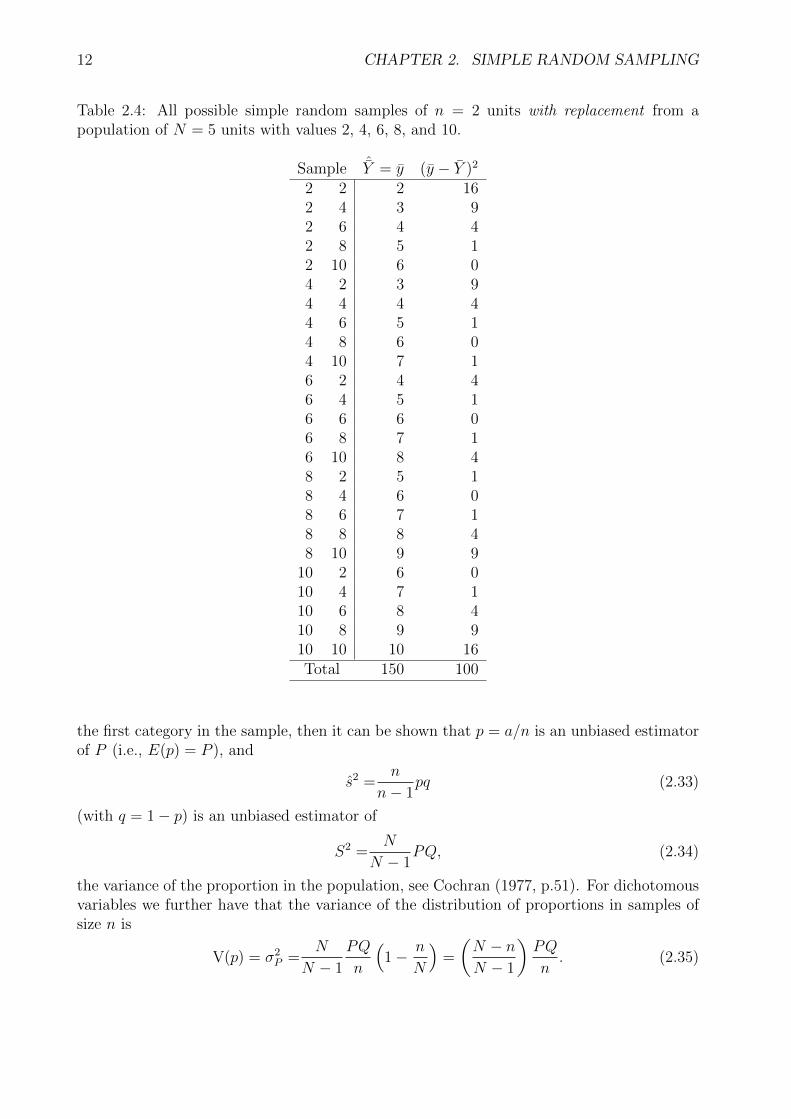
From this population we can draw a total of M = Nn = 52 = 25 different simple randomsamples of n = 2 units with replacement. For each sample we calculate its mean y, seeTable 2.4.
From Table 2.4 we see that
E(y) =1
M
M∑j=1
yj =1
25
25∑j=1
yj =150
25= 6,
which illustrates that the mean of the sample is still an unbiased estimator of the mean ofthe population when drawing simple random samples with replacement. Moreover, it followsfrom Table 2.4 that
σ2y =
1
M
M∑j=1
(yj − Y )2 =1
25
25∑j=1
(yj − 6)2 =100
25= 4,
and from (2.32) that – in this example –
V(y) = σ2y =
S2
n
(N − 1)
N=
(10
2
)(4
5
)= 4,
confirming that (2.32) indeed yields an unbiased estimate of the variance of the samplingdistribution of the mean when drawing simple random samples with replacement.
2.6 Unbiased estimators of proportions
When dealing with dichotomous (qualitative) variables with only two categories with Aunits in the population belonging to the first category and N − A in the population unitsbelonging to the second category, we have a proportion of P = A/N in the first category anda proportion of Q = 1− P in the second category. Letting a denote the number of units in
12 CHAPTER 2. SIMPLE RANDOM SAMPLING
Table 2.4: All possible simple random samples of n = 2 units with replacement from apopulation of N = 5 units with values 2, 4, 6, 8, and 10.
Sample ˆY = y (y − Y )2
2 2 2 162 4 3 92 6 4 42 8 5 12 10 6 04 2 3 94 4 4 44 6 5 14 8 6 04 10 7 16 2 4 46 4 5 16 6 6 06 8 7 16 10 8 48 2 5 18 4 6 08 6 7 18 8 8 48 10 9 9
10 2 6 010 4 7 110 6 8 410 8 9 910 10 10 16Total 150 100
the first category in the sample, then it can be shown that p = a/n is an unbiased estimatorof P (i.e., E(p) = P ), and
s2 =n
n− 1pq (2.33)
(with q = 1− p) is an unbiased estimator of
S2 =N
N − 1PQ, (2.34)
the variance of the proportion in the population, see Cochran (1977, p.51). For dichotomousvariables we further have that the variance of the distribution of proportions in samples ofsize n is
V(p) = σ2P =
N
N − 1
PQ
n
(1− n
N
)=
(N − nN − 1
)PQ
n. (2.35)
2.6. UNBIASED ESTIMATORS OF PROPORTIONS 13
If p and P are the sample and population percentages, respectively, falling into class C,(2.35) continues to hold for the variance of p. The square root of the latter variance is thestandard error of a proportion, and is denoted by σP . For populations that are not too small(say N > 20), the ratio N/(N − 1) in (2.35) may be dropped yielding
V(p) = σ2P =
PQ
n
(1− n
N
). (2.36)
Moreover, if the sampling fraction is also not too large (say n < 0.1N), then the latterformula can be further simplified to the well-known expression:
V(p) = σ2P =
PQ
n, (2.37)
see Moors and Muilwijk (1975, p.19). An unbiased estimator of the latter variance from thesample is obtained with:
v(p) = estimated σ2P = s2
y =s2
n
N − nN
= s2p =
pq
n− 1
(1− n
N
), (2.38)
compare with (2.28). It follows that if N is very large relative to n, so that the finitepopulation correction is negligible, an unbiased estimate of the variance of p is
v(p) = s2p =
pq
n− 1,
see Cochran (1977, p.51-52).
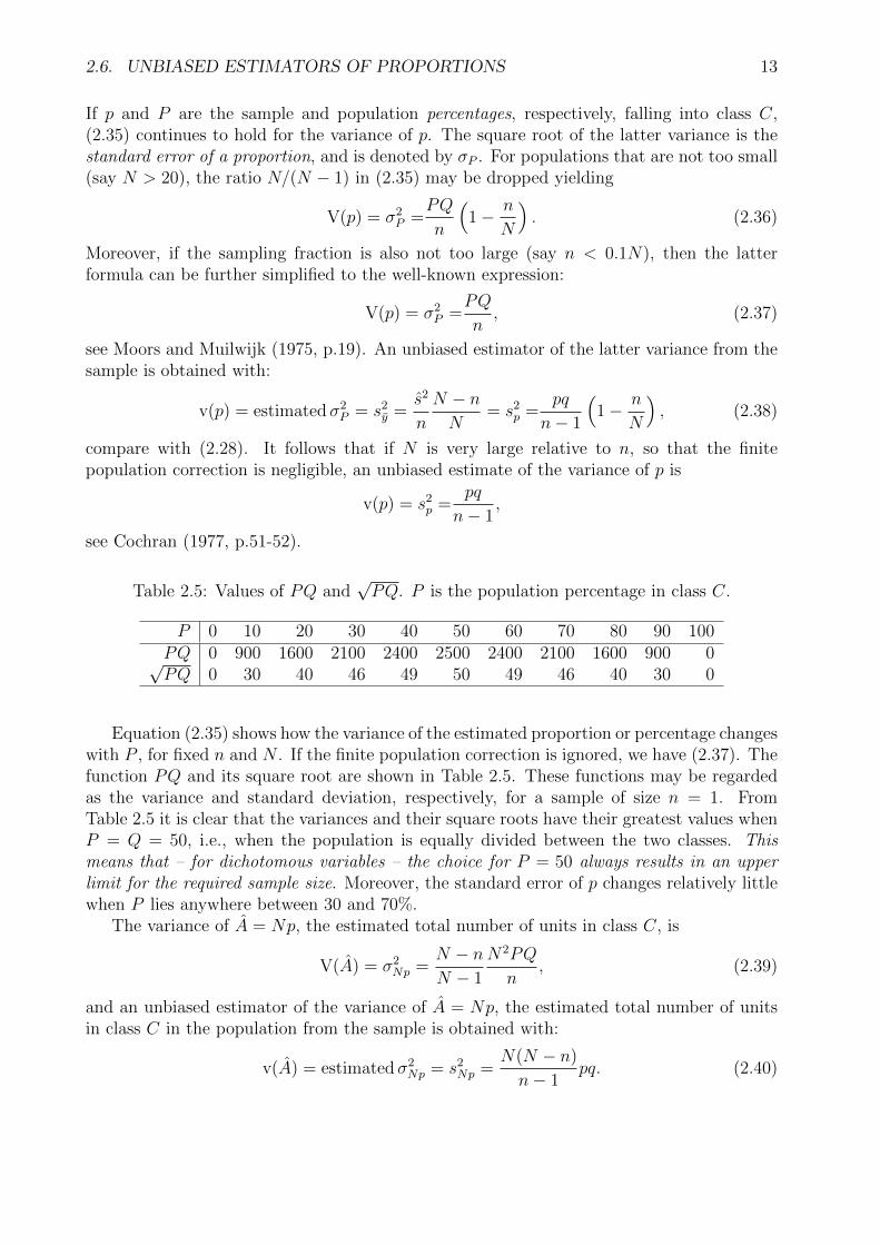
Table 2.5: Values of PQ and√PQ. P is the population percentage in class C.
P 0 10 20 30 40 50 60 70 80 90 100PQ 0 900 1600 2100 2400 2500 2400 2100 1600 900 0√PQ 0 30 40 46 49 50 49 46 40 30 0
Equation (2.35) shows how the variance of the estimated proportion or percentage changeswith P , for fixed n and N . If the finite population correction is ignored, we have (2.37). Thefunction PQ and its square root are shown in Table 2.5. These functions may be regardedas the variance and standard deviation, respectively, for a sample of size n = 1. FromTable 2.5 it is clear that the variances and their square roots have their greatest values whenP = Q = 50, i.e., when the population is equally divided between the two classes. Thismeans that – for dichotomous variables – the choice for P = 50 always results in an upperlimit for the required sample size. Moreover, the standard error of p changes relatively littlewhen P lies anywhere between 30 and 70%.
The variance of A = Np, the estimated total number of units in class C, is
V(A) = σ2Np =
N − nN − 1
N2PQ
n, (2.39)
and an unbiased estimator of the variance of A = Np, the estimated total number of unitsin class C in the population from the sample is obtained with:
v(A) = estimated σ2Np = s2
Np =N(N − n)
n− 1pq. (2.40)

14 CHAPTER 2. SIMPLE RANDOM SAMPLING
2.7 Confidence intervals
For large enough samples it can be assumed that the estimates of the mean y and the totalY are normally distributed about the population values µ = Y and Nµ = Y respectively,and confidence intervals for these estimates can be constructed as follows. For the mean Ywe have
y − tsy ≤ Y ≤ y + tsy, (2.41)
where sy is defined in (2.30) and t is the value of the normal deviate corresponding to thedesired confidence probability if n ≥ 50, and t is the value in the Student t table with (n−1)degrees of freedom if n < 50. For small samples with very skew distributions, however,special methods are needed.
For large enough samples, the value of the normal deviate corresponding to the 95%confidence probability is t = 1.96, and (2.41) equals
y − 1.96sy ≤ Y ≤ y + 1.96sy. (2.42)
Formula (2.42) expresses that the inequality holds with a confidence of 95%. On average,for 95 out of 100 samples the confidence interval will contain the actual population mean.The lower and upper limits calculated for a specific sample are called the 95% confidencelimits of the population mean, and the maximum distance of 1.96sy between the sample andthe population mean is called the 95% confidence interval. The ratio 1.96sy
yis known as the
relative confidence interval; it is 1.96 times the variation coefficient of y.For a qualitative variable, the confidence interval is
p− tsp ≤ P ≤ p+ tsp, (2.43)
where sp is the square root of (2.38).For the total Y the confidence interval is calculated as
Ny − tsY ≤ Y ≤ Ny + tsY , (2.44)
where sY is defined in (2.31). See Cochran (1977, p.27) and Hays (1970, Chapter 10).
Example 2-4. Signatures to a petition were collected on N = 676 sheets. Each sheethad enough space for 42 signatures, but on many sheets a smaller number of signatures hadbeen collected. The number of signatures per sheet were counted on a random sample ofn = 50 sheets (about 7% of the sample), with the results shown in Table 2.6. Estimate thetotal number of signatures to the petition and the 80% confidence limits.
Answer. Since the average number of signatures in this sample of 50 sheets is equal to
y =
∑19i=1 fiyi∑19i=1 fi
=(23)(42) + (4)(41) + · · ·+ (1)(3)
23 + 4 + · · ·+ 1=
1471
50= 29.42
signatures per sheet, the estimated total number of signatures in the population of 676 sheetsequals
y = Ny = (676)(29.42) = 19887.92.

2.8. ESTIMATION OF SAMPLE SIZE 15
Table 2.6: Results for a sample of 50 petition sheets: yi is the number of signatures, and fithe frequency of the number of sheets in the sample with yi signatures.
yi 42 41 36 32 29 27 23 19 16 15fi 23 4 1 1 1 2 1 1 2 2yi 14 11 10 9 7 6 5 4 3fi 1 1 1 1 1 3 2 1 1
An unbiased estimate of the variance of the population is obtained from (2.21), i.e., from
s2 =
∑19i=1(fi(yi − y))2
n− 1=
∑19i=1(fi(yi − y))2
49=
11220.18
49= 228.9832653,
with standard deviation
s =√s2 =
√228.9832653 = 15.13219301,
see (2.22). According to (2.31) the standard error of the total then equals
sY =Ns√n
√1− f =
(676)(15.13219301)√50
√1− 50
676= 1392.122281.
The 80% confidence limits of the total are therefore
Ny − 1.28sY ≤ Y ≤ Ny + 1.28sY ,
and thus
19887.92− (1.28)(1392.122281) ≤ Y ≤ 19887.92 + (1.28)(1392.122281),
meaning that
18106.00348 ≤ Y ≤ 21669.83652
with a confidence of 80%, i.e., in four out of five samples.
2.8 Estimation of sample size
As sample size increases, the distribution of the means of simple random samples from thesame population approaches the normal distribution more and more, irrespective whether thevariable of interest in the population is normally distributed or not. This is – loosely stated– the famous central limit theorem in statistics. In that case the mean y in the sample willtherefore be located between µ− 1.96σy and µ+ 1.96σy with a 95% probability, i.e.,
µ− 1.96σy ≤ y ≤ µ+ 1.96σy, (2.45)

16 CHAPTER 2. SIMPLE RANDOM SAMPLING
with a probability of 95%. It follows from (2.45) that
y − 1.96σy ≤ µ ≤ y + 1.96σy (2.46)
with the same probability. Substraction of y from (2.46) gives
−1.96σy ≤ µ− y ≤ +1.96σy (2.47)
and therefore
|µ− y| ≤ 1.96σy (2.48)
with a 95% probability.Substituting (2.25) in (2.48) we see that – for a continuous variable –
|µ− y| ≤ 1.96
√S2
n
(N − nN
)(2.49)
with a 95% probability. Assuming that we want the absolute error in our sample estimate yof the population mean µ to be no larger than d = |µ− y|, say, with a 95% probability, thenfrom the latter equation we can obtain a formula for the required minimal sample size n:
d = t
√S2
n
(N − nN
), (2.50)
Note that we have replaced the value 1.96 corresponding to a probability of 95% with t in(2.50) in order to be as general as possible. If we want a 95% probability then t = 1.96; fora 90% probability t = 1.64, for a 99% probability t = 2.58, et cetera. Solving (2.50) for nwe find that the minimal sample size should be
n =t2S2
t2S2
N+ d2
. (2.51)
For very large N this formula simplifies into
n0 =t2S2
d2, (2.52)
and we only need to estimate S. In this case it should be checked whether n0 < 0.1N . Ifnot we should apply the finite population correction and use
n =n0
1 + n0
N
, (2.53)
which is identical to (2.51), as it is not very difficult to verify.In order to establish the value of S in the population sometimes a small pilot study is
done. Or reasonable estimates can be found from previous studies in the same research field,from studies in similar research fields, or based on theoretical grounds. Even with a roughestimation we can thus obtain a useful indication about the required sample size. Note thatthe formulas in this section are based on the normal distribution. It should therefore be

2.8. ESTIMATION OF SAMPLE SIZE 17
checked that the estimated n is large enough. If not, a larger sample should be taken thenwas calculated.
So far formulas have been provided for the estimation of sample size based on the absoluteerror d = |µ− y| in the estimation of µ. If a relative error of the estimate of µ is used then
dY = tσy, (2.54)
or, upon substitution of (2.24),
dY = t
√S2
n
(N − nN
). (2.55)
In this case, d is a number satisfying 0 < d < 1. Solving (2.55) for n, we obtain
n =t2S2
t2S2
N+ d2Y 2
.
The latter formula can also be written as
n =
(tSdY
)2
1 + 1N
(tSdY
)2 , (2.56)
see Cochran (1977, p.77). For very large N this formula simplifies into
n0 =t2S2
d2Y 2. (2.57)
The required sample size can also be expressed in terms of the coefficient of variation c = SY
.Substitution of S = cY in (2.56) yields
n =t2c2
t2c2
N+ d2
. (2.58)
Example 2-5. For a bed of silver maple seedlings 1 ft wide and 430 ft long, it was foundby complete enumeration that µ = Y = 19 and S2 = 85.6, these being the true populationvalues. The sampling unit was 1 ft of the length of the bed, so that N = 430. With simplerandom sampling, how many units must be taken to estimate µ within 10% of accuracy,apart from a chance of 1 in 20?
Answer. Using (2.57) as a first approximation, and since dY = (0.1)(19) = 1.9 andt = 1.96, we obtain
n0 =(1.962)(85.6)
1.92= 91.09.
However, since n0/N = 91.09/430 = 0.21 is not negligible, we use (2.53) yielding
n =n0
1 + n0
N
=91.09
1.21= 75.28.

18 CHAPTER 2. SIMPLE RANDOM SAMPLING
Since 100(75.28/430) = 17.5, almost 18% of the bed has to be counted in order to attain theprecision desired.
For the estimation of sample size based on the absolute error d = |Nµ−Ny| of the totalNµ = Y in the population we have that
d = tσY , (2.59)
or, upon substitution of (2.26),
d = t
√N2S2
n
(N − nN
). (2.60)
Solving (2.60) for n, we obtain
n =t2S2
t2S2
N+ d2
N2
. (2.61)
If the finite population correction is negligible, i.e., if n < 0.1N , then the latter formulasimplifies into
n0 =t2N2S2
d2. (2.62)
If an estimation of the sample size is required based on the relative error dNY of thetotal Nµ = Y , where 0 < d < 1, we need to solve
dNY = t
√N2S2
n
(N − nN
), (2.63)
yielding for n
n =t2S2
t2S2
N+ d2Y 2
. (2.64)
For large N the latter formula simplifies into
n0 =t2S2
d2Y 2. (2.65)
Example 2-6. In a certain year we have a population of N = 7 million car driversin a country. On average these road users drive Y = 15, 000 kilometers that year, with astandard deviation of S = 5, 000 kilometers. The total amount of kilometers driven by cardrivers that year is therefore NY = 105 billion kilometers. With simple random sampling,how many drivers must be selected to estimate the latter total NY within 5% of accuracy,apart from a chance of 1 in 20?
2.8. ESTIMATION OF SAMPLE SIZE 19
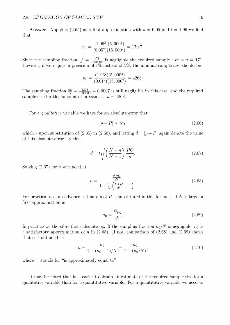
Answer. Applying (2.65) as a first approximation with d = 0.05 and t = 1.96 we findthat
n0 =(1.962)(5, 0002)
(0.052)(15, 0002)= 170.7.
Since the sampling fraction n0
N= 171
7000000is negligible the required sample size is n = 171.
However, if we require a precision of 1% instead of 5%, the minimal sample size should be
n0 =(1.962)(5, 0002)
(0.012)(15, 0002)= 4268.
The sampling fraction n0
N= 4268
7000000= 0.0007 is still negligible in this case, and the required
sample size for this amount of precision is n = 4268.
For a qualitative variable we have for an absolute error that
|p− P | ≤ tσP (2.66)
which – upon substitution of (2.35) in (2.66), and letting d = |p−P | again denote the valueof this absolute error – yields
d = t
√(N − nN − 1
)PQ
n. (2.67)
Solving (2.67) for n we find that
n =t2PQd2
1 + 1N
(t2PQd2 − 1
) . (2.68)
For practical use, an advance estimate p of P is substituted in this formula. If N is large, afirst approximation is
n0 =t2pq
d2. (2.69)
In practice we therefore first calculate n0. If the sampling fraction n0/N is negligible, n0 isa satisfactory approximation of n in (2.68). If not, comparison of (2.68) and (2.69) showsthat n is obtained as
n =n0
1 + (n0 − 1)/N.=
n0
1 + (n0/N), (2.70)
where.= stands for “is approximately equal to”.
It may be noted that it is easier to obtain an estimate of the required sample size for aqualitative variable than for a quantitative variable. For a quantitative variable we need to

20 CHAPTER 2. SIMPLE RANDOM SAMPLING
have an estimate of the variance S2 of the variable in the population if we use an absoluteerror, see (2.51) and (2.61), and estimates of both of the mean Y and the variance S2 of thevariable in the population if we use a relative error, see (2.56) and (2.64). For a qualitativevariable, on the other hand, we only need an estimate of the proportion or percentage P inthe population, see (2.68). Even if we do not know this proportion or percentage, it is stillpossible to obtain an estimate of the required sample size by using a value of P = 0.5 in(2.68), since this yields an upper bound for the required sample size (see also Section 2.6).
Example 2-7. An anthropologist is preparing to study the inhabitants of some island.Among other things, he wishes to estimate the percentage of inhabitants belonging to bloodgroup O. The anthropologist wants this percentage to be correct within 5% in the sense that,if the sample shows 43% to have blood group O, the percentage for the whole island is sureto lie within 38% and 48%. He also is willing to take a 1 in 20 chance of getting an unluckysample. The total population of the island is N = 3200. How large should the sample be?
Answer. In technical terms, the proportion p from the sample is to lie in the range P±5,except for a 1 in 20 chance. Thus, d = |p − P | = 0.05 in (2.68), and t = 1.96. Moreover,assuming the worst case scenario where P = 0.5 (see Section 2.6), it follows from (2.69) that– as a first approximation – the sample size should be
n0 =1.962(0.5)(0.5)
0.052=
0.9604
0.0025= 384.2.
Since n0/N = 384/3200 = 0.12, which is larger than 0.1, the finite population correction(fpc) is needed. Correcting for the fpc by application of (2.70) results in an estimated samplesize of
n =384
1 + (384− 1)/3200= 343.
Example 2-8. For the same population as in Example 2-6 we wish to estimate thepercentage of car drivers wearing their seat belt. We want this percentage to be correctwithin 5% in the sense that, if the sample shows 80% to wear a seat belt, the percentage forthe whole car driver population is sure to lie within 75% and 85%. We also are willing totake a 1 in 20 chance of getting an unlucky sample. How large should this sample be?
Answer. The proportion p from the sample is to lie in the range P ± 0.05, except for a1 in 20 chance. Thus, d = |p − P | = 0.05 in (2.68), and t = 1.96. Moreover, assuming theworst case scenario where P = 0.5 (see Section 2.6), it follows from (2.69) that – as a firstapproximation – the sample size should be
n0 =1.962(0.5)(0.5)
0.052=
0.49
0.0025= 384.2.
Since n0/N = 384/5, 000, 000.= 0, the finite population correction (fpc) is not needed.
Assuming that P = 0.8 in the population we obtain
n0 =1.962(0.8)(0.2)
0.052=
2.4586
0.0025= 246.

2.9. SAMPLE SIZE WITH MORE THAN ONE ITEM 21
Again assuming P = 0.8, but now requiring a precision of 1% instead of 5% we have
n0 =1.962(0.8)(0.2)
0.012=
0.614656
0.0001= 6, 147,
where the fpc is still not needed.
Sometimes, particularly when estimating the total number NP of units in class C, wewish to control the relative error instead of the absolute error in Np; for example, we maywish to estimate NP with an error not exceeding 10%. Then
dP = tσP , (2.71)
or, upon substitution of (2.35),
dP = t
√PQ
n
(N − nN − 1
). (2.72)
In this case, d is again a number satisfying 0 < d < 1. For this specification, replace d bydP in formulas (2.68) and (2.69). From (2.69) we then get
n0 =t2pq
d2p2=t2
d2
q
p, (2.73)
while formula (2.70) is unchanged.We end by noting that the value of d in formulas (2.50), (2.55), (2.60), (2.67), (2.71) is
known as the sampling error. For given population variance S2, population mean Y , and/orpopulation proportion P , whichever is appropriate, and population size N , sample size n,and confidence limit t, these formulas can therefore also be used to calculate the samplingerror of a particular sampling design.
Example 2-9. From a population of 10, 000 car drivers with a percentage of 80 wearingthe seat belt, a simple random sample of 400 car drivers is drawn. Assuming a 1 in 20 chanceof getting an unlucky sample, what is the sampling error of this sample?
Answer. Since N = 10, 000, P = 0.8, n = 400, and t = 1.96 in this situation, we apply(2.67) which gives
d = t
√(N − nN − 1
)PQ
n= 1.96
√(10, 000− 400
10, 000− 1
)(0.8)(0.2)
400= 0.048.
The absolute sampling error in this sampling design is therefore 4.8%.
2.9 Sample size with more than one item
In many surveys information has to be collected on more than one item. One method ofdetermining sample size is to select those items that are considered the most vital, and then

22 CHAPTER 2. SIMPLE RANDOM SAMPLING
to estimate the minimal sample size needed for each of these vital items separately. Whenthe single item estimations of n have been completed, it is time to make decisions based onthe results. If the estimations are all reasonably close, and the largest n is within budget,then this sample size is used. When the n’s are quite different, however, selecting the largestn may result in an overall precision that is much higher than originally intended, or in avery expensive survey. In this case, the desired precision may be lowered for some items thusallowing for the use of a smaller sample size. Sometimes the estimated n’s vary so wildlythat items simply have to be dropped from the survey altogether in view of the resourcesavailable and the precision required for the purpose of the survey.
Example 2-10. Again consider Examples 2-6 and 2-8, where it was found – using simplerandom sampling – that the estimation of the total distance traveled by car drivers with aprecision of 1% required a minimal sample size of n = 4, 268 car drivers, while the estimationof the total percentage of seat belt wearing by the same population with a precision of 1%required a minimal sample size of n = 6, 147 car drivers. If we want to obtain estimates forboth these items with a precision of 1%, we therefore should select a simple random sampleof n = 6, 147 car drivers.
2.10 Sample size when estimates are needed for sub-
populations
In Section 2.6 we discussed how to obtain an unbiased estimate of the number of units inthe population having a certain property. It often happens that the category is so importantthat we are not only interested in its size but also in the mean or total of the variable ofinterest in this category. Such categories are also known as subpopulations or domains ofstudy.
Consider a population of N units, of which A units belong to a certain subpopulation.We will denote parameters corresponding to this subpopulation with the subscript s, and Ystherefore refers to the total of variable y in the subpopulation, and Ys to its mean. Then
Ys =A∑i=1
yi and Ys =1
A
A∑i=1
yi, (2.74)
are the subtotal and the submean of the population, respectively, and – letting a denote thenumber of elements in a random sample of this subpopulation –
ys =1
a
a∑i=1
yi (2.75)
is an unbiased estimator of the submean of the population. The variance of y in the sub-population is
S2s =
1
A− 1
A∑i=1
(yi − Ys)2, (2.76)

2.10. SAMPLE SIZE WHEN ESTIMATES ARE NEEDED FOR SUBPOPULATIONS 23
and an unbiased sample estimator of this variance is
s2s =
1
a− 1
a∑i=1
(yi − ys)2, (2.77)
compare with (2.21).Formulas (2.24) and (2.28) for the variance of the mean and the sample estimator of the
variance of the mean still apply to subpopulations, in which case they can be written as
V(ys) = σ2ys =
S2s
a(1− a
A), (2.78)
and
v(ys) = estimated σ2ys = s2
ys =s2s
a(1− a
A), (2.79)
respectively. Analogous to (2.41), confidence limits for the sample estimate of the submean(2.75) can be constructed with
ys − tsys ≤ Ys ≤ ys + tsys , (2.80)
where sys is the square root of (2.79) and t is again the value of the normal deviate corre-sponding to the desired confidence probability if n ≥ 50, and the value in the Student t tablewith (n− 1) degrees of freedom if n < 50. For the finite population correction in (2.78) and(2.79), 1− n
Ncan be used instead of 1− a
Awhen A is unknown. For unknown A, therefore,
formulas (2.78) and (2.79) turn into
V(ys) = σ2ys =
S2s
a(1− n
N), (2.81)
and
v(ys) = estimated σ2ys = s2
ys =s2s
a(1− n
N), (2.82)
respectively.As far as the estimation of the subtotal is concerned, no problems arise as long as the
size A of the subpopulation is known. An unbiased estimator of the total is then
Ays =A
a
a∑i=1
yi, (2.83)
and all the results in Sections 2.4 and 2.7 apply again. So formulas (2.26) and (2.29) forthe variance of the total and the sample estimator of the variance of the total also apply tosubpopulations, in which case they can be written as
V(Ys) = σ2Ys
=A2S2
s
a(1− a
A), (2.84)
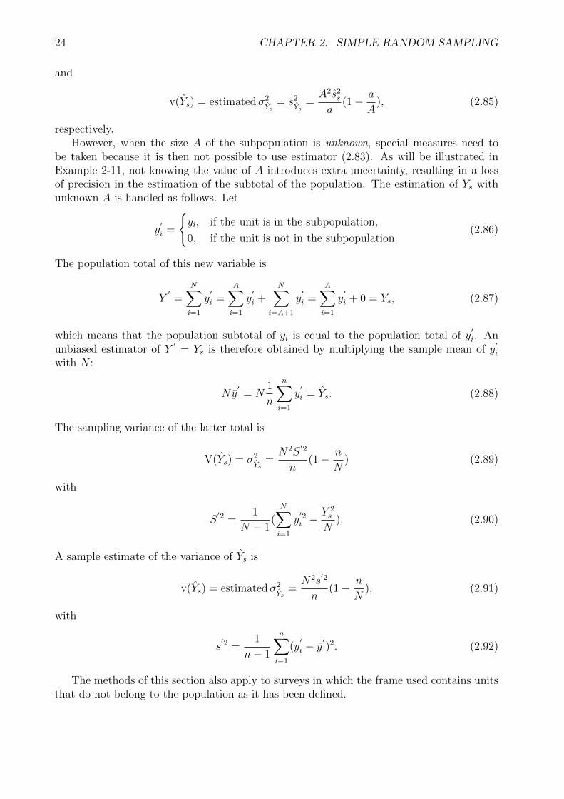
24 CHAPTER 2. SIMPLE RANDOM SAMPLING
and
v(Ys) = estimated σ2Ys
= s2Ys
=A2s2
s
a(1− a
A), (2.85)
respectively.However, when the size A of the subpopulation is unknown, special measures need to
be taken because it is then not possible to use estimator (2.83). As will be illustrated inExample 2-11, not knowing the value of A introduces extra uncertainty, resulting in a lossof precision in the estimation of the subtotal of the population. The estimation of Ys withunknown A is handled as follows. Let
y′
i =
{yi, if the unit is in the subpopulation,
0, if the unit is not in the subpopulation.(2.86)
The population total of this new variable is
Y′=
N∑i=1
y′
i =A∑i=1
y′
i +N∑
i=A+1
y′
i =A∑i=1
y′
i + 0 = Ys, (2.87)
which means that the population subtotal of yi is equal to the population total of y′i. An
unbiased estimator of Y′
= Ys is therefore obtained by multiplying the sample mean of y′i
with N :
Ny′
= N1
n
n∑i=1
y′
i = Ys. (2.88)
The sampling variance of the latter total is
V(Ys) = σ2Ys
=N2S
′2
n(1− n
N) (2.89)
with
S′2 =
1
N − 1(N∑i=1
y′2i −
Y 2s
N). (2.90)
A sample estimate of the variance of Ys is
v(Ys) = estimated σ2Ys
=N2s
′2
n(1− n
N), (2.91)
with
s′2 =
1
n− 1
n∑i=1
(y′
i − y′)2. (2.92)
The methods of this section also apply to surveys in which the frame used contains unitsthat do not belong to the population as it has been defined.

2.10. SAMPLE SIZE WHEN ESTIMATES ARE NEEDED FOR SUBPOPULATIONS 25
Example 2-11. The number of children living with their parents is determined in asimple random sample of n = 200 families from a large population consisting of 2.6 millionfamilies, meaning that the finite population correction may be ignored. The frequencydistribution of the number of children in the sample is shown in Table 2.7. First estimate theaverage number of children per family in the total population, including its 95% confidenceinterval. Next estimate the average number of children in families with at least four children,and its standard error. Finally estimate the total number of children and its standard errorin families with at least four children, in the following two situations: 1) the total numberof families with four or more children in the population is known, and 2) this total numberis unknown.
Table 2.7: Number of children in a simple random sample of 200 families.
Number of children Frequencyyj fj fjyj fjy
2j
0 62 0 01 51 51 512 39 78 1563 22 66 1984 12 48 1925 7 35 1756 4 24 1448 2 16 128
10 1 10 100Total 200 328 1144
Answers. Let k = 9 denote the total number of categories in the frequency distributionof Table 2.7. Then an unbiased estimate of the average number of children per family in thepopulation is
y =
∑ni=1 yin
=
∑kj=1 fjyj∑kj=1 fj
=328
200= 1.64.
An unbiased estimate of the variance in the population is
s2 =
∑ni=1(yi − y)2
n− 1=
∑kj=1 fjy
2j −
(∑k
j=1 fjyj)2∑kj=1 fj
(∑k
j=1 fj)− 1=
1144− (328)2
200
199= 3.0456,
and the estimated standard error of the mean therefore equals
sy =
√s2
n=
√3.0456
200= 0.1234.
The 95% upper and lower confidence limits of the mean are y−1.96sy = 1.64−(1.96)(0.1234) =1.398 and y + 1.96sy = 1.64 + (1.96)(0.1234) = 1.882, respectively.

26 CHAPTER 2. SIMPLE RANDOM SAMPLING
Letting the index j only refer to the categories 4 through 10 in Table 2.7, an unbiasedestimate of the submean of families with at least four children is
ys =1
a
a∑i=1
yi =
∑kj=1 yj∑kj=1 fj
=133
26= 5.12.
An unbiased sample estimate of the variance of the latter submean equals
s2s =
1
a− 1
a∑i=1
(yi − ys)2 =
∑fjy
2j −
(∑fjyj)2∑fj
(∑fj)− 1
=739− (133)2
26
26− 1= 2.3462,
see (2.77), meaning that the sample estimate of the standard error of this submean is
sys =
√s2s
a=
√2.3462
26= 0.3004.
We next show how to estimate the subtotal number of children in families with four ormore children – and its standard error –, in the situation that the total number A of familieswith four or more children in the population is known, based on the sample data in Table 2.7.
When the size A of the subpopulation of families with four or more children is known,sample estimates of the subtotal and its standard error are obtained with (2.83) and (2.85),yielding (A)(5.12) and (A)(0.3004) in the present situation, respectively. The coefficient ofvariation of this estimate of the subtotal is therefore Asys
Ays= 0.3004
5.12= 0.0587.
When A is unknown, an estimate of the subtotal is calculated with (2.88) yielding
Ys = Ny′= N
1
n
n∑i=1
y′
i = (2.6)(1
200)(133) = 1.729 million.
The standard error of the latter subtotal is found with (2.91), which requires the calculationof (2.92):
s′2 =
1
n− 1
n∑i=1
(y′ − y′
)2 =
∑kj=1 fjy
′2j −
(∑k
j=1 fjy′j)2∑k
j=1 fj
(∑k
j=1 fj)− 1=
739− 1332
200
199= 3.269.
Note that the index j in the latter formula now again runs over all nine categories of thevariable in Table 2.7. But the values of yj corresponding to the categories 0 through 3 (notbeing part of the subpopulation of families of four children or more) are all set equal to zeroin this case. The standard error of the subtotal therefore equals
sYs =
√N2s′2
n=Ns
′
√n
=2.6√
3.269√200
= 0.333.
When A is unknown, the coefficient of variation of the estimate equalssYsYs
= 0.3333.269
= 0.19.
This is a more than three-fold increase compared with the coefficient of variation of 0.0587when the size A of the population is known, which illustrates the increased uncertainty thatis introduced in the estimation of subtotals when the size of the subpopulation of interest isnot known.

2.10. SAMPLE SIZE WHEN ESTIMATES ARE NEEDED FOR SUBPOPULATIONS 27
We end this section by discussing how to estimate sample size n in simple random sam-pling when precision requirements are not only imposed on parameter estimates of the popu-lation of interest, but also on parameter estimates of a subpopulation. We again distinguishtwo situations: one where A – the size of the subpopulation – is known, and the other whereA is unknown.
For an absolute error of the submean no larger than d = |Ys− ys| , the minimum samplesize is determined by
d = tσYs , (2.93)
where t is the value of the normal deviate corresponding to the desired confidence probability,as before. When A is known, formula (2.78) for σYs can be substituted in (2.93), yielding
d = t
√S2s
a(1− a
A). (2.94)
Solving (2.94) with respect to a gives
a =t2S2
s
d2 + 1At2S2
s
. (2.95)
The minimal sample size n is then obtained from
n =aN
A. (2.96)
When A is unknown, formula (2.81) is substituted in (2.93) which results in
d = t
√S2s
a(1− n
N). (2.97)
In this case we have one equation with two unknowns: a and n. This is solved by making aguess, say Ag, about the size of the subpopulation, and then substituting the expected value
of a = Agn
Nin (2.96). Solving the result with respect to n yields
n =t2S2
sN
Agd2 + t2S2s
. (2.98)
When in doubt, a value for Ag should be chosen that is as small as reasonably possible, sincethe sample size n will then be on the safe side.
Similar derivations apply for the derivation of minimal sample size in the estimation ofsubtotals in simple random sampling.

28 CHAPTER 2. SIMPLE RANDOM SAMPLING

Chapter 3
Stratified random sampling
3.1 Introduction
Simple random sampling as discussed in the previous chapter is not necessarily the mostefficient sampling strategy. One possible way to improve precision in the parameter estimatesof the population – and thus to reduce the required sample size for their estimation – is todivide the population of size N into a number of mutually exclusive sub-populations of sizesN1, N2, . . . , NL such that
N = N1 +N2 + · · ·+NL,
and then to apply simple random sampling to each of these L sub-populations separately.These mutually exclusive sub-populations (e.g., males and females) are called strata. Thesample sizes in the strata are denoted by n1, n2, . . . , nL, respectively. This sampling proce-dure is called stratified random sampling.
Generally, with stratified random sampling considerable gains in precision of the estimatesor considerable reduction in costs can be obtained when the population variance of thevariable of interest is (much) smaller within each stratum than in the total population.Examples of such situations will be provided below. Since most guidelines can be given forthis situation, the largest part of this chapter is devoted to this case.
However, other important reasons for using stratification can also be:
• The population of interest is registered in more than one sampling frame. If theseframes are located in different places one is almost forced to draw separate samplesfrom the corresponding parts of the population.
• The method of observation or of sampling or of estimation must be performed differ-ently in different parts of the population.
• If the survey requires precise estimates for certain subdivisions of the total population,it is advisable to treat these subdivisions as separate strata.
In Sections 3.2 through 3.9 we will first assume that the number and types of strata havealready been decided upon and constructed. The problem of how to construct the strataand of how many strata there should be is taken up in Section 3.10.
29
30 CHAPTER 3. STRATIFIED RANDOM SAMPLING
3.2 Properties of the parameter estimates
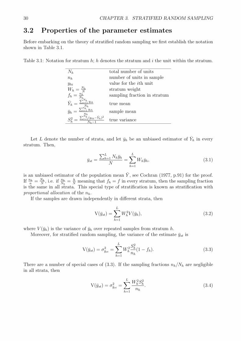
Before embarking on the theory of stratified random sampling we first establish the notationshown in Table 3.1.
Table 3.1: Notation for stratum h; h denotes the stratum and i the unit within the stratum.
Nh total number of unitsnh number of units in sampleyhi value for the ith unitWh = Nh
Nstratum weight
fh = nh
Nhsampling fraction in stratum
Yh =∑Nh
i=1 yihNh
true mean
yh =∑nh
i=1 yihnh
sample mean
S2h =
∑Nhi=1(yih−Yh)2
Nh−1true variance
Let L denote the number of strata, and let yh be an unbiased estimator of Yh in everystratum. Then,
yst =
∑Lh=1NhyhN
=L∑h=1
Whyh, (3.1)
is an unbiased estimator of the population mean Y , see Cochran (1977, p.91) for the proof.If nh
n= Nh
N, i.e. if nh
Nh= h
Nmeaning that fh = f in every stratum, then the sampling fraction
is the same in all strata. This special type of stratification is known as stratification withproportional allocation of the nh.
If the samples are drawn independently in different strata, then
V(yst) =L∑h=1
W 2hV (yh), (3.2)
where V (yh) is the variance of yh over repeated samples from stratum h.Moreover, for stratified random sampling, the variance of the estimate yst is
V(yst) = σ2yst =
L∑h=1
W 2h
S2h
nh(1− fh). (3.3)
There are a number of special cases of (3.3). If the sampling fractions nh/Nh are negligiblein all strata, then
V(yst) = σ2yst =
L∑h=1
W 2hS
2h
nh. (3.4)

3.2. PROPERTIES OF THE PARAMETER ESTIMATES 31
With proportional allocation we may substitute
nh =nNh
N
in (3.3) yielding
V(yst) = σ2yst =
1− fn
L∑h=1
WhS2h. (3.5)
Finally, if sampling is proportional and the variances in all strata have the same value, S2w,
(3.5) further simplifies into
V(yst) = σ2yst =
S2w
n(1− f). (3.6)
If Yst = Nyst is the estimate of the population total Y , then
V(Yst) = σ2Yst
=L∑h=1
Nh(Nh − nh)S2h
nh(3.7)
is the variance of the sampling distribution of the total Yst of the stratified population.
Example 3-1. Given is a hypothetical population consisting of N = 7 units with values3, 6, 6, 8 ,15, 18, and 28. For this population the total, the mean, and the variance are
Y =∑N
i=1 yi = 84, Y =∑N
i=1 yiN
= 847
= 12, and S2 =∑N
i=1(yi−Y )2
N−1= 470
6= 781
3, respectively.
Moreover, if we draw a simple random sample of n = 5 units from this population, then itfollows from (2.26) that the sampling variance of the total Y = Ny equals
V(Y ) = σ2Y
=N2S2
n(1− f) =
(72)(7813)
5(1− 5
7) = 219
1
3.
Now suppose that we divide this population into the two strata shown in Table 3.2.
Table 3.2: Population of N = 7 units divided into two strata of N1 = 4 and N2 = 3 units.
Stratum Values Total1 3 6 6 15 302 8 18 28 54
We first of all note that the population totals in the two strata are Y1 = 30 and Y2 =54, respectively, and that the corresponding population means are Y1 = 30
4= 7.5 and
Y2 = 543
= 18, respectively, so that the grand mean in the population is∑L
h=1WhYh =(4
7)(7.5) + (3
7)(18) = 12 = Y . The variances of the units within these two strata of the
population are S21 =
∑N1i=1(yi1−Y1)2
N1−1= 81
3= 27 and S2
2 =∑N2
i=1(yi2−Y2)2
N2−1= 200
2= 100, respectively.

32 CHAPTER 3. STRATIFIED RANDOM SAMPLING
We now draw a simple random sample of n1 = 3 units from stratum 1, and a simplerandom sample of n2 = 2 units from stratum 2. Since there are M = ΠL
h=1Nh!
nh!(Nh−nh)!
possible samples in stratified random sampling without replacement, we have a total ofM = ( N1!
n1!(N1−n1)!))( N2!n2!(N2−n2)!)
) = ( 4!3!1!
)( 3!2!1!
) = (4)(3) = 12 possible random samples in thepresent situation. All these 12 possible random samples are given in Table 3.3.
Table 3.3: All possible simple random samples of size n1 = 3 and n2 = 2 without replacementfrom the two population strata in Table 3.2, and their statistics.
Sample number Stratum 1 Stratum 2 y1 y2 Y1 Y2 Y1 3 6 6 8 18 5 13 20 39 592 3 6 6 8 28 5 18 20 54 743 3 6 6 18 18 5 23 20 69 894 3 6 15 8 28 8 13 32 39 715 3 6 15 8 28 8 18 32 54 866 3 6 15 18 28 8 23 32 69 1017 3 6 15 8 18 8 13 32 39 718 3 6 15 8 28 8 18 32 54 869 3 6 15 18 28 8 23 32 69 101
10 6 6 15 8 18 9 13 36 39 7511 6 6 15 8 28 9 18 36 54 9012 6 6 15 18 28 9 23 36 69 105
Total 90 216 360 648 1008Expectation= Total/12 7.5 18 30 54 84
A comparison of the expectations in Table 3.3 with the population parameters shows thatthe estimators are indeed unbiased, since E(yh) = Yh for h = 1, 2, E(Yh) = Yh for h = 1, 2,
E(Y ) = Y , and also E( ˆY ) = Y because 847
= 12.Moreover, from (3.7) we obtain the variance of the sampling distribution of the stratified
population total
V(Yst) =L∑h=1
Nh(Nh − nh)S2h
nh= N1(N1 − n1)
S21
n1
+N2(N2 − n2)S2
2
n2
(3.8)
=4(4− 3)27
3+ 3(3− 2)
100
2= (4)(9) + (3)(50) = 186.
For a simple random sample of n1 = 2 and n2 = 3 from stratum 1 and 2 in Table 3.2, onthe other hand, it follows from (3.7) that
V(Yst) =N1(N1 − n1)S2
1
n1
+N2(N2 − n2)S2
2
n2
(3.9)
=4(4− 2)27
2+ 3(3− 3)
100
3= (8)(
27
2) = (4)(27) = 108.
A summary of the results for this example are given in Table 3.4. As the latter tableclearly indicates, for a sample of n = 5 units drawn from a population of N = 7 units, the
3.2. PROPERTIES OF THE PARAMETER ESTIMATES 33
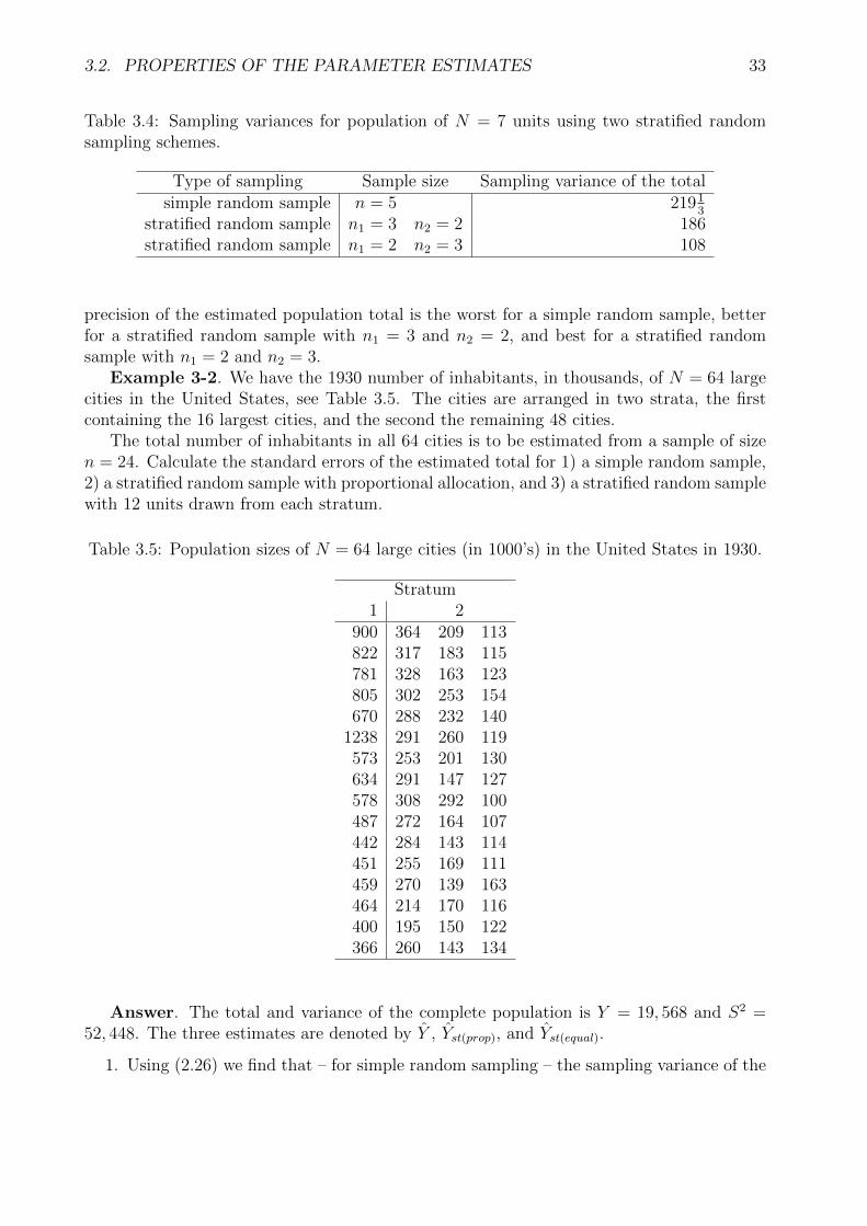
Table 3.4: Sampling variances for population of N = 7 units using two stratified randomsampling schemes.
Type of sampling Sample size Sampling variance of the totalsimple random sample n = 5 2191
3
stratified random sample n1 = 3 n2 = 2 186stratified random sample n1 = 2 n2 = 3 108
precision of the estimated population total is the worst for a simple random sample, betterfor a stratified random sample with n1 = 3 and n2 = 2, and best for a stratified randomsample with n1 = 2 and n2 = 3.
Example 3-2. We have the 1930 number of inhabitants, in thousands, of N = 64 largecities in the United States, see Table 3.5. The cities are arranged in two strata, the firstcontaining the 16 largest cities, and the second the remaining 48 cities.
The total number of inhabitants in all 64 cities is to be estimated from a sample of sizen = 24. Calculate the standard errors of the estimated total for 1) a simple random sample,2) a stratified random sample with proportional allocation, and 3) a stratified random samplewith 12 units drawn from each stratum.
Table 3.5: Population sizes of N = 64 large cities (in 1000’s) in the United States in 1930.
Stratum1 2
900 364 209 113822 317 183 115781 328 163 123805 302 253 154670 288 232 140
1238 291 260 119573 253 201 130634 291 147 127578 308 292 100487 272 164 107442 284 143 114451 255 169 111459 270 139 163464 214 170 116400 195 150 122366 260 143 134
Answer. The total and variance of the complete population is Y = 19, 568 and S2 =52, 448. The three estimates are denoted by Y , Yst(prop), and Yst(equal).
1. Using (2.26) we find that – for simple random sampling – the sampling variance of the

34 CHAPTER 3. STRATIFIED RANDOM SAMPLING
total Y equals
V(Y ) = σ2Y
=N2S2
n(1− f) =
(642)(52, 448)
24
(64− 24
24
)= 5, 594, 453,
with a standard error of σ(Y ) =√
5, 594, 453 = 2365.
2. The population variances in the two strata are S21 = 53, 843 and S2
2 = 5581, respec-tively. Note that the population variance of the 16 largest cities in the first stratumis almost ten times as large as the population variance of the 48 cities in the secondstratum. In proportional allocation we have n1 = 6 and n2 = 18, since n1
N1= n2
N2in this
case. Applying (3.7) to this situation we obtain
V(Yst(prop)) = σ2Yst(prop)
= N1(N1 − n1)S2
1
n1
+N2(N2 − n2)S2
2
n2
= 16(16− 6)53, 843
6+ 48(48− 18)
5581
18= 1, 882, 293.334,
from which it follows that the standard error σ(Yst(prop)) equals√
1, 882, 293.334 = 1372for proportional stratified random sampling.
3. Applying (3.7) to an equal allocation with n1 = n2 = 12 we find that
V(Yst(prop)) = σ2Yst(prop)
= N1(N1 − n1)S2
1
n1
+N2(N2 − n2)S2
2
n2
= 16(16− 12)53, 843
12+ 48(48− 12)
5581
12= 1, 090, 826.667,
meaning that the standard error σ(Yst(equals)) is√
1, 090, 826.667 = 1044 for stratifiedrandom sampling using equal allocation.
We end example 3-2 by noting that equal sample sizes in the two strata are more precisethan proportional allocation in this case, and that both stratified random sampling schemesare greatly superior to simple random sampling because the units in the two strata are muchmore homogeneous than the units in the complete population.
3.3 The estimated variances and confidence limits
It is clear from (2.21) in Section 2.3 that an unbiased estimator of the population variancein stratum h is
s2h =
1
nh − 1
nh∑i=1
(yhi − yh)2, (3.10)
if a simple random sample is taken within each stratum. This means that with stratifiedrandom sampling
v(yst) = estimated σ2yst = s2
yst =1
N2
L∑h=1
Nh(Nh − nh)s2h
nh, (3.11)
3.4. OPTIMUM ALLOCATION TO STRATA 35
is an unbiased estimator of the variance of yst, see Cochran (1977, p.95) for a proof.If yst is normally distributed, it follows from (3.11) that the confidence limits for the
population mean are equal to
yst ± tsyst , (3.12)
while those of the population total are
Nyst ± tNsyst , (3.13)
where t can be read from tables of the normal distribution.
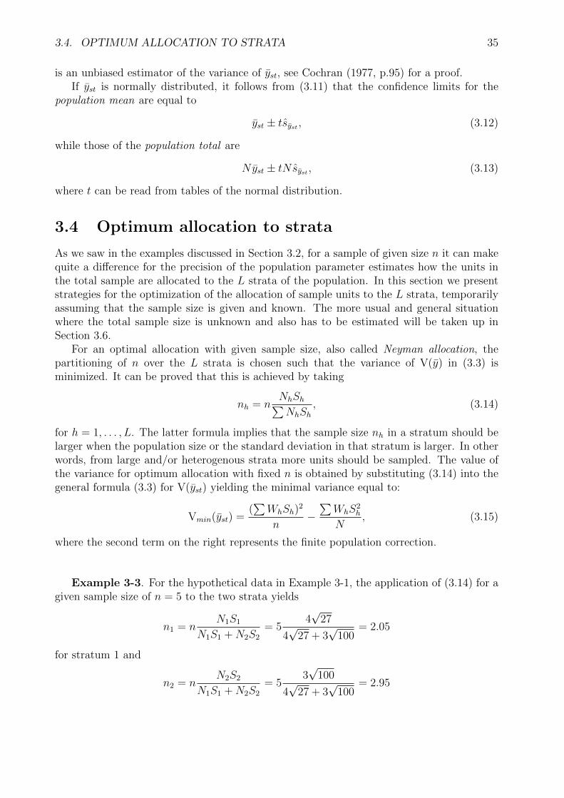
3.4 Optimum allocation to strata
As we saw in the examples discussed in Section 3.2, for a sample of given size n it can makequite a difference for the precision of the population parameter estimates how the units inthe total sample are allocated to the L strata of the population. In this section we presentstrategies for the optimization of the allocation of sample units to the L strata, temporarilyassuming that the sample size is given and known. The more usual and general situationwhere the total sample size is unknown and also has to be estimated will be taken up inSection 3.6.
For an optimal allocation with given sample size, also called Neyman allocation, thepartitioning of n over the L strata is chosen such that the variance of V(y) in (3.3) isminimized. It can be proved that this is achieved by taking
nh = nNhSh∑NhSh
, (3.14)
for h = 1, . . . , L. The latter formula implies that the sample size nh in a stratum should belarger when the population size or the standard deviation in that stratum is larger. In otherwords, from large and/or heterogenous strata more units should be sampled. The value ofthe variance for optimum allocation with fixed n is obtained by substituting (3.14) into thegeneral formula (3.3) for V(yst) yielding the minimal variance equal to:
Vmin(yst) =(∑WhSh)
2
n−∑WhS
2h
N, (3.15)
where the second term on the right represents the finite population correction.
Example 3-3. For the hypothetical data in Example 3-1, the application of (3.14) for agiven sample size of n = 5 to the two strata yields
n1 = nN1S1
N1S1 +N2S2
= 54√
27
4√
27 + 3√
100= 2.05
for stratum 1 and
n2 = nN2S2
N1S1 +N2S2
= 53√
100
4√
27 + 3√
100= 2.95

36 CHAPTER 3. STRATIFIED RANDOM SAMPLING
for stratum 2. Rounding these numbers the optimal allocation is n1 = 2 and n2 = 3 whichindeed gives the smallest variation, see also Table 3.4.
Example 3-4. For the data in Example 3-2, the application of (3.14) for a given samplesize of n = 24 to the two strata results in
n1 = nN1S1
N1S1 +N2S2
= 2416√
53, 843
16√
53, 843 + 48√
5581= 12.21
for stratum 1 and
n2 = nN2S2
N1S1 +N2S2
= 2448√
5581
16√
53, 843 + 48√
5581= 11.79
for stratum 2, showing – after rounding – that an equal allocation of n1 = n2 = 12 is indeedthe optimal solution.
Example 3-5. In order to estimate the mean turnover of companies in inland shipping asample of 300 companies is drawn. The population is stratified by the number of ships ownedby each company. The numbers of companies in these strata are known, and estimates ofthe standard deviations of the turnover are also available, see Table 3.6. Find the optimalallocation of the sample of 300 companies to the three strata, and compare the precision ofthe latter Neyman allocation with a proportional allocation.
Table 3.6: Turnover of inland shipping companies in three strata.
Number Number Standard deviation OptimalStratum h of ships of companies Sh of the turnover NhSh number
per company Nh (in 1000) nh1 1 850 6 5,100 1132 2-4 280 15 4,200 933 ≥ 5 60 70 4,200 93
Total 1, 190 - 13, 500 299
Answer. In order to find the optimal allocation of given n = 300 for the data in Table 3.6,we use (3.14) and obtain n1 = 300 5,100
13,500= 113, n2 = 300 4,200
13,500= 93, and n3 = 300 4,200
13,500= 93,
as shown in the last column of Table 3.6. We see that there is a problem with the optimaln3 because the optimal allocation would require a larger sample than the total numberof companies in this stratum of the population. This situation is known as the problemof over-sampling. The solution is to allocate all N3 = 60 companies to n3, and then toreapply proportional allocation to the remaining 240 companies in the sample, and 1130companies in the population. Since
∑2h=1 NhSh = 9, 300 in this case, we obtain sample sizes
of n1 = 2405,1009,300
= 132 and n1 = 2404,2009,300
= 108 companies for the first two strata. The

3.4. OPTIMUM ALLOCATION TO STRATA 37
variance of the estimated mean turnover in this sample can be calculated with (3.3), yielding
V(yst) =
(850
1190
)2(62
132
)(1− 132
850
)+
(280
1190
)2(152
108
)(1− 108
280
)+
(60
1190
)2(702
60
)(1− 60
60
)= 0.1884.
Note that stratum 3 does not contribute to this variance because the complete stratum ofthe population is sampled.
If we use proportional allocation, on the other hand, the nh should satisfy nh
n= Nh
Nfor
h = 1, . . . , L, from which it follows that nh = nNh
Nfor h = 1, . . . , L. For the data in Table 3.6
this yields n1 = 300 8501190
= 214, n2 = 300 2801190
= 71, and n3 = 300 601190
= 15. The variance ofthe estimated mean turnover in this sample can be calculated with (3.5), yielding
V(yst) =1− n
N
n
L∑h=1
WhS2h =
1− nN
nN
L∑h=1
NhS2h
=1− 300
1190
(300)(1190)
((850)(62) + (280)(152) + (60)(702)
)= 0.8120.
Comparing the variance for proportional allocation with that for Neyman allocation, wesee that the variance for proportional allocation is more than four times larger than thatfor Neyman allocation. This is caused by the very large differences between the standarddeviations in the three strata.
So far we assumed that the total sample size is given or fixed. Sometimes this is not thebest way to proceed. Generally, sampling methods are designed to obtain results that areas accurate as possible for costs that are as small as possible. This cost aspect can be takeninto account into the calculations by not assuming a given sample size but a given budget.If the variable costs are different from stratum to stratum, then the simplest cost functionthat can be considered is the linear cost function
C =L∑h=1
nhch, (3.16)
where ch is the variable cost of one unit in stratum h. In this situation the variance (3.3) ofthe estimated mean yst is a minimum for a specified total cost C, and the cost is a minimumfor a specified variance V(yst) when nh ∝ WhSh/
√ch (where ∝ means “proportional to”).
Proof. Let ah and bh be two sets of arbitrary numbers (h = 1, . . . , L). Then the Cauchy-Schwartz inequality states that
(∑
a2h)(∑
b2h) ≥ (
∑ahbh)
2, (3.17)
with equality if and only if ah = λbh for all h = 1, . . . , L where λ is some positive number.The product on the left of (3.17) is therefore globally minimized by choosing ah proportional

38 CHAPTER 3. STRATIFIED RANDOM SAMPLING
to bh for all h = 1, . . . , L. We now use the Cauchy-Schwartz inequality to minimize theproduct V(yst)C with respect to nh, and first note that
V(yst) =L∑h=1
W 2h
S2h
nh(1− fh) =
L∑h=1
W 2h
S2h
nh−
L∑h=1
W 2h
S2h
Nh
. (3.18)
Since the last term∑L
h=1W2hS2h
Nhin (3.18) is a constant with respect to nh, the minimization
of V(yst)C is equivalent to the minimization of(∑L
h=1 W2hS2h
nh
)C. Now define ah = Wh
Sh√nh
and bh =√nhch, then it follows from (3.17) that(∑
W 2h
S2h
nh
)(∑
nhch) ≥ (∑
WhSh√ch)
2, (3.19)
and the global minimum (∑WhSh
√ch)
2 is obtained by choosing√nhch = λWh
Sh√nh
, which
can also be written as nhch = λ2W 2hS2h
nhand thus as n2
hch = λ2W 2hS
2h from which it follows
that
nh = λWhSh√ch
, (3.20)
for h = 1, . . . , L, and for some proportionality constant λ. This ends the proof.It follows from (3.20) that
n =L∑h=1
nh = λL∑h=1
WhSh√ch
,
and λ can therefore be written as
λ =n∑L
h=1 WhSh/√ch. (3.21)
Substitution of (3.21) in (3.20) yields
nh =nWhSh/
√ch∑L
h=1WhSh/√ch, (3.22)
and therefore
nhn
=WhSh/
√ch∑L
h=1 WhSh/√ch.
The fact that nh should be proportional to WhSh/√ch implies that for a given stratum a
larger random sample should be taken if
1. the stratum is larger;
2. the variability within the stratum is larger;
3. sampling is cheaper in the stratum.

3.4. OPTIMUM ALLOCATION TO STRATA 39
If the total cost C of the survey is fixed then the optimal total sample size is found bysubstitution of (3.22) in (3.16) yielding
n =C∑L
h=1NhSh/√ch∑L
h=1 NhSh√ch
. (3.23)
On the other hand, if the variance V(yst) is fixed, then the optimal total sample size is foundby substitution of (3.22) in (3.3) yielding, after quite some algebra,
n =(∑L
h=1WhSh√ch)∑L
h=1 WhSh/√ch
V(yst) + 1N
∑Lh=1 WhS2
h
, (3.24)
with Wh = Nh/N .
Example 3-6. In Example 3-5 no account was taken for possible differences in observa-tion costs between the three strata. For companies owning only one ship, information hasto be obtained from the captain of the ship who will often be traveling, implicating highcosts for the data collection process. On the other hand, companies with more ships havean office on shore where the required information can be obtained, implicating lower costs.Assume that the costs of an interview for a one ship company are 30 euro’s while those fora company with more than one ship are 15 euro’s. Also assume that the total budget forvariable costs in the survey is 6480,- euro’s. Find the optimal allocation with fixed budget.
Table 3.7: Turnover of inland shipping companies in three strata, including variable costs.
Stratum h Nh Sh (in 1000 euro) ch NhSh√ch nhch nh
1 850 6 30 27,933.85 3000 1002 280 15 15 16,266.53 1740 1163 60 70 15 16,266.53 1740 116
Total 1,190 - - 60,466.91 6480 332
Answer. The optimal allocation with fixed budget is found using the numbers given inTable 3.7. Given the budget of 6480 euro’s, the optimal sample size is obtained from (3.23)yielding
n =C∑L
h=1 NhSh/√ch∑L
h=1NhSh√ch
=(6480)(3100)
60, 455.91= 332.215.
The stratum sample sizes are then obtained from (3.22)
nh =nWhSh/
√ch∑L
h=1WhSh/√ch
=nNhSh/
√ch∑L
h=1 NhSh/√ch
=332NhSh/
√ch
3100,
giving n1 = 99.72, n2 = 116.14, and n3 = 116.14, or rounded n1 = 100, n2 = 116, andn3 = 116, see the last column in Table 3.7.

40 CHAPTER 3. STRATIFIED RANDOM SAMPLING
Again we have over-sampling in the third stratum. So we allocate all 60 companies inthe third stratum to n1 which costs (60)(15) = 900 euro’s, and optimally reallocate theremaining 6480− 900 = 5580 euro’s to the first two strata. This is achieved by recomputing(3.23) with C = 5580 and summing over the first two strata only:
n =C∑2
h=1 NhSh/√ch∑2
h=1NhSh√ch
=(5580)(2015.56)
44, 200.38= 254.45,
or n = 254 rounded. The sample sizes are again obtained from (3.22)
nh =nNhSh/
√ch∑L
h=1NhSh/√ch
=254NhSh/
√ch
2015.56,
giving n1 = 117.34 and n2 = 136.66, or n1 = 117 and n2 = 137 rounded. The variance of theestimated mean turnover in this stratified sample of n = 117 + 137 + 60 = 314 companies is
V(yst) =
(850
1190
)2(62
117
)(1− 117
850
)+
(280
1190
)2(152
137
)(1− 137
280
)+
(60
1190
)2(702
60
)(1− 60
60
)= 0.1818,
see (3.3). Note that stratum 3 again does not contribute to this variance because the completestratum of the population is sampled.
It may be noted that if ch = c, i.e., if the cost per unit is the same in all strata, thenthe total cost equals C = cn, and optimum allocation for fixed cost reduces to optimumallocation for fixed sample size, see (3.14). It is also very interesting to note that (3.24) thencan be written as
n =(∑L
h=1 WhSh√c)∑L
h=1WhSh/√c
V(yst) + 1N
∑Lh=1WhS2
h
=(∑L
h=1 WhSh)2
V(yst) + 1N
∑Lh=1 WhS2
h
, (3.25)
which is formula (3.33) for the minimal total sample size required under optimum allocation,as we will see in Section 3.6!
3.5 Precision gains of stratified versus simple random
sampling
In this section a comparison is made between simple random sampling and stratified randomsampling with proportional and optimum allocation. If we let Vran, Vprop, and Vopt denotethe corresponding variances of the estimated population means, and if terms 1/Nh can beignored, it can be proven that
Vopt ≤ Vprop ≤ Vran, (3.26)

3.6. ESTIMATION OF SAMPLE SIZE WITH CONTINUOUS DATA 41
where the optimum allocation is for fixed n, that is, with nh proportional to NhSh, seeCochran (1977, pp.99). This means that the precision of optimum allocation for fixed n isalways higher than or equal to proportional stratification, and that the precision of propor-tional stratification is always higher than or equal to simple random sampling.
Ideally the value of y itself should be used for stratification, the quantity to be measured,because this would guarantee no overlap between strata, and the variance within stratawould be much smaller than the overall-variance, especially when there are many strata.This is illustrated by Example 3-2 in Section 3.2 where the population consisted of the sizeof 64 cities in 1930, stratified by size. Although there were only two strata, proportionalstratification reduced the standard error from 2365 to 1372, while the optimum stratificationunder Neyman allocation with n1 = n2 = 12 produced a further reduction to 1044.
In practice this is not possible of course, but it implies that large gains in precision canbe obtained if the following conditions are satisfied:
1. the population is composed of institutions varying widely in size;
2. the principal variables to be measured are closely related to the sizes of the institutions;
3. a good measure of size is available for setting up the strata.
All this implies that we should preferably stratify on an auxiliary variable that is highlycorrelated with y. Such a variable is also known as a stratification variable.
The larger the differences between the strata means or totals are, the more proportionalallocation will outperform simple random sampling in terms of precision. It is thereforeimportant to construct the strata in such a way that the differences between the means ortotals are as large as possible. This is achieved by collecting units with small y values inone stratum, and units with large y values in another stratum. The effect will be that thedifferences within strata will be relatively small, thus splitting a heterogeneous populationinto homogeneous subgroups.
Whereas proportional allocation only takes differences between strata means or totals intoaccount, in optimal allocation the differences in standard errors and costs between strataare also taken into consideration. This implies that – compared to proportional allocation– Neyman allocation yields population parameter estimates that are more precise when thedifferences between the Sh are larger. Optimal allocation for given budget, on the otherhand, is more precise than Neyman allocation when the differences of the variable costsbetween strata are larger.
3.6 Estimation of sample size with continuous data
Formulas for the determination of sample size under an estimated optimum allocation weregiven in Section 3.4. In this section formulas are presented for any allocation. It is assumedthat the estimate has a specified variance V . If, instead, the margin of error d has been spec-
ified (see Section 2.8), we use V =(dt
)2, where t is again the normal deviate corresponding
to the allowable probability that the error will exceed the desired margin d.We start with the situation where we want to estimate the population mean Y . Let sh
denote the estimate of Sh and let nh = whn where the wh have been chosen. Then it follows

42 CHAPTER 3. STRATIFIED RANDOM SAMPLING
from formula (3.3) for the variance of the sampling distribution of the mean yst that
V(yst) =σ2yst =
L∑h=1
W 2h
s2h
nh(1− nh
Nh
) =L∑h=1
W 2h
s2h
nh−
L∑h=1
W 2h
s2h
nh
nhNh
=L∑h=1
W 2h
s2h
whn−
L∑h=1
W 2h
s2h
Nh
=1
n
L∑h=1
W 2h
s2h
wh−
L∑h=1
N2h
N2
s2h
Nh
=1
n
L∑h=1
W 2h
s2h
wh− 1
N
L∑h=1
Nh
Ns2h =
1
n
L∑h=1
W 2h
s2h
wh− 1
N
L∑h=1
Whs2h.
Thus, the anticipated sampling variance V(yst) is
V(yst) =1
n
L∑h=1
W 2hs
2h
wh− 1
N
L∑h=1
Whs2h, (3.27)
with Wh = Nh/N and wh = nh/n.Proceeding just as in Section 2.8, if we let d = |µ − yst| be the absolute sampling error
d that we are willing to tolerate with some predefined probability, then this means thatd ≤ tσyst , from which the minimal sample size can be determined by solving
d = t
√√√√ 1
n
L∑h=1
W 2hs
2h
wh− 1
N
L∑h=1
Whs2h (3.28)
with respect to n. This yields the following general formula for the minimal sample size n
n =
∑ W 2hs
2h
wh
V + 1N
∑Whs2
h
, (3.29)
where V =(dt
)2. If the finite population correction in (3.29) is ignored, we have as a first
approximation
n0 =1
V
∑W 2hs
2h
wh. (3.30)
If n0/N is not negligible, the sample size may be calculated as
n =n0
1 + 1NV
∑Whs2
h
. (3.31)
When optimum allocation for fixed n is required where wh should be proportional to Whsh,we know that
nh = nNhSh∑NhSh
,
see (3.14), from which it follows that
wh =nhn
=NhSh∑NhSh
=WhSh∑WhSh
. (3.32)

3.6. ESTIMATION OF SAMPLE SIZE WITH CONTINUOUS DATA 43
Substitution of (3.32) in (3.29) yields the sample size formula under optimum allocation:
n =(∑Whsh)
2
V + 1N
∑Whs2
h
. (3.33)
Substitution of wh = Wh = Nh/N for proportional allocation in (3.29) shows that
n0 =
∑Whs
2h
V(3.34)
for negligible fpc and
n =n0
1 + n0
N
(3.35)
if n0/N is not negligible.As a double check on these formulas it is interesting to note that when there is only one
stratum in the population, i.e., when L = 1, we have that Nh = N , Wh = Nh/N = 1, andwh = nh/n = 1, meaning that (3.29) then simplifies to
n =
∑ W 2hs
2h
wh
V + 1N
∑Whs2
h
=s2
V + 1Ns2
=s2
d2
t2+ 1
Ns2
=t2s2
d2 + 1Nt2s2
,
which is equal to the sample size formula (2.51) for simple random sampling, as expected.When working with a relative error in estimating the mean of a population, d should be
replaced by dY with 0 < d < 1. In this case V is therefore defined as V =(dYt
)2
in formulas
(3.29), (3.30), (3.31), (3.33), and (3.34).When we want to estimate the population total Y = NY , then it follows from formula
(3.7) for the variance of the sampling distribution of the total that
V(Yst) =σ2Yst
=L∑h=1
Nh(Nh − nh)s2h
nh=
L∑h=1
N2h
s2h
nh−
L∑h=1
Nhnhs2h
nh
=L∑h=1
N2hs
2h
whn−
L∑h=1
Nhs2h =
1
n
L∑h=1
N2hs
2h
wh−
L∑h=1
Nhs2h.
Letting d = |Y − Yst| = |Nµ−Nyst|, we have that d ≤ tσYst from which it follows that
d = t
√√√√ 1
n
L∑h=1
N2hs
2h
wh−
L∑h=1
Nhs2h. (3.36)
Solving (3.36) with respect to n, we obtain the following general formula for sample size:
n =
∑ N2hs
2h
wh
V +∑Nhs2
h
, (3.37)

44 CHAPTER 3. STRATIFIED RANDOM SAMPLING
with V =(dt
)2. For Neyman allocation the formula is obtained by substitution of (3.32) in
(3.37) yielding
n0 =(∑Nhsh)
2
V, (3.38)
if the fpc is negligible, and
n =n0
1 + 1V
∑Nhs2
h
, (3.39)
if it is not. For proportional allocation we substitute wh = Nh/N in (3.37) and obtain
n0 =N
V
∑Nhs
2h, (3.40)
if the fpc is negligible, and
n =n0
1 + n0
N
. (3.41)
if it is not.As a double check on these formulas it is again interesting to note that when there is only
one stratum in the population, i.e., when L = 1, we have that Nh = N , Wh = Nh/N = 1,and wh = nh/n = 1, meaning that (3.37) then simplifies to
n =
∑ N2hs
2h
wh
V +∑Nhs2
h
=N2s2
V +Ns2,
=N2s2
d2
t2+Ns2
=t2s2
d2
N2 + t2s2
N
,
which is equal to the sample size formula (2.61) for simple random sampling, as it shouldbe.
If we finally use a relative sampling error dY with 0 < d < 1 in order to obtain anestimate of the population total Y , then V in (3.37), (3.38), (3.39), and (3.40) is defined as
V =
(dY
t
)2
=
(dNY
t
)2
. (3.42)
Example 3-7. In order to estimate enrollments for the 1946-1947 academic year in apopulation of 196 colleges in the United States, these colleges were arranged in six strata.The first five strata were constructed by size of institution, while the sixth stratum containedcolleges for women only. Estimates sh of the Sh were computed from the results for the 1943-1944 academic year. An optimum stratification based on these sh was used. The objectivewas a coefficient of variation of 5% in the estimated total enrollment. In 1943 the totalenrollment for this group of 196 colleges was 56, 472. Table 3.8 shows the values of Nh, sh,and Nhsh which were known before determining n. Find the sample size n, and the optimalallocation of the estimated sample size to the six strata.

3.6. ESTIMATION OF SAMPLE SIZE WITH CONTINUOUS DATA 45
Table 3.8: Data for estimating sample size.
Stratum Nh sh Nhsh nh1 13 325 4,225 92 18 190 3,420 73 26 189 4,914 104 42 82 3,444 75 73 86 6,278 136 24 190 4,560 10
Totals 196 26,841 56
Answer. Since the coefficient of variation (cv) of a total is SNY
= S56,472
, and we require a
cv of 5%, the desired standard error S is S = (0.05)(56, 472) = 2823.6 from which it followsthat the required variance is V = S2 = 2823.62 = 7972716.96. The estimated sample sizeunder optimal allocation is then found with (3.39) yielding
n =(∑Nhsh)
2
V +∑Nhs2
h
=26, 8412
7972716.96 + 4, 640, 387= 57.12.
Neyman allocation to the six strata then follows from (3.14)
nh = nNhsh∑Nhsh
= 57.12Nhsh
26, 841,
giving – after rounding – the numbers shown in the last column of Table 3.8.
Example 3-8. Continuing Example 2-6 in Section 2.8, suppose that we stratify thesame population into two strata of N1 = 3 and N2 = 4 million car drivers, and that themean number of kilometers driven in these two strata are Y1 = 7000 and Y2 = 21000,respectively. Note that the mean number of kilometers driven in the total population isstill N1Y1+N2Y2
N= 15000 = Y , as before. Determine the required sample size for estimation
of the population total under proportional and optimum allocation 1) when the standarddeviations in the two strata are S1 = S2 = 5000, 2) when the standard deviations in thetwo strata are S1 = S2 = 3000, and 3) when the standard deviations in the two strata areS1 = 5000 and S2 = 1000. Use a precision of 1% in estimating the population total with aprobability of 1 out of 20 of being unlucky.
Answer. With this precision and probability, d = 0.01 and t = 1.96 meaning that
V =(dNYt
)2
=(
(0.01)(7,000,000)(15,000)1.96
)2
, see (3.42). Applying formula (3.40) to the situation
that S1 = S2 = 5000 for proportional allocation we obtain
n0 =N
V
∑Nhs
2h =
7, 000, 000
V((3, 000, 000)(5, 0002) + (4, 000, 000)(5, 0002)) = 4, 268,
with the assignment to the individual strata following from nh = n0Nh
Nyielding n1 = 1, 829

46 CHAPTER 3. STRATIFIED RANDOM SAMPLING
and n2 = 2, 439. Applying formula (3.38) for optimum allocation we again find that
n0 =(∑Nhsh)
2
V=
((3, 000, 000)(5, 000) + (4, 000, 000)(5, 000))2
V= 4, 268,
with the assignment to the individual strata following from (3.14), and yielding n1 = 1, 829and n2 = 2, 439. Note that these results are exactly the same as for simple random sampling,see Example 2-6.
When S1 = S2 = 3, 000, we have for proportional allocation that
n0 =N
V
∑Nhs
2h =
7, 000, 000
V((3, 000, 000)(3, 0002) + (4, 000, 000)(3, 0002)) = 1, 537,
with the assignment to the individual strata following from nh = n0Nh
Nyielding n1 = 659
and n2 = 878, while for optimum allocation, we also obtain
n0 =(∑Nhsh)
2
V=
((3, 000, 000)(3, 000) + (4, 000, 000)(3, 000))2
V= 1, 537,
with the assignment to the individual strata following from (3.14), yielding n1 = 659 andn2 = 878, just as with proportional allocation. This shows that stratified random samplingis more precise than simple random sampling, as long as the standard deviations in thepopulation strata are – on the whole – smaller than the standard deviation in the totalpopulation. It also shows that proportional and optimum allocation have the same precisionas long as the standard deviations in the strata are all equal.
When S1 = 5, 000 and S2 = 1, 000, on the other hand, we have for proportional allocationthat
n0 =N
V
∑Nhs
2h =
7, 000, 000
V((3, 000, 000)(5, 0002) + (4, 000, 000)(1, 0002)) = 1, 927,
with the assignment to the individual strata following from nh = n0Nh
Nyielding n1 = 826
and n2 = 1101, and for optimum allocation
n0 =(∑Nhsh)
2
V=
((3, 000, 000)(5, 000) + (4, 000, 000)(1, 000))2
V= 1, 258,
with the assignment to the individual strata following from (3.14), yielding n1 = 993 andn2 = 265.
Summarizing, this example confirms that
• For given precision, stratified random sampling with proportional and/or optimumallocation always requires a smaller sample size than simple random sampling, unlessthe standard deviations in the population strata are all equal to the standard deviationof the total population;
• For given precision, proportional and optimum allocation require the same samplesize when the standard deviations in the population strata are the same. When thestandard deviations in the population strata are different, however, the required samplesize for optimum allocation is always smaller than that for proportional allocation.

3.7. STRATIFIED SAMPLING FOR PROPORTIONS 47
3.7 Stratified sampling for proportions
If we want to estimate the proportion of units in the population that fall into some definedclass C, the ideal stratification is obtained by subdividing the population into two strata: thefirst stratum containing all units that belong to class C, and the second stratum containingthe rest of the population. If this can not be achieved, we try to construct strata such thatthe proportion in class C varies as much as possible from stratum to stratum.
Letting
Ph =AhNh
and ph =ahnh
denote the proportions of units in class C in the hth stratum and in the sample fromthat stratum, respectively, the unbiased estimate of the proportion in the whole populationappropriate to stratified random sampling is
pst =∑ Nhph
N, (3.43)
and the variance of pst is
V(pst) = σ2pst =
1
N2
∑ N2h(Nh − nh)Nh − 1
PhQh
nh, (3.44)
see Cochran (1977, p.108) for a proof.In almost all applications the terms 1/Nh will be negligible, even if the finite population
is not negligible, in which case (3.44) simplifies into
V(pst) = σ2pst =
1
N2
∑Nh(Nh − nh)
PhQh
nh=∑W 2
hPhQh
nh(1− fh). (3.45)
When the fpc can also be ignored we obtain
V(pst) = σ2pst =
∑W 2hPhQh
nh. (3.46)
With proportional allocation where nh = nNh
Nfor h = 1, . . . , L, the variance of the
sampling distribution of pst is
V(pst) = σ2pst =
N − nN
1
nN
∑ N2hPhQh
Nh − 1.=
1− fn
∑WhPhQh. (3.47)
The sample estimate of the variance is obtained by substituting phqh/(nh−1) for the unknownPhQh/nh in any of the formulas above.
For Neyman allocation the variance V(pst) is minimized for fixed sample size by choosing
nh ∝ Nh
√Nh/(Nh − 1)
√PhQh
.= Nh
√PhQh
from which it follows that
nh.= n
Nh
√PhQh∑
Nh
√PhQh
. (3.48)

48 CHAPTER 3. STRATIFIED RANDOM SAMPLING
Substitution of (3.48) in (3.45) yields – after some algebra – the minimum variance of thesampling distribution of proportions under optimum allocation with given sample size:
Vmin(pst) =(∑Wh
√PhQh)
2
n−∑WhPhQh
N, (3.49)
where the second term in (3.49) is the finite population correction.For Neyman allocation the variance V(pst) is minimized for fixed cost C =
∑chnh by
taking
nh.= n
Nh
√PhQh/ch∑
Nh
√PhQh/ch
. (3.50)
The value of n is found as in Section 3.4.
3.8 Gains in precision in stratified sampling for pro-
portions
When the variable costs per unit are the same in all strata, the following two rules usuallyapply
1. the gain in precision from stratified random sampling over simple random sampling issmall or modest unless the Ph vary greatly from stratum to stratum;
2. optimum allocation for fixed n hardly improves over proportional allocation if all Phlie between 0.1 and 0.9.
Table 3.9: Relative precision of simple versus stratified random sampling for proportions.
simple stratified relative100nV(p)/(1− f) 100nV(pst)/(1− f) precision
Ph = 100PQ = 100(13)∑PhQh 100PQ/((1
3)∑PhQh)
0.4 0.5 0.6 2500 2433 103%0.3 0.5 0.7 2500 2233 112%0.2 0.5 0.8 2500 1900 132%0.1 0.5 0.9 2500 1433 174%
As an illustration of the first rule consider the data in Table 3.9 where stratified randomwith proportional allocation is compared with simple random sampling for three strata ofequal size, meaning that Wh = 1
3. Four cases are included, ranging from very similar pro-
portions (0.4, 0.5, and 0.6) in the three strata, to very different proportions (0.1, 0.5, 0.9).In all cases the proportion in the total population equals P = 0.5. The variances of simplerandom sampling (where V(p) is calculated from (2.36)) and of stratified random sampling(where V(pst) is calculated according to (3.47)) corresponding to these four cases are given inthe second and the third column of Table 3.9, respectively. The last column, which contains

3.9. ESTIMATION OF SAMPLE SIZE FOR PROPORTIONS 49
Table 3.10: Relative precision of proportional versus optimal allocation for proportions.
P0 0.4 or 0.6 0.3 or 0.7 0.2 or 0.8 0.1 or 0.9 0.05 or 0.95RP(%) 100.0 99.8 98.8 94.1 86.6
the relative precision of stratified over simple random sampling, indicates that the gain inprecision is only large in the last two cases.
As far as the second rule is concerned, ignoring the fpc it follows from (3.49) and (3.47)that the minimum variances for optimum allocation and proportional allocation for fixed nare equal to
Vopt(pst) =(∑Wh
√PhQh)
2
nand Vprop(pst) =
∑WhPhQh
n
respectively. The relative precision of optimal over proportional allocation is therefore
Vopt(pst)
Vprop(pst)=
(∑Wh
√PhQh)
2∑WhPhQh
. (3.51)
Assuming that we have two strata of equal size (where W1 = W2) and fixing P1 on 0.5,for varying values of P2 the relative precisions obtained from (3.51) have been collected inTable 3.10. It is clear from this table that the gain in precision for optimum allocationis very limited, even for proportions as small as 0.1 (or as large as 0.9) in stratum 2. Inmost cases the simplicity of proportional stratification more than compensates for this minorloss in precision, at least when the variable costs are identical in all strata. It follows fromTable 3.10, however, that considerable gains can be achieved with optimum allocation if theproportions are very small (or very large) and there are large differential costs in differentstrata.
3.9 Estimation of sample size for proportions
Formulas for the estimation of sample size for proportions can be derived from the moregeneral formulas in Section 3.6. Letting V denote the desired variance in the estimate ofthe proportion P for the whole population, it follows from (3.47) that the formulas forproportional allocation are
n0 =
∑WhphqhV
, n =n0
1 + n0
N
, (3.52)
while it follows from (3.49) that the formulas for optimum allocation are
n0 =(∑Wh√phqh)
2
V, n =
n0
1 + 1NV
∑Whphqh
, (3.53)
where n0 is the first approximation ignoring the fpc, and n is the corrected value if the fpcis not negligible. In the latter formulas the factors Nh/(Nh − 1) are assumed to be (almost)

50 CHAPTER 3. STRATIFIED RANDOM SAMPLING
equal to one. The same formulas apply if ph, qh, V , et cetera, are expressed in percentages.
If we use an absolute error d = |p−P |, then V =(dt
)2; if a relative error dP is applied where
0 < d < 1, then V =(dPt
)2. Finally, if the total number NP in the population in class C
needs to be estimated, then all variances should be multiplied by N2.
Example 3-9. Continuing Examples 2-6 and 2-8 in Section 2.8, for the same populationwe again wish to estimate the percentage of car drivers wearing a seat belt, but now with thesame strata as in Example 3-8. So we have N1 = 3 and N2 = 4 million car drivers meaningthat W1 = 3
7and W2 = 4
7. Let the proportion of car drivers wearing a seat belt in these two
strata be P1 = 0.7 and P2 = 0.875. Note that the proportion in the total population thenstill is the same as in Example 2-8, since pst = W1P1 + W2P2 = (3
7)(0.7) + (4
7)(0.875) = 0.8
according to (3.43). How large should the sample be when we want the proportion to liein the range P ± 0.05 except for a 1 in 20 chance (use both proportional and optimumallocation)? And what if we want a precision of P ± 0.01 except for a 1 in 20 chance?
Answer. In this situation t = 1.96. For a precision of 5% we have that d = 0.05 andapplying (3.52) we need a sample of
n0 =
∑WhphqhV
=(3
7)(0.7)(0.3) + (4
7)(0.875)(0.125)
(0.051.96
)2= 234
car drivers when using proportional allocation (with n1 = W1n0 = 100 and n2 = W2n0 =134), and applying (3.53) we need a sample of
n0 =(∑Wh√phqh)
2
V=
(37)√
(0.7)(0.3) + (47)√
(0.875)(0.125)
(0.051.96
)2= 228
car drivers when using optimum allocation with n1 = 116 and n2 = 112 from (3.48).For a precision of 1%, on the other hand, d = 0.01 and we obtain
n0 =(3
7)(0.7)(0.3) + (4
7)(0.875)(0.125)
(0.011.96
)2= 5, 858
car drivers from (3.52) when using proportional allocation (with n1 = W1n0 = 2, 511 andn2 = W2n0 = 3, 348), and
n0 =(3
7)√
(0.7)(0.3) + (47)√
(0.875)(0.125)
(0.011.96
)2= 5, 705
car drivers from (3.53) when using optimum allocation with n1 = 2, 908 and n2 = 2, 798from (3.48).
In this example we see that the improvement of optimum allocation over proportionalallocation is indeed quite small, as already discussed in Section 3.8. But we also note aconsiderable improvement in precision of stratified random sampling over simple randomsampling for proportions, especially for the 1% situation (compare with Example 2-8).

3.10. CHOICE AND CONSTRUCTION OF STRATA 51
3.10 Choice and construction of strata
So far, we have assumed that the type and the number of strata L in stratified randomsampling are given and known. In practice, however, it is the responsibility of the researcherto construct these strata. In this section we discuss the following issues:
• What information is most useful for the construction of strata?
• What boundaries for the strata should be used?
• How many strata should be used?
The answers to these questions depend upon the purpose of the use of stratified sampling. Ifstratification was chosen for practical reasons, such as a decentralised sampling frame or theneed for different observation methods in different parts of the population (see Section 3.1),then there is hardly any choice. Often, however, stratification is used in order to improvethe precision of the estimates. In this case, it makes a difference whether we are primarilyinterested in the total population or in parts of that population. The requirement that theestimates must be as precise as possible for both the total population and its parts is usuallyimpossible to fulfill. The optimal stratifications and allocations for these two conditions willusually be quite different, and a compromise will have to be made. When subpopulations areinvolved Moors and Muilwijk (1975) advise to choose these subpopulations as strata becausesample data referring to subpopulations that contain only part of a stratum are relativelyimprecise, as discussed in Section 2.10 and Section 3.11.
For the situation where the primary purpose is to make comparisons between differentstrata, we refer to Cochran (1977, Section 5A.13). Here we restrict the discussion to thesituation where we require estimates to be as precise as possible for the population as awhole.
As we already mentioned in Section 3.5, concerning the choice of the stratification vari-able(s), we should preferably stratify on an auxiliary variable that is highly correlated withy. When the stratification variable is continuous, and when we know its frequency distribu-tion in the population, and this frequency distribution has more classes than the number ofstrata, then the cumulative f-rule of Dalenius and Hodges (1957) is a practical method fordeciding which classes should be merged. This works as follows. Compute the square rootof the frequency f of each class interval of the stratification variable, and choose those limitsfor the strata for which the total frequency per stratum is as equal as possible. If the intervalsizes are different the class frequencies must first be multiplied by the corresponding intervalsize before their square root is taken. By choosing equal sample sizes for the chosen numberof strata the allocation is approximately optimal. See Example 3-10 for an illustration ofthe cumulative f-rule taken from Moors and Muilwijk (1975).
Example 3-10. We want to estimate the production in a branch of business by stratifiedrandom sampling. From a previous year we have the frequency distribution of the value ofproduction shown in Table 3.11. Use the cumulative f-rule to derive the optimal limits ofthree strata from this table.
Answer. Since the interval sizes of the classes in the frequency distribution are different,we first multiply the class frequencies f with their interval sizes b, before taking their square

52 CHAPTER 3. STRATIFIED RANDOM SAMPLING
Table 3.11: Frequency distribution of a stratification variable, and the cumulative f -rule.
Class interval Number of Interval size b√bf Cumulated Strata
(in thousand euros) companies f√bf limits
< 100 3000 100 547 547100 < 250 2000 150 547 1094 < 250250 < 500 1000 250 500 1594
500 < 1000 400 500 447 2041 250 < 10001000 < 2500 100 1500 387 2428
2500 < 10000 20 7500 387 2815 ≥ 2500≥ 10000 10 20000 447 3262
Total 6530 3262
root. The limits of the strata are then chosen in such a way that each of the three stratacontains approximately one third of the total of
√bf . The exact limits should have been
32623
= 1087 and (2)(3262)3
= 2175; the limits in the last column of Table 3.11 are the closestapproximation to these numbers. The result is that the total sample size is distributedevenly over the three strata. Note that the value of b = 20000 for the highest class intervalis based on the fact that the largest company had a production value of 30000 euro.
So far we have assumed that the sizes of the strata in the population are known. Shouldthis not be the case then the method of double sampling for stratification discussed inSection 7.3.3 can be considered.
As concerns the number of strata, each increase in the number of strata in principlehas the effect of decreasing the variance. In practice, however, it is found that the gain inprecision for more than six to ten strata is usually very small. The exact limit depends onthe strength of association between the stratification and the research variable: the highertheir correlation, the more strata can be chosen. However, since more strata also involvehigher costs the number of strata is seldom larger than ten.
This applies especially when only one stratification variable is used and when estimatesare only required for the total population. When there are several stratification variables itis generally better to stratify with respect to different stratification variables simultaneously,using not too many classes for each variable, for example three or four.
If separate estimates are required for parts of the population it is often a good idea to usea fairly large number of strata. As stated earlier, these strata should preferably be chosenin such a way that the subpopulations of interest can be obtained by joining these stratatogether.
A practical application of stratified random sampling for the estimation of the total num-ber of kilometers driven by passenger cars is provided in Molnar, Moritz, Smeets, Buelens,and Dohmen (2009). They base their estimation on data from a Dutch commercial databasecalled “Nationale Autopas ” (which is Dutch for “National Car Pass”) containing odometerreadings collected at the moment a car visits a service station for a periodic roadworthinesscheck (called APK in Dutch) or a car service. Besides a fixed sum for handling-costs, the

3.11. SUBPOPULATIONS 53
owners of the database also charge a small amount for each odometer reading. The availablebudget per year is limited. Therefore, the sample design is developed to achieve a maximumprecision of the traffic estimates for given budget.
In another database of the Dutch Road Traffic authorities, all motor vehicles in theNetherlands are registered. The latter database also contains several technical features ofeach car. This information was used to set up an optimal allocation scheme for stratifiedrandom sampling. While sampling Molnar, Moritz, Smeets, Buelens, and Dohmen (2009)stratified by the following variables:
• year of construction of the car,
• fuel type, three types: 1) Petrol, 2) Diesel, and 3) Other, and
• ownership, two categories: 1) private and 2) business.
The use of these stratification variables improves the precision of the sample estimate of thetotal number of kilometers driven by passenger cars because newer cars tend to be used moreintensively than older cars, cars running on diesel and gas oil tend to cover more kilometersthan cars running on petrol, and cars used for business also tend to be used more intensivelythan privately owned cars. For estimates of the variances in each of these strata, Molnar,Moritz, Smeets, Buelens, and Dohmen (2009) used older samples from the NAP database.
3.11 Subpopulations
When we have subpopulations that cut through the strata, we need to distinguish betweenthree situations:
• The size of the subpopulation is known in each stratum;
• We only know the total size of the subpopulation;
• We do not know anything about the size of the subpopulation.
We first consider the most simple situation where the size of the subpopulation is known ineach stratum h = 1, . . . , L. Let Ah denote this size, and ah the size of the subpopulation inthe sample drawn from stratum h. Further let Ysh and S2
sh denote the mean and variance ofthe subpopulation in stratum h. Then
ysh =1
ah
ah∑i=1
yhi (3.54)
and
s2sh =
1
ah − 1
ah∑i=1
(yhi − ysh)2 (3.55)
are unbiased estimators of these subpopulation parameters in stratum h. For the total ofthe complete subpopulation we have the estimators
Ys =L∑h=1
Ahysh =L∑h=1
Ahah
ah∑i=1
yhi (3.56)

54 CHAPTER 3. STRATIFIED RANDOM SAMPLING
and
v(Ys) =L∑h=1
A2hs
2sh
ah
(1− ah
Ah
). (3.57)
Since the total number of elements in the subpopulation is A =∑L
h=1 Ah, dividing (3.56) and(3.57) by A and A2 respectively yields unbiased estimators of the submean and its variance:
ˆYs =YsA
=1
A
L∑h=1
Ahysh (3.58)
and
v( ˆYs) =v(Ys)
A2=
1
A2
L∑h=1
A2hs
2sh
ah
(1− ah
Ah
). (3.59)
Next, we consider the situation where the total size A of the subpopulation is known,but not the sizes of Ah per stratum. Formulas (3.56), (3.57), (3.58), and (3.59) are then nolonger applicable. Just as in Section 2.10 we therefore need to introduce the variable
y′
i =
{yi, if the unit is in the subpopulation,
0, if the unit is not in the subpopulation.
An unbiased estimator of the mean of this variable in stratum h is
y′
h =1
nh
nh∑i=1
y′
hi =1
nh
ah∑i=1
yhi =ahnhysh,
as a result of (3.54). Replacement of the ratio Ah
ahin (3.56) with Nh
nhyields the following
estimator of the subtotal in stratum h:
Nhy′
h =Nh
nh
ah∑i=1
yhi, (3.60)
see also (2.88). The estimator of the grand subtotal in the population is then
Ys =L∑h=1
Nhy′
h =L∑h=1
Nh
nh
ah∑i=1
yhi. (3.61)
Analogous to (2.92) the estimated variance in each stratum h within the subpopulation is
s′2h =
1
nh − 1
nh∑i=1
(y′
hi − y′
h)2, (3.62)
and the variance estimator of the grand subtotal Ys in the population is
v(Ys) = estimated σ2Ys
=L∑h=1
N2hs
′2h
nh
(1− nh
Nh
). (3.63)

3.11. SUBPOPULATIONS 55
For estimates of the submean in the population we divide (3.61) by A and (3.63) by A2.Finally, we consider the often encountered situation where even A, the total size of the
subpopulation, is unknown. In this case (3.61) and (3.63) can still be used for the estimationof the subtotal and its variance because the value of A is not required in this formulas.However, to obtain estimates of the submean and its variance, we need to estimate the valueof A. Since the observed sample fraction ah
nhcan be considered an estimate of the unknown
population fraction Ah
Nhin each stratum (and thus Ah
Nh
.= ah
nh), an estimate of Ah in each
stratum is obtained with Ah = Nhahnh
, and summing over all strata yields the estimate
A =L∑h=1
Nhahnh
(3.64)
for the size of the subpopulation. This value can then be used to estimate the submean with
ˆYs =1
A
L∑h=1
Nhy′
h. (3.65)
Unfortunately, we can not simply divide (3.63) by A2 in order to obtain an estimate of thevariance of the submean, because submean (3.65) is now a ratio of two estimators. As willbe discussed in Section 6.1 this situation requires a different variance formula. Letting
s2rh = s2
sh +ah
nh − 1
(1− ah
nh
)(ysh − ˆYs)
2, (3.66)
where the subscript r stands for ratio, the variance of the submean is
v( ˆYs) = estimated σ2ˆYs
=1
A2
L∑h=1
N2hs
2rh
nh
(1− nh
Nh
). (3.67)
We end by noting – and this will not come as a surprise – that not knowing the values of theAh’s and of A in the population comes with a price: a decrease in precision of the estimatedpopulation parameters.

56 CHAPTER 3. STRATIFIED RANDOM SAMPLING

Chapter 4
Sampling with unequal probabilities
In Chapter 2 we have considered simple random sampling where theN units in the populationall have the same probability 1
Nof ending up in the sample. In Chapter 3 we encountered
situations where the probabilities of being drawn are different for different groups of elements(i.e., strata) in the population. In this chapter we consider the possibility of drawing elementswith probabilities that are different for each element of the population. With this procedure,precision of population parameter estimates can sometimes be improved even more than instratified random sampling.
4.1 The mean and total, and their variances
Let zi denote the probability of element i (i = 1, . . . , N) being drawn from the population,with
∑Ni=1 zi = 1. When a sample of n elements is drawn with replacement from this
population,
Y =1
n
n∑i=1
yizi, (4.1)
is an unbiased estimator of the total of the population. It is interesting to note that, whenzi = 1
Nfor all i = 1, . . . , N , (4.1) yields
Y =1
n
n∑i=1
yizi
=1
n
n∑i=1
Nyi = N1
n
n∑i=1
yi = Ny,
as in simple random sampling, see (2.6). The variance of this estimator is
V(Y ) = σ2Y
=1
n
N∑i=1
zi(yizi− Y )2. (4.2)
A unbiased sample estimator of this variance is
v(Y ) = estimated σ2Y
=1
n(n− 1)
n∑i=1
(yizi− Y )2. (4.3)
57

58 CHAPTER 4. SAMPLING WITH UNEQUAL PROBABILITIES
For the mean and its variance we obtain the unbiased estimators
ˆY =1
nN
n∑i=1
yizi
(4.4)
from (4.1), and
v( ˆY ) = estimated σ2ˆY
=1
n(n− 1)N2
n∑i=1
(yizi− Y )2 (4.5)
from (4.3). As is illustrated in Example 4-1, compared with random sampling with equalprobabilities, the precision of the estimates is improved the most when the unequal proba-bilities are chosen to be proportional to the values of the variable of interest. However, whenthe probabilities are chosen inversely proportional to the values of the variable of interest,then the precision of the estimates is even worse than in sampling with equal probabilities.
Example 4-1. Consider an artificial population of three elements, with probabilities ofbeing drawn and values on the variable of interest shown in Table 4.1. What are the variancesof the total for a random sample of n = 1 1) with the probabilities given in Table 4.1, 2)with equal probabilities, and 3) with probabilities equal to z1 = 0.5, z1 = 0.3, and z1 = 0.2?
Table 4.1: Population of N = 3 elements with probabilities zi of being drawn.
i yi probability zi1 3 0.22 9 0.33 18 0.5
Total 30 1.0
Answer. The variance of the total for the data in Table 4.1 is
V(Y ) =1
n
N∑i=1
zi(yizi− Y )2 = 0.2(
3
0.2− 30)2 + 0.3(
9
0.3− 30)2 + 0.5(
18
0.5− 30)2
= 45 + 0 + 18 = 63.
When using equal probabilities we find that
V(Y ) =1
3((3)(3)− 30)2 +
1
3((9)(3)− 30)2 +
1
3((18)(3)− 30)2 = 147 + 3 + 192 = 342.
With probabilities equal to z1 = 0.5, z1 = 0.3, and z1 = 0.2, on the other hand, we obtain
V(Y ) = 0.5(3
0.5− 30)2 + 0.3(
9
0.3− 30)2 + 0.2(
18
0.2− 30)2 = 288 + 0 + 720 = 1, 008.
Note that the variance of the total is the smallest for the probabilities in Table 4.1, becausethese probabilities are approximately proportional to the values of yi in the population.Choosing probabilities that are approximately inversely proportional to the values of yi inthe population, on the other hand, results in a variance of the total that is even larger thanwhen equal probabilities are used.

4.2. SAMPLING WITH UNEQUAL PROBABILITIES IN PRACTICE 59
4.2 Sampling with unequal probabilities in practice
Suppose we have an artificial population of three elements only: y1, y2, and y3. As inTable 4.1, we want to draw y1 with a probability of z1 = 0.2, y2 with a probability ofz2 = 0.3, and y3 with a probability of z3 = 0.5. Note that these probabilities add up to 1, asthey should. We now want to draw a random sample of n = 1 element from this population.How should we proceed?
We first of all note that it is always possible to write each of the N probabilities zi(i = 1, . . . , N) as a ratio fi/FN such that fi is an integer and FN =
∑Ni=1 fi. In this example,
we can write z1 = 210
, z2 = 310
, and z3 = 510
with FN = 2 + 3 + 5 = 10. Now draw a randomnumber between 1 and FN = 10 inclusive. If this random number equals 1 or 2, then thefirst element y1 is added to the sample, if the random number equals 3, 4, or 5, then thesample is y2, and if it is 6, 7, 8, 9, or 10, then the sample is y3.
Table 4.2: Population of N = 9 municipalities and number of inhabitants (rounded).
Municipality Number of inhabitants Cumulative number of inhabitants1 22,600 22,6002 32,200 54,8003 87,800 142,6004 20,100 162,7005 22,500 185,2006 41,000 226,2007 27,300 253,5008 24,300 277,8009 22,000 299,800
Next, suppose we want to draw a random sample of four out of a population of ninemunicipalities with probabilities proportional to the number of inhabitants of each munici-pality, see Table 4.2. Then the number of inhabitants are first cumulated, and four randomnumbers are drawn from the range 1, . . . , 2998, the total number of inhabitants in hundredsin the population. Should the numbers 669, 2503, 2349, and 2952 happen to be drawn, forexample, then the sample consists of municipalities 3, 7, again 7, and 9 respectively.

60 CHAPTER 4. SAMPLING WITH UNEQUAL PROBABILITIES

Chapter 5
Two-stage sampling
So far we have assumed that a complete sampling frame is available, containing a list ofall the N elements of the population of interest, from which a simple or stratified randomsample of size n can easily be drawn. When such a list is not available, two-stage samplingis an alternative option. In two-stage sampling, first a sample of n groups of units, oftencalled primary units, is drawn from the population. Then, in the second step, a sample ofm second-stage units or subunits, also called secondary units, is drawn from each of the nchosen primary units. In this case it is assumed that a sampling frame for the primary unitsis available, but not necessarily for all the second-stage units. Should the secondary unitsbe again made up of tertiary units, then there is a third stage, in which case we are dealingwith a three-stage sampling design. Other general terms for this type of sampling design aresubsampling and multi-stage sampling.
As an example, consider a survey amongst people of 12 years and older of a country.In the first stage a sample of n primary units is drawn from all the N municipalities ofthat country. In the second stage m persons of 12 years and older are drawn from eachof the n municipal registers. The advantage of this sampling design is that a list of all Nmunicipalities of country is easily obtained, while the list of all people of 12 years and olderof a country is not available. The second stage then only requires sampling from n municipalregisters.
When the primary units all contain the same number of subunits, this is called subsam-pling or two-stage sampling with units of equal size. This situation is discussed in Section 5.1.When the primary units all contain a different number of subunits, we have subsampling ortwo-stage sampling with units of unequal size. This situation is taken up in Section 5.2.
To complicate matters further, at different stages different types of sampling designscan be used, e.g., we may use simple random sampling at all stages, or stratified randomsampling at all stages, or simple random sampling at the first stage and stratified randomsampling at the second stage, et cetera. Here we only discuss simple random sampling in atwo-stage situation. For sample size estimation when stratified random sampling is used ateach stage, we refer to Section 10.9 of Cochran (1977).
When all of the secondary or subunits of the sampled primary units are observed thenthe resulting sampling design is called cluster sampling, a sampling technique that we donot discuss in this document. For the reader interested in the details of cluster sampling werefer to Cochran (1977, Chapters 9 and 9A).
61

62 CHAPTER 5. TWO-STAGE SAMPLING
Figure 5.1: Two-stage sampling example.
5.1 Units of equal size
Let the total number of primary units in the population be denoted by N , from which nunits are sampled, and let the total number of secondary units in each primary unit of thepopulation be denoted by M from which m secondary units are sampled. The total numberof elements in the population is then NM , while the total sample size then consists of nmelements. In Figure 5.1 this is illustrated for the situation where the total population consistsof 400 elements (i.e., cells). The population has further been divided into N = 50 primaryunits, each consisting of M = 8 secondary units. From a total of N = 50 primary units,n = 10 have been sampled in the first stage (as indicated by the red rectangles in Figure 5.1),and from each of these latter 10 chosen primary units, m = 4 secondary units have beensampled in the second stage (as indicated by the blue squares in Figure 5.1). This results ina sample of nm = (10)(4) = 40 secondary units or elements from a population with a totalof 400 elements.

5.1. UNITS OF EQUAL SIZE 63
We further use the following notation.
yij =value obtained for the jth subunit in the ith primary unit
yi =m∑j=1
yijm
= sample mean in the ith primary unit
¯y =n∑i=1
yin
= overall sample mean
S21 =
∑Ni=1(Yi − ¯Y )2
N − 1= population variance among primary unit means
S22 =
∑Ni=1
∑Mj=1(yij − Yi)2
N(M − 1)= population variance among subunits within primary units
If the n units and the m subunits from each chosen unit are selected by simple randomsampling, then ¯y is an unbiased estimator of µ = ¯Y with variance
V(¯y) = σ2¯y =
(N − nN
)S2
1
n+
(M −mM
)S2
2
mn. (5.1)
Moreover, an unbiased estimator of V(¯y) from the sample is
v(¯y) = s2¯y =
(1− f1
n
)s2
1 +
(f1(1− f2)
mn
)s2
2, (5.2)
where f1 = n/N , f2 = m/M , and
s21 =
∑ni=1(yi − ¯y)2
n− 1and s2
2 =
∑ni=1
∑mj=1(yij − yi)2
n(m− 1), (5.3)
see Cochran (1977, pp.277-278) for proofs of (5.1) and (5.2).It is interesting to note if m = M , i.e., if f2 = 1, then formula (5.1) – and the correspond-
ing sampling scheme – reduces to that for cluster sampling (not discussed in this document).On the other hand, if n = N the formula is that for proportional stratified random samplingas discussed in Chapter 3, because the primary units may then be regarded as strata, all ofwhich are sampled.
Example 5-1. Suppose we have a population of 24 elements with N = 6 primaryunits, each consisting of M = 4 secondary units, see Table 5.1. What is the variance of thedistribution of the mean when a random sample of n = 4 primary units is drawn in the firststage from this population, and then a random sample of m = 1 secondary units from eachof these n = 4 primary units in the second stage? And what is this variance for n = 2 andm = 2? And for n = 1 and m = 4?
Answer. The sums Yi =∑M
j=1 (i = 1, . . . , N) and means Yi (j = 1, . . . , N) of theM = 4 secondary units in each primary unit of the population are given in the sixth andseventh column of Table 5.1, respectively. The overall mean of the population is ¯Y =1N
∑Ni=1 Yi = 1
6(30) = 5, which can also be calculated as ¯Y = 1
NM
∑Ni=1 Yi = 1
(6)(4)(120) = 5.

64 CHAPTER 5. TWO-STAGE SAMPLING
Table 5.1: An artificial population of 24 elements with N = 6 primary units (in the rows),each consisting of M = 4 secondary or subunits (in the columns).
1 2 3 4 Yi Yi1 4 3 2 1 10 2.52 2 6 4 8 20 5.03 3 4 1 2 10 2.54 8 2 4 6 20 5.05 12 3 2 1 30 7.56 12 6 9 3 30 7.5
Total 120 30
Table 5.2: Variances for three different two-stage sampling designs from the population inTable 5.1.
sampling design variance(N−nN
) S21
nvariance
(M−mM
) S22
mn
n m in first stage in second stage total variance4 1 0.417 1.458 1.8752 2 1.667 0.972 2.6391 4 4.167 0 4.167
The population variance among primary unit means in Table 5.1 is S21 = 5 and that among
subunits within primary units is S22 = 7.778. For a random sample of n = 4 primary units
from this population, followed by a random sample of m = 1 secondary units from each ofthese n = 4 primary units, i.e., for the situation that n = 4 and m = 1, the two terms at
the right of (5.1) are(N−nN
) S21
n=(
6−46
)54
= 0.417 and(M−mM
) S22
mn=(
4−14
)7.778(1)(4)
= 1.458.The total variance of the mean is therefore 0.417 + 1.458 = 1.875, see the second row ofTable 5.2. Analogous calculations for n = 2 and m = 2, and for n = 1 and m = 4 yieldthe variances shown in the second and third rows of Table 5.2, respectively. We see that thevariance decreases when m increases, but also that the variance in the first stage increasesfaster as n gets smaller. For given sample size nm, the total variance is therefore smallest(and the precision largest) when n is as large as possible.
In two-stage sampling it is almost always true that – for constant sample size nm – thevariance is smallest when n is as large as possible, and m therefore as small as possible.However, when choosing for a certain two-stage sampling design it is equally important toconsider the amount of money involved in collecting the data. As noted earlier, a multi-stagesampling design is often used because no sampling frame of the total population is available.But an increase in the number of sampled primary units also increases the costs of the survey,because a sampling frame of secondary units will have to be constructed or consulted foreach of the sampled primary units.
The previous formulas presented so far apply to two-stage sampling of quantitative vari-

5.1. UNITS OF EQUAL SIZE 65
ables. For qualitative variables (i.e., percentages and proportions) the subunits are classifiedinto two classes and we estimate the proportion that falls in the first class. The previousformulas can then be applied by defining yij = 1 if the corresponding subunit falls into thefirst class and as yij = 0 otherwise. Let pi = ai/m be the proportion falling in the first class
in the subsample from the ith unit. Then p =∑pin
and an unbiased estimator of V(p) fromthe sample is
v(p) = s2p =
1− f1
n(n− 1)
n∑i=1
(pi − p)2 +f1(1− f2)
n2(m− 1)
n∑i=1
piqi. (5.4)
Example 5-2. In a study of plant disease plants were grown in 160 small plots containingnine plants each. A random sample of 40 plots was taken and three random plants in eachsampled plot were checked for the presence of disease. It was found that 22 plots had nodiseased plants out of three, 11 had one, 4 had two, and 3 had three. Estimate the proportionof diseased plants and its standard error.
Answer. We have N = 160, n = 40, M = 9, and m = 3. The proportions pi of diseasedplants per sampled plot are 0 in 22 plots, 1
3in 11 plots, 2
3in 4 plots, and 3
3= 1 in 3 plots.
The mean proportion of these 40 plots is therefore p = 1n
∑pi = 1
40((22)(0) + (11)(1
3) +
(4)(23) + (3)(1))) = 1
40283
= 730
= 0.233. Then∑n
i=1(pi− p)2 = 3.822, while∑n
i=1 piqi = 3.333,so that (5.4) yields
v(p) = s2p =
1− 40160
40(40− 1)(3.822) +
40160
(1− 39)
402(3− 1)(3.333) = 0.00201,
meaning that the standard error of the proportion is√
0.00201 = 0.045.
In two-stage sampling with units of equal size, an estimation of sample size is obtainedby considering a cost function of the type
C = c1n+ c2nm, (5.5)
where c1 denotes the cost of a primary unit, and c2 the cost involved in a secondary or subunit.The first component of cost, c1n, is therefore proportional to the number of primary unitsin the sample, and the second, c2nm, is proportional to the total number of second stageelements in the sample. The optimal number of second stage elements in the sample is
mopt =S2√
S21 − S2
2/M
√c1/c2, (5.6)
provided that S21 > S2
2/M after which mopt is rounded to the nearest integer. Shouldmopt > M or S2
1 ≤ S22/M then take m = M , i.e., use cluster sampling.
Proof. In order to find the optimal value for n and m we minimize the product of thevariance of the mean V(¯y) in (5.1) and the cost function C in (5.5) with respect to n andm. It is not very difficult to verify that the variance (5.1) can also be written as
V(¯y) =1
n
(S2
1 −S2
2
M
)+
1
mnS2
2 −1
NS2
1 , (5.7)

66 CHAPTER 5. TWO-STAGE SAMPLING
and the last term on the right is a constant with respect to n and m. This means that theminimization of the product V(¯y)C is equivalent to the minimization of[
1
n
(S2
1 −S2
2
M
)+
1
mnS2
2
][c1n+ c2nm] =
[(S2
1 −S2
2
M
)+
1
mS2
2
][c1 + c2m], (5.8)
since the terms n cancel each other out. Working out the product (5.8) shows that we haveto minimize
c1S22
m+mc2
(S2
1 −S2
2
M
)+ c2S
22 + c1
(S2
1 −S2
2
M
)(5.9)
with respect to m. The optimum is obtained by setting the first order derivative of (5.9)equal to zero:
−c1S22
m2+ c2
(S2
1 −S2
2
M
)= 0 (5.10)
and then solving (5.10) with respect to m. This yields (5.6), which completes the proof.The value of nopt can next be found by solving either the cost equation (5.5) or the
variance equation (5.1) with respect to n, depending on which criterium has been definedbeforehand. If it is the total cost C in (5.5) that is fixed, for example, then (5.6) is substitutedin (5.5) and solved for n yielding
nopt =C
c1 +moptc2
. (5.11)
If it is the variance V(¯y) that is fixed, on the other hand, then (5.6) is substituted in (5.1)and solved for n yielding
nopt =S2
1 +(M−mopt
M
)S2
2
mopt
V(¯y) +S2
1
N
. (5.12)
In practice, the estimation of m and n requires estimates of c1/c2 and of S2/S1.From (5.6) the following rules can be derived. When c1 is much larger than c2, a large
m should be chosen and therefore a small n. We could even take m = M , which means thatcluster sampling is used if c1 (the preparation cost) is large and c2 (the observation cost) issmall. When c1 is small in comparison with c2, a small m should be chosen and a large n;in this situation we could even go for n = N , a stratified random sample.
Similarly, a relatively large value of S2 compared with S1 results in a large m. In otherwords, when the primary units are not very different, we only need to observe a few of them.Should S1 be large in comparison with S2, on the other hand, then we should choose nlarge and m small, because the secondary units within the primary units are then relativelyhomogeneous, while the primary units are relatively heterogeneous.
5.2 Units of unequal size
5.2.1 Sampling with equal probabilities
A situation encountered very often in practice is that the primary units vary in size. Let Mi
denote the number of secondary units in primary unit i (i = 1, . . . , N) of the population.

5.2. UNITS OF UNEQUAL SIZE 67
Then M0 =∑N
i=1 Mi is the number of elements in the total population, and the mean sizeM of the primary units equals
M =M0
N=
1
N
N∑i=1
Mi. (5.13)
The total of primary unit i is
Yi =
Mi∑j=1
yij, (5.14)
so that the grand total in the population equals
Y =N∑i=1
Yi =N∑i=1
Mi∑j=1
yij. (5.15)
The average total in the N primary units of the population is
Y =1
N
N∑i=1
Yi =Y
N, (5.16)
and the mean of primary unit i equals
Yi =1
Mi
Mi∑j=1
yij =1
Mi
Yi. (5.17)
The grand mean of the population is therefore
¯Y =Y
M0
=Y
M. (5.18)
Example 5-3. Consider the population shown in Table 5.3. Calculate the totals foreach primary unit, the means for each primary unit, the average total of the primary units,the grand total of the population, and the grand mean of this population.
Answer. The totals Yi and means Yi of the primary units in this population are obtainedfrom (5.14) and (5.17), respectively, and can be found in the fourth and fifth column ofTable 5.3. The average total of the four primary units is obtained from (5.16) yieldingY = 1
N
∑Ni=1 Yi = 1
4(9 + 7 + 36 + 28) = 20 = 1
NY . The grand total of the population is
Y = 9 + 7 + 36 + 28 = 80, and the grand mean is ¯Y = YM0
= 8016
= 5 = 204
= YM
since
M = M0
N= 16
4= 4.
Suppose we now draw n random primary units from the population without replace-ment in the first stage, and mi secondary units from each of these n primary units withoutreplacement in the second stage. Then the sample mean in primary unit i is
yi =1
mi
mi∑j=1
yij. (5.19)

68 CHAPTER 5. TWO-STAGE SAMPLING
Table 5.3: An artificial population of 16 elements with N = 4 primary units (in the rows),consisting of 2, 4, 6, and 4 secondary or subunits (in the columns), respectively.
primary unit secondary units Mi Yi Yi = Yi/Mi S22i zi = Mi
M0
1 4 5 2 9 4.50 0.5000 216
= 0.1252 1 1 3 2 4 7 1.75 0.9167 4
16= 0.250
3 6 7 6 5 5 7 6 36 6.00 0.8000 616
= 0.3754 8 6 8 6 4 28 7.00 1.3333 4
16= 0.250
Total M0 = 16 Y = 80 1.000
This means that
yi = Miyi. (5.20)
is an unbiased estimator of the total Yi of this primary unit and – since this primary unit hasbeen selected randomly – also of the average total of the primary units. Averaging over then primary units in the sample yields the following unbiased estimator of the average total(5.16) of the primary units in the population:
ˆy =1
n
n∑i=1
yi. (5.21)
An unbiased estimator of the grand mean of the population then equals
ˆyu =ˆy
M=
1
nM
n∑i=1
yi, (5.22)
while an unbiased estimator of the grand total of the population is
yu = N ˆy =N
n
n∑i=1
yi =N
n
n∑i=1
Miyi. (5.23)
Note that
M0ˆyu = M0
1
nM
n∑i=1
yi = M01
nM0
N
n∑i=1
yi =N
n
n∑i=1
yi = yu, (5.24)
as it should be.The variance of the unbiased estimate (5.23) of the total of the population is
V(yu) = σ2yu =
N2
n(1− f1)
∑Ni=1(Yi − Y )2
(N − 1)+N
n
N∑i=1
M2i (1− f2i)S
22i
mi
, (5.25)
where f1 = nN
, f2i = mi
Mi, and
S22i =
1
Mi − 1
Mi∑j=1
(yij − Yi)2, (5.26)

5.2. UNITS OF UNEQUAL SIZE 69
is the variance among subunits in the ith unit. In the latter two formulas Yi, Y , and Yi areas defined in (5.14), (5.16), and (5.17), respectively.
An unbiased sample estimator of this variance is provided by
v(yu) = s2yu =
N2(1− f1)
n
∑ni=1(yi − ˆy)2
(n− 1)+N
n
n∑i=1
M2i (1− f2i)s
22i
mi
, (5.27)
where
s22i =
1
mi − 1
mi∑j=1
(yij − yi)2, (5.28)
and yi, ˆy, and yi are defined as in (5.20), (5.21), and (5.19), respectively, see Cochran (1977,p.303).
The variance of the unbiased estimate (5.22) of the mean of the population is
V(ˆyu) = σ2ˆyu
=V(yu)
M20
, (5.29)
and an unbiased sample estimator of this variance is provided by
v(ˆyu) = s2ˆyu
=v(yu)
M20
. (5.30)
Example 5-4. Again consider the population shown in Table 5.3. What is the varianceof the distribution of the mean when a random sample of n = 2 primary units is drawn inthe first stage from this population, and then a random sample of mi = 2 secondary units(i = 1, . . . , 4) from the primary units in the second stage? And what is this variance forn = 2 and a proportional allocation of mi = 1
2Mi for i = 1, . . . , 4?
Answer. The variance of the sampling distribution of the total is obtained from (5.25).The values of the S2
2i defined in (5.28) for this population are given in the second last columnof Table 5.3. For n = 2 and mi = 2 for i = 1, . . . , 4, (5.25) yields
V(yu) =42
2(1− 2
4)(9− 20)2 + (7− 20)2 + (36− 20)2 + (28− 20)2
(4− 1)
+4
2
(22(1− 2
2)0.5
2+
42(1− 24)0.9167
2+
62(1− 26)0.8
2+
42(1− 24)1.3333
2
)= 850.53,
from which it follows that the variance of the sampling distribution of the mean equals
V(ˆyu) =V(yu)
M20
=850.33
162= 3.3224,
according to (5.29).Analogous calculations for n = 2 and mi = 1
2Mi (resulting in m1 = 1, m2 = 2, m3 = 3,
and m4 = 2) give V(yu) = 842.93 and V(ˆyu) = 3.2927, a slight increase in precision.

70 CHAPTER 5. TWO-STAGE SAMPLING
5.2.2 Sampling with unequal probabilities
Let the primary units in two-stage sampling be selected with (unequal) probabilities zi(i = 1, . . . , N) with replacement, where the zi are positive numbers adding up to 1. Letthe subsample of mi subunits from the ith unit be randomly drawn without replacement.Note that zi is now allowed to be different for each primary unit. Here we present theresults of selecting the primary units with replacement because the formulas for the trueand estimated variances of the estimates are relatively simple in this case, while those forsampling without replacement are much more complicated. For those interested in theformulas without replacement, we refer to Cochran (1977, Section 11.10). An unbiasedestimator of the population total when sampling with replacement is
Yppz =1
n
n∑i=1
Miyizi
=1
n
n∑i=1
Yizi, (5.31)
from which it follows that
ˆYppz =
YppzM0
, (5.32)
and its variance is
V(Yppz) = σ2Yppz
=1
n
N∑i=1
zi(Yizi− Y )2 +
1
n
N∑i=1
M2i (1− f2i)S
22i
mizi. (5.33)
from which it follows that
V(ˆYppz) = σ2
ˆYppz
=V(Yppz)
M20
. (5.34)
An unbiased sample estimator of the total V(Yppz) is
v(Yppz) = s2Yppz
=
∑ni=1( Yi
zi− Yppz)2
n(n− 1), (5.35)
and an unbiased sample estimator of the mean V(ˆYppz) is therefore
v(ˆYppz) = s2
ˆYppz
=v(Yppz)
M20
. (5.36)
see Cochran (1977, pp.306-307). The subscript ppz in these formulas is shorthand for “prob-abilities proportional to zi”.
When the probabilities zi are chosen such that zi = Mi
M0for i = 1, . . . , n, this is called
two-stage sampling with probabilities proportional to size of the primary units. In this case(5.31) and (5.32) can be written as
Ypps =M0
n
n∑i=1
yi, (5.37)

5.2. UNITS OF UNEQUAL SIZE 71
and
ˆYpps =
YppsM0
=1
n
n∑i=1
yi, (5.38)
respectively, while (5.35) and (5.36) can then be written as
v(Ypps) = s2Ypps
=M2
0
∑ni=1(yi − 1
M0Ypps)
2
n(n− 1)=M2
0
∑ni=1(yi − ˆ
Ypps)2
n(n− 1), (5.39)
and
v(ˆYpps) =
v(Ypps)
M20
=
∑ni=1(yi − ˆ
Ypps)2
n(n− 1), (5.40)
respectively. The subscript pps in the latter formulas is shorthand for “probabilities propor-tional to size”. Note that this type of sampling requires that the size Mi of each primaryunit in the population is known.
Example 5-5. Again consider the population shown in Table 5.3. What is the varianceof the distribution of the mean when a random sample of n = 2 primary units is drawn inthe first stage from this population, and then a random sample of mi = 2 secondary units(i = 1, . . . , 4) from the primary units in the second stage, and the primary units are selectedwith (unequal) probabilities proportional to size? And what is this variance for n = 2 anda proportional allocation of mi = 1
2Mi for i = 1, . . . , 4?
Answer. For probabilities proportional to size (i.e., with probabilities z1 = 216
= 0.125,z2 = 4
16= 0.25, z3 = 6
16= 0.375, and z4 = 4
16= 0.25, see the last column in Table 5.3), the
variance of the total for n = 2 and mi = 2 for all i is found with (5.33):
V(Yppz) =1
2
(0.125(
9
0.125− 80)2 + 0.25(
7
0.25− 80)2 + 0.375(
36
0.375− 80)2 + 0.25(
28
0.25− 80)2
)+
1
2
((22)(1− 2
2)(0.5)
(2)(0.125)+
(42)(1− 24)(0.9167)
(2)(0.25)+
(62)(1− 26)(0.8)
(2)(0.375)+
(42)(1− 24)(1.333)
(2)(0.25)
)= 548.8.
The variance of the mean therefore equals
V(ˆYppz) =
V(Yppz)
M20
=548.8
162= 2.1438.
Analogously, when a proportional allocation of mi = 12Mi is used we obtain
V(Yppz) = 546.4,
and
V(ˆYppz) =
V(Yppz)
M20
=546.4
162= 2.1344,
which is only a very slight improvement upon the previous result. Note, however, that thesampling with probabilities proportional to size shown in this example gives much moreprecise results than the sampling with equal probabilities discussed in Example 4-4.

72 CHAPTER 5. TWO-STAGE SAMPLING
5.2.3 Sample size estimation with equal probabilities
For equal probabilities, the formula of the variance of the sampling distribution of the totalis
V(yu) =N2
n(1− f1)
∑Ni=1(Yi − Y )2
(N − 1)+N
n
N∑i=1
M2i (1− f2i)S
22i
mi
,
with f2i = mi
Mi, see (5.25). When using a self-weighting design with f2i = mi
Mi= f2 = m
M= Nm
M0
for i = 1, . . . , N , it follows that mi = NmMi
M0. Substitution of the latter in the second term of
the variance formula yields
N
n
N∑i=1
M2i (1− f2)S2
2i
mi
=N
n
N∑i=1
M0M2i (1− f2)S2
2i
NmMi
=N∑i=1
M0Mi(1− f2)S22i
nm
=N∑i=1
M20Mi(1− f2)S2
2i
nmM0
=M2
0 (1− f2)
nm
N∑i=1
Mi
M0
S22i,
meaning that (5.25) can then be written as
V(yu) =N2
n(1− f1)
∑Ni=1(Yi − Y )2
(N − 1)+M2
0 (1− f2)
nm
N∑i=1
Mi
M0
S22i. (5.41)
Dividing (5.41) by M20 = (MN)2 yields the variance of the mean:
V(ˆyu) =V(yu)
M20
=N2
nM2N2(1− f1)
∑Ni=1(Yi − Y )2
(N − 1)+
(1− f2)
nm
N∑i=1
Mi
M0
S22i
=(1− f1)
n
∑Ni=1(Yi − Y )2
M2(N − 1)+
(1− f2)
nm
N∑i=1
Mi
M0
S22i. (5.42)
Let S2b =
∑Ni=1(Yi−Y )2
M2(N−1)and S2
2 =∑N
i=1Mi
M0S2
2i, and substitute f2 = mM
in (5.42), and we obtain
V(ˆyu) =(1− n
N)
nS2b +
(1− mM
)
nmS2
2
=1
nS2b −
1
NS2b +
1
nmS2
2 −1
nMS2
2
=1
n(S2
b −1
MS2
2) +1
nmS2
2 −1
NS2b . (5.43)
Let the cost function be defined as
cost = cun+ c2
n∑i=1
mi + cl
n∑i=1
Mi, (5.44)
where
• cu is the fixed cost per primary unit

5.2. UNITS OF UNEQUAL SIZE 73
• c2 is the cost per subunit
• cl the cost of listing per subunit in a selected unit
Formula (5.44) is not usable as such because the total cost depends on the particular set ofunits that is selected. Instead, we consider the average cost over n units, which equals
E(C) = cun+ c2nm+ clnM = (cu + clM)n+ c2nm = c1n+ c2nm, (5.45)
with m = f2M .Because 1
NS2b is a constant with respect to n and m, the minimization of the product
V(ˆyu)E(C) over n and m is equivalent with the minimization of[1
n(S2
b −1
MS2
2) +1
nmS2
2
][c1n+ c2nm] =
[(S2
b −1
MS2
2) +1
mS2
2
][c1 + c2m] (5.46)
over m. Working out the product (5.46) yields
c2m(S2b −
1
MS2
2) +c1S
22
m+ c2S
22 + c1(S2
b −1
MS2
2). (5.47)
Setting the first derivative of (5.47) with respect to m equal to zero:
c2(S2b −
1
MS2
2)− c1S22
m2= 0,
and solving for m yields
mopt =S2√
S2b − 1
MS2
2
√c1
c2
. (5.48)
Once mopt has been obtained from (5.48), for fixed cost the value of nopt can be found bysubstituting mopt in (5.45), while for fixed variance it can be found by substituting mopt in(5.43).
5.2.4 Sample size estimation with unequal probabilities
Here, we only consider the situation where the unequal probabilities are chosen to be pro-portional to size, i.e. where zi = Mi
M0, and where the mi are all equal (meaning that mi = m
for all i). In that situation it can be proven that the variance of the mean (5.34) can bewritten as
V(ˆYpps) =
1
n
N∑i=1
Mi
M0
(Yi − ˆYpps)
2 +1
n
N∑i=1
Mi
M0
1− mMi
mS2
2i. (5.49)
Letting S2b =
∑Ni=1
Mi
M0(Yi − ˆ
Ypps)2, S2
2 =∑N
i=1Mi
M0S2
2i, and S23 = 1
M0
∑Ni=1 S
22i, (5.49) can be
simplified to
V(ˆYpps) =
1
n(S2
b +1
mS2
2 − S23). (5.50)

74 CHAPTER 5. TWO-STAGE SAMPLING
Since, for appropriate definitions of c1 and c2, the average cost of sampling n units is
E(C) = c1n+ c2nm, (5.51)
the optimal sample size is found by minimizing the product of (5.50) and (5.51):
V(ˆYpps)E(C) =(S2
b +1
mS2
2 − S23)(c1 + c2m)
=c1(S2b − S2
3) +1
mc1S
22 + c2m(S2
b − S23) + c2S
22 . (5.52)
The global optimum is obtained by setting the first derivative of (5.52) with respect to mequal to zero:
− 1
m2c1S
22 + c2(S2
b − S23) = 0, (5.53)
and then solving for m, yielding
mopt =
√S2
2
S2b − S2
3
√c1
c2
. (5.54)
Just as in the previous section, once mopt has been determined with (5.54), for fixed costthe value of nopt can be found by substituting mopt in (5.51), while for fixed variance it canbe obtained by substituting mopt in (5.49).
Chapter 6
Alternative methods of estimation
In the previous chapters we have presented several sampling methods, and discussed theeffect these methods have on the precision of the sample estimates of population parameters.Another important way to improve the precision of population estimates is to use othermethods of estimation than just the sample mean, total or percentage. This is the topicof the present chapter. We discuss two alternative estimators: the ratio estimator and theregression estimator. As will become clear below, both estimators require information onauxiliary variables that are (highly) correlated with the variable of interest. Moreover, thesealternative estimators can only be applied in the situation that both the variable of interestand the auxiliary variables are quantitative variables.
6.1 The ratio estimator
When we have a simple random sample of n observations yi, the (unbiased) direct estimatorof the population mean is given by
ˆYd =1
n
n∑i=1
yi = y, (6.1)
see Chapter 2, where we use the subscript d in the present chapter to indicate that it is adirect estimator. Now suppose that we also know the sample and population mean of anauxiliary variable x, then we can use their ratio X
xto change the direct estimator into the
ratio estimator :
ˆYR = yX
x, (6.2)
where the subscript R denotes the ratio estimator, which can also be written as
ˆYR =y
xX =
∑ni=1 yi∑ni=1 xi
X. (6.3)
The total of the population is then estimated with
YR = N ˆYR =y
xX. (6.4)
75

76 CHAPTER 6. ALTERNATIVE METHODS OF ESTIMATION
When y and x are positively correlated, the ratio estimator (6.3) is often more precisethan the direct estimator (6.1). Intuitively this can be explained as follows. When y andx are positively correlated and y happens to be large, then x will also tend to be large.Multiplication of y with X
xwill therefore tend to result in a smaller value for y. Conversely,
when y happens to be small, then x will also tend to be smaller than X, meaning that ˆYr will
probably be larger than y = ˆYd. The result is that the fluctuation of ˆYr, the ratio estimator
of the population mean Y , and therefore its variance, will be smaller than that of ˆYd, thedirect estimator of the population mean Y .
In practice y and x are often the same variable measured at different time points or timeperiods. Auxiliary variable x is often also some sort of measure of the size of the units in thepopulation. The part of (6.3) and (6.4) that is subject to random fluctuation is the ratio
R =y
x, (6.5)
which can be conceived of as the estimator of the population ratio
R =Y
X=Y
X. (6.6)
Defining
R =y
x=
∑ni=1 yi∑ni=1 xi
, (6.7)
the ratio estimators of the mean and the total of the population can be written as
ˆYR = RX (6.8)
and
YR = RX, (6.9)
respectively.
6.1.1 Properties of the ratio estimator and its variance
The values of X and X are fixed, and the statistical properties of (6.8) and (6.9) are thereforecompletely determined by the statistical properties of R. The estimator R is an unbiasedestimator of R if
E(R) = R. (6.10)
This is generally not the case, and R is therefore biased. However, for large enough samplesx will be very similar to X, in which case
E(R) = E(y
x).= E(
y
X) =
E(y)
X=Y
X= R, (6.11)
implying that the bias will be negligible in large samples.

6.1. THE RATIO ESTIMATOR 77
Table 6.1: An artificial population of 3 units with values for two variables y and x.
i 1 2 3yi 12 8 16xi 4 6 8
Example 6-1. Determine all simple random samples without replacement of size twofor the artificial population shown in Table 6.1. Calculate E(R) from all these samples andcompare with the actual population ratio R.
Answer. The total distinct number of simple random samples without replacement ofsize n = 2 from a population of N = 3 is M = N !
n!(N−n)!= 3!
2!1!= 3. These three samples are
shown in Table 6.2, including their means for y and for auxiliary variable x. The average
ratio of the latter two means is E(R) =
∑Mj=1
yjxj
M= 6.047
3= 2.016. The actual ratio equals
R = YX
= 126
= 2, showing that R is indeed biased.
Table 6.2: Calculation of expected and actual ratio based on all simple random samples ofsize two from artificial population in Table 6.1.
Units in the sample y x R = yx
1 2 10 5 21 3 14 6 2.3332 3 12 7 1.714
Total 36 18 6.047Expectation 12 6 2.016
If variables yi and xi are measured on each unit of a simple random sample of size n,assumed large (so that x
.= X), the mean squared error (MSE) and variance of R = y
xare
each approximately
MSE(R).= V(R) = σ2
R
.=
1− nN
nX2
[∑Ni=1(yi −Rxi)2
N − 1
], (6.12)
where R = YX
is the ratio of the population means, see Cochran (1977, pp.31-32) for a proof.Similarly, assuming n large, the approximate variance of the ratio estimator of the pop-
ulation total is
V(YR) = σ2YR
.=N(N − n)
n
[∑Ni=1(yi −Rxi)2
N − 1
], (6.13)

78 CHAPTER 6. ALTERNATIVE METHODS OF ESTIMATION
while the approximate variance of the ratio estimator of the population mean is
V( ˆYR) = σ2ˆYR
.=
1− nN
n
[∑Ni=1(yi −Rxi)2
N − 1
]. (6.14)
A sample estimate of the term
S2R =
∑Ni=1(yi −Rxi)2
N − 1(6.15)
in (6.12), (6.13), and (6.14) is
s2R =
∑ni=1(yi − Rxi)2
n− 1(6.16)
which has a bias of order 1n. This gives the following estimated variance of R:
v(R) = estimated σ2R
=1− n
N
nX2
[∑ni=1(yi − Rxi)2
n− 1
], (6.17)
where the sample estimate x is substituted in the denominator if X is not known. Similarly,the estimated variance of YR is
v(YR) = estimated σ2YR
=N(N − n)
n
[∑ni=1(yi − Rxi)2
n− 1
], (6.18)
while the estimated variance of ˆYR equals
v( ˆYR) = estimated σ2ˆYR
=1− n
N
n
[∑ni=1(yi − Rxi)2
n− 1
]. (6.19)
Example 6-2. Determine V(R) from Table 6.2. Compare this result with approximation(6.12) to calculate the variance of R.
Answer. From Table 6.2 we obtain V(R) = E(R − E(R))2 = 13[(2− 2.016)2 + (2.333−
2.016)2 + (1.714 − 2.016)2] = 0.0640. Formula (6.12), on the other hand, yields V(R) =(1− 2
3)
(2)(62)32
(3−1)= 0.0741, showing that (6.12) indeed only gives an approximation.
Example 6-3. For a shipment of apples we need to estimate the total weight of applejuice that can be extracted from these apples. We draw a random sample of 15 apples fromthe shipment, and determine both the weight of each apple in the sample, and the weight ofthe juice extracted (in pounds), see Table 6.3. We do not know the total number of apples inthe shipment, but we do know that the total weight of the shipment is 2000 pounds. Basedon this information, what is the total amount of apple juice we may expect to obtain fromthis shipment? And what is the estimated variance of this estimate?

6.1. THE RATIO ESTIMATOR 79
Table 6.3: Apple juice weight and apple weight in a random sample of 15 apples
Apple juice weight (yi) Apple weight (xi) (yi − Rxi)2
0.16 0.22 0.00022090.15 0.26 0.00046340.20 0.31 0.00002040.25 0.37 0.00003480.16 0.28 0.00061120.27 0.38 0.00037270.28 0.40 0.00025960.16 0.21 0.00046050.11 0.18 0.00007660.16 0.29 0.00098090.17 0.26 0.00000230.24 0.32 0.00083460.21 0.33 0.00005940.11 0.16 0.00001980.22 0.35 0.0001189
Total 2.85 4.32 0.0045360Mean 0.19 0.288
Answer. In Figure 6.1 we have plotted the juice weight yi obtained from each applein the random sample against its weight xi, together with the best fitting regression line.Visual inspection of this figure already suggests that the two variables are indeed stronglycorrelated; in fact, their correlation is 0.943.
The regression equation of the best fitting line for these two variables is y = −0.009 +0.691x, see Figure 6.2. The t-test for the regression coefficient B of the independent variablex shows that the linear relation between apple juice and apple weight is very significant (p <0.001). Moreover, the t-test for (Constant) in Figure 6.2 indicates that the intercept doesnot significantly deviate from zero, meaning that the use of a ratio estimator is warranted inthis case. If the intercept happens to significantly deviate from zero, the regression estimatorshould be used, as will be explained in Section 6.2.
We first of all note that it is not possible to apply the direct estimator Yd = Ny, see(2.6) in Section 2.2, to estimate the total weight of the apple juice because we do not knowN , the total number of apples in the shipment. However, using (6.7) we find from Table 6.3that
R =y
x=
∑15i=1 yi∑15i=1 xi
=0.19
0.288=
2.85
4.32= 0.6597,
and, according to (6.9) the estimated total weight of apple juice in the shipment is
Yr = RX = (0.6597)(2000) = 1319.44 pounds.

80 CHAPTER 6. ALTERNATIVE METHODS OF ESTIMATION
apple weight (x)
0.400.350.300.250.200.15
juic
e w
eig
ht
(y)
0.30
0.25
0.20
0.15
0.10
R2 Linear = 0.89
Figure 6.1: Scatter plot of juice weight y against apple weight x, including regression line
Std. ErrorB Beta Sig.t
Standardized CoefficientsUnstandardized Coefficients
(Constant)
apple weight
1
.00010.233.943.068.691
.659-.451.020-.009ModelModel
Coefficientsa
a. Dependent Variable: juice weight
Page 1
Figure 6.2: Results of linear regression of juice weight y on apple weight x

6.1. THE RATIO ESTIMATOR 81
It further follows from (6.18) that the estimated variance of this total equals
v(YR) =N(N − 15)
15
[0.0045360
14
]. (6.20)
But N , the total number of apples in the shipment, is unknown. Still, we can obtainan estimate of N using the following reasoning. The average weight of all the apples inthe shipment is X = 1
NX, meaning that N = X
X. We know that X = 2000. We do
not know X, the average weight in the population, but we may consider x = 0.288, theaverage weight in the sample from Table 6.3, to be a reasonable approximation of X. SoN = X
X
.= X
x= 2000
0.288= 6944.44. Substituting this estimate for the total number of apples in
(6.20) yields
v(YR) =6944.44(6944.44− 15)
15
[0.0045360
14
]= (3208072.02)(0.000324) = 1039.42.
The point of this example is, of course, that the weight of the total shipment is easilydetermined while determination of the juice weight is much more time consuming.
Example 6-4. In this example taken from Cochran (1977, p.152) we have the number ofinhabitants of a random sample of 49 cities in the United States drawn from a population of169 large US cities, both for the year 1920 (x) and for the year 1930 (y), see Table 6.4. Thetrue total X of the number of inhabitants in the population in 1920 is known to be 22, 919.Based on this information, estimate the total number of inhabitants in the population of196 cities in 1930. Also calculate the variance of this ratio estimate, and compare the lattervariance with that of the direct estimator for Y .
Answer. In Figure 6.3 we have plotted the number of inhabitants in 1930 from eachcity in the sample against the number of inhabitants in 1920, together with the best fittingregression line. Visual inspection of this scatter plot suggests that the two variables areindeed correlated; in fact, their correlation is 0.982.
The regression equation of the best fitting line for these two variables is Y = 8.384 +1.158X, see Figure 6.4. The t-test for the regression coefficient B is very significant (p <0.001), meaning that there is indeed a strong linear relationship between the two variables.Also, the t-test for the (Constant) in Figure 6.4 indicates that the intercept is not signifi-cantly different from zero, at least not at the conventional 5% level. This means that a ratioestimate of the total is warranted in this case.
For the data in Table 6.4, we have that∑xi = 5054 and
∑yi = 6262 from which it
follows that R = 62625054
= 1.2390 and YR = RX = (1.2390)(22, 919) = 28, 397. If we choose to
neglect the information available from 1920 we find that Yd = Ny = (196)(626249
) = 25, 048in 1930. The actual total for 1930 is 29,351. In terms of precision we find that s2
R =∑(yi−Rxi)2
n−1= 29782.88
48= 620.48, meaning that estimated variance of this total is
v(YR) =196(196− 49)
49(620.48) = 364, 842.24,
see (6.18). Neglecting the information available from 1920, on the other hand, we would find

82 CHAPTER 6. ALTERNATIVE METHODS OF ESTIMATION
inhabitants 1920 (x)
6005004003002001000
inhabitants 1930 (y)
600
400
200
0
R2 Linear = 0.964
Figure 6.3: Scatter plot of number of inhabitants in 1930 against number of inhabitants in1920, including regression line
Std. ErrorB Beta Sig.t
Standardized CoefficientsUnstandardized Coefficients
(Constant)
inhabitants 1920
1
.00035.383.982.0331.158
.0861.7554.7778.384ModelModel
Coefficientsa
a. Dependent Variable: inhabitants 1930
Page 1
Figure 6.4: Results of linear regression of number of inhabitants in 1930 on number ofinhabitants in 1920

6.1. THE RATIO ESTIMATOR 83
Table 6.4: Number of inhabitants (in 1000’s) in 1920 (xi) and 1930 (yi) in a random sampleof 49 US cities
xi yi xi yi xi yi76 80 2 50 243 291
138 143 507 634 87 10567 67 179 260 30 11129 50 121 113 71 79
381 464 50 64 256 28823 48 44 58 43 6137 63 77 89 25 57
120 115 64 63 94 8561 69 64 77 43 50
387 459 56 142 298 31793 104 40 60 36 46
172 183 40 64 161 23278 106 38 52 74 9366 86 136 139 45 5360 57 116 130 36 5446 65 46 53 50 58
48 75
that
v(Yd) =N2sy
2
n
(N − nN
)=
(1962)(15, 158.832)
49
(196− 49
196
)= 8, 913, 393.22,
see (2.29). As far as this example is concerned, the ratio estimator therefore yields anestimate of the total number of inhabitants in the population of 196 US cities in 1930 thatis more than 24 times more precise than the direct estimator.
6.1.2 The ratio estimator in stratified random sampling
In this section we discuss two ways in which a ratio estimate of the population total Y canbe made in stratified random sampling, see Cochran (1977, p.164 cf). The first is to makea separate ratio estimate of the total of each stratum and then add the totals. The secondway is to use a combined ratio estimate.
For the separate ratio estimator of the total we have the formulas
YRs =L∑h=1
RhXh =L∑h=1
yhxhXh, (6.21)
the subscript Rs standing for the separate ratio estimator, while its variance is estimatedfrom the sample with
v(YRs) = estimated σ2YRs
=L∑h=1
N2h(1− nh
Nh)
nh(s2yh − 2Rhsyxh + R2
hs2xh). (6.22)

84 CHAPTER 6. ALTERNATIVE METHODS OF ESTIMATION
In these formulas, yh and xh are the sample means in stratum h, Rh = yhxh
, and Xh is the totalof the auxiliary variable X in stratum h. Moreover, syh and sxh are the sample standarddeviations in stratum h and
syxh =
∑i = 1nh(yhi − yh)(xhi − xh)
nh − 1, (6.23)
i.e., the sample covariance between y and x in stratum h.In order to calculate the separate ratio estimator we need to know the totals Xh in
stratum h. If these stratum totals are unknown, but the population total X is known, thenthe combined ratio estimator is used:
YRc = RX =
∑Lh=1Nhyh∑Lh=1 Nhxh
X, (6.24)
the subscript Rc standing for the combined ratio estimator, where R = Y
X, and Y and X
have been estimated from the stratified sample using the direct estimator. Its estimatedvariance is
v(YRc) = estimated σ2YRc
=L∑h=1
N2h(1− nh
Nh)
nh(s2yh − 2Rsyxh + R2s2
xh). (6.25)
If the sample sizes per stratum are small, it is better to use the combined ratio estimatorthan the separate ratio estimator, because the bias can become quite large for the latterestimator in this case. On the other hand, the separate ratio estimator is usually moreprecise, especially when there are large differences between the stratum ratios Rh.
6.1.3 Estimation of sample size for the ratio estimator
To find the sample size needed to estimate µ = Y when the ratio estimator is used, letd = |µ− y| be the margin of error we are willing to tolerate, let t be the value of the normaldeviate corresponding to the desired confidence probability. Then the minimum sample sizerequired follows from
d = tσ ˆYR= t
√(N − nN
)S2R
n(6.26)
with S2R defined in (6.15). Solving (6.26) with respect to n we obtain
n =t2S2
R
d2 +t2S2
R
N
, (6.27)
which reduces to
n0 =t2S2
R
d2(6.28)
when N is very large.

6.1. THE RATIO ESTIMATOR 85
For the estimation of sample size based on the absolute error d = |Nµ−Ny| of the totalNµ = Y in the population we have that
d = tσYR , (6.29)
or, upon substitution of (6.13) in (6.29),
d = t
√N(N − n)S2
R
n(6.30)
with S2R defined in (6.15). Solving (6.30) for n, we find that
n =t2S2
R
t2S2R
N+ d2
N2
, (6.31)
or – if nN< 0.1 –
n0 =t2N2S2
R
d2. (6.32)
Example 6-5. For the data in Example 6-4, what is – using a ratio estimator – theminimum sample size required in order to estimate the total number of inhabitants in thepopulation of US cities with an absolute error margin of 1000, apart from a chance of 1 in20? And what sample size would be needed using the direct estimator of this total?
Answer. Since d = 1000, t = 1.96, and N = 196 in this example, and letting s2R = 620.48
be used as an estimate of S2R, it follows from (6.32) that
n0 =t2N2S2
R
d2=
(1.962)(1962)(620.48)
10002= 91.57,
But since n0
N= 92
196= 0.47 > 0.1 we had better use (6.31) in order to correct for the finite
population. This gives
n =t2S2
R
t2S2R
N+ d2
N2
=(1.962)(620.48)
(1.962)(620.48)196
+ 10002
1962
=2383.64
12.16 + 26.03= 62.42.
The ratio estimator therefore only requires a sample size of 63 US cities. If we use the directestimator, on the other hand, and acknowledge that s2
y = 15, 158.83 (the variance of thesampled 49 US cities in 1930 in Table 6.4) may be used as an estimator of S2
y , the actualvariance in the population of 169 US cities in 1930, we find that
n =t2S2
y
t2S2y
N+ d2
N2
=(1.962)(15, 158.83)
(1.962)(15,158.83)196
+ 10002
1962
= 180.21,
according to (2.61) in Section 2.8. In this example, the direct estimator therefore requires asample that covers almost 92% of the population, while the ratio estimator requires a sampleof only 32% of the population, an almost threefold improvement.

86 CHAPTER 6. ALTERNATIVE METHODS OF ESTIMATION
6.2 The regression estimator
Like the ratio estimator, the linear regression estimator is used to increase precision by wayof an auxiliary variable xi that is correlated with yi. Inspection of the relation between xiand yi may reveal that the two variables are approximately linearly related but that theregression line does not go through the origin. This suggests an estimator based on thelinear regression of yi on xi rather than on the ratio of the two variables.
6.2.1 Properties of the regression estimator and its variance
Letting yi and xi be known for every unit in the sample, and let the population mean µx = Xof the xi also be known. Then the linear regression estimator of Y , the population mean ofthe yi, is
yL = y + b(X − x), (6.33)
where the subscript L denotes linear regression and b is an estimate of the change in y whenx is increased by one unit. For an estimate of the population total Y , we take
YL = NyL. (6.34)
Just like the ratio estimator, the regression estimator is also biased.It is interesting to note some special cases of (6.33). If we let b = 0, (6.33) reduces to
yL = y, and we have the direct estimator of a simple random sample. If we choose b = yx,
we obtain from (6.33):
yL = y +y
x(X − x) =
y
xX = ˆYR,
the ratio estimator. If we finally set b = 1, and sample the whole population we find that
yL = y + (X − X) = y = Y .
If b in (6.33) is the least squares estimate of β, the regression coefficient in the population,that is if
b =
∑ni=1(yi − y)(xi − x)∑n
i=1(xi − x)2, (6.35)
then in simple random samples of size n, with n large, the approximate variance of regressionestimator (6.33) of the population mean is
V( ˆYL) = σ2ˆYL
.=
1− nN
nS2y(1− ρ2), (6.36)
where ρ = Syx
SySx, the population correlation between y and x, Sy and Sx are the standard
deviation of y and x in the population, respectively, and Syx is their population covariance.See Cochran (1977, p.194) for a proof. A sample estimate of this approximate variance,assuming large samples, is obtained with
v( ˆYL) = estimated σ2ˆYL
.=
1− nN
n(n− 2)
(∑(yi − y)2 − [
∑(yi − y)(xi − x)]2∑
(xi − x)2
), (6.37)
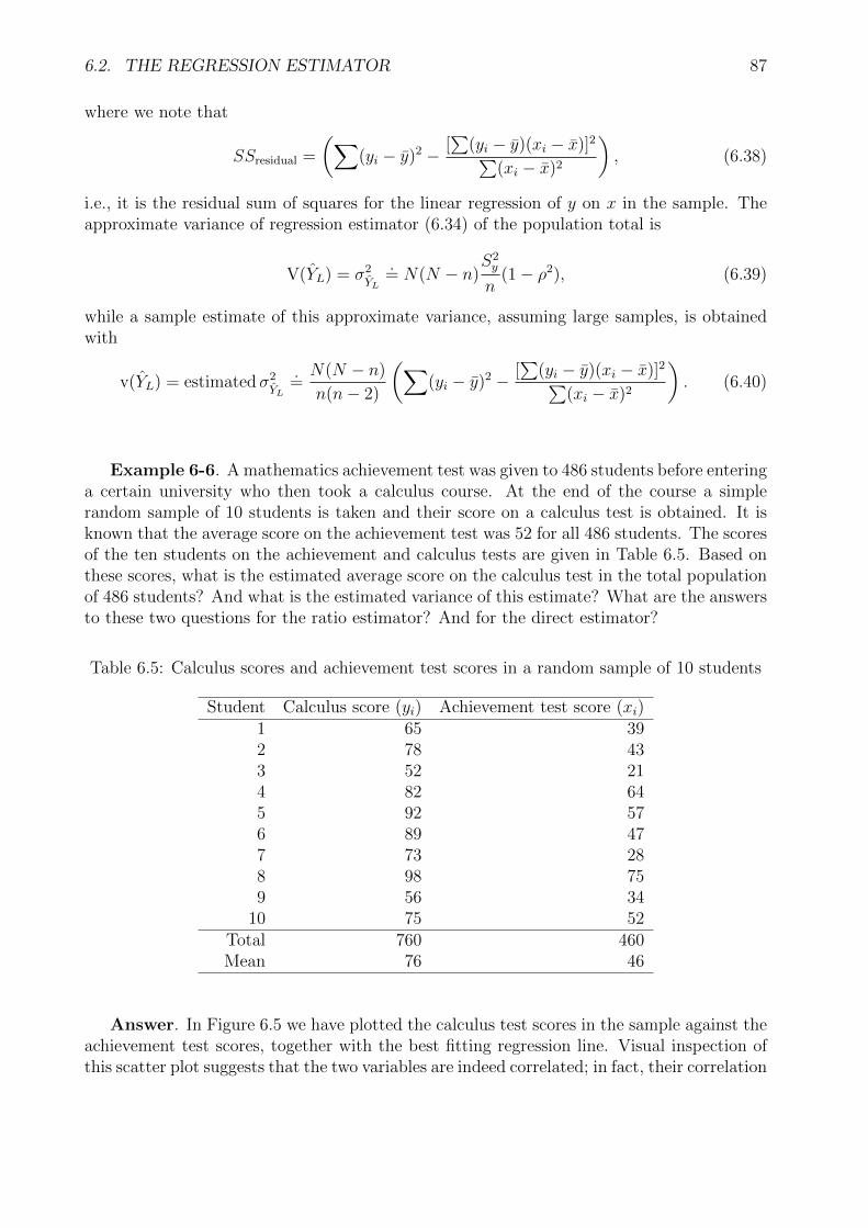
6.2. THE REGRESSION ESTIMATOR 87
where we note that
SSresidual =
(∑(yi − y)2 − [
∑(yi − y)(xi − x)]2∑
(xi − x)2
), (6.38)
i.e., it is the residual sum of squares for the linear regression of y on x in the sample. Theapproximate variance of regression estimator (6.34) of the population total is
V(YL) = σ2YL
.= N(N − n)
S2y
n(1− ρ2), (6.39)
while a sample estimate of this approximate variance, assuming large samples, is obtainedwith
v(YL) = estimated σ2YL
.=N(N − n)
n(n− 2)
(∑(yi − y)2 − [
∑(yi − y)(xi − x)]2∑
(xi − x)2
). (6.40)
Example 6-6. A mathematics achievement test was given to 486 students before enteringa certain university who then took a calculus course. At the end of the course a simplerandom sample of 10 students is taken and their score on a calculus test is obtained. It isknown that the average score on the achievement test was 52 for all 486 students. The scoresof the ten students on the achievement and calculus tests are given in Table 6.5. Based onthese scores, what is the estimated average score on the calculus test in the total populationof 486 students? And what is the estimated variance of this estimate? What are the answersto these two questions for the ratio estimator? And for the direct estimator?
Table 6.5: Calculus scores and achievement test scores in a random sample of 10 students
Student Calculus score (yi) Achievement test score (xi)1 65 392 78 433 52 214 82 645 92 576 89 477 73 288 98 759 56 34
10 75 52Total 760 460Mean 76 46
Answer. In Figure 6.5 we have plotted the calculus test scores in the sample against theachievement test scores, together with the best fitting regression line. Visual inspection ofthis scatter plot suggests that the two variables are indeed correlated; in fact, their correlation

88 CHAPTER 6. ALTERNATIVE METHODS OF ESTIMATION
achievement test score
806040200
calc
ulu
s s
co
re
100
80
60
40
20
0
R2 Linear = 0.705
Figure 6.5: Scatter plot of calculus score against achievement test score, including regressionline
Coefficientsa
Model
Unstandardized Coefficients
t Sig.B Std. Error Beta
1 (Constant)
achievement test score
40.784 8.507 4.794 .001
.766 .175 .840 4.375 .002
a.
Page 1
Figure 6.6: Results of linear regression of calculus score on achievement test score: parameterestimates
is 0.982. It is also clear from this figure, however, that the regression line does not go throughthe origin, meaning that the regression estimator should be used.
The regression equation of the best fitting line on the scores of the 10 students on thesetwo variables is Y = 40.784 + 0.765562X, see Figure 6.6. The t-test for the regressioncoefficient B is very significant (p < 0.01), meaning that there is indeed a strong linearrelationship between the two variables. The t-test for the (Constant) in Figure 6.6 indicatesthat the intercept also very significantly deviates from zero (p < 0.01), confirming that theregression estimator of the average should be used in this case.
Since the sample means are y = 76 and x = 46, see Table 6.5, the regression estimatefollows from (6.33) yielding
yL = y + b(X − x) = 76 + (0.765562)(52− 46) = 80.5934.

6.2. THE REGRESSION ESTIMATOR 89
ANOVAa
Model df Mean Square F Sig.
1 Regression
Residual
Total
1449.974 1 1449.974 19.141 .002b
606.026 8 75.753
2056.000 9
a.
b.
Page 1
Figure 6.7: Results of linear regression of calculus score on achievement test score: ANOVAtable
The sample estimate of the variance follows from (6.37):
v( ˆYL).=
1− 10486
10(10− 2)
(∑(yi − y)2 − [
∑(yi − y)(xi − x)]2∑
(xi − x)2
)= (0.01224279835)
(2056− 18942
2474
)= (0.01224279835)(606.025869) = 7.42.
Using the ratio estimator (6.2) we obtain
ˆYR = yX
x= (76)(
52
46) = 85.91,
while the estimated variance of ˆYR equals
v( ˆYR) =1− n
N
n
[∑ni=1(yi − Rxi)2
n− 1
]=
(1− 10
486
10
)(283.421)
= (0.09794238683)(283.421) = 27.76,
according to (6.19).The (unbiased) direct estimator of the population mean is given by
ˆY =1
n
n∑i=1
yi = y = 76,
see Chapter 2; according to (2.28) its variance is
v(y) =1− n
N
ns2 =
(1− 10
486
10
)(228.44) = (0.09794238683)(228.44) = 22.37.
So we not only see that the regression estimator is the most precise, but also that the ratioestimator is even less precise than the direct estimator in this case.
6.2.2 The regression estimator in stratified random sampling
As with the ratio estimator, Cochran (1977, p.200 cf) also discusses two ways in which aregression estimate of the population total Y can be made in stratified random sampling.

90 CHAPTER 6. ALTERNATIVE METHODS OF ESTIMATION
The first way is again to make a separate regression estimate of the total of each stratumand then add the totals. The second way is to use a combined regression estimate.
For the separate regression estimator of the total we have the formulas
YLs =L∑h=1
Nh[yh + bh(Xh − xh)], (6.41)
the subscript Ls standing for the separate linear regression estimator, while its variance isestimated from the sample with
v(YLs) = estimated σ2YLs
=L∑h=1
N2h(1− nh
Nh)
nh(s2yh − 2bhsyxh + b2
hs2xh). (6.42)
In these formulas, yh and xh are the sample means in stratum h, and Xh is the populationmean of the auxiliary variable X in stratum h. Moreover, syh and sxh are the sample standarddeviations in stratum h, syxh is the sample covariance between y and x in stratum h (see(6.23) for the formula), and
bh =syxhs2xh
, (6.43)
i.e., the sample regression coefficient in the linear regression of y on x in stratum h.This estimator is to be recommended when the regression coefficients βh in the population
are very different, and the sample sizes nh are not too small. When the nh are small there isthe danger of bias, and it is better to use the combined linear regression estimator. In thiscase, the same regression coefficient bc is used in each stratum:
YLs =L∑h=1
Nh[yh + bc(Xh − xh)], (6.44)
with variance
v(YLc) = estimated σ2YLc
=L∑h=1
N2h(1− nh
Nh)
nh(s2yh − 2bcsyxh + b2
cs2xh). (6.45)
The optimal value of bc is the following weighted mean of the bh:
bc =L∑h=1
N2h(1− nh
Nh)s2xh/nh∑L
h=1N2h(1− nh
Nh)s2xh/nh
bh, (6.46)
which – upon substitution of (6.43) – can be written as
bc =L∑h=1
N2h(1− nh
Nh)syxh/nh∑L
h=1 N2h(1− nh
Nh)s2xh/nh
, (6.47)
see Cochran (1977, Section 7.10).

6.2. THE REGRESSION ESTIMATOR 91
6.2.3 Estimation of sample size for the regression estimator
To find the sample size needed to estimate µ = Y when the regression estimator is used, letd = |µ− y| be the margin of error we are willing to tolerate, let t be the value of the normaldeviate corresponding to the desired confidence probability. Then the minimum sample sizerequired follows from
d = tσ ˆYL= t
√(N − nN
)S2y
n(1− ρ2), (6.48)
see (6.36). Solving (6.48) with respect to n we obtain
n =t2S2
y(1− ρ2)
d2 +t2S2
y(1−ρ2)
N
, (6.49)
which reduces to
n0 =t2S2
y(1− ρ2)
d2(6.50)
when N is very large.For the estimation of sample size based on the absolute error d = |Nµ−Ny| of the total
Nµ = Y in the population we have that
d = tσYL , (6.51)
or, upon substitution of (6.39) in (6.51),
d = t
√N(N − n)
S2y
n(1− ρ2). (6.52)
Solving (6.52) for n, we find that
n =t2S2
y(1− ρ2)
d2
N2 +t2S2
y(1−ρ2)
N
, (6.53)
or – if nN< 0.1 –
n0 =t2N2S2
y(1− ρ2)
d2. (6.54)

92 CHAPTER 6. ALTERNATIVE METHODS OF ESTIMATION

Chapter 7
Systematic and repeated sampling
So far we have assumed that we need information on the population at only one point orduring only one period in time. We now consider the situation where we need to observea population two or more times, or during a prolonged period of time. One reason whywe would like to draw two consecutive samples from the population is in order to obtainauxiliary information from the first sample, and then use this information to obtain a moreprecise estimate of the variable of interest in the second sample. This situation is calleddouble sampling and is discussed in Section 7.3. A second reason why we could be interestedin drawing two or more consecutive samples of the population is in order to be able toevaluate changes due to the effect of external forces acting on the population. The questionthen arises: is it best to repeatedly observe the same or different sampling units each time?This is the topic of Section 7.4.
First, however, we discuss yet another sampling method: systematic sampling.
7.1 Systematic sampling
In systematic sampling it is assumed that the N units in the population are numbered 1to N in some order. To select a systematic sample of n units, a unit at random is selectedfrom the first k units and every kth unit thereafter. If k = 15 for example, and if the firstrandomly selected unit is number 13, then the subsequent units are numbers 28, 43, 58, etcetera. The selection of the first unit determines the whole sample. In order for the sampleto “cover” the whole population the value of the integer k should be chosen equal to, orapproximately equal to N
n. This is called an every kth systematic sample.
Consider the artificial population shown in Table 7.1. If a systematic sample of 4 elementsis to be selected from this population, then k is chosen to be k = N
n= 32
4= 8 in order to
cover the whole population. If the first randomly selected number happens to be 5, thenthe sample consists of element numbers 5, 13, 21, and 29, with values 11, 27, 49, and 65,respectively. This is row 5 in Table 7.1.
Since N is not in general an integral multiple of k, different systematic samples from thesame finitie population may vary by one unit in size. With N = 23 and k = 5, for example, atotal of five different systematic samples may be obtained. The three samples starting withunit numbers 1, 2, and 3 have n = 5, while those starting with unit numbers 4 and 5 haven = 4. This introduces a disturbance in the theory of systematic sampling. The disturbanceis negligible if n is larger than 50 and will be ignored here. Even when n is small it is unlikely
93

94 CHAPTER 7. SYSTEMATIC AND REPEATED SAMPLING
Table 7.1: Population of 32 units numbered from 1 to 32
unit value unit value unit value unit valuenumber yi number yi number yi number yi Total Mean
1 1 9 13 17 37 25 53 104 262 3 10 17 18 39 26 61 120 303 3 11 19 19 43 27 63 128 324 5 12 21 20 41 28 57 124 315 11 13 27 21 49 29 65 152 386 11 14 25 22 47 30 65 148 377 11 15 31 23 51 31 71 164 418 15 16 33 24 57 32 75 180 45
to be large. Cochran (1977, p.206) also discusses an alternative systematic sampling methodproviding both a constant sample size and an unbiased sample mean.
A systematic sample can be conceived of as a kind of stratified sample with one observa-tion in each stratum. However, whereas in stratified random sampling random numbers haveto be drawn for each sample unit, in systematic sampling the first random number specifiesfor all strata which fixed unit is selected.
The first advantage of systematic sampling over random sampling is therefore that itonly requires the drawing of one random number instead of n. And we only need to countsimply k units further instead of using a count that changes all the time. If the units in thepopulation are in a certain order, systematic sampling also guarantees that the sample isspread evenly over the population, whereas in random sampling some subpopulations mayaccidentally be underrepresented or even not represented at all.
If N = nk, the mean of a systematic sample, which we will denote by ysy, is an unbiasedestimate of Y for a randomly located systematic sample. Let yij denote the jth element ofthe ith systematic sample, j = 1, . . . , n, i = 1, . . . , k, and let yi denote the mean of the ithsample. Then the variance of the mean of a systematic sample of size n is
V(ysy) = σ2ysy =
N − 1
NS2 − k(n− 1)
NS2wsy, (7.1)
where
S2wsy =
1
k(n− 1)
k∑i=1
n∑j=1
(yij − yi)2 (7.2)
is the variance among units that lie within the same systematic sample, see Cochran (1977,p.208) for a proof.
Example 7-0. Consider the artificial population in Table 7.1. What is the variance ofthe mean for a simple random sample of size n = 4 from this population? And the varianceof the mean for a systematic sample of size n = 4?

7.1. SYSTEMATIC SAMPLING 95
Answer. The variance of the mean for a simple random sample of size n = 4 from thispopulation is obtained from (2.18):
V(y) = σ2y =
S2
n,
with S2 as defined in (2.8). Since the mean of the data in Table 7.1 is Y = 112032
= 35, thevariance of y in the population is
S2 =
∑Ni=1(yi − Y )2
N − 1,=
15, 840
31= 510.9677,
from which it follows that the variance of the mean for a simple random sample of size n = 4is
V(y) =510.9677
4= 127.74.
For the variance of the mean of a systematic sample from the population in Table 7.1 wefirst calculate (7.2):
S2wsy =
1
8(4− 1)(14, 720) = 613.3333,
from which it follows that
V(ysy) =N − 1
NS2 − k(n− 1)
NS2wsy =
32− 1
32(510.9677)− 8(4− 1)
32(613.3333) = 35.
We conclude that – for these data at least – the systematic sample estimate is much moreprecise than the simple random sample estimate.
So how does systematic sampling generally compare with simple and stratified randomsampling? We may distinguish four situations.
1. The manner in which the units of the population are ordered in the sampling frameis completely unrelated to the values of the variable of interest. This is often truewhen units are ordered alphabetically. In this situation a systematical sample will beas precise as a simple random sample, and the variance formulas of Chapter 2 can beused.
2. The numbering of the elements of the population in the sampling frame is based onsome qualitative characteristic, e.g. the location where someone is living. The relativefrequency of these characteristics in a systematic sample will then be very similar totheir frequency in the population. We have basically applied proportional stratification,which is more precise than simple random sampling, see also Chapter 3.
3. The numbers assigned to the units of the population in the sampling frame globallyincrease or decrease with the values of a continuous auxiliary variable (e.g., somemeasure of size) that is highly correlated with the variable of interest. This has theeffect that the means of the research variable are very different in each population layerof k elements. The implicit stratification then obtained with systematic sampling ismuch more precise than simple random sampling, see Example 7-0 where the numberingof the units is clearly correlated with the values of the yi.

96 CHAPTER 7. SYSTEMATIC AND REPEATED SAMPLING
4. When there happens to be a periodic fluctuation in the population – meaning thatpopulation elements with rank numbers in the sampling frame that are a multiple of acertain value c have about the same value – then the variance of a systematic samplewill underestimate the real variance in the population.
In systematic sampling there are some problems to obtain sample estimates of the vari-ance of the mean. According to Moors and Muilwijk (1975) one often approximates thisvariance by using formula (2.28) for simple random sampling without replacement (in sys-tematic sampling an element can never be selected more than once). In the just mentionedsituation 1, no problems arise with this formula, while in situations 2 and 3 the variancewill be estimated as being too large, meaning that we then obtain an estimate of precisionthat can only err on the safe side. Cochran (1977, p.225) provides dedicated formulas forcalculating sample estimates of the variance of the mean in situations 2 and 3, but also warnsthat these variance estimates can be badly biased when applied to the wrong situation.
7.2 Stratified systematic sampling
Just as a simple random sample can be selected from each stratum in stratified randomsampling, we can also draw a systematic sample from each stratum. In the latter case thestarting points of the systematic samples in each stratum should be independently deter-mined. This method will be more precise than stratified random sampling if systematicsampling within strata is more precise than simple random sampling with strata.
If ysyh is the mean of the systematic sample in stratum h, h = 1, . . . , L, the estimate ofthe population mean Y and its variance are
ystsy =L∑h=1
Whysyh, (7.3)
and
V(ystsy) = σ2ystsy =
L∑h=1
W 2hV(ysyh). (7.4)
The problem of finding a sample estimate of this variance is the same as discussed in theprevious section.
7.3 Double sampling
Double sampling is a sampling method where initially a random sample is selected for thepurpose of obtaining auxiliary information only, after which a second random sample isdrawn from the first sample in order to observe the actual variable of interest in addition tothe auxiliary variable. Double sampling, also known as two-phase sampling, is not only usefulfor obtaining auxiliary information for ratio and regression estimation (see Chapter 6), butalso for finding information for stratified random sampling (see Chapter 3) and for handlingnon-response.

7.3. DOUBLE SAMPLING 97
7.3.1 Double sampling for ratio estimation
Let yi be the variable of interest, xi be the auxiliary variable, n′ be the number of units inthe first sample, which includes the second sample, and let n < n′ be the number of units inthe second sample. Variables xi and yi are only observed in the second sample. In the firstsample only xi is observed. It is assumed that the observation of the yi is expensive whereasthe observation of the xi is (much) cheaper.
If the first sample is used to obtain
x′ =1
n′
n′∑i=1
xi, (7.5)
as an estimate of X in a ratio estimate of the population mean Y , the ratio estimator of thepopulation mean Y is
yR = Rx′ =
∑ni=1 yi∑ni=1 xi
x′, (7.6)
with approximate variance equal to
V(yR) = σ2yR
.=
(1
n′− 1
N
)S2y +
(1
n− 1
n′
)(S2
y − 2RSyx +R2S2x). (7.7)
and estimated variance equal to
v(YR) = estimated σ2YR
=(N − n′)
N
s2y
n′+
n′ − nn′n(n− 1)
n∑i=1
(yi − Rxi)2. (7.8)
The ratio estimator of the population total Y is
YR = RX =
∑ni=1 yi∑ni=1 xi
X, (7.9)
and
X =N
n′
n′∑i=1
xi. (7.10)
The estimated variance of this estimator is
v(YR) = estimated σ2YR
= N(N − n′)s2y
n′+N2 n′ − n
n′n(n− 1)
n∑i=1
(yi − Rxi)2. (7.11)
Example 7-1. A forest resource manager is interested in estimating the total number ofdead trees in a 400 acre area of heavy infestation. He divides the area in 200 plots of equalsize and uses arial photo counts to find the number of dead trees in a random sample of 18plots. He then randomly samples 8 plots out of these 18 plots and conducts a ground count

98 CHAPTER 7. SYSTEMATIC AND REPEATED SAMPLING
Table 7.2: Counts of dead trees in a random sample of 8 plots
arial photo count arial photo countPlot first sample (x′i) second sample (xi) ground count (yi)
1 52 7 7 93 10 10 134 65 7 7 106 9 9 117 38 69 8
10 1111 512 9 9 1013 1214 1315 3 3 416 20 20 2517 15 15 1718 4
Total 153 80 99
on these 8 plots. The resulting counts are given in Table 7.2. Based on these counts, whatis the estimated total number of dead trees in the 400 acre area? And what is the estimatedvariance of this estimate?
Answer. In this example N = 200, n′ = 18, and n = 8, and the estimated total numberof dead trees in the 400 acre area is
YR = RX =
∑ni=1 yi∑ni=1 xi
N
n′
n′∑i=1
xi =
(99
80
)(200
18
)(153) = 2, 103.75.
Since s2y =
∑ni=1(yi−y)2
n−1= 39.4384 and
∑ni=1(yi − Rxi)2 = 6.1928, the estimated variance of
this estimate equals
v(YR) =N(N − n′)s2
n′+N2 n′ − n
n′n(n− 1)
n∑i=1
(yi − Rxi)2
=200(200− 18)
(39.4384
18
)+ 2002
(18− 8
(18)(8)(8− 1)
)(6.1928)
=79, 753.20889 + 2, 457.460317 = 82, 210.66921.

7.3. DOUBLE SAMPLING 99
7.3.2 Double sampling for regression estimation
In some applications of double sampling the auxiliary variable xi is used to obtain a regressionestimate of the population mean Y . Just as in double sampling for ratio estimation, in thefirst (large) sample of size n′, only xi is measured. In the second step, a random subsampleof size n = n′
kis taken, and both xi and yi are measured.
Letting yi and xi be known for every unit in the sample, and let the population meanµx = X of the xi also be known. Then the linear regression estimator of Y , the populationmean of the yi, is
yL = y + b(x′ − x), (7.12)
where x′ and x are the means of the xi in the first and second samples, and b is the leastsquares regression coefficient of yi on xi, computed for the second sample. Just as in one-stagesampling, this regression estimator will be biased, see also Section 6.2.
Assuming random sampling and 1n′ and 1
nnegligible withe respect to 1, the approximate
variance of regression estimator (7.12) of the population mean is
V( ˆYL) = σ2ˆYL
.=S2y(1− ρ2)
n+S2yρ
2
n′−S2y
N, (7.13)
where ρ = Syx
SySx, the population correlation between y and x, Sy and Sx are the standard
deviation of y and x in the population, respectively, and Syx is their population covariance.See Cochran (1977, p.339) for a proof.
If terms in 1n
are negligible, a sample estimate of V( ˆYL) is
v( ˆYL) = estimated σ2ˆYL
.=s2y.x
n+s2y − s2
y.x
n′−s2y
N, (7.14)
where
s2y.x =
1
n− 2
(n∑i=1
(yi − y)2 − b2(n∑i=1
(xi − x)2)
)(7.15)
is an unbiased estimate of S2y(1− ρ2) and
s2y =
∑ni=1(yi − y)2
n− 1(7.16)
is an unbiased estimate of S2y .
If the second sample is small and terms in 1n
are not negligible relative to 1, an estimateof variance is
v( ˆYL) = estimated σ2ˆYL
= s2y.x
(1
n+
(x′ − x)2∑ni=1(xi − x)2)
)+s2y − s2
y.x
n′−s2y
N, (7.17)
see also Cochran (1977, p.343).

100 CHAPTER 7. SYSTEMATIC AND REPEATED SAMPLING
7.3.3 Double sampling for stratification
Double sampling can also be used when stratified random sampling is the method of pref-erence, but the sizes of the different strata in the population are unknown. A large simplerandom sample of size n′ is drawn from the total population of N units, and the only ob-servation made in this fist large sample is how many units n′h (h = 1, . . . , L) are in eachstratum. Unbiased estimates of the population stratum sizes Wh = Nh
Nare then obtained
from wh =n′h
n′ . Next, a second sample is selected by stratified random sampling from thefirst sample. These units are classified into strata with nh units selected from the n′h sampleunits in stratum h, and the variable of interest yhi is obtained for each unit in this secondsample. Letting yh =
∑nh
i=1yhinh
denote the sample mean of stratum h in the second sample,
an unbiased estimate of the population mean Y =∑WhYh is obtained with
yst =L∑h=1
whyh. (7.18)
The objective of the first sample is therefore to estimate the strata weights Wh; that of thesecond sample is to estimate the strata means Yh. The variance of yst is
V(yst) = σ2yst = S2
(1
n′− 1
N
)+
L∑h=1
WhS2h
n′
(n′hnh− 1
), (7.19)
where S2 is the population variance. An unbiased sample estimate for this variance is
v(yst) = estimated σ2yst =
(N − n′
N
)(1
n′ − 1
) L∑h=1
wh(yh − yst)2
+N − 1
N
L∑h=1
(n′h − 1
n′ − 1− nh − 1
N − 1
)whs
2h
nh, (7.20)
where s2h is the stratum sample variance in the second sample.
Example 7-2. A shoe store wants to estimate the average number of pairs of shoesowned by the students living in a certain college town neighbourhood. They reason that astratified sample based on gender could be a good approach but do not know the distributionof the gender in that neighbourhood. They also do not know the gender of the respondentuntil after contacting them. They therefore use double sampling by first contacting 160randomly selected students in that neighbourhood and ask them about their gender. Theyfind that this first sample consists of 64 males and 96 females. They next randomly sample8 males and 12 females from the 64 males and 96 females in this first sample, and ask themto count the number of pairs of shoes that they have at home and report back to them. Thedata for this second sample are given in Table 7.3. Based on these observations, what is theestimated average number of pairs of shoes these students own? And what is the estimatedvariance of this average?
Answer. In this example the size of the first sample is n′ = 160, with n′1 = 64 malesand n′2 = 96 females. The unknown proportion W1 = N1
Nof males in the population is

7.3. DOUBLE SAMPLING 101
Table 7.3: Number of pairs of shoes owned by 8 male and 12 female students
Male Female5 176 199 135 169 87 115 158 19
12133320
Total 54 196
therefore estimated to be w1 =n′
1
n′ = 64160
= 0.4, and the unknown proportion W2 = N2
Nof
females in the population is estimated to be w2 =n′
2
n′ = 96160
= 0.6. In the second sample,the average number of pairs of shoes for males is found to be y1 = 54
8= 6.75 with a variance
of s21 = 3.073, and that for females is found to be y2 = 196
12= 16.33 with a variance of
s22 = 40.5769, see Table 7.3. The estimated average number of pairs of shoes owned by the
total student population in that neighbourhood is therefore estimated to be
yst =L∑h=1
whyh = (0.4)(6.75) + (0.6)(16.33) = 12.498.
We do not know N , the total number of students in that neighbourhood. However, if weassume it to be quite large, (7.20) can be simplified to
v(yst) =
(1
n′ − 1
) L∑h=1
wh(yh − yst)2 +L∑h=1
(n′h − 1
n′ − 1
)whs
2h
nh,
yielding
v(yst) =
(1
160− 1
)(0.4(6.75− 12.498)2 + 0.6(16.33− 12.498)2
)+
(64− 1
160− 1
)(0.4)(3.073)
8+
(96− 1
160− 1
)(0.6)(40.5769)
12= 0.13853 + 1.2731 = 1.4116.
7.3.4 Double sampling for non-response
An ingenious application of double sampling is the adjustment for non-response in a survey.In this case the first sample of size n′ is a simple random sample from a population of N

102 CHAPTER 7. SYSTEMATIC AND REPEATED SAMPLING
units. These units are then stratified in two strata: n′1 contains those sample units thatrespond, and n′2 = n′ − n′1 consists of the sample units that do not respond. In the second
phase another random sample of size n2 =n′
2
k< n′2 is drawn from the n′2 non-respondents in
the first round and a massive effort is made to obtain information on the variable of interestfor all these n2 units. We have then a double sampling setting where n′1 = n1, and n2 is thesize of the second sample.
Example 7-3. In a university of 1000 students, a questionnaire is mailed to a simplerandom sample of 106 students asking them about the amount of time they spend studyingeach week. Out of these 106 students 46 respond. From the 60 non-respondents, a simplerandom sample of 20 is selected and intensive efforts are made by telephone and personal visitto obtain responses. This yields the data shown in Table 7.4. Based on these observations,what is the estimated average number of hours these students study each week? And whatis the estimated variance of this average?
Table 7.4: Double sampling for average number of hours spent studying per week
Students responding Students contactedto questionnaire and responding to telephone
(first round) and visit (second round)Sample mean 20.5 10.9
Sample standard deviation 6.2 5.1Sample size 46 20
Answer. In this example the first sample of n′ = 106 students can be stratified into thefollowing two strata: the respondents with a size of n′1 = 46 and the non-respondents witha size of n′2 = 60. The unknown proportion W1 = N1
Nof respondents in the population is
therefore estimated to be w1 =n′
1
n′ = 46106
= 0.434, and the unknown proportion W2 = N2
N
of non-respondents in the population is estimated to be w2 =n′
2
n′ = 60106
= 0.566. In thenext step a second random sample of n2 = 20 is drawn from the n′2 = 60 students in thenon-respondent stratum of the first sample. The average of the first stratum in the firstsample is y1 = 20.5 hours with a standard deviation of s1 = 6.2; the average of the secondstratum in the second sample is y2 = 10.9 hours with a standard deviation of s2 = 5.1, seeTable 7.4. The estimated average number of hours spent studying in the total population ofN = 1000 students is therefore estimated to be
yst =L∑h=1
whyh = (0.434)(20.5) + (0.566)(10.9) = 15.0664.
According to (7.20), and because n′1 = n1 = 46 in this case, the estimated variance of this
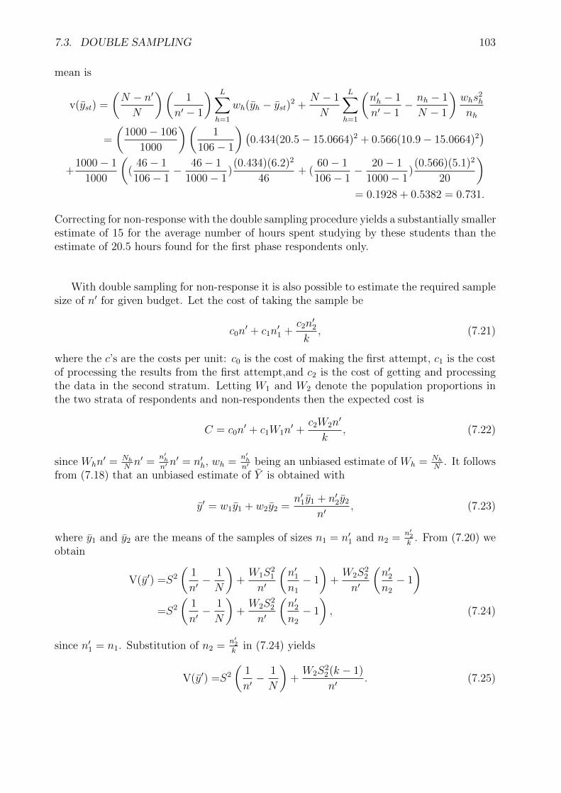
7.3. DOUBLE SAMPLING 103
mean is
v(yst) =
(N − n′
N
)(1
n′ − 1
) L∑h=1
wh(yh − yst)2 +N − 1
N
L∑h=1
(n′h − 1
n′ − 1− nh − 1
N − 1
)whs
2h
nh
=
(1000− 106
1000
)(1
106− 1
)(0.434(20.5− 15.0664)2 + 0.566(10.9− 15.0664)2
)+
1000− 1
1000
((
46− 1
106− 1− 46− 1
1000− 1)(0.434)(6.2)2
46+ (
60− 1
106− 1− 20− 1
1000− 1)(0.566)(5.1)2
20
)= 0.1928 + 0.5382 = 0.731.
Correcting for non-response with the double sampling procedure yields a substantially smallerestimate of 15 for the average number of hours spent studying by these students than theestimate of 20.5 hours found for the first phase respondents only.
With double sampling for non-response it is also possible to estimate the required samplesize of n′ for given budget. Let the cost of taking the sample be
c0n′ + c1n
′1 +
c2n′2
k, (7.21)
where the c’s are the costs per unit: c0 is the cost of making the first attempt, c1 is the costof processing the results from the first attempt,and c2 is the cost of getting and processingthe data in the second stratum. Letting W1 and W2 denote the population proportions inthe two strata of respondents and non-respondents then the expected cost is
C = c0n′ + c1W1n
′ +c2W2n
′
k, (7.22)
since Whn′ = Nh
Nn′ =
n′h
n′ n′ = n′h, wh =
n′h
n′ being an unbiased estimate of Wh = Nh
N. It follows
from (7.18) that an unbiased estimate of Y is obtained with
y′ = w1y1 + w2y2 =n′1y1 + n′2y2
n′, (7.23)
where y1 and y2 are the means of the samples of sizes n1 = n′1 and n2 =n′
2
k. From (7.20) we
obtain
V(y′) =S2
(1
n′− 1
N
)+W1S
21
n′
(n′1n1
− 1
)+W2S
22
n′
(n′2n2
− 1
)=S2
(1
n′− 1
N
)+W2S
22
n′
(n′2n2
− 1
), (7.24)
since n′1 = n1. Substitution of n2 =n′
2
kin (7.24) yields
V(y′) =S2
(1
n′− 1
N
)+W2S
22(k − 1)
n′. (7.25)

104 CHAPTER 7. SYSTEMATIC AND REPEATED SAMPLING
The quantities n′ and k are then chosen to minimize the product C(V + S2
N). From (7.25)
and (7.22) we have
V +S2
N=
(S2 −W2S22)
n′+kW2S
22
n′. (7.26)
and
C = (c0 + c1W1)n′ +c2W2n
′
k. (7.27)
Optimizing C(V + S2
N) with respect to k, it is not very difficult to verify that the optimum
is found for
kopt =
√c2(S2 −W2S2
2)
S22(c0 + c1W1)
. (7.28)
The initial sample size n′ can be chosen either to minimize C for given V , or V for givenC by solving n′ from (7.26) or (7.27). If V is specified, it follows from (7.26) that
n′opt =N(S2 + (k − 1)W2S
22)
NV + S2, (7.29)
where V is the variance (7.25) of the estimated population mean. For given total budget C,on the other hand, it follows from (7.27) that
n′opt =kC
k(c0 + C1W1) + c2W2
. (7.30)
The solution requires a knowledge of W2. This can often be estimated from previousexperience. Moreover, in addition to S2, the variance in the population whose value mustbe estimated in advance in any problem of sample size, we also need an estimate of S2
2 , thevariance in the non-response stratum. The latter value may be harder to predict, and itwill probably not be the same as S2. In surveys made by mail of economic enterprise, forexample, the respondents tend to be larger operators, with larger between-unit variancesthan the non-respondents.
If W2 is not well-known, Cochran (1977) suggests to obtain an approximation of n′optfrom (7.28) and (7.29) by substituting a range of assumed values of W2 between 0 and asafe upper limit, and then to use the maximum n′opt in this series as the initial sample sizen′. When the replies to the mail survey have been received, the value of n′2 is known. Inorder to obtain a value for k with this method, the variance Vc(y
′) conditional on the knownvalues of n2 and n′ should be used. This variance is
Vc(y′) =S2
(1
n′− 1
N
)+n′2S
22(k − 1)
n′2. (7.31)
Equation (7.31) is solved to find the k that gives the desired conditional variance. The costfor this method is usually only slightly higher than the optimum cost for known W2.
With stratified sampling, the optimum values of the n′h and the kh in the individual strataare rather complex. According to Cochran (1977), a good approximation is to estimate first,

7.3. DOUBLE SAMPLING 105
by the methods in Section 3.4 and Section 3.6, the sample sizes nh that would be requiredin the strata if there were no non-response. Then, from (7.29), if W2 = 0, we have
n′0 =NS2
NV + S2, (7.32)
and (7.29) can therefore be written as
n′opt = n0
(1 +
(k − 1)W2S22
S2
). (7.33)
Applying the latter equation separately to each stratum gives an approximation to theoptimal n′h. The values of kh are found by applying (7.28) in each stratum.
These techniques can also be used with the ratio or the regression estimator. With theratio estimator, the quantities S2 and S2
2 are replaced by S2d and S2
2d, where di = yi − Rxi.With the regression estimator, S2 becomes S2(1− ρ2) and S2
2 becomes S22(1− ρ2).
Example 7-4. In a university of 1, 000 students, we want to find the average amountof money the students spend on living. We expect the non-response to be about 40%. It isalso expected that the respondents have a larger variance than the non-respondents. Theoverall variance in the population is estimated to be S2 = 120 while the variance for thenon-respondents is estimated to be S2
2 = 80. The initial costs of sampling each respondent is0, the cost of a standard response is 1, and the cost of a call-back is 4. What is the numberof students to sample in the first round, and how many students should be subjected to acall-back, if we require the variance of the estimator to be equal to 5?
Answer. We have c0 = 0, c1 = 1 and c2 = 4. Moreover, W1 = 0.6 and W2 = 0.4. Theoptimal value for k, the fraction to sample from the non-respondents in the first sample, canbe found with (7.28):
kopt =
√c2(S2 − w2S2
2)
S22(c0 + c1w1)
=
√(4)(120− (0.4)(80))
(80)(1)(0.6)=
√352
48= 2.71.
Since V = 5 the optimal size of the first sample is obtained using (7.29):
n′opt =N(S2 + (k − 1)w2S
22)
NV + S2=
1000(120 + (2.71− 1)(0.4)(80))
(1000)(5) + 120=
174, 720
5, 120= 34.125.
Rounding up we have n′ = 35, from which it follows that n′2 = w2n′ = (0.4)(35) = 14. So
for a precision of V = 5 we require a random sample of 35 students in the first phase, and
we need to call back n2 =n′
2
k= 14
2.71= 5.16, i.e., 6 students in the second phase.
Example 7-5. In a survey the first sample is taken by mail and the response is expectedto be about 50%. The precision desired is that which would be given by a simple randomsample of size 1, 000 if there were no non-response. The cost of mailing a questionnaire is10 cents, and the cost of processing the completed questionnaire is 40 cents. To carry out a

106 CHAPTER 7. SYSTEMATIC AND REPEATED SAMPLING
personal interview costs 4.10 euro’s. How many questionnaires should be sent out and whatpercentage of the non-respondents should be interviewed?
Answer. We have c0 = 0.10, c1 = 0.40, and c2 = 4.50. The precision desired is V = S2
1000.
Moreover, W1 = W2 = 0.5. If the variances S2 and S22 are assumed to be equal, and N is
assumed to be large it follows from (7.28) that
kopt =
√c2(S2 −W2S2
2)
S22(c0 + c1W1)
=
√c2(1−W2)
c0 + c1W1
=
√(4.5)(0.5)
0.10 + (0.40)(0.5)= 2.739,
and from (7.29) that
n′opt =N(S2 + (k − 1)W2S
22)
NV + S2=
(S2 + (k − 1)W2S22)
V + S2
N
.=
(S2 + (k − 1)W2S22)
V
=(S2 + (k − 1)W2S
22)
S2
1,000
= 1, 000(1 + (k − 1)W2) = 1, 000(1 + (2.739− 1)(0.5)) = 1, 869.5.
This means that 1, 870 questionnaires should be mailed, and of the 935 expected not to bereturned a random sample of 935
2.739= 341 should be interviewed. The total cost of the survey is
C = (c0+c1W1)n′+ c2W2n′
k= (0.10+(0.40)(0.5))(1, 870)+ (4.50)(0.5)(1,870)
2.739= 561+1, 536 = 2, 097
euro’s.
7.4 Continuous sampling
So far we have assumed that we need information on the population at only one point orduring only one period in time. We now consider the situation where we need to investigatea population several times or during a prolonged period of time. The question then arises:is it best to repeatedly observe the same or different sampling units each time?
As discussed by Cochran (1977, Section 12.10), given the data from a consecutive seriesof samples, the answer to this question depends on the kind of quantity for which we maywish estimates:
• The change in Y from one occasion to the next?
• The average value of Y over all occasions?
• The average value of Y for the most recent occasion?
We first consider the case of two consecutive surveys. Let the population variables ofinterest on the two occasions be x and y, respectively, and their correlation be ρ. Furtherassume that both samples are random and of equal size, and that the finite populationcorrection is negligible. Suppose that the randomly selected part W of the first sample isreplaced by other randomly selected elements on the second occasion, while the other part1−W (the permanent part) remains the same. We distinguish three situations:
• The purpose of the data collection is the estimation of changes over time in the meansX and Y , or totals X and Y . This is most appropriate if we want to study the effectsof forces that are known to have affected the population of interest. In this case we

7.4. CONTINUOUS SAMPLING 107
want the estimated difference ˆX − ˆY to be as accurate as possible. Both the mean ofthe permanent part x′ and the mean x′′ of the rest is then an unbiased estimator ofX. An unbiased estimator of X is obtained with the following weighted average:
ˆX = Wx′ + (1−W )x′′ (7.34)
for the first survey, and
ˆY = Wy′ + (1−W )y′′ (7.35)
for the second survey, where x′ and y′ are obtained from the same sample fraction, andx′′ and y′′ from two different sample fractions. Because the different sample fractionsare independent we have that
V( ˆY − ˆX) = W 2V(y′ − x′) + (1−W )2V(y′′ − x′′). (7.36)
For the two variances on the right side of (7.36) we find that
V(y′ − x′) =1
Wn(S2
x − 2ρSxSy + S2y), . (7.37)
the sample size of this part being Wn, and
V(y′′ − x′′) = V(y′′) + V(x′′) =1
(1−W )n(S2
x + S2y), (7.38)
y′′ and x′′ being calculated from two independent samples of size (1−W )n. Substitutionof (7.37) and (7.38) in (7.36) yields
V( ˆY − ˆX) =1
n(S2
x − 2WρSxSy + S2y). (7.39)
When ρ is positive, which is the usual situation, it follows from (7.39) that the precision
of the difference ˆX − ˆY is maximised by choosing W as large as possible. Since thislargest value is W = 1, we see that precision in measuring change is largest when therandom sample on the two occasions is left unchanged. In practice this is not alwaysfeasible, because part of the population ceases to exist (e.g., emigration) while anotherpart of the population is renewed (e.g., immigration).
• The purpose of the data collection is to estimate the sum or average on the twooccasions as accurately as possible. Again starting from (7.34) we now find that
V( ˆY + ˆX) =1
n(S2
x + 2WρSxSy + S2y). (7.40)
Again assuming ρ to be positive, it follows from (7.40) that the precision of the sumˆX + ˆY is maximised by choosing W as small as possible. Since this smallest value isW = 0, we see that precision in measuring the average or total of the two occasionsis largest when the random sample of the first occasion is completely replaced on thesecond occasion.

108 CHAPTER 7. SYSTEMATIC AND REPEATED SAMPLING
• The purpose of the data collection is to estimate the value of Y or ˆY as accurately aspossible on the second occasion. In this case we can replace part, usually at least onehalf, of the sample and apply two-phase or double sampling (see Section 7.3) with aregression estimator.
When the population is observed on more than two occasions, for the already mentionedpractical reasons one often uses gradual rotation of the sample. In the second year, forexample, one quarter of the previous sample is replaced, in the third year yet another quarterof the original sample is replaced, et cetera, meaning that the whole sample will have beenrotated after the fourth year. In this way, no one will be part of the sample for more thanfour years. On this topic Cochran (1977, Chapter 12) further concludes that “field costs arelikely to be lower if the same units are retained for a number of occasions. If estimates ofthe change in the population total or mean are of interest, this factor also points towardmatching more than half the units from one occasion to the next. It is convenient to keepthe weights and the proportion matched constant, instead of changing them every occasion.... increase in the proportion matched from 1
2to 3
4produces substantial gains in efficiency for
the estimates of change at the expense of smaller losses in efficiency for the current estimates.The results suggest that retention of 1
2, 3
4, or 4
5from one occasion to the next may be a good
practical policy if current estimates and estimates of change are both important.”

Chapter 8
Other sources of error
In the previous chapters we only discussed sampling error as a potential source of deviationbetween population values and their sample estimates. Sampling errors arise due to thefact that we only investigate part of the population, and they disappear when the wholepopulation is observed. In this chapter we discuss other sources of error not considered sofar.
8.1 Problems with the sampling frame
In this section we follow the recommendations on (the solution of) problems with the sam-pling frame as discussed in Moors and Muilwijk (1975). The sampling frame is the admin-istrative counterpart of the population of interest. It usually consists of one or more lists ordatabases containing all elements of the population, but this is not necessary as long as asystematic description is provided of the way in which the elements can be found. Militarymaps, for example, can be used as a frame for all parcels in a region, and these need not beput on a list. In the case of two-stage sampling (see Chapter 5), a frame for all secondaryunits is not required: it is enough to have a frame of all primary units together with framesof the elements within each of the randomly drawn primary units.
There are three problems that can arise with sampling frames: missing elements, elementsthat are included more than once, and elements that do not belong to the population ofinterest. In these cases three general approaches may be considered:
• We can try and correct the complete sampling frame. This approach, however, is bothcostly and time-consuming.
• We can redefine the population according to the possibilities offered by the frame.
• We can ignore the problems and consider the frame to be ideal. If the effect on theresults is small, this approach can hardly be argued against.
Several of these problems arise because the frame always slightly lags behind the actualsituation. Even when changes in the population are reported quickly, delays occur in theadministrative processing of the mutations.
109

110 CHAPTER 8. OTHER SOURCES OF ERROR
8.2 Missing elements
Incompleteness of the frame is a frequent problem, that is also often difficult to fix. We canhave random missing elements, as a result of errors or mistakes, and a systematical lack ofinformation for certain subpopulations. An example of the latter situations concerns newelements of the population that have not yet been processed. There are two conceivablemethods to solve for incompleteness of the frame. The first method is to use two differentframes of the same population, if available. By comparing the two frames, random missingelements may be tracked down, and often also systematic missing elements. With this firstmethod we may again distinguish two cases:
• We use frame 1, with the missing elements in 1 supplemented from frame 2. This isonly feasible when frame 2 is not too large.
• Frames 1 and 2 are used together. This, however, results in new problems becausesome elements will be registered in both frames, see also Section 8.4.
In the nineteen seventies in the Netherlands passenger cars were in principle registered twice,for example: once in the database of the “Dienst motorrijtuigenbelasting” (Center of motorvehicle taxes) and once in the license plate database of the Dutch “Rijksdienst Wegverkeer”(Vehicle Technology and Information Center). The first database was easy to use becauseit had been computerized, but it was also incomplete; at that time the second database wastherefore used to supplement the first.
As a second example, the population registers of all Dutch municipalities together are asampling frame for the Dutch population, except for the sailing and traveling population.Until the ninety nineties these people without fixed address were registered in the “Centraalpersoonsregister” (Central population register), and the missing elements in the former framecould therefore be supplemented with the elements in the latter frame.
The second method to control for missing elements is during the survey; this is mainlyuseful for tracking down small numbers of missing elements. With this method, it is checkedfor each unit in the sample whether the next unit of the population is registered in thesampling frame. If it is not, the latter unit is added to the sample and also measured (andthe next if it is also missing from the frame).
8.3 Foreign elements
It often happens that the sampling frame contains elements that do not belong to the popula-tion of interest. These are called foreign elements. If it is not possible to remove them beforesampling, they have to be eliminated before observation or at least before computation ofthe population estimates.
One way to handle the problem of foreign elements that was already mentioned in Sec-tion 2.10 is to consider the sampling frame to be a hyperpopulation consisting of the samplingpopulation plus the foreign elements. The sampling population is then a subpopulation inthe sense discussed in Section 2.10. For simple random sampling the formulas in the lattersection can then be applied, and for stratified random sampling those in Section 3.11. How-ever, there we already noticed that when the size of a subpopulation is unknown the precisionof sample estimates is strongly reduced, unless the subpopulation is almost as large as the

8.3. FOREIGN ELEMENTS 111
total population. This procedure also has the effect that the size of the sample from theframe will be smaller (because it will contain foreign elements which have to be removed),but this can be compensated by estimating the reduction in size as well as possible and thenincrease the original sample size accordingly.
Example 8-1. From a neigbourhood of 400 houses we want to draw a simple randomsample of 100 houses from the municipal address register. The latter register, however, alsocontains the addresses of 100 buildings not destined and used for housing. This register isconsidered to be a hyperpopulation consisting of the sampling population (the 400 houses)and the foreign elements (the 100 buildings). The desired sampling fraction of 1
4is applied to
the complete frame. This yields a random sample of n = 125, of which approximately 25 willbe buildings; these are removed from the sample, and the formulas discussed in Section 2.10are used.
Another way to handle the problem of foreign elements is to replace each foreign elementencountered in the sample with the next element in the frame that does belong to the pop-ulation of interest. This means that the sampling probabilities for the population elementsare no longer equal, and usually will have to be evaluated during the field work. This is doneby establishing for each element in the sample how many foreign elements were preceding itin the frame. The sampling probability for each element is then proportional to this countplus one.
Example 8-2. For the same situation as in Example 8-1, a sampling fraction of 100500
= 15
is applied to the complete frame, and elements are drawn randomly without replacement.This yields a random sample of size 100. Now suppose that the first part of the samplingframe has the structure shown in Table 8.1, where h is a house, f is a foreign element, andyi is some characteristic of house or building i (e.g., its financial value).
Table 8.1: A sampling frame with foreign elements
h h h f h f f h h h f h h h h . . . hy1 y2 y3 y4 y5 y6 y7 y8 y9 y10 y11 y12 y13 y14 y15 . . . y500
Also suppose that the first six elements in the random sample of size 100 happen to bethe numbers 2, 12, 9, 3, 7, and 5. Then the first element in the sample, element 2, is ahouse, see Table 8.1, so it stays in the sample; its probability of being selected is p2 = 1
500,
since it is not preceded by a foreign element in the frame. The second element in the sampleis element 12, which is also a house. It therefore stays in the sample. It is preceded by aforeign element in the frame, and its probability of being selected is therefore p12 = 2
500. The
third element in the sample is 9, which is a house not preceded by a foreign element in theframe, so it stays in the sample and has a probability of being selected equal to p9 = 1
500.
The fourth element in the sample is element 3, which is also a house not preceded by a

112 CHAPTER 8. OTHER SOURCES OF ERROR
foreign element in the frame, so it stays in the sample and also has a probability of p3 = 1500
of being selected. The fifth element in the sample is element 7. It is not a house, so it isremoved from the sample and replaced by element 8 in the frame. The latter element hastwo foreign elements preceding it in the frame, so it has a probability of p8 = 3
500of being
selected. The sixth element in the sample is element 5. This is a house so it stays in thesample; it is preceded in the frame by a foreign element, so its probability of being selectedis p5 = 2
500. An unbiased estimate of the population total is therefore
Y =1
n
n∑i=1
yipi
= (y2 +y12
2+ y9 + y3 +
y8
3+y5
2+ . . . ),
see also Chapter 4.
8.4 Multiple registration of elements
When the sampling frame contains some elements more than once, the sampling probabilitiesfor those elements are proportional to the number of times they are registered. We maydistinguish between these three cases:
• The number of registrations per element is known or can be easily established. In thissituation the formulas of Chapter 4 can be applied. The first method is particularlysimple when the multiple registrations of one element are recorded together. As theframe of all practitioners of anthropology, for example, the member lists of all soci-eties of anthropology can be used. By incorporating a question in the survey aboutthe number of these societies of which an anthropologist is a member, the samplingprobability of each member of the sample can be established.
• If one of the multiple registrations can always be distinguished from the others thenthe latter registrations can be considered foreign elements, to be treated using theprocedures discussed in Section 8.3. When the multiple registrations are registeredone after the other in the frame, for example, we may decide that the element is onlyadded to the sample if the first registration of these registrations is selected.
• A large part of the frame consists of single registrations; multiple registrations onlyoccur in another part of the frame. This situation arises when multiple frames areused, for example. The frame with multiple registrations can then be considered asa stratum containing foreign elements. As already discussed in Section 8.2, in thenineteen seventies passenger cars were in principle registered twice in the Netherlands:once in the database of the Center of motor vehicle taxes and once in the license platedatabase of the Dutch Vehicle Technology and Information Center. The latter databasecould be used to supplement the former. For each sampled element from the licenseplate database it is checked whether it is also registered in the vehicle taxes database;if so, it is put aside as a foreign element. For the stratum of the license plate databasethe formulas of Section 2.10 now apply.

8.5. NON-RESPONSE 113
8.5 Non-response
In almost every survey it is found to be impossible to obtain all the required informationfrom each element sampled from the population. Reasons can be absence, illness or theunwillingness of the people in the sample to participate. There are several ways to minimizeor handle this phenomenon which is known as non-response. Non-response introduces biasin the parameter estimates because non-respondents are usually different on the variable(s)of interest from those of the population who do participate.
A good preparation of the survey often makes it possible to restrict the amount of non-response as much as possible. The influence of absence of respondents can be reduced bychoosing a suitable time for interviewing, e.g., not during holidays. The interviewing ofheads of households should preferably be organized in the evenings, after an appointmenthas been made by mail or telephone.
Interviews should be designed such that refusal of cooperation is prevented as much aspossible. In the introduction to the survey the interest of the interviewee should be aroused,the purpose of the interview must clearly be explained, a questionnaire sent by mail shouldcome with an introduction letter, an interviewer should identify himself. The questionsshould be short and clear. As many guarantees of protection of privacy as possible shouldbe provided.
Even though the reduction of non-response can often be successful, one has to take intoaccount that there will always be some sample elements for which no data can be obtained. Itis therefore usually necessary to assess the adverse effects of non-response as best as possible,or to correct for its effects.
When the cause of the non-response is unknown or if there is reason to believe thatits cause is temporary, the first obvious approach to handle non-response is to repeat theattempt to obtain the required information or to make the respondent cooperate in thesurvey.
A second option is to draw a random sample from the non-respondents in the originalsample, and then to try again to obtain the required information from this subsample. Thisapproach is especially useful when the observation of the latter subsample is more expensivethan that of the original sample. In this case, the double sampling for non-response approachof Section 7.3.4 can be applied.
The problem of non-response is clearly not solved by replacing the non-respondents inthe sample with population elements that are willing to participate in the survey. At thesame time, such a replacement procedure helps to prevent the reduction of the estimatedminimal sample size as required to obtain a certain pre-specified precision. It is thereforeadvisable to always sample more elements than the estimated minimal sample size. Theseextra reserve elements can then be used to replace the non-respondents. However, althoughthis helps to obtain the required precision, it does not solve the bias due to non-response.
Finally, when everything else fails, for the permanent remaining non-response group wecan try to estimate the impact of their non-response on the population parameter estimates.In the Netherlands, for example, the odometer readings of each passenger car is registeredin the commercial “National Car Pass” database each time it visits a service station fora roadworthiness check or a car service, as we already mentioned in Section 3.10. Fromthe non-respondents in a sample survey to estimate the total number of kilometers drivenby passenger cars in the Netherlands, therefore, a random sample could be selected, after

114 CHAPTER 8. OTHER SOURCES OF ERROR
which their odometer readings could be obtained from this database in order to estimateand correct for the bias in the original sample.
8.6 Measurement errors
A measurement error is the difference between the observed value of an element in thesample or the population and its true value. Measurement errors arise due to the fact thatthe “device” used for measuring the variable of interest is imperfect. Let xij denote theobservation of element i of the population (i = 1, . . . , N) at time point j, xi denote the truevalue of element i, and eij denote the measurement error of element i at time point j. Thenwe have for element i that
xij = yi + eij. (8.1)
It follows from (8.1) that, for a sample of size n,
x = y + e. (8.2)
The variance of the mean of the n observations in the sample is then
V(x) = V(y + e) = V(y) + 2Cov(y, e) + V(e). (8.3)
We may distinguish the following four situations:
• The measurement errors are random, where E(eij) = 0: in this case the measurementdevice is off in a random fashion. An example is rounding error when measuring aperson’s length with a ruler or a person’s weight with a scale. Since rounding errorsare random they cancel each other out, and the resulting parameter estimate in thepopulation is therefore unbiased.
• The measurement errors are systematic, meaning that E(eij) 6= 0: in this case themeasurement device is systematically under- or overestimating the actual values of thesample elements. This introduces bias. The variance of the mean is not affected bythis bias, but the mean squared error is: MSE = V(x) + [E(eij)]
2.
• The measurement errors are uncorrelated with the true values: in this case V(x) =V(y) + V(e), i.e., the parameter estimate is unbiased, but less precise.
• The measurement errors are positively correlated with the true values: in this case thevariance of the observed mean will be larger than the variance of the true mean, see(8.3).
Generally, however, this is an area where we can expect naturalistic driving studies toreally outperform surveys where the information is gathered through questionnaires, diaries,or interviews.

8.7. CALIBRATION WEIGHTING AND NON-SAMPLING ERRORS 115
8.7 Calibration weighting and non-sampling errors
More recently, the use of auxiliary information on the population to reduce sampling errorsuch as applied in the ratio and regression estimator discussed in Chapter 6 has been general-ized to also adjust for non-response (Section 8.5), and for multiple registrations (Section 8.4)and/or missing elements (Section 8.2) in the sampling frame. These recent generalizationsare known as calibration weighting, see for example Kott (2006) and Bethlehem, Cobben,and Schouten (2011).
In a national travel survey, for example, comparing background variables of the partici-pants in the sample of respondents that are related to travel behavior such as age, gender,income and urbanization level with known distributions of these same variables in the totalpopulation (if available!) are used to calculate calibration weights. These calibration weightsare then used to make the sample more representative of the total population, and thus tocorrect for selection bias resulting from non-response.
One of the simplest of these weighting techniques is called poststratification. Suppose wedraw a simple random sample of n = 100 elements from a population of N = 1000 elements.Also suppose that the frequencies of the categories of the variables gender and age in thepopulation and in the sample are as displayed in Table 8.2.
Table 8.2: Poststratification example
PopulationMale Female Total
Young 226 209 435Middle 152 144 296Elderly 133 136 269
Total 511 489 1000Sample
Male Female TotalYoung 23 15 38Middle 16 17 33Elderly 13 16 29
Total 52 48 100Weights
Male FemaleYoung 0.983 1.393Middle 0.950 0.847Elderly 1.023 0.850
We see in the example in Table 8.2 that the proportions nh/n of elements in the sixstrata made up by the demographic variables age and gender in the sample are not thesame as those in the population. The age and gender groups in the sample are therefore notcompletely representative of the age and gender groups in the population. This may be theresult of sampling error, or of non-response, or of a combination of both.
However, if we happen to know the exact number of elements Nh in each of the L strata

116 CHAPTER 8. OTHER SOURCES OF ERROR
in the population, where h = 1, 2, . . . , L, and N = N1 + N2 + · · · + NL is the total numberof elements in the population, then we can “correct” the sample by weighting the sampleelements with the following weights:
wh =Nh/N
nh/n, (8.4)
for h = 1, . . . , L. For females in the middle age group, for example, the correction weightequals wh = 144/1000
17/100= 0.847, see the bottom of Table 8.2. By weighting the corresponding
sample elements with these six weights, the frequencies in the contingency table of thevariables age and gender are as shown in Table 8.3.
Table 8.3: Contingency table of weighted age and gender in the sample
SampleMale Female Total
Young 22.6 20.9 43.5Middle 15.2 14.4 29.6Elderly 13.3 13.6 26.9
Total 51.1 48.9 100.0
Comparing the frequencies in Table 8.3 with those for the population at the top ofTable 8.2, we see that the distributions of the variables age and gender in the sample nowmatch those in the population perfectly.
Letting yh = 1nh
∑nh
i=1 denote the mean of the variable of interest in stratum h, in post-
stratification it can be shown that the correction weights (8.4) lead to the following estimateof the mean of the population
ˆYPS =1
N
L∑h=1
Nhyh, (8.5)
while
YPS =L∑h=1
Nhyh, (8.6)
yields an estimate of the total of the variable of interest in the population. The correctionweights (8.4) at least help to reduce the bias in the estimated population parameters insofaras auxiliary variables like age and gender are capable of capturing the mis-representation inthe sample due to non-response.
For more sophisticated calibration weighting approaches we refer to Kott (2006) andBethlehem, Cobben, and Schouten (2011).

Chapter 9
Conclusions and implications fornaturalistic driving study design
In order to decide what sampling and estimation method is most appropriate in any givensituation, we first of all have to consider the type of sampling frame(s) that are available forthe study at hand.
When this sampling frame contains information on all individual population elements,a simple random sample (see Chapter 2) or a systematic sample (see Section 7.1) may beconsidered. If relevant auxiliary/additional information is available on a qualitative variablewhose categories can be expected to have relatively homogeneous variances, precision can beincreased by using a stratified random sample, see Chapter 3. The same applies to a classifiedquantitative auxiliary variable that is highly correlated with the variable of interest.
If the individual values of a quantitative auxiliary variable that is highly correlated withthe variable of interest are known for all sample units, then precision can be further in-creased by replacing the direct estimator with a ratio or regression estimator, as discussedin Section 6.1 and Section 6.2. However, this usually requires knowledge of the sum total ofthe auxiliary variable in the population. Should the individual values of such a quantitativeauxiliary variable also be known for all population units, then the selection procedure withunequal probabilities discussed in Chapter 4 can be considered as a useful improvement.
When the sampling frame only contains information on groups of population elements,then the two-stage sampling methods discussed in Chapter 5 can be used. Once the primaryunits have been selected randomly with equal probabilities, both simple random samplingand systematic sampling may be applied for the selection of the corresponding second-stageor secondary units. If the sizes of the randomly selected primary units are known, or the totalof an auxiliary variable, the ratio estimator can be used. If the sizes of all primary units inthe population are known, the primary units can be selected with probabilities proportionalto size.
Even when the sampling frame contains information on all individual population ele-ments, however, both stratified and multi-stage sampling methods can still be used.
In all these cases, given a pre-specified precision and a pre-specified confidence levelit is possible to obtain estimates of the minimal required sample size (see Section 2.8 forsimple random sampling, Section 3.6 for continuous variables and Section 3.9 for proportionsin stratified random sampling, Section 5.1, Section 5.2.3, and Section 5.2.4 for two-stagesampling, Section 6.1.3 and Section 6.2.3 for the ratio and regression estimators, respectively,
117

118CHAPTER 9. CONCLUSIONS AND IMPLICATIONS FOR NATURALISTIC DRIVING STUDYDESIGN
and Section 7.3.4 for double-sampling for non-response). The same applies to the situationwhere sample size needs to be calculated for a fixed budget (see Section 3.4 for stratifiedrandom sampling, Section 5.1, Section 5.2.3, and Section 5.2.4 for two-stage sampling, andSection 7.3.4 for double-sampling for non-response).
As an illustration again consider Example 2-6, where we assumed a very large population(so the finite population correction is not required) of car drivers who on average drive15, 000 kilometers a year. Using a confidence level of 95%, and applying formula (2.65),the minimal required sample sizes obtained in a simple random sampling scheme needed toestimate the total number of vehicle kilometers driven by cars in a year with precision levelsof ±10%, ±5%, and ±1%, and population standard deviations of S = 5, 000, S = 10, 000,and S = 15, 000 are given in Table 9.1. As the table indicates, sample size increases bothwhen the required precision of the estimate increases, and when the variance of the variableof interest in the population is larger.
The practical implication of the chosen precision level is that only changes between twoconsecutive time points or periods larger than twice this precision level will be detected withthe corresponding sample. If a precision level of ±5% is chosen for the estimation of the totalnumber of kilometers driven by cars in a country, for example, and the standard deviation ofthis variable in the population happens to be S = 10, 000, then changes equal to or smallerthan 10% in the total number of kilometers driven will go undetected with a sample size of683 cars. When a precision level of ±1% is chosen, on the other hand, and the standarddeviation in the population is S = 10, 000, then only changes equal to or smaller than 2% inthe total number of kilometers driven will go undetected with a sample size of 17,074 cars.
Table 9.1: Sample sizes required for the estimation of total number of motor vehicle kilome-ters driven by cars in a country with precision levels of ±10%, ±5%, and ±1%, populationstandard deviations of S = 5, 000, S = 10, 000, and S = 15, 000, and a confidence level of95%.
S = 5, 000 S = 10, 000 S = 15, 000±10% ±5% ±1% ±10% ±5% ±1% ±10% ±5% ±1%
43 171 4,269 171 683 17,074 385 1,537 38,416
The sample sizes in Table 9.1 are conservative in the sense that they are based on thedirect estimator in simple random sampling, which have the largest standard errors and arethus the least precise. Other estimators like the ratio and regression estimators and othersampling techniques like stratified random sampling will usually require smaller sample sizesin order to obtain the same amount of precision. However, the latter approaches also allrequire more information about the population at hand than when the direct estimator andsimple random sampling are used.
All these considerations carry over to naturalistic driving study designs. In naturalisticdriving study designs, therefore, the sampling technique of choice will also first of all dependon whether a centralised national sampling frame is available or not. In the Netherlands,for example, it seems obvious that the database containing all Dutch licensed vehicles ofthe “RDW” (Vehicle Technology and Information Center) is the most appropriate framefrom which to sample passenger cars. The database contains all registered motor vehicles

119
in the Netherlands, including several technical specifications of each vehicle. The latterspecifications can be very useful for the stratification of the vehicle population. The DutchVehicle Technology and Information Center also has a database containing all driver licencesissued in the Netherlands, including background variables of the drivers like age and gender.These demographic characteristics can be used for the stratification of the driver population.In the Dutch situation the available sampling frames imply that the units to be sampled andthen observed should be the licensed drivers since they are the ones who give informedconsent to participate in the study.
However, if the sampling frame happens to be decentralised and municipal, for example,then a two-stage sampling design would be called for, as discussed in Chapter 5. A niceillustration of the latter approach to survey sampling is presented in Rofique, Humphrey,Pickering, and Tipping (2010). The methodology of this survey covers and combines many ofthe aspects of sampling that we discussed in the previous chapters, and we therefore discussit here in some detail. In order to obtain estimates of personal travel of the total populationwithin Great Britain, they used a stratified two-stage random probability sample of privatehouseholds in Great Britain. The sampling frame is the ‘small user’ Postcode Address File(PAF), a list of all addresses (delivery points) in the country. The sample was drawn firstlyby selecting the Primary Sampling Units (PSUs) in the first stage, and then by selectingaddresses within PSUs in the second stage. The sample design employs postcode sectorsas PSUs. There were 684 PSUs in 2010. In order to reduce the variance of estimates ofyear-on-year change, half the PSUs in a given year’s sample are retained for the next year’ssample and the other half are replaced. Hence 342 of the PSUs selected for the 2009 samplewere retained for the 2010 sample, supplemented with 342 new PSUs. The PSUs carriedover from the 2009 sample for inclusion in 2010 were excluded from the 2010 sample frame,so they could not appear twice in the sample. The dropped PSUs from 2009 were includedin the sample frame.
While the same PSU sectors might appear in different survey years, no single addresseswere allowed to be included in three consecutive years. Each year, the National Center forSocial Research provided the sampling company with a list of the addresses selected for theprevious three survey years. These addresses were excluded from the sampling frame beforethe addresses for 2010 were selected. This meant respondents to the previous year’s surveyin the carried over PSUs could not be contacted again.
The list of postcode sectors in Great Britain was stratified using a regional variable, carownership and population density. This was done in order to increase the precision of thesample and to ensure that the different strata in the population are correctly represented.Random samples of PSUs were then selected within each stratum. Forty regional stratawere used, and within each region, postcode sectors were listed in increasing order of theproportion of households with no car (according to the 2001 Census). Cut-off points werethen drawn approximately one third and two thirds (in terms of delivery points) down theordered list, to create three roughly equal-sized bands. Within each of the 120 bands thuscreated (40 times 3), sectors were listed in order of population density (people per hectare).Then 342 postcode sectors were systematically selected with probability proportional todelivery point count. Differential sampling fractions were used in Inner London, OuterLondon and the rest of Great Britain in order to oversample London, as response rates tendto be much lower in London compared with the rest of Great Britain. These sectors werethen added to the 342 sectors carried over from the previous years survey to make the final

120CHAPTER 9. CONCLUSIONS AND IMPLICATIONS FOR NATURALISTIC DRIVING STUDYDESIGN
sample of 684 sectors for each year.Next, within each selected sector, 22 addresses (the secondary or second-stage house-hold
units) were sampled systematically, giving a sample of 15,048 addresses (684 postcodes times22). More details of the sampling methodology used in this survey can be found in Rofique,Humphrey, Pickering, and Tipping (2010).
Besides the just mentioned considerations concerning the types of sampling frame avail-able, based on the material presented in this report we end with the following specific con-clusions and recommendations for the selection of a probabilistic sample of passenger carsin a naturalistic driving study design.
1. All sample size estimation methods have in common that they require an a priorispecified degree of precision with an a priori specified confidence interval; this thereforeapplies to sampling methods for naturalistic driving studies as well. This degree ofprecision simply specifies how close we want the sample estimate (of the mean, thetotal, or a proportion) to be to its actual population value; this can be expressed inabsolute terms (i.e., I want the sample estimate of the total number of kilometerstraveled to deviate no more than 10 million from the actual total number of kilometerstraveled) or in relative terms (i.e., I want the sample estimate of the total number ofkilometers traveled to deviate no more than 1% of the actual total number of kilometerstraveled). For sample size estimation we also have to specify how certain we want tobe of obtaining the desired degree of precision with a sample.
2. All sample size estimation methods have in common that they require some knowledgeof, or an estimate of, the population variance(s) of the variable(s) of interest in simplerandom sampling, of the population variances in the different strata in stratified ran-dom sampling, and of the variances of the primary and secondary units in two-stagesampling. When sample size is estimated for proportions or percentages the situa-tion is easier because a conservative estimate can always be obtained by assuming thepopulation proportion to be equal to 0.5.
3. When the objective is to measure changes in the population over time, as is the case innaturalistic driving studies, the required precision should be established by consideringthe minimal difference in parameter estimates between consecutive time points thatwe want to detect with certainty, see also Chapter 1.
4. When information on auxiliary variables in the population is available that are highlycorrelated with the variable of interest this opens up the possibility of improving theprecision of the parameter estimates obtained with simple random sampling (Chap-ter 2) by using stratified random sampling, see Chapter 3.
5. When several items in the population need to be estimated, then this requires samplesize estimations for each of these items separately. If costs are not an issue, the largestestimated sample size should be used in order to guarantee the required precisionfor all items. In naturalistic driving studies where several RED and SPI items areestimated, e.g., passenger car kilometers traveled, speed, and seat belt use, sample sizeestimations should be made for each of these items also, and the largest estimatedsample size should be used in order to guarantee the required precision for all RED

121
and SPI items. If the budget is fixed, it is also still possible to determine the optimalsample size in stratified random sampling and two-stage sampling.
6. Since national naturalistic driving studies are expected to extend over a number ofyears, the best sampling strategy for measuring change is to use a rotating samplewhere one half, three-quarter, or even four-fifth of the sample is retained and theremaining part of the sample is replaced after some fixed period of time.
7. The length of this fixed period of time should also take into consideration the costsand time required for the installation and de-installation in each sampled car of thechosen recording device(s).
8. In order to control for seasonal fluctuations (e.g., due to holidays) it seems that the idealconsecutive period to observe the sample units with the recording device would be oneyear. This could be combined with the just mentioned rotating sampling procedure, asfollows. All cars in the selected sample are equipped with the recording device on timepoint 1, say. Half of this sample is replaced after half a year, and the replacementsare then observed during one year. The other half of the sample is observed the wholefirst year, and then replaced with a new sample, et cetera. In this way none of thesampled cars are in the sample for more than one year, while still being rotated on afifty percent basis.
9. The continuous nature of the measurements obtained in a naturalistic driving studyimplies that the ratio and/or regression estimators discussed in Chapter 7 are naturaland well-suited candidates for statistically improving the precision of the populationparameter estimates: the sample observations obtained for the previous time point ortime period can be used to statistically increase the precision of the sample estimatesin the next time point or time period. However, these estimators do require knowledgeof (or estimates of) the population total or mean.
10. When estimates for sub-populations of the total passenger car population in a countryare required, it is recommended to use these sub-populations as strata in a stratifiedrandom sampling design because this yields more precise estimates than when thesub-populations cut through the strata.
11. The estimation of the required sample size for a pre-specified precision should alwaystake the problem of non-response into account, and the estimated sample size shouldbe increased accordingly.
12. In some countries at least, it should be possible to get information on the character-istics of the non-respondents by using the double sampling for non-response approachpresented in Section 7.3.4. This can be applied in two ways: either by obtaining arandom sub-sample of the non-respondents and then make sure that they participatein the study after all, or by obtaining a random sub-sample of the non-respondents andthen consulting a second frame also containing (estimates of) the required information.
13. Whenever possible selection bias as a result of non-response should be corrected forby poststratification based on 1) demographic information of the driver population; 2)technical characteristics of the passenger car population; and 3) odometer readings of

122CHAPTER 9. CONCLUSIONS AND IMPLICATIONS FOR NATURALISTIC DRIVING STUDYDESIGN
passenger cars as registered during roadworthiness checks. If available this last sourceof information is to be preferred since it is the best indicator of the actual distancetraveled by passenger cars in a country.
14. Should it not be possible to install the chosen recording device in all the sampledpassenger cars due to technical restrictions, then these cars should be treated the sameas non-response.

Bibliography
Bethlehem, J., F. Cobben, and B. Schouten (2011). Handbook of Nonresponse in HouseholdSurveys. New York: John Wiley & Sons.
Cochran, W. G. (1977). Sampling Techniques (Third ed.). New York: John Wiley & Sons.
Dalenius, T. and J. L. Hodges (1957). Minimum variance stratification. Journal of theAmerican Statistical Association 54, 88–101.
Hays, W. L. (1970). Statistics. London: Holt, Rinehart and Winston.
Kott, P. S. (2006). Using calibration weighting to adjust for nonresponse and coverageerrors. Survey Methodology 2, 133–142.
Molnar, H. R. A., G. M. E. H. Moritz, P. S. G. M. Smeets, B. A. H. Buelens, andA. Dohmen (2009). Estimating vehicle kilometres for goods vehicles and passengercars with ododmeter readings. Technical report, Statistics Netherlands, Heerlen, TheNetherlands.
Moors, J. J. A. and J. Muilwijk (1975). Steekproeven. Een inleiding tot de praktijk (Sam-pling. A practical introduction). Amsterdam: Agon Elsevier.
Rofique, J., A. Humphrey, K. Pickering, and S. Tipping (2010). National travel survey2010. Technical report, London, United Kingdom.
123