degradation kinetics of time-dependence of …/67531/metadc677184/m2/1/high...conkindegrad february...
TRANSCRIPT
ConKinDegrad February 27, 1996
Degradation Kinetics of Time-Dependence of Molecular Weight Distributions
Benjamin J. McCoy and Giridhar Madras Department of Chemical Engineering and Materials Science
University of California, Davis Davis, CA 95616
bjmccoy @ucdavis.edu FAX 9 16-752- 103 1
Abstract
z-
C C 4 - Z' ;e: :;;"f fL-3 =A "-
Polymer degradation occurs when polymer ciains are broken under the influence of
3= 2; J:
UD
thermal, mechanical, or chemical energy. Chain-end depolymerization and random- and
midpoint-chain scission are mechanisms that have been observed in liquid-phase polymer
degradation. Here we develop mathematical models, unified by continuous-mixture
kinetics, to show how these different mechanisms affect polymer degradation in solution.
Rate expressions for the fragmentation of molecular-weight distributions (MWDs) govern
the evolution of the MWDs. The governing integro-differential equations can be solved
analytically for realistic conditions. Moment analysis for first-order continuous kinetics
shows the temporal behavior of MWDs. Chain-end depolymerization yields monomer
product and polymer molecular-weight moments that vary linearly with time. In contrast,
random- and midpoint-chain scission models display exponential time behavior. The
mathematical results reasonably portray experimental observations for polymer
degradation. This approach, based on the time evolution of continuous distributions of
chain length or molecular weight, provides a framework for interpreting several types of
polymer degradation processes.
Keywords: polymer degradation, depolymerization, continuous kinetics, molecular weight distributions.
thermal decomposition, moments of molecular weight.

DISCLAIMER
Portions of this document may be illegible in electronic image products. Images are produced from the best available original document.

ConKinDegrad February 25, 1996 2
Introduction
Polymeric molecules decompose to smaller constituents underla variety of
influences, including thermal and photochemical energy, mechanical stress, and oxidizing
agents. Understanding polymer degradation is important not only to learn how to stabilize
polymers against decomposition (Hawkins, 1984), but also as a means to characterize
polymers by examining their degradation products (Flynn and Florin, 1985). Degradation
by chain scission has been used to synthesize telechelic polymers, i.e., polymer chains
with functional endgroups (Caeter and Goethals, 1995). Plastics recycling is yet another
potential application of polymer degradation (Miller, 1994).
In the simplest conceptual approach, polymer degradation is a fragmentation
phenomenon, a fundamental process long of interest to physicists and engineers.
Population-balance integrodifferential equations are usually applied in fragmentation
models to describe how the frequency distributions of different-sized entities, both parent
and progeny, evolve. Most mathematical treatments of polymer degradation, however,
have considered only average properties of the polymer chain-length distribution or
molecular-weight distribution (MWD). The advantage of the population models is that they
provide straightforward procedures to derive expressions for the moments of the frequency
distributions. The MWD is a partial record of the kinetics and mechanism that influenced
its evolution, and contains much more information than the lumped concentration (zero
moment). An approach to free-radical polymerization, similarly based on MWDs, was
recently promoted by Clay and Gilbert (1995). Some population models can be solved
directly for the distributions, but more often the moments are computed and then utilized to
construct the distribution, as advocated by Laurence et al. (1994) for polymerization.
The typical thermal degradation experimental method is pyrolysis, which has the
drawback that interactions between solid, liquid, and gas phases are usually involved, thus
leading to experimental and theoretical difficulties (McCoy, 1996). The outlook we
propose here is that progress in basic understanding of polymer degradation kinetics can be
ConKinDegrad February 25, 1996 3
made by considering liquid-phase degradation. Some degradation processes are routinely
studied in a single phase as liquid solution, for example, oxidation and mechanical
degradatim (Grassie and Scott, 1985). Thermal degradation in liquid phase requires high
pressures to prevent vaporization (Wang et al., 1995; Madras et al., 1995, 1996a,b).
Our objective is to exploit a population-balance, or continuous-kinetics, approach to
polymer degradation. The treatment focuses on scission in the polymer backbone, which
can occur by scission (a) at any bond in the backbone chain (random-chain scission), (b) at
the chain midpoint, or (c) at the end of the chain yielding a monomer (chain-end scission).
We present several models, including chain-end scission and random- and midpoint-chain
scission models. Chain-end scission occurs in certain depolymerization reactions,
including thermal decomposition of poly(a-methyl styrene) (Madras et al., 1995).
Random-chain scission is characteristic of oxidative degradation reactions (Jellinek, 1955).
Midpoint-chain scission dominates in mechanical degradation, e.g., by ultrasonic radiation
(Price and Smith, 1993). The mathematical models for these scission mechanisms derive
from distinctive expressions for the stoichiometric coefficient (or kernel) that appears in the
integro-differential population balance equation.
We limit this study to decomposition processes controlled by polymer-backbone
bond scission. For example, chain-end scission of a polymer can occur by three steps.
The first step is initiation, where the polymer degrades into two radicals by breakage of the
C-C bond in the P-position. This is followed by depropagation to yield the monomer. The
termination step is either by disproportionation or recombination. Based on the stationary-
state assumption for the radical concentrations, one can show that the rate of degradation is
first-order in polymer concentration.
The MWD as a function of time t can be solved from the batch-reactor population-
balance equation, and is identical to the steady-state plug-flow reactor result when t is
replaced with residence time. MW moments of the molar MWD provide molar and mass
concentrations (zero and first moments), as well as variance and polydispersivity of the
I
ConKinDegrad February 25, 1996 4
MWD. The moments provide the essential data about the process behavior, but the time
evolution of the complete distributions as a function of molecular weight (or chain length)
also adds useful information. For example, during some degradation processes the MWD
displays a bimodal shape (Florea, 1993; Price and Smith, 1991), which the lower moments
may not reveal. The current study shows how the MWD can pass from unimodal to
bimodal character.
Continuous Kinetics of Chain Scission
Polymer degradation can occur by several modes of chain scission. Chain-end
scission of a homopolymer, by definition, occurs when scission produces a monomer and
a polymer of molecular weight (MW) reduced by the monomer M W . This yields behavior
different from the cases when chain scission occurs either randomly along the chain or
precisely at the chain midpoint. For these mechanisms the consequent distributions of
degradation products are described by a stoichiometric coefficient in an integral expression.
As shown by McCoy and Wang (1994) the two cases of random- or midpoint-chain
scission are extremes of a continuum of possible scission events. To describe experimental
results for thermal degradation of the copolymer poly(styrene allyl alcohol), Wang et al.
(1995) developed a model combining random-chain and chain-end scission events. The
current treatment of chain-end scission is similar, but the Wang et al. (1995) derivation for
random-chain scission utilized a single MWD and could not predict bimodal MWDs.
Here we consider polymer degradation in solution, thus simplifying the system to a
single liquid phase. We consider that the rate coefficient for chain scission is independent
of M W . Although we limit the discussion to homopolymers, Wang et al. (1995) showed
how copolymers can be treated. We assume that molecular weight distributions (MWDs)
of reactants and products can be monitored experimentally, e.g., by gel permeation
chromatography. The time-dependent MWD, denoted p(x,t), is defined so that p(x,t)dx is
the molar concentration of polymer in the MW range (x, x + dx). It is useful to distinguish
the reactant and product MWDs by writing separate governing differential equations for
ConKinDegrad February 25, 1996 5
their behavior (McCoy and Wang, 1994). For binary scission where the rate coefficient, k,
is independent of x, the products of a binary fragmentation reaction (Aris and Gavalas,
1966) aregoverned by
R(x) = 2 k JxwQ(x,x') p(x',t) dx'
The stoichiometric term Q(x,x') represents a reaction in which a molecule fragments into
two product molecules whose sizes, x and x' - x, sum to the reactant size, x'. The
stoichiometric coefficient (or fraction) is defined to satisfy normalization and symmetry
conditions,
lox Q(x,x')dx' = 1
and
Q(x,x') = Q(x'-x,x') (3)
A general expression for the stoichiometric coefficient is (McCoy and Wang, 1994)
~ ( x , x ' ) = xm(x' - xlrn r(2m+2) / [r(m+1)2 (x')2m+1~ (4)
is plotted for various values of m in Figure 1. When m = 1 the expression reduces to the
quadratic form used by Prasad et al. (1986) for coal thermolysis,
Q(x,x') = 6 x(x'- x)/xt3 ( 5 )
When m = 0 the products are evenly distributed along all x I XI,
Q(x,x') = l/x' (6)
and the expression (Aris and Gavalas, 1966) is the totally random kernel. As m+=, the
stoichiometric coefficient describes scission that occurs at the chain midpoint,
sz(x,x') = 6(x - x'/2) (7)
Subsequent scissions can be accounted, as shown below, by multiple scission events
occurring in sequence.
The moments of the MWDs are defined as the integrals over the M W , x,
p@)(t) = fowp(t, x)x"dx . (8)
The zero moment (n = 0) is the time-dependent total molar concentration (molhol) of the polymer. The first moment, p (1) (t), is the mass concentration (mass/volume). The
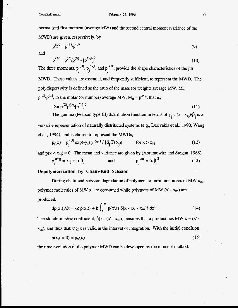
ConKinDegrad February 25, 1996 6
normalized first moment (average MW) and the second central moment (variance of the
MWD) are given, respectively, by
(9)
(10)
payg=p (1) /p (0)
pvx=p (2) /p (0) - [pa"p]2 and
The three moments, p!'), p?, and pjv"', provide the shape characteristics of the jth
MWD. These values are essential, and frequently sufficient, to represent the MWD. The
polydispersivity is defined as the ratio of the mass (or weight) average MW, M, =
~(~)/p( ' ) , to the molar (or number) average MW, Mn = pavg, that is,
J
(1 1) (2) (0) (1) 2 D = p p /[P 1 The gamma (Pearson type III) distribution function in terms of y. = (x - XSj)/P. is a
J J
versatile representation of naturally distributed systems (e.g., Darivakis et al., 1990; Wang
et al., 1994), and is chosen to represent the MWDs,
pj(x> = pj'O' exp(-yj> yjaj-l/ [P. r(a.11 for x 2 Xsj J J
and p(x 5 XSj) = 0. The mean and variance are given by (Abramowitz and Stegun, 1968)
(13) and pjv, = ajpj 2 . = xsj + a.P. pJ J J
Depolymerization by Chain-End Scission
During chain-end-scission degradation of polymers to form monomers of MW Xm,
polymer molecules of MW x' are consumed while polymers of MW (x' - xm) are
produced, 00
dp(x,t)/dt = -k p(x,t) + k p(x',t) 6[x - (x' - x,)] dx'
The stoichiometric coefficient, 6[x - (x' - x,)], ensures that a product has MW x = (x' -
xm>, and thus that X' 2 x is valid in the interval of integration. With the initial condition
p(x,t = 0) = po(x>
the time evolution of the polymer MWD can be developed by the moment method.

ConKinDegrad February 25, 1996 7
The moment operation, applied to Eq (14) and interchanged with the time
derivative, yields ordinary differential equations for moments. The integration order of x
and XI forfie term on the rhs of Eq (14) is interchanged so that m X' W I, dx' p(X',t) J, dx X" 6[X - (x' - xm)] = J, dx' (XI - xm)"p(x',t) (16)
The differential equation for the moments p(")(t), in terms of the binomial coefficient (".) =
n!/(n-j)!j!, becomes J
n
dp(")/dt = -k p(") + k j =O (-l)n-J(nj) x,n-J pti) (17)
with initial conditions, p(")(t = 0) = po(n) For the zero moments (n = 0) we have
(18) dp(O)/dt = 0 or p (0) (t ) = PO(')
Each scission event creates a monomer and a replacement polymer, thus the molar
concentration of polymer is constant. The equation for the fiist moment (n = 1) is
(19) dp (1) /d t=-kxmp (0)
in terms of the the initial first and zero moments, PO(') and p(O). This shows that the
polymer mass concentration decreases linearly in time with rate k x ~ O ( ~ ) . The average
M W decreases with time according to
pavg(t) = poavg - Xm k t (21)
The degradation is complete (conversion is 100 percent) when the polymer mass
approaches zero, i.e., when
tf = /k xm (22)
where poavg >> Xm for a high MW polymer. The second moment equation,
(23) dp (2) /dt = k ~ m * p(O) - 2 k Xm p(')
p(2)(t) = pJ2)+ Xm2 p io) k t (1 + k t) - 2 Xm PO ("k t
has the solution
(24)
One can show that the variance of the MWD thus increases linearly with t,

ConKinDegrad February 25, 1996 8
The monomer MWD, q(x,t), obeys a balance equation with an accumulation and a
generation term,
dq(x,t)/dt = k lxmp(x',t) 6(x - xm) dx'
and the initial condition, q(x,t = 0) = 0. The moment equation can be written
dq(")/dt = k -dx' p(x',t) dx xn 6(x - x,) = k xmn p (0) 0
The solution for any moment is simply
q(@(t) = xmn PO(') k t
Thus the monomer molar concentration increases linearly with time,
q")(t) = PO(') k t
The mass concentration also increases linearly with time,
q(')(t) = Xm PO(') k t
so that the M W of the monomer is constant,
qavg(t> = q"'(t)/q'O)(t> = xm (3 1)
The sum of p(')(t) and q(')(t) is the total mass, which is constant and equal to the initial
polymer mass, PO('). The variance of the monomer MWD is always zero, and thus the
monomer MWD can be written as the Dirac delta function
q(x,t) = q"'(t) 6(x - xm)
We note that the time dependence of all moments is manifested through the dimensionless
variable, kt.
Some of the results in this section for chain-end scission can be derived with a
discrete model beginning with a polymer of given M W (Madras et al., 1996b) and using
summations to formulate the moments. An advantage of the continuous approach is that it
allows consideration of the more realistic initial distribution of reactant polymers. The
interpretation of experimental MWDs for degradation of such polymers (Wang et al., 1995;
Madras et al., 1996a,b) requires a model based on distributions.

ConKinDegrad February 25, 1996
Polymer Degradation by Chain Scission
9
The preceding chain-end scission model is based on i,,e premise that product
monomer-can be distinguished from polymer. For example, gel permeation
chromatography analysis displays a narrow peak for monomer products that is distinct
from the polymer (Madras et al., 1996a,b). The moment approach yields separate
moments, and thus separate peaks, for monomer and polymer. For chain scission of a
polymer, however, the products of the scission are two polymers that are not in general
distinguishable from the reactant polymer. A moment theory that utilizes only the lower (n
= 0, 1,2) moments (e.g., Wang et al., 1995) could be used to reconstruct an evolving
unimodal MWD, but not one that becomes bimodal unless reactant polymer is separate
from product polymer. Bimodal MWDs have been observed for mechanical degradation of
polymer (Price and Smith, 1991). Calculating higher moments and using them in a Gram-
Charlier series to construct complex MWDs could potentially yield bimodal features. The
convergence, however, of such series is slow, and many terms (and higher moments)
would be needed for reliable results. A model is next developed, therefore, that allows the
reactant polymer to be described by its moments, and the products of chain scission to be
described by another set of moments. Each set of moments specifies a MWD whose sum
can be either unimodal or bimodal. The basis for the development is further discussed in
McCoy and Wang (1994).
Degradation with r scissions in sequence can be represented as (McCoy and Wang,
1994) x +(x - x ) + x 2
x2 + (x2 - x3) + x3 1 1 2
or as x1 + (x -x ) + (x -x ) + ... + (xr-l-x> + xr 1 2 2 3 (33)

ConKinDegrad February 25, 1996 10
when all rate constants are equal. The governing balance equations can be written for j = 0, 1, 2, ... , r-1 (with ko = kr = 0)
The moment equations are ordinary differential equations, from which sequential solutions
can be developed for any value of j+l from 1 to r.
The moment operation applied to the term involving fi(x,x') deserves attention.
Substituting the general expression (4) and interchanging x aid XI in the integration yields 00 X'
2 k Jo dx' p(x',t) x'-(2m+l) jo dx xn+m(x' - x)m r(2m+2) / r(m+1)2
= 2 k p("'(t) Znm
where, after expanding (x' - x)m as a binomial sum, we define
z = [r(2m+2) / [r(m+l)2~C(-l)m-J(mj)/(2m+n-j+l) m
j=O nm (37)
Some values of Znm are summarized in Table I. For n = 0 and 1, Znm = 1 or 1/2,
respectively, for all m. The limiting values for the second moments (n=2) are 2, = 1/3
and Z = 1/4. The difference between random- and midpoint-chain scission mechanisms n-
is observed, thus, only for the second moment.
For the batch reactor the moment equations are dp,(")/dt = -kp,(")
nm dp.(")/dt 1 = -kpi(n) + (n) 2kz
and
dpr(")/dt = p r- 1 (n) 2kZ nm
with initial conditions
pi (n) (t=O)=O fori > 1
i = 2, ..., r-1
(38)
(39)
The differential equations have the solutions
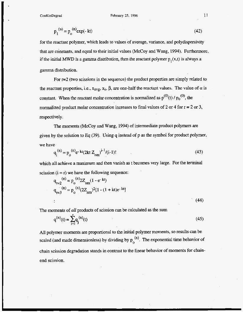
ConKinDegrad February 25, 1996 11
for the reactant polymer, which leads to values of average, variance, and polydispersivity
that are constants, and equal to their initial values (McCoy and Wang, 1994). Furthermore, if the initial MWD is a gamma distribution, then the reactant polymer p,(x,t) is always a
gamma distribution.
For r=2 (two scissions in the sequence) the product properties are simply related to
the reactant properties, i.e., Xavg, xs, p, are one-half the reactant values. The value of a is
constant. When the reactant molar concentration is normalized as p (t) / PO(’), the (0)
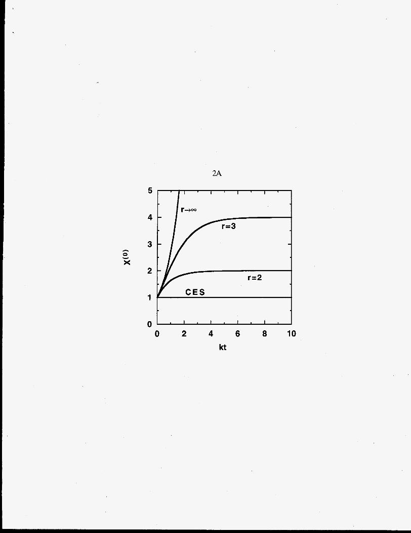
normalized product molar concentration increases to final values of 2 or 4 for r = 2 or 3,
respectively.
The moments (McCoy and Wang, 1994) of intermediate product polymers are
given by the solution to Eq (39). Using q instead of p as the symbol for product polymer,
we have
which all achieve a maximum and then vanish as t becomes very large. For the terminal
scission (i = r) we have the following sequence:
The moments of all products of scission can be calculated as the sum r
q(“)(t) = Cq(n)(t) j=2 J (45)
All polymer moments are proportional to the initial polymer moments, so results can be scaled (and made dimensionless) by dividing by pdn). The exponential time behavior of
chain scission degradation stands in contrast to the linear behavior of moments for chain-
end scission.
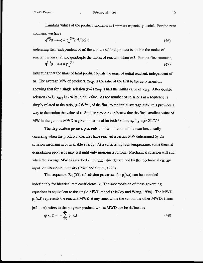
ConKinDegrad February 25, 1996 12
Limiting values of the product moments as t += are especially useful. For the zero
moment, we have
q(o)(t +-> = p0(0)2r-l/(r-2)! (46)
indicating that (independent of m) the amount of f i a l product is double the moles of
reactant when r=2, and quadruple the moles of reactant when -3. For the first moment,
indicating that the mass of final product equals the mass of initial reactant, independent of
m. The average MW of products, Xavg, is the ratio of the fist to the zero moment,
showing that for a single scission (r=2) xavg is half the initial value of xavg. After double
scission (1=3), Xavg is 1/4 its initial value. As the number of scissions in a sequence is
simply related to the ratio, (r-2)!/2r-ly of the final to the initial average MW, this provides a
way to determine the value of r. Similar reasoning indicates that the final smallest value of
MW in the gamma MWD is given in terms of its initial value, G, by x0(r-2)!/2r-1.
The degradation process proceeds until termination of the reaction, usually
occurring when the product molecules have reached a certain MW determined by the
scission mechanism or available energy. At a sufficiently high temperature, some thermal
degradation processes may last until only monomers remain. Mechanical scission will end
when the average M W has reached a limiting value determined by the mechanical energy
input, or ultrasonic intensity (Price and Smith, 1993). The sequence, Eq (33), of scission processes for p.Jx,t) can be extended
indefinitely for identical rate coefficients, k. The superposition of these governing
equations is equivalent to the single-MWD model (McCoy and Wang, 1994). The MWD p,(x,t) represents the reactant MWD at any time, while the sum of the other MWDs (from
j=2 to -) refers to the polymer product, whose MWD can be defined as
(48) j =2
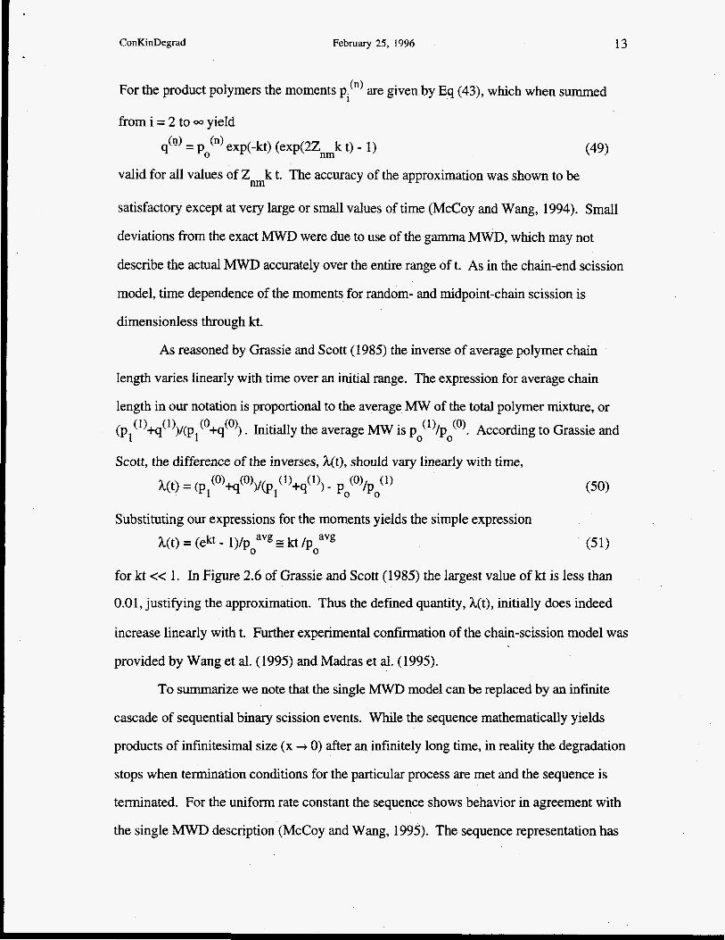
ConKinDegrad February 25, 1996 13
For the product polymers the moments p.'") are given by Eq (43), which when summed
from i = 2 to
1
yield
q(") - - Po exp(-kt) (exp(2Z nm k t) - 1) (49)
valid for all values of Zn,k t. The accuracy of the approximation was shown to be
satisfactory except at very large or small values of time (McCoy and Wang, 1994). Small
deviations from the exact MWD were due to use of the gamma MWD, which may not
describe the actual MWD accurately over the entire range oft. As in the chain-end scission
model, time dependence of the moments for random- and midpoint-chain scission is
dimensionless through kt.
As reasoned by Grassie and Scott (1985) the inverse of average polymer chain
length varies linearly with time over an initial range. The expression for average chain
length in our notation is proportional to the average MW of the total polymer mixture, or (pl (1) q (1) )/(pl (0 +q (0) ) . Initially the average MW is p;')/p:). According to Grassie and
Scott, the difference of the inverses, h(t), should vary linearly with time,
Substituting our expressions for the moments yields the simple expression h(t) = (ekt - l)/p 0 avgz kt /p 0 (51)
for kt << 1. In Figure 2.6 of Grassie and Scott (1985) the largest value of kt is less than
0.0 1, justifying the approximation. Thus the defined quantity, h(t), initially does indeed
increase linearly with t. Further experimental confirmation of the chain-scission model was
provided by Wang et al. (1995) and Madras et al. (1995).
To summarize we note that the single MWD model can be replaced by an infinite
cascade of sequential binary scission events. While the sequence mathematically yields
products of infinitesimal size (x + 0) after an infinitely long time, in reality the degradation
stops when termination conditions for the particular process are met and the sequence is
terminated. For the uniform rate constant the sequence shows behavior in agreement with
the single MWD description (McCoy and Wang, 1995). The sequence representation has

ConKinDegrad February 27, 1996 14
the benefit of allowing a moment procedure to be applied to the separate reactant and
product MWDs. The peaks that are constructed by means of the zero, first, and second
moments are good approximations to the MWD solution.
Results
We illustrate the degradation models by calculations showing how MWDs and their
moments evolve in time. Values of the parameters used in the calculations are based on
Wang et al. (1995): a, = 1.7, Po = 850, xo = 1000, p0(O) = 1/2000. The MW of the
smallest product of degradation (the monomer) is Xm (= 100, the M W of methyl
methacrylate) and is very small relative to the M W s of most polymers. The derived
expressions can all be cast into dimensionless form to reduce the number of parameters that
must be specified. For example, rather than plot time as t, it is convenient to use
dimensionless kt. The total polymer MWD can be monitored as a function of time by gel
permeation chromatography of samples from the polymer mixture. The total polymer MWD for chain scission is p,,,(x,t) = pl(x,t) + q(x,t), and for chain-end scission, p(x,t),
because the monomer product can be distinguished from the polymer reactant. The total
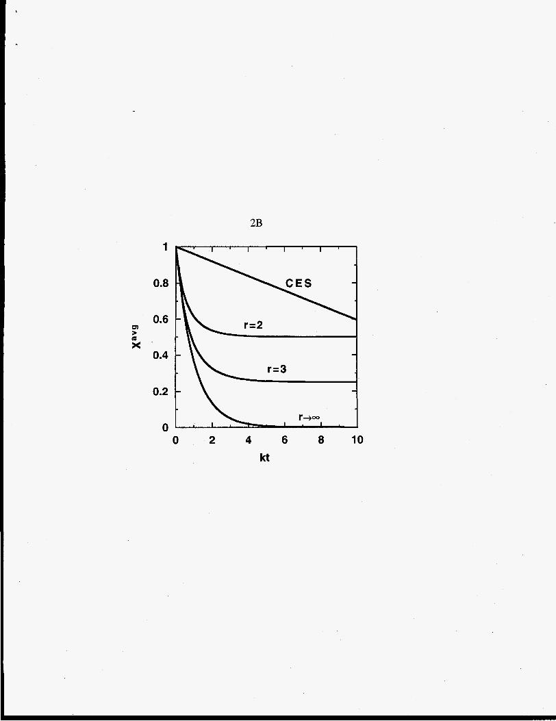
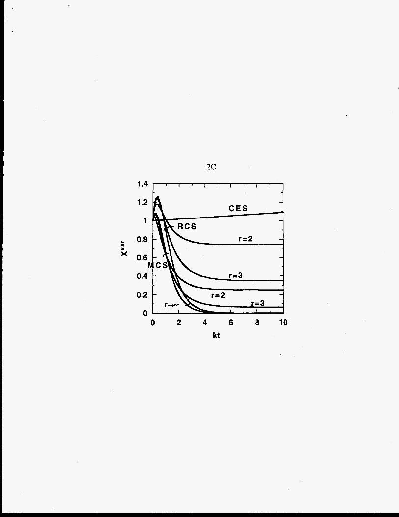
moments are made dimensionless by defining
For chain-end scission (CES) and for random- (RCS) and midpoint-chain scission (MCS),
Figure 2 displays the time dependence of these moments. For chain-end scission the
moments are linear in t, and for random- and midpoint-chain scission the moments behave
exponentially.
The polydispersivity D, Eq (1 l), is graphed in Figure 3 as a function of time for
various cases. As r increases, D increases because smaller MW products are formed by
chain scission.
ConKinDegrad February 25, 1996 15
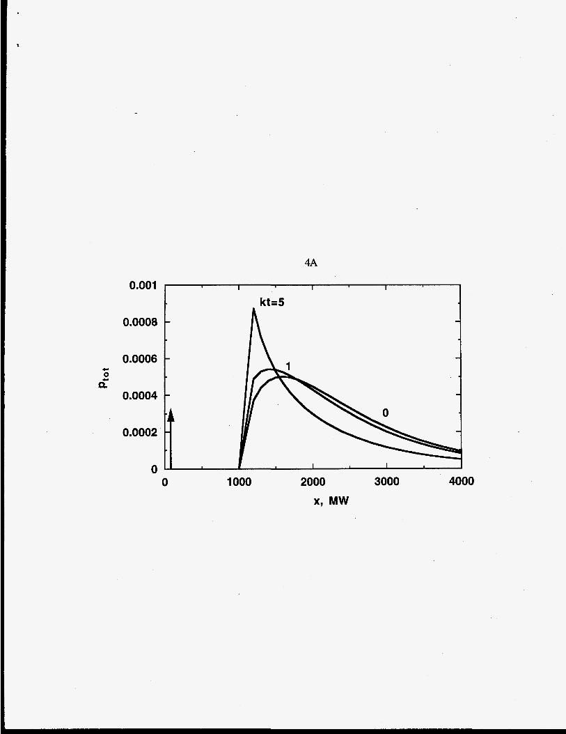
Figures 4 A, B, C show the effect of scission mechanism and the stoichiometric
coefficient parameter m on the time dependence of the polymer MWDs. The reactant and
product MWDs are represented as gamma MWDs and added together for chain scission.
The sum of pl(x,t) and q(x,t) is the total molar MWD, ptot(x,t), which is related to the
mass MWD measured by gel permeation chromatography. The dimensionless MWD is
plotted as ptot(x,t)/po@). Bimodal distributions are evident for all the scission modes.
Chain-end scission (Figure 3A) yields a product monomer that is represented as a delta
function growing in time. The polymer MWD decreases with time. As time approaches tf,
the polymer is entirely consumed and converted to monomer. Midpoint-chain scission with
r=2 (3B), and random-chain scission with r+= (3C) yield product distributions that
increase nonlinearly with time.
The results of the moment analysis of the governing integrodifferential equations
for the MWDs of degrading polymers have obvious implications for data interpretation.
Monitoring the time dependence of the MWDs and their moments provides considerable
information beyond the molecular-weight averages that are typically measured. Such data
allows a sharper interpretation of the kinetics and mechanism of the degradation reactions.
For real polymers and mixtures of polymers, combinations of the mechanisms discussed in
this paper may be operative.
Acknowledgement: The financial support of Pittsburgh Energy Technology Center Grant
No. DOE DE-FG22-94PC94204 and EPA Grant No. CR 822990-01-0 is gratefully
acknowledged.
ConKinDegrad February 27, 1996 16
Literature Cited
Abramowitz, M., I.A. Stegun, Handbook ofMathematica1 Functions, National Bureau of
Standards (1968); Chap. 26.
Aris, R., G.R. Gavalas, "On the Theory of Reactions in Continuous Mixtures," Phil.
Trans. R. SOC. London A260, 351 (1966).
Caeter, P.V., E.J. Goethals, "Telechelic Polymers: New Developments," TRIP 3, 227
(1995).
Clay, P.A., R.G. Gilbert, "Molecular Weight Distributions in Free-Radical
Polymerizations. 1. Model Development and Implications for Data Interpretation,"
Macromolecules 28,552 (1995).
Darivakis, G.S., W.A.Peters, J.B. Howard, "Rationalization for the Molecular Weight
Distributions of Coal Pyrolysis Liquids," AIChE J. 36, 1189 (1990).
Florea, M, "New Use of Size Exclusin Chromatography in Kinetics of Mechanical
Degradation of Polymers in Solution," J. Appl. Polymer Sci. 50,2039 (1993).
Flynn, J.H., R.E. Florin, "Degradation and Pyrolysis Mechanisms," in Pyrolysis and GC
in Polymer Analysis; Leibman, S.A., Levy, E.S., eds; Marcel Dekker Inc., New York,
1985; pp 149-208.
Grassie, N., G. Scott, Polymer Degradation and Stabilisation, Cambridge University
Press, Cambridge, (1985).
Hawkins, W.L., Polymer Degradation and Stabilization, Springer-Verlag, NY ( 1984).
Jellinek, H.H.G., Degradation of Vinyl Polymers, Academic Press, NY (1955).
Laurence, R.L., R. Galvan, M.V. Tirrell, "Mathematical Modeling of Polymerization
Kinetics," in Polymer Reactor Engineering, C . McGreavy (ed.), Blackie Academic and
Professional, London ( 1994).
Madras, G., J.M. Smith, B.J. McCoy, "Effect of Tetralin on the Degradation of Polymer
in Solution," I&EC Research. 34,4222 (1995).
ConKinDegrad February 27, 1996 17
Madras, G., J.M. Smith, B.J. McCoy, "Thermal Degradation of Poly(wMethy1styrene) in
Solution," Polymer Degradation and Stability. (1996a); In Press.
Madras, G., J.M. Smith, B.J. McCoy, "Degradation of PMMA in Solution" (1996b);
submitted.
McCoy, B .J., "Continuous-Mixture Kinetics and Equilibrium for Reversible
Oligomerization Reactions," AZChE J. 39, 1827 (1993).
McCoy, B.J., Tontinuous Kinetics of Cracking Reactions: Thermolysis and Pyrolysis,"
Chem. Eng. Sci. (1996), In press.
McCoy, B.J., M. Wang, "Continuous-mixture fragmentation kinetics: Particle size
reduction and molecular cracking," Chem. Eng. Sci. 49, 3773 (1994).
Miller, A. "Industry invests in reusing plastics," Env. Sci. Tech., 28, 16A (1994).
Prasad, G.N., C.V. Wittmann, J.B. Agnew. T. Sridhar, "Modeling of Coal Liquefaction
Kinetics Based on Reactions in Continuous Mixtures," AZChE J. 32, 1277 (1986).
Price, G.J., P.F. Smith, "Ultrasonic Degradation of Polymer Solutions. 1. Polystyrene
Revisited," Polymer International 24, 159 (1991).
Price, G.J., P.F. Smith, "Ultrasonic Degradation of Polymer Solutions: 2. The Effect of
Temperature, Ultrasound Intensity and Dissolved Gases on Polystyrene in Toluene,"
Polymer 34,4111 (1993).
Wang, M., C. Zhang, J.M. Smith, B.J. McCoy, "Continuous-Mixture Kinetics of
Thermolytic Extraction of Coal in Supercritical Fluid," AZChE J. 40, 13 1 (1994).
Wang, M., J.M. Smith, B.J. McCoy, "Continuous Kinetics for Thermal Degradation of
Polymer in Solution," AZChE J. 41, 1521 (1995).

ConKinDegrad February 27, 1996 18
Notation
D polydispersivity
k - degradation rate coefficient
X
XO
Y
Znm
a. J
parameter in stoichiometric coefficient expression, Q(x,x')
molecular weight distribution (MWD) of polymer
initial molecular weight distribution (MWD) of polymer
the nth moment of p(x,t)
average MW of the MWD p(x,t)
reduced second central moment (variance) of the MWD
MWD for monomer or polymer product of chain scission
the nth moment of q(x,t)
number of scissions in a sequence of events
time
molecular weight
molecular weight of the smallest polymer in an initial MWD
molecular weight of the monomer
dimensionless molecular weight in the gamma distribution
constant in the moment expression for MWD (Table I) 'based on the
stoichiometric coefficient, Q(x,x'). parameter in the gamma distribution
width parameter in the gamma distribution
Dirac delta function of x
stoichiometry coefficient for scission process
ConKinDegrad February 25, 1996 19
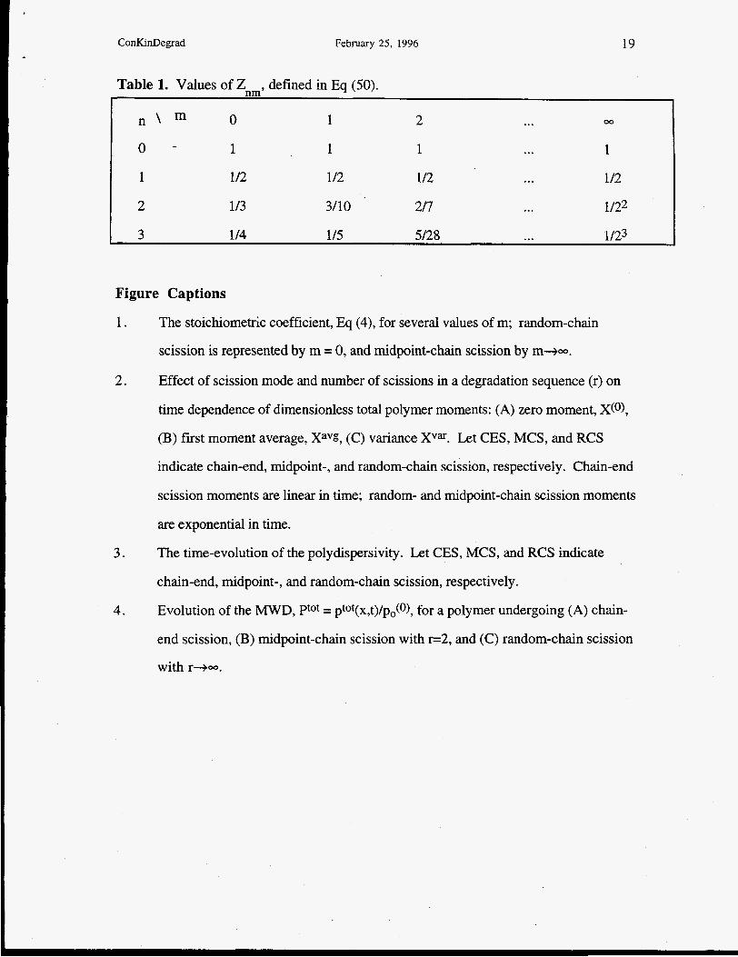
Table 1. Values of Znm, defined in Eq (50). I
1
1
1 112 112 112 ... 112
2 1/3 3/10 217 ... 1/22
3 1 /4 1/5 5/28 ... 1/23
Figure Captions
1. The stoichiometric coefficient, Eq (4), for several values of m; random-chain
scission is represented by m = 0, and midpoint-chain scission by m+-.
2. Effect of scission mode and number of scissions in a degradation sequence (r) on
time dependence of dimensionless total polymer moments: (A) zero moment, X@),
(B) first moment average, XaQ, (C) variance XVX. Let CES, MCS, and RCS
indicate chain-end, midpoint-, and random-chain scission, respectively. Chain-end
scission moments are linear in time; random- and midpoint-chain scission moments
are exponential in time.
The time-evolution of the polydispersivity. Let CES, MCS, and RCS indicate 3.
chain-end, midpoint-, and random-chain scission, respectively.
Evolution of the MWD, Ptot = ptot(x,t)/po(0), for a polymer undergoing (A) chain-
end scission, (B) midpoint-chain scission with r=2, and (C) random-chain scission
with re-.
4.
2
1

1
0 0.25 0.5 0.75 1
x/x'
2A
h 0 v x
0 0 2 4 6 8 10
kt
2B
m > Q X
1
0.8
0.6
0.4
0.2
0 0 2 4 6 8 10
kt
2c
L Q
2
1.4
1.2
1
0.8
0.6
0 2 4 6 8 10 kt

. 3
I ’ I I I I I
0 2 4 6 a 10 kt
t
4A
0.001
0.0008
0.0006
0.0004
0.0002
0
1 1 1
kt=5
t I I /
0 1000 2000 x, MW
3000 4000
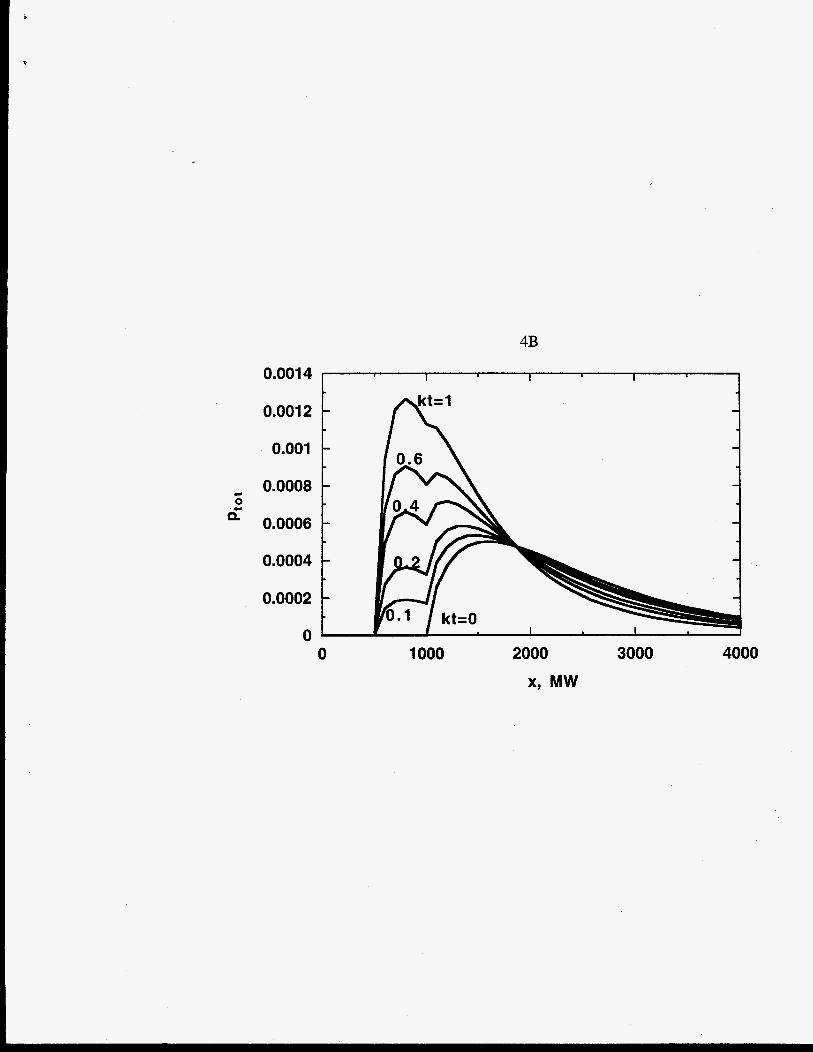
4B
0.0014 I i i i 1
0.001 2
0.001
C 0.0008
0.0006 0 c
0.0004
0.0002
0 0 1000 2000 3000 4000
x, MW

4c
0.001
0.0008
0.0006
0.0004
0.0002
0 0 1000 2000 3000 4000
x, MW