decoupled energy stable schemes for a …shen/pub/lsy14.pdfof two-phase incompressible flows with...

DECOUPLED ENERGY STABLE SCHEMES FOR A PHASE-FIELD MODEL

OF TWO-PHASE INCOMPRESSIBLE FLOWS WITH VARIABLE DENSITY

CHUN LIU\ AND JIE SHEN† AND XIAOFENG YANG‡

Abstract. We consider in this paper numerical approximations of two-phase incompressible flowswith different densities and viscosities. We present a variational derivation for a thermodynami-cally consistent phase-field model that admits an energy law. Two decoupled time discretizationschemes for the coupled nonlinear phase-field model are constructed and shown to be energy stable.Numerical experiments are carried out to validate the model and the schemes for problems withlarge density and viscosity ratios.

1. Introduction

The interfacial dynamics about immiscible and incompressible two-phase flows have attractedmuch attention for more than a century. In recent years, the diffuse interface approaches, orsometimes called phase field models, whose origin can be traced back to [39] and [49], have been usedextensively with much successes and become one of the major tools to study a variety of interfacialphenomena (cf. [24, 5, 31, 26, 30, 54] and the recent reviews [46, 27]). A particular advantageof these phase-field approaches is that they can often be derived from an energy-based variationalformalism (energetic variational approaches), while usually leading to well-posed nonlinear coupledsystems that satisfy thermodynamics-consistent energy dissipation laws. This makes it possibleto carry out mathematical analysis and design numerical schemes which satisfy a correspondingdiscrete energy dissipation law (cf., for instance, [18, 29, 8]). It is a remarkably fact that thenumerical schemes which do not respect the energy dissipation laws may be “overloaded” with anexcessive amount of numerical dissipation near singularities, which in turn lead to large numericalerrors, particularly for long time integration [52, 19, 48, 51, 13]. For the dynamical solutions ofcoarse-graining (macroscopic) process described by the Allen-Cahn and Cahn-Hilliard equations intypical phase-field models that undergo rapid changes and physical singularities at the interface, itis especially desirable to design numerical schemes that preserve the energy dissipation law at thediscrete level.

One of the main challenges in the phase field models is how to describe the dynamics of themixture of two fluids with different densities and viscosities. However, most of the analysis andsimulation of the phase-field models for two-phase flows have been restricted to the cases withmatched density or with small density ratios for which the Boussinesq approximation, where thevariable density is replaced by a background constant density value while an external gravitationalforce is added to model the effect of density difference, can be used (cf. for instance [30]). Whilethe phase-field model with Boussinesq approximation leads to a well-posed dissipative system,their physical validity is based on the assumption that the density ratio between the two phases isrelatively small. Hence, they can not be used for two-phase flows with large density ratios. Thus,

Key words and phrases. Phase-field, two-phase flow, Navier-Stokes, variable density, stability, energy stableschemes.

\Department of Mathematics, Penn State University, University Park, PA 16802 ([email protected]).†Department of Mathematics, Purdue University, West Lafayette, IN 47907 ([email protected]).‡Department of Mathematics, University of South Carolina, Columbia, SC 29208 ([email protected]).

1

2 CHUN LIU & JIE SHEN & XIAOFENG YANG

for the cases with large density ratios, we need to derive physically consistent phase-field modelswhich are also mathematically well-posed.

The challenges and complexities of problems involving the mixtures of different materials lie intheir nature of multiscale and sometimes multiphysics. It is the competitions and couplings betweenthese effects which determine the overall properties of the mixtures. A main difficulty in dealingwith non-matching densities can be seen in the basic macroscopic (continuum) mass conservationρt + div(ρu) = 0 and (macroscopic) incompressibility divu = 0. As the density ρ is an macroscopicquantity, it may be different with the direct average from microscopic descriptions, such as fromthe phase fields. For instance, the mixtures of two incompressible fluids may not be incompressible,for we have to take into consideration of the interaction between two different particles. Variousapproaches have been proposed in the literature. Traditionally, they can be classified into twocategories: incompressible or quasi-incompressible. In the former approach, the volume averagedvelocity is assumed to be incompressible everywhere, including the interfacial region. In the latterapproach, on the other hand, the mass averaged velocity is assumed to satisfy the mass conservationinstead of incompressibility, leading to a slightly compressible mixture inside the interfacial region.In [31], the authors derived a quasi-incompressible phase model which allows the mixture to beslightly compressible inside the interface, see also [1]; a similar quasi-incompressible model, whichadmits an energy law, was proposed recently in [47]. On the other hand, incompressible phase-fieldmodels were derived in [9] and [14], however, these models do not seem to admit an dissipativeenergy law; In [44] and [43], the authors derived incompressible phase-field models, which admitan dissipative energy law, with Allen-Cahn [44] and Cahn-Hilliard [43] dynamics for the cases ofvariable density and viscosity, but the models were derived with an ad-hoc adjustment, whichis mathematically consistent but not frame invariant, on the convection term. In [2], the authorsderived a thermodynamically consistent, which admits an energy law but not frame invariant, diffuseinterface models for incompressible two-phase flows with different densities. Then, they derived in[3] another diffuse interface model which is thermodynamically consistent, frame invariant andadmits an energy law. We want to point out, although all these models are modeling similarproblems of mixtures of two different incompressible fluids, each one of them, including the currentmodel, does have its range of validation and limitations. In particular, all of them can be consideredas an approximation to the sharp interface model.

The first objective of this paper is to rederive the thermodynamically consistent phase-fieldmodel in [2] from an energetic variational point of view.1 The second objective is to design someefficient and accurate numerical schemes for the model which decouple the solution of velocity,pressure, and phase functions. It is particularly challenging to design effective, energy stablenumerical schemes for this system due to the numerous nonlinear couplings. We shall combineseveral approaches which have proved efficient for the phase equations and for the Navier-Stokesequations, namely, the convex splitting (cf. [17, 51, 13]) for the phase equations and projection-typeapproaches [21, 36, 23, 50] for the Navier-Stokes equations. We shall construct two decoupled timediscretization schemes which satisfy a discrete energy law and which lead to, at each time step,a nonlinear elliptic system for the phase function, and a linear elliptic equation for the velocityand pressure respectively. We would like to point out that they appear to be the first schemeswhich decouple the computations of phase function, velocity and pressure, while still preservingthe discrete energy law. In a subsequent paper [45], the technique developed here was used toderive efficient numerical schemes for the model in [3].

The third objective is to validate this model and the proposed numerical schemes through carefulnumerical simulations, including the dynamics of an air bubble rising in water, a particularlychallenging situation where the density ratio is close to 1000 and the viscosity ratio is close to 70.

1After we derived the model independently, we learned that the identical model was already derived in [2].

DECOUPLED ENERGY STABLE SCHEMES FOR A PHASE-FIELD MODEL 3

The rest of the paper is organized as follows. In the next section, we describe the phase-fieldmodel. In Section 3, we provide a detailed energetic derivation for the new model. Then, in Section4, we construct several efficient numerical schemes and prove their stability. In Section 5, weprovide some numerical evidences to validate the new model and the proposed numerical schemes,and summarize our contributions.

2. A Cahn-Hilliard phase-field model with variable density and viscosity

We consider a mixture of two immiscible, incompressible fluids in a confined domain Ω withdensities ρ1, ρ2 and viscosities µ1, µ2, respectively. As usual, we introduce a phase function(macroscopic labeling function) φ such that

φ(x, t) =

1 fluid 1,

−1 fluid 2,(2.1)

with a thin, smooth transition region of width O(η). The (equilibrium) configurations and patternsof this mixing layer, in the neighborhood of the level set Γt = x : φ(x, t) = 0, is determined bythe microscopic interactions between fluid molecules. For the isotropic interactions, the classicalself consistent mean field theory (SCMFT) in statistical physics [11] yields the following Ginzburg-Landau type of Helmholtz free energy functional:

W (φ,∇φ) =

∫Ωλ(

1

2|∇φ|2 + F (φ))dx,(2.2)

where the first term contributes to the hydro-philic type (tendency of mixing) of interactionsbetween the materials and the second part, the double well bulk energy F (φ) = 1

4η2(φ2 − 1)2,

represents the hydro-phobic type (tendency of separation) of interactions. As the consequence ofthe competition between the two types of interactions, the equilibrium configuration will include adiffusive interface with thickness proportional to the parameter η (cf., for instance, [54]); and, as ηapproaches zero, we expect to recover the sharp interface separating the two different materials.

The hydrodynamics of this mixture can be viewed as an isothermal system governed by theenergetic variational approaches for general dissipative systems. The combinations of the FirstLaw of Thermodynamics and the Second Law of Thermodynamics gives:

d

dtEtotal = −∆,(2.3)

where Etotal is the sum of kinetic energy and the total Helmholtz free energy, and ∆ is the entropyproduction (energy dissipation rate in this case). All the physical ingredients, assumptions, aswell as limitations of the system are included in the expressions of the total energy functional andthe dissipation functional, and the kinematic (transport) relation of the variables employed in thesystem.

The hydrodynamics of the mixtures, by nature, is a multiscale problem. The competition ofthe macroscopic flow properties and the microstructures due to the molecular interactions gives allthe intriguing and complicated behaviors of the systems. In fact, the choices of the variables andalso the specific physics, in terms of the energetic functionals, demonstrated the specific physicalsituations or applications in consideration.

In this paper, we are interested in the overall macroscopic flow properties, which self-consistentlytake into account the microscopic properties of the mixtures. For this purpose, we consider thesystem with the following total energy:

E(φ,∇φ) =

∫Ω

(ρ(φ)

1

2|u|2 + λ(

1

2|∇φ|2 + F (φ))

)dx.(2.4)


It is clear that the first term is the macroscopic kinetic energy. The second part, the coarse grainedinternal energy, includes the competition between the hydro-philic and hydro-phobic interactionsbetween two different ingredients. The constant λ represents the competition between the kineticenergy and the total internal energy, and can be directly related to the commonly known surfacetension constant [54].

The dynamics of the phase function include both the macroscopic kinematic transport relationand also the long-time microscopic dissipations: φ by the following Cahn-Hilliard gradient flow (cf.[10, 24, 5, 31, 26, 30]):

φt + (u · ∇)φ = −M∆w,

w :=δE

δφ= λ(∆φ− f(φ))− ρ′(φ)

|u|2

2,

(2.5)

where w is the so called chemical potential and M is a mobility constant related to the relaxationtime scale, and f(φ) = F ′(φ). The right-hand side of the equation for φ is the coarse grained formof the microscopic dissipation (general diffusion) relation.

The momentum equation (macroscopic force balance) for the whole system takes the usual form:

ρ(ut + (u · ∇)u) = ∇ · τ,(2.6)

where the total stress τ = µD(u) − pI + τe with D(u) = ∇u + ∇uT and τe is the extra elasticstress induced by the microscopic internal energy. It will be shown in the next section, by a unifiedenergetic variational approach, that the momentum equation becomes:

ρ(ut + (u · ∇)u) = ∇ · (µD(u)− pI − λ∇φ⊗∇φ),(2.7)

where p includes both the hydrostatic pressure due to the incompressibility and also the contribu-tions from the induced stress.

In the above, ρ and µ are slave variables of φ, which can be defined, for example, as

(2.8) ρ(φ) =1 + φ

2ρ1 +

1− φ2

ρ2, µ(φ) =1 + φ

2µ1 +

1− φ2

µ2.

Without loss of generalities, we consider the boundary conditions

u|∂Ω = 0,∂φ

∂n|∂Ω = 0,

∂w

∂n|∂Ω = 0.(2.9)

The Cahn-Hilliard phase equation (2.5) and the momentum equations (2.7) with the boundarycondition (2.9), together with the incompressibility constraint

(2.10) ∇ · u = 0,

form a closed system for the particular set of variables of our choice for this study, (u, p, φ, w), andwith the auxiliary variable ρ and µ given by (2.8).

Direct computation shows that, even in cases of ρ1 6= ρ2, the Cahn-Hilliard phase-field system(2.5)-(2.7)-(2.10) still admits the following energy law:

d

dt

∫Ω

(1

2ρ(φ)|u|2 +

λ

2|∇φ|2 + λF (φ))dx = −

∫Ω

(µ2|D(u)|2 +M |∇w|2

)dx.(2.11)

While the left-hand side includes all the physics we want to discuss in this system, the macroscopichydrodynamics and the microscopic mixing, the right-hand side represents dissipation mechanismsfrom both scales. The viscosity term, the first term on the right-hand side, represents the macro-scopic dissipation, and the second term stands for the microscopic internal damping during themixing.


3. The energetic variational derivation of the system

The complicated mechanical and rheological properties of the coupled system derived in the lastsection can be attributed to the competitions and couplings between different parts of the totalenergy functionals (in this case, the kinetic energy and the free energy) and different parts of thedissipation (the viscosity and the internal dissipation of the microstructure). One issue we want topoint out is the kinematic assumptions involved in the system.

The energy dissipation law (2.11) is consistent with the second law of thermodynamics. Sincewe only consider the isothermal situation here, the total dissipation in the right hand side of (2.11)is equal to the total entropy production. The left-hand side is the total energy, which is the sumof kinetic energy plus the (Helmholtz) free energy.

In order to obtain the force balance equations from the general dissipation law (2.3), we employthe Least Action Principle (LAP) for the Hamiltonian part of the system and the Maximum Dis-sipation Principle (MDP) for the dissipative part. Formally, LAP just states the fact that forcemultiplies distance is equal to the work, i.e.,

δE = force× δx,(3.1)

where x is the position, δ is the variation (derivative) in general senses. This procedure will givethe Hamiltonian part of the system and the conservative forces [6, 4]. On the other hand, MDP,by Onsager and Rayleigh [38, 33, 34], yields the dissipative forces of the system:

δ1

2∆ = force× δx.(3.2)

Here the factor 12 is consistent with the choice of quadratic form of the “rates”, which in turn

describes the linear response theory for long-time near equilibrium dynamics [28].As we discussed before, the system (2.5)-(2.7)-(2.10) is a multi-scale/multi-physics system. The

hydrodynamic equation (2.7) describes the macroscopic (continuum) force balance, while the dy-namic equation (2.5) for the phase field φ describes the evolution of microstructures due to themixing of two materials.

Let us start with the equation (2.5). Here we introduce the free energy functional, which isthe consequences of various coarse graining process, such as the self-consistent mean field theory(SCMFT):

(3.3)

∫Ωλ(

1

2|∇φ|2 + F (φ))dx.

Energetically, this “mixing” energy determines the equilibrium configuration of the mixing. Thepresence of the gradient term gives rise the spatial microstructures.

In order to describe the effect of the macroscopic flow field u(x, t) to the microstructure, weintroduce the kinematic transport relation:

(3.4)D

Dtφ(x, t) = φt + u · ∇φ = 0.

This relation can also be interpreted as the immiscibility of the mixing, which is independent tothe energetic descriptions of the system. This kinematic assumption on φ demonstrates the natureof φ being a label function, satisfying

(3.5) φ(x(X, t), t) = φ0(X),

where, as usual, X and x represent the Lagrangian and Eulerian coordinates, respectively, andx(X, t) is the flow map such that xt(X, t) = u(x(X, t), t), x(X, 0) = X. Hereafter, the spatialderivation without sub-index represents derivative with respect to Eulerian coordinates x, whilethe derivatives with respect to the Lagrangian coordinates X will be marked out specifically.


We want to point out that, in order to describe the deformation or evolution of configurationsor patterns, one needs to introduce the deformation tensor F = ∂x

∂X . The usual (macroscopic)incompressible condition

(3.6) ∇ · u = 0,

is the direct consequence of the constraint det(F ) = 1 and the algebraic identity δdet(F ) =det(F ) tr(F−1δf).

For constant mobility M , the Cahn-Hilliard dynamics (2.5) can be viewed as a relaxation ap-proximation to (3.4), formally by letting M approaches zero. On the other hand, from the energydissipation law (2.11), the second term in the right hand side represents the microscopic internaldissipation. From there, one can derive the Cahn-Hilliard dynamics, as a general diffusion mecha-nism, represents the long-time, near equilibrium behavior for the microscopic time scale. It can alsobe regarded as the microscopic relaxation (in time) of the microstructures, hence the microscopicforce balance.

Now, we want to derive the macroscopic force balance equation (2.7). To this end, we start withthe reversible part of the system. From the total energy of the left-hand side of (2.11), we candefine the action function, after the Legendre transformation [7], in terms of the volume preservedflow map x(X, t):

A(x) =

∫ ∫(1

2ρ(φ)|u|2 − λ

2|∇φ|2 − λF (φ)) dxdt(3.7)

=

∫ ∫(1

2ρ(φ0)|xt|2 −

λ

2|F−1∇Xφ0(X)|2 − λF (φ0)) dXdt.

The first equality is obtained by taking the Legendre transform of the total energy functional withrespect to u, which gives the negative sign between the kinetic energy and the free energy. Thesecond equality is derived from the volume preserving constraint (incompressibility, i.e., det(F ) = 1)of the flow map and the kinematic assumption of φ in (3.4) (the transport part of (2.5)).

Suppose there is a one-parameter family of these flow map xε(X, t), with x0(X, t) = x, andddεx

ε(X, t)|ε=0 = y(X, t). From the volume preserving constraint det∂xε

∂X = 1, it is easy to showthat, if y(x(X, t), t) = y(X, t), one can derive from the algebraic identity of the derivatives of thedeterminants that:

∇ · y = 0.

Taking the variation of A(x) with respect to these volume preserving flow map for arbitrary givendivergence free y, we arrive at the variational (weak) form:∫ ∫

(ρ(φ0(X))(xt, yt)− λ(F−1∇Xφ0(X),−F−1∇XyF−1∇Xφ0(X)) dXdt(3.8)

=

∫ ∫(−ρ(φ0(X))(xtt, y)− λ(F−1∇Xφ0(X),−F−1∇XyF−1∇Xφ0(X)) dXdt

=

∫ ∫−(ρ(φ)(ut + u · ∇u, y) + λ(∇φ,∇y∇φ) dxdt.

Integrating by part and using the fact that y is divergence free, we obtain the macroscopic reversiblepart of (2.7):

ρ(φ)(ut + (u · ∇)u) = −p1I − λ∇φ⊗∇φ,(3.9)

where p1 is the Lagrangian multiplier for the constraint on the volume preserving flow map x(X, t),i.e., ∇ · y = 0.

We want to point out that, while for the case of equal density, we have

ρ(φ)(ut + u · ∇u) = (ρ(φ)u)t + u · ∇(ρ(φ)u),


but this is no longer true when the densities are not the same, as in our situation. Hence we willneed to take the weak form as in (3.8).

Since the macroscopic dissipation in the system is attributed to the viscosity term:∫Ω

µ

2|D(u)|2 dx,

by taking the derivative of the corresponding term in the dissipation with respect to u (Onsager’sMaximum Dissipation Principle), we obtain the dissipative part of the (2.7):

0 = ∇ · (µD(u)− p2I),(3.10)

where p2 is the Lagrangian multiplier for the incompressibility constraint ∇ · u = 0.The final equation (2.7), the total force balance equation, is just the sum of the two parts. Hence,

the total pressure is p = p1 + p2, both represent the Lagrangian multiplier of the incompressibility,one is from the Lagrangian description and the other from the Eulerian formulation.

4. Energy stable time discretizations and their stability analysis

In this section, we design some time discretizations of the new phase-field model (2.5)-(2.7)-(2.10)introduced in the last section. The goal is to construct time discretization schemes which satisfy adiscrete energy dissipation law that is similar to the continuous energy law of (2.11), and are easyto implement in practice.

Let us first reformulate (2.5) and (2.7) into some equivalent forms which are more convenient fornumerical approximation. By using the following identities

∇ · (∇φ⊗∇φ) = ∆φ∇φ+1

2∇|∇φ|2,(4.1)

∇p+ λ∇ · (∇φ⊗∇φ) = ∇(p+1

2λ|∇φ|2 + λF (φ) + φw)− φ∇w +

1

2ρ′(φ)|u|2∇φ.(4.2)

and denoting the modified pressure as p = p + 12λ|∇φ|

2 + λF (φ + φw) (still denote it by p forsimplicity), the system (2.5)-(2.7)-(2.10) can be rewritten as follows:

φt +∇ · (uφ) +M∆w = 0,(4.3a)

w +1

2ρ′(φ)|u|2 − λ(∆φ− f(φ)) = 0,(4.3b)

ρ(φ)(ut + (u · ∇)u)−∇ · µ(φ)D(u) +∇p− φ∇w +1

2ρ′(φ)|u|2∇φ = 0,(4.3c)

∇ · u = 0,(4.3d)

where ρ(φ) and µ(φ) are given by (2.8), and the boundary conditions for (φ,w, u) are given in (2.9).The above coupled nonlinear system presents formidable challenges for algorithm design, analysis

and implementation that we will address in this paper. In this section, we will design numericalalgorithms which admit a discrete energy dissipation law and overcome three main difficultiesassociated with this coupled nonlinear system that are described as follows.

• The coupling between the phase function, chemical potential and the velocity. It appearsvery difficult to decouple the computation of φ and w from the velocity u while the simpleexplicit treatment in the convection term of (4.3a) will not lead to any energy dissipationlaw.• The pressure solver with large density ratio. A common strategy to decouple the compu-

tation of the pressure from velocity is to use a projection type scheme as in the case forNavier-Stokes equations (cf., for instance, a recent review in [23]). However, In the usualprojection type schemes, the subsystem to determine a pressure approximation if often anelliptic equation with 1

ρ as variable coefficient, making it difficult to solve when the density


ratio is large. The additional difficulty is that it is not easy to construct a second-orderscheme based on a pressure-correction formulation (cf. [22]). Thus, we will consider a pres-sure stabilized formulation to avoid solving a pressure elliptic equation with density as avariable coefficient.• The stiffness associated with the interfacial width η. To alleviate the difficulty associated

with the stiffness caused by the thin interfacial width, we can introduce a stabilizing termin the phase equation as in [43, 44, 42, 53]. An alternative way adopted in this paper isto use the idea of convex splitting that was first introduced by Eyre [17]. Recently, theidea has been applied to various gradient flow [51, 13], which serves as inspirations for thenumerical schemes we present below.

We will first construct numerical schemes based on a gauge-Uzawa formulation [32, 15, 36, 43, 15].These schemes require solving an elliptic equation for pressure with the variable coefficient 1

ρ . Then,

we will construct numerical schemes based on a pressure-stabilized formulation [37, 41, 21, 23] whichonly require solving a Poisson equation for pressure.

We assume that we can split F (φ) as Fc(φ) − Fe(φ) with both Fc and Fe being convex, i.e.,F ′′c (φ), F ′′e (φ) ≥ 0. For example, we can take Fc(φ) = φ4 and Fe(φ) = 2φ2 − 1. In what follows, wedenote

f(φ) = F ′(φ), fc(φ) = F ′c(φ), fe(φ) = F ′e(φ).

Without loss of generality, we assume 0 < ρ1 ≤ ρ2 and 0 < µ1 ≤ µ2.

4.1. Schemes based on a gauge-Uzawa formulation. We construct a first-order gauge-Uzawascheme for the phase-field model (4.3) as follows.

Given initial conditions φ0, w0, s0 = 0, u0, we compute (φn+1, wn+1, un+1, un+1, sn+1) for n ≥ 0by

1

δt(φn+1 − φn) +∇ · ((un + δt

φn∇wn+1

ρ(φn+1))φn) +M∆wn+1 = 0,

wn+1 +1

2ρ′(φn+1)|un|2 − λ(∆φn+1 − fc(φn+1) + fe(φ

n)) = 0,

∂nφn+1|∂Ω = 0, ∂nw

n+1|∂Ω = 0;

(4.4a)

ρ(φn+1)un+1 − un

δt+ ρ(φn+1)(un+1 · ∇)un+1 +

1

2ρ(φn+1)(∇ · un+1)un+1

−∇ · µ(φn)D(un+1) + µmin∇sn − φn∇wn+1

+1

2ρ′(φn+1)|un+1|2∇φn+1 = 0,

un+1|∂Ω = 0;

(4.4b)

−∇ · (1

ρ(φn+1)∇ψn+1) = ∇ · un+1,

∂nψn+1|∂Ω = 0;

(4.4c)

un+1 = un+1 +1

ρ(φn+1)∇ψn+1,

sn+1 = sn −∇ · un+1;

(4.4d)


with

ρ(φ) = (φ+ 1)2ρ1/4 + (φ− 1)2ρ2/4, µ(φ) = (φ+ 1)2µ1/4 + (φ− 1)2µ2/4,(4.4e)

and µmin = minµ(φ) > 0.Several remarks are in order.

Remark 4.1. An additional stabilizing term, ρ(φn+1)un

2 ∇ · un+1, is added in (4.4b). This term

does not bring any inconsistency to the governing PDE system (4.3c) because the term ρu2∇ · uvanishes in the PDE level from the incompressibility.

Remark 4.2. The computations of (φn+1, wn+1), un+1, ψn+1 and (un+1, sn+1) are totally decou-pled! We believe, to the best of our knowledge, that this is the first scheme for two-phase flowswhich is both totally decoupled and unconditionally stable (see below).

Remark 4.3. Note that a first order term, δtφn∇wn+1

ρ(φn+1), is added to the convective velocity un in

(4.4a). Hence, the above scheme is formally a first-order approximation to the system (4.3).

Remark 4.4. Since φ should take the values ±1 except at the interfacial region, so if we ignorethe mass conservation for the mixture inside the interfacial region, the form of ρ(φ) and µ(φ) canbe quite flexible. We choose to define ρ in (4.4e) (resp. µ) as the parabolic average of ρ1 and ρ2

(resp. µ1 and µ2) which satisfies

(4.5) ρ′′(φ) > 0 and ρmin = minφ∈Rρ(φ) > 0.

Remark 4.5. In the above scheme, sn is the so called gauge variable, and a proper pressureapproximation is (cf. [36]):

pn+1 = −ψn+1

δt+ µmins

n+1.(4.6)

We also derive from (4.4c)-(4.4d) that divun+1 = 0.

Remark 4.6. Given the data at the n-th level, (4.4a) is an quasilinear elliptic system. Note thatthe special choice of the “average” for ρ(φ) in (4.4e) prevents (4.4a) from developing singularity.Thus, the existence of a solution to this system follows from the standard elliptic theories (see forinstance the standard references in [16, 20]). We will outline the main arguments here for thereaders’ convenience.

We will use the Holder spaces here. Similar arguments can also be extended to other functionalspaces, such as Hilbert-Soblev spaces.

Assuming φn, wn ∈ C1,α for some 0 < α < 1, we will apply the Leray-Schauder fixed pointtheorem to the system (4.4a). Consider the following system with a parameter σ ∈ [0, 1]:

σ 1

δt(φ− φn) +∇ · ((un + δt

φn∇wρ(φ)

)φn)−Mw+M(1 + ∆)wn+1 = 0,

σw +1

2ρ′(φ)|un|2 − λ(−fc(φ) + fe(φ

n)) + λφ − λ(1 + ∆)φn+1 = 0,

∂nφn+1|∂Ω = 0, ∂nw

n+1|∂Ω = 0.

(4.7)

For any fixed σ ∈ [0, 1], the above system defines an operator Tσ(φ,w) = (φn+1, wn+1) : C1,α ×C1,α → C1,α × C1,α. One can readily check that this operator possess the following properties:

• For σ = 0, the system only has an unique solution φn+1 = wn+1 = 0.• For any fixed σ, and arbitrary φ,w ∈ C1,α, from the Schauder estimates of linear elliptic

equations (see for instance, Theorem 2.40 in [16] for a more general statement), one canshow that the solution of (4.7) φn+1, wn+1 ∈ C2,α, which is compactly embedded in C1,α

[25]. Hence, Tσ is a compact operator.


• Thanks to the a-priori Holder estimates for quasilinear elliptic equations [20], one can showthat all fixed points of Tσ are uniformly bounded in C1,α × C1,α.

With these properties, the Leray-Schauder fixed point theorem [20] asserts that the operator Tσ withσ = 1) possess a fixed point (φn+1, wn+1), which is a solution of the original system (4.4a).

Remark 4.7. The equation (4.4b) is also an quasilinear elliptic system. By using a similar argu-ment as above, one can also show that there exists at least one solution for (4.4b).

Theorem 4.1. Solutions to the scheme (4.4) satisfy the following discrete energy law for anyδt > 0:

1

2‖σn+1un+1‖2 + λ

(1

2‖∇φn+1‖2 + (F (φn+1), 1)

)+

1

2µminδt‖sn+1‖2 + δt

(M‖∇wn+1‖2 +

1

2µmin‖∇un+1‖2

)+

1

2‖ 1

σn+1∇ψn+1‖2

≤ 1

2‖σnun‖2 + λ

(1

2‖∇φn‖2 + (F (φn), 1)

)+

1

2µminδt‖sn‖2,

where σn+1 =√ρ(φn+1).

Proof. Let us denote

(4.8) un? = un + δtφn∇wn+1

ρ(φn+1).

We first take the inner product of (4.4b) with 2δtun+1. For the nonlinear terms, we have

(1

2ρ′(φn+1)|un+1|2∇φn+1, un+1) + (ρ(φn+1)un+1 · ∇un+1 +

1

2(∇ · un+1)ρ(φn+1)un+1, un+1)

= (un+1,∇(ρ(φn+1)|un+1|2

2)) +

1

2((∇ · un+1)ρ(φn+1)un+1, un+1) = 0.

Hence, noticing that

ρ(φn+1)un+1 − un

δt− φn∇wn+1 = ρ(φn+1)

un+1 − un?δt

,

using the identity

(4.9) (a− b, 2a) = |a|2 − |b|2 + |a− b|2,and (4.9), we obtain

‖σn+1un+1‖2 − ‖σn+1un?‖2 + ‖σn+1(un+1 − un? )‖2

+ δt‖√µnD(un+1)‖2 + 2µminδt(∇sn, un+1) = 0.

(4.10)

Using (4.4d) and the fact that divun+1 = 0, we derive

(σn+1un+1, σn+1un+1) = (ρ(φn+1)un+1, un+1) = (ρ(φn+1)(un+1 +1

ρ(φn+1)∇ψn+1), un+1)

= (ρ(φn+1)un+1, un+1)

= (ρ(φn+1)un+1, un+1 +1

ρ(φn+1)∇ψn+1)

= ‖σn+1un+1‖2 + (un+1 − 1

ρ(φn+1)∇ψn+1,∇ψn+1)

= ‖σn+1un+1‖2 − ‖ 1

σn+1∇ψn+1‖2,

(4.11)


and

2µminδt(∇sn, un+1) = 2µminδt(sn,−∇ · un+1) = 2µminδt(s

n, sn+1 − sn)

= µminδt(‖sn+1‖2 − ‖sn‖2 − ‖sn+1 − sn‖2)

= µminδt(‖sn+1‖2 − ‖sn‖2)− µminδt‖∇ · un+1‖2.(4.12)

It is easy to check by integration by parts that

‖D(u)‖2 = ‖∇u‖2 + ‖∇ · u‖2, ∀u ∈ H10 (Ω)d.(4.13)

From µmin ≤ µn, we obtain

µmin‖∇ · un+1‖2 + µmin‖∇un+1‖2 = ‖√µminD(un+1)‖2 ≤ ‖√µnD(un+1)‖2.(4.14)

Combining the above inequalities, we arrive at

‖σn+1un+1‖2 − ‖σn+1un?‖2 + ‖ 1

σn+1∇ψn+1‖2 + ‖σn+1(un+1 − un? )‖2

+ µminδt(‖sn+1‖2 − ‖sn‖2) + µminδt‖∇un+1‖2 ≤ 0.(4.15)

From (4.8), we have

ρ(φn+1)un? − un

δt= φn∇wn+1.(4.16)

By taking the inner product of (4.16) with 2δtun? , we obtain

‖σn+1un?‖2 − ‖σn+1un‖2 + ‖σn+1(un? − un)‖2 = 2δt(φn∇wn+1, un? ).(4.17)

Next, taking the inner product of the first equation of (4.4a) with −2δtwn+1, we obtain

−2(φn+1 − φn, wn+1)− 2δt((∇ · (un?φn), wn+1) + 2Mδt‖∇wn+1‖2 = 0.(4.18)

By integration by parts, we have

−((∇ · (un?φn), wn+1) = (φn∇wn+1, un? ).(4.19)

On the other hand, we derive from Taylor expansion that

(4.20) ρ(φn+1)− ρ(φn) = ρ′(φn+1)(φn+1 − φn)− 1

2(ρ′′(ξn)(φn+1 − φn), φn+1 − φn).

Next, by taking the inner product of the second equation in (4.4a) with 2(φn+1 − φn), after usingthe above relation and the fact that ρ′′(ξn) > 0 (cf. (4.5)), we obtain

2(wn+1, φn+1 − φn) + ‖σn+1un‖2 − ‖σnun‖2

+ λ(‖∇φn+1‖2 − ‖∇φn‖2 + ‖∇φn+1 −∇φn‖2)

+ 2λ(fc(φn+1)− fe(φn), φn+1 − φn) ≤ 0.

(4.21)

In order to deal with the nonlinear terms, we obtain the following identities by Taylor expansion,

fc(φn+1)(φn+1 − φn) = Fc(φ

n+1)− Fc(φn) + F ′′c (ξ)(φn+1 − φn)2,

fe(φn)(φn+1 − φn) = Fe(φ

n+1)− Fe(φn)− F ′′e (ζ)(φn+1 − φn)2.(4.22)

Subtracting the second identity from the first one, we find

(fc(φn+1)− fe(φn), (φn+1 − φn)) = (F (φn+1)− F (φn), 1) + (F ′′c (ξ) + F ′′e (ζ))‖φn+1 − φn)‖2

≥ (F (φn+1)− F (φn), 1).(4.23)


Finally, by combining (4.9), (4.15), (4.17),(4.18), (4.21) and (4.23) , we arrive at

‖σn+1un+1‖2 − ‖σnun‖2 + ‖σn+1(un+1 − un? )‖2 + ‖σn+1(un? − un)‖2

+ µminδt(‖sn+1‖2 − ‖sn‖2) + µminδt‖∇un+1‖2 + ‖ 1

σn+1∇ψn+1‖2

+ 2Mδt‖∇wn+1‖2 + λ(‖∇φn+1‖2 − ‖∇φn‖2 + ‖∇φn+1 −∇φn‖2)

+ 2λ(F (φn+1)− F (φn), 1) ≤ 0.

We can then conclude from the above inequality.

Remark 4.8. As noted before, a first-order stabilizing term, −δtwn+1∇φnρ(φn+1)

, is added to the convective

velocity un in (4.4a). This term can not be replaced by a second-order stabilizing term while main-taining the unconditional stability. However, one may construct efficient decoupled linear schemesat the expense of unconditional stability. For example, a formally second-order, decoupled linearscheme is as follows:

For the sake of simplicity, we shall denote, for any sequence ak, a∗,k+1 = 2ak − ak−1.

3φn+1 − 4φn + φn−1

2δt+∇ · (u∗,n+1φ∗,n+1) +M∆wn+1 = 0,

wn+1 +1

2ρ′(φ∗,n+1)|u∗,n+1|2 +

1

η2(φn+1 − 2φn + φn−1)

+ λ(−∆φn+1 + 2f(φn)− f(φn−1)) = 0,

∂nφn+1|∂Ω = 0, ∂nw

n+1|∂Ω = 0;

(4.24a)

ρ(φn+1)3un+1 − 4un + un−1

2δt+ ρ(φn+1)(u∗,n+1 · ∇)u∗,n+1

−∇ · µ(φn+1)D(u∗,n+1) +∇pn + µmin∇sn

− φ∗,n+1∇wn+1 +1

2ρ′(φn+1)|u∗,n+1|2∇φ∗,n+1 = 0,

un+1|∂Ω = 0;

(4.24b)

−∇ · (1

ρ(φn+1)∇ψn+1) = ∇ · un+1

∂nψn+1|∂Ω = 0;

(4.24c)

un+1 = un+1 +

1

ρ(φn+1)∇ψn+1,

sn+1 = sn −∇ · un+1,

pn+1 = pn − 3

2δtψn+1 + µmins

n+1,

(4.24d)

with ρ(φ) and µ(φ) defined in (4.4e) and µmin = minµ(φn+1) > 0.The above scheme is much easier to implement than the scheme (4.4). More precisely, at each

time step, it involves a coupled linear system with constant coefficients for (φn+1, wn+1), and anelliptic equation for un+1 and ψn+1, respectively.


4.2. Schemes based on a pressure-stabilization formulation. We observe that for problemswith large density ratios, the elliptic equation (4.4c) for pressure maybe difficult and time consuming(often consuming more than 90% of the total cost) to solve compared with a Poisson equation.Therefore, we will design a pressure-stabilized formulation which only requires solving a Poissonequation for the pressure [23, 44].

Therefore, we now construct schemes based on the pressure-stabilization formulation (cf., forinstance, [37, 41, 35, 21]), namely, the divergence free condition is replaced by

(4.25) ∇ · u− ε∆pt = 0,

where ε is a small parameter.Inspired by the schemes presented in [23, 43], the first order pressure-stabilization scheme is

given as follows.Given initial conditions φ0, p0 = 0, u0, we update (φn+1, un+1, pn+1) for n ≥ 0 by

1

δt(φn+1 − φn) + (un + δt

φn∇wn+1

ρ(φn+1)) · ∇φn +M∆wn+1 = 0,

wn+1 +1

2ρ′(φn+1)|un|2 − λ(∆φn+1 − fc(φn+1) + fe(φ

n)) = 0,

∂nφn+1|∂Ω = 0, ∂nw

n+1|∂Ω = 0;

(4.26a)

ρ(φn+1)

un+1 − un

δt+ ρ(φn+1)(un+1 · ∇)un+1 +

1

2ρ(φn+1)(∇ · un+1)un+1

−∇ · µ(φn)D(un+1) +∇(2pn − pn−1)− φn∇wn+1 +1

2ρ′(φn+1)|un+1|2∇φn+1 = 0,

un+1|∂Ω = 0;

(4.26b)

∆(pn+1 − pn) =ρ

δt∇ · un+1,

∂npn+1|∂Ω = 0;

(4.26c)

with ρ(φ), µ(φ) as defined in (4.4e) and ρ = 12minρ(φn+1) > 0.

Several remarks are in order.

Remark 4.9. The stabilizing term ρ(φn+1)un+1

2 ∇·un+1, formerly with order O(δt2) in the discrete

level thanks to (4.26c), that vanishes in the PDE level from the incompressibility, is added in(4.26b).

Remark 4.10. As for the scheme (4.4), the above scheme consists of three decoupled steps for(φn+1, wn+1), un+1 and pn+1 − pn, respectively. The main difference between the two schemes isthat a Poisson equation for (pn+1 − pn) in the above scheme replaces the elliptic equation (4.4c) inthe scheme (4.4). Hence, the above scheme is computationally more efficient. However, the velocityapproximation un+1 is no longer divergence free as in the scheme (4.4).

Remark 4.11. In (4.26), the system (4.26a) and (4.26b) are nonlinear. One can show, as inRemark 4.6, that this system admits at least one solution.


Theorem 4.2. Solutions to the scheme (4.26) satisfy the following discrete energy law:

1

2‖σn+1un+1‖2 + λ

(1

2‖∇φn+1‖2 + (F (φn+1), 1)

)+δt2

2ρ1‖∇pn+1‖2 + δt

(M‖∇wn+1‖2 +

1

2‖√µ(φn)D(un+1)‖2

)≤ 1

2‖σnun‖2 + λ

(1

2‖∇φn‖2 + (F (φn), 1)

)+δt2

2ρ1‖∇pn‖2.

Proof. We still denote

(4.27) un? = un + δtφn∇wn+1

ρ(φn+1).

By taking the inner product of (4.26b) with 2δtun+1, we obtain

‖σn+1un+1‖2 − ‖σnun?‖2 + ‖σn+1(un+1 − un? )‖2 + δt‖√µnD(un+1)‖2

+ 2δt(pn+1 − 2pn + pn−1,∇ · un+1)− 2δt(pn+1,∇ · un+1)

+ (ρ(φn+1)(un+1 · ∇)un+1 + ρ(φn+1)un+1

2∇ · un+1 +

1

2ρ′(φn+1)|un+1|2∇φn+1, 2δtun+1) = 0.

(4.28)

For the three nonlinear terms in (4.28), we have

(ρ(φn+1)(un+1 · ∇)un+1 + ρ(φn+1)un+1

2∇ · un+1 +

1

2ρ′(φn+1)|un+1|2∇φn+1, un+1)

= (un+1,∇(ρ(φn+1)|un+1|2

2)) + (ρ(φn+1)

|un+1|2

2,∇ · un+1) = 0.

(4.29)

By taking the inner product of (4.26c) with 2δt2

ρ (pn+1−2pn+pn−1) and with−2δt2

ρ pn+1 separately,

we derive

−δt2

ρ(‖∇(pn+1 − pn)‖2 − ‖∇(pn − pn−1)‖2 + ‖∇(pn+1 − 2pn + pn−1)‖2)

= 2δt(∇ · un+1, pn+1 − 2pn + pn−1),

(4.30)

and

δt2

ρ(‖∇pn+1‖2 − ‖∇pn‖2 + ‖∇(pn+1 − pn‖2) = −2δt(∇ · un+1, pn+1).(4.31)

After adding the above two equalities together, we find

2δt(pn+1 − 2pn + pn−1,∇ · un+1)− 2δt(pn+1,∇ · un+1)

=δt2

ρ(‖∇pn+1‖2 − ‖∇pn‖2) +

δt2

ρ‖∇(pn − pn−1)‖2 − δt2

ρ‖∇(pn+1 − 2pn + pn−1)‖2.

(4.32)

Taking the difference of (4.26c) at step n+ 1 and step n, we can derive

δt2

ρ‖∇(pn+1 − 2pn + pn−1)‖2 ≤ ρ‖un+1 − un‖2 ≤ 1

2‖σn+1(un+1 − un)‖2.(4.33)

Combining the above inequalities together, we obtain

‖σn+1un+1‖2 − ‖σn+1un?‖2 + ‖σn+1(un+1 − un? )‖2 − 1

2‖σn+1(un+1 − un)‖2 + δt‖

√µnD(un+1)‖2

+δt2

ρ(‖∇pn+1‖2 − ‖∇pn‖2) +

δt2

ρ‖∇(pn+1 − pn)‖2 ≤ 0.

(4.34)


As in the proof of Theorem 4.1, we still have (4.16), then by taking the inner product with un? ,the equality (4.17) is still valid.

‖σn+1un?‖2 − ‖σn+1un‖2 + ‖σn+1(un? − un)‖2 = 2δt(φn∇wn+1, un? )(4.35)

The scheme of (4.26a) is exactly same as scheme (4.4a). By taking the inner product of the firstequation in (4.26a) with −2δtwn+1, of the second equation in (4.26a) with 2(φn+1−φn), we obtain

−2(φn+1 − φn, wn+1)− 2δt(∇ · (un?φn), wn+1) + 2Mδt‖∇wn+1‖2 = 0.(4.36)

and

2(wn+1, φn+1 − φn) + ‖σn+1un‖2 − ‖σnun‖2

+ λ(‖∇φn+1‖2 − ‖∇φn‖2 + ‖∇φn+1 −∇φn‖2)

+ 2λ(F (φn+1)− F (φn), 1) ≤ 0.

(4.37)

Using the inequality

‖σn+1(un+1 − un? )‖2 + ‖σn+1(un? − un)‖2 ≥ 1

2‖σn+1(un+1 − un)‖2,(4.38)

and combining the (4.34), (4.35), (4.36), (4.37) and (4.38), we finally obtain

‖σn+1un+1‖2 − ‖σnun‖2 + δt‖√µnD(un+1)‖2

+δt2

ρ(‖∇pn+1‖2 − ‖∇pn‖2 + ‖∇(pn+1 − pn)‖2)

+ 2Mδt‖∇wn+1‖2 + λ(‖∇φn+1‖2 − ‖∇φn‖2 + ‖∇φn+1 −∇φn‖2)

+ 2λ(F (φn+1)− F (φn), 1) ≤ 0,

(4.39)

which implies the desired result.

Remark 4.12. As for the gauge-Uzawa schemes, we can also construct decoupled, linear andsecond-order version of the scheme (4.26), at the expense of unconditional stability. An example ofsuch scheme is given below.

As before, we still denote, for any sequence ak, a∗,k+1 = 2ak − ak−1. Then, a second-order,semi-implicit version of (4.26) reads:

3φn+1 − 4φn + φn−1

2δt+∇ · (u∗,n+1φ∗,n+1) +M∆wn+1 = 0,

wn+1 +1

2ρ′(φ∗,n+1)|u∗,n+1|2 +

1

η2(φn+1 − 2φn + φn−1)

+ λ(−∆φn+1 + 2f(φn)− f(φn−1)) = 0,

∂nφn+1|∂Ω = 0, ∂nw

n+1|∂Ω = 0;

(4.40a)

ρ(φn+1)

2δt(3un+1 − 4un + un−1) + ρ(φn+1)(u∗,n+1 · ∇)u∗,n+1

−∇ · µ(φn+1)D(un+1) +∇(pn +4

3ψn − 1

3ψn−1)

− φ∗,n+1∇wn+1 +1

2ρ′(φn+1)|u∗,n+1|2∇φ∗,n+1 = 0,

un+1|∂Ω = 0;

(4.40b)


∆ψn+1 =

3ρ

2δt∇ · un+1,

∂nψn+1|∂Ω = 0,

pn+1 = pn + ψn+1 − µ(φn+1)∇ · un+1,

(4.40c)

with ρ(φ), µ(φ) as defined in (4.4e) and ρ = 12 min ρ(φn+1) > 0.

5. Numerical results and discussions

We present in this section some numerical experiments using the schemes constructed in the lastsection.

Let us first describe briefly our spatial discretization which is based on the Legendre-Galerkinmethod [40]. We use the inf-sup stable (PN , PN−2) pair for the velocity and pressure (or the gaugeor pseudo-pressure), and PN for the phase function φ and the chemical potential w. From thestabilty proof of last section, the authors believed that there will be straight forward to derive theenergy stability for the full discrete scheme, in the spatial discretization in the format of Finiteelement method or spectral method.

In the scheme (4.4) (resp. (4.26)), we need to solve the nonlinear system (4.4a) (reps. (??) whichis identical to (4.4a)). We used the following simple fixed point iteration based on (4.7): Settingφn+1

0 = φn and wn+10 = wn, for k = 0, 1, · · · , find φn+1

k+1 and wn+1k+1 by solving

1

δt(φn+1k+1 − φ

n) + (un + δtφn∇wnk+1

ρ(φn+1k )

) · ∇φn +M∆wn+1k+1 = 0,

wn+1k+1 +

1

2ρ′(φn+1

k )|un|2 − λ(−fc(φn+1k ) + fe(φ

n))− λ∆φn+1k+1 = 0,

∂nφn+1k+1 |∂Ω = 0, ∂nw

n+1k+1 |∂Ω = 0.

(5.1)

This is a coupled second-order system with constant coefficients which can be efficiently solved (cf.[12]). For the examples presented below, the above approach worked reasonably well since the timesteps we used were sufficiently small due to the accuracy constraint. In general, a Newton typeiterative scheme will be more effective.

For the elliptic equations for the velocity in both schemes and for the pressure in the scheme (4.4),we used a preconditioned conjugate gradient (PCG) method with a suitable constant-coefficientproblem as a preconditioner. These constant coefficient problems were solved by using the fastspectral-Galerkin method [40, 12].

5.1. Example 1: a lighter bubble rising in a heavier medium. We consider the situa-tion where a lighter bubble (with density ρ1 and dynamic viscosity µmin) initially inside a heav-ier medium (with density ρ2 and dynamic viscosity µ2) confined in a rectangular domain Ω =(0, d)× (0, 3

2d).The equations are non-dimensionalized using the following scaled variables:

t =t

t0, ρ =

ρ

ρ0, x =

x

d0, u =

u

u0,(5.2)

where

t0 =√d/g, d0 = d;u0 =

√dg, ρ0 = min(ρ1, ρ2).(5.3)


0 0.2 0.4 0.6 0.8 10

0.5

1

1.5

Scheme−1

Scheme−2

0 0.2 0.4 0.6 0.8 10

0.5

1

1.5

Scheme−1

Scheme−2

0 0.2 0.4 0.6 0.8 10

0.5

1

1.5

Scheme−1

Scheme−2

0 0.2 0.4 0.6 0.8 10

0.5

1

1.5

Scheme−1

Scheme−2

0 0.2 0.4 0.6 0.8 10

0.5

1

1.5

Scheme−1

Scheme−2

0 0.2 0.4 0.6 0.8 10

0.5

1

1.5

Scheme−1

Scheme−2

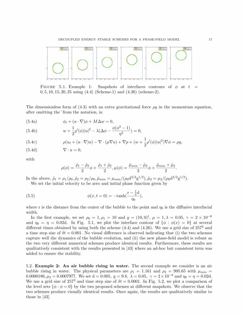
Figure 5.1. Example 1: Snapshots of interfaces contours of φ at t =0, 5, 10, 15, 20, 25 using (4.4) (Scheme-1) and (4.26) (scheme-2).

The dimensionless form of (4.3) with an extra gravitational force ρg in the momentum equation,after omitting the˜from the notation, is:

φt + (u · ∇)φ+M∆w = 0,(5.4a)

w +1

2ρ′(φ)|u|2 − λ(∆φ− φ(φ2 − 1)

η2) = 0,(5.4b)

ρ(ut + (u · ∇)u)−∇ · (µ∇u) +∇p+ (w +1

2ρ′(φ)|u|2)∇φ = ρg,(5.4c)

∇ · u = 0,(5.4d)

with

ρ(φ) =ρ1 − ρ2

2φ+

ρ1 + ρ2

2, µ(φ) =

µmin − µ2

2φ+

µmin + µ2

2.

In the above, ρ1 = ρ1/ρ0, ρ2 = ρ2/ρ0, µmin = µmin/(ρ0d3/2g1/2), µ2 = µ2/(ρ0d3/2g1/2).We set the initial velocity to be zero and initial phase function given by

φ(x, t = 0) = −tanh(r− 1

4d

η0),(5.5)

where r is the distance from the center of the bubble to the point and η0 is the diffusive interfacialwidth.

In the first example, we set ρ0 = 1, ρ1 = 10 and g = (10, 0)t, µ = 1, λ = 0.05, γ = 2 × 10−6

and η0 = η = 0.02d. In Fig. 5.1, we plot the interface contour of φ : φ(x) = 0 at severaldifferent times obtained by using both the scheme (4.4) and (4.26). We use a grid size of 2572 anda time step size of δt = 0.001. No visual difference is observed indicating that (i) the two schemescapture well the dynamics of the bubble evolution, and (ii) the new phase-field model is robust asthe two very different numerical schemes produce identical results. Furthermore, these results arequalitatively consistent with the results presented in [43] where an ad-hoc but consistent term wasadded to ensure the stability.

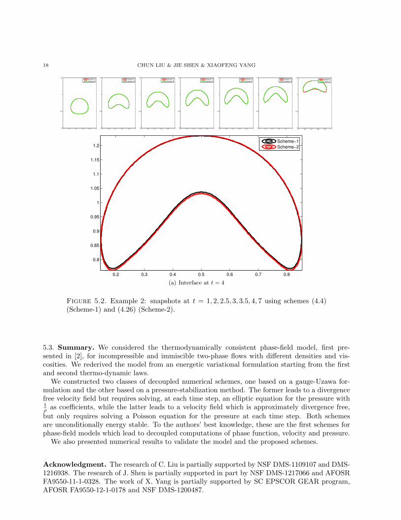
5.2. Example 2: An air bubble rising in water. The second example we consider is an airbubble rising in water. The physical parameters are ρ1 = 1.161 and ρ2 = 995.65 with µmin =0.0000186, µ2 = 0.0007977. We set d = 0.005, g = 9.8, λ = 0.05, γ = 2×10−8 and η0 = η = 0.02d.We use a grid size of 2572 and time step size of δt = 0.0001. In Fig. 5.2, we plot a comparison ofthe level sets φ : φ = 0 by the two proposed schemes at different snapshots. We observe that thetwo schemes produce visually identical results. Once again, the results are qualitatively similar tothose in [43].


0 0.2 0.4 0.6 0.8 10

0.5

1

1.5

Scheme−1

Scheme−2

0 0.2 0.4 0.6 0.8 10

0.5

1

1.5

Scheme−1

Scheme−2

0 0.2 0.4 0.6 0.8 10

0.5

1

1.5

Scheme−1

Scheme−2

0 0.2 0.4 0.6 0.8 10

0.5

1

1.5

Scheme−1

Scheme−2

0 0.2 0.4 0.6 0.8 10

0.5

1

1.5

Scheme−1

Scheme−2

0 0.2 0.4 0.6 0.8 10

0.5

1

1.5

Scheme−1

Scheme−2

0 0.2 0.4 0.6 0.8 10

0.5

1

1.5

scheme−1

scheme−2

0.2 0.3 0.4 0.5 0.6 0.7 0.8

0.8

0.85

0.9

0.95

1

1.05

1.1

1.15

1.2Scheme−1

Scheme−2

(a) Interface at t = 4

Figure 5.2. Example 2: snapshots at t = 1, 2, 2.5, 3, 3.5, 4, 7 using schemes (4.4)(Scheme-1) and (4.26) (Scheme-2).

5.3. Summary. We considered the thermodynamically consistent phase-field model, first pre-sented in [2], for incompressible and immiscible two-phase flows with different densities and vis-cosities. We rederived the model from an energetic variational formulation starting from the firstand second thermo-dynamic laws.

We constructed two classes of decoupled numerical schemes, one based on a gauge-Uzawa for-mulation and the other based on a pressure-stabilization method. The former leads to a divergencefree velocity field but requires solving, at each time step, an elliptic equation for the pressure with1ρ as coefficients, while the latter leads to a velocity field which is approximately divergence free,

but only requires solving a Poisson equation for the pressure at each time step. Both schemesare unconditionally energy stable. To the authors’ best knowledge, these are the first schemes forphase-field models which lead to decoupled computations of phase function, velocity and pressure.

We also presented numerical results to validate the model and the proposed schemes.

Acknowledgment. The research of C. Liu is partially supported by NSF DMS-1109107 and DMS-1216938. The research of J. Shen is partially supported in part by NSF DMS-1217066 and AFOSRFA9550-11-1-0328. The work of X. Yang is partially supported by SC EPSCOR GEAR program,AFOSR FA9550-12-1-0178 and NSF DMS-1200487.


References

[1] Helmut Abels. Existence of weak solutions for a diffuse interface model for viscous, incompressible fluids withgeneral densities. Comm. Math. Phys., 289(1):45–73, 2009.

[2] Helmut Abels, Harald Garcke, and Gunther Grun. Thermodynamically consistent diffuse interface models forincompressible two-phase flows with different densities. arXiv preprint arXiv:1011.0528, 2010.

[3] Helmut Abels, Harald Garcke, and Gunther Grun. Thermodynamically consistent, frame indifferent diffuseinterface models for incompressible two-phase flows with different densities. Mathematical Models and Methodsin Applied Sciences, 22(03), 2012.

[4] R. Abraham and J. E. Marsden. Foundations of mechanics. Benjamin/Cummings Publishing Co. Inc. AdvancedBook Program, Reading, Mass., 1978. Second edition, revised and enlarged, With the assistance of Tudor Ratiuand Richard Cushman.

[5] D. M. Anderson, G. B. McFadden, and A. A. Wheeler. Diffuse-interface methods in fluid mechanics. 30:139–165,1998.

[6] V. I. Arnold. Mathematical methods of classical mechanics. Springer-Verlag, New York, 1989. Translated fromthe 1974 Russian original by K. Vogtmann and A. Weinstein, Corrected reprint of the second (1989) edition.

[7] V. I. Arnold. Mathematical Methods of Classical Mechanics. Springer-Verlag, New York, 2nd ed. edition, 1997.[8] R. Becker, X. Feng, and A. Prohl. Finite element approximations of the Ericksen-Leslie model for nematic liquid

crystal flow. SIAM J. Numer. Anal., 46(4):1704–1731, 2008.[9] Franck Boyer. Nonhomogeneous Cahn-Hilliard fluids. Ann. Inst. H. Poincare Anal. Non Lineaire, 18(2):225–259,

2001.[10] J. W. Cahn and J. E. Hilliard. Free energy of a nonuniform system. I. interfacial free energy. J. Chem. Phys.,

28:258–267, 1958.[11] P. M. Chaikin and T. C. Lubensky. Principles of Condensed Matter Physics. Cambridge, 1995.[12] Feng Chen and Jie Shen. Efficient spectral-Galerkin methods for systems of coupled second-order equations and

their applications. J. Comput. Phys., 231(15):5016–5028, 2012.[13] W. Chen, S. Conde, C. Wang, X. Wang, and S. Wise. A linear energy stable scheme for a thin film model without

slope selection. Preprint, 2011.[14] H. Ding, P. D. M. Spelt, and C. Shu. Calculation of two-phase Navier-Stokes flows using phase-field modeling.

J. Comput. Phys., 226(2):2078–2095, 2007.[15] Weinan E and Jian-Guo Liu. Gauge method for viscous incompressible flows. Commun. Math. Sci., 1(2):317–332,

2003.[16] Yu. V. Egorov and M. A. Shubin. Foundations of the classical theory of partial differential equations. Springer-

Verlag, Berlin, 1998. Translated from the 1988 Russian original by R. Cooke, Reprint of the original Englishedition from the series Encyclopaedia of Mathematical Sciences [ıt Partial differential equations. I, EncyclopaediaMath. Sci., 30, Springer, Berlin, 1992; MR1141630 (93a:35004b)].

[17] David J. Eyre. Unconditionally gradient stable time marching the cahn- hilliard equation. In Computational andmathematical models of microstruc- tural evolution (San Francisco, CA, 1998),Mater. Res. Soc. Sympos. Proc.,Warrendale, PA, 529:39–46, 1998.

[18] X. Feng, Y. He, and C. Liu. Analysis of finite element approximations of a phase field model for two-phase fluids.Math. Comp., 76(258):539–571 (electronic), 2007.

[19] U. S. Fjordholm, S. Mishra, and E. Tadmor. Well-balanced and energy stable schemes for the shallow waterequations with discontinuous topography. J. Comput. Phys., 230:5587–5609, 2011.

[20] David Gilbarg and Neil S. Trudinger. Elliptic partial differential equations of second order. Classics in Mathe-matics. Springer-Verlag, Berlin, 2001. Reprint of the 1998 edition.

[21] J. L. Guermond, P. Minev, and J. Shen. An overview of projection methods for incompressible flows. Comput.Methods Appl. Mech. Engrg., 195:6011–6045, 2006.

[22] J.-L. Guermond and L. Quartapelle. A projection FEM for variable density incompressible flows. J. Comput.Phys., 165(1):167–188, 2000.

[23] J.-L. Guermond and A. Salgado. A splitting method for incompressible flows with variable density based on apressure Poisson equation. J. Comput. Phys., 228(8):2834–2846, 2009.

[24] M. E. Gurtin, D. Polignone, and J. Vi nals. Two-phase binary fluids and immiscible fluids described by an orderparameter. Math. Models Methods Appl. Sci., 6(6):815–831, 1996.

[25] Francis Hirsch and Gilles Lacombe. Elements of functional analysis, volume 192 of Graduate Texts in Mathe-matics. Springer-Verlag, New York, 1999. Translated from the 1997 French original by Silvio Levy.

[26] D. Jacqmin. Diffuse interface model for incompressible two-phase flows with large density ratios. J. Comput.Phys., 155(1):96–127, 2007.

[27] Junseok Kim. Phase-field models for multi-component fluid flows. Commun. Comput. Phys., 12(3):613–661, 2012.


[28] R. Kubo. The fluctuation-dissipation theorem. Reports on Progress in Physics, 1966.[29] P. Lin, C. Liu, and H. Zhang. An energy law preserving C0 finite element scheme for simulating the kinematic

effects in liquid crystal dynamics. J. Comput. Phys., 227(2):1411–1427, 2007.[30] C. Liu and J. Shen. A phase field model for the mixture of two incompressible fluids and its approximation by

a Fourier-spectral method. Physica D, 179(3-4):211–228, 2003.[31] J. Lowengrub and L. Truskinovsky. Quasi-incompressible Cahn-Hilliard fluids and topological transitions. R.

Soc. Lond. Proc. Ser. A Math. Phys. Eng. Sci., 454(1978):2617–2654, 1998.[32] R. Nochetto and J.-H. Pyo. The gauge-Uzawa finite element method part i: the navier-stokes equations. SIAM

J. Numer. Anal., 43:1043–1068, 2005.[33] L. Onsager. Reciprocal relations in irreversible processes. i. Physical Review, 37:405, 1931.[34] L. Onsager. Reciprocal relations in irreversible processes. ii. Physical Review, 38:2265, 1931.[35] A. Prohl. Projection and quasi-compressibility methods for solving the incompressible Navier-Stokes equations.

Advances in Numerical Mathematics. B. G. Teubner, Stuttgart, 1997.[36] J. Pyo and J. Shen. Gauge-uzawa methods for incompressible flows with variable density. J. Comput. Phys.,

221:181–197, 2007.[37] R. Rannacher. On Chorin’s projection method for the incompressible Navier-Stokes equations. Lecture Notes in

Mathematics, vol. 1530, 1991.[38] L. Rayleigh. Some general theorems relating to vibrations. Proceedings of the London Mathematical Society,

4:357–368, 1873.[39] L. Rayleigh. On the theory of surface forces ii. Phil. Mag., 33:209, 1892.[40] J. Shen. Efficient spectral-Galerkin method I. direct solvers for second- and fourth-order equations by using

Legendre polynomials. SIAM J. Sci. Comput., 15:1489–1505, 1994.[41] J. Shen. On error estimates of projection methods for the Navier-S tokes equations: second-order schemes. Math.

Comp, 65:1039–1065, July 1996.[42] J. Shen and X. Yang. An efficient moving mesh spectral method for the phase-field model of two-phase flows. J.

Comput. Phys., to appear, 2009.[43] J. Shen and X. Yang. Energy stable schemes for cahn-hilliard phase-field model of two-phase incompressible

flows. Chinese Ann. Math. series B, 31:743–758, 2010.[44] J. Shen and X. Yang. A phase-field model and its numerical approximation for two- phase incompressible flows

with different densities and viscositites. SIAM J. Sci. Comput., 32:1159–1179, 2010.[45] J. Shen and X. Yang. Decoupled, energy stable schemes for phase-field models of two-phase incompressible flows.

submitted, 2013.[46] Jie Shen. Modeling and numerical approximation of two-phase incompressible ows by a phase-eld approach. In

Multiscale Modeling and Analysis for Materials Simulation, Lecture Note Series, Vol. 9. IMS, National Universityof Singapore, 2011, Edited by W. Bao and Q. Du, pages 147–196.

[47] Jie Shen, Qi Wang, and Xiaofeng Yang. Mass-conserved phase field models for binary fluids. Comm. Comput.Phys., 2012, to appear.

[48] E. Tadmor and W. Zhong. Energy-preserving and stable approximations for the two- dimensional shallow waterequations. “Mathematics and Computation - A Contemporary View”, Proceedings of the third Abel Symposium,Springer, 3:67–94, 2008.

[49] J. van der Waals. The thermodynamic theory of capillarity under the hypothesis of a continuous density variation.J. Stat. Phys., 20:197–244, 1893.

[50] C. Wang and J.-G. Liu. Convergence of gauge method for incompressible flow. Mathematics of Computation,69:1385–1407, 2000.

[51] C. Wang and S. M. Wise. An energy stable and convergent finite-difference scheme for the modified phase fieldcrystal equation. SIAM J. Numer. Anal., 49:945–969, 2011.

[52] N. K. Yamaleev and M. H. Carpenter. A systematic methodology for constructing high-order energy stable wenoschemes. Journal of Computational Physics, 228(11):4248 – 4272, 2009.

[53] X. Yang, J. J. Feng, C. Liu, and J. Shen. Numerical simulations of jet pinching-off and drop formation using anenergetic variational phase-field method. J. Comput. Phys., 218:417–428, 2006.

[54] P. Yue, J. J. Feng, C. Liu, and J. Shen. A diffuse-interface method for simulating two-phase flows of complexfluids. J. Fluid Mech, 515:293–317, 2004.

decoupled energy stable schemes for a …shen/pub/lsy14.pdfof two-phase incompressible flows with...

Documents