1

Unified Computational Schemes for Incompressible and Weakly Compressible Flows

I. J. Keshtiban, F. Belblidia and M. F. Webster*

Institute of Non-Newtonian Fluid Mechanics, Department of Computer Science,

University of Wales, Swansea, SA2 8PP, UK.

* Author for correspondence. Email: m.f.webster@swansea.ac.uk

2

SUMMARY

A time-marching Taylor-Galerkin finite element algorithm, based on a pressure-correction

method with three fractional stages, is presented. The algorithm is applied in a consistent and

unified manner to weakly compressible and incompressible flows. For the compressible regime,

two types of density interpolation are investigated: a piecewise-constant form with gradient

recovery and a linear interpolation form. The background theory and consistency of the approach

are discussed. Numerical results are presented for high pressure-drop, 4:1 contraction flows,

under planar and axisymmetric frames of reference. Stability and accuracy of the method is

highlighted, bearing out the high quality of performance achieved for both compressible flow

density interpolation schemes, at low to vanishing Mach number. Primarily, we advocate the

piecewise-constant interpolation algorithm.

KEY WORDS: Finite element, Taylor-Galerkin, pressure-correction, compressible flow, zero Mach number.

3

1. INTRODUCTION

This paper presents a unified algorithmic framework to predict numerical solutions for flows that

range from incompressible to weakly compressible (at low Mach number). In this regard, we

commence from an existing software base dealing with incompressible flows, and incorporate

compressible considerations. This leads to a unified treatment for both incompressible and

weakly compressible flows. Initially, viscous Newtonian fluids are considered, for which recent

developments have advanced second-order accurate schemes (see Keshtiban et al. [1]). Briefly,

we provide some motivation for this study. In many flows, density may change with respect to

pressure, temperature and concentration. In fluid mechanics, Mach number characterise

compressibility effects conveying the ratio between fluid-speed and speed of sound ( cUMa = ).

For low Mach numbers (say less than 0.3), the flow regime may be considered as incompressible.

Beyond this regime at higher Mach numbers, compressibility effects should be taken into

account. At the singular limit of compressible flow, the equation system has time-scales of widely

varying magnitude, where sound waves travel at a much faster rate than those governing the

motion of the fluid. At low Mach number, Turkel [2] quotes the stiffness of the equation system

as being due to the large disparity between acoustic and convective time-scales.

Numerical computation at low Mach number poses a significant challenge. Yet, there are

several reasons to motivate the development of suitable methods to handle this regime. There are

many phenomena that occur at low Mach number, such as circulation in the oceans, bodily

functions of breathing and talking, free convection and combustion, recovery and exploration of

petroleum, liquid impact and jet cutting. Moreover, some flows contain both compressible and

incompressible regions, simultaneously. In such circumstances, some sections of the flow are

4

considered as incompressible with low Mach number, whilst other zones may prove somewhat

compressible. Second, it is preferable to work within a unified framework to handle wide ranges

of Mach number flow situations, including the incompressible limit (Ma0).

From a numerical standpoint, there are two principal methodologies commended to deal with

weakly compressible flows. One is to approach the problem based around compressible

algorithms. This leads to density-based schemes, which may be extended downwards in Mach

number to handle low Mach number situations. Alternatively, one may tackle the problem by

modifying incompressible algorithms, through say pressure-based schemes, leading outwards

from the Ma0 limit into the weakly compressible setting. With density-based methods, density

is the primary dependent variable extracted from the continuity equation, with pressure being

determined via an equation of state. With pressure-based methods, pressure is the primary

variable, so that density is the derived quality via the equation of state.

Density-based methods exhibit numerical shortcomings when dealing with low Mach number

flow situations (Ma<0.3). Under such setting, density variations are marginal and the continuity

equation effectively becomes decoupled from the momentum equation. Consequently, pressure

and density coupling is weakened. In addition, the relationship between velocity and pressure

may be defined via the divergence-free constraint on the velocity field. For high Mach number

regimes, pressure-density coupling is defined via an equation of state, with density given by the

continuity equation. However, Turkel [2] has recognized that, for the compressible flow equation

system, standard numerical schemes without modifications often fail to converge to the solution

of the incompressible equations, as the Mach number approaches zero. To extend density-based

schemes to deal with low Mach number situations and enhance solution convergence, two major

strategies have been proposed. The first appeals to preconditioning procedures, where the time

derivative of the governing equations is premultiplied by a suitable (preconditioning) matrix. This

5

scales the eigenvalues of the system to within similar order. A comprehensive review of

preconditioning methods may be found in Turkel [3]. The second strategy follows asymptotic

procedures, leading to a perturbed form of equations. Here, specific terms are discarded, so that

the physical acoustic waves are replaced by pseudo-acoustic modes [4].

Alternatively, pressure-based schemes represent extensions to pressure-correction or

projection methods [5] for incompressible flows. Projection methods were pioneered by Chorin

[6] and Temam [7]. These are a fractional-staged formulations, which decouple velocity and

pressure terms from the momentum equations, leading to an auxiliary Poisson equation for

pressure on each time-step (see Townsend and Webster [8] and Hawken et al. [9]). Such a

fractional-staged formulation is designed to significantly reduce computational overheads in

transient incompressible viscous flow computations, when using primitive variables [10].

Normally, projection methods are based on three distinguish stages over each time-step. First, the

momentum equation is employed to obtain an approximation of velocity. Second, pressure is

obtained as the solution to a Poisson equation. Third, velocity is corrected at a final stage. In

addition, projection methods have been employed within a finite volume context, through the

SIMPLE (Semi-Implicit-Pressure-Linked-Equation) family of methods, as first introduced by

Patankar [11] for incompressible flows. The extension of such pressure-based methods towards

compressible flows was proposed by Patankar [12], and later adapted by Isaa [13], Rhie [14],

Karki [15] and Mc-Gurik [16].

Donea [10] introduced a fractional-step formulation within a finite element context of

pressure-correction form. In addition, there is synergy between pressure-correction/fractional-

staged schemes and so-called Taylor-Galerkin schemes [17] for convection problems. This is due

to their common semi-discrete design philosophy, temporal preceding spatial discretization. The

ideology behind the Taylor-Galerkin methodology is to generate high-order accurate time-

6

stepping schemes, taking advantage of the high spatial resolution attainable, say via Galerkin

approximation. Taylor-Galerkin methods may be posed in various guises (of implicitness) and

normally incorporate Lax-Wendroff representation [18], within Taylor series expansions in time

to develop improved time-stepping schemes. Based on proposals of Van Kan [19], this was

recognised by Townsend and Webster in the viscoelastic context [8], who developed a finite

element Taylor-Galerkin/Pressure-Correction (TGPC) hybrid scheme to attain second-order

accuracy.

Having briefly reviewed density-based and pressure-based procedures applied to compressible

and incompressible flows, we turn attention to the development of a unified framework, to tackle

both flow scenarios. The specific nature of the flow equations is the starting point in developing

such a framework. One observes that these equations switch in type depending on flow setting.

For example, the equations for viscous compressible flow form a hyperbolic-parabolic system

with finite wave-speed, whilst those for incompressible flow assume an elliptic-parabolic system

with infinite propagation rates. Moreover, depending on local Mach number, in some regions

flow type is elliptic-dominant, whilst in other sections is hyperbolic-dominant. A unified

algorithm should reflect the capability to accommodate for such switch in type (on a local Mach

number basis). Based on this philosophy and under finite element considerations, Mittal [19]

developed a unified density-based algorithm. In this scheme, the governing equation for pressure

was selected based on local Mach number. In the incompressible limit, pressure was derived from

the divergence-free constraint. Alternatively, the equation of state governs the solution for

pressure in compressible flows. In the present study, we have found that pressure-based methods

are more attractive, circumventing the need to derive density as an intermediate variable and to

extract pressure.

7

A well known and successful unified approach to simulate incompressible, as well as

compressible regimes, was introduced by Zienkiewicz and co-workers. Here, a series of articles

[21-23] have appeared on the characteristic-based-split procedure (CBS), employed in the context

of finite element pressure-correction schemes. The process is practically identical to the TGPC

scheme, noting the essential difference that pressure gradient terms are omitted in the momentum

equation. Instead with the CBS-scheme, the pressure is employed as a source term at a third

fractional-equation stage. This separation of variables/equations (velocity from pressure) gives

rise to a number of positive attributes. One such, is that the Babuska-Bezzi stability restriction,

from the original Taylor-Galerkin procedure, no longer applies [20,21]. Hence, equal order and

convenient pressure-velocity interpolants are permitted†. One issue remains with the CBS-

scheme, that of imposition of boundary conditions for any given problem. This issue is somewhat

controversial in the application of fractional-staged schemes. In the CBS-scheme, boundary

conditions are not explicitly imposed upon the velocity field at the first fractional-equation stage.

Hence, velocity must be computed on the domain boundary. For viscous flow, for instance, this

leads to the computation of boundary integrals [21], which begs questions of discrete

representation. Boundary conditions upon pressure are imposed within the second fractional-

equation stage (representing continuity satisfaction). Noticeably, the CBS procedure has been

assessed across a number of different flow settings and found to perform satisfactorily. For

example, on transonic and supersonic flows, low Mach number flows with low and high

viscosity, and in addition, shallow-water wave flow problems.

† Within a viscous context, and particularly so in the viscoelastic regime, parabolic velocity profiles demand quadratic level interpolation in field representation for accuracy. This negates the need to lower the level of velocity interpolation, as secondary gradient field representation becomes all important.

8

In a recent article [1], an extension of an incompressible TGPC scheme has been proposed for

weakly compressible flows. There, stability and accuracy of both incompressible and weakly

steady compressible flows have been highlighted on some benchmark problems. The concern

behind the present study is to capture high quality of performance for compressible flow

algorithms, at low to vanishing Mach number. In this fashion, a unified scheme is constructed

around existing incompressible algorithms and associated software. The base formulation-

framework proposed (TGPC), may be viewed as a pressure-correction scheme split into three

distinct, fractional-stages. At a first stage (doublet equation-set), the momentum equation is

utilised to predict the velocity field at a half-stage. Subsequently, the momentum equation is

employed to compute the velocity at a full-step (Lax-Wendroff style, two-step Taylor-Galerkin

phase). The second stage solves for temporal difference in pressure on the time step (conveying

second-order to the scheme and some additional attractive boundary condition options [19]). The

third stage completes the time-step loop for velocity correction, utilising the non-solenoidal

velocity field intermediate variable generated. In contrast with the CBS technique, in our TGPC

approach, pressure gradients are not omitted from the momentum equation, so that, physical

boundary conditions are applied in a conventional manner (i.e. via tractions). In both fractional-

staged schemes (TGPC and CBS) and by construction, the equations are able to accommodate

switch of equation-type depending on local Mach number. In our TGPC unified implementation

for compressible flow, we represent density variation through pressure via a suitably extended,

well-established Tait equation of state [24]. Two types of finite element interpolation of density

are employed to handle the weakly compressible regime: a piecewise-constant form

(incompressible per element), with recovery for density gradients (during the second-stage); and

a linear interpolation form. We have demonstrated in our earlier studies that these key

9

modifications do not degrade second-order accuracy of the original incompressible TGPC

scheme.

The present paper is organized as follows: the governing equations for compressible viscous

flows are expounded in Section 2. In Section 3, we introduce the equation stages for the Taylor-

Galerkin/pressure-correction scheme, followed by the finite element (FE) discretization adopted.

In Section 4, the method is applied and a sample of results is presented for a benchmark test-

problem. Here, we consider planar and circular 4:1 contraction flow under isothermal viscous

conditions. The schemes proposed are validated for consistency in terms of mesh refinement.

Comparison between incompressible and compressible regimes for vanishing Mach number are

conducted, highlighting the attractive properties of this proposed unified scheme.

2. GOVERNING EQUATIONS

For a compressible viscous flow under isothermal conditions, governing equations for transport

of momentum and mass conservation may be expressed in dimensionless form, viz

]..[ PUURt

Ue ∇−∇−∇=

∂∂ ρτρ (1)

( ) 0=∇+∂∂

U.Rt e ρρ

(2)

where ρ , U , τ , P represent dimensionless dependent variables of density, velocity, stress and

pressure. Dimensionless independent variables are t and x, representations of time and space,

respectively. The dimensionless group Reynolds number is defined as:

o o

e

U LR

ρµ

= . (3)

10

Such dimensionless form is obtained by introducing characteristic scales on density 0ρ , viscosity

µ , length L (exit half-channel width), and velocity U0 (exit flow, average velocity). Note, for

incompressible flow with constant density, the continuity equation reduces to: 0=∇ U. .

For compressible flow, a third equation relating density to pressure is required. In the case of

liquids, the modified Tait [24] equation of state is adopted of the form:

m

BP

BP

=

++

00 ρρ

(4)

where, m and B are scalar parameters and oP , oρ denote reference scales for pressure and

density, respectively. Note, in a strict sense, Eq.(4) is exact only for isentropic change.

Nevertheless, it may be applied to reasonable precision in the general case, since m is

independent of entropy, and B and oρ are constants [25]. In the present analysis, the energy

equation has been discarded, as we are interested in low Reynolds number isothermal flows,

where kinetic considerations are negligible.

After rearranging and differentiating the equation of state, we gather:

( ) 2),(

0

01 )(tXm

m cBPmBP

mP =+=

+=

∂∂ −

ρρρ

ρ (5)

where ),( tXc represents the speed of sound.

To address spatial discretisation, a finite element representation is applied, as outlined below.

11

3. TAYLOR-GALERKIN/PRESSURE-CORRECTION SCHEME

AND FE DISCRETIZATION

In order to outline the TGPC-scheme, we first indicate the constructive steps to follow in the

incompressible context. Then, it is a straightforward matter to provide the necessary steps to

adjust to the compressible TGPC-version. To begin, we may consider the semi-discrete

incompressible equation system,

( ) nnn

e

nn

PPUURt

UU ∇−−∇−∇−∇=∆

− +++

θθρτρα

1]..[ 121

(6a)

.0. 1 =∇ +nU (6b)

We observe that ( 0,0 == θα ) yields an explicit-form momentum equation (first-order).

Alternatively, ( 21,1 == θα ) provides Crank-Nicolson pressure-gradient discretisation and the

need for a half-step solution in ( ) 2

1

, +nUτ . This is now of second-order form (see Van Kan [19]).

The term at level 2

1+n

t may be evaluated through a the two-step predictor-corrector structure, as in

Taylor-Galerkin schemes. The pressure gradient terms may be regrouped as,

[ ] nnn PPP ∇−∇−∇− +1θ (7)

and handled via splitting of terms across pressure-correction stages. Retaining only nP∇ within

the first stage and utilizing the two-step doublet realises,

stage 1a

nne

nn

PUURt

UU ∇−∇−∇=∆

−+

]..[2/

2

1

ρτρ (8)

12

stage 1b

nn

e

n

PUURt

UU ∇−∇−∇=∆− +

2

1

]..[* ρτρ . (9)

In Eq.(9) we have introduced U* as an auxiliary free-variable, a non-solenoidal velocity

variable, utilised to extract the omitted difference term on pressure gradient, and to realise a third

fractional-stage equation

( )nnn

PPt

UU −∇−=∆

− +∗+

11

θρ . (10)

Here, Un+1 satisfies Eq.(6b). By taking the divergence of Eq.(10), one takes advantage of

Eq.(6b) and forms the second-stage Poisson equation for pressure, as

( ) ( )*12 . UPPt nn ρθ −∇=−∇∆ + . (11)

In summary, when applying the TGPC-scheme to the governing equations for viscous

incompressible flows, three fractional-staged equations emerge. In stage 1a –Eq.(8)-, a half time-

step velocity field at (n+1/2) is predicted, based on the previous time-step (n) information

(prediction stage). This is followed by a full-step correction at stage 1b –Eq.(9)- to calculate the

auxiliary free variable U*. This is utilised in stage 2 –eq(11)- through a Poisson equation, to

determine pressure-difference over the full time-step, (n) to (n+1). At stage 3 –Eq.(10)-, the

incompressible end-of-loop velocity field is extracted, based on the pressure-difference and the

non-divergence-free velocity (final correction stage). The TGPC-scheme consists of Eq.(8), (9),

(11) and (10), in that order on each time-step.

Note, that the momentum equations for compressible and incompressible flows are identical

(bar variation in density), whilst differences emerge due to the various alternative forms of the

continuity equation. The compressible continuity equation, semi-discretised in time assumes the

form

13

( ) 0. 11

=∇+∆− +

+nn

e

nn

URt

ρρρ. (12)

To extend the incompressible TGPC-version into the compressible context, only modification

at stage 2 is necessary. Oncemore, appealing to Eq.(10) and taking the divergence operation, we

gather

( ) ( )nnn PPtUU −∇∆−=−⋅∇ ++ 12*1 θρρ , (13)

which may be introduced within Eq.(12) to provide

).()( *121

1 UPPtt

R nnnnn

e ρθρρ −∇=−∇∆−∆

− ++

− . (14)

To progress further for compressible flow, it is necessary to switch reference from density to

that of pressure. In order to accomplish this, we employ the chain rule on the derived form of the

Tait equation of state in Eq.(5), gathering

t

P

ct tX ∂∂=

∂∂

2),(

1ρ. (15)

Finally, after semi-discretising in time, we substitute Eq.(15) into Eq.(14) to realise a modified

temporal evolutionary expression for pressure. This form may be employed at stage 2 replacing

Eq.(11), in the context of compressible flows. The corresponding equation now becomes:

Stage 2:

).()(1 *12

1

2),(

UPPtt

PP

cRnnn

nn

tXe

ρθ −∇=−∇∆−∆

− ++

. (16)

Note, Eq.(16) adopts an important role in the development of the compressible flow algorithm.

It displays some interesting features: the first term on the left-hand-side is a first-order time

derivative representation, whilst the second term is governed by a Laplacian operator (elliptic

properties). In addition, on the right-hand-side, density is a direct function of pressure (to be

14

interpreted via the equation of state). When the flow is incompressible, speed of sound

asymptotes to infinity. In this context, the first term as the right-hand-side vanishes and elliptic

character dominates in Eq.(16). Alternatively, for compressible flows, depending upon the Mach

number level (local compressibility), the balance of type-domination within the equation adjusts

between elliptic and hyperbolic.

A FE Galerkin spatial discretization is adopted, leading to approximations of primary variables

( ),U x t and ( ),P x t in the velocity and pressure fields, respectively. These are taken over

triangular elements of reference, as follows:

)()(),( xtUtxU jj φ= , j=1,6 and )()(),( xtPtxP kk ψ= , k=1,3, (17)

where interpolant notation implies, ( )xφ , as continuous quadratic and, ( )xψ , as piecewise linear

on the triangular elements. Time-dependent velocity and pressure nodal-vectors are represented

as U and P, respectively. Depending on the treatment of diffusion terms (in the momentum

equation), the scheme may be developed in explicit form (=0), where care must be taken in

choosing appropriate size of time-step, or include some implicitness, by say semi-implicit Crank-

Nicolson representation (=1/2). The treatment of diffusion terms may be represented via:

nnnn

τττταα

.2

... 2 ∇+∇−∇=∇

++. (18)

To enhance stability of the scheme, the semi-implicit scheme is adopted and the discretized

equation for compressible TGPC stages may be expressed in fully-discrete matrix form as:

15

Stage 1a:

[ ]nTU

n

U PLUUNUSUSt

M−+−=

∆

+

∆+

)(2

1

2/2

1

ρρ (19)

Stage 1b:

( ) [ ] [ ] 2

1* )(

2

1 +−−−=∆

+

∆nnT

UU UUNPLUSUSt

Mρ

ρ (20)

Stage 2:

( ) *11 ULPKtt

MR nC

eρθ −=∆

∆+

∆+− (21)

Stage 3:

( ) 1*11 ++ ∆=−∆

nTn PLUUMt

θρ (22)

where, in the case of planar coordinates, matrix notation implies:

( ) Ω= Ω

dM jiijφφρρ (23)

( ) Ω

Ω∇⋅= dUN jiij)( φρφρ (24)

( ) Ω∇⋅∇= Ω

dK jiij ψψ (25)

( ) ( ) Ω⋅∇= Ω

dLkjiijk φψ (26)

( ) ( ) 2,1,, == mlSS ijlmijU (27)

( ) Ω

∂∂

⋅∂∂−

∂∂

⋅∂∂+

∂∂

⋅∂∂=

Ω

dxxyyxx

S jijijiij

φφφφφφµ32

211 (28)

( ) Ω∂

∂⋅

∂∂

= Ω

dxy

S jiij

φφµ12 (29)

16

( ) Ω

∂∂

⋅∂∂

−∂

∂⋅

∂∂

+∂

∂⋅

∂∂

= Ω

dyyyyxx

S jijijiij

φφφφφφµ3

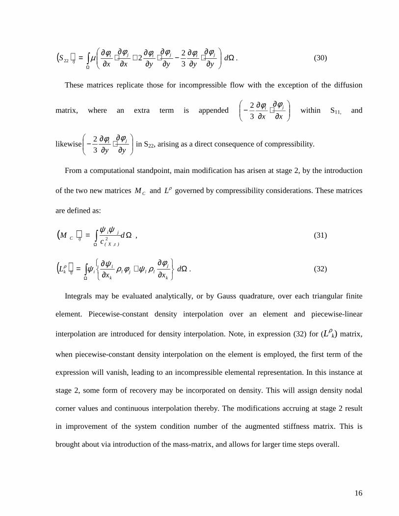
2222 . (30)

These matrices replicate those for incompressible flow with the exception of the diffusion

matrix, where an extra term is appended

∂∂

⋅∂∂

−xx

jiφφ

3

2 within S11, and

likewise

∂∂

⋅∂∂

−yy

jiφφ

3

2 in S22, arising as a direct consequence of compressibility.

From a computational standpoint, main modification has arisen at stage 2, by the introduction

of the two new matrices CM and ρL governed by compressibility considerations. These matrices

are defined as:

( ) Ω= Ω

dc

M)t,X(

jiijC 2

ψψ, (31)

( ) Ω

∂∂

+∂∂

= Ω

dxx

Lk

jlljl

k

liijk

φρψφρψψρ . (32)

Integrals may be evaluated analytically, or by Gauss quadrature, over each triangular finite

element. Piecewise-constant density interpolation over an element and piecewise-linear

interpolation are introduced for density interpolation. Note, in expression (32) for (Lρk) matrix,

when piecewise-constant density interpolation on the element is employed, the first term of the

expression will vanish, leading to an incompressible elemental representation. In this instance at

stage 2, some form of recovery may be incorporated on density. This will assign density nodal

corner values and continuous interpolation thereby. The modifications accruing at stage 2 result

in improvement of the system condition number of the augmented stiffness matrix. This is

brought about via introduction of the mass-matrix, and allows for larger time steps overall.

17

The difference between the CBS procedures and our implementation lies mainly in the

treatment of pressure terms. With the CBS-scheme, the pressure-gradient term is discarded from

stage 1, and evaluated by design at stage 3, where it is treated as a source correction-term. The

imposition of consistent boundary conditions introduces complications. In the application of

fractional-step methods, this issue is somewhat controversial. In our implementation, the issue is

circumvented through the freedom of choice of the auxiliary variable U*. One can choose

1+∗ = nUU on the domain boundary, which simplifies the treatment of boundary conditions for the

pressure-difference 1+∆ nP of stage 2. Hence, in steady flow situations, homogeneous Newman

conditions are imposed on temporal pressure-difference (and not pressure itself) at stage 2.

Finally, both CBS and TGPC-schemes demonstrate the ability to accommodate for switch-of-

equation type, according to localised Mach number levels encountered at stage 2 (see Eq.(16)). In

addition, an iterative preconditioned Jacobi solver is adequate to compute each fractional-stage.

That is, with exception of the temporal pressure-difference equation (stage 2), which is solved

through a direct Choleski procedure.

4. NUMERICAL EXAMPLES

For isothermal viscous flows, a contraction flow problem is employed to quantify the behaviour

of these unified schemes within low Mach number regimes. The total length of the channel is

76.5 units and the contraction ratio is 4:1. Both planar and axisymmetric geometric settings are

considered (see Figure 1). No-slip boundary conditions are assumed on solid boundaries. At

flow-entry, we consider a parabolic flow profile for longitudinal velocity, with its maximum set

to unity; the cross-sectional component vanishes. At the outlet, a natural condition is adopted on

18

longitudinal velocity and the cross-sectional component again vanishes. At the outlet, a pressure

reference is set to zero. Note, only the half-geometry of the channel is employed in these

simulations taking advantage of problem symmetry. Reynolds number (Re) is set to unity. There

are two variant of the unified scheme depending on the density implementation employed

(constant within the finite element, with recovery of the gradients, or linear). Our strategy in the

present study has been to adjust the values of the Tait parameter pairing (m, B), to alter the type

of flow under consideration.

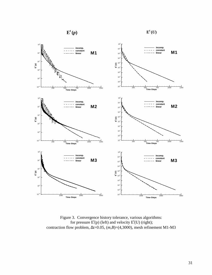
First, the unified framework is assessed with respect to time-stepping convergence history and

spatial accuracy properties. For this purpose, a multi-block meshing strategy is employed to

discretized the half-contraction channel-geometry, with conformal mapping in each sub-block

and matching of boundary nodes at interfaces. Three different meshes M1, M2 and M3 with

different levels of refinement are employed. The meshes are illustrated in Figure 2 and their

characteristics are quantified in Table I∗. We have need to define a temporal relative-increment

L2-norm to govern time-stepping convergence history (history tolerance) as:

1

1

)(+

+ −=

n

nn

t

X

XXXE . Results for convergence history tolerance on pressure (Et(p)) and

velocity (Et(U)) are displayed in Figure 3. This covers three different meshes and algorithmic

variants. The Tait parameters are set to (m,B)=(4,3000). As one suppresses error in the velocity

field through mesh refinement, one also controls the oscillatory evolutionary patterns for error-

history in pressure. This is anticipated, since convergence in pressure is constrained in a

Lyapunov norm, see Van Kan [19].

∗ Details are recorded for total numbers of elements, nodes, degree of freedom, corner mesh density and minimum element size (see Matallah et al. [26] and Baloch et al. [27]).

19

Figure 4 illustrates pressure and stream function fields, with their associated contour levels,

for the three meshes. In this figure only piecewise-constant density interpolation results are

illustrated (see below). In Table II, values of pressure and vortex information are given at the

contraction (sample location highlighted by a cross ‘+’ in Figure 1). Table III illustrates values

for velocity (Ux, Uy) at the same location. Note that from Tables II and III, for the same

compressibility setting, the piecewise-constant and the linear density interpolations deliver

similar results for a particular mesh size. The associated contour plots are smoother on finer

meshes. Note, that mesh M2 is felt adequate for detailed coverage below. In addition, mesh M2

was able to highlight the salient corner vortex and is less computationally expensive compared to

the finest mesh M3.

4.1. Planar contraction flow

This example is introduced to demonstrate algorithmic consistency in representing behaviour for

a high pressure-drop situation, which reflects excessive compressibility effects. All simulations

are based on mesh M2 (Figure 5a). The first two sets of figures present the adjustment of

different variables (velocity, pressure, density and Mach number) for piecewise-constant (Figure

6) and linear density interpolations (Figure 7) around the contraction zone. A highly compressible

flow situation is considered through (m,B)=(2,300). To present the results, sampled spatial

locations are selected and shown in Figure 5b. Numerical solutions are presented at these

sampled spatial locations for the two cases to demonstrate the difference in the results. As

presented in Table IV on sampled locations, similar variable contour patterns (at equitable levels)

are observed for both compressible representations around the contraction. In Mach number,

contour field plots reflect some differences, according to the choice of density interpolation

20

employed. This is because the Mach number is related to speed of sound, which itself is linked

directly to density, via the Tait equation. Hence, the level of density interpolation comes into

play. Therefore, under piecewise-constant density interpolation, Mach number contours are non-

smooth over elements of large size (see Figure 5a).

Next, a comparison of both density interpolation schemes is conducted with (m,B)=(4,300).

Figure 8 presents solution profiles for different variables at the contraction channel centreline for

both schemes. The results provide clear evidence that low-order density interpolation with

gradient recovery, is able to reproduce results comparable to those with linear density

interpolation. Near the exit, a discrepancy of about ten percent is observed in Mach number, with

those for constant density interpolation being higher than those for the linear interpolation

alternative. This departure is due mainly to the adjustment in both velocity and pressure across

the exit zone, and to some degree to the mesh quality there (see Figure 5a).

Finally, the ability of the compressible algorithm to deal with a wide range of low Mach

number (0<Ma<0.3) is highlighted. Figure 9 presents trends in solution profiles for different

variables at the contraction channel centreline, based on variation in compressibility settings,

adjusting Tait parameters accordingly. These trends reflect adjustment from the incompressible

towards the mildly compressible setting. In the compressible regime, only piecewise-constant

density interpolation has been employed, as both constant and linear representations lead to

practically identical results. Centreline solution profiles indicate that the compressibility setting

has little affect on the velocity field before the contraction. As the flow becomes more

compressible, some affect is visible beyond this zone once the liquid accelerates. At flow-entry,

pressure and density are larger for compressible flow. This highlights how much

‘compressibility’ impacts upon the flow kinematics.

21

4.2. Axisymmetric contraction flow

The previous example is reconsidered, but under an axisymmetrical frame of reference. In this

case, pressure-differences exceed those for the Cartesian equivalent. A principal goal here is to

demonstrate the ability of these compressible implementations to deal with incompressible flows

(Ma0). Hence, to demonstrate effective use of compressible algorithmic implementations to

simulate weakly compressible, as well as incompressible flows, through a unified schema. To the

same end, stability characteristics of the algorithm are quantified under different compressibility

parameters settings.

First, as above for planar flow, we confirm that similar trends are observed in field variables

based on both compressible algorithmic variants (see figures 6 and 7). In Figure 10, solution

profiles are presented for different variables at the contraction channel centreline for both forms

of density interpolation. Tait parameters are set to (m,B)=(5,3000), leading to mild

compressibility influences. Again, for this case, the results demonstrate that low-order density

interpolation with gradient recovery is comparable to that for linear interpolation.

In Figure 11, trends in solution profiles for different variables at the contraction channel

centreline are provided. Tait parameters are set, varying from those for incompressible towards

mildly compressible conditions. For the compressible regime, only piecewise-constant density

interpolation results are displayed. Similar solution trends are observed when compared to

Cartesian results.

After outlining the overall behaviour of the three algorithmic implementations

(incompressible, piecewise-constant and linear density interpolation) within a unified framework,

we turn attention to algorithmic stability. In particular, we conduct a parameter sensitivity

22

analysis to assess variation with the compressibility parameter set (m,B). Here, based on

piecewise-constant density interpolation, convergence history tolerances for pressure (Et(p)) and

velocity (Et(U)) are adopted to characterise stability. In Figure 12, plots of pressure and velocity

convergence history tolerances are presented, based on various Tait parameters settings. Note that

large values in the Tait parameter pairing are set for incompressible flow. For the three plots to

the left, the m-parameter is held constant (m=10), whilst the B-parameter varies from 105

(incompressible, top plot) down to 103 (compressible, bottom plot). For the three plots to the

right, the B-parameter is held constant (B=104), and m varies from 103 (incompressible, top plot)

down to 5 (compressible, bottom plot). The plots highlight the fact that the compressible

algorithm is more stable, in particular within the incompressible flow regime setting. Stability for

pressure is more difficult to assess when compared to velocity, due to the physics of the flow and

to the fractional-staged procedure (second stage). Nevertheless by design, the present approach

will ultimately fail to simulate highly compressible flow, as this would necessitate consideration

of the kinetic equation (which is neglected here).

Finally, the challenging issue of the present study is considered: addressing the effectiveness

of the unified scheme to deal with very low Mach number situations. For this, the Tait parameters

are elevated to high levels (m=102 or 103 and B=105), and one observes improvement in stability

and convergence-rate of the compressible implementations. That is, in comparison to the

convergence of the incompressible flow algorithm, as illustrated in Figure 13. This is attributed to

improvement in system condition number, via inclusion of the stage 2 mass-matrix, permitting

the use of larger time steps. Results for this particular case are tabulated in Table IV. The data

highlight the match in sample solution values between incompressible and compressible (with Ma

0) algorithmic implementations, in all variables and over different zones for the contraction

23

flow benchmark. By setting high-level Tait parameter pairings, a zero Mach number limit may be

approached. Once again, results demonstrate that, in the zero Mach number limiting regime,

piecewise-constant density interpolation, with recovery of gradients during the second stage, is

equitable to linear density interpolation. Based on these findings, we have established that the

compressible algorithmic implementations may be employed effectively to simulate weakly

compressible, as well as incompressible flow scenarios. Hence, we have established the required

unified framework, the object of the present study.

5. CONCLUSION

Two algorithmic implementations have been investigated to simulate weakly compressible liquid

flows, within a triangular-based finite element representation. The first employs a piecewise-

constant density interpolation with recovery to compute density-gradients. The second algorithm

utilises linear interpolation for density. These algorithmic variants have been implemented within

the context of a fractional-staged, Taylor-Galerkin approximation within a pressure-correction

scheme.

A high pressure-drop, 4:1 contraction flow, under planar and axisymmetric setting, has been

employed to analyse consistency and accuracy of both implementations. Both forms perform in a

similar fashion, leading to comparable levels of accuracy. The convergence-rate of both

algorithms has improved over that for the incompressible implementation. This is attributed to

improvement in system condition number via mass-matrix inclusion at the second-stage, thus

allowing for larger time-steps overall.

24

These compressible algorithmic variants have been shown capable of simulating flow with

low to zero Mach number (incompressible regime). Based on these compressible algorithmic

implementations, a zero Mach number limit has been reached by adjusting Tait parameter

parings. In this manner, compressibility effects within the liquid flow are controlled, to approach

the incompressible limit. Under such circumstances, results match well those for the compressible

algorithm and those for the ‘purely’ incompressible algorithm. These findings allow the user to

apply the compressible algorithm in a unified manner for both compressible and incompressible

regimes.

The proposed compressible algorithms have been implemented effectively within an

incompressible software-base. This is made straightforward with piecewise-constant density

interpolation, using recovery for density-gradients and density scaling for elemental matrices.

Finally, the piecewise-constant density interpolation option is preferred to the linear density

counterpart. They both perform equally, displaying similar properties of accuracy and stability,

yet the piecewise-constant option is the more efficient in implementation.

ACKNOWLEDGEMENTS

The financial support of EPSRC grant GR/R46885/01 is gratefully acknowledged.

25

REFERENCES

1. Keshtiban IJ, Belblidia F and Webster MF. Second-order schemes for weakly steady

compressible liquid flows. submitted to J. Comput. Physics. 2003.

2. Turkel E. Preconditioned methods for solving the incompressible and low speed

compressible equations. J. Comput. Physics. 1987; 72: 277-298.

3. Turkel E. Review of preconditioning methods for fluid dynamics, Technical Report 92-47,

Institute for computer applications in science and engineering, NASA Langley Research

center, September 1992.

4. Choi YH, Merkle CL. The application of preconditioning in viscous flows. J. Comput.

Physics. 1993; 105: 207-223.

5. Peyret R, Taylor TD. Computational Methods for Fluid Flow, Springer-Verlag, New York,

1983.

6. Chorin AJ. Numerical solution of the Navier-stokes equations. Math. Comp. 1968; 22: 745-

762.

7. Temam R. Sur l’approximation de la solution de Navier-Stokes par la méthode des pas

fractionnaires. Archiv. Ration. Mech. Anal. 1969; 32: 377-387.

8. Townsend P and Webster MF. An algorithm for the three-dimensional transient simulation

of non-Newtonian fluid flows, in Transient/Dynamic Analysis and Constitutive Laws for

Engineering Materials, Int. Conf. Numerical Methods in Engineering: Theory and

Applications - NUMETA 87", eds. G.N. Pande and J. Middleton, Nijhoff, Kluwer,

Dordrecht, 1987; vol 2: T12/1-11.

26

9. Hawken DM, Tamaddon-Jahromi HR, Townsend P and Webster MF. A Taylor-Galerkin

based algorithm for viscous incompressible flow. Int. J. Num. Meth. Fluids. 1990; 10:

327-351.

10. Donea J, Giuliani S, Laval H, and Quartapelle L. Finite element solution of the unsteady

Navier-Stokes equations by fractional step method. Meth. Appl. Mech. Engng. 1982; 30:

53-73.

11. Patankar SV and Spalding DB. Heat and Mass Transfer in Boundary Layer, 2nd edition,

Morgan-Grampian, London, 1970.

12. Patankar SV. Calculation of unsteady compressible flows involving shocks. Report

UF/TN/A/4, Imperial College, 1971.

13. Isaa RI, Lockwood FC. On the prediction of two-dimensional supersonic viscous

interactions near walls. AIAA Journal. 1977; 15: 182-188.

14. Rhie CM, Stowers ST. Navier-Stokes analysis for high-speed flows using a pressure

correction algorithm. AIAA Paper: 87-1980, 987.

15. Karki KC and Patankar SV. Pressure-based calculation procedure for viscous flows at all

speeds in arbitrary configurations. AIAA Journal.1989; 27 (9) :1167-1174.

16. Mc-Gurik JJ, and Page GJ. Shock-capturing using a pressure correction method. AIAA

Journal. 1989; 28 (10): 1751-1757

17. Donea J. A Taylor-Galerkin method for convective transport problems. Int. J. Numer.

Meth. Engng. 1984; 20: 101-120.

18. Lax P and Wendroff B. Systems of conservation laws. Comm. Pure Applied Math. 1960;

XII I : 217-237.

19. Van Kan J. A second-order accurate pressure-correction scheme for viscous

incompressible flow. SIAM J. Sci. Stat. Compt. 1986; 7: 870-891.

27

20. Mittal S, Tezduyar TE. A unified finite element formulation for compressible and

incompressible flows using augmented conservation variables. Computer Methods in

Applied Mechanics and Engineering. 1998; 161: 229-243.

21. Zienkiewicz OC, Condina R. A general algorithm for compressible and incompressible

flow - Part I: The split characteristic-based scheme. Int. J. Num. Meth. Fluids. 1995; 20:

869-885.

22. Zienkiewicz OC, Morgan K, Sataya Sal BVK, Codina R and Vasquez M. A general

algorithm for compressible and incompressible flow - Part II: Test on the explicit form.

Int. J. Num. Meth. Fluids. 1995; 20: 887-913.

23. Zienkiewicz OC, Nithiarasu P, Codina R, Vazquez M and Ortiz P. The characteristic-

based-split procedure: An efficient and accurate algorithm for fluid problems. Int. J. Num.

Meth. Fluids. 1999; 31: 359-392.

24. Tait PG, HMSO, London, 1888; 2(4).

25. Brujan EA. A first-order model for bubble dynamics in a compressible viscoelastic liquid.

J. Non-Newt. Fluid Mech. 1999; 84: 83-103.

26. Matallah H, Townsend P and Webster MF. Recovery and stress-splitting schemes for

viscoelastic flows. J. Non-Newt. Fluid Mech. 1998; 75: 139-166.

27. Baloch A, Townsend P and Webster MF. On the simulation of highly elastic complex

flows. J. Non-Newt. Fluid Mech. 1995; 59 (2/3): 83-106.

28

List of figures

Figure 1. Contraction flow schema

Figure 2. Mesh refinement around the contraction, M1-M3, (mesh characteristics in Table I)

Figure 3. Convergence history tolerance, various algorithms: for pressure Et(p) (left) and velocity Et(U) (right); contraction flow problem, ∆t=0.05, (m,B)=(4,3000), mesh refinement M1-M3

Figure 4. Pressure contours (right) and streamlines contours (left) for contraction flow, piecewise-constant density interpolation scheme, (m,B)=(4,3000), mesh refinement M1-M3. (values in Table II)

Figure 5a. Mesh M2 for contraction flow at different zones: entrance, contraction and exit

Figure 5b. Sample point locations on mesh M2

Figure 6. Velocity Ux, pressure, density and Mach number contours around contraction plane, (m,B)=(2,300), piecewise-constant density interpolation, mesh M2

Figure 7. Velocity Ux, pressure, density and Mach number contours around contraction plane, (m,B)=(2,300), linear density interpolation, mesh M2

Figure 8. Solution profiles at channel centreline (planar case), piecewise-constant and linear density interpolation, Tait model parameters: (m,B)=(4,300). Top Left: velocity, Top Right: pressure, Bottom Left: density, Bottom Right: Mach number

Figure 9. Variation in compressibility settings, mildly compressible towards incompressible, trends in solution profiles on channel centreline (planar case), piecewise-constant density interpolation. Top Left: Ux-velocity, Top Right: pressure, Bottom Left: density, Bottom Right: Mach number

Figure 10. Solution profiles at channel centreline (axisymmetric case), piecewise-constant and linear density interpolation, Tait model parameters: (m,B)=(5,3000). Top Left: velocity, Top Right: pressure, Bottom Left: density, Bottom Right: Mach number

Figure 11. Variation in compressibility settings, mildly compressible towards incompressible, trends in solution profiles on channel centreline (axisymmetric case), piecewise-constant density interpolation. Top Left: UZ-velocity, Top Right: pressure, Bottom Left: density, Bottom Right: Mach number

Figure 12. Effect of Tait parameters (m,B) on convergence history of pressure Et(p) and velocity Et(U), piecewise-constant density interpolation, increasing compressibility effect, axisymmetric case. Left: decreasing B, Right: decreasing m

Figure 13. Convergence history tolerance for velocity Et(U) and pressure Et(p), axisymmetric case. Left: piecewise-constant, Right: linear

29

Figure 1. Contraction flow schema

7.5 27.5

76.5

1

UX=0, UY=0

UY=0

P=0, UX free, UY=0

UX=0,UY=0

4

YX

+

30

Figure 2. Mesh refinement around the contraction, M1-M3 (mesh characteristics in Table I)

M1

M3

M2

31

Figure 3. Convergence history tolerance, various algorithms: for pressure Et(p) (left) and velocity Et(U) (right);

contraction flow problem, ∆t=0.05, (m,B)=(4,3000), mesh refinement M1-M3

Et (p) Et (U)

Time-Steps

Et(p

)

1000 2000 300010-10

10-8

10-6

10-4

10-2

100

incomp.constantlinear M3

Time-Steps

Et(p

)

250 500 750 1000 125010-10

10-8

10-6

10-4

10-2

100

incomp.constantlinear M2

Time-Steps

Et(p

)

250 500 750 1000 125010-10

10-8

10-6

10-4

10-2

100

incomp.constantlinear M1

Time-Steps

Et(U

)

250 500 750 1000 125010-9

10-8

10-7

10-6

10-5

10-4

10-3

10-2

10-1

100

incomp.constantlinear M1

Time-Steps

Et(U

)

250 500 750 1000 125010-9

10-8

10-7

10-6

10-5

10-4

10-3

10-2

10-1

100

incomp.constantlinear M2

Time-Steps

Et(U

)

1000 2000 300010-9

10-8

10-7

10-6

10-5

10-4

10-3

10-2

10-1

100

incomp.constantlinear M3

32

Figure 4. Pressure contours (right) and streamlines contours (left) for contraction flow, piecewise-constant density interpolation scheme,

(m,B)=(4,3000), mesh refinement M1-M3 (values in Table II)

Pressure Stream function

1234

5

56

67

7

Level P7 410.966 410.845 410.744 410.383 408.972 396.481 388.75

M1

123

4

5

56

67

7

Level P7 410.936 410.835 410.734 410.323 408.982 396.091 387.05

M2

1234

5

5

66

7

7

Level P7 410.936 410.835 410.734 410.323 408.982 396.091 387.05

M3

3

4

5

6Level S6 1.6x10+00

5 7.0x10-01

4 1.8x10-01

3 4.0x10-03

2 -1.0x10-04

1 -2.0x10-042

3

4

5

6Level S6 1.8x10+00

5 8.5x10-01

4 2.5x10-01

3 4.0x10-03

2 -1.0x10-04

1 -2.0x10-04

3

4

5

6Level S6 1.6x10+00

5 7.0x10-01

4 1.8x10-01

3 4.0x10-03

2 -1.0x10-04

1 -2.0x10-04

33

Figure 5a. Mesh M2 for contraction flow at different zones: entrance, contraction and exit

Figure 5b. Sample point locations on mesh M2

(entrance) (exit) (contraction)

X

Y

15 200

1

2

3

4

* b

* a* c

* d

* e * f

34

Figure 6. Velocity Ux, pressure, density and Mach number contours around contraction plane, (m,B)=(2,300),

piecewise-constant density interpolation, mesh M2

1

1

3

5 7 8

Level U8 4.0007 2.5006 1.2005 1.0004 0.9003 0.6002 0.2001 0.020

1

5

6

3

67

5

Level P8 507.557 507.356 507.205 507.154 506.503 500.002 465.001 435.00

13

5

5

66

8

Level DEN8 1.64077 1.64056 1.64045 1.64034 1.63983 1.62022 1.59001 1.5600

1

3

57

Level MACH8 0.1357 0.1206 0.0455 0.0324 0.0283 0.0212 0.0091 0.001

Level UX

Level P

Level Ma

Level

8

8

35

Figure 7. Velocity Ux, pressure, density and Mach number contours around contraction plane, (m,B)=(2,300),

linear density interpolation, mesh M2

1

3

5 7 8

Level U8 4.007 2.506 1.205 1.004 0.903 0.602 0.201 0.02

13

5

56 6 7

Level P8 508.367 508.156 508.005 507.934 507.303 500.002 465.001 442.00

1

1

3

5 7

Level MACH8 0.1337 0.1206 0.0455 0.0324 0.0283 0.0212 0.0091 0.001

1

5

56

6

3

8

Level DEN8 1.64157 1.64136 1.64125 1.64114 1.64043 1.62502 1.60001 1.5700

Level UX

Level P

Level Ma

Level

8

8

36

Figure 8. Solution profiles at channel centreline (planar case), piecewise-constant and linear density interpolation,

Tait model parameters: (m,B)=(4,300). Top Left: velocity, Top Right: pressure, Bottom Left: density, Bottom Right: Mach number

X (centerline)

UX

-vel

ocity

0 10 20 30 40 50 60 700.5

1

1.5

2

2.5

3

3.5

4

4.5

5

constantlinear

UX

X (centerline)

Pre

ssur

e

0 10 20 30 40 50 60 700

50

100

150

200

250

300

350

400

450

500

constantlinear

P

X (centerline)

Den

sity

0 10 20 30 40 50 60 701

1.05

1.1

1.15

1.2

1.25

1.3

constantlinear

X (centerline)

Mac

hnu

mbe

r

0 10 20 30 40 50 60 700

0.05

0.1

0.15

0.2

constantlinear

Ma

P

Ma

UX

37

Figure 9. Variation in compressibility settings, mildly compressible towards incompressible, trends in solution profiles on channel centreline (planar case),

piecewise-constant density interpolation. Top Left: Ux-velocity, Top Right: pressure, Bottom Left: density, Bottom Right: Mach number

X (centerline)

UX

-vel

oci

ty

0 10 20 30 40 50 60 70

1

2

3

4

5

6

7

Incomp.B=3x104 m=10B=3x103 m=10B=3x102 m=4B=3x102 m=2

UX

X (centerline)

Den

sity

0 10 20 30 40 50 60 700.9

1

1.1

1.2

1.3

1.4

1.5

1.6

1.7

B=3x104 m=10B=3x103 m=10B=3x102 m=4B=3x102 m=2

X (centerline)

Pre

ssur

e

0 10 20 30 40 50 60 700

100

200

300

400

500

600

incomp.B=3x104 m=10B=3x103 m=10B=3x102 m=4B=3x102 m=2

P

X (centerline)

Mac

hn

um

ber

0 10 20 30 40 50 60 70

0

0.1

0.2

0.3

B=3x104 m=10B=3x103 m=10B=3x102 m=4B=3x102 m=2

Ma

P

Ma

UX

38

Figure 10. Solution profiles at channel centreline (axisymmetric case), piecewise-constant and linear density interpolation,

Tait model parameters: (m,B)=(5,3000). Top Left: velocity, Top Right: pressure, Bottom Left: density, Bottom Right: Mach number

Z (Centerline)

UZ

-vel

ocity

0 10 20 30 40 50 60 700

2

4

6

8

10

12

14

16

18

20

ConstantLinear

UZ

Z (Centerline)P

ress

ure

0 10 20 30 40 50 60 700

500

1000

1500

2000

2500

3000

3500

ConstantLinear

P

Z (Centerline)

Den

sity

0 10 20 30 40 50 60 70

1

1.05

1.1

1.15

1.2

ConstantLinear

Z (Centerline)

Mac

hn

um

ber

0 10 20 30 40 50 60 70-0.02

0

0.02

0.04

0.06

0.08

0.1

0.12

0.14

0.16

0.18

ConstantLinear

Ma

P

Ma

UZ

39

Figure 11. Variation in compressibility settings, mildly compressible towards incompressible, trends in solution profiles on channel centreline (axisymmetric case),

piecewise-constant density interpolation. Top Left: UZ-velocity, Top Right: pressure, Bottom Left: density, Bottom Right: Mach number

Z (Centerline)

Den

sity

0 10 20 30 40 50 60 70

1

1.05

1.1

1.15

1.2B=3x104 m=10B=3x103 m=10B=3x103 m=5

Z (Centerline)

UZ

-vel

oci

ty

0 10 20 30 40 50 60 700

2

4

6

8

10

12

14

16

18

20

Incomp.B=3x104 m=10B=3x103 m=10B=3x103 m=5

UZ

Z (Centerline)

Pre

ssur

e

0 10 20 30 40 50 60 700

500

1000

1500

2000

2500

3000

3500

Incomp.B=3x104 m=10B=3x103 m=10B=3x103 m=5

P

Z (Centerline)

Mac

hn

um

ber

0 10 20 30 40 50 60 70

0

0.02

0.04

0.06

0.08

0.1

0.12

0.14

0.16

0.18

B=3x104 m=10B=3x103 m=10B=3x103 m=5

Ma

P

UZ

Ma

40

Figure 12. Effect of Tait parameters (m,B) on convergence history

of pressure Et(p) and velocity Et(U), piecewise-constant density interpolation, increasing compressibility effect, axisymmetric case.

Left: decreasing B, Right: decreasing m

Time-Steps

Et (P

),E

t (U)

100 200 300 400 500 600 700 80010-10

10 -8

10 -6

10 -4

10 -2

100

PressureVelocity

B=104 , m=10

Time-Steps

Et (P

),E

t (U)

100 200 300 400 500 600 700 80010-10

10-8

10-6

10-4

10-2

100

PressureVelocity

B=104 , m=103

Time-Steps

Et (P

),E

t (U)

200 400 600 80010-10

10 -8

10 -6

10 -4

10 -2

100

PressureVelocity

B=105 , m=10

Time-Steps

Et (P

),E

t (U)

100 200 300 400 500 600 700 80010-10

10-8

10-6

10-4

10-2

100

PressureVelocity

B=104 , m=102

Time-Steps

Et (P

),E

t (U)

100 200 300 400 500 600 700 80010 -10

10 -8

10 -6

10 -4

10 -2

100

PressureVelocity

B=103 , m=10

Time-Steps

Et (P

),E

t (U)

500 100010-10

10-8

10-6

10-4

10-2

100

PressureVelocity

B=104 , m=5

41

Figure 13. Convergence history tolerance for velocity Et(U) and pressure Et(p), axisymmetric case.

Left: piecewise-constant, Right: linear

Time-Steps

Et(U

)

100 200 300 400 500 600 700 800 900

10-8

10-7

10-6

10-5

10-4

10-3

10-2

10-1

100

Incomp.B=105, m=103

B=105, m=102

Piece-wiese constant

Time-Steps

Et(p

)

100 200 300 400 500 600 700 800 900

10-9

10-8

10-7

10-6

10-5

10-4

10-3

10-2

10-1

100

Incomp.B=105, m=103

B=105, m=102

Piece-wiese constant

Time-Steps

Et(p

)

100 200 300 400 500 600 700 800 900

10-8

10-7

10-6

10-5

10-4

10-3

10-2

10-1

100

Incomp.B=105, m=103

B=105, m=102

Linear

Time-StepsE

t(U

)

100 200 300 400 500 600 700 800 900

10-8

10-7

10-6

10-5

10-4

10-3

10-2

10-1

100

Incomp.B=105, m=103

B=105, m=102

Linear

Et(U) Et(U)

Et(p) Et(p)

42

List of tables Table I. Mesh characteristic parameters

Table II. Sample pressure values at contraction and vortex information, various meshes and

different algorithms (B=3x103, m=4)

Table III. Sample velocities (Ux,Uy) values at contraction, various meshes and different

algorithms (B=3x103, m=4)

Table IV. Results for velocity, pressure, density and Mach number at sampled spatial locations, for piecewise-constant and linear density interpolations

Table V. Sampled variable values, various algorithms at zero Mach number (axisymmetric

problem)

43

Table I. Mesh characteristic parameters

M1 M2 M3

Elements 980 1140 2987

Nodes 2105 2427 6220

Vertex Nodes 563 644 1617

d.o.f. 8983 9708 14057

Rmin 0.024 0.023 0.011

Corner mesh density 28 63 201

44

Table II. Sample pressure values at contraction and vortex information,

various meshes and different algorithms (B=3x103, m=4)

M1 M2 M3

Incompressible 393.6 393.5 393.5

-Constant 400.4 400.4 400.3 Pressure

-Linear 400.4 400.4 400.4

Smin at vortex (-10-3) -Constant 0.324 0.449 0.414

45

Table III. Sample velocities (Ux,Uy) values at contraction,

various meshes and different algorithms (B=3x103, m=4)

M1 M2 M3

Ux Uy Ux Uy Ux Uy

Incompressible 2.957 0.520 2.956 0.516 2.969 0.518

-Constant 2.953 0.533 2.954 0.526 2.971 0.523

-Linear 2.953 0.533 2.954 0.526 2.971 0.523

46

Table IV. Results for velocity, pressure, density and Mach number at sampled spatial locations,

for piecewise-constant and linear density interpolations

Ux -velocity Pressure Density Mach number Sample points -constant -linear -constant -linear -constant -linear -constant -linear

a 0.596 0.596 507.38 508.16 1.641 1.641 0.0188 0.0188

b 0.948 0.948 507.36 508.14 1.641 1.641 0.0294 0.0302

c 0.621 0.621 507.08 507.86 1.640 1.641 0.0212 0.0212

d 0.098 0.098 507.30 508.08 1.640 1.641 0.0041 0.0041

e 2.985 2.985 493.98 494.77 1.627 1.628 0.0918 0.0974

f 3.080 3.079 458.52 459.29 1.590 1.591 0.1009 0.0997

47

Table V. Sampled variable values, various algorithms at zero Mach number (axisymmetric problem)

Compressible

m=103, B=105 m=102, B=105

Variable Z- position

Incompressible

-Constant -Linear -Constant -Linear

Contract. 11.4690 11.4149 11.4149 11.4145 11.4145

52.0 15.9999 16.0002 16.0002 16.0026 16.0026 Uz

Exit 15.9999 16.0004 16.0004 16.0048 16.0049

Entry 3249.87 3249.47 3249.47 3249.99 3249.99

Contract. 3170.96 3171.26 3171.26 3171.77 3171.77 Pressure

52.0 1535.99 1536.03 1536.03 1536.38 1536.38

Entry 1.00000 1.00003 1.00003 1.00032 1.00032

Contract. 1.00000 1.00003 1.00003 1.00031 1.00031 Density

52.0 1.00000 1.00005 1.00005 1.00015 1.00015

Entry 0.0000 9.84e-5 9.84e-5 0.0003 0.0003

Contract. 0.0000 0.0011 0.0011 0.0036 0.0036

52.0 0.0000 0.0016 0.0016 0.0052 0.0052

Mach

Exit 0.0000 0.0016 0.0016 0.0051 0.0051