decomposing local fiscal multipliers: evidence …...chorodow-reich et al. (2012), conley and dupor...
TRANSCRIPT

Introduction LFM Data & Instruments Results Conclusion Appendix
Decomposing Local Fiscal Multipliers:Evidence from Japan
Taisuke Kameda, Ryoichi Namba, and Takayuki Tsuruga
Cabinet Secretariat, CRISER, and Kyoto Univ.
August, 2017

Introduction LFM Data & Instruments Results Conclusion Appendix
Motivation: Fiscal multipliers
� Growing interest in the interaction btwn gov�t spending andthe economic activity
� Fiscal multipliers
� By how many % does output increase when gov�t spendingincreases by 1% of output?
� Two directions in research on �scal multiplier
1. Traditional national �scal multiplier
� Identi�ed from time-series variations
2. Local �scal multiplier (LFM)
� Identi�ed from the region�time speci�c variations
Introduction LFM Data & Instruments Results Conclusion Appendix
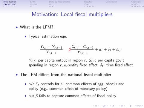
Motivation: Local �scal multipliers
� What is the LFM?
� Typical estimation eqn.
Yr ,t � Yr ,t�1Yr ,t�1
= βGr ,t � Gr ,t�1Yr ,t�1
+ αr + δt + εr ,t
Yr ,t : per capita output in region r , Gr ,t : per capita gov�tspending in region r , αr :entity �xed e¤ect, δt : time �xed e¤ect
� The LFM di¤ers from the national �scal multiplier
� b/c δt controls for all common e¤ects of agg. shocks andpolicy (e.g., common e¤ect of monetary policy)
� but β fails to capture common e¤ects of �scal policy

Introduction LFM Data & Instruments Results Conclusion Appendix
Motivation: Spillover
� Another important di¤erence from the national �scalmultiplier
� An interpretation
� Fiscal multiplier of gov�t spending in an economy in amonetary union (e.g., EU countries)
� Within a single country, ...
� Strong interdependence without the border e¤ect
� Gov�t spending may easily spill over into other economies

Introduction LFM Data & Instruments Results Conclusion Appendix
Research questions1. How large is the LFM in Japan?
� We provide estimates of LFM, comparable to other countries
2. How large is the spillover within the region?
� Positive if there is a leakage in demand
� Negative if production factors (e.g., labor) relocate acrossprefectures
3. How large is the LFM on expenditure components of GDP?
� Crowding-out or crowding-in?
� Spillover in expenditure components
Introduction LFM Data & Instruments Results Conclusion Appendix
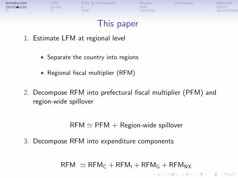
This paper
1. Estimate LFM at regional level
� Separate the country into regions
� Regional �scal multiplier (RFM)
2. Decompose RFM into prefectural �scal multiplier (PFM) andregion-wide spillover
RFM ' PFM + Region-wide spillover
3. Decompose RFM into expenditure components
RFM ' RFMC + RFMI + RFMG + RFMNX
Introduction LFM Data & Instruments Results Conclusion Appendix
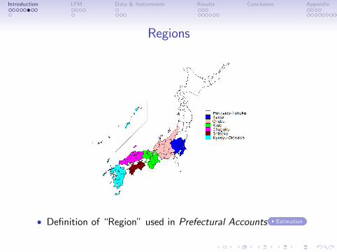
Regions
� De�nition of �Region�used in Prefectural Accounts Estimation

Introduction LFM Data & Instruments Results Conclusion Appendix
Why Japan?
� Prefectural accounts in JPN are constructed in a way highlycomparable to the national account
� Cabinet O¢ ce in JPN publishes C , I , G and NX at theprefectural level
� BEA in the US does not publish I , G and NX at thestate/county level
Introduction LFM Data & Instruments Results Conclusion Appendix
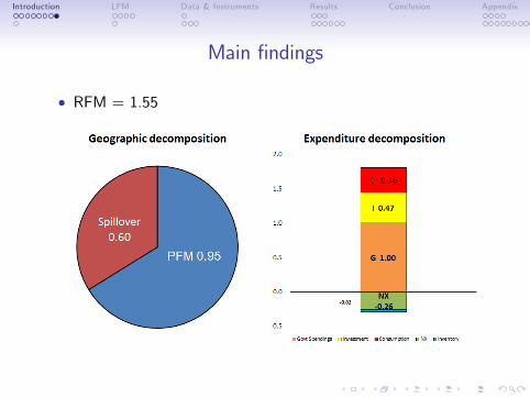
Main �ndings
� RFM = 1.55
Introduction LFM Data & Instruments Results Conclusion Appendix
Main �ndings
� RFM = 1.55

Introduction LFM Data & Instruments Results Conclusion Appendix
Literature on local �scal multipliers
� Most studies are based on the US state/county
� ARRA papers estimate �Jobs-multiplier� and �cost-per-job�� using state-level employment data of BLS� Chorodow-Reich et al. (2012), Conley and Dupor (2013),Wilson (2012), Dupor and McCroy (2017) among others
� Non-ARRA papers focus on output multiplier or incomemultipliers
� Nakamura and Steinsson (2014), Clemens and Miran (2012),Shoag (2016), Suárez-Serrato and Wingender (2016)
� International evidence
� Japan: Brückner and Tuladhar (2014) focus on the 1990s andrelationship with �nancial distress
� Italy: Acconcia et al. (2014), China: Guo et al. (2016)
� Our focus: spillover and expenditure components

Introduction LFM Data & Instruments Results Conclusion Appendix
Empirical strategy
Introduction LFM Data & Instruments Results Conclusion Appendix
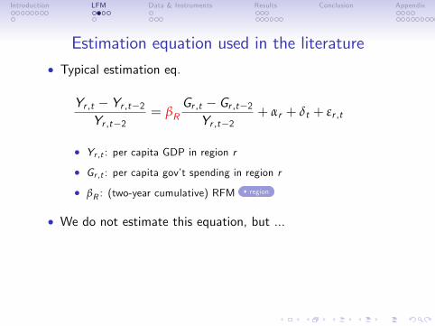
Estimation equation used in the literature� Typical estimation eq.
Yr ,t � Yr ,t�2Yr ,t�2
= βRGr ,t � Gr ,t�2Yr ,t�2
+ αr + δt + εr ,tABCDE
� Yr ,t : per capita GDP in region r
� Gr ,t : per capita gov�t spending in region r
� βR : (two-year cumulative) RFM region
� We do not estimate this equation, but ...
Introduction LFM Data & Instruments Results Conclusion Appendix
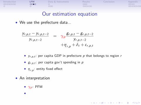
Our estimation equation� We use the prefecture data...
yr ,p,t � yr ,p,t�2yr ,p,t�2
= γPgr ,p,t � gr ,p,t�2
yr ,p,t�2+ γS
Gr ,t � Gr ,t�2Yr ,t�2
+ηr ,p + δt + εr ,p,t
� yr ,p,t : per capita GDP in prefecture p that belongs to region r
� gr ,p,t : per capita gov�t spending in p
� ηr ,p : entity �xed e¤ect
� An interpretation
� γP : PFM
� γS : region-wide spillover
Introduction LFM Data & Instruments Results Conclusion Appendix
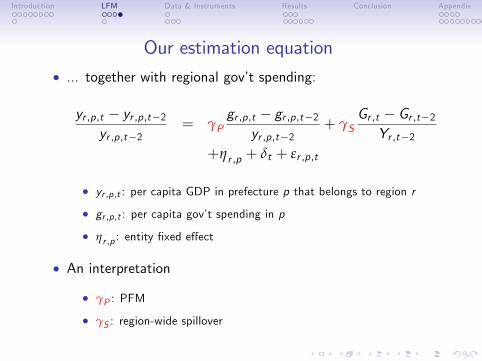
Our estimation equation� ... together with regional gov�t spending:
yr ,p,t � yr ,p,t�2yr ,p,t�2
= γPgr ,p,t � gr ,p,t�2
yr ,p,t�2+ γS
Gr ,t � Gr ,t�2Yr ,t�2
+ηr ,p + δt + εr ,p,t
� yr ,p,t : per capita GDP in prefecture p that belongs to region r
� gr ,p,t : per capita gov�t spending in p
� ηr ,p : entity �xed e¤ect
� An interpretation
� γP : PFM
� γS : region-wide spillover
Introduction LFM Data & Instruments Results Conclusion Appendix
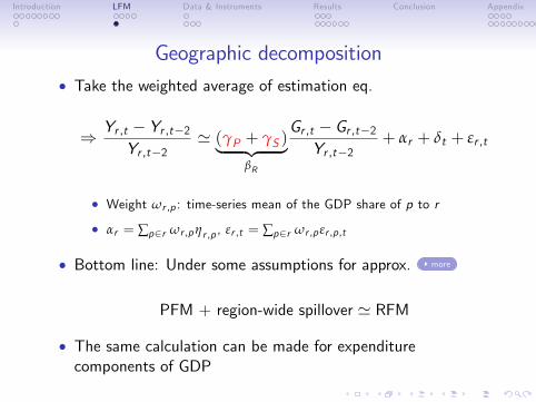
Geographic decomposition� Take the weighted average of estimation eq.
) Yr ,t � Yr ,t�2Yr ,t�2
' (γP + γS )| {z }βR
Gr ,t � Gr ,t�2Yr ,t�2
+ αr + δt + εr ,t
� Weight ωr ,p : time-series mean of the GDP share of p to r
� αr = ∑p2r ωr ,pηr ,p , εr ,t = ∑p2r ωr ,p εr ,p,t
� Bottom line: Under some assumptions for approx. more
PFM + region-wide spillover ' RFM
� The same calculation can be made for expenditurecomponents of GDP
Introduction LFM Data & Instruments Results Conclusion Appendix
Data and Instruments

Introduction LFM Data & Instruments Results Conclusion Appendix
Data� Sample period: 1990 �2012
� Annual Report on Prefectural Accounts
� Annual Statistical Report on Local Government Finance
� 7 regions and 47 prefectures
� Local gov�t spending: more
� Gov�t consumption + public investment
� e.g., Blanchard and Perotti (2002)

Introduction LFM Data & Instruments Results Conclusion Appendix
Instruments: Treasury disbursements
� Gov�t spending is endogenous
� To instrument gov�t spending, we use cross-sectionalvariations in treasury disbursements
� Transfers from the central gov�t

Introduction LFM Data & Instruments Results Conclusion Appendix
Why treasury disbursements?
1. Important revenue source for the local gov�t
� Large vertical �scal gap btwn the central and local gov�ts
2. Financed by national tax revenue pooled by the central gov�t
� unlikely to be a¤ected by local business cycle
3. Program-based transfers
� e.g., Grants for compulsory education, public health,construction (roads, ports, rivers, ...)
� Some grants are mandatory by the Local Public Law
� Other grants are discretionary, but the outline of programs isdetermined by the central gov�t, not by local gov�t
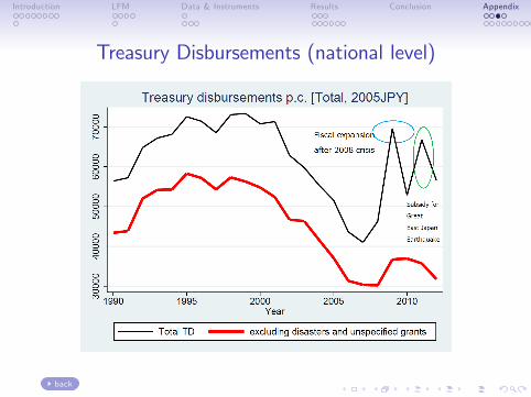
� We can remove transfers associated with local business cycle(e.g., Great East Japan earthquake) in constructing instrument

Introduction LFM Data & Instruments Results Conclusion Appendix
Why treasury disbursements?
1. Important revenue source for the local gov�t
� Large vertical �scal gap btwn the central and local gov�ts
2. Financed by national tax revenue pooled by the central gov�t
� unlikely to be a¤ected by local business cycle
3. Program-based transfers
� e.g., Grants for compulsory education, public health,construction (roads, ports, rivers, ...)
� Some grants are mandatory by the Local Public Law
� Other grants are discretionary, but the outline of programs isdetermined by the central gov�t, not by local gov�t
� We can remove transfers associated with local business cycle(e.g., Great East Japan earthquake) in constructing instrument
Introduction LFM Data & Instruments Results Conclusion Appendix
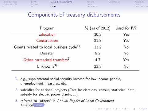
Components of treasury disbursements
Program % (as of 2012) Used for IV?
Education 30.3 Yes
Construction 21.3 Yes
Grants related to local business cycle1) 11.2 No
Disaster 9.2 No
Other earmarked transfers2) 4.7 Yes
Unknowns3) 23.3 No
1. e.g., supplemental social security income for low income people,unemployment measures, etc.
2. subsidies for national projects (Cost for elections, census, statistical data,subsidy for electric power plants, ...)
3. referred to �others� in Annual Report of Local GovernmentFinance graph

Introduction LFM Data & Instruments Results Conclusion Appendix
Results
Introduction LFM Data & Instruments Results Conclusion Appendix
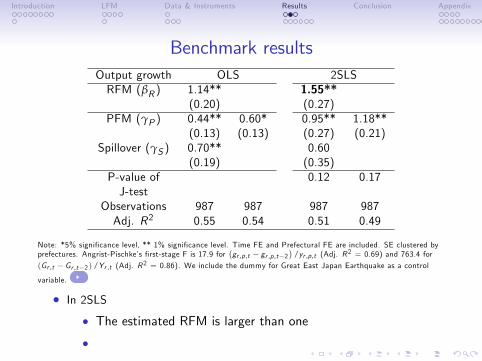
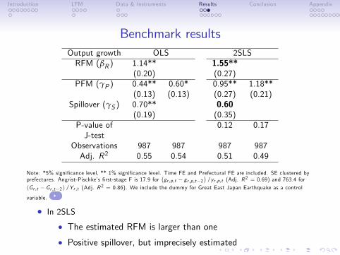
Benchmark resultsOutput growth OLS 2SLSRFM (βR ) 1.14** 1.55**
(0.20) (0.27)PFM (γP ) 0.44** 0.60* 0.95** 1.18**
(0.13) (0.13) (0.27) (0.21)Spillover (γS ) 0.70** 0.60
(0.19) (0.35)P-value of 0.12 0.17J-test
Observations 987 987 987 987Adj. R2 0.55 0.54 0.51 0.49
Note: *5% signi�cance level, ** 1% signi�cance level. Time FE and Prefectural FE are included. SE clustered byprefectures. Angrist-Pischke�s �rst-stage F is 17.9 for
�gr ,p,t � gr ,p,t�2
�/yr ,p,t (Adj. R2 = 0.69) and 763.4 for
(Gr ,t � Gr ,t�2 ) /Yr ,t (Adj. R2 = 0.86). We include the dummy for Great East Japan Earthquake as a control
variable.
� In 2SLS
� The estimated RFM is larger than one
� Positive spillover, but imprecisely estimated
Introduction LFM Data & Instruments Results Conclusion Appendix
Expenditure components in GDP
� RFM =1.55
� Crowding-in e¤ect must be observed
� What expenditure components?
Introduction LFM Data & Instruments Results Conclusion Appendix
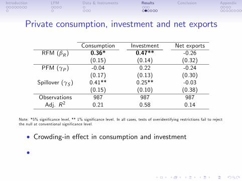
Private consumption, investment and net exports
Consumption Investment Net exportsRFM (βR ) 0.36* 0.47** -0.26
(0.15) (0.14) (0.32)PFM (γP ) -0.04 0.22 -0.24
(0.17) (0.13) (0.30)Spillover (γS ) 0.41** 0.25** -0.03
(0.15) (0.10) (0.38)Observations 987 987 987Adj. R2 0.21 0.58 0.14
Note: *5% signi�cance level, ** 1% signi�cance level. In all cases, tests of overidentifying restrictions fail to rejectthe null at conventional signi�cance level.
� Crowding-in e¤ect in consumption and investment
� Spillover is economically and statistically signi�cant inconsumption and investment
Introduction LFM Data & Instruments Results Conclusion Appendix
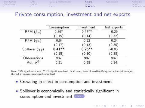
Private consumption, investment and net exports
Consumption Investment Net exportsRFM (βR ) 0.36* 0.47** -0.26
(0.15) (0.14) (0.32)PFM (γP ) -0.04 0.22 -0.24
(0.17) (0.13) (0.30)Spillover (γS ) 0.41** 0.25** -0.03
(0.15) (0.10) (0.38)Observations 987 987 987Adj. R2 0.21 0.58 0.14
Note: *5% signi�cance level, ** 1% signi�cance level. In all cases, tests of overidentifying restrictions fail to rejectthe null at conventional signi�cance level.
� Crowding-in e¤ect in consumption and investment
� Spillover is economically and statistically signi�cant inconsumption and investment More
Introduction LFM Data & Instruments Results Conclusion Appendix
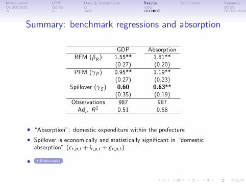
Summary: benchmark regressions and absorption
GDP AbsorptionRFM (βR ) 1.55** 1.81**
(0.27) (0.20)PFM (γP ) 0.95** 1.19**
(0.27) (0.23)Spillover (γS ) 0.60 0.63**
(0.35) (0.19)Observations 987 987Adj. R2 0.51 0.58
� �Absorption�: domestic expenditure within the prefecture
� Spillover is economically and statistically signi�cant in �domesticabsorption� (cr ,p,t + ir ,p,t + gr ,p,t )
� Robustness

Introduction LFM Data & Instruments Results Conclusion Appendix
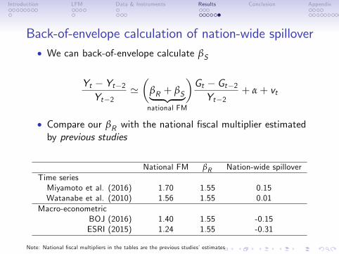
Back-of-envelope calculation of nation-wide spillover
� Consider a hypothetical eq.
Yr ,t � Yr ,t�2Yr ,t�2
= βRGr ,t � Gr ,t�2Yr ,t�2
+ βSGt � Gt�2Yt�2
+ αr + vr ,t
where Gt denotes the national gov�t spending andβS =nation-wide spillover
� βS is very di¢ cult to identify because we cannot usetime-�xed e¤ect
Introduction LFM Data & Instruments Results Conclusion Appendix
Back-of-envelope calculation of nation-wide spillover� We can back-of-envelope calculate βS
Yt � Yt�2Yt�2
'�
βR + βS| {z }�
national FM
Gt � Gt�2Yt�2
+ α+ vt
� Compare our βR with the national �scal multiplier estimatedby previous studies
National FM βR Nation-wide spilloverTime seriesMiyamoto et al. (2016) 1.70 1.55 0.15Watanabe et al. (2010) 1.56 1.55 0.01
Macro-econometricBOJ (2016) 1.40 1.55 -0.15ESRI (2015) 1.24 1.55 -0.31
Note: National �scal multipliers in the tables are the previous studies�estimates
Introduction LFM Data & Instruments Results Conclusion Appendix
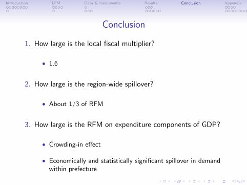
Conclusion
1. How large is the local �scal multiplier?
� 1.6
2. How large is the region-wide spillover?
� About 1/3 of RFM
3. How large is the RFM on expenditure components of GDP?
� Crowding-in e¤ect
� Economically and statistically signi�cant spillover in demandwithin prefecture
Introduction LFM Data & Instruments Results Conclusion Appendix
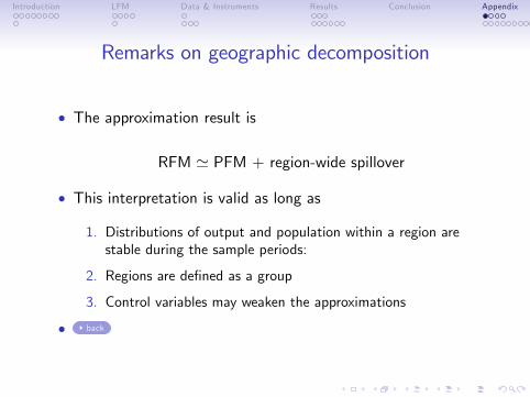
Remarks on geographic decomposition
� The approximation result is
RFM ' PFM + region-wide spillover
� This interpretation is valid as long as
1. Distributions of output and population within a region arestable during the sample periods:
2. Regions are de�ned as a group
3. Control variables may weaken the approximations
� back

Introduction LFM Data & Instruments Results Conclusion Appendix
Remarks on gov�t spending1. Our de�nition
� gr ,p,t =gov�t consumption + public investment
� Similar results when gr ,p,t = public investment
2. Due to lack of data, gov�t spending
� gr ,p,t =local gov�t spending + direct spending in p by centralgov�t
� On average, 60% of spending are made local governments(prefectures + municipalities) and 40% is made by the centralgov�t
back
Introduction LFM Data & Instruments Results Conclusion Appendix
Treasury Disbursements (national level)
back
Introduction LFM Data & Instruments Results Conclusion Appendix
Hypothesis
� Small PFM due to two o¤setting e¤ects
1. Expenditure-switching e¤ect
� Increase in gr ,p,t )Increase in domestic relative prices)Decline in domestic demand
2. Income e¤ects on liquidity constrained agents
� Increase in gr ,p,t ) Increase in domestic demand
� Large region-wide spillover due to complementary e¤ects1. Expenditure-switching e¤ect
� Increase in Gr ,t ) Decline in domestic relativeprices)Increase in demand for domestic goods
2. Income e¤ects
� Increase in Gr ,t ) Leakage in demand )Increase in income)Increase in demand for domestic goods
back
Introduction LFM Data & Instruments Results Conclusion Appendix
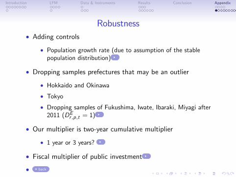
Robustness� Adding controls
� Population growth rate (due to assumption of the stablepopulation distribution)
� Dropping samples prefectures that may be an outlier
� Hokkaido and Okinawa
� Tokyo
� Dropping samples of Fukushima, Iwate, Ibaraki, Miyagi after2011 (DEr ,p,t = 1)
� Our multiplier is two-year cumulative multiplier
� 1 year or 3 years?
� Fiscal multiplier of public investment
� back
Introduction LFM Data & Instruments Results Conclusion Appendix
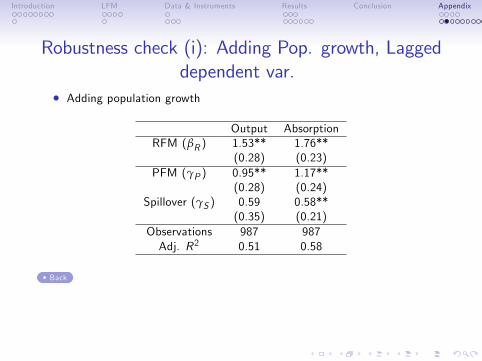
Robustness check (i): Adding Pop. growth, Laggeddependent var.
� Adding population growth
Output AbsorptionRFM (βR ) 1.53** 1.76**
(0.28) (0.23)PFM (γP ) 0.95** 1.17**
(0.28) (0.24)Spillover (γS ) 0.59 0.58**
(0.35) (0.21)Observations 987 987Adj. R2 0.51 0.58
Back
Introduction LFM Data & Instruments Results Conclusion Appendix
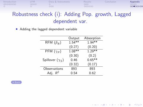
Robustness check (i): Adding Pop. growth, Laggeddependent var.
� Adding the lagged dependent variable
Output AbsorptionRFM (βR ) 1.54** 1.94**
(0.27) (0.20)PFM (γP ) 1.08** 1.29**
(0.30) (0.2)Spillover (γS ) 0.46 0.65**
(0.32) (0.17)Observations 893 893Adj. R2 0.54 0.62
Back

Introduction LFM Data & Instruments Results Conclusion Appendix
Robustness check (i): Adding Pop. growth, Laggeddependent var.
� Adding the population growth and lagged dependent variable
Output AbsorptionRFM (βR ) 1.46** 1.87**
(0.25) (0.21)PFM (γP ) 1.06** 1.27**
(0.29) (0.22)Spillover (γS ) 0.40 0.60**
(0.30) (0.19)Observations 893 893Adj. R2 0.54 0.63
Back

Introduction LFM Data & Instruments Results Conclusion Appendix
Robustness check (ii): Dropping samples...� Dropping Hokkaido and Okinawa
Output AbsorptionRFM (βR ) 1.62** 1.72**
(0.29) (0.20)PFM (γP ) 1.03** 1.07**
(0.25) (0.24)Spillover (γS ) 0.59 0.65**
(0.37) (0.20)Observations 945 945Adj. R2 0.51 0.60
� Hokkaido and Okinawa: the most northern and southern islands of JPN
Back
Introduction LFM Data & Instruments Results Conclusion Appendix
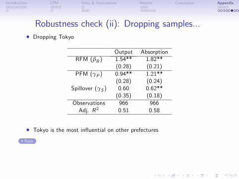
Robustness check (ii): Dropping samples...� Dropping Tokyo
Output AbsorptionRFM (βR ) 1.54** 1.82**
(0.28) (0.21)PFM (γP ) 0.94** 1.21**
(0.28) (0.24)Spillover (γS ) 0.60 0.62**
(0.35) (0.18)Observations 966 966Adj. R2 0.51 0.58
� Tokyo is the most in�uential on other prefectures
Back
Introduction LFM Data & Instruments Results Conclusion Appendix
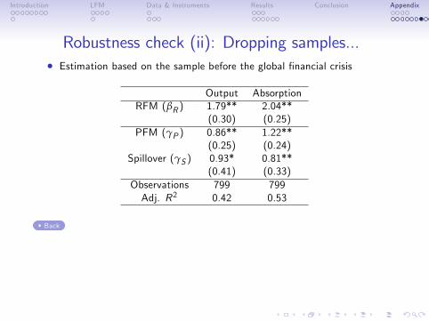
Robustness check (ii): Dropping samples...� Estimation based on the sample before the global �nancial crisis
Output AbsorptionRFM (βR ) 1.79** 2.04**
(0.30) (0.25)PFM (γP ) 0.86** 1.22**
(0.25) (0.24)Spillover (γS ) 0.93* 0.81**
(0.41) (0.33)Observations 799 799Adj. R2 0.42 0.53
Back
Introduction LFM Data & Instruments Results Conclusion Appendix
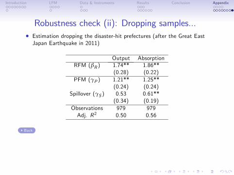
Robustness check (ii): Dropping samples...� Estimation dropping the disaster-hit prefectures (after the Great EastJapan Earthquake in 2011)
Output AbsorptionRFM (βR ) 1.74** 1.86**
(0.28) (0.22)PFM (γP ) 1.21** 1.25**
(0.24) (0.24)Spillover (γS ) 0.53 0.61**
(0.34) (0.19)Observations 979 979Adj. R2 0.50 0.56
Back
Introduction LFM Data & Instruments Results Conclusion Appendix
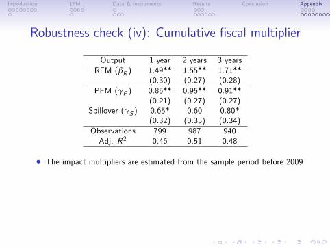
Robustness check (iv): Cumulative �scal multiplier
Output 1 year 2 years 3 yearsRFM (βR ) 1.49** 1.55** 1.71**
(0.30) (0.27) (0.28)PFM (γP ) 0.85** 0.95** 0.91**
(0.21) (0.27) (0.27)Spillover (γS ) 0.65* 0.60 0.80*
(0.32) (0.35) (0.34)Observations 799 987 940Adj. R2 0.46 0.51 0.48
� The impact multipliers are estimated from the sample period before 2009
Introduction LFM Data & Instruments Results Conclusion Appendix
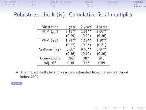
Robustness check (iv): Cumulative �scal multiplier
Absorption 1 year 2 years 3 yearsRFM (βR ) 2.15** 1.81** 2.06**
(0.29) (0.20) (0.26)PFM (γP ) 1.29** 1.19** 1.20**
(0.27) (0.23) (0.21)Spillover (γS ) 0.86* 0.63** 0.86**
(0.36) (0.19) (0.26)Observations 799 987 940Adj. R2 0.45 0.58 0.59
� The impact multipliers (1 year) are estimated from the sample periodbefore 2009
Back
Introduction LFM Data & Instruments Results Conclusion Appendix
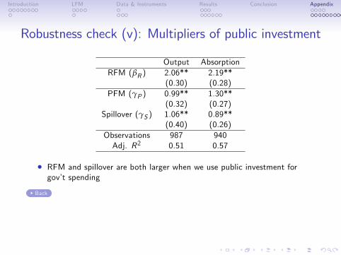
Robustness check (v): Multipliers of public investment
Output AbsorptionRFM (βR ) 2.06** 2.19**
(0.30) (0.28)PFM (γP ) 0.99** 1.30**
(0.32) (0.27)Spillover (γS ) 1.06** 0.89**
(0.40) (0.26)Observations 987 940Adj. R2 0.51 0.57
� RFM and spillover are both larger when we use public investment forgov�t spending
Back
Introduction LFM Data & Instruments Results Conclusion Appendix
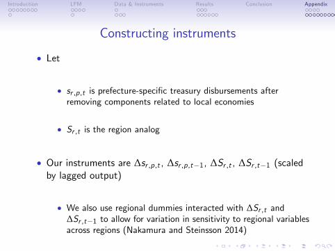
Constructing instruments
� Let
� sr ,p,t is prefecture-speci�c treasury disbursements afterremoving components related to local economies
� Sr ,t is the region analog
� Our instruments are ∆sr ,p,t , ∆sr ,p,t�1, ∆Sr ,t , ∆Sr ,t�1 (scaledby lagged output)
� We also use regional dummies interacted with ∆Sr ,t and∆Sr ,t�1 to allow for variation in sensitivity to regional variablesacross regions (Nakamura and Steinsson 2014)
Introduction LFM Data & Instruments Results Conclusion Appendix
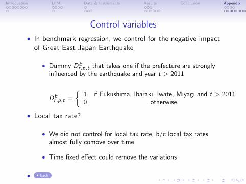
Control variables� In benchmark regression, we control for the negative impactof Great East Japan Earthquake
� Dummy DEr ,p,t that takes one if the prefecture are stronglyin�uenced by the earthquake and year t > 2011
DEr ,p,t =�1 if Fukushima, Ibaraki, Iwate, Miyagi and t > 20110 otherwise.
� Local tax rate?
� We did not control for local tax rate, b/c local tax ratesalmost fully comove over time
� Time �xed e¤ect could remove the variations
� back