ISSN (Print) 0473-453X Discussion Paper No. 1065 ISSN (Online) 2435-0982

DECOMPOSING LOCAL FISCAL MULTIPLIERS:

EVIDENCE FROM JAPAN

Taisuke Kameda Ryoichi Namba

Takayuki Tsuruga

October 2019

The Institute of Social and Economic Research Osaka University

6-1 Mihogaoka, Ibaraki, Osaka 567-0047, Japan

Decomposing Local Fiscal Multipliers: Evidence from Japan∗

Taisuke Kameda† Ryoichi Namba‡, Takayuki Tsuruga§

First draft: July 2017

This draft: October 2019

Abstract

Recent studies on fiscal policy use cross-sectional data and estimate local fiscal multipliers

along with spillovers. This paper estimates local fiscal multipliers with spillovers using Japanese

prefectural data comparable with the national accounts. We estimate the local fiscal multiplier

on output to be 1.7 at the regional level. The regional fiscal multiplier consists of the prefecture-

specific components and a component common across prefectures within the same region, which

we interpret as the region-wide effect. Converting the latter component into the spillover, we find

that the spillover is positive and small in size. We decompose the regional fiscal multiplier on

output into multipliers on expenditure components. The regional fiscal multiplier on absorption

exceeds 2.0 because of the crowding-in effect on consumption and investment. Moreover, we

find that the spillover to absorption is considerable in contrast to the spillover to output.

JEL Classification: E62, H30, R50

Keywords: Fiscal stimulus, spillover, geographic cross-sectional fiscal multiplier

∗We thank Andrew Hallett, Hirokazu Ishise, Yasushi Iwamoto, Yi Lu, Jun Nagayasu, Etsuro Shioji, Justin Wolfers,Lianming Zhu, and seminar and conference participants at Osaka University, Shanghai University of InternationalBusiness and Economics, the University of Tokyo, the 19th Macroeconomic Conference, the Economic and SocialResearch Institute international conference, and the WEAI international conference for helpful discussions and com-ments. Takayuki Tsuruga gratefully acknowledges the financial support of Grants-in-aid for Scientific Research(15H05729 and 15H05728), the Murata Science Foundation, and the Zengin Foundation for Studies on Economicsand Finance. The views expressed in this paper are those of the authors and do not necessarily reflect the officialviews of the Government of Japan.†Cabinet Office, the Government of Japan‡Chubu Region Institute for Social and Economic Research§Osaka University; Cabinet Office, the Government of Japan; Centre for Applied Macroeconomic Analysis

1

1 Introduction

One of the cornerstone issues of macroeconomics is the interaction of economic activity and govern-

ment spending. This interaction is often measured by the fiscal multiplier, the percentage increase

in output when government spending increases by 1% of gross domestic product (GDP). Although

the literature traditionally measures the fiscal multiplier using time-series data, recent studies rely

on geographic cross-sectional variations in government spending. The fiscal multiplier estimated

from the regional cross-sectional data is often called the local fiscal multiplier (LFM). 1 Although

the LFM can be interpreted as a fiscal multiplier that measures the effect of government spend-

ing in one region within a monetary union (Nakamura and Steinsson 2014), the LFM differs from

the traditional national fiscal multiplier in an important dimension. In particular, because local

economies have strong interdependence without the border effect, government spending in a local

economy can easily spill over into other local economies. According to Auerbach et al. (2019),

understanding the spillover from government spending is “a fundamental and largely unresolved

task in macroeconomics.”

In this paper, we estimate and decompose the LFM to understand the spillover in local economies.

The objectives of this paper are threefold. First, we provide evidence of the LFM in Japan, which

we can compare with LFMs in other countries. Second, and more importantly, we measure the

spillover within the region using prefectural data. We separate the country into regions consisting

of prefectures and estimate the regional fiscal multiplier (RFM) as the sum of the prefectural fis-

cal multiplier (PFM) and the region-wide effect. The former is a component of the RFM that is

estimated from variations in prefectural government spending. The latter is also a component of

the RFM but is estimated from variations in regional government spending and, thus, it is related

to the spillover. To be consistent with the literature, we convert the estimated region-wide effect

into the spillover within the region and assess the contribution of the spillover to the RFM. Third,

exploiting an advantage of Japanese prefectural data, we estimate the RFM on the expenditure

components of GDP. The prefectural data are drawn from the “prefectural accounts,” which are

highly comparable with the national accounts, as data on consumption, investment, government

spending, and net exports are available at the prefectural level. The data availability contrasts

1Chodorow-Reich (2019) comprehensively reviews numerous recent studies on the LFM. Ramey (2011) surveysfiscal and tax multipliers including the time-series evidence.

2

with the U.S. state-level data published by the Bureau of Economic Analysis.2 Exploiting the data

compiled by the single government agency, we measure the contribution of the RFM on expenditure

components, such as private consumption and investment, to the RFM on output. Based on this

decomposition, we study which expenditure components of GDP are crowded out or in by local

government spending.

As the previous studies on the fiscal multiplier emphasize, identifying fiscal multipliers requires

isolating changes in government spending that are uncorrelated with shocks to the local economy.

We construct instruments from the national treasury disbursements in the local public finance

data.3 The expenditure by the local governments depends heavily on the transfers from the central

government because of the large vertical fiscal gap between the central and local governments (see

Bessho 2016). The national treasury disbursements are the earmarked, program-based transfers

from the central government to the local government. By definition, the national treasury disburse-

ments are financed by the national tax revenues, which are less likely to be affected by shocks to

specific prefectures’ economic activity. Furthermore, the data set allows us to identify purposes

and programs supported by the disbursements (e.g., education, social welfare, and construction).

Using the detailed information on the local public finance data, we exclude the transfers that are

strongly correlated with shocks to local economies (e.g., subsidies for recovery from disasters) in

constructing our instruments.

The main findings are as follows. First, when government spending increases at the regional

level by 1% of GDP, the regional output increases by 1.7%. In other words, the RFM on output

is 1.7. Second, we find that the spillover to output is positive but small in size. Our benchmark

estimation suggests that the spillover converted from the region-wide effect is, on average, 0.26,

out of the estimated RFM of 1.7. Third, regional government spending substantially crowds in

private consumption and private fixed investment. In particular, the sum of the contributions of

these expenditure components accounts for 65% of the RFM on output. As a result, the multiplier

on “domestic absorption” or the expenditure before the leakage to the other local economies is

2For example, the Bureau of Economic Analysis does not publish data on net exports and business investment atthe state level. In the literature on the LFM in the U.S., data for state-level government spending are often takenfrom the U.S. Census Bureau.

3Our approach is similar to Kraay (2012) and Guo et al. (2016), who use variations in the funds loaned ortransferred from an organization other than the local government for identification. Kraay (2012) estimates the fiscalmultiplier in developing countries with the instrument of World Bank lending. Guo et al. (2016) estimate the LFMin China. To identify the LFM, they use the local public finance fact that poor Chinese counties receive preferentialearmarked treatment in transfers.

3

also large. We find that the RFM on absorption is 2.2 in the benchmark regression. We also find

that the region-wide effect on absorption is statistically and economically significant, in contrast to

that on output. Our estimation suggests that the spillover converted from the region-wide effect

is, on average, 0.68, out of the estimated RFM on absorption of 2.2. By contrast, net exports

decrease with regional government spending, suggesting a leakage in aggregate demand to other

local economies.

The literature on the LFM is very active, with contributions from many previous studies.4 Some

studies focus on spillovers in the context of the LFM. Dupor and McCrory (2017) discover evidence

for positive spillovers in wage bills and employment within the regional market. Dupor and Guerrero

(2017), using federal defense contracts at the U.S. state level, find a positive interstate spillover

in income and employment multipliers. Auerbach et al. (2019) also use the U.S. federal defense

data and find positive spillovers across industries, as well as across locations. Suarez-Serrato and

Wingender (2016) explore the income spillovers across neighboring counties but find no evidence

of sizable spillovers. Acconcia et al. (2014) use Italian provincial data and find a statistically

insignificant spillover to the provincial output. Our paper studies the spillover more closely than

these previous studies by examining the expenditure components of GDP, as well as output. Guo

et al. (2016) investigate Chinese county-level data and estimate the LFM on investment at the

county level as well as output. They find that there is a crowding-in effect on investment without

assuming spillovers. Cohen et al. (2011) also estimate the impact of state government spending on

investment by publicly traded U.S. firms. They find negative impacts of local government spending

on firms’ investment and payouts to the investors of firms.

Bruckner and Tuladhar (2014) and Bessho (2018) provide evidence on the estimated LFM in

Japan. The former focuses on the financial distress of the 1990s and its impact on the LFM and the

latter examines whether the LFM is related to ageing that varies across prefectures. Other previous

studies on the Japanese fiscal multipliers provide time-series evidence.5 Among these time-series-

based studies, recent works emphasize the state dependence of the national fiscal multipliers.6

4Examples of earlier works include Clemens and Miran (2012), Nakamura and Steinsson (2014), Fishback andKachanovskaya (2015), Shoag (2016), and Suarez-Serrato and Wingender (2016). Regarding the impact of theAmerican Recovery and Reinvestment Act on employment at the state and county levels, see Chodorow-Reich et al.(2012), Wilson (2012), and Conley and Dupor (2013) among others.

5For example, Watanabe et al. (2010) estimate the national fiscal multipliers using a structural vector autoregres-sion approach that is similar to Blanchard and Perotti (2002).

6See Morita (2015), Auerbach and Gorodnichenko (2017), Kato et al. (2018), and Miyamoto et al. (2018).

4

This paper is organized as follows. Section 2 describes the empirical strategies. In Section 3,

we discuss the data and the construction of instruments. Section 4 presents the main results and

section 5 shows robustness. Section 6 concludes.

2 Local fiscal multipliers and the region-wide effect

In the existing literature, the LFM is typically estimated using the following equation:

Yr,t − Yr,t−2Yr,t−2

= βRGr,t −Gr,t−2

Yr,t−2+ αr + δt + εr,t, (1)

where Yr,t is the regional-level per capita output in period t and Gr,t is the regional-level per capita

government spending. We refer to βR as the regional fiscal multiplier (RFM) because we estimate

βR using the regional-level data. The index r represents regions in a country, r ∈ {r1, r2, ..., rM},

where the country has M regions. Note that αr and δt include the entity and time fixed effects,

respectively. For now, we assume no covariates to simplify the discussion, but our empirical analysis

includes covariates. The error term is εr,t. The entity fixed effect αr controls for the region-specific

variations in per capita output and government spending. The time fixed effect δt captures the

unobserved nationwide effects of aggregate shocks and macroeconomic policy on the regional output

(e.g., aggregate productivity, monetary policy, national tax changes, and predictable changes in the

national output and government spending). As a result of the fixed effects, βR measures how much

output in a region increases relative to that in other regions when government spending in the region

increases relative to that in other regions. The time unit is one year. Following Nakamura and

Steinsson (2014), we take the two-year growth rate of output for the dependent variable. Therefore,

βR is the two-year cumulative fiscal multiplier.

In this paper, our estimation equation takes the following prefecture analog of (1), but with an

additional regressor:

yr,p,t − yr,p,t−2yr,p,t−2

= γPgr,p,t − gr,p,t−2

yr,p,t−2+ γS

Gr,t −Gr,t−2Yr,t−2

+ ηr,p + δt + εr,p,t, (2)

where yr,p,t is per capita output and gr,p,t is per capita government spending in prefecture p, which

belongs to region r. Formally, each region ri has Ri prefectures and the index pi is defined by

5

pi ∈ ri = {1, 2, ..., Ri} for i = 1, ...,M . For notational simplicity, we drop the index i from ri and

pi in (2). As before, ηr,p captures the entity fixed effect, defined similarly to αr in (1). Note that

(2) includes changes in both prefectural and regional government spending. We interpret γP as the

prefectural fiscal multiplier (PFM) because, if γS = 0, (2) has the same structure as (1), in which we

discussed the RFM. However, if γS 6= 0, this equation indicates that the prefectural output growth

responds to changes in the regional government spending (scaled by the regional output). Even

if government spending in the prefecture stays constant, the output of the same prefecture may

change with regional government spending. Therefore, we interpret γS as the region-wide effect.

The sign of the region-wide effect γS can be positive or negative as a result of the spillover, as

discussed in the literature.7 On the one hand, an increase in government spending in a prefecture

may increase the relative price of the prefecture’s output to the same goods in other prefectures.

Thus, expenditure switches from the prefecture’s output to output in other prefectures, perhaps

those in the same region. This expenditure switching implies a positive γS . In addition, the

increase in the prefecture’s government spending may boost the demand of liquidity-constrained

households.8 If the increase in demand leaks into other prefectures in the same region, again γS

is positive. On the other hand, when the increase in government spending stimulates production

in the prefecture, it may lead to the relocation of factor inputs (e.g., labor) from other prefectures

within the same region. Because this may reduce the output in the other prefectures, the spillover

may produce a negative γS .

We show that the sum of γP and γS can approximate βR in (1). Let ωr,p be the time-series

mean of the prefecture’s GDP as a share of regional GDP. Taking the weighted average of both

sides of (2) with the GDP share ωr,p, we can approximate the equation by:

Yr,t − Yr,t−2Yr,t−2

' (γP + γS)Gr,t −Gr,t−2

Yr,t−2+ αr + δt + εr,t, (3)

where we redefine αr as the weighted average of ηr,p: αr =∑

p∈r ωr,pηr,p and the error term

εr,t =∑

p∈r ωr,pεr,p,t. Here, the derivation of the above equation requires that the distributions of

output and population are stable over the sample periods.

7For example, see Acconcia et al. (2014), Suarez-Serrato and Wingender (2016), and Chodorow-Reich (2019).8See Galı et al. (2007) for the model with liquidity-constrained households. They consider households that have

no access to capital markets. An increase in government spending that leads to higher household income can directlyincrease their consumption.

6

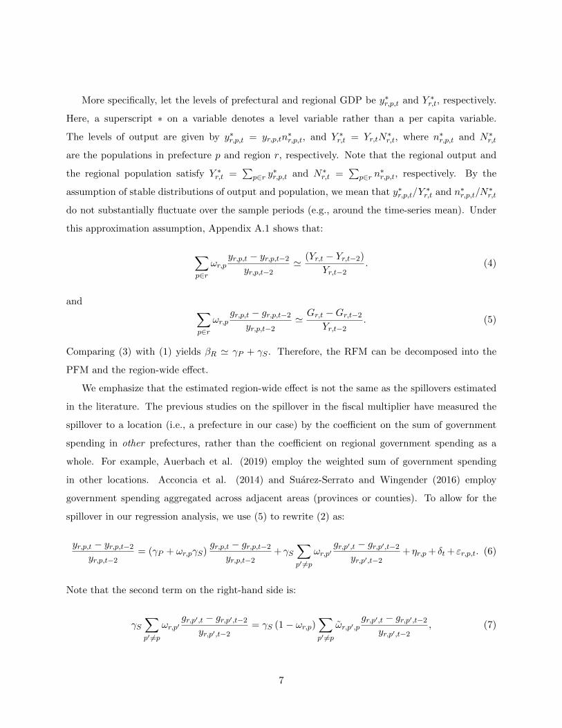
More specifically, let the levels of prefectural and regional GDP be y∗r,p,t and Y ∗r,t, respectively.

Here, a superscript ∗ on a variable denotes a level variable rather than a per capita variable.

The levels of output are given by y∗r,p,t = yr,p,tn∗r,p,t, and Y ∗r,t = Yr,tN

∗r,t, where n∗r,p,t and N∗r,t

are the populations in prefecture p and region r, respectively. Note that the regional output and

the regional population satisfy Y ∗r,t =∑

p∈r y∗r,p,t and N∗r,t =

∑p∈r n

∗r,p,t, respectively. By the

assumption of stable distributions of output and population, we mean that y∗r,p,t/Y∗r,t and n∗r,p,t/N

∗r,t

do not substantially fluctuate over the sample periods (e.g., around the time-series mean). Under

this approximation assumption, Appendix A.1 shows that:

∑p∈r

ωr,pyr,p,t − yr,p,t−2

yr,p,t−2' (Yr,t − Yr,t−2)

Yr,t−2. (4)

and ∑p∈r

ωr,pgr,p,t − gr,p,t−2

yr,p,t−2' Gr,t −Gr,t−2

Yr,t−2. (5)

Comparing (3) with (1) yields βR ' γP + γS . Therefore, the RFM can be decomposed into the

PFM and the region-wide effect.

We emphasize that the estimated region-wide effect is not the same as the spillovers estimated

in the literature. The previous studies on the spillover in the fiscal multiplier have measured the

spillover to a location (i.e., a prefecture in our case) by the coefficient on the sum of government

spending in other prefectures, rather than the coefficient on regional government spending as a

whole. For example, Auerbach et al. (2019) employ the weighted sum of government spending

in other locations. Acconcia et al. (2014) and Suarez-Serrato and Wingender (2016) employ

government spending aggregated across adjacent areas (provinces or counties). To allow for the

spillover in our regression analysis, we use (5) to rewrite (2) as:

yr,p,t − yr,p,t−2yr,p,t−2

= (γP + ωr,pγS)gr,p,t − gr,p,t−2

yr,p,t−2+ γS

∑p′ 6=p

ωr,p′gr,p′,t − gr,p′,t−2

yr,p′,t−2+ ηr,p + δt + εr,p,t. (6)

Note that the second term on the right-hand side is:

γS∑p′ 6=p

ωr,p′gr,p′,t − gr,p′,t−2

yr,p′,t−2= γS (1− ωr,p)

∑p′ 6=p

ωr,p′,pgr,p′,t − gr,p′,t−2

yr,p′,t−2, (7)

7

where ωr,p′,p = ωr,p′/ (1− ωr,p) and∑

p′ 6=p ωr,p′,p = 1. We define Yr,−p,t and Gr,−p,t by Yr,−p,t ≡

Y ∗r,−p,t/N∗r,−p,t and Gr,−p,t ≡ G∗r,−p,t/N

∗r,−p,t, respectively. Here, Y ∗r,−p,t =

∑p′ 6=p y

∗r,p′,t, G

∗r,−p,t =∑

p′ 6=p g∗r,p′,t and N∗r,−p,t =

∑p′ 6=p n

∗r,p′,t. In these definitions, we exclude prefecture p from the

weight ωr,p′,p and the aggregate variables Y ∗r,−p,t, G∗r,−p,t, and N∗r,−p,t. Under the stable distributions

of output and population, we combine (6), (7), and the above definitions to obtain:9

yr,p,t − yr,p,t−2yr,p,t−2

= (γP + ωr,pγS)gr,p,t − gr,p,t−2

yr,p,t−2+ γS (1− ωr,p)

Gr,−p,t −Gr,−p,t−2Yr,−p,t−2

(8)

+ηr,p + δt + εr,p,t.

Here, γS (1− ωr,p) is the coefficient on the sum of government spending in other prefectures, so we

interpret γS (1− ωr,p) as the measure of the spillover for prefecture p in region r. In our analysis,

we use the data on ωr,p and assess the size of the spillover.

Our measure of the spillover γS (1− ωr,p) takes into account the relative size of the local economy

in the region, whereas the previous studies assume that the degree of spillover is the same across all

local economies. More specifically, if a prefecture is large relative to the region (e.g., Tokyo in the

Kanto region), the spillover to the large local economy is low. On the other hand, if a prefecture

is small and has a negligible share in regional GDP (i.e., ωr,p ' 0), then the spillover to the small

local economy is close to γS . Put differently, the region-wide effect γS is the upper bound of the

spillover within the region.

In our empirical analysis, we estimate γP and γS from (2) and report γP + γS as an estimate of

βR. However, other factors may weaken the link between γP + γS and βR. First, we must define

the region as a group. In other words, we must have Y ∗r,t =∑

p∈r y∗r,p,t and N∗r,t =

∑p∈r n

∗r,p,t.

Second, if we include the vector of prefectural control variables xr,p,t in (2), (1) is also required to

have the vector of the control variables Xr,t =∑

p∈r ωr,pxr,p,t as additional regressors. Therefore,

to maintain the approximation results of βR ' γP +γS , the control variables in (1) are the weighted

average of the control variables across prefectures. Likewise, if (1) includes additional regressors

that are not the weighted average of prefectural control variables, the inclusion may weaken the

link between βR and γP + γS .

Regarding the control variables introduced in (2), the benchmark regression includes the dummy

variable for the Great East Japan Earthquake on March 11, 2011, the last month of fiscal year

9See Appendix A.2 for the derivation of (8).

8

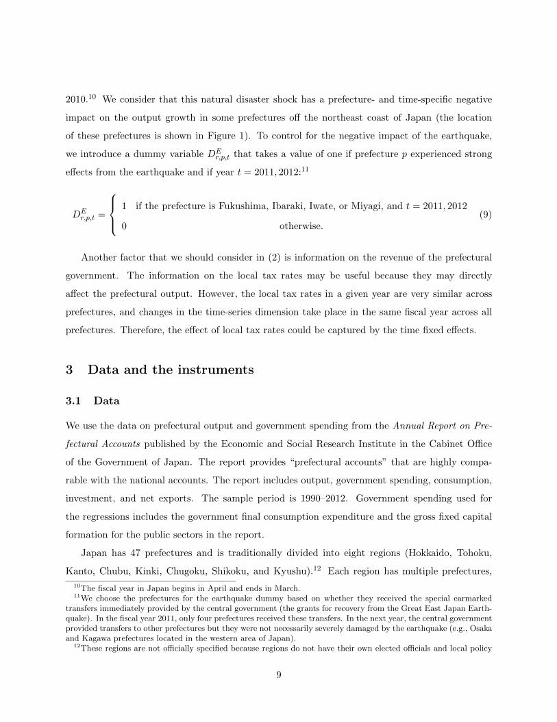
2010.10 We consider that this natural disaster shock has a prefecture- and time-specific negative

impact on the output growth in some prefectures off the northeast coast of Japan (the location

of these prefectures is shown in Figure 1). To control for the negative impact of the earthquake,

we introduce a dummy variable DEr,p,t that takes a value of one if prefecture p experienced strong

effects from the earthquake and if year t = 2011, 2012:11

DEr,p,t =

1 if the prefecture is Fukushima, Ibaraki, Iwate, or Miyagi, and t = 2011, 2012

0 otherwise.(9)

Another factor that we should consider in (2) is information on the revenue of the prefectural

government. The information on the local tax rates may be useful because they may directly

affect the prefectural output. However, the local tax rates in a given year are very similar across

prefectures, and changes in the time-series dimension take place in the same fiscal year across all

prefectures. Therefore, the effect of local tax rates could be captured by the time fixed effects.

3 Data and the instruments

3.1 Data

We use the data on prefectural output and government spending from the Annual Report on Pre-

fectural Accounts published by the Economic and Social Research Institute in the Cabinet Office

of the Government of Japan. The report provides “prefectural accounts” that are highly compa-

rable with the national accounts. The report includes output, government spending, consumption,

investment, and net exports. The sample period is 1990–2012. Government spending used for

the regressions includes the government final consumption expenditure and the gross fixed capital

formation for the public sectors in the report.

Japan has 47 prefectures and is traditionally divided into eight regions (Hokkaido, Tohoku,

Kanto, Chubu, Kinki, Chugoku, Shikoku, and Kyushu).12 Each region has multiple prefectures,

10The fiscal year in Japan begins in April and ends in March.11We choose the prefectures for the earthquake dummy based on whether they received the special earmarked

transfers immediately provided by the central government (the grants for recovery from the Great East Japan Earth-quake). In the fiscal year 2011, only four prefectures received these transfers. In the next year, the central governmentprovided transfers to other prefectures but they were not necessarily severely damaged by the earthquake (e.g., Osakaand Kagawa prefectures located in the western area of Japan).

12These regions are not officially specified because regions do not have their own elected officials and local policy

9

except for Hokkaido, located in the north of Japan. Following the Annual Report on Prefectural

Accounts, we combine Hokkaido/Tohoku into one region (see Figure 1).

As we will elaborate in the next subsections, we utilize the cross-sectional variations of transfers

from the central government to the prefectural governments in instrumenting government spending.

We take the data on the transfers from the Annual Statistical Report on Local Government Finance

published by the Ministry of Internal Affairs and Communications. All data are reported as nominal

variables. When we transform the nominal variables into real variables, we deflate them by the

prefecture-specific GDP deflator, with 2005 as the base year.

3.2 Instrumenting government spending

Government spending is endogenous. Indeed, the government spending variables gr,p,t and Gr,t are

affected by the state of the local economy, because they are a policy variable. In the estimation, the

time fixed effect can control for all aggregate shocks to the prefectural output. However, government

spending is still correlated with prefectural-specific shocks to prefectural output. For example, if

a disaster decreases output in a prefecture, the local government would increase the government

spending to recover from the disaster, relative to other prefectures that are not affected by the

disaster.

To address the endogeneity issues, we use cross-sectional variations in transfers from the central

government to the local governments. To instrument government spending with transfers, we use

the following institutional facts regarding local public finance: (i) local government spending in

Japan is highly dependent on transfers from the central government; (ii) the transfers from the

central government are financed by the national tax revenue, which is unlikely to be affected by

local business cycles; and (iii) depending on their type, the transfers are disbursed to achieve specific

national objectives and are not designed to assist the local government’s discretionary policy to

stimulate the local economy. We will discuss each institutional fact in turn below.

3.2.1 Institutional facts

(i) Local government spending depends on transfers from the central government

Government activity in Japan is highly centralized, and the local governments rely on transfers or

decisions within the same region are independent.

10

the redistribution of national tax revenue from the central government to finance their expenditure.

This dependence stems from the vertical fiscal gap between the central and local governments. Al-

though the local governments are assigned various functions by the central government, they do not

have sufficient sources of revenues to carry out their functions (see Bessho 2016). In particular, the

local governments’ expenditure accounts for about 60% of total government expenditure, but their

revenue is only 40% of the total government revenue. This large vertical fiscal gap between the cen-

tral and local governments means that transfers from the central government to local governments

are essential. In the fiscal year 2012, for example, these transfers from the central government

accounted for 34% of the total revenue of all prefectural governments. The transfers are compa-

rable in size to local tax revenues, which account for 32% of the total revenue of the prefectural

governments (Ministry of Internal Affairs and Communications 2014). These facts suggest that

there would be significant correlations between the local government spending and the transfers

from the central government.

(ii) Transfers are financed by the national tax revenue The national tax revenue finances

the transfers from the central government. By construction, the national tax revenue is unlikely

to be affected by the state of the local economies because it is pooled in the central government.

Business cycle fluctuations and the fiscal policy at the national level strongly affect the national

tax revenue. However, the time fixed effect in the regressions controls for such macroeconomic

variations over time, unless the macroeconomic shocks have heterogeneous impacts on the local

economy.

(iii) Depending on their type, the transfers are disbursed to achieve specific national

objectives The local governments in Japan broadly receive two types of transfers from the cen-

tral government: “the local allocation tax” and the “national treasury disbursements.” Although

the former accounts for a substantial fraction of the total revenue of the prefectural governments

(e.g., 18.3% in the fiscal year 2012), it is not suitable as our instrument because it is allocated to

reduce the horizontal fiscal gap across local governments. For example, when the local tax revenue

in a prefecture is lower (because of a negative shock to income in the prefecture) than in other

prefectures, the central government allocates more funds to that prefecture to reduce the imbal-

ance in the tax revenue across local governments. Therefore, the local allocation tax is likely to

11

be strongly correlated with shocks to the local economy. Likewise, if the output growth in two

prefectures within the same region is similar, transfers from the local allocation taxes are likely to

comove in these prefectures because of the similarity in changes in their tax revenue. Again, the

local allocation taxes are strongly correlated with shocks to the local economy.

For the second type of transfer from the central to local governments, (the “treasury disburse-

ments” for short), these problems are much less severe. While these transfers account for 15.6% of

the total revenue in the fiscal year 2012, the treasury disbursements are grants to promote projects

that aim to contribute to specific national objectives (e.g., education, social welfare, and social

capital constructions). To acquire the treasury disbursements, local governments prepare appli-

cations describing specific projects, with an emphasis on the necessity and earmarking of grants.

Ministries in the central government review their applications and decide whether to approve the

grants and/or subsidies. In general, it is difficult for the local government to use the grants to

implement countercyclical fiscal policy because a fiscal stimulus to specific prefectures is not nec-

essarily consistent with the national objectives. Of course, some projects supported by treasury

disbursements have purposes that relate to specific local economies. For example, the central gov-

ernment assists disaster-hit prefectures to recover from disasters (e.g., special grants to recover from

the Great East Japan Earthquake in the item of the treasury disbursement). However, the data of

the treasury disbursements includes various categories based on the grant purposes and programs.

Using this detailed information, we can remove the grants relating to the specific local economies

in constructing the instruments for the regression analysis.

3.2.2 Constructing the instruments

The Annual Statistical Report on Local Government Finance provides detailed information on the

purposes and programs of the treasury disbursements transferred to prefectures. Table 1 shows

the purposes and programs that we can identify from the report in 2012. As indicated in Table 1,

the main components of the treasury disbursements are education (30.3% of the treasury disburse-

ments), construction (21.3%), grants and subsidies that may be related to local business cycles and

countercyclical policies (12.3%), and grants for recovery from disasters (9.2%).

We look for purposes and programs of the treasury disbursements that we can keep track of

during the sample period to construct instruments. We choose three categories that are considered

12

to be uncorrelated to shocks to the local economy, based on the purposes and programs shown in

Table 1.

The first category that we choose is the treasury disbursements for education. This category

mainly includes compulsory education. The total amount of this subsidy largely depends on the

number of teachers and staff in public schools, which is prescribed by law, and on their salaries,

which are insensitive to local business cycles.13 We argue that other subsidies and grants used for

education would vary based on the prefecture’s distribution of children within the population.

The second category that we select for constructing instruments is construction, which includes

”ordinary construction” and “grants for comprehensive infrastructure development.” For example,

grants for building public facilities and infrastructure (e.g., construction and maintenance of public

facilities, road and bridges, river improvements, and coastal defenses) are included in this category.

Regarding the grants for comprehensive infrastructure development, the Ministry of Land, Infras-

tructure, Transport, and Tourism exclusively approves the infrastructure-related grants. To apply

for these types of grants, the local governments need to prepare an application describing how their

spending contributes to the national objectives.

We do not choose purposes and programs in the treasury disbursements that are strongly related

to shocks to the local economy. In particular, we do not select subsidies for livelihood protection

(i.e., supplemental social security income for low-income people) and child protection because these

subsidies depend on the number of recipients, which comoves with business cycle fluctuations at

the prefectural level. For the same reason, we do not choose the subsidy for self-support of the

disabled, though it is a more statutory subsidy than subsidies for livelihood protection and child

protection. We exclude grants for regional autonomous strategies in constructing our instruments

because local governments are permitted to use these for discretionary purposes. We do not include

disaster restoration because they are designed to stimulate the local economies.

The third category selected for constructing instruments is earmarked transfers, although these

transfers account for only 3.6% of the treasury disbursements. Among these, the subcategory of

“money in trust” corresponds to transfers to conduct national projects (e.g., national elections

and the collection of statistical and census data) and is fully funded by the central government.

Grants for locating electric power stations and petroleum reserve facilities are given to prefectures,

13The transfers from the central government for construction of school buildings and related facilities are includedwithin the construction category in the treasury disbursements.

13

depending on the extent to which such facilities exist in the prefecture. It can be assumed that

these subcategories of grants are unrelated to shocks to the local economy.

The Annual Report does not provide detailed information on other small grants, which account

for 23.3% of the treasury disbursements. The report treats these grants as ”others” and we cannot

identify their programs and purposes. Therefore, we exclude this category in constructing our

instruments.

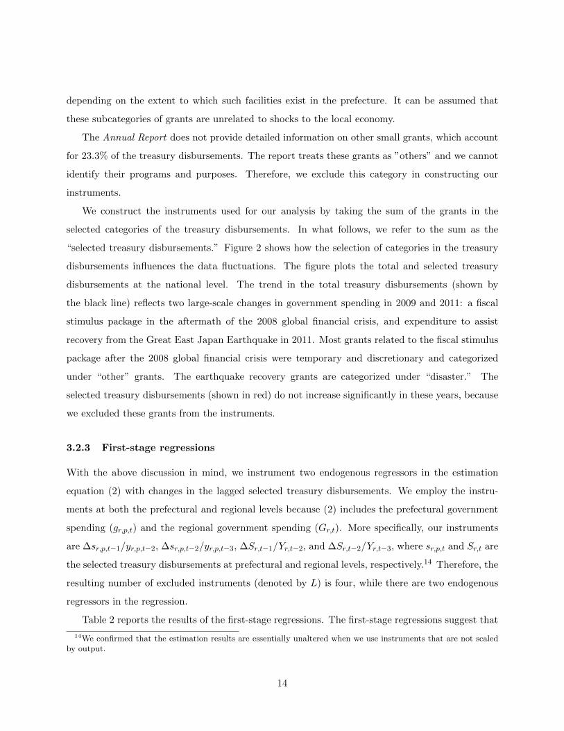
We construct the instruments used for our analysis by taking the sum of the grants in the

selected categories of the treasury disbursements. In what follows, we refer to the sum as the

“selected treasury disbursements.” Figure 2 shows how the selection of categories in the treasury

disbursements influences the data fluctuations. The figure plots the total and selected treasury

disbursements at the national level. The trend in the total treasury disbursements (shown by

the black line) reflects two large-scale changes in government spending in 2009 and 2011: a fiscal

stimulus package in the aftermath of the 2008 global financial crisis, and expenditure to assist

recovery from the Great East Japan Earthquake in 2011. Most grants related to the fiscal stimulus

package after the 2008 global financial crisis were temporary and discretionary and categorized

under “other” grants. The earthquake recovery grants are categorized under “disaster.” The

selected treasury disbursements (shown in red) do not increase significantly in these years, because

we excluded these grants from the instruments.

3.2.3 First-stage regressions

With the above discussion in mind, we instrument two endogenous regressors in the estimation

equation (2) with changes in the lagged selected treasury disbursements. We employ the instru-

ments at both the prefectural and regional levels because (2) includes the prefectural government

spending (gr,p,t) and the regional government spending (Gr,t). More specifically, our instruments

are ∆sr,p,t−1/yr,p,t−2, ∆sr,p,t−2/yr,p,t−3, ∆Sr,t−1/Yr,t−2, and ∆Sr,t−2/Yr,t−3, where sr,p,t and Sr,t are

the selected treasury disbursements at prefectural and regional levels, respectively.14 Therefore, the

resulting number of excluded instruments (denoted by L) is four, while there are two endogenous

regressors in the regression.

Table 2 reports the results of the first-stage regressions. The first-stage regressions suggest that

14We confirmed that the estimation results are essentially unaltered when we use instruments that are not scaledby output.

14

our instruments to identify the fiscal multipliers are not weak. In the table, the first and second

columns report the first-stage regression results for (gr,p,t − gr,p,t−2) /yr,p,t−2 and (Gr,t −Gr,t−2) /Yr,t−2,

respectively. The Angrist–Pischke F statistics exceed 10 in both regressions (39.3 and 540.5, re-

spectively) and the adjusted R2s are also high, 0.64 and 0.82, respectively. The signs of the

coefficients are consistent with our prediction that higher treasury disbursements lead to higher

government spending. In particular, the coefficients on ∆sr,p,t−1/yr,p,t−2 and ∆sr,p,t−2/yr,p,t−3

in the first-stage regression of (gr,p,t − gr,p,t−2) /yr,p,t−2 are both positive (2.03 and 0.82, respec-

tively). Similarly, the coefficients on ∆Sr,t−1/Yr,t−2 and ∆Sr,t−2/Yr,t−3 in the first-stage regression

of (Gr,t −Gr,t−2) /Yr,t−2 are both positive. Therefore, the signs of coefficients are consistent with

the expected relationship between regional government spending and transfers from the central

government.15

4 Main results

4.1 Estimates of fiscal multipliers

Table 3 reports our results of the output multipliers estimated from (2). In all specifications, we

include the time and entity fixed effects at the prefectural level in the regressions. The numbers in

parentheses below the estimates are the standard errors clustered by regions to allow for possible

correlations of error terms within regions. Note that the number of clusters is only seven (i.e.,

M = 7), as suggested in Figure 1. Cameron and Miller (2015) note that it is not appropriate to use

critical values obtained from the normal distribution with a small number of clusters. Accordingly,

we make a finite-sample correction by rescaling the regression residuals by√M/ (M − 1).16 Given

this finite-sample correction, it is common to use the critical value obtained from the t distribution

with M − 1 degrees of freedom.

Panel (A) of Table 3 describes the ordinary least squares (OLS) estimates for comparison with

the two-stage least squares (2SLS) estimates. The estimated RFM is 1.07 in the second column

15We compute the standard errors of the estimated coefficients from the cluster-robust estimate of the variancematrix by regions. We also make corrections to mitigate the finite-sample bias arising from the small number ofclusters (i.e., regions). We will elaborate on this issue in Section 4.

16We also make the finite-sample correction for the number of parameters in the estimation results. In other words,we rescale the regression residuals by

√M/ (M − 1) ×

√N/ (N −K), where N is the number of observations used

in the regression and K is the number of parameters.

15

when we assume the region-wide effect.17 The RFM of 1.07 is decomposed into the PFM of 0.45 and

the region-wide effect of 0.62. In the second column of the same panel, we assume no region-wide

effect (i.e., γS = 0 and, thus, βR = γP ). In this case, the output fiscal multiplier equals 0.60, which

is substantially smaller than one.

Panel (B) reports the 2SLS estimates. The RFM is 1.74 and is statistically different from zero

at the conventional significance level. The estimate is larger than the OLS estimate. This result

may be due to the endogenous countercyclical policies undertaken by the prefectural governments.

The RFM when we assume no region-wide effect (i.e., βR = γP ) is 1.59, as shown in the second

column of Panel (B). Again, the estimate suggests a much stronger impact on output than does

the OLS estimate of 0.60. In Panel (C), we estimate the multipliers using the limited information

maximum likelihood (LIML), in which the bias arising from possible weak instruments is less severe

than that in 2SLS. The LIML estimates are very similar to the 2SLS estimates. For both estimates,

the p-values of the overidentifying restrictions suggest that the null hypothesis of the validity of

the instruments cannot be rejected.

Our estimates are broadly consistent with multipliers estimated by previous studies. Nakamura

and Steinsson (2014) report that the LFM is 1.43 or 1.85 using U.S. state- and regional-level data,

respectively. Shoag (2010) also uses U.S. data and finds that the LFM on the U.S. state personal

income is 2.12. Acconcia et al. (2014) use Italian provincial data and estimate the LFM on output

to be 1.5 or 1.9. These estimates of the LFM, including ours, may appear large if they are compared

directly with the national fiscal multipliers. However, the estimated LFMs are in line with those in

the literature. Chodorow-Reich (2019) concludes that the cross-study mean of the LFM is about

two and Ramey (2011) reports that the LFM on income takes a value between 1.5 and 1.8.18

Before closing this subsection, two remarks are in order. First, we modified the standard errors

of the regression coefficients by rescaling residuals and referred to the t-distribution. However, the

standard errors may still be underestimated with a small number of clusters (Cameron et al. 2008,

Cameron and Miller 2015). Therefore, following the suggestions by Cameron and Miller (2015),

we also use the wild cluster bootstrap to test the statistical significance of regression coefficients.19

17When we estimate βR directly from (1) by OLS, we obtain similar estimates.18Clemens and Miran (2012) argue that the LFM tends to be large when the source of variations in government

spending is “windfall-financed.” This may be another reason that we obtain relatively large estimates of the RFMbecause our instruments are the transfers from the central government.

19More specifically, we use a six-point distribution by Webb (2013) for the weights in constructing pseudo-residualsto ensure a sufficient number (3,999) of bootstrap samples. In computation, we used the Stata package boottest

16

Based on the bootstrap, we can reject the null hypothesis that γP + γS = 0 with a p-value of

0.010 and the null hypothesis that γP = 0 with a p-value of 0.040. That is, both the RFM βR

and the PFM γP are significantly different from zero, similarly to the tests based on the standard

errors with the finite-sample corrections. Therefore, even if we use improved tests for the statistical

significance of coefficients, our results are unaffected.

Second, our estimates are larger than those in the study by Bruckner and Tuladhar (2014),

who use the same data as in our paper to estimate the LFM. Using a sample period of 1990–

2000, they estimate the impact multiplier, defined as one-year changes in output in response to

one-year changes in government spending. Their estimates range between 0.55 and 0.78. To

see whether we can reproduce estimates similar to Bruckner and Tuladhar (2014), we replace

(yr,p,t − yr,p,t−2) /yr,p,t−2 and (gr,p,t − gr,p,t−2) /yr,p,t−2 in (2) with the one-year output growth and

the one-year change in government spending divided by the lagged output, respectively. Then, we

estimate the impact multiplier without the region-wide effect, using the sample period over 1990–

2000. Our estimation yields an estimated PFM of 0.78 with a standard error of 0.18, which is very

close to the results of Bruckner and Tuladhar (2014).20

4.2 Geographic decomposition

We next move on to the geographic decomposition. We find that the estimated PFM and the region-

wide effect are 1.43 and 0.30, respectively. The region-wide effect accounts for 17% of the estimated

RFM, but it is estimated somewhat imprecisely. Again, the results from the LIML estimates are

very similar to those from the 2SLS estimates. When we use the wild cluster bootstrap discussed in

the previous subsection, we find that the p-value for the null hypothesis that γS = 0 is 0.521. That

is, γS is not significantly different from zero. This result is again very similar to the test based on

the standard errors with the finite-sample corrections.

Using the estimated region-wide effect and the data on the GDP share in prefecture p in region

r, we calculate the size of the spillover based on (8). We use the GDP share averaged over the

sample period for ωr,p and calculate γS (1− ωr,p). The spillover averaged across prefectures is 0.26,

which is relatively small compared with the RFM of 1.74. The spillover ranges between 0.16 and

developed by Roodman et al. (2019).20We obtain this result using ∆sr,p,t/yr,p,t−1 and ∆Sr,t/Yr,t−1 as additional instruments because the instruments

used in the benchmark regressions are weak.

17

0.29, depending on the value of ωr,p. It is lowest in Tokyo because its share of GDP is the largest

in the sample. Conversely, the spillover is high in prefectures with a low GDP share relative to the

region in which the prefecture is located.

The weak evidence for spillovers is also consistent with previous studies. For example, Acconcia

et al. (2014) find positive spillovers, but the spillover is small in size and statistically insignificant

at a 5% significance level. Suarez-Serrato and Wingender (2016) use U.S. county-level data to

estimate the LFM. They find negative spillovers in their regression, but, again, the effect is not

statistically different from zero. Bruckner and Tuladhar (2014) introduce government expenditures

aggregated across neighboring prefectures and estimate its coefficient. They find that the effect is

positive but not significantly different from zero. However, in the next subsection, we argue that

the spillover may not be weak when focusing on expenditure within the prefecture.

4.3 Expenditure decomposition

Next, we focus on the decomposition based on the expenditure components in the “prefectural

accounts,” using data on private consumption, private fixed investment, and net exports. Recall

that the point estimates of the RFM exceed unity. The large RFM implies that there is a crowding-

in effect in some expenditure components. The question is, which expenditure components are

crowded in by local government spending?

To answer this question, we estimate the following regression equation:

dr,p,t − dr,p,t−2yr,p,t−2

= γPgr,p,t − gr,p,t−2

yr,p,t−2+ γS

Gr,t −Gr,t−2Yr,t−2

+ ηr,p + δt + εr,p,t, (10)

where dr,p,t is the expenditure component per capita in prefecture p in region r. Here, we slightly

abuse the notations for γP and γS because the dependent variable in (10) is not the same as

those in (2). The dependent variable in (10) is scaled by the prefectural output. Therefore,

an increase in government spending by 1% of the prefectural output leads to an increase in the

corresponding expenditure component of γP% of the prefectural output. Likewise, an increase in

regional government spending by 1% of the regional output leads to an increase in the corresponding

expenditure component by γS% of the prefectural output. As before, we interpret γP + γS as the

RFM (βR) on the corresponding expenditure component and γS (1− ωr,p) as the spillover to the

corresponding expenditure component.

18

In what follows, we present our estimates of the RFM on consumption, investment, and “do-

mestic absorption” (i.e., the sum of private consumption, government consumption, and the gross

capital formation in a single prefecture). Because absorption consists of only within-prefecture

aggregate expenditure, we measure the RFM on expenditure before the aggregate demand leaks to

economies outside the region. We also estimate fiscal multipliers on net exports. Here, we construct

net exports by subtracting the domestic absorption from the prefectural GDP compiled from the

production side.

Panels (A) and (B) in Table 4 present the estimated multipliers on private consumption and

private fixed investment. Importantly, these two expenditure components are crowded in by local

government spending. In particular, the RFMs on private consumption and private fixed invest-

ment are estimated to be positive and statistically significant. In addition, they are economically

significant if we compare them with the RFM on output. The RFM on private consumption is

0.48, or 27% of the RFM on output. The RFM on private fixed investment is also large at 0.66,

or 38% of the RFM on output. The sum of the contribution to the RFM on output is substantial,

estimated at 65% of the RFM on output.

As shown in panel (C) of Table 4, the RFM on absorption is 2.18, which is larger by 25%

than the RFM on output. The sum of the RFM on consumption (0.48), investment (0.66), and

government spending (which is unity by definition) roughly equals the RFM on absorption (2.18).21

Furthermore, the sum of the RFM on absorption and the RFM on net exports equals the RFM on

output. Thus, we expect that local government spending reduces net exports because the estimated

RFM on absorption is larger than that on output. Panel (D) of the same table indicates that the

estimated RFM on net exports is −0.44, although it is not statistically different from zero. The

negative RFM on net exports implies that, taking regional exports as given, an increase in regional

government spending may generate a leakage of regional aggregate demand to other regions of

Japan or foreign countries.

Figure 3 summarizes the results of our decomposition of the RFM. The far left bar of the figure

represents the RFM on output, which amounts to 1.74. The middle bar represents the results when

we decompose the RFM on output (1.74) into the RFMs on absorption (2.18) and net exports

(−0.44). We can further decompose the RFM on absorption (2.18) into private consumption (0.48),

21The sum of the RFM is not exactly equal to the RFM on absorption because of the RFM on changes in inventory.If we estimate the RFM on changes in inventory, the sum of the RFM coincides with the RFM on absorption.

19

private fixed investment (0.66), and government spending (1.00), with the remainder (0.04) being

changes in inventories.

We find that the region-wide effect on the expenditure components is statistically and econom-

ically significant, in contrast to that on output. Panels (A)–(D) of Table 4 show the estimates of

γS . For private consumption, the RFM is 0.48 and the region-wide effect is 0.50. The spillover

γS (1− ωr,p) takes a value between 0.26 and 0.48. For private fixed investment, the RFM is 0.66 and

the region-wide effect is 0.28. The spillover is between 0.14 and 0.27. The estimated region-wide

effect of private consumption and private fixed investment is statistically significant at least at the

10% significance level.22.

The economically and statistically significant region-wide effect is more clearly present in ab-

sorption, as shown in Panel (C) of Table 4. The estimated region-wide effect on absorption is 0.80.

If it is converted into the spillover to absorption, it has a mean of 0.68 and ranges between 0.41 and

0.77. The region-wide effect is precisely estimated with a standard error of 0.19. The p-value for

the null hypothesis that γS = 0 is 0.018, even using the wild cluster bootstrap. This statistically

significant region-wide effect in absorption sharply contrasts with the spillover in output. In other

words, the positive and statistically significant region-wide effect can be supported by the data

if we concentrate on expenditure before its leakage to economies outside the region to which the

prefectures belong.

Finally, the estimation results without the region-wide effect are shown in the second column

of each panel of Table 4. The estimated multipliers on the expenditure components are positive

except for net exports. Recall that the output multiplier without the region-wide effect was 1.59

(see the second column of Panel (B) of Table 3). Using the estimates shown in the second column of

Table 4, we decompose the output multiplier of 1.59 into absorption (1.80) and net exports (−0.21).

The multiplier on absorption (1.80) is decomposed into private consumption (0.24), private fixed

investment (0.53), and government spending (1.00). The remainder is changes in inventory (0.03).

In the RFM without the region-wide effect, however, we do not observe strong evidence for the

crowding-in effect in private consumption.

22We reconfirm that γS is statistically significant based on the wild cluster bootstrap estimates of the standard errorsin regressions of private consumption and the private investment. In particular, the p-value of the null hypothesisthat γS = 0 is 0.020 in the regression of private consumption and the corresponding p-value for the regression ofprivate fixed investment is 0.058.

20

5 Robustness

In this section, we discuss the robustness of our results. To conserve space, we will report only the

multipliers on output and absorption.

5.1 Adding control variables

Table 5 reports the results of the robustness checks for the introduction of additional control vari-

ables. In Panel (A), we follow Acconcia et al. (2014) and introduce the lagged dependent variables

(e.g., (yr,p,t−2 − yr,p,t−4) /yr,p,t−4) into the regression. In Panels (B)–(D), we add the two-year

growth rate of the prefectural population and/or the two-year growth rate of the regional popula-

tion into the regressions. We include these additional control variables because the decomposition

of the RFM into the PFM and the region-wide effect relies on the assumption that the distribution

of the population within the region is stable.

Overall, the results are robust to adding control variables. The RFM on output takes a value

ranging between 1.83 and 1.99, so that the estimated RFM is slightly larger than those in the

benchmark regression. The region-wide effect is estimated to be positive. The estimated region-

wide effect is statistically insignificant in output, but it is economically and statistically significant in

absorption. As in the previous section, the region-wide effect would be converted into economically

significant spillover if we focus on absorption.

5.2 Dropping possible outliers

Next, we explore whether possible outliers may influence the results in Table 6. Panels (A)–(C)

drop possible outliers in the cross-sectional dimension. Panels (D) and (E) exclude the samples in

the time-series dimension.

In Panel (A), we first drop the northern prefecture of Hokkaido and the southern prefecture of

Okinawa from the 47 sample prefectures. We remove these prefectures because they are separated

geographically from the largest main island of Japan. The results remain robust when dropping

these prefectures. In Panel (B), we eliminate Tokyo, the most economically important prefecture,

from the samples, because the tax revenue collected in Tokyo may have a strong influence on the

national tax revenue as a whole. Nevertheless, our robustness check reveals no substantial changes

in the estimated multipliers and the region-wide effect. In Panel (C), we drop the samples in which

21

DEr,p,t in (9) equals unity. In other words, we drop the four prefectures strongly affected in the year

after the Great East Japan Earthquake (Iwate, Ibaraki, Fukushima, and Miyagi). Once again, our

results are robust to dropping the samples.

Panel (D) removes the sample periods between 2009 and 2012 to allow for possible heterogeneous

impacts of the global financial crisis. In principle, the time fixed effect could control for the impact

of the global financial crisis to some extent. However, the crisis may have different effects on

prefectural output because of prefecture-specific shocks from foreign countries. In this case, the

time fixed effect may not fully control for the impact of the global financial crisis. Under the shorter

sample periods, the estimated RFM on output is 1.87, which is slightly larger than the benchmark

estimate of 1.74 in Table 3. The region-wide effect on output is 0.88, which is somewhat larger

than the benchmark estimate of 0.30. As before, the RFM on absorption is larger than that on

output, and the spillover is statistically significant only in absorption. Finally, we limit the data to

the sample period after the fiscal year 1995 in Panel (E). Miyamoto et al. (2018) define the period

after 1995:Q4 as the period of the zero lower bound on nominal interest. We follow their definition

and estimate the RFM. The resulting estimate of the RFM is 1.53, with the small region-wide effect

on output. However, the RFM on absorption remains larger than the RFM on output, and the

region-wide effect on absorption remains economically and statistically significant, reconfirming the

robustness of our results.

5.3 Cumulative multipliers

In the benchmark regression, we followed Nakamura and Steinsson (2014) to estimate the two-

year cumulative multipliers, using the two-year growth rate of output and the two-year change in

government spending scaled by output. In this subsection, we discuss the results using different

time horizons for the cumulative multipliers.

First, let us consider a one-year (impact) multiplier. In the regressions, we replace the dependent

variables by the one-year growth rate of output or the one-year change in absorption. To be

consistent, we replace the regressors by the one-year changes in government spending. With the

replacement, the resulting coefficients correspond to the impact multiplier. Unfortunately, the

regression results for impact multipliers are somewhat unstable, depending on the sample period.

In particular, when we use the whole sample period over 1990–2012 for the regression of output

22

growth, the regression coefficients are imprecisely estimated. This result may arise from the large

swings in output and net exports that followed the global financial crisis and the earthquake in 2011.

Such large swings in the data may affect the regression fit for the impact multiplier more strongly

than that for the two-year cumulative multiplier because changes in output (and net exports) are

not smoothed out in the one-year change relative to the two-year change. For this reason, we

drop the sample period after 2009, as we did in Panel (D) of Table 6. To take the large swings

into account, we also use slightly different instruments, consisting of ∆sr,p,t/yr,p,t−1, ∆Sr,t/Yr,t−1,

∆sr,p,t−1/yr,p,t−2, and ∆Sr,t−1/Yr,t−2.23 Similarly, we consider the cumulative multipliers for three

and five years. In these specifications, we use the whole sample period, including the periods during

the global financial crisis, and the instruments are the same as those in the benchmark regression.

Table 7 reports cumulative multipliers with different time horizons. In the table, we compare

the cumulative multipliers for one, three, and five years. Panel (A) of Table 7 shows the results

with these modifications. The estimated RFM on output is 1.98. The magnitude is slightly larger

than the benchmark two-year cumulative RFM of 1.74 (shown in the first column of Panel (B) of

Table 3) but is close to the two-year cumulative RFM of 1.87 based on the sample periods before

2009 (shown in Panel (D) of Table 6). Turning to the one-year change in absorption, we observe

that the estimated coefficients are similar to the estimated coefficients in the two-year changes in

absorption. That is, the RFM is estimated to be around two, and the region-wide effect is positive

and large in magnitude (0.74). However, in this specification of the one-year change in absorption,

the region-wide effect is not significantly different from zero.

Panel (B) reports the multipliers on output and absorption for the three-year change, and Panel

(C) provides those for the five-year change. In the point estimates, the RFMs on output are slightly

larger than in the benchmark case of the two-year change. The region-wide effect on output tends

to be larger in the specification of the three-year and five-year changes, although they continue to

be statistically insignificant. The RFM on absorption and the region-wide effect on absorption are

very similar to each other, regardless of the specification of the time horizon.

23Another reason for changing the instruments is the possibility of weak instruments when the regressors are theone-year changes. Under the benchmark instruments, the Angrist–Pischke F statistics for the first-stage regres-sions of (gr,p,t − gr,p,t−1) /yr,p,t−1 and (Gr,t −Gr,t−1) /Yr,t−1 reduce to 3.74 and 28.9, respectively. Under the newinstruments, however, the corresponding Angrist–Pischke F statistics are 47.4 and 67.0, respectively.

23

6 Conclusion

This paper investigated LFM using data on the “prefectural accounts” and local public finance

in Japan. We estimated the LFMs for regions and decomposed the RFM into the PFM and the

region-wide effect. We identified the former from the prefecture-specific variations of government

spending and the latter from the common variations of government spending across prefectures

within the same region.

The region-wide effect is converted into the spillover across prefectures. The RFM on output in

the benchmark regression is 1.7. The region-wide effect on output is estimated to be positive but

not very strong. Based on the estimated region-wide effect, the spillover is less than 0.3.

The “prefectural accounts” data allow us to decompose the RFM on output into the expenditure

components of aggregate demand. We find that crowding-in effects occur in private consumption

and private fixed investment. Our results show that the RFM on absorption is 2.2, implying a

substantial leakage of aggregate demand to other prefectures and regions through net exports.

Moreover, in contrast to the region-wide effect on output, the region-wide effect on absorption is

economically and statistically significant, suggesting a positive spillover in the aggregate expendi-

ture within the region.

24

A Appendix: Estimation equation and weighted average

This appendix derives (3) and (8) from (2) under the assumption that the distributions of prefectural

output and population are stable over time.

A.1 Derivation of (3)

Let Y ∗r,t, G∗r,t, and N∗r,t be GDP, government spending, and the population in region r, respectively.

Because we use per capita output and government spending, we have Yr,t = Y ∗r,t/N∗r,t, Gr,t =

G∗r,t/N∗r,t. Similarly, we define GDP, government spending, and the population in prefecture p by

y∗r,p,t, g∗r,p,t, and n∗r,p,t, respectively. Similarly, we can write yr,p,t = y∗r,p,t/n

∗r,p,t, gr,t = g∗r,p,t/n

∗r,p,t.

We note that the regional output Y ∗r,t is the sum of the prefectural output y∗r,p,t: Y∗r,t =

∑p∈r y

∗r,p,t.

Likewise, the regional government spending is the sum of the prefectural government spending:

G∗r,t =∑

r∈p g∗r,p,t.

Let:

ωr,p = E

(y∗r,p,tY ∗r,t

),

ωnr,p = E

(n∗r,p,tN∗r,t

).

Here, ωr,p (ωnr,p) are the time-series mean of the GDP (population) share of prefecture p in region

r. We assume that the distributions of the prefectural GDP and population are stable over the

sample periods. By these assumptions, we mean that y∗r,p,t/Y∗r,t ' ωr,p and n∗r,p,t/N

∗r,t ' ωn

r,p.

Let us consider the numerator and the denominator of (yr,p,t − yr,p,t−2) /yr,p,t−2 and (gr,p,t − gr,p,t−2) /yr,p,t−2,

respectively. These terms appear in (2). First, the numerator is:

yr,p,t − yr,p,t−2 =y∗r,p,tn∗r,p,t

−y∗r,p,t−2n∗r,p,t−2

=N∗r,tn∗r,p,t

y∗r,p,tN∗r,t

−N∗r,t−2n∗r,p,t−2

y∗r,p,t−2N∗r,t−2

' 1

ωnr,p

y∗r,p,tN∗r,t

− 1

ωnr,p

y∗r,p,t−2N∗r,t−2

. (11)

25

The denominator is:

yr,p,t−2 =y∗r,p,t−2n∗r,p,t−2

=y∗r,p,t−2Y ∗r,t−2

N∗r,t−2n∗r,p,t−2

Y ∗r,t−2N∗r,t−2

' ωr,p

ωnr,p

Yr,t−2. (12)

Then, the growth rate of yr,p,t is:

yr,p,t − yr,p,t−2yr,p,t−2

'y∗r,p,tN∗r,t− y∗r,p,t−2

N∗r,t−2

ωr,pYr,t−2(13)

Taking the weighted average of output growth with the GDP share yields:

∑p∈r

ωr,pyr,p,t − yr,p,t−2

yr,p,t−2'

∑p∈r y

∗r,p,t

N∗r,t−

∑p∈r y

∗r,p,t−2

N∗r,t−2

Yr,t−2

=Yr,t − Yr,t−2

Yr,t−2. (14)

We repeat this calculation on (gr,p,t − gr,p,t−2) /yr,p,t−2. The numerator is:

gr,p,t − gr,p,t−2 ' 1

ωnr,p

g∗r,p,tN∗r,t

− 1

ωnr,p

g∗r,p,t−2N∗r,t−2

. (15)

Therefore, the resulting equation is:

∑p∈r

ωr,pgr,p,t − gr,p,t−2

yr,p,t−2'

∑p∈r g

∗r,p,t

N∗r,t−

∑p∈r g

∗r,p,t−2

N∗r,t−2

Yr,t−2

=Gr,t −Gr,t−2

Yr,t−2. (16)

Finally, taking the weighted average of both sides of (2), we have:

∑p∈r

ωr,pyr,p,t − yr,p,t−2

yr,p,t−2= γP

∑p∈r

ωr,pgr,p,t − gr,p,t−2

yr,p,t−2+γS

Gr,t −Gr,t−2Yr,t−2

+∑p∈r

ωr,pηr,p+δt∑p∈r

ωr,p+∑p∈r

ωr,pεr,p,t.

26

By simplifying this equation, we have:

Yr,t − Yr,t−2Yr,t−2

' (γP + γS)Gr,t −Gr,t−2

Yr,t−2+ αr + δt + εr,t,

which is (3) in the main text.

A.2 Derivation of (8)

To derive the (8), it suffices to show that:

∑p′ 6=p

ωr,p′,pgr,p′,t − gr,p′,t−2

yr,p′,t−2=Gr,−p,t −Gr,−p,t−2

Yr,−p,t−2, (17)

because we can easily derive (6) and (7) from (3). Using the definitions of Yr,−p,t, Gr,−p,t, Y∗r,−p,t,

G∗r,−p,t, N∗r,−p,t, we can derive an equation similar to (13):

gr,p′,t − gr,p′,t−2yr,p′,t−2

=

y∗r,p′,t

N∗r,−p,t−

y∗r,p′,t−2

N∗r,−p,t−2

ωr,p′,pYr,−p,t−2. (18)

By taking the sum of both sides of the equation with the weight ωr,p′,p, we obtain (17).

27

References

[1] Acconcia, A., G. Corsetti, and S. Simonelli (2014). “Mafia and Public Spending: Evidence

on the Fiscal Multiplier from a Quasi-experiment,” American Economic Review, 104 (7), pp.

2185–2209.

[2] Auerbach, A. J. and Y. Gorodnichenko (2017). “Fiscal Multipliers in Japan,” Research in

Economics, 71 (3), pp. 411–421.

[3] Auerbach, A. J., Y. Gorodnichenko, and D. Murphy (2019). “Local Fiscal Multipliers and

Fiscal Spillovers in the United States,” NBER Working Paper No. 25457.

[4] Bessho, S. (2016). “Case Study of Central and Local Government Finance in Japan,” Asian

Development Bank Institute Working Paper Series No. 599.

[5] Bessho, S. (2018). “Local Multiplier in an Ageing Japan,” Unpublished manuscript.

[6] Blanchard, O. and R. Perotti (2002). “An Empirical Characterization of the Dynamic Effects

of Changes in Government Spending and Taxes on Output,” Quarterly Journal of Economics,

117 (4), pp. 1329–1368.

[7] Bruckner, M. and A. Tuladhar (2014). “Local Government Spending Multipliers and Financial

Distress: Evidence from Japanese Prefectures,” The Economic Journal, 124 (581), pp. 1279–

1316.

[8] Cameron, A. C. and D. L. Miller (2015). “A Practitioner’s Guide to Cluster-robust Inference,”

Journal of Human Resources, 50 (2), pp. 317–372.

[9] Cameron, A. C., J. B. Gelbach, and D. L. Miller (2008). “Bootstrap-based Improvements for

Inference with Clustered Errors,” The Review of Economics and Statistics, 90 (3), pp. 414–427.

[10] Chodorow-Reich, G., L. Feiveson, Z. Liscow, and W. G. Woolston (2012). “Does State Fiscal

Relief During Recessions Increase Employment? Evidence from the American Recovery and

Reinvestment Act,” American Economic Journal: Economic Policy, 4 (3), pp. 118–145.

[11] Chodorow-Reich, G. (2019). “Geographic Cross-Sectional Fiscal Multipliers: What Have We

Learned?” American Economic Journal: Economic Policy, 11 (2), pp. 1–34.

28

[12] Clemens, J. and S. Miran (2012). “Fiscal Policy Multipliers on Subnational Government Spend-

ing,” American Economic Journal: Economic Policy, 4 (2), pp. 46–68.

[13] Cohen, L., J. Coval, and C. Malloy (2011). “Do Powerful Politicians Cause Corporate Down-

sizing?”Journal of Political Economy, 119 (6), pp. 1015–1060.

[14] Conley, T. G. and B. Dupor (2013). “The American Recovery and Reinvestment Act: Solely

a Government Jobs Program?” Journal of Monetary Economics, 60 (5), pp. 535–549.

[15] Dupor, B. and R. Guerrero (2017). “Local and Aggregate Fiscal Policy Multipliers,” Journal

of Monetary Economics, 92 (C), pp. 16–30.

[16] Dupor, B. and P. B. McCrory (2017). “A Cup Runneth Over: Fiscal Policy Spillovers from

the 2009 Recovery Act,” The Economic Journal, 128 (611), pp. 1476–1508.

[17] Fishback, P. and V. Kachanovskaya (2015). “The Multiplier for Federal Spending in the States

during the Great Depression,” Journal of Economic History, 75 (1), pp. 125–162.

[18] Galı J., J. D. Lopez-Salido and J. Valles (2007). “Understanding the Effects of Government

Spending on Consumption,” Journal of the European Economic Association, 5 (1), pp. 227–

270.

[19] Guo, Q., C. Liu, and G. Ma (2016). “How Large is the Local Fiscal Multiplier? Evidence from

Chinese Counties,” Journal of Comparative Economics, 44 (2), pp. 343–352.

[20] Kato, A., W. Miyamoto, T. L. Nguyen, and D. Sergeyev (2018). “The Effects of Tax Changes

at the Zero Lower Bound: Evidence from Japan,” AEA Papers and Proceedings, 108, pp.

513–518.

[21] Kraay, A. (2012). “How Large is the Government Spending Multiplier? Evidence from World

Bank Lending,” Quarterly Journal of Economics, 127 (2), pp. 829–887.

[22] Ministry of Internal Affairs and Communications (2014). Heisei 26 Nendoban Chiho Zaisei

Hakusho (White Paper on Local Public Finance 2014 ).

[23] Miyamoto, W., T. L. Nguyen, and D. Sergeyev (2018). “Government Spending Multipliers

under the Zero Lower Bound: Evidence from Japan,” American Economic Journal: Macroe-

conomics, 10 (3), pp. 247–277.

29

[24] Morita, H. (2015). “Japanese Fiscal Policy under the Zero Lower Bound of Nominal Interest

Rates: Time-varying Parameters Vector Autoregression,” IER Discussion Paper A No. 627,

Hitotsubashi University.

[25] Nakamura, E. and J. Steinsson (2014). “Fiscal Stimulus in a Monetary Union: Evidence from

US Regions,” American Economic Review, 104 (3), pp. 753–792.

[26] Ramey, V. A. (2011). “Can Government Purchases Stimulate the Economy?” Journal of Eco-

nomic Literature, 49 (3), pp. 673–685.

[27] Roodman, D., M. Ø. Nielsen, J. G. MacKinnon, and M. D. Webb (2019). “Fast and Wild:

Bootstrap Inference in Stata Using boottest,” The Stata Journal, 19 (1), pp. 4–60.

[28] Shoag, D. (2016). “The Impact of Government Spending Shocks: Evidence on the Multiplier

from State Pension Plan Returns,” Unpublished manuscript, Harvard University.

[29] Suarez-Serrato, J. C. and P. Wingender (2016). “Estimating Local Fiscal Multipliers,” NBER

Working Paper No. 22425.

[30] Watanabe, T., T. Yabu, and A. Ito (2010). “Seidojyouhou wo mochiita zaiseijyosu no keisoku

(Estimating Fiscal Multiplier Based on Institutional Information),” In Zaiseiseisaku to Syakai-

hosyo, Keio University Press.

[31] Webb, M. D. (2013). “Reworking Wild Bootstrap Based Inference for Clustered Errors,” QED

Working Paper 1315, Queen’s University.

[32] Wilson, D. J. (2012). “Fiscal Spending Jobs Multipliers: Evidence from the 2009 American

Recovery and Reinvestment Act,” American Economic Journal: Economic Policy, 4 (3), pp.

251–282.

30

Table 1: Components of treasury disbursements used in the construction of instruments

Category Fractions Included in IV?

Education (30.3%)

Compulsory education 23.2% Y

Subsidies for private senior high schools 1.7% Y

Grants for not collecting tuition at public senior high school 3.4% Y

Grants for financial support for senior high school attendance 2.0% Y

Construction (21.3%)

Ordinary construction 11.8% Y

Grants for comprehensive infrastructure development 9.5% Y

Grants and subsidies related to local business cycles/countercyclical policy (12.3%)

Livelihood protection 2.2% N

Child protection 2.0% N

Subsidies for self-support of the disabled 1.1% N

Grants for regional autonomous strategies 7.0% N

Unemployment measures 0.0% N

Disaster (9.2%)

Disaster restoration 5.8% N

Grants for recovery from the Great East Japan Earthquake 3.4% N

Other earmarked transfers (3.6%)

Money in trust 2.0% Y

Finance subsidy 0.1% Y

Grants for locating electric power stations 1.4% Y

Grants for locating petroleum reserve facilities 0.1% Y

Transfers for which grant purposes are not reported (23.3%)

Others 23.3% N

Notes: With regard to the components of the treasury disbursements, the fraction of each component is based ondata as of fiscal year 2012. Categories with “Y” are included in the construction of the instruments, whereas thosewith “N” are not included in the instruments.

31

Table 2: First-stage regressions

Dependent variable (gr,p,t − gr,p,t−2)/yr,p,t−2 (Gr,t −Gr,t−2)/Yr,t−2

∆sr,p,t−1/yr,p,t−2 2.033*** -0.212

(0.438) (0.197)

∆sr,p,t−2/yr,p,t−3 0.820** 0.0671

(0.332) (0.0555)

∆Sr,t−1/Yr,t−2 0.831 3.660***

(0.446) (0.604)

∆Sr,t−2/Yr,t−3 1.372 2.550**

(1.032) (1.030)

Angrist–Pischke F-value 39.311 540.510

Observations 940 940

R-squared 0.639 0.824

Notes: The table shows the estimated coefficients of the first-stage regressions. The first (second) column corre-sponds to the first-stage regression where the dependent variable is the two-year change in the prefectural (regional)government spending divided by the prefectural (regional) output. The regions are defined in the main text. Thenumbers in parentheses below the estimates are standard errors clustered by regions. The Angrist–Pischke F -valuesare calculated from the cluster-robust estimate of the variance matrix clustered by regions. The symbols *, **, and*** indicate that the coefficients are statistically significant at the 10%, 5%, and 1% significance levels, respectively,based on the t distribution with M − 1 degrees of freedom, where M is the number of regions.

32

Table 3: Benchmark estimates of the LFMs

(A) OLS (B) 2SLS (C) LIML

(1) (2) (1) (2) (1) (2)

Regional fiscal multiplier (βR) 1.068*** 0.595*** 1.738*** 1.593*** 1.741*** 1.604***

(0.221) (0.110) (0.272) (0.359) (0.274) (0.363)

Prefectural fiscal multiplier (γP ) 0.449*** 0.595*** 1.434** 1.593*** 1.441** 1.604***

(0.120) (0.110) (0.567) (0.359) (0.570) (0.363)

Region-wide effect (γS) 0.618* – 0.304 – 0.299 –

(0.263) – (0.485) – (0.487) –

P-value of – – 0.479 0.319 0.479 0.318

overidentifying restrictions

Observations 987 987 940 940 940 940

Adj. R-squared 0.524 0.516 0.475 0.458 0.474 0.456

Note: The table shows the regressions for the LFM. In each column, the dependent variable is a two-year changeof the per capita GDP divided by the initial value. All regressions include the time fixed effect and the entity fixedeffect at the prefectural level. The benchmark regressions are 2SLS shown in Panel (B), where we use the treasurydisbursements at prefectural and regional levels as instruments. The regions are defined in the main text. The numbersin parentheses below the estimates are standard errors clustered by regions. In computing the standard errors, wemake finite-sample corrections to mitigate the possible downward bias arising from a small number of clusters. Panel(A) reports OLS results for comparison. In each panel, specification (2) assumes no region-wide effect, implying thatβR = γP , so that we present the same estimate in each row. Panel (C) reports the multipliers estimated by the limitedinformation maximum likelihood (LIML) with the instruments used in the benchmark estimations. The p-values ofoveridentifying restrictions are calculated from the cluster-robust estimate of the variance matrix by regions. Thesymbols *, **, and *** indicate that the coefficients are statistically significant at the 10%, 5%, and 1% significancelevels, respectively, based on the t distribution with M − 1 degrees of freedom, where M is the number of regions.

33

Table 4: Regressions of expenditure components

Dependent variable (A) Private consumption (B) Private fixed investment

(1) (2) (1) (2)

Regional fiscal multiplier (βR) 0.475** 0.239 0.663*** 0.530***

(0.169) (0.127) (0.0900) (0.119)

Prefectural fiscal multiplier (γP ) -0.021 0.239 0.385** 0.530***

(0.123) (0.127) (0.135) (0.119)

Region-wide effect (γS) 0.496** – 0.278* –

(0.136) – (0.129) –

P-value of 0.412 0.134 0.105 0.219

overidentifying restrictions

Observations 940 940 940 940

Adj. R-squared 0.206 0.181 0.572 0.557

Dependent variable (C) Absorption (D) Net exports

(1) (2) (1) (2)

Regional fiscal multiplier (βR) 2.178*** 1.798*** -0.440 -0.205

(0.142) (0.174) (0.230) (0.344)

Prefectural fiscal multiplier (γP ) 1.380*** 1.798*** 0.0535 -0.205

(0.196) (0.174) (0.481) (0.344)

Region-wide effect (γS) 0.797*** – -0.493 –

(0.193) – (0.362) –

P-value of 0.128 0.293 0.293 0.484

overidentifying restrictions

Observations 940 940 940 940

Adj. R-squared 0.581 0.558 0.118 0.142

Note: The table presents the regressions of the aggregate demand components on government spending. In eachpanel, the dependent variable is the two-year change of the per capita aggregate demand component divided by percapita GDP. The absorption is defined as the sum of private consumption, government consumption, and the grosscapital formation (including the inventory investment). In each panel, specification (1) assumes the region-wide effect,whereas specification (2) does not. All parameters are estimated by 2SLS. For other details, see the notes to Table 3.

34

Table 5: Robustness: Additional control variables

(A) (B)

Dependent variable Output Absorption Output Absorption

Regional fiscal multiplier (βR) 1.992*** 2.387*** 1.934*** 2.304***

(0.379) (0.182) (0.365) (0.198)

Prefectural fiscal multiplier (γP ) 1.621** 1.536*** 1.595** 1.499***

(0.633) (0.215) (0.620) (0.214)

Region-wide effect (γS) 0.370 0.851*** 0.340 0.805***

(0.460) (0.152) (0.472) (0.143)

Lagged dependent variable Yes Yes Yes Yes

Prefectural population growth No No Yes Yes

Regional population growth No No No No

P-value of 0.205 0.548 0.190 0.541

overidentifying restrictions

Observations 893 893 893 893

Adj. R-squared 0.474 0.606 0.480 0.614

(C) (D)

Dependent variable Output Absorption Output Absorption

Regional fiscal multiplier (βR) 1.829*** 2.193*** 1.838*** 2.218***

(0.463) (0.284) (0.466) (0.280)

Prefectural fiscal multiplier (γP ) 1.593** 1.490*** 1.585** 1.478***

(0.621) (0.217) (0.619) (0.218)

Region-wide effect (γS) 0.236 0.703*** 0.253 0.739***

(0.419) (0.176) (0.420) (0.160)

Lagged dependent variable Yes Yes Yes Yes

Prefectural population growth No No Yes Yes

Regional population growth Yes Yes Yes Yes

P-value of 0.221 0.532 0.201 0.533

overidentifying restrictions

Observations 893 893 893 893

Adj. R-squared 0.482 0.614 0.483 0.617

Note: The left (right) column of each panel shows the regression results when the dependent variable is output(absorption). In Panel (A), we add the lagged dependent variables into the regressions. In Panels (B)–(D), weinclude population growth rates in addition to lagged dependent variables. All parameters are estimated by 2SLS.For other details, see the notes to Table 3.

35

Table 6: Robustness: Dropping possible outliers

(A) (B) (C)

Dependent variable Output Absorption Output Absorption Output Absorption

Regional fiscal multiplier (βR) 1.803*** 2.127*** 1.804*** 2.211*** 1.691*** 2.203***

(0.311) (0.161) (0.257) (0.148) (0.206) (0.142)

Prefectural fiscal multiplier (γP ) 1.494** 1.342*** 1.460** 1.398*** 1.415** 1.412***

(0.549) (0.195) (0.572) (0.189) (0.410) (0.155)

Region-wide effect (γS) 0.308 0.785** 0.344 0.812*** 0.276 0.791***

(0.480) (0.235) (0.494) (0.199) (0.436) (0.165)

P-value of 0.492 0.138 0.635 0.729 0.796 0.476

overidentifying restrictions

Observations 900 900 920 920 932 932

Adj. R-squared 0.481 0.597 0.479 0.584 0.498 0.563

(D) (E)

Dependent variable Output Absorption Output Absorption

Regional fiscal multiplier (βR) 1.866*** 2.095*** 1.527*** 1.881***

(0.304) (0.154) (0.340) (0.277)

Prefectural fiscal multiplier (γP ) 0.984** 1.274*** 1.544* 1.245***

(0.355) (0.120) (0.656) (0.260)

Region-wide effect (γS) 0.882 0.821** -0.0169 0.635***

(0.540) (0.249) (0.490) (0.154)

P-value of 0.941 0.201 0.365 0.839

overidentifying restrictions

Observations 752 752 846 846

Adj. R-squared 0.428 0.543 0.523 0.604

Note: The left (right) column of each panel shows the regression results when the dependent variable is output(absorption). Each specification estimates the multipliers after dropping possible outliers. Panel (A) drops Hokkaidoand Okinawa prefectures (i.e., the northern and southern prefectures) from the sample. Panel (B) drops Tokyo, theeconomically largest prefecture, from the sample. Panel (C) drops the post-2011 data of the four prefectures thatwere severely damaged by the Great East Japan Earthquake. Panel (D) reestimates the model using the sampleperiod before 2009. Panel (E) uses the sample period corresponding to the period of zero lower bound on the nominalinterest rate specified by Miyamoto et al. (2018). All parameters are estimated by 2SLS. For other details, see thenotes to Table 3.

36

Table 7: Robustness: Different time horizons in cumulative fiscal multipliers

Dependent variable (A) One-year changes in: (B) Three-year changes in: (C) Five-year changes in:

Output Absorption Output Absorption Output Absorption

Regional fiscal multiplier (βR) 1.977*** 2.013*** 2.191*** 2.251*** 2.074*** 2.295***

(0.453) (0.312) (0.475) (0.198) (0.503) (0.207)

Prefectural fiscal multiplier (γP ) 0.888** 1.270*** 1.181** 1.336*** 1.186** 1.298***

(0.268) (0.261) (0.436) (0.175) (0.341) (0.179)

Region-wide effect (γS) 1.089 0.742 1.010 0.915** 0.889 0.996**

(0.642) (0.426) (0.711) (0.266) (0.721) (0.286)

P-value of 0.192 0.902 0.384 0.808 0.799 0.363

overidentifying restrictions

Observations 799 799 940 940 846 846

Adj. R-squared 0.438 0.452 0.440 0.584 0.297 0.602

Note: The table reports the cumulative fiscal multipliers with different time horizons. Panel (A) shows the estimated impact of the one-year multiplierson output and absorption. In this panel, we use the sample period covering the period before 2009 and use the instruments ∆sr,p,t/yr,p,t−1, ∆Sr,t/Yr,t−1,∆sr,p,t−1/yr,p,t−2, and ∆Sr,t−1/Yr,t−2. Panel (B) shows the estimates of the three-year cumulative multipliers on output and absorption. Panel (C)presents the estimates of the five-year cumulative multipliers on output and absorption. In the specifications shown in Panels (B) and (C), the instrumentsare the same as those used for the benchmark estimation for the two-year cumulative multipliers. All parameters are estimated by 2SLS. For otherdetails, see the notes to Table 3.

37

Figure 1: Regions in Japan and the prefectures heavily damaged by the Great East Japan Earth-quake

38

Figure 2: Treasury disbursements per capita (constant 2005 JPY)

Figure 3: Decomposition of the RFM into demand components

39