1

Decision Support for Open-air Irrigation

Reservoir Control

JC van der Walt1 amp JH van Vuuren Department of Industrial Engineering Stellenbosch University Private Bag X1 Matieland 7602

Abstract

The availability of irrigation water greatly impacts on the profitability of the agricultural sector in South

Africa and is largely determined by prudent decisions related to water release strategies at open-air

irrigation reservoirs The selection of such release strategies is difficult since the objectives that should

be pursued are not generally agreed upon and unpredictable weather patterns cause reservoir inflows to

vary substantially between hydrological years

In this paper a decision support system is proposed for the selection of suitable water release strategies

The system is based on a mathematical model which generates a probability distribution of the reservoir

volume at the end of a hydrological year based on historical reservoir inflows A release strategy is

then computed which centres the minimum expected hydrological year-end reservoir volume on some

user-specified target value subject to user-specified weight factors representing demand satisfaction

importance during the various decision periods of the hydrological year The probability of water

shortage for a given year-end transition volume may be determined by the DSS which allows for the

computation of acceptable trade-off decisions between the fulfilment of current demand and the future

repeatability of a release strategy

The system is implemented as a computerised concept demonstrator which is validated in a special case

study involving Keerom Dam an open-air reservoir in the Nuy agricultural district near Worcester in

the South African Western Cape The systemrsquos strategy suggestions are compared to historically

employed strategies and the suggested strategies are found to fare better in maintaining reservoir storage

levels whilst still fulfilling irrigation demands

Key words reservoir management irrigation decision support

1 Introduction

South Africa is classified as a semi-arid water-stressed region with an average annual rainfall of

450 mm mdash almost half the global average of 860 mm (Tibane and Vermeulen 2014) The limited and

erratic water supply resulting from precipitation necessitates irrigation in most instances of crop

farming In South Africa open-air reservoirs are commonly used to store irrigation water because

precipitation periods and river flows are dynamic in some cases volatile and not necessarily

overlapping with demand periods There are approximately 13 million hectares of agricultural land

under irrigation in South Africa and agriculture accounts for roughly fifty percent of South Africas total

annual water usage (Tibane and Vermeulen 2014)

If irrigation reservoir levels are not carefully controlled water shortages or flood damage may occur

downstream from the reservoirs with disastrous effects for the farmers in the region An effective release

strategy must therefore be employed for beneficial reservoir level control A suitable choice of irrigation

reservoir release strategy is however not obvious for a number of reasons The objectives that should

be pursued by such a strategy are not generally agreed upon Irrigation demands should obviously be

met while the risk of water shortage andor the risk of flood damage may be minimised or evaporation

losses may be minimised Unpredictable weather patterns furthermore cause annual reservoir inflows

to vary substantially thus making planning and water allocation exceedingly difficult The

1 17124891sunacza 076 752 8855

2

determination of irrigation demand is also a non-trivial problem which is influenced by the climate as

well as the distribution of crop types under irrigation and various agricultural policies Finally the

decision makers responsible for the selection of a release strategy may differ vastly in their attitude

toward risk which plays a critical role in the selection of a consensus strategy

The problem considered in this paper is the design and implementation of a user-friendly computerised

decision support system (DSS) which may aid the operators of an open-air irrigation reservoir in

deciding upon a suitable water release strategy This DSS provides a means for the effective comparison

of different water release strategies through quantitative performance metrics and is also capable of

suggesting a strategy which best achieves user-specified levels of these performance metrics The DSS

put forward in this paper relies on a mathematical modelling framework previously suggested by Van

der Walt and Van Vuuren (2015) This framework accommodates trade-off decisions between the

fulfilment of demand and future strategy repeatability These trade-offs are accomplished by balancing

the conflicting objectives of maximising the fulfilment of irrigation demand (and hence reservoir

releases) whilst simultaneously minimising the risk of water shortage within certain specified legal

and environmental constraints

The paper is organised as follows A concise review of the literature related to the notion of reservoir

release strategy formulation is presented in sect2 after which the mathematical modelling framework for

reservoir releases of Van der Walt and Van Vuuren (2015) is briefly reviewed in sect3 A novel

computerised DSS based on the framework of sect3 is described in sect4 and then applied in sect5 to a special

case study involving Keerom Dam a large open-air irrigation reservoir in the South African Western

Cape The DSS is however generic and its potential use at other irrigation reservoirs may hold

significant benefit in view of its successful application in the case of Keerom Dam The paper finally

closes in sect6 with a brief appraisal of the contribution and some ideas with respect to possible follow-up

future work

2 Literature review

In the first section of this literature review we describe a number of methods available for

meteorological data prediction after which the focus turns in sect22 to approaches available in the

literature for calculating irrigation demand The review closes in sect23 with a description of the methods

available for evaporation estimation and modelling as well as an overview in sect24 of DSSs developed

for open-air reservoir control

21 Meteorological prediction and generation models

Precipitation in the catchment area of a reservoir and the resulting inflows into the reservoir are the

most volatile and unpredictable variables in the reservoir sluice control problem under consideration

While extensive research has been devoted to weather prediction long-term weather patterns remain

largely unpredictable (Jianping et al 1993) As a result weather generators are often used to simulate

volatile weather conditions exhibiting seemingly random behaviour when the effects of weather patterns

have to be studied Most weather generators have been developed for the study of precipitation because

of the far reaching effects of rainfall on many environmental processes (Wilks and Wilby 1999)

According to Wilks and Wilby (1999) most weather generators are based on the assumption that the

precipitation volumes on consecutive wet days are independent The Monte Carlo simulation method

which is often used in such weather generators consists of using a pseudo-random number generator in

conjunction with a precipitation distribution curve fitted to historical data in order to generate random

precipitation amounts

It has however been observed that wet and dry days do not occur randomly and independently but

that they rather tend to cluster together in wet or dry spells (Wilks and Wilby 1999) Dry spells cause

a discontinuity in the precipitation distribution and thus cannot be modelled adequately using only the

procedure described above The occurrence of a wet or dry day may be simulated effectively as a

Markov chain Once the state of a day has been simulated (wet or dry) the precipitation amount

associated with a wet day may be simulated using the Monte Carlo method

3

If the flows of a river are to be modelled using the Monte Carlo method it is unnecessary to implement

a Markov chain in the simulation however since there are no corresponding discontinuities in the flow

distributions The effects of discontinuous precipitation are instead absorbed by the gradual water flows

in the catchment area and are also lessened by other sources of water such as water springs or smaller

rivers

Successful river flow predictions have been achieved by standard time series modelling as described

by Box and Jenkins (1976) Artificial neural networks have also been employed for this purpose with

greater accuracy than that achieved by time series modelling (Jain et al 1999)

The choice between a generation or prediction approach to reservoir inflows may have a significant

impact on the usefulness of the DSS put forward in this paper Time series and artificial neural network

prediction models rely on the assumption that the immediate future behaviour of the system depends

more sensitively on recent historical behaviour than on non-recent historical behaviour While this may

prove true for short-term predictions (a small number of days for general weather prediction) it remains

inaccurate over annual predictions (Jianping et al 1993) Using prediction models in the DSS put

forward in this paper may therefore result in overly optimistic strategy suggestions

22 Irrigation demand calculation

The calculation of crop irrigation demand is an important constituent part of the proposed solution to

the problem under consideration in this paper It is essential to be able to forecast irrigation demand at

least annually for planning purposes

Several factors may influence the irrigation demand on a farm depending on the calculation method

used Irrigation demand may be estimated from an economic point of view taking into account water

cost crop yields and cost-benefit trade-offs This approach to deriving irrigation demand may be used

in conjunction with statistical estimation methods or programming models as described by Bontemps

and Couture (2002) The use of statistical estimation methods for deriving irrigation water demand

results in inelastic water demand profiles The reason for this may be a lack of data on crop-level water

use (Bontemps and Couture 2002) When using programming models however inelastic demand

profiles result only below a certain threshold water price

In the DSS proposed here a fixed (inelastic) demand profile is assumed as input to serve as a fixed

reference point for performance measures in the model This profile serves the dual purpose of being

the primary input in the selection of an initial water release strategy (which is improved iteratively by

the DSS) and as a measure of how well demand is met by comparing the actual reservoir outflows to

this demand profile Therefore the demand profile used in this study should ideally reflect crop needs

irrespective of water price It is envisaged that the model developed here may ultimately be used in an

economic benefit study instead of incorporating the cost-benefit analysis in the demand calculation

According to Willis and Whittlesey (1998) a farmerrsquos risk nature determines the degree to which his

preferred irrigation policy exceeds the net irrigation requirements of his crops There is a cost associated

with this over-allocation of water referred to as the self-protection cost An analysis of each farmerrsquos

utility function and preferred self-protection cost is beyond the scope of this paper Since it is expected

that several farmers may benefit from the reservoir for which a sluice release strategy is sought using

a method for determining each farmrsquos irrigation requirements which is standardised and independent

of subjective preferences may be beneficial Such an approach excludes individual risk preference

when determining the annual water demand profile for a reservoir it rather depends only on crop water

requirements This is referred to as the net irrigation requirement

A globally accepted standard for the calculation of fixed crop water requirements in irrigation studies

was published by the Food and Agriculture Organisation of the United States of America in 1974 (Smith

et al 1998) This standard was updated and improved in 1990 by a panel consisting of members of the

International Commission for Irrigation and Drainage and the World Meteorological Organisation The

resulting current standard is referred to as the FAO Penman-Monteith method (Smith et al 1998)

CROPWAT 80 for Windows (Swennenhuis 2006) is a DSS for the calculation of net irrigation

requirements based on soil climate and crop data All calculations performed in CROPWAT follow

4

the FAO Penman-Monteith method The equivalent South African standard is DSS SAPWAT (Van

Heerden et al 2009)

23 Evaporation estimation and modelling

Evaporation from a water surface is the net rate of water transported from the surface into the

atmosphere (Sudheer 2002) Estimations of evaporation losses are required by all water balance models

for water reservoir systems Several methods of varying accuracy have therefore been developed to

estimate evaporation losses from open-air reservoirs Some of these methods are reviewed in this

section so as to provide the reader with a high-level overview of the existing methods The modelling

approach adopted in this paper to predict future evaporation losses is finally discussed

Methods used to estimate evaporation may be divided into three categories budget methods

comparative methods and aerodynamic methods (Winter 1981) Budget methods are used to estimate

past evaporation losses by employing balance equations The water budget method (Winter 1981) is an

example of a member of this class of methods According to this method reservoir outflows are equated

to inflows plus the change in storage level plus evaporation losses The value of the first three terms

can be measured physically and the equation may be solved for the remaining variable to obtain the

evaporation loss associated with a given time period The accuracy of this method depends on the ability

to measure all reservoir inflows and outflows accurately including seepage losses The energy balance

method (Winter 1981) is another example of a member of this class

Evaporation pans are the most commonly used means of measuring evaporation (Winter 1981) This

approach is a comparative method in which the actual evaporation from a small water body in close

proximity to the reservoir is physically measured and used to estimate the expected corresponding

evaporation from the reservoir The accuracy of this method depends on the instrumentrsquos ability to

mimic the reservoirrsquos heat absorption characteristics and the effects of wind (Winter 1981)

Aerodynamic methods include eddy correlation mass transfer and gradient methods These methods

relate air velocity heat and humidity distributions above the water surface area to estimate evaporation

(Winter 1981)

Evaporation losses are usually assumed to be proportional to the average exposed water surface area

(Sun et al 1996) Van Vuuren and Gruumlndlingh (2001) modelled evaporation loss during period i in a

set 119879 = 0 ⋯ 119899 minus 1 of calculation periods spanning a hydrylogical year as

119864119894 = 119890119894

119860119894 + 119860119905

2

(1)

where 119905 equiv 119894 minus 1 (mod 119899) and where 119860119894 denotes the exposed water surface area at the end of calculation

period 119894 isin 119879 Here 119890119894 is the evaporation rate associated with calculation period 119894 isin 119879 as determined

from historical evaporation rates

As their aim was to employ (1) in a linear programming model Van Vuuren and Gruumlndlingh assumed

a linear relationship between reservoir storage and exposed water surface area The relationship between

the exposed water surface area and reservoir storage as defined by the local topography is however

usually non-linear Sun et al (1996) developed a piecewise linear model for approximating evaporation

losses as a function of reservoir storage The latter approach is also adopted in this paper

24 Decision support systems

There exists no universally agreed-upon definition for a DSS A range of definitions have been

proposed with the one extreme focussing on the notion of decision support and the other on the notion

of a system (Keen 1987) Shim et al (2002) state that ldquoDSSs are computer technology solutions that

can be used to support complex decision making and problem solvingrdquo The development of DSSs

draws from two main areas of research namely theoretical studies and organisational decision making

(Shim et al 2002)

5

DSSs may be partitioned into the categories of collaborative support systems optimisation-based

decision support models and active decision support (Shim et al 2002) Collaborative support systems

aid groups of agents engaged in cooperative work by sharing information across organisational space

or time boundaries with the aim of facilitating effective consensus decision making

Optimisation-based decision support models generally consist of three sequential stages First a system

is abstractly modelled in such a manner that solution objectives can be expressed in a quantitative

manner after which the model is solved using some algorithmic approach Finally the solution or set

of solutions is analysed according to their possible effects on the system (Shim et al 2002) The DSS

proposed in this paper falls in this category

Shim et al (2002) use the term active decision support to refer to the future of decision support which

they predict will rely on artificially intelligent systems that are able to accommodate an ever-increasing

flow of data resulting from improvements in data capturing technologies The term may however also

refer to a DSSrsquos ability to actively adapt its output when new inputs are entered as used by Van Vuuren

and Gruumlndlingh (2001) thus contrasting DSSs used mainly for strategic planning purposes to those

which can be used for operational decision making

The farmers who benefit from crop irrigation reservoirs are often in agreement that the release of more

water (up to maximum sluice capacity thus not including floods) is more beneficial than the release of

less water (Conradie 2015) It may generally be assumed that the benefit function for normal operation

of an irrigation reservoir is a strictly increasing function of release volume This assumption renders the

problem of determining a suitable release strategy fairly simple release the maximum amount of water

keeping in mind the risk of not being able to achieve repeatability of the strategy over successive

hydrological years The focus of a reservoir release DSS should therefore be on quantifying the risk

related to a given release strategy rather than merely searching for an optimal strategy or set of

strategies

Two DSSs have previously been developed for implementation at Keerom Dam The first is

ORMADSS developed by Van Vuuren and Gruumlndlingh (2001) This DSS relies on a linear

programming model for determining an optimal release strategy during average years with the objective

of minimising evaporation losses The DSS receives the actual reservoir level and other user-defined

parameters as inputs and attempts to steer the actual reservoir level to the optimal reservoir level for

average years

ORMADSS was validated using data from the 199091 hydrological year by comparing the total water

yield and evaporation losses corresponding to the historical release strategy (based on the benefiting

farmersrsquo intuition) to those of the release strategies suggested by ORMADSS The overly conservative

nature of the farmers became apparent during the validation process with the suggested strategies

outperforming the historically implemented strategy for 0 20 and 40 reservoir reserve levels

The DSS was taken in use but after an extremely dry year in 2002 where the reservoir level fell to

below 25 of its capacity confidence in the DSS decreased and it fell out of use

Strauss (2014) attempted to improve upon this DSS by adapting the way in which risk is treated in the

underlying mathematical model His adapted model was implemented in a new DSS This adaptation

does not however provide greater security in terms of the risk of non-repeatability of the suggested

strategy Since no quantitative measure of risk related to a given strategy is available to the farmers

benefiting from Keerom Dam they cannot ascertain the extent to which they are exposing themselves

to the risk of future water shortages if they choose to follow the suggested strategy It may follow that

a decision maker who was reluctant to continue using ORMADSS will view this adaptation in the same

regard The latter DSS has not in fact been taken in use

Strauss (2014) criticised the simplistic manner in which Van Vuuren and Gruumlndlingh (2001)

accommodated risk by only including a minimum reserve for the operating level of the reservoir while

not directly allowing for the possibility of unmet demand Strauss implemented a very similar model

together with the additional risk-related constraints in the form of release quantity upper and lower

bounds It is important to note however that risk was also not quantified explicitly in the model of

Strauss (2014)

6

Having access to a quantitative representation of risk is a crucial element lacking in the two DSSs

reviewed above Furthermore models which provide a single optimal solution may be insufficient since

reservoir operation commonly involves trade-off decision options In response multi-objective models

have often been implemented in the context of reservoir management This works well for complex

multi-purpose reservoir systems with multiple decision variables and complex benefit functions

whereas for single-purpose reservoirs only two directly conflicting objectives typically exist and the

decision options depend on a single variable namely sluice control

3 Mathematical modelling framework

In this section the mathematical modelling framework for reservoir releases of Van der Walt and Van

Vuuren (2015) is briefly reviewed This framework attempts to balance the conflicting objectives of

water demand fulfilment and future water shortage risk taking into account certain user preferences

This model facilitates a comparison of different release strategies in terms of a trade-off between various

quantitative performance metrics

31 Modelling assumptions

In order to develop a mathematical modelling framework for irrigation reservoir operation Van der

Walt and Van Vuuren (2015) made a number of important modelling assumptions They discretised the

scheduling horizon over which a release strategy is to be determined into a number of time intervals

called calculation periods which are typically days or weeks Their model is therefore discrete in

nature The minimum possible duration over which a constant water release rate can be implemented

as determined by the frequency with which sluice adjustments are allowed is called the decision period

length Decision periods are typically weeks fortnights or months but their length is in any case a

multiple of the calculation period length Water demand during a specific decision period was also

assumed to be constant which is an acceptable assumption for short decision periods (such as days or

weeks)

Van der Walt and Van Vuuren (2015) furthermore assumed that the evaporation rate experienced at the

reservoir during a given calculation period is directly proportional to the average exposed water surface

area of the reservoir and thus a function of the average reservoir volume during that period according

to (1) The coefficient of proportionality 119890119894 in (1) was taken to depend on the historical meteorological

conditions of the time interval in question The South African Department of Water Affairs and Forestry

(2015) maintains a database of all water reservoirs exceeding a certain minimum storage capacity

which includes historical daily evaporation losses These loss rates may be used to estimate 119890119894 in (1) for

all 119894 isin 119879 For new reservoirs the evaporation rates of older reservoirs in the vicinity may be used as

an initial estimate

The repeatability of any reservoir release strategy is taken to depend on an estimate of the most likely

reservoir volume at the end of the hydrological year as a result of this strategy In particular Van der

Walt and Van Vuuren (2015) took the reservoir volume during the transition between two consecutive

hydrological years as the measure of future demand fulfilment security A hydrological year in South

Africa runs from October 1st to September 30th

Van der Walt and Van Vuuren (2015) finally adopted a conservation law in the form of the assumption

that the change in water volume during a given calculation period equals the net influx (including all

the reservoirrsquos water sources precipitation onto the reservoir and in its catchment area as well as

seepage losses) less evaporation losses and all reservoir outflows including controlled sluice outflow

and overflow

32 Modelling framework for reservoir releases

The conceptual mathematical modelling framework of Van der Walt and Van Vuuren (2015) is

illustrated graphically in Figure 1 In this framework the model inputs have been partitioned into

historical data as well as various user-inputs and reservoir-related parameters Historical data refer to

7

past inflows used as an indication of possible future inflows and past evaporation losses which may

be used to estimate the coefficient of proportionality of evaporation during any given calculation period

Figure 1 Modelling framework for the problem of deciding on irrigation reservoir release

strategies (Van der Walt and Van Vuuren 2015)

The required user-inputs are the decision period length (typically biweekly or monthly) the number of

remaining calculation periods in the current hydrological year the current reservoir volume and some

target end-of-hydrological-year volume The decision period demand profile which may be computed

using standard irrigation decision support software such as CROPWAT (Swennenhuis 2006) or

SAPWAT (van Heerden et al 2009) as well as demand-importance weights are also considered user-

inputs The water demand and demand-importance weights are recorded over decision period intervals

For application in calculation periods these values are adjusted pro-rata

Reservoir-related parameters include the sluice release capacity per calculation period the minimum

allowed release volume per calculation period according to legal requirements the reservoirrsquos storage

capacity and its shape characteristic which relates the water level stored water volume and exposed

water surface area of the reservoir

First an initial release strategy in Figure 1(a) may be determined using the demand profile and reservoir

sluice parameters in Figure 1(b)minus(c) or the user may simply input his preferred strategy to be analysed

Starting at the current reservoir volume in Figure 1(d) this initial strategy is then used in conjunction

with expected inflows in Figure 1(e) and an estimation of evaporation losses in Figure 1(g)minus(i) to

compute the calculation period end volumes in Figure 1(j) for the remainder of the current hydrological

year More specifically the expected volume fluctuations of the reservoir from the current date to the

end of the hydrological year are calculated for each expected inflow input For example if twenty

years inflow data are available twenty sets of possible reservoir volumes may be obtained for the

remainder of the hydrological year in intervals not shorter than the inflow data time intervals

In the estimation of evaporation losses used in this procedure the historically observed evaporation

rates in Figure 1(g) may be used to obtain an expected evaporation rate for each calculation period in

Figure 1(h) These rates are then used as the coefficients of proportionality relating the evaporation loss

to the exposed reservoir water surface area as in (1)

Since the expected reservoir volume at the end of the hydrological year is of interest as a metric of

future demand fulfilment security the hydrological year end-volume distribution in Figure 1(k) is

obtained using the final volumes of each reservoir volume data set The minimum reservoir level at the

8

end of the hydrological year associated with a user-specified confidence in Figure 1(l) is then estimated

from this distribution

The expected end-of-hydrological-year volume is compared to some user-specified target end volume

in Figure 1(m) as illustrated in Figure 1(n) If the expected end-of-hydrological-year volume falls

within a user-specified tolerance interval centred on the target volume the current strategy is returned

as output as illustrated in Figure 1(o)

If however the expected year-end volume fails to fall within the tolerance interval the current release

strategy is adjusted as illustrated in Figure 1(p) taking into account amongst other things the size of

the deviation of the expected year-end volume from the target end volume user-specified weights in

Figure 1(q) which represent each demand periodrsquos sensitivity to deman fulfilment and the reservoir

sluice parameters The adjusted strategy then serves as input for the calculation of new sets of reservoir

volume fluctuations in Figure 1(j) This procedure is repeated until the estimated year-end volume falls

within the user specified tolerance interval

33 Modelling reservoir inflows

In order to model the fluctuations in reservoir volume during the hydrological year expected reservoir

inflow data are required There are three possible sources for these data (Kelton and Law 2000) One

option is direct utilisation of the historical inflow data of the reservoir The other options involve

simulation by random sampling and are distinguished by the distributions utilised during the simulation

process Either empirical distributions of the inflows may be used for each simulation period or some

theoretical distribution may be fitted to the inflow data

The simulation period length may be chosen equal to the calculation period length Visualising a

cumulative distribution plot historical net inflow for a given period may be placed in bins on a

horizontal axis with each bin containing the number of historical inflows less than the bins upper limit

The vertical axis then denotes the number of inflow data points The vertical axis may be normalised in

order to represent proportions of total inflows

As mentioned the South African Department of Water Affairs and Forestryrsquos database includes past

daily inflows for all large reservoirs in South Africa typically resulting in ample historical inflow data

This allows for the determination of accurate reservoir inflow distributions In other words it is usually

not necessary to fit a theoretical distribution to the data mdash the empirically obtained distributions may

be utilised directly For a newly built reservoir the prediction of future inflows in the absence of

historical data would constitute a challenging separate research project

Utilising the inflow distributions described above inflows may be emulated by Monte Carlo simulation

Let 119868119894 be the net reservoir inflow during simulation period 119894 isin 119879 and let 119880 be a uniform random variable

on the interval [01] If 119868119894 has the cumulative distribution function 119865119894 then 119865119894minus1(119880) has the same

distribution as 119868119894 An instance of 119868119894 may therefore be simulated according to the inverse transform

method (Rizzo 2008) by generating a uniform [01] variate 119906 and recording the value 119865119894minus1(119906) Once

this has been done for each simulation period the inflows of a single hydrological year have been

simulated A large number of hypothetical parallel years may thus be simulated

In the simulation approach described above it is assumed that inflows during adjacent simulation

periods are independent The validity of this assumption may be tested by comparing selected statistical

properties of inflows thus simulated to those of the historically observed inflows A simulation approach

with the incorporation of memory such as artificial neural networks or a modified Markov chain would

not rely on the aforementioned assumption Such approaches would however include a degree of

prediction as mentioned in sect21 which may result in overly optimistic planning In fact given the

extremely volatile nature of weather patterns any attempt at synthetically increasing the information

inherent in historical inflow data over long planning horizons (such as one year for example) may result

in an unsubstantiated increase in knowledge related to the behaviour of inflows

9

34 Estimating period end-volume distributions

Let 119881119894 denote the reservoir volume at the end of calculation period 119894 let 119909119894 be the water volume released

during calculation period 119894 and let 119864119894 be the volume of water lost due to evaporation during calculation

period 119894 where 119894 isin 119879 for some set 119879 = 0 ⋯ 119899 minus 1 of calculation periods spanning a hydrological

year Furthermore let 119890119894 denote the evaporation rate per unit of average exposed water surface area

during calculation period 119894 isin 119879 denoted by 119860119894 Then it follows that

119881119894 equiv 119881119905 + 119868119894 minus 119909119894 minus 119864119894 (2)

for all 119894 isin 119879 and 119905 equiv 119894 minus 1 (mod 119899) into which expression (1) may be substituted Furthermore the

exposed surface area of the reservoir in (1) is related to the stored water volume according to some

reservoir shape characteristic f in the sense that

119860119894 = 119891(119881119894) (3)

for all 119894 isin 119879 A preliminary release strategy is determined according to the water demand profile and

the sluice release parameters Let 119863119894 denote the water demand during calculation period 119894 isin 119879 and let

119909min and 119909max denote respectively the minimum and maximum possible release volumes during any

calculation period Then the water volume released during calculation period 119894 is assumed to be

119909119894 =

119909max if 119863119894 ge 119909max 119863119894 if 119863119894 isin (119909min 119909max)119909min if 119863119894 le 119909min

(4)

for all 119894 isin 119879 Using the current reservoir volume expected inflows during the remaining calculation

periods of the hydrological year and the preliminary release strategy described above a cumulative

distribution function may be obtained for the reservoir volume at the end of the hydrological year as a

result of the release in (4) This distribution denoted by 119865119881 may be analysed using standard statistical

methods of inference to obtain an estimate 119881119888lowast of the minimum expected reservoir end volume for a

given probability 119888 in the sense that

119881119888lowast = 119865119881

minus1(1 minus 119888) (5)

The estimate 119881119888lowast may be compared to a target end volume specified by the decision maker If the

estimate falls outside a certain tolerance band centred around the target end-of-hydrological year

volume (also specified by the decision maker) the release strategy may be adjusted with the aim of

centring the minimum expected end volume on the target value The user-specified tolerance within

which the target end volume should be met is denoted by 120572 isin (01]

In the model various factors are taken into account for this adjustment the number of calculation

periods remaining in the current hydrological year denoted by 119898 the end volume estimate 119881119888lowast the

target end volume denoted by Φ the minimum and maximum sluice release parameters and user-

specified weight factors which represent each demand periodrsquos sensitivity to adjustments in release

volume during that period denoted by 119908119894 isin [01] where a lower value represents a less adjustable

period

Let 120583119908 denote the mean of the user-defined weight factors The adjustment process proposed by Van

der Walt and Van Vuuren (2015) for determining a preliminary release strategy is iterative in nature

Each iteration of this process may be accomplished in two stages First the adjusted volume

119909119894prime = 119909119894 +

119908119894(119881119888lowast minus Φ)

119898120583119908

is computed after which the capped corresponding release quantity

119909119894primeprime =

119909max if 119909119894prime ge 119909max

119909119894prime if 119909119894

prime isin (119909min 119909max)

119909min if 119909119894prime le 119909min

(6)

10

is determined for each remaining calculation period 119894 isin 119879 after the current calculation period During

each iteration of the adjustment procedure in (6) the end volume distribution is recalculated and a new

end-volume estimate closer to the target value obtained until the estimate falls within the interval [(1 minus120572)119881119888

lowast (1 + 120572)119881119888lowast] Once the minimum end volume is thus centred on the target value the particular

incarnation of the release strategy (6) at that iteration is suggested to the decision maker

35 Quantifying the risk of water shortage

As mentioned the repeatability of a release strategy is taken to depend on the reservoir volume during

the transition between two successive hydrological years as a result of applying the strategy The

probability of water shortage associated with a reservoir volume during this transition may be

determined by equating the starting and target end volumes in the model and solving the model for a

given probability level The number of times that the reservoir volume drops below a user-specified

threshold volume and the length of time the volume remains below this threshold for all historically

observed inflows may be taken as an estimate of the probability of water shortage associated with a

given release strategy transition volume and probability level This probability estimate may be used

as a performance metric when comparing release strategies

At any period in an actual year the probability of reaching the end of the hydrological year with at least

a certain reservoir volume may be obtained from the end-volume probability distribution resulting from

the current release strategy Either the probability of obtaining a certain minimum end volume or the

minimum end volume expected to be obtained for a fixed probability may thus be used as a second

performance metric when comparing release strategies

In the case of a particularly dry year when the notion of risk requires special attention trade-off

decisions between the fulfilment of the current hydrological years demand and future repeatability

associated with the release strategy may be required Future repeatability here refers to a level of

confidence in the ability to fulfil the irrigation demands of subsequent years Due to particularly low

reservoir storage levels during a dry year the decision maker may prefer to aim for a lower target end

volume since the proposed strategy which centres the end-volume distribution on the specified target

value for repeatability to within the acceptable tolerance interval fails to meet the current years demand

adequately The fulfilment of the current hydrological yearrsquos demand will thereby be improved but at

the cost of a decrease in the security of future yearsrsquo water supply The improvement in demand

fulfilment as well as the decrease in security may finally be quantified and compared in terms of benefit

and cost trade-offs

4 Decision support system

The design and implementation of a novel DSS concept demonstrator based on the mathematical

modelling framework of sect3 is described in this section Section 41 is devoted to a description of the

working of the concept demonstrator graphical user interface while the method of implementation of

this concept demonstrator is described in sect42

41 Working of the concept demonstrator

In order to validate the modelling framework of sect3 a concept demonstrator of the framework was

implemented in Python 27 on a personal computer This DSS is referred to as WRDSS mdash an acronym

for Water Reservoir Decision Support System The user may link WRDSS to a specific irrigation

reservoir by providing its historical inflow profile 1198680 ⋯ 119868119899minus1 the historical evaporation rates

1198900 ⋯ 119890119899minus1 experienced at the reservoir the irrigation demand profile 1198630 ⋯ 119863119899minus1 and the reservoir

shape characteristic (3) in the form of Excel files A screenshot of the main user interface of this concept

demonstrator is shown in Figure 2

11

Figure 2 The main user interface of the WRDSS concept demonstrator

The start date of the scheduling horizon and a lower threshold volume for the reservoir may be entered

into the text boxes labelled accordingly in the left-hand top corner The current reservoir volume as

well as the target end-of-hydrological-year volume may be specified using the blue vertical scale

widgets while the end-volume tolerance may be specified using the horizontal scale widget The user

may enter the probability (as a percentage) with which at least the end-volume target should be obtained

in the text box labelled confidence The difference in meaning between the notions of probability and

confidence as defined in probability theory is noted In this context confidence is defined as the

probability of obtaining at least the target end volume This slight abuse of terminology is intentional

as it is expected to coincide with the intuition of the end-users of the DSS who are expected to be

farmers

Figure 3 The user interface for specifying the demand-importance weights

in the WRDSS concept demonstrator

The user may specify whether the model should estimate an initial strategy using the demand input data

or whether the model should use a user-specified initial strategy by clicking the corresponding check

box The Set Weights button may be used to access a separate window shown in Figure 3 in which the

demand-importance weight of each month may be set for either monthly or biweekly decision period

lengths The Draw Iteration check box may be used to specify whether the final iteration plot of which

an example is shown in Figure 4(a) should be displayed This iteration plot does not provide additional

output information to the user It merely depicts the modelrsquos volume fluctuation estimates which may

be used for explanatory purposes when introducing a new user to WRDSS

12

(a) End-of-year volume fluctuations (b) Release strategy plot

(c) End-volume cumulative distribution (d) Estimated strategy probabilities

Figure 4 Output produced by the WRDSS concept demonstrator

Once the above-mentioned parameters have been specified the user may initiate the model iteration

process by clicking the Iterate Strategy button which results in a suggested output strategy as shown

in Figure 4(b) The buttons in the right-hand column of the main user interface may be used to analyse

the model output Clicking the Threshold Probability button displays the probability of the reservoir

volume dropping below the specified threshold volume for the initial and iteratively adjusted strategies

An example of such output is shown in Figure 4(c) The End Volume Distribution button opens a plot

of the end-volume cumulative distribution for the latest iteration as shown in Figure 4(d) The

probability of obtaining at least a given end volume may be obtained by entering a volume into the text

box labelled Test End Volume (Ml) and clicking the End Volume Probability button The probabilities

of obtaining 5000 Ml or 7000 Ml are for example shown in Figure 4(c)

42 Implementation of the concept demonstrator

The class structure of the concept demonstrator implementation of WRDSS is shown in Figure 5 In the

figure each class is represented as a rectangle listing its attributes followed by its operations with the

exception of the GUI class (its attributes have been summarised for the sake of brevity) The attributes

of a given class are the variables which exist in an instance of the class whilst operations are the

methods which may be performed on these attributes If one class utilises another at some point in time

the first class is said to depend on the latter Class dependency is indicated by dashed arrows in the

figure

13

Figure 5 The unified modelling language class structure of the

concept demonstrator implementation of WRDSS

The GUI class displays the graphical user interface which creates an instance of the Weights class

This class is used when the user specifies the sensitivity of each demand period By default constant

weight values are stored for each month of the hydrological year but the convert_to_biweekly operation

is called if the user checks the corresponding radio button after which the weights are stored in constant

biweekly periods by calculating the weighted average importance values on a biweekly basis The Dates

class is used to load the current date and manage the start date of the model The GUI class depends on

the Strategy class for model execution once the user parameters have been specified

The Strategy class performs the iterative procedure of the mathematical modelling framework as

described in sect34 and depends on several other classes for its operation First the set_initial_release

operation of the Demand class is used to specify the initial release strategy The

EndVolumeDistribution class depends on the Volumes and Inflows classes It is used to determine

the end-volume distribution resulting from a given release strategy using the end_volume_distribution

operation

14

The Inflows class loads the historical inflow data upon initialisation which are then passed to the

Volumes class by the EndVolumeDistribution class during model execution The functionality used

to simulate inflows is present in this class and may be adapted or reviewed in future work It is however

not used during model execution in the context of this paper as motivated in sect52 The operation

get_end_vol_estimate implements (5) to obtain an estimate of the minimum expected end volume

associated with a given user-specified probability using the aforementioned end-volume distribution

The draw_volumes operation may be used to plot the end-volume distribution resulting from a given

strategy while the shortage probability operation obtains the probability of the reservoir volume

dropping below a certain user-specified threshold volume as explained in sect35 The adjust strategy

operation of the AnaliseStrategy class implements (6) and is called by the iterate operation in the

Strategy class to perform an adjustment of a water release strategy after each iteration

The Volumes class depends on the FixedPointIterator and Evaporation classes in the calculation of

period volumes which is performed by the iterate operation of this class The FixedPointIterator

class in turn depends on the Shapes class to compute the exposed water surface area for a given

reservoir volume using the volume_to_area operation This surface area is used in the estimation of

evaporation losses The iterate operation in the FixedPointIterator class implements the method of

fixed point iteration to solve (6) for 119881119894 during each replication of each calculation period The

Evaporation class calculates the historical daily average evaporation rate and fits a polynomial function

to these averages upon initialisation The get_evaporation_rate operation of this class returns the

evaporation rate estimation function value for a given day according to the polynomial function fitted

This value is passed to an instance of the FixedPointIterator class by the iterate operation of the

Volumes class

Finally the EndVolumeProbability and StrategyCompare classes are used to analyse the output of

the system The StrategyCompare class may be used to draw a comparison between water demand

the initial release strategy and the adjusted release strategy using the draw_comparison operation The

EndVolumeProbability class is used to plot the end-volume distribution using the draw_end_vol_dist

operation and to estimate the probability of ending the hydrological year with at least a certain reservoir

storage level using the prob_of_ending_at_least operation

Not all the attributes operations or even classes shown in Figure 5 are used directly in the execution of

the modelling approach mdash some were implemented to analyse the efficiency and precision of the DSS

during the development process Thus if adjustments or updates are made to the DSS these may

perhaps be tested and analysed using the existing functionality An example of such an operation is the

draw_convergence operation of the FixedPointIterator class which plots the estimated error for each

iteration This is useful when analysing the efficiency of the fixed point iteration procedure but is of

little value to the end user of the DSS Other examples include the draw_fit operation of the Shapes

class used to visualise the effect of fitting a piecewise linear function to the reservoir characteristic

and the draw_average_evaporation operation of the Evaporation class which plots the function fitted

to the historical average evaporation rates and may be used to analyse its ability to represent the

historical trend adequately

The ValidateModel HistoricReleases and HistoricVolumes classes are not used in the DSS

execution but may be used to estimate modelling errors via the calculate_model_error operation Using

the draw_volumes operation of the ValidateModel class for example the model accuracy may be

depicted visually by plotting historically observed reservoir volumes against the modelrsquos volume

estimations for the corresponding historical input data

5 Keerom Dam A case study

Keerom Dam is a typical example of an open-air reservoir with the primary purpose of water supply for

irrigation It is the second largest privately owned open-air reservoir in South Africa and is situated in

the Nuy agricultural irrigation district north-east of Worcester in the Western Cape The reservoirs

wall height from dam crest to river bed level is 38 metres and when at its maximum storage capacity

of 9 600 mega litres the water surface area is 92 hectares (Human and Hagen 2014) Nineteen farmers

15

benefit from its water supply of which six serve on the reservoir board of management This board

determines the release strategy for the reservoir on an annual basis The DSS of sect4 is applied in this

section to a special case study involving Keerom Dam in order to demonstrate the workability and

usefulness of the system in a real-world context

51 Background

A measuring station situated on the dam wall is visible in Figure 6 This measuring station records the

reservoir water level on a daily basis while a second measuring station situated downstream from the

reservoirrsquos sluice measures the water release rate on a daily basis Both of these measuring stations

transmit their data via satellite to the Department of Water Affairs and Forestry for incoprporation into

their national database

Figure 6 Keerom Dam the irrigation reservoir of the Nuy agricultural district

The reservoir volume is determined from the measured water level using the reservoir shape

characteristic shown in Figure 7 which relates the reservoir volume and surface area Using sonar this

shape characteristic was determined by the consulting and engineering company Tritan Inc (Human

and Hagen 2014)

Figure 7 The shape characteristic 119943 in (3) for Keerom Dam

The measured outflow reservoir volume and evaporation rates were used to calculate the daily reservoir

inflow Historical data related to Keerom Dam were obtained from the database of the Department of

Water Affairs and Forestry (2015) for the hydrological years spanning 1 October 1955 to 31 September

2013 for the purpose of this case study

16

52 Simulation of inflows

The method described in sect33 for the simulation of inflows was applied using historical inflow data for

Keerom Dam The mean annual inflow obtained from a large number (a thousand years in this instance)

of Monte Carlo simulations of daily inflows was found to fall within 5 of the historically observed

average yet the standard deviation of the total annual simulated inflow was approximately a sixth of

that associated with the actual historical inflow as shown in Table 1

Mean Standard deviation

Historical inflows 16 48195 47 21524

1000 yearsrsquo simulated inflows 15 75824 7 87892

Table 1 Historical and simulated inflows for Keerom Dam

The reason for this discrepancy is the assumption of independence between adjacent simulation periods

inherent in this modelling approach as mentioned in sect33 In reality large inflows tend to decrease

gradually over a period of a couple of days or weeks whilst in the Monte Carlo simulation it may

happen that a large inflow lasting only a single day is simulated This means that over longer periods

(such as years for example) the variation in the total inflow obtained during the simulations may be

substantially less than that historically observed

Since one of the underlying assumptions on which this simulation approach relies causes a substantial

decrease in variation over several simulation periods the approach may lead to overly optimistic

planning resulting in strategies corresponding to inadequate reservoir reserve levels for absorbing

realistic inflow variation For this reason it was decided to abandon the simulation approach as a means

of modelling reservoir inflows mathematically Considering other sources of inflow input data for the

model as mentioned in sect33 it was decided that historical inflows would instead be utilised directly in

this case study

53 Volume calculation accuracy

The method described in sect33 for determining the reservoir volume was validated by applying (2) to

historical data of Keerom Dam and comparing the modelrsquos predicted volumes to the historically

observed reservoir volumes The historical evaporation losses and Keerom Damrsquos volume-area

characteristic were used in this process The historical evaporation losses were used to obtain a mean

evaporation rate measured in millimetres per day for each day of the year A polynomial function was

then fitted to these rates using least squares regression The degree of the polynomial was incrementally

increased until the best visual fit was acquired The corresponding least squares regression errors are

shown in Table 2

Degree 3 4 5 6 7

R2 error 4838 4821 1859 1803 1277

Table 2 The degree of the polynomial function fitted to the mean historical daily evaporation

rate and the corresponding least squares regression error

The seventh-degree polynomial representation of the mean daily evaporation rates in Figure 8 was

eventually obtained as a result of this process As may be seen in the figure there are no irregular

function oscillations on the interval [0 364] and no rank warning was issued by the computation

package numpy (SciPyorg 2014) used to achieve the fit

The reservoir shape characteristic in Figure 7 and the mean daily evaporation rate polynomial

representation in Figure 8 were used in the estimation of evaporation water losses 1198640 ⋯ 119864364 as

defined sect34

17

Figure 8 Seventh-degree polynomial fitted to the Keerom Dam daily evaporation rate

The release strategy was set equal to the historically used release strategy and the expected reservoir

volume was calculated using the historical inflows A calculation period length of one day was chosen

since this is the resolution of the input data leading to the calculation period index set 119879 = 0 ⋯ 364

Let 119901 denote the polynomial function fitted to the average daily evaporation rate as shown in Figure 8

Then

119890119894 = 119901(119894) (6)

for all 119894 isin 119879 By substituting (1) (3) and (6) into (2) it follows that

119881119894 equiv 119881119905 + 119868119894 minus 119909119894

primeprime minus 119901(119894) (119891(119881119894) + 119891(119881119905)

2)

(7)

for all 119894 isin 119879 and 119905 equiv 119894 minus 1 (mod 119899) Since (7) is difficult to solve analytically a numerical method was

used instead Fixed point iteration (Burden and Faires 1989) was selected for this purpose since (7) is

already in the correct format for this method and function differentiation is not required in fixed point

iteration A maximum estimated error of 01 was allowed and all volume estimates in (7) converged

to within this tolerance within four fixed point iterations

The daily error is defined as the percentage deviation of the modelrsquos volume prediction from the

historically observed volume The method used for volume calculation was found to be sufficiently

accurate for its intended application because an average model error of 052 and corresponding

standard deviation of 055 was thus achieved over the 1993minus2013 twenty-year validation period

54 DSS input data

The irrigation water demand profile for the Nuy irrigation district calculated using CROPWAT

(Swennenhuis 2006) and shown in Table 3 was loaded into the DSS These demand values were

calculated by Strauss (2014) and were validated by the authors

The demand-importance weights were specified as indicated in Figure 3 For the months from August

to December water demand is low (less than the minimum allowed release) By fixing the importance

weights of these months a small values it is therefore ensured that excess water is released in greater

proportions during months of higher demand In the case of a water shortage less water cannot be

released during the months of August to December since releases during these months already equal

the minimum allowed release The assigned weights would therefore also expedite the model iteration

process in the case of a dry year

18

Table

grapes

Wine

grapes

Orchards

Olives

Vege-

tables

Cereals

Lucerne

Total

Oct 082 15463 1334 8048 811 3189 22900 51827

Nov 254 15859 1368 10318 832 3271 23487 55389

Dec 393 16364 1737 10647 858 3375 24234 57608

Jan 539 22058 1708 13156 964 3792 27223 69440

Feb 518 19427 1805 12640 1019 4007 28771 68187

Mar 414 19391 1029 10093 1017 4000 28718 64662

Apr 225 16868 896 6585 885 3479 24982 53920

May 078 000 000 5684 000 000 000 5762

Jun 000 000 000 4897 000 000 000 4897

Jul 000 000 000 000 000 000 000 000

Aug 000 000 466 3811 000 000 000 4277

Sep 071 000 712 5234 000 000 000 6017

Total 2574 1

25430

11055 91113 6386 25113 1 80315 4

41986

Table 3 Irrigation demand of the Nuy agricultural district in mega litres (Strauss 2014)

55 Transition volume analysis

After loading the required data inputs into the DSS a transition volume analysis was performed The

starting and target volumes were equated a release strategy was employed according to (7) and the

model was solved for a range of transition volumes The probabilities of the reservoir volume dropping

below certain threshold volumes were obtained according to the method described in sect35 The results

of this analysis are shown in Table 4

Transition

volume (Ml)

Empty

le 1 000

le 2 000

le 3 000

le 4 000

Overflow

1 000 1381 5597 7549 8361 8808 271

2 000 509 2706 6153 7891 8563 342

3 000 089 1174 3072 6405 8029 443

4 000 000 283 1443 3266 6524 496

5 000 000 000 359 1623 3445 533

6 000 000 000 000 410 1734 670

7 000 000 000 000 000 459 812

8 000 000 000 000 000 005 944

9 000 000 000 000 000 000 1245

Table 4 Transition volume analysis for Keerom Dam

From the results in Table 4 transition volumes of larger than 4 000 Ml seem adequate if irrigation

demand fulfilment is the only requirement For a starting volume of 4 000 Ml the risk of water shortage

is negligibly small over a period of one hydrological year Since the minimum expected reservoir

volume during the hydrological year for a starting volume of 8 000 Ml is approximately 4 000 Ml it

follows that the risk of water shortage is negligibly small over a period of at least two hydrological

years for a starting volume of 8 000 Ml

At lower reservoir levels evaporation losses are less since the average exposed water surface area of

the reservoir is smaller Thus the probability of reaching a given target end volume for the same release

strategy is greater for lower transition target volumes Optimality in the context of maximising the total

annual reservoir outflow by minimising evaporation losses as pursued by Van Vuuren amp Gruumlndlingh

(2001) and subsequently by Strauss (2014) therefore corresponds to managing the reservoir at the

lowest possible level Such ldquooptimalrdquo management is however only beneficial in systems with very

limited variation in input variable behaviour Optimal management strategies in pursuit of little or no

redundancy within systems exposed to substantial volatility result in high exposure to risk (Taleb

19

2012) In the case of Keerom Dam there is extreme variation in the total annual inflow volume with

the standard deviation approximately three times the mean as may be seen in Table 1

It is therefore not necessarily better to choose the lowest possible transition volume in pursuit of

minimising evaporation losses On the contrary the risk of not being able to satisfy demand becomes

negligible for higher transition volumes although the WRDSS user will have to accept a slightly lower

level of confidence in reaching the target end volume For lower transition volumes the risk of water

shortage increases which represents a very undesirable situation for farmers who depend on the

reservoir water supply

The precipitation norms in the Nuy district typically cause Keerom Dam to reach its highest storage

volume during the transition between hydrological years It may therefore in general (and specifically

also in the context of Keerom Dam) be best to select the largest possible transition volume which still

allows releases of acceptable magnitude for the purpose of meeting irrigation demand

Aiming for a transition volume in the vicinity of 8 000 Ml seems to be a prudent choice in the context

of Keerom Dam With such a choice there should be no occurrences of water shortage if the last 58

hydrological yearsrsquo data are used as an indication of possible likely futures Even for the driest years

observed as of yet the end volume should not drop to catastrophically low levels This recommendation

is analysed and substantiated in hindsight in the following section by considering a set of historically

observed hydrological years

56 Release strategy suggestion

For an analysis of WRDSSrsquos capability of suggesting good release strategies the concept demonstrator

of sect4 is applied in hindsight in this section to the 20032004 hydrological years observed at Keerom

Dam mdash the year of volatile meteorological conditions during which the previous DSS (ORMADSS)

fell out of favour The expected volume fluctuations resulting from the suggested strategies are then

compared to the actual historical volume fluctuations

Suppose a year-end target volume of 8 000 Ml is initially selected and that suggested strategies are

obtained from WRDSS for 50 and 75 confidence levels where the latter would represent a more

risk-averse user Keerom Damrsquos volume on 1 October 2003 was 964523 Ml The water demand the

actual historical release strategy and the two strategies suggested by WRDSS are shown in Figure 9(a)

for a target end volume of 8000 Ml The volume fluctuations for the 20032004 hydrological year

corresponding to these three strategies are shown in Figure 9(b)

It may be noted that the 75-strategy outperforms the actual historical strategy in terms of maintaining

reservoir storage levels whilst the strategy suggested at a 50 confidence level fares slightly poorer

than the historically adopted strategy

Suppose that six months into the year WRDSS were once again to be consulted The resulting strategy

suggestions and corresponding volume fluctuations are shown in Figures 10(a) and 10(b) respectively

It may be noted that even the strategy suggested at a 50 confidence level now outperforms the

historically adopted strategy by obtaining a slightly higher end volume

Suppose WRDSS were finally to be consulted with three months of the 20032004 hydrological year

remaining At this point the DSS outputs a failure to converge message indicating that the strategy

cannot be adjusted enough to obtain the target volume at the selected confidence levels Strategies

managing the end volume as close as possible to the target are nevertheless suggested as output These

strategies and the corresponding volume fluctuations are shown in Figures 11(a) and 11(b) respectively

The true and expected end volumes for the 20032004 hydrological year are listed in Table 5 Both

strategies suggested by WRDSS may be seen to outperform the historically adopted strategy in

hindsight by achieving higher reservoir storage levels at the end of a particularly dry year

20

(a)

(b)

Figure 9 Release strategies suggested by WRDSS at the start of the 20032004 hydrological year

and corresponding reservoir volume fluctuations for the actual starting volume of the year and

a target end volume of 8000 Ml

21

(a)

(b)

Figure 10 Release strategies suggested by WRDSS six months into the 20032004 hydrological

year and corresponding reservoir volume fluctuations for the actual starting volume of the year

and a target end volume of 8000 Ml

22

(a)

(b)

Figure 11 Release strategies suggested by WRDSS nine months into the 20032004 hydrological

year and corresponding reservoir volume fluctuations for the actual starting volume of the year

and a target end volume of 8000 Ml

23

Strategy End volume

75 confidence 633573 Ml

50 confidence 504773 Ml

Historical 494534 Ml

Table 5 End volumes for the 20032004 hydrological year at Keerom Dam

for a 8 000 Ml target transition volume

57 Response of Keerom Dam board of management

In October 2015 the concept demonstrator of WRDSS was presented to the chairperson of the Keerom

Dam board of management as well as ten farmers who benefit from the reservoirrsquos water supply The

DSS was positively received and the farmers were excited by the possibility of quantifying the future

water shortage risk related to a chosen strategy (Conradie 2015) The ability to gauge whether

operational decisions are overly conservative on the one hand or heedless on the other aroused

enthusiasm amongst the farmers present The concept demonstrator of WRDSS was subsequently

installed on the personal computers of several of these farmers and the system was taken in use by the

board of management on 15 January 2016

6 Conclusion

A novel DSS concept demonstrator for open-air irrigation reservoir control called WRDSS was

proposed in this paper The system is based on the mathematical modelling framework of Van der Walt

and Van Vuuren (2015) This framework allows for the quantification of water shortage risk the degree

of strategy repeatability and the extent to which demand fulfilment is achieved This information may

enable operators to compare strategy choices objectively thereby aiding them in selecting a consensus

reservoir release strategy

The release strategy suggestions of WRDSS depend on several user-specified parameters including

demand importance weight factors denoting a given periodrsquos demand flexibility a year-end target

volume and a confidence level by which this target end volume is to be obtained This increases the

modelrsquos versatility as it incorporates the userrsquos attitude toward risk to some extent instead of simply

suggesting a strategy based on reservoir dynamics

The computerised concept demonstrator of WRDSS was applied to a real case study involving Keerom

Dam in a bid to validate the DSS by comparing its strategy suggestions to various historically employed

strategies and the reservoir volume fluctuations resulting from these strategies It was found that

WRDSSrsquos strategy suggestions would have fared better in hindsight in terms of preserving reservoir

storage levels than the historically employed strategies especially during dry hydrological years

thereby diminishing the farmersrsquo exposure to water shortage risk The concept demonstrator was

received with positive enthusiasm by the members of the Keerom Dam board of management who took

it in use for strategy suggestion The objective manner in which strategies can be compared as

facilitated by the quantitative performance metrics calculated by WRDSS was noted as a significant

benefit by members of the board

In WRDSS expected volumes are estimated using possible volume fluctuations based on historically

observed inflows Previous models employed at Keerom Dam estimated volumes using inflow averages

instead The reservoir volume is however a nonlinear function of inflows and release volumes since

evaporation losses are proportional to the reservoirrsquos exposed water surface area which is a nonlinear

function of the reservoir storage volume and since the reservoir volume may only increase up to its

maximum storage capacity More specifically for a given fixed release strategy the limits of possible

hydrological year-end volumes based on historically observed inflow data are concave functions of

the total annual inflow up to the reservoir storage capacity According to Jensens well-known

inequality (Chandler 1987) the expected value of a concave function of a random variable is not greater

than the concave function evaluated at the expected value of the random variable In the context of this

24

paper reservoir inflow is a random variable and the expected reservoir volume is a concave function of

this variable The model on which the WRDSS is based is therefore expected to produce more

conservative and more realistic volume estimations than previous models because estimations are

performed on the function values instead of on the variable values themselves

The standard approach of utilising historical cumulative inflow distributions for discreet simulation

periods in a Monte Carlo simulation setting was analysed in the context of Keerom Dam and found to

be an insufficient representation of inflow behaviour It was determined that historical inflows which

represent existing knowledge on inflow behaviour should instead be utilised directly in the model

7 Future work

Various ideas for future work which may be pursued as extensions to the work documented in this

paper are mentioned in this final section A cost-benefit analysis may be performed in order to gain a

concrete understanding of the financial implications of experiencing water shortage The influence of

the shortage magnitude duration and time of occurrence may thus be investigated Such information

may perhaps be utilised in the selection of demand-importance weights to be used in WRDSS

An analysis of inflow variation may also be performed in respect of a number of large irrigation

reservoirs so as to gain an understanding of a reservoirrsquos role either as buffer in terms of limiting

outflows or as a source of security in hedging farmers against water shortage risk In this paper it was

observed in the case of Keerom Dam that the volatility of annual inflow volumes is so extreme that

mean inflow values are of little use Since the effects of small annual inflows differ vastly from the

effects of large annual inflows considering only standard deviation is not adequate

As WRDSS was developed with the intention of being a generic DSS for the selection of water release

strategies at open-air irrigation reservoirs it may be applied to case studies other than that of Keerom

Dam in order to explore its flexibility in terms of suggesting good water release strategies

A study may further be performed to determine beneficial release strategies at large water reservoirs in

the presence of a network of smaller secondary reservoirs located downstream In the case of Keerom

Dam for example all of the farmers who benefit from thisreservoir also have smaller dams on their

farms in which they can store water released from Keerom Dam These secondary reservoirs may differ

in size and may each have a unique demand profile Methods for the aggregation of these demand

profiles into a demand profile for the larger upstream reservoir may also be investigated

The functionality of WRDSS may finally be extended to consider strategy formulation over scheduling

horizons exceeding one year The effects of a given strategy on storage levels when considering 119873 isin123 ⋯ consecutive hydrological yearsrsquo inflows may be analysed to determine an explicit non-

conditional 119873-year water shortage risk corresponding to a given transition volume

References

Bontemps C and Couture S 2002 Irrigation water demand for the decision maker Environment and

Development Economics 7(4)643minus657

Box GE and Jenkins GM 1976 Time series analysis Forecasting and control 2nd Edition Holden-Day

San Francisco

Burden R L and Faires J D 1989 Numerical analysis PWS Kent Publishing Co Boston

Butcher WS 1971 Stochastic dynamic programming for optimum reservoir operation Journal of the

American Water Resources Association 7(1)115minus121

Conradie C 2015 Chairperson of the Keerom Dam Board of Management Personal Communication

Chandler D 1987 Introduction to Modern Statistical Mechanics Oxford University Press Oxford

Department of Water Affairs and Forestry 2015 [Online] [Cited August 17th 2015] Available from

httpwwwdwagovzaHydrologyHyStationsaspxRiver=NuyampStationType=rbReservoirs

3

If the flows of a river are to be modelled using the Monte Carlo method it is unnecessary to implement

a Markov chain in the simulation however since there are no corresponding discontinuities in the flow

distributions The effects of discontinuous precipitation are instead absorbed by the gradual water flows

in the catchment area and are also lessened by other sources of water such as water springs or smaller

rivers

Successful river flow predictions have been achieved by standard time series modelling as described

by Box and Jenkins (1976) Artificial neural networks have also been employed for this purpose with

greater accuracy than that achieved by time series modelling (Jain et al 1999)

The choice between a generation or prediction approach to reservoir inflows may have a significant

impact on the usefulness of the DSS put forward in this paper Time series and artificial neural network

prediction models rely on the assumption that the immediate future behaviour of the system depends

more sensitively on recent historical behaviour than on non-recent historical behaviour While this may

prove true for short-term predictions (a small number of days for general weather prediction) it remains

inaccurate over annual predictions (Jianping et al 1993) Using prediction models in the DSS put

forward in this paper may therefore result in overly optimistic strategy suggestions

22 Irrigation demand calculation

The calculation of crop irrigation demand is an important constituent part of the proposed solution to

the problem under consideration in this paper It is essential to be able to forecast irrigation demand at

least annually for planning purposes

Several factors may influence the irrigation demand on a farm depending on the calculation method

used Irrigation demand may be estimated from an economic point of view taking into account water

cost crop yields and cost-benefit trade-offs This approach to deriving irrigation demand may be used

in conjunction with statistical estimation methods or programming models as described by Bontemps

and Couture (2002) The use of statistical estimation methods for deriving irrigation water demand

results in inelastic water demand profiles The reason for this may be a lack of data on crop-level water

use (Bontemps and Couture 2002) When using programming models however inelastic demand

profiles result only below a certain threshold water price

In the DSS proposed here a fixed (inelastic) demand profile is assumed as input to serve as a fixed

reference point for performance measures in the model This profile serves the dual purpose of being

the primary input in the selection of an initial water release strategy (which is improved iteratively by

the DSS) and as a measure of how well demand is met by comparing the actual reservoir outflows to

this demand profile Therefore the demand profile used in this study should ideally reflect crop needs

irrespective of water price It is envisaged that the model developed here may ultimately be used in an

economic benefit study instead of incorporating the cost-benefit analysis in the demand calculation

According to Willis and Whittlesey (1998) a farmerrsquos risk nature determines the degree to which his

preferred irrigation policy exceeds the net irrigation requirements of his crops There is a cost associated

with this over-allocation of water referred to as the self-protection cost An analysis of each farmerrsquos

utility function and preferred self-protection cost is beyond the scope of this paper Since it is expected

that several farmers may benefit from the reservoir for which a sluice release strategy is sought using

a method for determining each farmrsquos irrigation requirements which is standardised and independent

of subjective preferences may be beneficial Such an approach excludes individual risk preference

when determining the annual water demand profile for a reservoir it rather depends only on crop water

requirements This is referred to as the net irrigation requirement

A globally accepted standard for the calculation of fixed crop water requirements in irrigation studies

was published by the Food and Agriculture Organisation of the United States of America in 1974 (Smith

et al 1998) This standard was updated and improved in 1990 by a panel consisting of members of the

International Commission for Irrigation and Drainage and the World Meteorological Organisation The

resulting current standard is referred to as the FAO Penman-Monteith method (Smith et al 1998)

CROPWAT 80 for Windows (Swennenhuis 2006) is a DSS for the calculation of net irrigation

requirements based on soil climate and crop data All calculations performed in CROPWAT follow

4

the FAO Penman-Monteith method The equivalent South African standard is DSS SAPWAT (Van

Heerden et al 2009)

23 Evaporation estimation and modelling

Evaporation from a water surface is the net rate of water transported from the surface into the

atmosphere (Sudheer 2002) Estimations of evaporation losses are required by all water balance models

for water reservoir systems Several methods of varying accuracy have therefore been developed to

estimate evaporation losses from open-air reservoirs Some of these methods are reviewed in this

section so as to provide the reader with a high-level overview of the existing methods The modelling

approach adopted in this paper to predict future evaporation losses is finally discussed

Methods used to estimate evaporation may be divided into three categories budget methods

comparative methods and aerodynamic methods (Winter 1981) Budget methods are used to estimate

past evaporation losses by employing balance equations The water budget method (Winter 1981) is an

example of a member of this class of methods According to this method reservoir outflows are equated

to inflows plus the change in storage level plus evaporation losses The value of the first three terms

can be measured physically and the equation may be solved for the remaining variable to obtain the

evaporation loss associated with a given time period The accuracy of this method depends on the ability

to measure all reservoir inflows and outflows accurately including seepage losses The energy balance

method (Winter 1981) is another example of a member of this class

Evaporation pans are the most commonly used means of measuring evaporation (Winter 1981) This

approach is a comparative method in which the actual evaporation from a small water body in close

proximity to the reservoir is physically measured and used to estimate the expected corresponding

evaporation from the reservoir The accuracy of this method depends on the instrumentrsquos ability to

mimic the reservoirrsquos heat absorption characteristics and the effects of wind (Winter 1981)

Aerodynamic methods include eddy correlation mass transfer and gradient methods These methods

relate air velocity heat and humidity distributions above the water surface area to estimate evaporation

(Winter 1981)

Evaporation losses are usually assumed to be proportional to the average exposed water surface area

(Sun et al 1996) Van Vuuren and Gruumlndlingh (2001) modelled evaporation loss during period i in a

set 119879 = 0 ⋯ 119899 minus 1 of calculation periods spanning a hydrylogical year as

119864119894 = 119890119894

119860119894 + 119860119905

2

(1)

where 119905 equiv 119894 minus 1 (mod 119899) and where 119860119894 denotes the exposed water surface area at the end of calculation

period 119894 isin 119879 Here 119890119894 is the evaporation rate associated with calculation period 119894 isin 119879 as determined

from historical evaporation rates

As their aim was to employ (1) in a linear programming model Van Vuuren and Gruumlndlingh assumed

a linear relationship between reservoir storage and exposed water surface area The relationship between

the exposed water surface area and reservoir storage as defined by the local topography is however

usually non-linear Sun et al (1996) developed a piecewise linear model for approximating evaporation

losses as a function of reservoir storage The latter approach is also adopted in this paper

24 Decision support systems

There exists no universally agreed-upon definition for a DSS A range of definitions have been

proposed with the one extreme focussing on the notion of decision support and the other on the notion

of a system (Keen 1987) Shim et al (2002) state that ldquoDSSs are computer technology solutions that

can be used to support complex decision making and problem solvingrdquo The development of DSSs

draws from two main areas of research namely theoretical studies and organisational decision making

(Shim et al 2002)

5

DSSs may be partitioned into the categories of collaborative support systems optimisation-based

decision support models and active decision support (Shim et al 2002) Collaborative support systems

aid groups of agents engaged in cooperative work by sharing information across organisational space

or time boundaries with the aim of facilitating effective consensus decision making

Optimisation-based decision support models generally consist of three sequential stages First a system

is abstractly modelled in such a manner that solution objectives can be expressed in a quantitative

manner after which the model is solved using some algorithmic approach Finally the solution or set

of solutions is analysed according to their possible effects on the system (Shim et al 2002) The DSS

proposed in this paper falls in this category

Shim et al (2002) use the term active decision support to refer to the future of decision support which

they predict will rely on artificially intelligent systems that are able to accommodate an ever-increasing

flow of data resulting from improvements in data capturing technologies The term may however also

refer to a DSSrsquos ability to actively adapt its output when new inputs are entered as used by Van Vuuren

and Gruumlndlingh (2001) thus contrasting DSSs used mainly for strategic planning purposes to those

which can be used for operational decision making

The farmers who benefit from crop irrigation reservoirs are often in agreement that the release of more

water (up to maximum sluice capacity thus not including floods) is more beneficial than the release of

less water (Conradie 2015) It may generally be assumed that the benefit function for normal operation

of an irrigation reservoir is a strictly increasing function of release volume This assumption renders the

problem of determining a suitable release strategy fairly simple release the maximum amount of water

keeping in mind the risk of not being able to achieve repeatability of the strategy over successive

hydrological years The focus of a reservoir release DSS should therefore be on quantifying the risk

related to a given release strategy rather than merely searching for an optimal strategy or set of

strategies

Two DSSs have previously been developed for implementation at Keerom Dam The first is

ORMADSS developed by Van Vuuren and Gruumlndlingh (2001) This DSS relies on a linear

programming model for determining an optimal release strategy during average years with the objective

of minimising evaporation losses The DSS receives the actual reservoir level and other user-defined

parameters as inputs and attempts to steer the actual reservoir level to the optimal reservoir level for

average years

ORMADSS was validated using data from the 199091 hydrological year by comparing the total water

yield and evaporation losses corresponding to the historical release strategy (based on the benefiting

farmersrsquo intuition) to those of the release strategies suggested by ORMADSS The overly conservative

nature of the farmers became apparent during the validation process with the suggested strategies

outperforming the historically implemented strategy for 0 20 and 40 reservoir reserve levels

The DSS was taken in use but after an extremely dry year in 2002 where the reservoir level fell to

below 25 of its capacity confidence in the DSS decreased and it fell out of use

Strauss (2014) attempted to improve upon this DSS by adapting the way in which risk is treated in the

underlying mathematical model His adapted model was implemented in a new DSS This adaptation

does not however provide greater security in terms of the risk of non-repeatability of the suggested

strategy Since no quantitative measure of risk related to a given strategy is available to the farmers

benefiting from Keerom Dam they cannot ascertain the extent to which they are exposing themselves

to the risk of future water shortages if they choose to follow the suggested strategy It may follow that

a decision maker who was reluctant to continue using ORMADSS will view this adaptation in the same

regard The latter DSS has not in fact been taken in use

Strauss (2014) criticised the simplistic manner in which Van Vuuren and Gruumlndlingh (2001)

accommodated risk by only including a minimum reserve for the operating level of the reservoir while

not directly allowing for the possibility of unmet demand Strauss implemented a very similar model

together with the additional risk-related constraints in the form of release quantity upper and lower

bounds It is important to note however that risk was also not quantified explicitly in the model of

Strauss (2014)

6

Having access to a quantitative representation of risk is a crucial element lacking in the two DSSs

reviewed above Furthermore models which provide a single optimal solution may be insufficient since

reservoir operation commonly involves trade-off decision options In response multi-objective models

have often been implemented in the context of reservoir management This works well for complex

multi-purpose reservoir systems with multiple decision variables and complex benefit functions

whereas for single-purpose reservoirs only two directly conflicting objectives typically exist and the

decision options depend on a single variable namely sluice control

3 Mathematical modelling framework

In this section the mathematical modelling framework for reservoir releases of Van der Walt and Van

Vuuren (2015) is briefly reviewed This framework attempts to balance the conflicting objectives of

water demand fulfilment and future water shortage risk taking into account certain user preferences

This model facilitates a comparison of different release strategies in terms of a trade-off between various

quantitative performance metrics

31 Modelling assumptions

In order to develop a mathematical modelling framework for irrigation reservoir operation Van der

Walt and Van Vuuren (2015) made a number of important modelling assumptions They discretised the

scheduling horizon over which a release strategy is to be determined into a number of time intervals

called calculation periods which are typically days or weeks Their model is therefore discrete in

nature The minimum possible duration over which a constant water release rate can be implemented

as determined by the frequency with which sluice adjustments are allowed is called the decision period

length Decision periods are typically weeks fortnights or months but their length is in any case a

multiple of the calculation period length Water demand during a specific decision period was also

assumed to be constant which is an acceptable assumption for short decision periods (such as days or

weeks)

Van der Walt and Van Vuuren (2015) furthermore assumed that the evaporation rate experienced at the

reservoir during a given calculation period is directly proportional to the average exposed water surface

area of the reservoir and thus a function of the average reservoir volume during that period according

to (1) The coefficient of proportionality 119890119894 in (1) was taken to depend on the historical meteorological

conditions of the time interval in question The South African Department of Water Affairs and Forestry

(2015) maintains a database of all water reservoirs exceeding a certain minimum storage capacity

which includes historical daily evaporation losses These loss rates may be used to estimate 119890119894 in (1) for

all 119894 isin 119879 For new reservoirs the evaporation rates of older reservoirs in the vicinity may be used as

an initial estimate

The repeatability of any reservoir release strategy is taken to depend on an estimate of the most likely

reservoir volume at the end of the hydrological year as a result of this strategy In particular Van der

Walt and Van Vuuren (2015) took the reservoir volume during the transition between two consecutive

hydrological years as the measure of future demand fulfilment security A hydrological year in South

Africa runs from October 1st to September 30th

Van der Walt and Van Vuuren (2015) finally adopted a conservation law in the form of the assumption

that the change in water volume during a given calculation period equals the net influx (including all

the reservoirrsquos water sources precipitation onto the reservoir and in its catchment area as well as

seepage losses) less evaporation losses and all reservoir outflows including controlled sluice outflow

and overflow

32 Modelling framework for reservoir releases

The conceptual mathematical modelling framework of Van der Walt and Van Vuuren (2015) is

illustrated graphically in Figure 1 In this framework the model inputs have been partitioned into

historical data as well as various user-inputs and reservoir-related parameters Historical data refer to

7

past inflows used as an indication of possible future inflows and past evaporation losses which may

be used to estimate the coefficient of proportionality of evaporation during any given calculation period

Figure 1 Modelling framework for the problem of deciding on irrigation reservoir release

strategies (Van der Walt and Van Vuuren 2015)

The required user-inputs are the decision period length (typically biweekly or monthly) the number of

remaining calculation periods in the current hydrological year the current reservoir volume and some

target end-of-hydrological-year volume The decision period demand profile which may be computed

using standard irrigation decision support software such as CROPWAT (Swennenhuis 2006) or

SAPWAT (van Heerden et al 2009) as well as demand-importance weights are also considered user-

inputs The water demand and demand-importance weights are recorded over decision period intervals

For application in calculation periods these values are adjusted pro-rata

Reservoir-related parameters include the sluice release capacity per calculation period the minimum

allowed release volume per calculation period according to legal requirements the reservoirrsquos storage

capacity and its shape characteristic which relates the water level stored water volume and exposed

water surface area of the reservoir

First an initial release strategy in Figure 1(a) may be determined using the demand profile and reservoir

sluice parameters in Figure 1(b)minus(c) or the user may simply input his preferred strategy to be analysed

Starting at the current reservoir volume in Figure 1(d) this initial strategy is then used in conjunction

with expected inflows in Figure 1(e) and an estimation of evaporation losses in Figure 1(g)minus(i) to

compute the calculation period end volumes in Figure 1(j) for the remainder of the current hydrological

year More specifically the expected volume fluctuations of the reservoir from the current date to the

end of the hydrological year are calculated for each expected inflow input For example if twenty

years inflow data are available twenty sets of possible reservoir volumes may be obtained for the

remainder of the hydrological year in intervals not shorter than the inflow data time intervals

In the estimation of evaporation losses used in this procedure the historically observed evaporation

rates in Figure 1(g) may be used to obtain an expected evaporation rate for each calculation period in

Figure 1(h) These rates are then used as the coefficients of proportionality relating the evaporation loss

to the exposed reservoir water surface area as in (1)

Since the expected reservoir volume at the end of the hydrological year is of interest as a metric of

future demand fulfilment security the hydrological year end-volume distribution in Figure 1(k) is

obtained using the final volumes of each reservoir volume data set The minimum reservoir level at the

8

end of the hydrological year associated with a user-specified confidence in Figure 1(l) is then estimated

from this distribution

The expected end-of-hydrological-year volume is compared to some user-specified target end volume

in Figure 1(m) as illustrated in Figure 1(n) If the expected end-of-hydrological-year volume falls

within a user-specified tolerance interval centred on the target volume the current strategy is returned

as output as illustrated in Figure 1(o)

If however the expected year-end volume fails to fall within the tolerance interval the current release

strategy is adjusted as illustrated in Figure 1(p) taking into account amongst other things the size of

the deviation of the expected year-end volume from the target end volume user-specified weights in

Figure 1(q) which represent each demand periodrsquos sensitivity to deman fulfilment and the reservoir

sluice parameters The adjusted strategy then serves as input for the calculation of new sets of reservoir

volume fluctuations in Figure 1(j) This procedure is repeated until the estimated year-end volume falls

within the user specified tolerance interval

33 Modelling reservoir inflows

In order to model the fluctuations in reservoir volume during the hydrological year expected reservoir

inflow data are required There are three possible sources for these data (Kelton and Law 2000) One

option is direct utilisation of the historical inflow data of the reservoir The other options involve

simulation by random sampling and are distinguished by the distributions utilised during the simulation

process Either empirical distributions of the inflows may be used for each simulation period or some

theoretical distribution may be fitted to the inflow data

The simulation period length may be chosen equal to the calculation period length Visualising a

cumulative distribution plot historical net inflow for a given period may be placed in bins on a

horizontal axis with each bin containing the number of historical inflows less than the bins upper limit

The vertical axis then denotes the number of inflow data points The vertical axis may be normalised in

order to represent proportions of total inflows

As mentioned the South African Department of Water Affairs and Forestryrsquos database includes past

daily inflows for all large reservoirs in South Africa typically resulting in ample historical inflow data

This allows for the determination of accurate reservoir inflow distributions In other words it is usually

not necessary to fit a theoretical distribution to the data mdash the empirically obtained distributions may

be utilised directly For a newly built reservoir the prediction of future inflows in the absence of

historical data would constitute a challenging separate research project

Utilising the inflow distributions described above inflows may be emulated by Monte Carlo simulation

Let 119868119894 be the net reservoir inflow during simulation period 119894 isin 119879 and let 119880 be a uniform random variable

on the interval [01] If 119868119894 has the cumulative distribution function 119865119894 then 119865119894minus1(119880) has the same

distribution as 119868119894 An instance of 119868119894 may therefore be simulated according to the inverse transform

method (Rizzo 2008) by generating a uniform [01] variate 119906 and recording the value 119865119894minus1(119906) Once

this has been done for each simulation period the inflows of a single hydrological year have been

simulated A large number of hypothetical parallel years may thus be simulated

In the simulation approach described above it is assumed that inflows during adjacent simulation

periods are independent The validity of this assumption may be tested by comparing selected statistical

properties of inflows thus simulated to those of the historically observed inflows A simulation approach

with the incorporation of memory such as artificial neural networks or a modified Markov chain would

not rely on the aforementioned assumption Such approaches would however include a degree of

prediction as mentioned in sect21 which may result in overly optimistic planning In fact given the

extremely volatile nature of weather patterns any attempt at synthetically increasing the information

inherent in historical inflow data over long planning horizons (such as one year for example) may result

in an unsubstantiated increase in knowledge related to the behaviour of inflows

9

34 Estimating period end-volume distributions

Let 119881119894 denote the reservoir volume at the end of calculation period 119894 let 119909119894 be the water volume released

during calculation period 119894 and let 119864119894 be the volume of water lost due to evaporation during calculation

period 119894 where 119894 isin 119879 for some set 119879 = 0 ⋯ 119899 minus 1 of calculation periods spanning a hydrological

year Furthermore let 119890119894 denote the evaporation rate per unit of average exposed water surface area

during calculation period 119894 isin 119879 denoted by 119860119894 Then it follows that

119881119894 equiv 119881119905 + 119868119894 minus 119909119894 minus 119864119894 (2)

for all 119894 isin 119879 and 119905 equiv 119894 minus 1 (mod 119899) into which expression (1) may be substituted Furthermore the

exposed surface area of the reservoir in (1) is related to the stored water volume according to some

reservoir shape characteristic f in the sense that

119860119894 = 119891(119881119894) (3)

for all 119894 isin 119879 A preliminary release strategy is determined according to the water demand profile and

the sluice release parameters Let 119863119894 denote the water demand during calculation period 119894 isin 119879 and let

119909min and 119909max denote respectively the minimum and maximum possible release volumes during any

calculation period Then the water volume released during calculation period 119894 is assumed to be

119909119894 =

119909max if 119863119894 ge 119909max 119863119894 if 119863119894 isin (119909min 119909max)119909min if 119863119894 le 119909min

(4)

for all 119894 isin 119879 Using the current reservoir volume expected inflows during the remaining calculation

periods of the hydrological year and the preliminary release strategy described above a cumulative

distribution function may be obtained for the reservoir volume at the end of the hydrological year as a

result of the release in (4) This distribution denoted by 119865119881 may be analysed using standard statistical

methods of inference to obtain an estimate 119881119888lowast of the minimum expected reservoir end volume for a

given probability 119888 in the sense that

119881119888lowast = 119865119881

minus1(1 minus 119888) (5)

The estimate 119881119888lowast may be compared to a target end volume specified by the decision maker If the

estimate falls outside a certain tolerance band centred around the target end-of-hydrological year

volume (also specified by the decision maker) the release strategy may be adjusted with the aim of

centring the minimum expected end volume on the target value The user-specified tolerance within

which the target end volume should be met is denoted by 120572 isin (01]

In the model various factors are taken into account for this adjustment the number of calculation

periods remaining in the current hydrological year denoted by 119898 the end volume estimate 119881119888lowast the

target end volume denoted by Φ the minimum and maximum sluice release parameters and user-

specified weight factors which represent each demand periodrsquos sensitivity to adjustments in release

volume during that period denoted by 119908119894 isin [01] where a lower value represents a less adjustable

period

Let 120583119908 denote the mean of the user-defined weight factors The adjustment process proposed by Van

der Walt and Van Vuuren (2015) for determining a preliminary release strategy is iterative in nature

Each iteration of this process may be accomplished in two stages First the adjusted volume

119909119894prime = 119909119894 +

119908119894(119881119888lowast minus Φ)

119898120583119908

is computed after which the capped corresponding release quantity

119909119894primeprime =

119909max if 119909119894prime ge 119909max

119909119894prime if 119909119894

prime isin (119909min 119909max)

119909min if 119909119894prime le 119909min

(6)

10

is determined for each remaining calculation period 119894 isin 119879 after the current calculation period During

each iteration of the adjustment procedure in (6) the end volume distribution is recalculated and a new

end-volume estimate closer to the target value obtained until the estimate falls within the interval [(1 minus120572)119881119888

lowast (1 + 120572)119881119888lowast] Once the minimum end volume is thus centred on the target value the particular

incarnation of the release strategy (6) at that iteration is suggested to the decision maker

35 Quantifying the risk of water shortage

As mentioned the repeatability of a release strategy is taken to depend on the reservoir volume during

the transition between two successive hydrological years as a result of applying the strategy The

probability of water shortage associated with a reservoir volume during this transition may be

determined by equating the starting and target end volumes in the model and solving the model for a

given probability level The number of times that the reservoir volume drops below a user-specified

threshold volume and the length of time the volume remains below this threshold for all historically

observed inflows may be taken as an estimate of the probability of water shortage associated with a

given release strategy transition volume and probability level This probability estimate may be used

as a performance metric when comparing release strategies

At any period in an actual year the probability of reaching the end of the hydrological year with at least

a certain reservoir volume may be obtained from the end-volume probability distribution resulting from

the current release strategy Either the probability of obtaining a certain minimum end volume or the

minimum end volume expected to be obtained for a fixed probability may thus be used as a second

performance metric when comparing release strategies

In the case of a particularly dry year when the notion of risk requires special attention trade-off

decisions between the fulfilment of the current hydrological years demand and future repeatability

associated with the release strategy may be required Future repeatability here refers to a level of

confidence in the ability to fulfil the irrigation demands of subsequent years Due to particularly low

reservoir storage levels during a dry year the decision maker may prefer to aim for a lower target end

volume since the proposed strategy which centres the end-volume distribution on the specified target

value for repeatability to within the acceptable tolerance interval fails to meet the current years demand

adequately The fulfilment of the current hydrological yearrsquos demand will thereby be improved but at

the cost of a decrease in the security of future yearsrsquo water supply The improvement in demand

fulfilment as well as the decrease in security may finally be quantified and compared in terms of benefit

and cost trade-offs

4 Decision support system

The design and implementation of a novel DSS concept demonstrator based on the mathematical

modelling framework of sect3 is described in this section Section 41 is devoted to a description of the

working of the concept demonstrator graphical user interface while the method of implementation of

this concept demonstrator is described in sect42

41 Working of the concept demonstrator

In order to validate the modelling framework of sect3 a concept demonstrator of the framework was

implemented in Python 27 on a personal computer This DSS is referred to as WRDSS mdash an acronym

for Water Reservoir Decision Support System The user may link WRDSS to a specific irrigation

reservoir by providing its historical inflow profile 1198680 ⋯ 119868119899minus1 the historical evaporation rates

1198900 ⋯ 119890119899minus1 experienced at the reservoir the irrigation demand profile 1198630 ⋯ 119863119899minus1 and the reservoir

shape characteristic (3) in the form of Excel files A screenshot of the main user interface of this concept

demonstrator is shown in Figure 2

11

Figure 2 The main user interface of the WRDSS concept demonstrator

The start date of the scheduling horizon and a lower threshold volume for the reservoir may be entered

into the text boxes labelled accordingly in the left-hand top corner The current reservoir volume as

well as the target end-of-hydrological-year volume may be specified using the blue vertical scale

widgets while the end-volume tolerance may be specified using the horizontal scale widget The user

may enter the probability (as a percentage) with which at least the end-volume target should be obtained

in the text box labelled confidence The difference in meaning between the notions of probability and

confidence as defined in probability theory is noted In this context confidence is defined as the

probability of obtaining at least the target end volume This slight abuse of terminology is intentional

as it is expected to coincide with the intuition of the end-users of the DSS who are expected to be

farmers

Figure 3 The user interface for specifying the demand-importance weights

in the WRDSS concept demonstrator

The user may specify whether the model should estimate an initial strategy using the demand input data

or whether the model should use a user-specified initial strategy by clicking the corresponding check

box The Set Weights button may be used to access a separate window shown in Figure 3 in which the

demand-importance weight of each month may be set for either monthly or biweekly decision period

lengths The Draw Iteration check box may be used to specify whether the final iteration plot of which

an example is shown in Figure 4(a) should be displayed This iteration plot does not provide additional

output information to the user It merely depicts the modelrsquos volume fluctuation estimates which may

be used for explanatory purposes when introducing a new user to WRDSS

12

(a) End-of-year volume fluctuations (b) Release strategy plot

(c) End-volume cumulative distribution (d) Estimated strategy probabilities

Figure 4 Output produced by the WRDSS concept demonstrator

Once the above-mentioned parameters have been specified the user may initiate the model iteration

process by clicking the Iterate Strategy button which results in a suggested output strategy as shown

in Figure 4(b) The buttons in the right-hand column of the main user interface may be used to analyse

the model output Clicking the Threshold Probability button displays the probability of the reservoir

volume dropping below the specified threshold volume for the initial and iteratively adjusted strategies

An example of such output is shown in Figure 4(c) The End Volume Distribution button opens a plot

of the end-volume cumulative distribution for the latest iteration as shown in Figure 4(d) The

probability of obtaining at least a given end volume may be obtained by entering a volume into the text

box labelled Test End Volume (Ml) and clicking the End Volume Probability button The probabilities

of obtaining 5000 Ml or 7000 Ml are for example shown in Figure 4(c)

42 Implementation of the concept demonstrator

The class structure of the concept demonstrator implementation of WRDSS is shown in Figure 5 In the

figure each class is represented as a rectangle listing its attributes followed by its operations with the

exception of the GUI class (its attributes have been summarised for the sake of brevity) The attributes

of a given class are the variables which exist in an instance of the class whilst operations are the

methods which may be performed on these attributes If one class utilises another at some point in time

the first class is said to depend on the latter Class dependency is indicated by dashed arrows in the

figure

13

Figure 5 The unified modelling language class structure of the

concept demonstrator implementation of WRDSS

The GUI class displays the graphical user interface which creates an instance of the Weights class

This class is used when the user specifies the sensitivity of each demand period By default constant

weight values are stored for each month of the hydrological year but the convert_to_biweekly operation

is called if the user checks the corresponding radio button after which the weights are stored in constant

biweekly periods by calculating the weighted average importance values on a biweekly basis The Dates

class is used to load the current date and manage the start date of the model The GUI class depends on

the Strategy class for model execution once the user parameters have been specified

The Strategy class performs the iterative procedure of the mathematical modelling framework as

described in sect34 and depends on several other classes for its operation First the set_initial_release

operation of the Demand class is used to specify the initial release strategy The

EndVolumeDistribution class depends on the Volumes and Inflows classes It is used to determine

the end-volume distribution resulting from a given release strategy using the end_volume_distribution

operation

14

The Inflows class loads the historical inflow data upon initialisation which are then passed to the

Volumes class by the EndVolumeDistribution class during model execution The functionality used

to simulate inflows is present in this class and may be adapted or reviewed in future work It is however

not used during model execution in the context of this paper as motivated in sect52 The operation

get_end_vol_estimate implements (5) to obtain an estimate of the minimum expected end volume

associated with a given user-specified probability using the aforementioned end-volume distribution

The draw_volumes operation may be used to plot the end-volume distribution resulting from a given

strategy while the shortage probability operation obtains the probability of the reservoir volume

dropping below a certain user-specified threshold volume as explained in sect35 The adjust strategy

operation of the AnaliseStrategy class implements (6) and is called by the iterate operation in the

Strategy class to perform an adjustment of a water release strategy after each iteration

The Volumes class depends on the FixedPointIterator and Evaporation classes in the calculation of

period volumes which is performed by the iterate operation of this class The FixedPointIterator

class in turn depends on the Shapes class to compute the exposed water surface area for a given

reservoir volume using the volume_to_area operation This surface area is used in the estimation of

evaporation losses The iterate operation in the FixedPointIterator class implements the method of

fixed point iteration to solve (6) for 119881119894 during each replication of each calculation period The

Evaporation class calculates the historical daily average evaporation rate and fits a polynomial function

to these averages upon initialisation The get_evaporation_rate operation of this class returns the

evaporation rate estimation function value for a given day according to the polynomial function fitted

This value is passed to an instance of the FixedPointIterator class by the iterate operation of the

Volumes class

Finally the EndVolumeProbability and StrategyCompare classes are used to analyse the output of

the system The StrategyCompare class may be used to draw a comparison between water demand

the initial release strategy and the adjusted release strategy using the draw_comparison operation The

EndVolumeProbability class is used to plot the end-volume distribution using the draw_end_vol_dist

operation and to estimate the probability of ending the hydrological year with at least a certain reservoir

storage level using the prob_of_ending_at_least operation

Not all the attributes operations or even classes shown in Figure 5 are used directly in the execution of

the modelling approach mdash some were implemented to analyse the efficiency and precision of the DSS

during the development process Thus if adjustments or updates are made to the DSS these may

perhaps be tested and analysed using the existing functionality An example of such an operation is the

draw_convergence operation of the FixedPointIterator class which plots the estimated error for each

iteration This is useful when analysing the efficiency of the fixed point iteration procedure but is of

little value to the end user of the DSS Other examples include the draw_fit operation of the Shapes

class used to visualise the effect of fitting a piecewise linear function to the reservoir characteristic

and the draw_average_evaporation operation of the Evaporation class which plots the function fitted

to the historical average evaporation rates and may be used to analyse its ability to represent the

historical trend adequately

The ValidateModel HistoricReleases and HistoricVolumes classes are not used in the DSS

execution but may be used to estimate modelling errors via the calculate_model_error operation Using

the draw_volumes operation of the ValidateModel class for example the model accuracy may be

depicted visually by plotting historically observed reservoir volumes against the modelrsquos volume

estimations for the corresponding historical input data

5 Keerom Dam A case study

Keerom Dam is a typical example of an open-air reservoir with the primary purpose of water supply for

irrigation It is the second largest privately owned open-air reservoir in South Africa and is situated in

the Nuy agricultural irrigation district north-east of Worcester in the Western Cape The reservoirs

wall height from dam crest to river bed level is 38 metres and when at its maximum storage capacity

of 9 600 mega litres the water surface area is 92 hectares (Human and Hagen 2014) Nineteen farmers

15

benefit from its water supply of which six serve on the reservoir board of management This board

determines the release strategy for the reservoir on an annual basis The DSS of sect4 is applied in this

section to a special case study involving Keerom Dam in order to demonstrate the workability and

usefulness of the system in a real-world context

51 Background

A measuring station situated on the dam wall is visible in Figure 6 This measuring station records the

reservoir water level on a daily basis while a second measuring station situated downstream from the

reservoirrsquos sluice measures the water release rate on a daily basis Both of these measuring stations

transmit their data via satellite to the Department of Water Affairs and Forestry for incoprporation into

their national database

Figure 6 Keerom Dam the irrigation reservoir of the Nuy agricultural district

The reservoir volume is determined from the measured water level using the reservoir shape

characteristic shown in Figure 7 which relates the reservoir volume and surface area Using sonar this

shape characteristic was determined by the consulting and engineering company Tritan Inc (Human

and Hagen 2014)

Figure 7 The shape characteristic 119943 in (3) for Keerom Dam

The measured outflow reservoir volume and evaporation rates were used to calculate the daily reservoir

inflow Historical data related to Keerom Dam were obtained from the database of the Department of

Water Affairs and Forestry (2015) for the hydrological years spanning 1 October 1955 to 31 September

2013 for the purpose of this case study

16

52 Simulation of inflows

The method described in sect33 for the simulation of inflows was applied using historical inflow data for

Keerom Dam The mean annual inflow obtained from a large number (a thousand years in this instance)

of Monte Carlo simulations of daily inflows was found to fall within 5 of the historically observed

average yet the standard deviation of the total annual simulated inflow was approximately a sixth of

that associated with the actual historical inflow as shown in Table 1

Mean Standard deviation

Historical inflows 16 48195 47 21524

1000 yearsrsquo simulated inflows 15 75824 7 87892

Table 1 Historical and simulated inflows for Keerom Dam

The reason for this discrepancy is the assumption of independence between adjacent simulation periods

inherent in this modelling approach as mentioned in sect33 In reality large inflows tend to decrease

gradually over a period of a couple of days or weeks whilst in the Monte Carlo simulation it may

happen that a large inflow lasting only a single day is simulated This means that over longer periods

(such as years for example) the variation in the total inflow obtained during the simulations may be

substantially less than that historically observed

Since one of the underlying assumptions on which this simulation approach relies causes a substantial

decrease in variation over several simulation periods the approach may lead to overly optimistic

planning resulting in strategies corresponding to inadequate reservoir reserve levels for absorbing

realistic inflow variation For this reason it was decided to abandon the simulation approach as a means

of modelling reservoir inflows mathematically Considering other sources of inflow input data for the

model as mentioned in sect33 it was decided that historical inflows would instead be utilised directly in

this case study

53 Volume calculation accuracy

The method described in sect33 for determining the reservoir volume was validated by applying (2) to

historical data of Keerom Dam and comparing the modelrsquos predicted volumes to the historically

observed reservoir volumes The historical evaporation losses and Keerom Damrsquos volume-area

characteristic were used in this process The historical evaporation losses were used to obtain a mean

evaporation rate measured in millimetres per day for each day of the year A polynomial function was

then fitted to these rates using least squares regression The degree of the polynomial was incrementally

increased until the best visual fit was acquired The corresponding least squares regression errors are

shown in Table 2

Degree 3 4 5 6 7

R2 error 4838 4821 1859 1803 1277

Table 2 The degree of the polynomial function fitted to the mean historical daily evaporation

rate and the corresponding least squares regression error

The seventh-degree polynomial representation of the mean daily evaporation rates in Figure 8 was

eventually obtained as a result of this process As may be seen in the figure there are no irregular

function oscillations on the interval [0 364] and no rank warning was issued by the computation

package numpy (SciPyorg 2014) used to achieve the fit

The reservoir shape characteristic in Figure 7 and the mean daily evaporation rate polynomial

representation in Figure 8 were used in the estimation of evaporation water losses 1198640 ⋯ 119864364 as

defined sect34

17

Figure 8 Seventh-degree polynomial fitted to the Keerom Dam daily evaporation rate

The release strategy was set equal to the historically used release strategy and the expected reservoir

volume was calculated using the historical inflows A calculation period length of one day was chosen

since this is the resolution of the input data leading to the calculation period index set 119879 = 0 ⋯ 364

Let 119901 denote the polynomial function fitted to the average daily evaporation rate as shown in Figure 8

Then

119890119894 = 119901(119894) (6)

for all 119894 isin 119879 By substituting (1) (3) and (6) into (2) it follows that

119881119894 equiv 119881119905 + 119868119894 minus 119909119894

primeprime minus 119901(119894) (119891(119881119894) + 119891(119881119905)

2)

(7)

for all 119894 isin 119879 and 119905 equiv 119894 minus 1 (mod 119899) Since (7) is difficult to solve analytically a numerical method was

used instead Fixed point iteration (Burden and Faires 1989) was selected for this purpose since (7) is

already in the correct format for this method and function differentiation is not required in fixed point

iteration A maximum estimated error of 01 was allowed and all volume estimates in (7) converged

to within this tolerance within four fixed point iterations

The daily error is defined as the percentage deviation of the modelrsquos volume prediction from the

historically observed volume The method used for volume calculation was found to be sufficiently

accurate for its intended application because an average model error of 052 and corresponding

standard deviation of 055 was thus achieved over the 1993minus2013 twenty-year validation period

54 DSS input data

The irrigation water demand profile for the Nuy irrigation district calculated using CROPWAT

(Swennenhuis 2006) and shown in Table 3 was loaded into the DSS These demand values were

calculated by Strauss (2014) and were validated by the authors

The demand-importance weights were specified as indicated in Figure 3 For the months from August

to December water demand is low (less than the minimum allowed release) By fixing the importance

weights of these months a small values it is therefore ensured that excess water is released in greater

proportions during months of higher demand In the case of a water shortage less water cannot be

released during the months of August to December since releases during these months already equal

the minimum allowed release The assigned weights would therefore also expedite the model iteration

process in the case of a dry year

18

Table

grapes

Wine

grapes

Orchards

Olives

Vege-

tables

Cereals

Lucerne

Total

Oct 082 15463 1334 8048 811 3189 22900 51827

Nov 254 15859 1368 10318 832 3271 23487 55389

Dec 393 16364 1737 10647 858 3375 24234 57608

Jan 539 22058 1708 13156 964 3792 27223 69440

Feb 518 19427 1805 12640 1019 4007 28771 68187

Mar 414 19391 1029 10093 1017 4000 28718 64662

Apr 225 16868 896 6585 885 3479 24982 53920

May 078 000 000 5684 000 000 000 5762

Jun 000 000 000 4897 000 000 000 4897

Jul 000 000 000 000 000 000 000 000

Aug 000 000 466 3811 000 000 000 4277

Sep 071 000 712 5234 000 000 000 6017

Total 2574 1

25430

11055 91113 6386 25113 1 80315 4

41986

Table 3 Irrigation demand of the Nuy agricultural district in mega litres (Strauss 2014)

55 Transition volume analysis

After loading the required data inputs into the DSS a transition volume analysis was performed The

starting and target volumes were equated a release strategy was employed according to (7) and the

model was solved for a range of transition volumes The probabilities of the reservoir volume dropping

below certain threshold volumes were obtained according to the method described in sect35 The results

of this analysis are shown in Table 4

Transition

volume (Ml)

Empty

le 1 000

le 2 000

le 3 000

le 4 000

Overflow

1 000 1381 5597 7549 8361 8808 271

2 000 509 2706 6153 7891 8563 342

3 000 089 1174 3072 6405 8029 443

4 000 000 283 1443 3266 6524 496

5 000 000 000 359 1623 3445 533

6 000 000 000 000 410 1734 670

7 000 000 000 000 000 459 812

8 000 000 000 000 000 005 944

9 000 000 000 000 000 000 1245

Table 4 Transition volume analysis for Keerom Dam

From the results in Table 4 transition volumes of larger than 4 000 Ml seem adequate if irrigation

demand fulfilment is the only requirement For a starting volume of 4 000 Ml the risk of water shortage

is negligibly small over a period of one hydrological year Since the minimum expected reservoir

volume during the hydrological year for a starting volume of 8 000 Ml is approximately 4 000 Ml it

follows that the risk of water shortage is negligibly small over a period of at least two hydrological

years for a starting volume of 8 000 Ml

At lower reservoir levels evaporation losses are less since the average exposed water surface area of

the reservoir is smaller Thus the probability of reaching a given target end volume for the same release

strategy is greater for lower transition target volumes Optimality in the context of maximising the total

annual reservoir outflow by minimising evaporation losses as pursued by Van Vuuren amp Gruumlndlingh

(2001) and subsequently by Strauss (2014) therefore corresponds to managing the reservoir at the

lowest possible level Such ldquooptimalrdquo management is however only beneficial in systems with very

limited variation in input variable behaviour Optimal management strategies in pursuit of little or no

redundancy within systems exposed to substantial volatility result in high exposure to risk (Taleb

19

2012) In the case of Keerom Dam there is extreme variation in the total annual inflow volume with

the standard deviation approximately three times the mean as may be seen in Table 1

It is therefore not necessarily better to choose the lowest possible transition volume in pursuit of

minimising evaporation losses On the contrary the risk of not being able to satisfy demand becomes

negligible for higher transition volumes although the WRDSS user will have to accept a slightly lower

level of confidence in reaching the target end volume For lower transition volumes the risk of water

shortage increases which represents a very undesirable situation for farmers who depend on the

reservoir water supply

The precipitation norms in the Nuy district typically cause Keerom Dam to reach its highest storage

volume during the transition between hydrological years It may therefore in general (and specifically

also in the context of Keerom Dam) be best to select the largest possible transition volume which still

allows releases of acceptable magnitude for the purpose of meeting irrigation demand

Aiming for a transition volume in the vicinity of 8 000 Ml seems to be a prudent choice in the context

of Keerom Dam With such a choice there should be no occurrences of water shortage if the last 58

hydrological yearsrsquo data are used as an indication of possible likely futures Even for the driest years

observed as of yet the end volume should not drop to catastrophically low levels This recommendation

is analysed and substantiated in hindsight in the following section by considering a set of historically

observed hydrological years

56 Release strategy suggestion

For an analysis of WRDSSrsquos capability of suggesting good release strategies the concept demonstrator

of sect4 is applied in hindsight in this section to the 20032004 hydrological years observed at Keerom

Dam mdash the year of volatile meteorological conditions during which the previous DSS (ORMADSS)

fell out of favour The expected volume fluctuations resulting from the suggested strategies are then

compared to the actual historical volume fluctuations

Suppose a year-end target volume of 8 000 Ml is initially selected and that suggested strategies are

obtained from WRDSS for 50 and 75 confidence levels where the latter would represent a more

risk-averse user Keerom Damrsquos volume on 1 October 2003 was 964523 Ml The water demand the

actual historical release strategy and the two strategies suggested by WRDSS are shown in Figure 9(a)

for a target end volume of 8000 Ml The volume fluctuations for the 20032004 hydrological year

corresponding to these three strategies are shown in Figure 9(b)

It may be noted that the 75-strategy outperforms the actual historical strategy in terms of maintaining

reservoir storage levels whilst the strategy suggested at a 50 confidence level fares slightly poorer

than the historically adopted strategy

Suppose that six months into the year WRDSS were once again to be consulted The resulting strategy

suggestions and corresponding volume fluctuations are shown in Figures 10(a) and 10(b) respectively

It may be noted that even the strategy suggested at a 50 confidence level now outperforms the

historically adopted strategy by obtaining a slightly higher end volume

Suppose WRDSS were finally to be consulted with three months of the 20032004 hydrological year

remaining At this point the DSS outputs a failure to converge message indicating that the strategy

cannot be adjusted enough to obtain the target volume at the selected confidence levels Strategies

managing the end volume as close as possible to the target are nevertheless suggested as output These

strategies and the corresponding volume fluctuations are shown in Figures 11(a) and 11(b) respectively

The true and expected end volumes for the 20032004 hydrological year are listed in Table 5 Both

strategies suggested by WRDSS may be seen to outperform the historically adopted strategy in

hindsight by achieving higher reservoir storage levels at the end of a particularly dry year

20

(a)

(b)

Figure 9 Release strategies suggested by WRDSS at the start of the 20032004 hydrological year

and corresponding reservoir volume fluctuations for the actual starting volume of the year and

a target end volume of 8000 Ml

21

(a)

(b)

Figure 10 Release strategies suggested by WRDSS six months into the 20032004 hydrological

year and corresponding reservoir volume fluctuations for the actual starting volume of the year

and a target end volume of 8000 Ml

22

(a)

(b)

Figure 11 Release strategies suggested by WRDSS nine months into the 20032004 hydrological

year and corresponding reservoir volume fluctuations for the actual starting volume of the year

and a target end volume of 8000 Ml

23

Strategy End volume

75 confidence 633573 Ml

50 confidence 504773 Ml

Historical 494534 Ml

Table 5 End volumes for the 20032004 hydrological year at Keerom Dam

for a 8 000 Ml target transition volume

57 Response of Keerom Dam board of management

In October 2015 the concept demonstrator of WRDSS was presented to the chairperson of the Keerom

Dam board of management as well as ten farmers who benefit from the reservoirrsquos water supply The

DSS was positively received and the farmers were excited by the possibility of quantifying the future

water shortage risk related to a chosen strategy (Conradie 2015) The ability to gauge whether

operational decisions are overly conservative on the one hand or heedless on the other aroused

enthusiasm amongst the farmers present The concept demonstrator of WRDSS was subsequently

installed on the personal computers of several of these farmers and the system was taken in use by the

board of management on 15 January 2016

6 Conclusion

A novel DSS concept demonstrator for open-air irrigation reservoir control called WRDSS was

proposed in this paper The system is based on the mathematical modelling framework of Van der Walt

and Van Vuuren (2015) This framework allows for the quantification of water shortage risk the degree

of strategy repeatability and the extent to which demand fulfilment is achieved This information may

enable operators to compare strategy choices objectively thereby aiding them in selecting a consensus

reservoir release strategy

The release strategy suggestions of WRDSS depend on several user-specified parameters including

demand importance weight factors denoting a given periodrsquos demand flexibility a year-end target

volume and a confidence level by which this target end volume is to be obtained This increases the

modelrsquos versatility as it incorporates the userrsquos attitude toward risk to some extent instead of simply

suggesting a strategy based on reservoir dynamics

The computerised concept demonstrator of WRDSS was applied to a real case study involving Keerom

Dam in a bid to validate the DSS by comparing its strategy suggestions to various historically employed

strategies and the reservoir volume fluctuations resulting from these strategies It was found that

WRDSSrsquos strategy suggestions would have fared better in hindsight in terms of preserving reservoir

storage levels than the historically employed strategies especially during dry hydrological years

thereby diminishing the farmersrsquo exposure to water shortage risk The concept demonstrator was

received with positive enthusiasm by the members of the Keerom Dam board of management who took

it in use for strategy suggestion The objective manner in which strategies can be compared as

facilitated by the quantitative performance metrics calculated by WRDSS was noted as a significant

benefit by members of the board

In WRDSS expected volumes are estimated using possible volume fluctuations based on historically

observed inflows Previous models employed at Keerom Dam estimated volumes using inflow averages

instead The reservoir volume is however a nonlinear function of inflows and release volumes since

evaporation losses are proportional to the reservoirrsquos exposed water surface area which is a nonlinear

function of the reservoir storage volume and since the reservoir volume may only increase up to its

maximum storage capacity More specifically for a given fixed release strategy the limits of possible

hydrological year-end volumes based on historically observed inflow data are concave functions of

the total annual inflow up to the reservoir storage capacity According to Jensens well-known

inequality (Chandler 1987) the expected value of a concave function of a random variable is not greater

than the concave function evaluated at the expected value of the random variable In the context of this

24

paper reservoir inflow is a random variable and the expected reservoir volume is a concave function of

this variable The model on which the WRDSS is based is therefore expected to produce more

conservative and more realistic volume estimations than previous models because estimations are

performed on the function values instead of on the variable values themselves

The standard approach of utilising historical cumulative inflow distributions for discreet simulation

periods in a Monte Carlo simulation setting was analysed in the context of Keerom Dam and found to

be an insufficient representation of inflow behaviour It was determined that historical inflows which

represent existing knowledge on inflow behaviour should instead be utilised directly in the model

7 Future work

Various ideas for future work which may be pursued as extensions to the work documented in this

paper are mentioned in this final section A cost-benefit analysis may be performed in order to gain a

concrete understanding of the financial implications of experiencing water shortage The influence of

the shortage magnitude duration and time of occurrence may thus be investigated Such information

may perhaps be utilised in the selection of demand-importance weights to be used in WRDSS

An analysis of inflow variation may also be performed in respect of a number of large irrigation

reservoirs so as to gain an understanding of a reservoirrsquos role either as buffer in terms of limiting

outflows or as a source of security in hedging farmers against water shortage risk In this paper it was

observed in the case of Keerom Dam that the volatility of annual inflow volumes is so extreme that

mean inflow values are of little use Since the effects of small annual inflows differ vastly from the

effects of large annual inflows considering only standard deviation is not adequate

As WRDSS was developed with the intention of being a generic DSS for the selection of water release

strategies at open-air irrigation reservoirs it may be applied to case studies other than that of Keerom

Dam in order to explore its flexibility in terms of suggesting good water release strategies

A study may further be performed to determine beneficial release strategies at large water reservoirs in

the presence of a network of smaller secondary reservoirs located downstream In the case of Keerom

Dam for example all of the farmers who benefit from thisreservoir also have smaller dams on their

farms in which they can store water released from Keerom Dam These secondary reservoirs may differ

in size and may each have a unique demand profile Methods for the aggregation of these demand

profiles into a demand profile for the larger upstream reservoir may also be investigated

The functionality of WRDSS may finally be extended to consider strategy formulation over scheduling

horizons exceeding one year The effects of a given strategy on storage levels when considering 119873 isin123 ⋯ consecutive hydrological yearsrsquo inflows may be analysed to determine an explicit non-

conditional 119873-year water shortage risk corresponding to a given transition volume

References

Bontemps C and Couture S 2002 Irrigation water demand for the decision maker Environment and

Development Economics 7(4)643minus657

Box GE and Jenkins GM 1976 Time series analysis Forecasting and control 2nd Edition Holden-Day

San Francisco

Burden R L and Faires J D 1989 Numerical analysis PWS Kent Publishing Co Boston

Butcher WS 1971 Stochastic dynamic programming for optimum reservoir operation Journal of the

American Water Resources Association 7(1)115minus121

Conradie C 2015 Chairperson of the Keerom Dam Board of Management Personal Communication

Chandler D 1987 Introduction to Modern Statistical Mechanics Oxford University Press Oxford

Department of Water Affairs and Forestry 2015 [Online] [Cited August 17th 2015] Available from

httpwwwdwagovzaHydrologyHyStationsaspxRiver=NuyampStationType=rbReservoirs

4

the FAO Penman-Monteith method The equivalent South African standard is DSS SAPWAT (Van

Heerden et al 2009)

23 Evaporation estimation and modelling

Evaporation from a water surface is the net rate of water transported from the surface into the

atmosphere (Sudheer 2002) Estimations of evaporation losses are required by all water balance models

for water reservoir systems Several methods of varying accuracy have therefore been developed to

estimate evaporation losses from open-air reservoirs Some of these methods are reviewed in this

section so as to provide the reader with a high-level overview of the existing methods The modelling

approach adopted in this paper to predict future evaporation losses is finally discussed

Methods used to estimate evaporation may be divided into three categories budget methods

comparative methods and aerodynamic methods (Winter 1981) Budget methods are used to estimate

past evaporation losses by employing balance equations The water budget method (Winter 1981) is an

example of a member of this class of methods According to this method reservoir outflows are equated

to inflows plus the change in storage level plus evaporation losses The value of the first three terms

can be measured physically and the equation may be solved for the remaining variable to obtain the

evaporation loss associated with a given time period The accuracy of this method depends on the ability

to measure all reservoir inflows and outflows accurately including seepage losses The energy balance

method (Winter 1981) is another example of a member of this class

Evaporation pans are the most commonly used means of measuring evaporation (Winter 1981) This

approach is a comparative method in which the actual evaporation from a small water body in close

proximity to the reservoir is physically measured and used to estimate the expected corresponding

evaporation from the reservoir The accuracy of this method depends on the instrumentrsquos ability to

mimic the reservoirrsquos heat absorption characteristics and the effects of wind (Winter 1981)

Aerodynamic methods include eddy correlation mass transfer and gradient methods These methods

relate air velocity heat and humidity distributions above the water surface area to estimate evaporation

(Winter 1981)

Evaporation losses are usually assumed to be proportional to the average exposed water surface area

(Sun et al 1996) Van Vuuren and Gruumlndlingh (2001) modelled evaporation loss during period i in a

set 119879 = 0 ⋯ 119899 minus 1 of calculation periods spanning a hydrylogical year as

119864119894 = 119890119894

119860119894 + 119860119905

2

(1)

where 119905 equiv 119894 minus 1 (mod 119899) and where 119860119894 denotes the exposed water surface area at the end of calculation

period 119894 isin 119879 Here 119890119894 is the evaporation rate associated with calculation period 119894 isin 119879 as determined

from historical evaporation rates

As their aim was to employ (1) in a linear programming model Van Vuuren and Gruumlndlingh assumed

a linear relationship between reservoir storage and exposed water surface area The relationship between

the exposed water surface area and reservoir storage as defined by the local topography is however

usually non-linear Sun et al (1996) developed a piecewise linear model for approximating evaporation

losses as a function of reservoir storage The latter approach is also adopted in this paper

24 Decision support systems

There exists no universally agreed-upon definition for a DSS A range of definitions have been

proposed with the one extreme focussing on the notion of decision support and the other on the notion

of a system (Keen 1987) Shim et al (2002) state that ldquoDSSs are computer technology solutions that

can be used to support complex decision making and problem solvingrdquo The development of DSSs

draws from two main areas of research namely theoretical studies and organisational decision making

(Shim et al 2002)

5

DSSs may be partitioned into the categories of collaborative support systems optimisation-based

decision support models and active decision support (Shim et al 2002) Collaborative support systems

aid groups of agents engaged in cooperative work by sharing information across organisational space

or time boundaries with the aim of facilitating effective consensus decision making

Optimisation-based decision support models generally consist of three sequential stages First a system

is abstractly modelled in such a manner that solution objectives can be expressed in a quantitative

manner after which the model is solved using some algorithmic approach Finally the solution or set

of solutions is analysed according to their possible effects on the system (Shim et al 2002) The DSS

proposed in this paper falls in this category

Shim et al (2002) use the term active decision support to refer to the future of decision support which

they predict will rely on artificially intelligent systems that are able to accommodate an ever-increasing

flow of data resulting from improvements in data capturing technologies The term may however also

refer to a DSSrsquos ability to actively adapt its output when new inputs are entered as used by Van Vuuren

and Gruumlndlingh (2001) thus contrasting DSSs used mainly for strategic planning purposes to those

which can be used for operational decision making

The farmers who benefit from crop irrigation reservoirs are often in agreement that the release of more

water (up to maximum sluice capacity thus not including floods) is more beneficial than the release of

less water (Conradie 2015) It may generally be assumed that the benefit function for normal operation

of an irrigation reservoir is a strictly increasing function of release volume This assumption renders the

problem of determining a suitable release strategy fairly simple release the maximum amount of water

keeping in mind the risk of not being able to achieve repeatability of the strategy over successive

hydrological years The focus of a reservoir release DSS should therefore be on quantifying the risk

related to a given release strategy rather than merely searching for an optimal strategy or set of

strategies

Two DSSs have previously been developed for implementation at Keerom Dam The first is

ORMADSS developed by Van Vuuren and Gruumlndlingh (2001) This DSS relies on a linear

programming model for determining an optimal release strategy during average years with the objective

of minimising evaporation losses The DSS receives the actual reservoir level and other user-defined

parameters as inputs and attempts to steer the actual reservoir level to the optimal reservoir level for

average years

ORMADSS was validated using data from the 199091 hydrological year by comparing the total water

yield and evaporation losses corresponding to the historical release strategy (based on the benefiting

farmersrsquo intuition) to those of the release strategies suggested by ORMADSS The overly conservative

nature of the farmers became apparent during the validation process with the suggested strategies

outperforming the historically implemented strategy for 0 20 and 40 reservoir reserve levels

The DSS was taken in use but after an extremely dry year in 2002 where the reservoir level fell to

below 25 of its capacity confidence in the DSS decreased and it fell out of use

Strauss (2014) attempted to improve upon this DSS by adapting the way in which risk is treated in the

underlying mathematical model His adapted model was implemented in a new DSS This adaptation

does not however provide greater security in terms of the risk of non-repeatability of the suggested

strategy Since no quantitative measure of risk related to a given strategy is available to the farmers

benefiting from Keerom Dam they cannot ascertain the extent to which they are exposing themselves

to the risk of future water shortages if they choose to follow the suggested strategy It may follow that

a decision maker who was reluctant to continue using ORMADSS will view this adaptation in the same

regard The latter DSS has not in fact been taken in use

Strauss (2014) criticised the simplistic manner in which Van Vuuren and Gruumlndlingh (2001)

accommodated risk by only including a minimum reserve for the operating level of the reservoir while

not directly allowing for the possibility of unmet demand Strauss implemented a very similar model

together with the additional risk-related constraints in the form of release quantity upper and lower

bounds It is important to note however that risk was also not quantified explicitly in the model of

Strauss (2014)

6

Having access to a quantitative representation of risk is a crucial element lacking in the two DSSs

reviewed above Furthermore models which provide a single optimal solution may be insufficient since

reservoir operation commonly involves trade-off decision options In response multi-objective models

have often been implemented in the context of reservoir management This works well for complex

multi-purpose reservoir systems with multiple decision variables and complex benefit functions

whereas for single-purpose reservoirs only two directly conflicting objectives typically exist and the

decision options depend on a single variable namely sluice control

3 Mathematical modelling framework

In this section the mathematical modelling framework for reservoir releases of Van der Walt and Van

Vuuren (2015) is briefly reviewed This framework attempts to balance the conflicting objectives of

water demand fulfilment and future water shortage risk taking into account certain user preferences

This model facilitates a comparison of different release strategies in terms of a trade-off between various

quantitative performance metrics

31 Modelling assumptions

In order to develop a mathematical modelling framework for irrigation reservoir operation Van der

Walt and Van Vuuren (2015) made a number of important modelling assumptions They discretised the

scheduling horizon over which a release strategy is to be determined into a number of time intervals

called calculation periods which are typically days or weeks Their model is therefore discrete in

nature The minimum possible duration over which a constant water release rate can be implemented

as determined by the frequency with which sluice adjustments are allowed is called the decision period

length Decision periods are typically weeks fortnights or months but their length is in any case a

multiple of the calculation period length Water demand during a specific decision period was also

assumed to be constant which is an acceptable assumption for short decision periods (such as days or

weeks)

Van der Walt and Van Vuuren (2015) furthermore assumed that the evaporation rate experienced at the

reservoir during a given calculation period is directly proportional to the average exposed water surface

area of the reservoir and thus a function of the average reservoir volume during that period according

to (1) The coefficient of proportionality 119890119894 in (1) was taken to depend on the historical meteorological

conditions of the time interval in question The South African Department of Water Affairs and Forestry

(2015) maintains a database of all water reservoirs exceeding a certain minimum storage capacity

which includes historical daily evaporation losses These loss rates may be used to estimate 119890119894 in (1) for

all 119894 isin 119879 For new reservoirs the evaporation rates of older reservoirs in the vicinity may be used as

an initial estimate

The repeatability of any reservoir release strategy is taken to depend on an estimate of the most likely

reservoir volume at the end of the hydrological year as a result of this strategy In particular Van der

Walt and Van Vuuren (2015) took the reservoir volume during the transition between two consecutive

hydrological years as the measure of future demand fulfilment security A hydrological year in South

Africa runs from October 1st to September 30th

Van der Walt and Van Vuuren (2015) finally adopted a conservation law in the form of the assumption

that the change in water volume during a given calculation period equals the net influx (including all

the reservoirrsquos water sources precipitation onto the reservoir and in its catchment area as well as

seepage losses) less evaporation losses and all reservoir outflows including controlled sluice outflow

and overflow

32 Modelling framework for reservoir releases

The conceptual mathematical modelling framework of Van der Walt and Van Vuuren (2015) is

illustrated graphically in Figure 1 In this framework the model inputs have been partitioned into

historical data as well as various user-inputs and reservoir-related parameters Historical data refer to

7

past inflows used as an indication of possible future inflows and past evaporation losses which may

be used to estimate the coefficient of proportionality of evaporation during any given calculation period

Figure 1 Modelling framework for the problem of deciding on irrigation reservoir release

strategies (Van der Walt and Van Vuuren 2015)

The required user-inputs are the decision period length (typically biweekly or monthly) the number of

remaining calculation periods in the current hydrological year the current reservoir volume and some

target end-of-hydrological-year volume The decision period demand profile which may be computed

using standard irrigation decision support software such as CROPWAT (Swennenhuis 2006) or

SAPWAT (van Heerden et al 2009) as well as demand-importance weights are also considered user-

inputs The water demand and demand-importance weights are recorded over decision period intervals

For application in calculation periods these values are adjusted pro-rata

Reservoir-related parameters include the sluice release capacity per calculation period the minimum

allowed release volume per calculation period according to legal requirements the reservoirrsquos storage

capacity and its shape characteristic which relates the water level stored water volume and exposed

water surface area of the reservoir

First an initial release strategy in Figure 1(a) may be determined using the demand profile and reservoir

sluice parameters in Figure 1(b)minus(c) or the user may simply input his preferred strategy to be analysed

Starting at the current reservoir volume in Figure 1(d) this initial strategy is then used in conjunction

with expected inflows in Figure 1(e) and an estimation of evaporation losses in Figure 1(g)minus(i) to

compute the calculation period end volumes in Figure 1(j) for the remainder of the current hydrological

year More specifically the expected volume fluctuations of the reservoir from the current date to the

end of the hydrological year are calculated for each expected inflow input For example if twenty

years inflow data are available twenty sets of possible reservoir volumes may be obtained for the

remainder of the hydrological year in intervals not shorter than the inflow data time intervals

In the estimation of evaporation losses used in this procedure the historically observed evaporation

rates in Figure 1(g) may be used to obtain an expected evaporation rate for each calculation period in

Figure 1(h) These rates are then used as the coefficients of proportionality relating the evaporation loss

to the exposed reservoir water surface area as in (1)

Since the expected reservoir volume at the end of the hydrological year is of interest as a metric of

future demand fulfilment security the hydrological year end-volume distribution in Figure 1(k) is

obtained using the final volumes of each reservoir volume data set The minimum reservoir level at the

8

end of the hydrological year associated with a user-specified confidence in Figure 1(l) is then estimated

from this distribution

The expected end-of-hydrological-year volume is compared to some user-specified target end volume

in Figure 1(m) as illustrated in Figure 1(n) If the expected end-of-hydrological-year volume falls

within a user-specified tolerance interval centred on the target volume the current strategy is returned

as output as illustrated in Figure 1(o)

If however the expected year-end volume fails to fall within the tolerance interval the current release

strategy is adjusted as illustrated in Figure 1(p) taking into account amongst other things the size of

the deviation of the expected year-end volume from the target end volume user-specified weights in

Figure 1(q) which represent each demand periodrsquos sensitivity to deman fulfilment and the reservoir

sluice parameters The adjusted strategy then serves as input for the calculation of new sets of reservoir

volume fluctuations in Figure 1(j) This procedure is repeated until the estimated year-end volume falls

within the user specified tolerance interval

33 Modelling reservoir inflows

In order to model the fluctuations in reservoir volume during the hydrological year expected reservoir

inflow data are required There are three possible sources for these data (Kelton and Law 2000) One

option is direct utilisation of the historical inflow data of the reservoir The other options involve

simulation by random sampling and are distinguished by the distributions utilised during the simulation

process Either empirical distributions of the inflows may be used for each simulation period or some

theoretical distribution may be fitted to the inflow data

The simulation period length may be chosen equal to the calculation period length Visualising a

cumulative distribution plot historical net inflow for a given period may be placed in bins on a

horizontal axis with each bin containing the number of historical inflows less than the bins upper limit

The vertical axis then denotes the number of inflow data points The vertical axis may be normalised in

order to represent proportions of total inflows

As mentioned the South African Department of Water Affairs and Forestryrsquos database includes past

daily inflows for all large reservoirs in South Africa typically resulting in ample historical inflow data

This allows for the determination of accurate reservoir inflow distributions In other words it is usually

not necessary to fit a theoretical distribution to the data mdash the empirically obtained distributions may

be utilised directly For a newly built reservoir the prediction of future inflows in the absence of

historical data would constitute a challenging separate research project

Utilising the inflow distributions described above inflows may be emulated by Monte Carlo simulation

Let 119868119894 be the net reservoir inflow during simulation period 119894 isin 119879 and let 119880 be a uniform random variable

on the interval [01] If 119868119894 has the cumulative distribution function 119865119894 then 119865119894minus1(119880) has the same

distribution as 119868119894 An instance of 119868119894 may therefore be simulated according to the inverse transform

method (Rizzo 2008) by generating a uniform [01] variate 119906 and recording the value 119865119894minus1(119906) Once

this has been done for each simulation period the inflows of a single hydrological year have been

simulated A large number of hypothetical parallel years may thus be simulated

In the simulation approach described above it is assumed that inflows during adjacent simulation

periods are independent The validity of this assumption may be tested by comparing selected statistical

properties of inflows thus simulated to those of the historically observed inflows A simulation approach

with the incorporation of memory such as artificial neural networks or a modified Markov chain would

not rely on the aforementioned assumption Such approaches would however include a degree of

prediction as mentioned in sect21 which may result in overly optimistic planning In fact given the

extremely volatile nature of weather patterns any attempt at synthetically increasing the information

inherent in historical inflow data over long planning horizons (such as one year for example) may result

in an unsubstantiated increase in knowledge related to the behaviour of inflows

9

34 Estimating period end-volume distributions

Let 119881119894 denote the reservoir volume at the end of calculation period 119894 let 119909119894 be the water volume released

during calculation period 119894 and let 119864119894 be the volume of water lost due to evaporation during calculation

period 119894 where 119894 isin 119879 for some set 119879 = 0 ⋯ 119899 minus 1 of calculation periods spanning a hydrological

year Furthermore let 119890119894 denote the evaporation rate per unit of average exposed water surface area

during calculation period 119894 isin 119879 denoted by 119860119894 Then it follows that

119881119894 equiv 119881119905 + 119868119894 minus 119909119894 minus 119864119894 (2)

for all 119894 isin 119879 and 119905 equiv 119894 minus 1 (mod 119899) into which expression (1) may be substituted Furthermore the

exposed surface area of the reservoir in (1) is related to the stored water volume according to some

reservoir shape characteristic f in the sense that

119860119894 = 119891(119881119894) (3)

for all 119894 isin 119879 A preliminary release strategy is determined according to the water demand profile and

the sluice release parameters Let 119863119894 denote the water demand during calculation period 119894 isin 119879 and let

119909min and 119909max denote respectively the minimum and maximum possible release volumes during any

calculation period Then the water volume released during calculation period 119894 is assumed to be

119909119894 =

119909max if 119863119894 ge 119909max 119863119894 if 119863119894 isin (119909min 119909max)119909min if 119863119894 le 119909min

(4)

for all 119894 isin 119879 Using the current reservoir volume expected inflows during the remaining calculation

periods of the hydrological year and the preliminary release strategy described above a cumulative

distribution function may be obtained for the reservoir volume at the end of the hydrological year as a

result of the release in (4) This distribution denoted by 119865119881 may be analysed using standard statistical

methods of inference to obtain an estimate 119881119888lowast of the minimum expected reservoir end volume for a

given probability 119888 in the sense that

119881119888lowast = 119865119881

minus1(1 minus 119888) (5)

The estimate 119881119888lowast may be compared to a target end volume specified by the decision maker If the

estimate falls outside a certain tolerance band centred around the target end-of-hydrological year

volume (also specified by the decision maker) the release strategy may be adjusted with the aim of

centring the minimum expected end volume on the target value The user-specified tolerance within

which the target end volume should be met is denoted by 120572 isin (01]

In the model various factors are taken into account for this adjustment the number of calculation

periods remaining in the current hydrological year denoted by 119898 the end volume estimate 119881119888lowast the

target end volume denoted by Φ the minimum and maximum sluice release parameters and user-

specified weight factors which represent each demand periodrsquos sensitivity to adjustments in release

volume during that period denoted by 119908119894 isin [01] where a lower value represents a less adjustable

period

Let 120583119908 denote the mean of the user-defined weight factors The adjustment process proposed by Van

der Walt and Van Vuuren (2015) for determining a preliminary release strategy is iterative in nature

Each iteration of this process may be accomplished in two stages First the adjusted volume

119909119894prime = 119909119894 +

119908119894(119881119888lowast minus Φ)

119898120583119908

is computed after which the capped corresponding release quantity

119909119894primeprime =

119909max if 119909119894prime ge 119909max

119909119894prime if 119909119894

prime isin (119909min 119909max)

119909min if 119909119894prime le 119909min

(6)

10

is determined for each remaining calculation period 119894 isin 119879 after the current calculation period During

each iteration of the adjustment procedure in (6) the end volume distribution is recalculated and a new

end-volume estimate closer to the target value obtained until the estimate falls within the interval [(1 minus120572)119881119888

lowast (1 + 120572)119881119888lowast] Once the minimum end volume is thus centred on the target value the particular

incarnation of the release strategy (6) at that iteration is suggested to the decision maker

35 Quantifying the risk of water shortage

As mentioned the repeatability of a release strategy is taken to depend on the reservoir volume during

the transition between two successive hydrological years as a result of applying the strategy The

probability of water shortage associated with a reservoir volume during this transition may be

determined by equating the starting and target end volumes in the model and solving the model for a

given probability level The number of times that the reservoir volume drops below a user-specified

threshold volume and the length of time the volume remains below this threshold for all historically

observed inflows may be taken as an estimate of the probability of water shortage associated with a

given release strategy transition volume and probability level This probability estimate may be used

as a performance metric when comparing release strategies

At any period in an actual year the probability of reaching the end of the hydrological year with at least

a certain reservoir volume may be obtained from the end-volume probability distribution resulting from

the current release strategy Either the probability of obtaining a certain minimum end volume or the

minimum end volume expected to be obtained for a fixed probability may thus be used as a second

performance metric when comparing release strategies

In the case of a particularly dry year when the notion of risk requires special attention trade-off

decisions between the fulfilment of the current hydrological years demand and future repeatability

associated with the release strategy may be required Future repeatability here refers to a level of

confidence in the ability to fulfil the irrigation demands of subsequent years Due to particularly low

reservoir storage levels during a dry year the decision maker may prefer to aim for a lower target end

volume since the proposed strategy which centres the end-volume distribution on the specified target

value for repeatability to within the acceptable tolerance interval fails to meet the current years demand

adequately The fulfilment of the current hydrological yearrsquos demand will thereby be improved but at

the cost of a decrease in the security of future yearsrsquo water supply The improvement in demand

fulfilment as well as the decrease in security may finally be quantified and compared in terms of benefit

and cost trade-offs

4 Decision support system

The design and implementation of a novel DSS concept demonstrator based on the mathematical

modelling framework of sect3 is described in this section Section 41 is devoted to a description of the

working of the concept demonstrator graphical user interface while the method of implementation of

this concept demonstrator is described in sect42

41 Working of the concept demonstrator

In order to validate the modelling framework of sect3 a concept demonstrator of the framework was

implemented in Python 27 on a personal computer This DSS is referred to as WRDSS mdash an acronym

for Water Reservoir Decision Support System The user may link WRDSS to a specific irrigation

reservoir by providing its historical inflow profile 1198680 ⋯ 119868119899minus1 the historical evaporation rates

1198900 ⋯ 119890119899minus1 experienced at the reservoir the irrigation demand profile 1198630 ⋯ 119863119899minus1 and the reservoir

shape characteristic (3) in the form of Excel files A screenshot of the main user interface of this concept

demonstrator is shown in Figure 2

11

Figure 2 The main user interface of the WRDSS concept demonstrator

The start date of the scheduling horizon and a lower threshold volume for the reservoir may be entered

into the text boxes labelled accordingly in the left-hand top corner The current reservoir volume as

well as the target end-of-hydrological-year volume may be specified using the blue vertical scale

widgets while the end-volume tolerance may be specified using the horizontal scale widget The user

may enter the probability (as a percentage) with which at least the end-volume target should be obtained

in the text box labelled confidence The difference in meaning between the notions of probability and

confidence as defined in probability theory is noted In this context confidence is defined as the

probability of obtaining at least the target end volume This slight abuse of terminology is intentional

as it is expected to coincide with the intuition of the end-users of the DSS who are expected to be

farmers

Figure 3 The user interface for specifying the demand-importance weights

in the WRDSS concept demonstrator

The user may specify whether the model should estimate an initial strategy using the demand input data

or whether the model should use a user-specified initial strategy by clicking the corresponding check

box The Set Weights button may be used to access a separate window shown in Figure 3 in which the

demand-importance weight of each month may be set for either monthly or biweekly decision period

lengths The Draw Iteration check box may be used to specify whether the final iteration plot of which

an example is shown in Figure 4(a) should be displayed This iteration plot does not provide additional

output information to the user It merely depicts the modelrsquos volume fluctuation estimates which may

be used for explanatory purposes when introducing a new user to WRDSS

12

(a) End-of-year volume fluctuations (b) Release strategy plot

(c) End-volume cumulative distribution (d) Estimated strategy probabilities

Figure 4 Output produced by the WRDSS concept demonstrator

Once the above-mentioned parameters have been specified the user may initiate the model iteration

process by clicking the Iterate Strategy button which results in a suggested output strategy as shown

in Figure 4(b) The buttons in the right-hand column of the main user interface may be used to analyse

the model output Clicking the Threshold Probability button displays the probability of the reservoir

volume dropping below the specified threshold volume for the initial and iteratively adjusted strategies

An example of such output is shown in Figure 4(c) The End Volume Distribution button opens a plot

of the end-volume cumulative distribution for the latest iteration as shown in Figure 4(d) The

probability of obtaining at least a given end volume may be obtained by entering a volume into the text

box labelled Test End Volume (Ml) and clicking the End Volume Probability button The probabilities

of obtaining 5000 Ml or 7000 Ml are for example shown in Figure 4(c)

42 Implementation of the concept demonstrator

The class structure of the concept demonstrator implementation of WRDSS is shown in Figure 5 In the

figure each class is represented as a rectangle listing its attributes followed by its operations with the

exception of the GUI class (its attributes have been summarised for the sake of brevity) The attributes

of a given class are the variables which exist in an instance of the class whilst operations are the

methods which may be performed on these attributes If one class utilises another at some point in time

the first class is said to depend on the latter Class dependency is indicated by dashed arrows in the

figure

13

Figure 5 The unified modelling language class structure of the

concept demonstrator implementation of WRDSS

The GUI class displays the graphical user interface which creates an instance of the Weights class

This class is used when the user specifies the sensitivity of each demand period By default constant

weight values are stored for each month of the hydrological year but the convert_to_biweekly operation

is called if the user checks the corresponding radio button after which the weights are stored in constant

biweekly periods by calculating the weighted average importance values on a biweekly basis The Dates

class is used to load the current date and manage the start date of the model The GUI class depends on

the Strategy class for model execution once the user parameters have been specified

The Strategy class performs the iterative procedure of the mathematical modelling framework as

described in sect34 and depends on several other classes for its operation First the set_initial_release

operation of the Demand class is used to specify the initial release strategy The

EndVolumeDistribution class depends on the Volumes and Inflows classes It is used to determine

the end-volume distribution resulting from a given release strategy using the end_volume_distribution

operation

14

The Inflows class loads the historical inflow data upon initialisation which are then passed to the

Volumes class by the EndVolumeDistribution class during model execution The functionality used

to simulate inflows is present in this class and may be adapted or reviewed in future work It is however

not used during model execution in the context of this paper as motivated in sect52 The operation

get_end_vol_estimate implements (5) to obtain an estimate of the minimum expected end volume

associated with a given user-specified probability using the aforementioned end-volume distribution

The draw_volumes operation may be used to plot the end-volume distribution resulting from a given

strategy while the shortage probability operation obtains the probability of the reservoir volume

dropping below a certain user-specified threshold volume as explained in sect35 The adjust strategy

operation of the AnaliseStrategy class implements (6) and is called by the iterate operation in the

Strategy class to perform an adjustment of a water release strategy after each iteration

The Volumes class depends on the FixedPointIterator and Evaporation classes in the calculation of

period volumes which is performed by the iterate operation of this class The FixedPointIterator

class in turn depends on the Shapes class to compute the exposed water surface area for a given

reservoir volume using the volume_to_area operation This surface area is used in the estimation of

evaporation losses The iterate operation in the FixedPointIterator class implements the method of

fixed point iteration to solve (6) for 119881119894 during each replication of each calculation period The

Evaporation class calculates the historical daily average evaporation rate and fits a polynomial function

to these averages upon initialisation The get_evaporation_rate operation of this class returns the

evaporation rate estimation function value for a given day according to the polynomial function fitted

This value is passed to an instance of the FixedPointIterator class by the iterate operation of the

Volumes class

Finally the EndVolumeProbability and StrategyCompare classes are used to analyse the output of

the system The StrategyCompare class may be used to draw a comparison between water demand

the initial release strategy and the adjusted release strategy using the draw_comparison operation The

EndVolumeProbability class is used to plot the end-volume distribution using the draw_end_vol_dist

operation and to estimate the probability of ending the hydrological year with at least a certain reservoir

storage level using the prob_of_ending_at_least operation

Not all the attributes operations or even classes shown in Figure 5 are used directly in the execution of

the modelling approach mdash some were implemented to analyse the efficiency and precision of the DSS

during the development process Thus if adjustments or updates are made to the DSS these may

perhaps be tested and analysed using the existing functionality An example of such an operation is the

draw_convergence operation of the FixedPointIterator class which plots the estimated error for each

iteration This is useful when analysing the efficiency of the fixed point iteration procedure but is of

little value to the end user of the DSS Other examples include the draw_fit operation of the Shapes

class used to visualise the effect of fitting a piecewise linear function to the reservoir characteristic

and the draw_average_evaporation operation of the Evaporation class which plots the function fitted

to the historical average evaporation rates and may be used to analyse its ability to represent the

historical trend adequately

The ValidateModel HistoricReleases and HistoricVolumes classes are not used in the DSS

execution but may be used to estimate modelling errors via the calculate_model_error operation Using

the draw_volumes operation of the ValidateModel class for example the model accuracy may be

depicted visually by plotting historically observed reservoir volumes against the modelrsquos volume

estimations for the corresponding historical input data

5 Keerom Dam A case study

Keerom Dam is a typical example of an open-air reservoir with the primary purpose of water supply for

irrigation It is the second largest privately owned open-air reservoir in South Africa and is situated in

the Nuy agricultural irrigation district north-east of Worcester in the Western Cape The reservoirs

wall height from dam crest to river bed level is 38 metres and when at its maximum storage capacity

of 9 600 mega litres the water surface area is 92 hectares (Human and Hagen 2014) Nineteen farmers

15

benefit from its water supply of which six serve on the reservoir board of management This board

determines the release strategy for the reservoir on an annual basis The DSS of sect4 is applied in this

section to a special case study involving Keerom Dam in order to demonstrate the workability and

usefulness of the system in a real-world context

51 Background

A measuring station situated on the dam wall is visible in Figure 6 This measuring station records the

reservoir water level on a daily basis while a second measuring station situated downstream from the

reservoirrsquos sluice measures the water release rate on a daily basis Both of these measuring stations

transmit their data via satellite to the Department of Water Affairs and Forestry for incoprporation into

their national database

Figure 6 Keerom Dam the irrigation reservoir of the Nuy agricultural district

The reservoir volume is determined from the measured water level using the reservoir shape

characteristic shown in Figure 7 which relates the reservoir volume and surface area Using sonar this

shape characteristic was determined by the consulting and engineering company Tritan Inc (Human

and Hagen 2014)

Figure 7 The shape characteristic 119943 in (3) for Keerom Dam

The measured outflow reservoir volume and evaporation rates were used to calculate the daily reservoir

inflow Historical data related to Keerom Dam were obtained from the database of the Department of

Water Affairs and Forestry (2015) for the hydrological years spanning 1 October 1955 to 31 September

2013 for the purpose of this case study

16

52 Simulation of inflows

The method described in sect33 for the simulation of inflows was applied using historical inflow data for

Keerom Dam The mean annual inflow obtained from a large number (a thousand years in this instance)

of Monte Carlo simulations of daily inflows was found to fall within 5 of the historically observed

average yet the standard deviation of the total annual simulated inflow was approximately a sixth of

that associated with the actual historical inflow as shown in Table 1

Mean Standard deviation

Historical inflows 16 48195 47 21524

1000 yearsrsquo simulated inflows 15 75824 7 87892

Table 1 Historical and simulated inflows for Keerom Dam

The reason for this discrepancy is the assumption of independence between adjacent simulation periods

inherent in this modelling approach as mentioned in sect33 In reality large inflows tend to decrease

gradually over a period of a couple of days or weeks whilst in the Monte Carlo simulation it may

happen that a large inflow lasting only a single day is simulated This means that over longer periods

(such as years for example) the variation in the total inflow obtained during the simulations may be

substantially less than that historically observed

Since one of the underlying assumptions on which this simulation approach relies causes a substantial

decrease in variation over several simulation periods the approach may lead to overly optimistic

planning resulting in strategies corresponding to inadequate reservoir reserve levels for absorbing

realistic inflow variation For this reason it was decided to abandon the simulation approach as a means

of modelling reservoir inflows mathematically Considering other sources of inflow input data for the

model as mentioned in sect33 it was decided that historical inflows would instead be utilised directly in

this case study

53 Volume calculation accuracy

The method described in sect33 for determining the reservoir volume was validated by applying (2) to

historical data of Keerom Dam and comparing the modelrsquos predicted volumes to the historically

observed reservoir volumes The historical evaporation losses and Keerom Damrsquos volume-area

characteristic were used in this process The historical evaporation losses were used to obtain a mean

evaporation rate measured in millimetres per day for each day of the year A polynomial function was

then fitted to these rates using least squares regression The degree of the polynomial was incrementally

increased until the best visual fit was acquired The corresponding least squares regression errors are

shown in Table 2

Degree 3 4 5 6 7

R2 error 4838 4821 1859 1803 1277

Table 2 The degree of the polynomial function fitted to the mean historical daily evaporation

rate and the corresponding least squares regression error

The seventh-degree polynomial representation of the mean daily evaporation rates in Figure 8 was

eventually obtained as a result of this process As may be seen in the figure there are no irregular

function oscillations on the interval [0 364] and no rank warning was issued by the computation

package numpy (SciPyorg 2014) used to achieve the fit

The reservoir shape characteristic in Figure 7 and the mean daily evaporation rate polynomial

representation in Figure 8 were used in the estimation of evaporation water losses 1198640 ⋯ 119864364 as

defined sect34

17

Figure 8 Seventh-degree polynomial fitted to the Keerom Dam daily evaporation rate

The release strategy was set equal to the historically used release strategy and the expected reservoir

volume was calculated using the historical inflows A calculation period length of one day was chosen

since this is the resolution of the input data leading to the calculation period index set 119879 = 0 ⋯ 364

Let 119901 denote the polynomial function fitted to the average daily evaporation rate as shown in Figure 8

Then

119890119894 = 119901(119894) (6)

for all 119894 isin 119879 By substituting (1) (3) and (6) into (2) it follows that

119881119894 equiv 119881119905 + 119868119894 minus 119909119894

primeprime minus 119901(119894) (119891(119881119894) + 119891(119881119905)

2)

(7)

for all 119894 isin 119879 and 119905 equiv 119894 minus 1 (mod 119899) Since (7) is difficult to solve analytically a numerical method was

used instead Fixed point iteration (Burden and Faires 1989) was selected for this purpose since (7) is

already in the correct format for this method and function differentiation is not required in fixed point

iteration A maximum estimated error of 01 was allowed and all volume estimates in (7) converged

to within this tolerance within four fixed point iterations

The daily error is defined as the percentage deviation of the modelrsquos volume prediction from the

historically observed volume The method used for volume calculation was found to be sufficiently

accurate for its intended application because an average model error of 052 and corresponding

standard deviation of 055 was thus achieved over the 1993minus2013 twenty-year validation period

54 DSS input data

The irrigation water demand profile for the Nuy irrigation district calculated using CROPWAT

(Swennenhuis 2006) and shown in Table 3 was loaded into the DSS These demand values were

calculated by Strauss (2014) and were validated by the authors

The demand-importance weights were specified as indicated in Figure 3 For the months from August

to December water demand is low (less than the minimum allowed release) By fixing the importance

weights of these months a small values it is therefore ensured that excess water is released in greater

proportions during months of higher demand In the case of a water shortage less water cannot be

released during the months of August to December since releases during these months already equal

the minimum allowed release The assigned weights would therefore also expedite the model iteration

process in the case of a dry year

18

Table

grapes

Wine

grapes

Orchards

Olives

Vege-

tables

Cereals

Lucerne

Total

Oct 082 15463 1334 8048 811 3189 22900 51827

Nov 254 15859 1368 10318 832 3271 23487 55389

Dec 393 16364 1737 10647 858 3375 24234 57608

Jan 539 22058 1708 13156 964 3792 27223 69440

Feb 518 19427 1805 12640 1019 4007 28771 68187

Mar 414 19391 1029 10093 1017 4000 28718 64662

Apr 225 16868 896 6585 885 3479 24982 53920

May 078 000 000 5684 000 000 000 5762

Jun 000 000 000 4897 000 000 000 4897

Jul 000 000 000 000 000 000 000 000

Aug 000 000 466 3811 000 000 000 4277

Sep 071 000 712 5234 000 000 000 6017

Total 2574 1

25430

11055 91113 6386 25113 1 80315 4

41986

Table 3 Irrigation demand of the Nuy agricultural district in mega litres (Strauss 2014)

55 Transition volume analysis

After loading the required data inputs into the DSS a transition volume analysis was performed The

starting and target volumes were equated a release strategy was employed according to (7) and the

model was solved for a range of transition volumes The probabilities of the reservoir volume dropping

below certain threshold volumes were obtained according to the method described in sect35 The results

of this analysis are shown in Table 4

Transition

volume (Ml)

Empty

le 1 000

le 2 000

le 3 000

le 4 000

Overflow

1 000 1381 5597 7549 8361 8808 271

2 000 509 2706 6153 7891 8563 342

3 000 089 1174 3072 6405 8029 443

4 000 000 283 1443 3266 6524 496

5 000 000 000 359 1623 3445 533

6 000 000 000 000 410 1734 670

7 000 000 000 000 000 459 812

8 000 000 000 000 000 005 944

9 000 000 000 000 000 000 1245

Table 4 Transition volume analysis for Keerom Dam

From the results in Table 4 transition volumes of larger than 4 000 Ml seem adequate if irrigation

demand fulfilment is the only requirement For a starting volume of 4 000 Ml the risk of water shortage

is negligibly small over a period of one hydrological year Since the minimum expected reservoir

volume during the hydrological year for a starting volume of 8 000 Ml is approximately 4 000 Ml it

follows that the risk of water shortage is negligibly small over a period of at least two hydrological

years for a starting volume of 8 000 Ml

At lower reservoir levels evaporation losses are less since the average exposed water surface area of

the reservoir is smaller Thus the probability of reaching a given target end volume for the same release

strategy is greater for lower transition target volumes Optimality in the context of maximising the total

annual reservoir outflow by minimising evaporation losses as pursued by Van Vuuren amp Gruumlndlingh

(2001) and subsequently by Strauss (2014) therefore corresponds to managing the reservoir at the

lowest possible level Such ldquooptimalrdquo management is however only beneficial in systems with very

limited variation in input variable behaviour Optimal management strategies in pursuit of little or no

redundancy within systems exposed to substantial volatility result in high exposure to risk (Taleb

19

2012) In the case of Keerom Dam there is extreme variation in the total annual inflow volume with

the standard deviation approximately three times the mean as may be seen in Table 1

It is therefore not necessarily better to choose the lowest possible transition volume in pursuit of

minimising evaporation losses On the contrary the risk of not being able to satisfy demand becomes

negligible for higher transition volumes although the WRDSS user will have to accept a slightly lower

level of confidence in reaching the target end volume For lower transition volumes the risk of water

shortage increases which represents a very undesirable situation for farmers who depend on the

reservoir water supply

The precipitation norms in the Nuy district typically cause Keerom Dam to reach its highest storage

volume during the transition between hydrological years It may therefore in general (and specifically

also in the context of Keerom Dam) be best to select the largest possible transition volume which still

allows releases of acceptable magnitude for the purpose of meeting irrigation demand

Aiming for a transition volume in the vicinity of 8 000 Ml seems to be a prudent choice in the context

of Keerom Dam With such a choice there should be no occurrences of water shortage if the last 58

hydrological yearsrsquo data are used as an indication of possible likely futures Even for the driest years

observed as of yet the end volume should not drop to catastrophically low levels This recommendation

is analysed and substantiated in hindsight in the following section by considering a set of historically

observed hydrological years

56 Release strategy suggestion

For an analysis of WRDSSrsquos capability of suggesting good release strategies the concept demonstrator

of sect4 is applied in hindsight in this section to the 20032004 hydrological years observed at Keerom

Dam mdash the year of volatile meteorological conditions during which the previous DSS (ORMADSS)

fell out of favour The expected volume fluctuations resulting from the suggested strategies are then

compared to the actual historical volume fluctuations

Suppose a year-end target volume of 8 000 Ml is initially selected and that suggested strategies are

obtained from WRDSS for 50 and 75 confidence levels where the latter would represent a more

risk-averse user Keerom Damrsquos volume on 1 October 2003 was 964523 Ml The water demand the

actual historical release strategy and the two strategies suggested by WRDSS are shown in Figure 9(a)

for a target end volume of 8000 Ml The volume fluctuations for the 20032004 hydrological year

corresponding to these three strategies are shown in Figure 9(b)

It may be noted that the 75-strategy outperforms the actual historical strategy in terms of maintaining

reservoir storage levels whilst the strategy suggested at a 50 confidence level fares slightly poorer

than the historically adopted strategy

Suppose that six months into the year WRDSS were once again to be consulted The resulting strategy

suggestions and corresponding volume fluctuations are shown in Figures 10(a) and 10(b) respectively

It may be noted that even the strategy suggested at a 50 confidence level now outperforms the

historically adopted strategy by obtaining a slightly higher end volume

Suppose WRDSS were finally to be consulted with three months of the 20032004 hydrological year

remaining At this point the DSS outputs a failure to converge message indicating that the strategy

cannot be adjusted enough to obtain the target volume at the selected confidence levels Strategies

managing the end volume as close as possible to the target are nevertheless suggested as output These

strategies and the corresponding volume fluctuations are shown in Figures 11(a) and 11(b) respectively

The true and expected end volumes for the 20032004 hydrological year are listed in Table 5 Both

strategies suggested by WRDSS may be seen to outperform the historically adopted strategy in

hindsight by achieving higher reservoir storage levels at the end of a particularly dry year

20

(a)

(b)

Figure 9 Release strategies suggested by WRDSS at the start of the 20032004 hydrological year

and corresponding reservoir volume fluctuations for the actual starting volume of the year and

a target end volume of 8000 Ml

21

(a)

(b)

Figure 10 Release strategies suggested by WRDSS six months into the 20032004 hydrological

year and corresponding reservoir volume fluctuations for the actual starting volume of the year

and a target end volume of 8000 Ml

22

(a)

(b)

Figure 11 Release strategies suggested by WRDSS nine months into the 20032004 hydrological

year and corresponding reservoir volume fluctuations for the actual starting volume of the year

and a target end volume of 8000 Ml

23

Strategy End volume

75 confidence 633573 Ml

50 confidence 504773 Ml

Historical 494534 Ml

Table 5 End volumes for the 20032004 hydrological year at Keerom Dam

for a 8 000 Ml target transition volume

57 Response of Keerom Dam board of management

In October 2015 the concept demonstrator of WRDSS was presented to the chairperson of the Keerom

Dam board of management as well as ten farmers who benefit from the reservoirrsquos water supply The

DSS was positively received and the farmers were excited by the possibility of quantifying the future

water shortage risk related to a chosen strategy (Conradie 2015) The ability to gauge whether

operational decisions are overly conservative on the one hand or heedless on the other aroused

enthusiasm amongst the farmers present The concept demonstrator of WRDSS was subsequently

installed on the personal computers of several of these farmers and the system was taken in use by the

board of management on 15 January 2016

6 Conclusion

A novel DSS concept demonstrator for open-air irrigation reservoir control called WRDSS was

proposed in this paper The system is based on the mathematical modelling framework of Van der Walt

and Van Vuuren (2015) This framework allows for the quantification of water shortage risk the degree

of strategy repeatability and the extent to which demand fulfilment is achieved This information may

enable operators to compare strategy choices objectively thereby aiding them in selecting a consensus

reservoir release strategy

The release strategy suggestions of WRDSS depend on several user-specified parameters including

demand importance weight factors denoting a given periodrsquos demand flexibility a year-end target

volume and a confidence level by which this target end volume is to be obtained This increases the

modelrsquos versatility as it incorporates the userrsquos attitude toward risk to some extent instead of simply

suggesting a strategy based on reservoir dynamics

The computerised concept demonstrator of WRDSS was applied to a real case study involving Keerom

Dam in a bid to validate the DSS by comparing its strategy suggestions to various historically employed

strategies and the reservoir volume fluctuations resulting from these strategies It was found that

WRDSSrsquos strategy suggestions would have fared better in hindsight in terms of preserving reservoir

storage levels than the historically employed strategies especially during dry hydrological years

thereby diminishing the farmersrsquo exposure to water shortage risk The concept demonstrator was

received with positive enthusiasm by the members of the Keerom Dam board of management who took

it in use for strategy suggestion The objective manner in which strategies can be compared as

facilitated by the quantitative performance metrics calculated by WRDSS was noted as a significant

benefit by members of the board

In WRDSS expected volumes are estimated using possible volume fluctuations based on historically

observed inflows Previous models employed at Keerom Dam estimated volumes using inflow averages

instead The reservoir volume is however a nonlinear function of inflows and release volumes since

evaporation losses are proportional to the reservoirrsquos exposed water surface area which is a nonlinear

function of the reservoir storage volume and since the reservoir volume may only increase up to its

maximum storage capacity More specifically for a given fixed release strategy the limits of possible

hydrological year-end volumes based on historically observed inflow data are concave functions of

the total annual inflow up to the reservoir storage capacity According to Jensens well-known

inequality (Chandler 1987) the expected value of a concave function of a random variable is not greater

than the concave function evaluated at the expected value of the random variable In the context of this

24

paper reservoir inflow is a random variable and the expected reservoir volume is a concave function of

this variable The model on which the WRDSS is based is therefore expected to produce more

conservative and more realistic volume estimations than previous models because estimations are

performed on the function values instead of on the variable values themselves

The standard approach of utilising historical cumulative inflow distributions for discreet simulation

periods in a Monte Carlo simulation setting was analysed in the context of Keerom Dam and found to

be an insufficient representation of inflow behaviour It was determined that historical inflows which

represent existing knowledge on inflow behaviour should instead be utilised directly in the model

7 Future work

Various ideas for future work which may be pursued as extensions to the work documented in this

paper are mentioned in this final section A cost-benefit analysis may be performed in order to gain a

concrete understanding of the financial implications of experiencing water shortage The influence of

the shortage magnitude duration and time of occurrence may thus be investigated Such information

may perhaps be utilised in the selection of demand-importance weights to be used in WRDSS

An analysis of inflow variation may also be performed in respect of a number of large irrigation

reservoirs so as to gain an understanding of a reservoirrsquos role either as buffer in terms of limiting

outflows or as a source of security in hedging farmers against water shortage risk In this paper it was

observed in the case of Keerom Dam that the volatility of annual inflow volumes is so extreme that

mean inflow values are of little use Since the effects of small annual inflows differ vastly from the

effects of large annual inflows considering only standard deviation is not adequate

As WRDSS was developed with the intention of being a generic DSS for the selection of water release

strategies at open-air irrigation reservoirs it may be applied to case studies other than that of Keerom

Dam in order to explore its flexibility in terms of suggesting good water release strategies

A study may further be performed to determine beneficial release strategies at large water reservoirs in

the presence of a network of smaller secondary reservoirs located downstream In the case of Keerom

Dam for example all of the farmers who benefit from thisreservoir also have smaller dams on their

farms in which they can store water released from Keerom Dam These secondary reservoirs may differ

in size and may each have a unique demand profile Methods for the aggregation of these demand

profiles into a demand profile for the larger upstream reservoir may also be investigated

The functionality of WRDSS may finally be extended to consider strategy formulation over scheduling

horizons exceeding one year The effects of a given strategy on storage levels when considering 119873 isin123 ⋯ consecutive hydrological yearsrsquo inflows may be analysed to determine an explicit non-

conditional 119873-year water shortage risk corresponding to a given transition volume

References

Bontemps C and Couture S 2002 Irrigation water demand for the decision maker Environment and

Development Economics 7(4)643minus657

Box GE and Jenkins GM 1976 Time series analysis Forecasting and control 2nd Edition Holden-Day

San Francisco

Burden R L and Faires J D 1989 Numerical analysis PWS Kent Publishing Co Boston

Butcher WS 1971 Stochastic dynamic programming for optimum reservoir operation Journal of the

American Water Resources Association 7(1)115minus121

Conradie C 2015 Chairperson of the Keerom Dam Board of Management Personal Communication

Chandler D 1987 Introduction to Modern Statistical Mechanics Oxford University Press Oxford

Department of Water Affairs and Forestry 2015 [Online] [Cited August 17th 2015] Available from

httpwwwdwagovzaHydrologyHyStationsaspxRiver=NuyampStationType=rbReservoirs

5

DSSs may be partitioned into the categories of collaborative support systems optimisation-based

decision support models and active decision support (Shim et al 2002) Collaborative support systems

aid groups of agents engaged in cooperative work by sharing information across organisational space

or time boundaries with the aim of facilitating effective consensus decision making

Optimisation-based decision support models generally consist of three sequential stages First a system

is abstractly modelled in such a manner that solution objectives can be expressed in a quantitative

manner after which the model is solved using some algorithmic approach Finally the solution or set

of solutions is analysed according to their possible effects on the system (Shim et al 2002) The DSS

proposed in this paper falls in this category

Shim et al (2002) use the term active decision support to refer to the future of decision support which

they predict will rely on artificially intelligent systems that are able to accommodate an ever-increasing

flow of data resulting from improvements in data capturing technologies The term may however also

refer to a DSSrsquos ability to actively adapt its output when new inputs are entered as used by Van Vuuren

and Gruumlndlingh (2001) thus contrasting DSSs used mainly for strategic planning purposes to those

which can be used for operational decision making

The farmers who benefit from crop irrigation reservoirs are often in agreement that the release of more

water (up to maximum sluice capacity thus not including floods) is more beneficial than the release of

less water (Conradie 2015) It may generally be assumed that the benefit function for normal operation

of an irrigation reservoir is a strictly increasing function of release volume This assumption renders the

problem of determining a suitable release strategy fairly simple release the maximum amount of water

keeping in mind the risk of not being able to achieve repeatability of the strategy over successive

hydrological years The focus of a reservoir release DSS should therefore be on quantifying the risk

related to a given release strategy rather than merely searching for an optimal strategy or set of

strategies

Two DSSs have previously been developed for implementation at Keerom Dam The first is

ORMADSS developed by Van Vuuren and Gruumlndlingh (2001) This DSS relies on a linear

programming model for determining an optimal release strategy during average years with the objective

of minimising evaporation losses The DSS receives the actual reservoir level and other user-defined

parameters as inputs and attempts to steer the actual reservoir level to the optimal reservoir level for

average years

ORMADSS was validated using data from the 199091 hydrological year by comparing the total water

yield and evaporation losses corresponding to the historical release strategy (based on the benefiting

farmersrsquo intuition) to those of the release strategies suggested by ORMADSS The overly conservative

nature of the farmers became apparent during the validation process with the suggested strategies

outperforming the historically implemented strategy for 0 20 and 40 reservoir reserve levels

The DSS was taken in use but after an extremely dry year in 2002 where the reservoir level fell to

below 25 of its capacity confidence in the DSS decreased and it fell out of use

Strauss (2014) attempted to improve upon this DSS by adapting the way in which risk is treated in the

underlying mathematical model His adapted model was implemented in a new DSS This adaptation

does not however provide greater security in terms of the risk of non-repeatability of the suggested

strategy Since no quantitative measure of risk related to a given strategy is available to the farmers

benefiting from Keerom Dam they cannot ascertain the extent to which they are exposing themselves

to the risk of future water shortages if they choose to follow the suggested strategy It may follow that

a decision maker who was reluctant to continue using ORMADSS will view this adaptation in the same

regard The latter DSS has not in fact been taken in use

Strauss (2014) criticised the simplistic manner in which Van Vuuren and Gruumlndlingh (2001)

accommodated risk by only including a minimum reserve for the operating level of the reservoir while

not directly allowing for the possibility of unmet demand Strauss implemented a very similar model

together with the additional risk-related constraints in the form of release quantity upper and lower

bounds It is important to note however that risk was also not quantified explicitly in the model of

Strauss (2014)

6

Having access to a quantitative representation of risk is a crucial element lacking in the two DSSs

reviewed above Furthermore models which provide a single optimal solution may be insufficient since

reservoir operation commonly involves trade-off decision options In response multi-objective models

have often been implemented in the context of reservoir management This works well for complex

multi-purpose reservoir systems with multiple decision variables and complex benefit functions

whereas for single-purpose reservoirs only two directly conflicting objectives typically exist and the

decision options depend on a single variable namely sluice control

3 Mathematical modelling framework

In this section the mathematical modelling framework for reservoir releases of Van der Walt and Van

Vuuren (2015) is briefly reviewed This framework attempts to balance the conflicting objectives of

water demand fulfilment and future water shortage risk taking into account certain user preferences

This model facilitates a comparison of different release strategies in terms of a trade-off between various

quantitative performance metrics

31 Modelling assumptions

In order to develop a mathematical modelling framework for irrigation reservoir operation Van der

Walt and Van Vuuren (2015) made a number of important modelling assumptions They discretised the

scheduling horizon over which a release strategy is to be determined into a number of time intervals

called calculation periods which are typically days or weeks Their model is therefore discrete in

nature The minimum possible duration over which a constant water release rate can be implemented

as determined by the frequency with which sluice adjustments are allowed is called the decision period

length Decision periods are typically weeks fortnights or months but their length is in any case a

multiple of the calculation period length Water demand during a specific decision period was also

assumed to be constant which is an acceptable assumption for short decision periods (such as days or

weeks)

Van der Walt and Van Vuuren (2015) furthermore assumed that the evaporation rate experienced at the

reservoir during a given calculation period is directly proportional to the average exposed water surface

area of the reservoir and thus a function of the average reservoir volume during that period according

to (1) The coefficient of proportionality 119890119894 in (1) was taken to depend on the historical meteorological

conditions of the time interval in question The South African Department of Water Affairs and Forestry

(2015) maintains a database of all water reservoirs exceeding a certain minimum storage capacity

which includes historical daily evaporation losses These loss rates may be used to estimate 119890119894 in (1) for

all 119894 isin 119879 For new reservoirs the evaporation rates of older reservoirs in the vicinity may be used as

an initial estimate

The repeatability of any reservoir release strategy is taken to depend on an estimate of the most likely

reservoir volume at the end of the hydrological year as a result of this strategy In particular Van der

Walt and Van Vuuren (2015) took the reservoir volume during the transition between two consecutive

hydrological years as the measure of future demand fulfilment security A hydrological year in South

Africa runs from October 1st to September 30th

Van der Walt and Van Vuuren (2015) finally adopted a conservation law in the form of the assumption

that the change in water volume during a given calculation period equals the net influx (including all

the reservoirrsquos water sources precipitation onto the reservoir and in its catchment area as well as

seepage losses) less evaporation losses and all reservoir outflows including controlled sluice outflow

and overflow

32 Modelling framework for reservoir releases

The conceptual mathematical modelling framework of Van der Walt and Van Vuuren (2015) is

illustrated graphically in Figure 1 In this framework the model inputs have been partitioned into

historical data as well as various user-inputs and reservoir-related parameters Historical data refer to

7

past inflows used as an indication of possible future inflows and past evaporation losses which may

be used to estimate the coefficient of proportionality of evaporation during any given calculation period

Figure 1 Modelling framework for the problem of deciding on irrigation reservoir release

strategies (Van der Walt and Van Vuuren 2015)

The required user-inputs are the decision period length (typically biweekly or monthly) the number of

remaining calculation periods in the current hydrological year the current reservoir volume and some

target end-of-hydrological-year volume The decision period demand profile which may be computed

using standard irrigation decision support software such as CROPWAT (Swennenhuis 2006) or

SAPWAT (van Heerden et al 2009) as well as demand-importance weights are also considered user-

inputs The water demand and demand-importance weights are recorded over decision period intervals

For application in calculation periods these values are adjusted pro-rata

Reservoir-related parameters include the sluice release capacity per calculation period the minimum

allowed release volume per calculation period according to legal requirements the reservoirrsquos storage

capacity and its shape characteristic which relates the water level stored water volume and exposed

water surface area of the reservoir

First an initial release strategy in Figure 1(a) may be determined using the demand profile and reservoir

sluice parameters in Figure 1(b)minus(c) or the user may simply input his preferred strategy to be analysed

Starting at the current reservoir volume in Figure 1(d) this initial strategy is then used in conjunction

with expected inflows in Figure 1(e) and an estimation of evaporation losses in Figure 1(g)minus(i) to

compute the calculation period end volumes in Figure 1(j) for the remainder of the current hydrological

year More specifically the expected volume fluctuations of the reservoir from the current date to the

end of the hydrological year are calculated for each expected inflow input For example if twenty

years inflow data are available twenty sets of possible reservoir volumes may be obtained for the

remainder of the hydrological year in intervals not shorter than the inflow data time intervals

In the estimation of evaporation losses used in this procedure the historically observed evaporation

rates in Figure 1(g) may be used to obtain an expected evaporation rate for each calculation period in

Figure 1(h) These rates are then used as the coefficients of proportionality relating the evaporation loss

to the exposed reservoir water surface area as in (1)

Since the expected reservoir volume at the end of the hydrological year is of interest as a metric of

future demand fulfilment security the hydrological year end-volume distribution in Figure 1(k) is

obtained using the final volumes of each reservoir volume data set The minimum reservoir level at the

8

end of the hydrological year associated with a user-specified confidence in Figure 1(l) is then estimated

from this distribution

The expected end-of-hydrological-year volume is compared to some user-specified target end volume

in Figure 1(m) as illustrated in Figure 1(n) If the expected end-of-hydrological-year volume falls

within a user-specified tolerance interval centred on the target volume the current strategy is returned

as output as illustrated in Figure 1(o)

If however the expected year-end volume fails to fall within the tolerance interval the current release

strategy is adjusted as illustrated in Figure 1(p) taking into account amongst other things the size of

the deviation of the expected year-end volume from the target end volume user-specified weights in

Figure 1(q) which represent each demand periodrsquos sensitivity to deman fulfilment and the reservoir

sluice parameters The adjusted strategy then serves as input for the calculation of new sets of reservoir

volume fluctuations in Figure 1(j) This procedure is repeated until the estimated year-end volume falls

within the user specified tolerance interval

33 Modelling reservoir inflows

In order to model the fluctuations in reservoir volume during the hydrological year expected reservoir

inflow data are required There are three possible sources for these data (Kelton and Law 2000) One

option is direct utilisation of the historical inflow data of the reservoir The other options involve

simulation by random sampling and are distinguished by the distributions utilised during the simulation

process Either empirical distributions of the inflows may be used for each simulation period or some

theoretical distribution may be fitted to the inflow data

The simulation period length may be chosen equal to the calculation period length Visualising a

cumulative distribution plot historical net inflow for a given period may be placed in bins on a

horizontal axis with each bin containing the number of historical inflows less than the bins upper limit

The vertical axis then denotes the number of inflow data points The vertical axis may be normalised in

order to represent proportions of total inflows

As mentioned the South African Department of Water Affairs and Forestryrsquos database includes past

daily inflows for all large reservoirs in South Africa typically resulting in ample historical inflow data

This allows for the determination of accurate reservoir inflow distributions In other words it is usually

not necessary to fit a theoretical distribution to the data mdash the empirically obtained distributions may

be utilised directly For a newly built reservoir the prediction of future inflows in the absence of

historical data would constitute a challenging separate research project

Utilising the inflow distributions described above inflows may be emulated by Monte Carlo simulation

Let 119868119894 be the net reservoir inflow during simulation period 119894 isin 119879 and let 119880 be a uniform random variable

on the interval [01] If 119868119894 has the cumulative distribution function 119865119894 then 119865119894minus1(119880) has the same

distribution as 119868119894 An instance of 119868119894 may therefore be simulated according to the inverse transform

method (Rizzo 2008) by generating a uniform [01] variate 119906 and recording the value 119865119894minus1(119906) Once

this has been done for each simulation period the inflows of a single hydrological year have been

simulated A large number of hypothetical parallel years may thus be simulated

In the simulation approach described above it is assumed that inflows during adjacent simulation

periods are independent The validity of this assumption may be tested by comparing selected statistical

properties of inflows thus simulated to those of the historically observed inflows A simulation approach

with the incorporation of memory such as artificial neural networks or a modified Markov chain would

not rely on the aforementioned assumption Such approaches would however include a degree of

prediction as mentioned in sect21 which may result in overly optimistic planning In fact given the

extremely volatile nature of weather patterns any attempt at synthetically increasing the information

inherent in historical inflow data over long planning horizons (such as one year for example) may result

in an unsubstantiated increase in knowledge related to the behaviour of inflows

9

34 Estimating period end-volume distributions

Let 119881119894 denote the reservoir volume at the end of calculation period 119894 let 119909119894 be the water volume released

during calculation period 119894 and let 119864119894 be the volume of water lost due to evaporation during calculation

period 119894 where 119894 isin 119879 for some set 119879 = 0 ⋯ 119899 minus 1 of calculation periods spanning a hydrological

year Furthermore let 119890119894 denote the evaporation rate per unit of average exposed water surface area

during calculation period 119894 isin 119879 denoted by 119860119894 Then it follows that

119881119894 equiv 119881119905 + 119868119894 minus 119909119894 minus 119864119894 (2)

for all 119894 isin 119879 and 119905 equiv 119894 minus 1 (mod 119899) into which expression (1) may be substituted Furthermore the

exposed surface area of the reservoir in (1) is related to the stored water volume according to some

reservoir shape characteristic f in the sense that

119860119894 = 119891(119881119894) (3)

for all 119894 isin 119879 A preliminary release strategy is determined according to the water demand profile and

the sluice release parameters Let 119863119894 denote the water demand during calculation period 119894 isin 119879 and let

119909min and 119909max denote respectively the minimum and maximum possible release volumes during any

calculation period Then the water volume released during calculation period 119894 is assumed to be

119909119894 =

119909max if 119863119894 ge 119909max 119863119894 if 119863119894 isin (119909min 119909max)119909min if 119863119894 le 119909min

(4)

for all 119894 isin 119879 Using the current reservoir volume expected inflows during the remaining calculation

periods of the hydrological year and the preliminary release strategy described above a cumulative

distribution function may be obtained for the reservoir volume at the end of the hydrological year as a

result of the release in (4) This distribution denoted by 119865119881 may be analysed using standard statistical

methods of inference to obtain an estimate 119881119888lowast of the minimum expected reservoir end volume for a

given probability 119888 in the sense that

119881119888lowast = 119865119881

minus1(1 minus 119888) (5)

The estimate 119881119888lowast may be compared to a target end volume specified by the decision maker If the

estimate falls outside a certain tolerance band centred around the target end-of-hydrological year

volume (also specified by the decision maker) the release strategy may be adjusted with the aim of

centring the minimum expected end volume on the target value The user-specified tolerance within

which the target end volume should be met is denoted by 120572 isin (01]

In the model various factors are taken into account for this adjustment the number of calculation

periods remaining in the current hydrological year denoted by 119898 the end volume estimate 119881119888lowast the

target end volume denoted by Φ the minimum and maximum sluice release parameters and user-

specified weight factors which represent each demand periodrsquos sensitivity to adjustments in release

volume during that period denoted by 119908119894 isin [01] where a lower value represents a less adjustable

period

Let 120583119908 denote the mean of the user-defined weight factors The adjustment process proposed by Van

der Walt and Van Vuuren (2015) for determining a preliminary release strategy is iterative in nature

Each iteration of this process may be accomplished in two stages First the adjusted volume

119909119894prime = 119909119894 +

119908119894(119881119888lowast minus Φ)

119898120583119908

is computed after which the capped corresponding release quantity

119909119894primeprime =

119909max if 119909119894prime ge 119909max

119909119894prime if 119909119894

prime isin (119909min 119909max)

119909min if 119909119894prime le 119909min

(6)

10

is determined for each remaining calculation period 119894 isin 119879 after the current calculation period During

each iteration of the adjustment procedure in (6) the end volume distribution is recalculated and a new

end-volume estimate closer to the target value obtained until the estimate falls within the interval [(1 minus120572)119881119888

lowast (1 + 120572)119881119888lowast] Once the minimum end volume is thus centred on the target value the particular

incarnation of the release strategy (6) at that iteration is suggested to the decision maker

35 Quantifying the risk of water shortage

As mentioned the repeatability of a release strategy is taken to depend on the reservoir volume during

the transition between two successive hydrological years as a result of applying the strategy The

probability of water shortage associated with a reservoir volume during this transition may be

determined by equating the starting and target end volumes in the model and solving the model for a

given probability level The number of times that the reservoir volume drops below a user-specified

threshold volume and the length of time the volume remains below this threshold for all historically

observed inflows may be taken as an estimate of the probability of water shortage associated with a

given release strategy transition volume and probability level This probability estimate may be used

as a performance metric when comparing release strategies

At any period in an actual year the probability of reaching the end of the hydrological year with at least

a certain reservoir volume may be obtained from the end-volume probability distribution resulting from

the current release strategy Either the probability of obtaining a certain minimum end volume or the

minimum end volume expected to be obtained for a fixed probability may thus be used as a second

performance metric when comparing release strategies

In the case of a particularly dry year when the notion of risk requires special attention trade-off

decisions between the fulfilment of the current hydrological years demand and future repeatability

associated with the release strategy may be required Future repeatability here refers to a level of

confidence in the ability to fulfil the irrigation demands of subsequent years Due to particularly low

reservoir storage levels during a dry year the decision maker may prefer to aim for a lower target end

volume since the proposed strategy which centres the end-volume distribution on the specified target

value for repeatability to within the acceptable tolerance interval fails to meet the current years demand

adequately The fulfilment of the current hydrological yearrsquos demand will thereby be improved but at

the cost of a decrease in the security of future yearsrsquo water supply The improvement in demand

fulfilment as well as the decrease in security may finally be quantified and compared in terms of benefit

and cost trade-offs

4 Decision support system

The design and implementation of a novel DSS concept demonstrator based on the mathematical

modelling framework of sect3 is described in this section Section 41 is devoted to a description of the

working of the concept demonstrator graphical user interface while the method of implementation of

this concept demonstrator is described in sect42

41 Working of the concept demonstrator

In order to validate the modelling framework of sect3 a concept demonstrator of the framework was

implemented in Python 27 on a personal computer This DSS is referred to as WRDSS mdash an acronym

for Water Reservoir Decision Support System The user may link WRDSS to a specific irrigation

reservoir by providing its historical inflow profile 1198680 ⋯ 119868119899minus1 the historical evaporation rates

1198900 ⋯ 119890119899minus1 experienced at the reservoir the irrigation demand profile 1198630 ⋯ 119863119899minus1 and the reservoir

shape characteristic (3) in the form of Excel files A screenshot of the main user interface of this concept

demonstrator is shown in Figure 2

11

Figure 2 The main user interface of the WRDSS concept demonstrator

The start date of the scheduling horizon and a lower threshold volume for the reservoir may be entered

into the text boxes labelled accordingly in the left-hand top corner The current reservoir volume as

well as the target end-of-hydrological-year volume may be specified using the blue vertical scale

widgets while the end-volume tolerance may be specified using the horizontal scale widget The user

may enter the probability (as a percentage) with which at least the end-volume target should be obtained

in the text box labelled confidence The difference in meaning between the notions of probability and

confidence as defined in probability theory is noted In this context confidence is defined as the

probability of obtaining at least the target end volume This slight abuse of terminology is intentional

as it is expected to coincide with the intuition of the end-users of the DSS who are expected to be

farmers

Figure 3 The user interface for specifying the demand-importance weights

in the WRDSS concept demonstrator

The user may specify whether the model should estimate an initial strategy using the demand input data

or whether the model should use a user-specified initial strategy by clicking the corresponding check

box The Set Weights button may be used to access a separate window shown in Figure 3 in which the

demand-importance weight of each month may be set for either monthly or biweekly decision period

lengths The Draw Iteration check box may be used to specify whether the final iteration plot of which

an example is shown in Figure 4(a) should be displayed This iteration plot does not provide additional

output information to the user It merely depicts the modelrsquos volume fluctuation estimates which may

be used for explanatory purposes when introducing a new user to WRDSS

12

(a) End-of-year volume fluctuations (b) Release strategy plot

(c) End-volume cumulative distribution (d) Estimated strategy probabilities

Figure 4 Output produced by the WRDSS concept demonstrator

Once the above-mentioned parameters have been specified the user may initiate the model iteration

process by clicking the Iterate Strategy button which results in a suggested output strategy as shown

in Figure 4(b) The buttons in the right-hand column of the main user interface may be used to analyse

the model output Clicking the Threshold Probability button displays the probability of the reservoir

volume dropping below the specified threshold volume for the initial and iteratively adjusted strategies

An example of such output is shown in Figure 4(c) The End Volume Distribution button opens a plot

of the end-volume cumulative distribution for the latest iteration as shown in Figure 4(d) The

probability of obtaining at least a given end volume may be obtained by entering a volume into the text

box labelled Test End Volume (Ml) and clicking the End Volume Probability button The probabilities

of obtaining 5000 Ml or 7000 Ml are for example shown in Figure 4(c)

42 Implementation of the concept demonstrator

The class structure of the concept demonstrator implementation of WRDSS is shown in Figure 5 In the

figure each class is represented as a rectangle listing its attributes followed by its operations with the

exception of the GUI class (its attributes have been summarised for the sake of brevity) The attributes

of a given class are the variables which exist in an instance of the class whilst operations are the

methods which may be performed on these attributes If one class utilises another at some point in time

the first class is said to depend on the latter Class dependency is indicated by dashed arrows in the

figure

13

Figure 5 The unified modelling language class structure of the

concept demonstrator implementation of WRDSS

The GUI class displays the graphical user interface which creates an instance of the Weights class

This class is used when the user specifies the sensitivity of each demand period By default constant

weight values are stored for each month of the hydrological year but the convert_to_biweekly operation

is called if the user checks the corresponding radio button after which the weights are stored in constant

biweekly periods by calculating the weighted average importance values on a biweekly basis The Dates

class is used to load the current date and manage the start date of the model The GUI class depends on

the Strategy class for model execution once the user parameters have been specified

The Strategy class performs the iterative procedure of the mathematical modelling framework as

described in sect34 and depends on several other classes for its operation First the set_initial_release

operation of the Demand class is used to specify the initial release strategy The

EndVolumeDistribution class depends on the Volumes and Inflows classes It is used to determine

the end-volume distribution resulting from a given release strategy using the end_volume_distribution

operation

14

The Inflows class loads the historical inflow data upon initialisation which are then passed to the

Volumes class by the EndVolumeDistribution class during model execution The functionality used

to simulate inflows is present in this class and may be adapted or reviewed in future work It is however

not used during model execution in the context of this paper as motivated in sect52 The operation

get_end_vol_estimate implements (5) to obtain an estimate of the minimum expected end volume

associated with a given user-specified probability using the aforementioned end-volume distribution

The draw_volumes operation may be used to plot the end-volume distribution resulting from a given

strategy while the shortage probability operation obtains the probability of the reservoir volume

dropping below a certain user-specified threshold volume as explained in sect35 The adjust strategy

operation of the AnaliseStrategy class implements (6) and is called by the iterate operation in the

Strategy class to perform an adjustment of a water release strategy after each iteration

The Volumes class depends on the FixedPointIterator and Evaporation classes in the calculation of

period volumes which is performed by the iterate operation of this class The FixedPointIterator

class in turn depends on the Shapes class to compute the exposed water surface area for a given

reservoir volume using the volume_to_area operation This surface area is used in the estimation of

evaporation losses The iterate operation in the FixedPointIterator class implements the method of

fixed point iteration to solve (6) for 119881119894 during each replication of each calculation period The

Evaporation class calculates the historical daily average evaporation rate and fits a polynomial function

to these averages upon initialisation The get_evaporation_rate operation of this class returns the

evaporation rate estimation function value for a given day according to the polynomial function fitted

This value is passed to an instance of the FixedPointIterator class by the iterate operation of the

Volumes class

Finally the EndVolumeProbability and StrategyCompare classes are used to analyse the output of

the system The StrategyCompare class may be used to draw a comparison between water demand

the initial release strategy and the adjusted release strategy using the draw_comparison operation The

EndVolumeProbability class is used to plot the end-volume distribution using the draw_end_vol_dist

operation and to estimate the probability of ending the hydrological year with at least a certain reservoir

storage level using the prob_of_ending_at_least operation

Not all the attributes operations or even classes shown in Figure 5 are used directly in the execution of

the modelling approach mdash some were implemented to analyse the efficiency and precision of the DSS

during the development process Thus if adjustments or updates are made to the DSS these may

perhaps be tested and analysed using the existing functionality An example of such an operation is the

draw_convergence operation of the FixedPointIterator class which plots the estimated error for each

iteration This is useful when analysing the efficiency of the fixed point iteration procedure but is of

little value to the end user of the DSS Other examples include the draw_fit operation of the Shapes

class used to visualise the effect of fitting a piecewise linear function to the reservoir characteristic

and the draw_average_evaporation operation of the Evaporation class which plots the function fitted

to the historical average evaporation rates and may be used to analyse its ability to represent the

historical trend adequately

The ValidateModel HistoricReleases and HistoricVolumes classes are not used in the DSS

execution but may be used to estimate modelling errors via the calculate_model_error operation Using

the draw_volumes operation of the ValidateModel class for example the model accuracy may be

depicted visually by plotting historically observed reservoir volumes against the modelrsquos volume

estimations for the corresponding historical input data

5 Keerom Dam A case study

Keerom Dam is a typical example of an open-air reservoir with the primary purpose of water supply for

irrigation It is the second largest privately owned open-air reservoir in South Africa and is situated in

the Nuy agricultural irrigation district north-east of Worcester in the Western Cape The reservoirs

wall height from dam crest to river bed level is 38 metres and when at its maximum storage capacity

of 9 600 mega litres the water surface area is 92 hectares (Human and Hagen 2014) Nineteen farmers

15

benefit from its water supply of which six serve on the reservoir board of management This board

determines the release strategy for the reservoir on an annual basis The DSS of sect4 is applied in this

section to a special case study involving Keerom Dam in order to demonstrate the workability and

usefulness of the system in a real-world context

51 Background

A measuring station situated on the dam wall is visible in Figure 6 This measuring station records the

reservoir water level on a daily basis while a second measuring station situated downstream from the

reservoirrsquos sluice measures the water release rate on a daily basis Both of these measuring stations

transmit their data via satellite to the Department of Water Affairs and Forestry for incoprporation into

their national database

Figure 6 Keerom Dam the irrigation reservoir of the Nuy agricultural district

The reservoir volume is determined from the measured water level using the reservoir shape

characteristic shown in Figure 7 which relates the reservoir volume and surface area Using sonar this

shape characteristic was determined by the consulting and engineering company Tritan Inc (Human

and Hagen 2014)

Figure 7 The shape characteristic 119943 in (3) for Keerom Dam

The measured outflow reservoir volume and evaporation rates were used to calculate the daily reservoir

inflow Historical data related to Keerom Dam were obtained from the database of the Department of

Water Affairs and Forestry (2015) for the hydrological years spanning 1 October 1955 to 31 September

2013 for the purpose of this case study

16

52 Simulation of inflows

The method described in sect33 for the simulation of inflows was applied using historical inflow data for

Keerom Dam The mean annual inflow obtained from a large number (a thousand years in this instance)

of Monte Carlo simulations of daily inflows was found to fall within 5 of the historically observed

average yet the standard deviation of the total annual simulated inflow was approximately a sixth of

that associated with the actual historical inflow as shown in Table 1

Mean Standard deviation

Historical inflows 16 48195 47 21524

1000 yearsrsquo simulated inflows 15 75824 7 87892

Table 1 Historical and simulated inflows for Keerom Dam

The reason for this discrepancy is the assumption of independence between adjacent simulation periods

inherent in this modelling approach as mentioned in sect33 In reality large inflows tend to decrease

gradually over a period of a couple of days or weeks whilst in the Monte Carlo simulation it may

happen that a large inflow lasting only a single day is simulated This means that over longer periods

(such as years for example) the variation in the total inflow obtained during the simulations may be

substantially less than that historically observed

Since one of the underlying assumptions on which this simulation approach relies causes a substantial

decrease in variation over several simulation periods the approach may lead to overly optimistic

planning resulting in strategies corresponding to inadequate reservoir reserve levels for absorbing

realistic inflow variation For this reason it was decided to abandon the simulation approach as a means

of modelling reservoir inflows mathematically Considering other sources of inflow input data for the

model as mentioned in sect33 it was decided that historical inflows would instead be utilised directly in

this case study

53 Volume calculation accuracy

The method described in sect33 for determining the reservoir volume was validated by applying (2) to

historical data of Keerom Dam and comparing the modelrsquos predicted volumes to the historically

observed reservoir volumes The historical evaporation losses and Keerom Damrsquos volume-area

characteristic were used in this process The historical evaporation losses were used to obtain a mean

evaporation rate measured in millimetres per day for each day of the year A polynomial function was

then fitted to these rates using least squares regression The degree of the polynomial was incrementally

increased until the best visual fit was acquired The corresponding least squares regression errors are

shown in Table 2

Degree 3 4 5 6 7

R2 error 4838 4821 1859 1803 1277

Table 2 The degree of the polynomial function fitted to the mean historical daily evaporation

rate and the corresponding least squares regression error

The seventh-degree polynomial representation of the mean daily evaporation rates in Figure 8 was

eventually obtained as a result of this process As may be seen in the figure there are no irregular

function oscillations on the interval [0 364] and no rank warning was issued by the computation

package numpy (SciPyorg 2014) used to achieve the fit

The reservoir shape characteristic in Figure 7 and the mean daily evaporation rate polynomial

representation in Figure 8 were used in the estimation of evaporation water losses 1198640 ⋯ 119864364 as

defined sect34

17

Figure 8 Seventh-degree polynomial fitted to the Keerom Dam daily evaporation rate

The release strategy was set equal to the historically used release strategy and the expected reservoir

volume was calculated using the historical inflows A calculation period length of one day was chosen

since this is the resolution of the input data leading to the calculation period index set 119879 = 0 ⋯ 364

Let 119901 denote the polynomial function fitted to the average daily evaporation rate as shown in Figure 8

Then

119890119894 = 119901(119894) (6)

for all 119894 isin 119879 By substituting (1) (3) and (6) into (2) it follows that

119881119894 equiv 119881119905 + 119868119894 minus 119909119894

primeprime minus 119901(119894) (119891(119881119894) + 119891(119881119905)

2)

(7)

for all 119894 isin 119879 and 119905 equiv 119894 minus 1 (mod 119899) Since (7) is difficult to solve analytically a numerical method was

used instead Fixed point iteration (Burden and Faires 1989) was selected for this purpose since (7) is

already in the correct format for this method and function differentiation is not required in fixed point

iteration A maximum estimated error of 01 was allowed and all volume estimates in (7) converged

to within this tolerance within four fixed point iterations

The daily error is defined as the percentage deviation of the modelrsquos volume prediction from the

historically observed volume The method used for volume calculation was found to be sufficiently

accurate for its intended application because an average model error of 052 and corresponding

standard deviation of 055 was thus achieved over the 1993minus2013 twenty-year validation period

54 DSS input data

The irrigation water demand profile for the Nuy irrigation district calculated using CROPWAT

(Swennenhuis 2006) and shown in Table 3 was loaded into the DSS These demand values were

calculated by Strauss (2014) and were validated by the authors

The demand-importance weights were specified as indicated in Figure 3 For the months from August

to December water demand is low (less than the minimum allowed release) By fixing the importance

weights of these months a small values it is therefore ensured that excess water is released in greater

proportions during months of higher demand In the case of a water shortage less water cannot be

released during the months of August to December since releases during these months already equal

the minimum allowed release The assigned weights would therefore also expedite the model iteration

process in the case of a dry year

18

Table

grapes

Wine

grapes

Orchards

Olives

Vege-

tables

Cereals

Lucerne

Total

Oct 082 15463 1334 8048 811 3189 22900 51827

Nov 254 15859 1368 10318 832 3271 23487 55389

Dec 393 16364 1737 10647 858 3375 24234 57608

Jan 539 22058 1708 13156 964 3792 27223 69440

Feb 518 19427 1805 12640 1019 4007 28771 68187

Mar 414 19391 1029 10093 1017 4000 28718 64662

Apr 225 16868 896 6585 885 3479 24982 53920

May 078 000 000 5684 000 000 000 5762

Jun 000 000 000 4897 000 000 000 4897

Jul 000 000 000 000 000 000 000 000

Aug 000 000 466 3811 000 000 000 4277

Sep 071 000 712 5234 000 000 000 6017

Total 2574 1

25430

11055 91113 6386 25113 1 80315 4

41986

Table 3 Irrigation demand of the Nuy agricultural district in mega litres (Strauss 2014)

55 Transition volume analysis

After loading the required data inputs into the DSS a transition volume analysis was performed The

starting and target volumes were equated a release strategy was employed according to (7) and the

model was solved for a range of transition volumes The probabilities of the reservoir volume dropping

below certain threshold volumes were obtained according to the method described in sect35 The results

of this analysis are shown in Table 4

Transition

volume (Ml)

Empty

le 1 000

le 2 000

le 3 000

le 4 000

Overflow

1 000 1381 5597 7549 8361 8808 271

2 000 509 2706 6153 7891 8563 342

3 000 089 1174 3072 6405 8029 443

4 000 000 283 1443 3266 6524 496

5 000 000 000 359 1623 3445 533

6 000 000 000 000 410 1734 670

7 000 000 000 000 000 459 812

8 000 000 000 000 000 005 944

9 000 000 000 000 000 000 1245

Table 4 Transition volume analysis for Keerom Dam

From the results in Table 4 transition volumes of larger than 4 000 Ml seem adequate if irrigation

demand fulfilment is the only requirement For a starting volume of 4 000 Ml the risk of water shortage

is negligibly small over a period of one hydrological year Since the minimum expected reservoir

volume during the hydrological year for a starting volume of 8 000 Ml is approximately 4 000 Ml it

follows that the risk of water shortage is negligibly small over a period of at least two hydrological

years for a starting volume of 8 000 Ml

At lower reservoir levels evaporation losses are less since the average exposed water surface area of

the reservoir is smaller Thus the probability of reaching a given target end volume for the same release

strategy is greater for lower transition target volumes Optimality in the context of maximising the total

annual reservoir outflow by minimising evaporation losses as pursued by Van Vuuren amp Gruumlndlingh

(2001) and subsequently by Strauss (2014) therefore corresponds to managing the reservoir at the

lowest possible level Such ldquooptimalrdquo management is however only beneficial in systems with very

limited variation in input variable behaviour Optimal management strategies in pursuit of little or no

redundancy within systems exposed to substantial volatility result in high exposure to risk (Taleb

19

2012) In the case of Keerom Dam there is extreme variation in the total annual inflow volume with

the standard deviation approximately three times the mean as may be seen in Table 1

It is therefore not necessarily better to choose the lowest possible transition volume in pursuit of

minimising evaporation losses On the contrary the risk of not being able to satisfy demand becomes

negligible for higher transition volumes although the WRDSS user will have to accept a slightly lower

level of confidence in reaching the target end volume For lower transition volumes the risk of water

shortage increases which represents a very undesirable situation for farmers who depend on the

reservoir water supply

The precipitation norms in the Nuy district typically cause Keerom Dam to reach its highest storage

volume during the transition between hydrological years It may therefore in general (and specifically

also in the context of Keerom Dam) be best to select the largest possible transition volume which still

allows releases of acceptable magnitude for the purpose of meeting irrigation demand

Aiming for a transition volume in the vicinity of 8 000 Ml seems to be a prudent choice in the context

of Keerom Dam With such a choice there should be no occurrences of water shortage if the last 58

hydrological yearsrsquo data are used as an indication of possible likely futures Even for the driest years

observed as of yet the end volume should not drop to catastrophically low levels This recommendation

is analysed and substantiated in hindsight in the following section by considering a set of historically

observed hydrological years

56 Release strategy suggestion

For an analysis of WRDSSrsquos capability of suggesting good release strategies the concept demonstrator

of sect4 is applied in hindsight in this section to the 20032004 hydrological years observed at Keerom

Dam mdash the year of volatile meteorological conditions during which the previous DSS (ORMADSS)

fell out of favour The expected volume fluctuations resulting from the suggested strategies are then

compared to the actual historical volume fluctuations

Suppose a year-end target volume of 8 000 Ml is initially selected and that suggested strategies are

obtained from WRDSS for 50 and 75 confidence levels where the latter would represent a more

risk-averse user Keerom Damrsquos volume on 1 October 2003 was 964523 Ml The water demand the

actual historical release strategy and the two strategies suggested by WRDSS are shown in Figure 9(a)

for a target end volume of 8000 Ml The volume fluctuations for the 20032004 hydrological year

corresponding to these three strategies are shown in Figure 9(b)

It may be noted that the 75-strategy outperforms the actual historical strategy in terms of maintaining

reservoir storage levels whilst the strategy suggested at a 50 confidence level fares slightly poorer

than the historically adopted strategy

Suppose that six months into the year WRDSS were once again to be consulted The resulting strategy

suggestions and corresponding volume fluctuations are shown in Figures 10(a) and 10(b) respectively

It may be noted that even the strategy suggested at a 50 confidence level now outperforms the

historically adopted strategy by obtaining a slightly higher end volume

Suppose WRDSS were finally to be consulted with three months of the 20032004 hydrological year

remaining At this point the DSS outputs a failure to converge message indicating that the strategy

cannot be adjusted enough to obtain the target volume at the selected confidence levels Strategies

managing the end volume as close as possible to the target are nevertheless suggested as output These

strategies and the corresponding volume fluctuations are shown in Figures 11(a) and 11(b) respectively

The true and expected end volumes for the 20032004 hydrological year are listed in Table 5 Both

strategies suggested by WRDSS may be seen to outperform the historically adopted strategy in

hindsight by achieving higher reservoir storage levels at the end of a particularly dry year

20

(a)

(b)

Figure 9 Release strategies suggested by WRDSS at the start of the 20032004 hydrological year

and corresponding reservoir volume fluctuations for the actual starting volume of the year and

a target end volume of 8000 Ml

21

(a)

(b)

Figure 10 Release strategies suggested by WRDSS six months into the 20032004 hydrological

year and corresponding reservoir volume fluctuations for the actual starting volume of the year

and a target end volume of 8000 Ml

22

(a)

(b)

Figure 11 Release strategies suggested by WRDSS nine months into the 20032004 hydrological

year and corresponding reservoir volume fluctuations for the actual starting volume of the year

and a target end volume of 8000 Ml

23

Strategy End volume

75 confidence 633573 Ml

50 confidence 504773 Ml

Historical 494534 Ml

Table 5 End volumes for the 20032004 hydrological year at Keerom Dam

for a 8 000 Ml target transition volume

57 Response of Keerom Dam board of management

In October 2015 the concept demonstrator of WRDSS was presented to the chairperson of the Keerom

Dam board of management as well as ten farmers who benefit from the reservoirrsquos water supply The

DSS was positively received and the farmers were excited by the possibility of quantifying the future

water shortage risk related to a chosen strategy (Conradie 2015) The ability to gauge whether

operational decisions are overly conservative on the one hand or heedless on the other aroused

enthusiasm amongst the farmers present The concept demonstrator of WRDSS was subsequently

installed on the personal computers of several of these farmers and the system was taken in use by the

board of management on 15 January 2016

6 Conclusion

A novel DSS concept demonstrator for open-air irrigation reservoir control called WRDSS was

proposed in this paper The system is based on the mathematical modelling framework of Van der Walt

and Van Vuuren (2015) This framework allows for the quantification of water shortage risk the degree

of strategy repeatability and the extent to which demand fulfilment is achieved This information may

enable operators to compare strategy choices objectively thereby aiding them in selecting a consensus

reservoir release strategy

The release strategy suggestions of WRDSS depend on several user-specified parameters including

demand importance weight factors denoting a given periodrsquos demand flexibility a year-end target

volume and a confidence level by which this target end volume is to be obtained This increases the

modelrsquos versatility as it incorporates the userrsquos attitude toward risk to some extent instead of simply

suggesting a strategy based on reservoir dynamics

The computerised concept demonstrator of WRDSS was applied to a real case study involving Keerom

Dam in a bid to validate the DSS by comparing its strategy suggestions to various historically employed

strategies and the reservoir volume fluctuations resulting from these strategies It was found that

WRDSSrsquos strategy suggestions would have fared better in hindsight in terms of preserving reservoir

storage levels than the historically employed strategies especially during dry hydrological years

thereby diminishing the farmersrsquo exposure to water shortage risk The concept demonstrator was

received with positive enthusiasm by the members of the Keerom Dam board of management who took

it in use for strategy suggestion The objective manner in which strategies can be compared as

facilitated by the quantitative performance metrics calculated by WRDSS was noted as a significant

benefit by members of the board

In WRDSS expected volumes are estimated using possible volume fluctuations based on historically

observed inflows Previous models employed at Keerom Dam estimated volumes using inflow averages

instead The reservoir volume is however a nonlinear function of inflows and release volumes since

evaporation losses are proportional to the reservoirrsquos exposed water surface area which is a nonlinear

function of the reservoir storage volume and since the reservoir volume may only increase up to its

maximum storage capacity More specifically for a given fixed release strategy the limits of possible

hydrological year-end volumes based on historically observed inflow data are concave functions of

the total annual inflow up to the reservoir storage capacity According to Jensens well-known

inequality (Chandler 1987) the expected value of a concave function of a random variable is not greater

than the concave function evaluated at the expected value of the random variable In the context of this

24

paper reservoir inflow is a random variable and the expected reservoir volume is a concave function of

this variable The model on which the WRDSS is based is therefore expected to produce more

conservative and more realistic volume estimations than previous models because estimations are

performed on the function values instead of on the variable values themselves

The standard approach of utilising historical cumulative inflow distributions for discreet simulation

periods in a Monte Carlo simulation setting was analysed in the context of Keerom Dam and found to

be an insufficient representation of inflow behaviour It was determined that historical inflows which

represent existing knowledge on inflow behaviour should instead be utilised directly in the model

7 Future work

Various ideas for future work which may be pursued as extensions to the work documented in this

paper are mentioned in this final section A cost-benefit analysis may be performed in order to gain a

concrete understanding of the financial implications of experiencing water shortage The influence of

the shortage magnitude duration and time of occurrence may thus be investigated Such information

may perhaps be utilised in the selection of demand-importance weights to be used in WRDSS

An analysis of inflow variation may also be performed in respect of a number of large irrigation

reservoirs so as to gain an understanding of a reservoirrsquos role either as buffer in terms of limiting

outflows or as a source of security in hedging farmers against water shortage risk In this paper it was

observed in the case of Keerom Dam that the volatility of annual inflow volumes is so extreme that

mean inflow values are of little use Since the effects of small annual inflows differ vastly from the

effects of large annual inflows considering only standard deviation is not adequate

As WRDSS was developed with the intention of being a generic DSS for the selection of water release

strategies at open-air irrigation reservoirs it may be applied to case studies other than that of Keerom

Dam in order to explore its flexibility in terms of suggesting good water release strategies

A study may further be performed to determine beneficial release strategies at large water reservoirs in

the presence of a network of smaller secondary reservoirs located downstream In the case of Keerom

Dam for example all of the farmers who benefit from thisreservoir also have smaller dams on their

farms in which they can store water released from Keerom Dam These secondary reservoirs may differ

in size and may each have a unique demand profile Methods for the aggregation of these demand

profiles into a demand profile for the larger upstream reservoir may also be investigated

The functionality of WRDSS may finally be extended to consider strategy formulation over scheduling

horizons exceeding one year The effects of a given strategy on storage levels when considering 119873 isin123 ⋯ consecutive hydrological yearsrsquo inflows may be analysed to determine an explicit non-

conditional 119873-year water shortage risk corresponding to a given transition volume

References

Bontemps C and Couture S 2002 Irrigation water demand for the decision maker Environment and

Development Economics 7(4)643minus657

Box GE and Jenkins GM 1976 Time series analysis Forecasting and control 2nd Edition Holden-Day

San Francisco

Burden R L and Faires J D 1989 Numerical analysis PWS Kent Publishing Co Boston

Butcher WS 1971 Stochastic dynamic programming for optimum reservoir operation Journal of the

American Water Resources Association 7(1)115minus121

Conradie C 2015 Chairperson of the Keerom Dam Board of Management Personal Communication

Chandler D 1987 Introduction to Modern Statistical Mechanics Oxford University Press Oxford

Department of Water Affairs and Forestry 2015 [Online] [Cited August 17th 2015] Available from

httpwwwdwagovzaHydrologyHyStationsaspxRiver=NuyampStationType=rbReservoirs

6

Having access to a quantitative representation of risk is a crucial element lacking in the two DSSs

reviewed above Furthermore models which provide a single optimal solution may be insufficient since

reservoir operation commonly involves trade-off decision options In response multi-objective models

have often been implemented in the context of reservoir management This works well for complex

multi-purpose reservoir systems with multiple decision variables and complex benefit functions

whereas for single-purpose reservoirs only two directly conflicting objectives typically exist and the

decision options depend on a single variable namely sluice control

3 Mathematical modelling framework

In this section the mathematical modelling framework for reservoir releases of Van der Walt and Van

Vuuren (2015) is briefly reviewed This framework attempts to balance the conflicting objectives of

water demand fulfilment and future water shortage risk taking into account certain user preferences

This model facilitates a comparison of different release strategies in terms of a trade-off between various

quantitative performance metrics

31 Modelling assumptions

In order to develop a mathematical modelling framework for irrigation reservoir operation Van der

Walt and Van Vuuren (2015) made a number of important modelling assumptions They discretised the

scheduling horizon over which a release strategy is to be determined into a number of time intervals

called calculation periods which are typically days or weeks Their model is therefore discrete in

nature The minimum possible duration over which a constant water release rate can be implemented

as determined by the frequency with which sluice adjustments are allowed is called the decision period

length Decision periods are typically weeks fortnights or months but their length is in any case a

multiple of the calculation period length Water demand during a specific decision period was also

assumed to be constant which is an acceptable assumption for short decision periods (such as days or

weeks)

Van der Walt and Van Vuuren (2015) furthermore assumed that the evaporation rate experienced at the

reservoir during a given calculation period is directly proportional to the average exposed water surface

area of the reservoir and thus a function of the average reservoir volume during that period according

to (1) The coefficient of proportionality 119890119894 in (1) was taken to depend on the historical meteorological

conditions of the time interval in question The South African Department of Water Affairs and Forestry

(2015) maintains a database of all water reservoirs exceeding a certain minimum storage capacity

which includes historical daily evaporation losses These loss rates may be used to estimate 119890119894 in (1) for

all 119894 isin 119879 For new reservoirs the evaporation rates of older reservoirs in the vicinity may be used as

an initial estimate

The repeatability of any reservoir release strategy is taken to depend on an estimate of the most likely

reservoir volume at the end of the hydrological year as a result of this strategy In particular Van der

Walt and Van Vuuren (2015) took the reservoir volume during the transition between two consecutive

hydrological years as the measure of future demand fulfilment security A hydrological year in South

Africa runs from October 1st to September 30th

Van der Walt and Van Vuuren (2015) finally adopted a conservation law in the form of the assumption

that the change in water volume during a given calculation period equals the net influx (including all

the reservoirrsquos water sources precipitation onto the reservoir and in its catchment area as well as

seepage losses) less evaporation losses and all reservoir outflows including controlled sluice outflow

and overflow

32 Modelling framework for reservoir releases

The conceptual mathematical modelling framework of Van der Walt and Van Vuuren (2015) is

illustrated graphically in Figure 1 In this framework the model inputs have been partitioned into

historical data as well as various user-inputs and reservoir-related parameters Historical data refer to

7

past inflows used as an indication of possible future inflows and past evaporation losses which may

be used to estimate the coefficient of proportionality of evaporation during any given calculation period

Figure 1 Modelling framework for the problem of deciding on irrigation reservoir release

strategies (Van der Walt and Van Vuuren 2015)

The required user-inputs are the decision period length (typically biweekly or monthly) the number of

remaining calculation periods in the current hydrological year the current reservoir volume and some

target end-of-hydrological-year volume The decision period demand profile which may be computed

using standard irrigation decision support software such as CROPWAT (Swennenhuis 2006) or

SAPWAT (van Heerden et al 2009) as well as demand-importance weights are also considered user-

inputs The water demand and demand-importance weights are recorded over decision period intervals

For application in calculation periods these values are adjusted pro-rata

Reservoir-related parameters include the sluice release capacity per calculation period the minimum

allowed release volume per calculation period according to legal requirements the reservoirrsquos storage

capacity and its shape characteristic which relates the water level stored water volume and exposed

water surface area of the reservoir

First an initial release strategy in Figure 1(a) may be determined using the demand profile and reservoir

sluice parameters in Figure 1(b)minus(c) or the user may simply input his preferred strategy to be analysed

Starting at the current reservoir volume in Figure 1(d) this initial strategy is then used in conjunction

with expected inflows in Figure 1(e) and an estimation of evaporation losses in Figure 1(g)minus(i) to

compute the calculation period end volumes in Figure 1(j) for the remainder of the current hydrological

year More specifically the expected volume fluctuations of the reservoir from the current date to the

end of the hydrological year are calculated for each expected inflow input For example if twenty

years inflow data are available twenty sets of possible reservoir volumes may be obtained for the

remainder of the hydrological year in intervals not shorter than the inflow data time intervals

In the estimation of evaporation losses used in this procedure the historically observed evaporation

rates in Figure 1(g) may be used to obtain an expected evaporation rate for each calculation period in

Figure 1(h) These rates are then used as the coefficients of proportionality relating the evaporation loss

to the exposed reservoir water surface area as in (1)

Since the expected reservoir volume at the end of the hydrological year is of interest as a metric of

future demand fulfilment security the hydrological year end-volume distribution in Figure 1(k) is

obtained using the final volumes of each reservoir volume data set The minimum reservoir level at the

8

end of the hydrological year associated with a user-specified confidence in Figure 1(l) is then estimated

from this distribution

The expected end-of-hydrological-year volume is compared to some user-specified target end volume

in Figure 1(m) as illustrated in Figure 1(n) If the expected end-of-hydrological-year volume falls

within a user-specified tolerance interval centred on the target volume the current strategy is returned

as output as illustrated in Figure 1(o)

If however the expected year-end volume fails to fall within the tolerance interval the current release

strategy is adjusted as illustrated in Figure 1(p) taking into account amongst other things the size of

the deviation of the expected year-end volume from the target end volume user-specified weights in

Figure 1(q) which represent each demand periodrsquos sensitivity to deman fulfilment and the reservoir

sluice parameters The adjusted strategy then serves as input for the calculation of new sets of reservoir

volume fluctuations in Figure 1(j) This procedure is repeated until the estimated year-end volume falls

within the user specified tolerance interval

33 Modelling reservoir inflows

In order to model the fluctuations in reservoir volume during the hydrological year expected reservoir

inflow data are required There are three possible sources for these data (Kelton and Law 2000) One

option is direct utilisation of the historical inflow data of the reservoir The other options involve

simulation by random sampling and are distinguished by the distributions utilised during the simulation

process Either empirical distributions of the inflows may be used for each simulation period or some

theoretical distribution may be fitted to the inflow data

The simulation period length may be chosen equal to the calculation period length Visualising a

cumulative distribution plot historical net inflow for a given period may be placed in bins on a

horizontal axis with each bin containing the number of historical inflows less than the bins upper limit

The vertical axis then denotes the number of inflow data points The vertical axis may be normalised in

order to represent proportions of total inflows

As mentioned the South African Department of Water Affairs and Forestryrsquos database includes past

daily inflows for all large reservoirs in South Africa typically resulting in ample historical inflow data

This allows for the determination of accurate reservoir inflow distributions In other words it is usually

not necessary to fit a theoretical distribution to the data mdash the empirically obtained distributions may

be utilised directly For a newly built reservoir the prediction of future inflows in the absence of

historical data would constitute a challenging separate research project

Utilising the inflow distributions described above inflows may be emulated by Monte Carlo simulation

Let 119868119894 be the net reservoir inflow during simulation period 119894 isin 119879 and let 119880 be a uniform random variable

on the interval [01] If 119868119894 has the cumulative distribution function 119865119894 then 119865119894minus1(119880) has the same

distribution as 119868119894 An instance of 119868119894 may therefore be simulated according to the inverse transform

method (Rizzo 2008) by generating a uniform [01] variate 119906 and recording the value 119865119894minus1(119906) Once

this has been done for each simulation period the inflows of a single hydrological year have been

simulated A large number of hypothetical parallel years may thus be simulated

In the simulation approach described above it is assumed that inflows during adjacent simulation

periods are independent The validity of this assumption may be tested by comparing selected statistical

properties of inflows thus simulated to those of the historically observed inflows A simulation approach

with the incorporation of memory such as artificial neural networks or a modified Markov chain would

not rely on the aforementioned assumption Such approaches would however include a degree of

prediction as mentioned in sect21 which may result in overly optimistic planning In fact given the

extremely volatile nature of weather patterns any attempt at synthetically increasing the information

inherent in historical inflow data over long planning horizons (such as one year for example) may result

in an unsubstantiated increase in knowledge related to the behaviour of inflows

9

34 Estimating period end-volume distributions

Let 119881119894 denote the reservoir volume at the end of calculation period 119894 let 119909119894 be the water volume released

during calculation period 119894 and let 119864119894 be the volume of water lost due to evaporation during calculation

period 119894 where 119894 isin 119879 for some set 119879 = 0 ⋯ 119899 minus 1 of calculation periods spanning a hydrological

year Furthermore let 119890119894 denote the evaporation rate per unit of average exposed water surface area

during calculation period 119894 isin 119879 denoted by 119860119894 Then it follows that

119881119894 equiv 119881119905 + 119868119894 minus 119909119894 minus 119864119894 (2)

for all 119894 isin 119879 and 119905 equiv 119894 minus 1 (mod 119899) into which expression (1) may be substituted Furthermore the

exposed surface area of the reservoir in (1) is related to the stored water volume according to some

reservoir shape characteristic f in the sense that

119860119894 = 119891(119881119894) (3)

for all 119894 isin 119879 A preliminary release strategy is determined according to the water demand profile and

the sluice release parameters Let 119863119894 denote the water demand during calculation period 119894 isin 119879 and let

119909min and 119909max denote respectively the minimum and maximum possible release volumes during any

calculation period Then the water volume released during calculation period 119894 is assumed to be

119909119894 =

119909max if 119863119894 ge 119909max 119863119894 if 119863119894 isin (119909min 119909max)119909min if 119863119894 le 119909min

(4)

for all 119894 isin 119879 Using the current reservoir volume expected inflows during the remaining calculation

periods of the hydrological year and the preliminary release strategy described above a cumulative

distribution function may be obtained for the reservoir volume at the end of the hydrological year as a

result of the release in (4) This distribution denoted by 119865119881 may be analysed using standard statistical

methods of inference to obtain an estimate 119881119888lowast of the minimum expected reservoir end volume for a

given probability 119888 in the sense that

119881119888lowast = 119865119881

minus1(1 minus 119888) (5)

The estimate 119881119888lowast may be compared to a target end volume specified by the decision maker If the

estimate falls outside a certain tolerance band centred around the target end-of-hydrological year

volume (also specified by the decision maker) the release strategy may be adjusted with the aim of

centring the minimum expected end volume on the target value The user-specified tolerance within

which the target end volume should be met is denoted by 120572 isin (01]

In the model various factors are taken into account for this adjustment the number of calculation

periods remaining in the current hydrological year denoted by 119898 the end volume estimate 119881119888lowast the

target end volume denoted by Φ the minimum and maximum sluice release parameters and user-

specified weight factors which represent each demand periodrsquos sensitivity to adjustments in release

volume during that period denoted by 119908119894 isin [01] where a lower value represents a less adjustable

period

Let 120583119908 denote the mean of the user-defined weight factors The adjustment process proposed by Van

der Walt and Van Vuuren (2015) for determining a preliminary release strategy is iterative in nature

Each iteration of this process may be accomplished in two stages First the adjusted volume

119909119894prime = 119909119894 +

119908119894(119881119888lowast minus Φ)

119898120583119908

is computed after which the capped corresponding release quantity

119909119894primeprime =

119909max if 119909119894prime ge 119909max

119909119894prime if 119909119894

prime isin (119909min 119909max)

119909min if 119909119894prime le 119909min

(6)

10

is determined for each remaining calculation period 119894 isin 119879 after the current calculation period During

each iteration of the adjustment procedure in (6) the end volume distribution is recalculated and a new

end-volume estimate closer to the target value obtained until the estimate falls within the interval [(1 minus120572)119881119888

lowast (1 + 120572)119881119888lowast] Once the minimum end volume is thus centred on the target value the particular

incarnation of the release strategy (6) at that iteration is suggested to the decision maker

35 Quantifying the risk of water shortage

As mentioned the repeatability of a release strategy is taken to depend on the reservoir volume during

the transition between two successive hydrological years as a result of applying the strategy The

probability of water shortage associated with a reservoir volume during this transition may be

determined by equating the starting and target end volumes in the model and solving the model for a

given probability level The number of times that the reservoir volume drops below a user-specified

threshold volume and the length of time the volume remains below this threshold for all historically

observed inflows may be taken as an estimate of the probability of water shortage associated with a

given release strategy transition volume and probability level This probability estimate may be used

as a performance metric when comparing release strategies

At any period in an actual year the probability of reaching the end of the hydrological year with at least

a certain reservoir volume may be obtained from the end-volume probability distribution resulting from

the current release strategy Either the probability of obtaining a certain minimum end volume or the

minimum end volume expected to be obtained for a fixed probability may thus be used as a second

performance metric when comparing release strategies

In the case of a particularly dry year when the notion of risk requires special attention trade-off

decisions between the fulfilment of the current hydrological years demand and future repeatability

associated with the release strategy may be required Future repeatability here refers to a level of

confidence in the ability to fulfil the irrigation demands of subsequent years Due to particularly low

reservoir storage levels during a dry year the decision maker may prefer to aim for a lower target end

volume since the proposed strategy which centres the end-volume distribution on the specified target

value for repeatability to within the acceptable tolerance interval fails to meet the current years demand

adequately The fulfilment of the current hydrological yearrsquos demand will thereby be improved but at

the cost of a decrease in the security of future yearsrsquo water supply The improvement in demand

fulfilment as well as the decrease in security may finally be quantified and compared in terms of benefit

and cost trade-offs

4 Decision support system

The design and implementation of a novel DSS concept demonstrator based on the mathematical

modelling framework of sect3 is described in this section Section 41 is devoted to a description of the

working of the concept demonstrator graphical user interface while the method of implementation of

this concept demonstrator is described in sect42

41 Working of the concept demonstrator

In order to validate the modelling framework of sect3 a concept demonstrator of the framework was

implemented in Python 27 on a personal computer This DSS is referred to as WRDSS mdash an acronym

for Water Reservoir Decision Support System The user may link WRDSS to a specific irrigation

reservoir by providing its historical inflow profile 1198680 ⋯ 119868119899minus1 the historical evaporation rates

1198900 ⋯ 119890119899minus1 experienced at the reservoir the irrigation demand profile 1198630 ⋯ 119863119899minus1 and the reservoir

shape characteristic (3) in the form of Excel files A screenshot of the main user interface of this concept

demonstrator is shown in Figure 2

11

Figure 2 The main user interface of the WRDSS concept demonstrator

The start date of the scheduling horizon and a lower threshold volume for the reservoir may be entered

into the text boxes labelled accordingly in the left-hand top corner The current reservoir volume as

well as the target end-of-hydrological-year volume may be specified using the blue vertical scale

widgets while the end-volume tolerance may be specified using the horizontal scale widget The user

may enter the probability (as a percentage) with which at least the end-volume target should be obtained

in the text box labelled confidence The difference in meaning between the notions of probability and

confidence as defined in probability theory is noted In this context confidence is defined as the

probability of obtaining at least the target end volume This slight abuse of terminology is intentional

as it is expected to coincide with the intuition of the end-users of the DSS who are expected to be

farmers

Figure 3 The user interface for specifying the demand-importance weights

in the WRDSS concept demonstrator

The user may specify whether the model should estimate an initial strategy using the demand input data

or whether the model should use a user-specified initial strategy by clicking the corresponding check

box The Set Weights button may be used to access a separate window shown in Figure 3 in which the

demand-importance weight of each month may be set for either monthly or biweekly decision period

lengths The Draw Iteration check box may be used to specify whether the final iteration plot of which

an example is shown in Figure 4(a) should be displayed This iteration plot does not provide additional

output information to the user It merely depicts the modelrsquos volume fluctuation estimates which may

be used for explanatory purposes when introducing a new user to WRDSS

12

(a) End-of-year volume fluctuations (b) Release strategy plot

(c) End-volume cumulative distribution (d) Estimated strategy probabilities

Figure 4 Output produced by the WRDSS concept demonstrator

Once the above-mentioned parameters have been specified the user may initiate the model iteration

process by clicking the Iterate Strategy button which results in a suggested output strategy as shown

in Figure 4(b) The buttons in the right-hand column of the main user interface may be used to analyse

the model output Clicking the Threshold Probability button displays the probability of the reservoir

volume dropping below the specified threshold volume for the initial and iteratively adjusted strategies

An example of such output is shown in Figure 4(c) The End Volume Distribution button opens a plot

of the end-volume cumulative distribution for the latest iteration as shown in Figure 4(d) The

probability of obtaining at least a given end volume may be obtained by entering a volume into the text

box labelled Test End Volume (Ml) and clicking the End Volume Probability button The probabilities

of obtaining 5000 Ml or 7000 Ml are for example shown in Figure 4(c)

42 Implementation of the concept demonstrator

The class structure of the concept demonstrator implementation of WRDSS is shown in Figure 5 In the

figure each class is represented as a rectangle listing its attributes followed by its operations with the

exception of the GUI class (its attributes have been summarised for the sake of brevity) The attributes

of a given class are the variables which exist in an instance of the class whilst operations are the

methods which may be performed on these attributes If one class utilises another at some point in time

the first class is said to depend on the latter Class dependency is indicated by dashed arrows in the

figure

13

Figure 5 The unified modelling language class structure of the

concept demonstrator implementation of WRDSS

The GUI class displays the graphical user interface which creates an instance of the Weights class

This class is used when the user specifies the sensitivity of each demand period By default constant

weight values are stored for each month of the hydrological year but the convert_to_biweekly operation

is called if the user checks the corresponding radio button after which the weights are stored in constant

biweekly periods by calculating the weighted average importance values on a biweekly basis The Dates

class is used to load the current date and manage the start date of the model The GUI class depends on

the Strategy class for model execution once the user parameters have been specified

The Strategy class performs the iterative procedure of the mathematical modelling framework as

described in sect34 and depends on several other classes for its operation First the set_initial_release

operation of the Demand class is used to specify the initial release strategy The

EndVolumeDistribution class depends on the Volumes and Inflows classes It is used to determine

the end-volume distribution resulting from a given release strategy using the end_volume_distribution

operation

14

The Inflows class loads the historical inflow data upon initialisation which are then passed to the

Volumes class by the EndVolumeDistribution class during model execution The functionality used

to simulate inflows is present in this class and may be adapted or reviewed in future work It is however

not used during model execution in the context of this paper as motivated in sect52 The operation

get_end_vol_estimate implements (5) to obtain an estimate of the minimum expected end volume

associated with a given user-specified probability using the aforementioned end-volume distribution

The draw_volumes operation may be used to plot the end-volume distribution resulting from a given

strategy while the shortage probability operation obtains the probability of the reservoir volume

dropping below a certain user-specified threshold volume as explained in sect35 The adjust strategy

operation of the AnaliseStrategy class implements (6) and is called by the iterate operation in the

Strategy class to perform an adjustment of a water release strategy after each iteration

The Volumes class depends on the FixedPointIterator and Evaporation classes in the calculation of

period volumes which is performed by the iterate operation of this class The FixedPointIterator

class in turn depends on the Shapes class to compute the exposed water surface area for a given

reservoir volume using the volume_to_area operation This surface area is used in the estimation of

evaporation losses The iterate operation in the FixedPointIterator class implements the method of

fixed point iteration to solve (6) for 119881119894 during each replication of each calculation period The

Evaporation class calculates the historical daily average evaporation rate and fits a polynomial function

to these averages upon initialisation The get_evaporation_rate operation of this class returns the

evaporation rate estimation function value for a given day according to the polynomial function fitted

This value is passed to an instance of the FixedPointIterator class by the iterate operation of the

Volumes class

Finally the EndVolumeProbability and StrategyCompare classes are used to analyse the output of

the system The StrategyCompare class may be used to draw a comparison between water demand

the initial release strategy and the adjusted release strategy using the draw_comparison operation The

EndVolumeProbability class is used to plot the end-volume distribution using the draw_end_vol_dist

operation and to estimate the probability of ending the hydrological year with at least a certain reservoir

storage level using the prob_of_ending_at_least operation

Not all the attributes operations or even classes shown in Figure 5 are used directly in the execution of

the modelling approach mdash some were implemented to analyse the efficiency and precision of the DSS

during the development process Thus if adjustments or updates are made to the DSS these may

perhaps be tested and analysed using the existing functionality An example of such an operation is the

draw_convergence operation of the FixedPointIterator class which plots the estimated error for each

iteration This is useful when analysing the efficiency of the fixed point iteration procedure but is of

little value to the end user of the DSS Other examples include the draw_fit operation of the Shapes

class used to visualise the effect of fitting a piecewise linear function to the reservoir characteristic

and the draw_average_evaporation operation of the Evaporation class which plots the function fitted

to the historical average evaporation rates and may be used to analyse its ability to represent the

historical trend adequately

The ValidateModel HistoricReleases and HistoricVolumes classes are not used in the DSS

execution but may be used to estimate modelling errors via the calculate_model_error operation Using

the draw_volumes operation of the ValidateModel class for example the model accuracy may be

depicted visually by plotting historically observed reservoir volumes against the modelrsquos volume

estimations for the corresponding historical input data

5 Keerom Dam A case study

Keerom Dam is a typical example of an open-air reservoir with the primary purpose of water supply for

irrigation It is the second largest privately owned open-air reservoir in South Africa and is situated in

the Nuy agricultural irrigation district north-east of Worcester in the Western Cape The reservoirs

wall height from dam crest to river bed level is 38 metres and when at its maximum storage capacity

of 9 600 mega litres the water surface area is 92 hectares (Human and Hagen 2014) Nineteen farmers

15

benefit from its water supply of which six serve on the reservoir board of management This board

determines the release strategy for the reservoir on an annual basis The DSS of sect4 is applied in this

section to a special case study involving Keerom Dam in order to demonstrate the workability and

usefulness of the system in a real-world context

51 Background

A measuring station situated on the dam wall is visible in Figure 6 This measuring station records the

reservoir water level on a daily basis while a second measuring station situated downstream from the

reservoirrsquos sluice measures the water release rate on a daily basis Both of these measuring stations

transmit their data via satellite to the Department of Water Affairs and Forestry for incoprporation into

their national database

Figure 6 Keerom Dam the irrigation reservoir of the Nuy agricultural district

The reservoir volume is determined from the measured water level using the reservoir shape

characteristic shown in Figure 7 which relates the reservoir volume and surface area Using sonar this

shape characteristic was determined by the consulting and engineering company Tritan Inc (Human

and Hagen 2014)

Figure 7 The shape characteristic 119943 in (3) for Keerom Dam

The measured outflow reservoir volume and evaporation rates were used to calculate the daily reservoir

inflow Historical data related to Keerom Dam were obtained from the database of the Department of

Water Affairs and Forestry (2015) for the hydrological years spanning 1 October 1955 to 31 September

2013 for the purpose of this case study

16

52 Simulation of inflows

The method described in sect33 for the simulation of inflows was applied using historical inflow data for

Keerom Dam The mean annual inflow obtained from a large number (a thousand years in this instance)

of Monte Carlo simulations of daily inflows was found to fall within 5 of the historically observed

average yet the standard deviation of the total annual simulated inflow was approximately a sixth of

that associated with the actual historical inflow as shown in Table 1

Mean Standard deviation

Historical inflows 16 48195 47 21524

1000 yearsrsquo simulated inflows 15 75824 7 87892

Table 1 Historical and simulated inflows for Keerom Dam

The reason for this discrepancy is the assumption of independence between adjacent simulation periods

inherent in this modelling approach as mentioned in sect33 In reality large inflows tend to decrease

gradually over a period of a couple of days or weeks whilst in the Monte Carlo simulation it may

happen that a large inflow lasting only a single day is simulated This means that over longer periods

(such as years for example) the variation in the total inflow obtained during the simulations may be

substantially less than that historically observed

Since one of the underlying assumptions on which this simulation approach relies causes a substantial

decrease in variation over several simulation periods the approach may lead to overly optimistic

planning resulting in strategies corresponding to inadequate reservoir reserve levels for absorbing

realistic inflow variation For this reason it was decided to abandon the simulation approach as a means

of modelling reservoir inflows mathematically Considering other sources of inflow input data for the

model as mentioned in sect33 it was decided that historical inflows would instead be utilised directly in

this case study

53 Volume calculation accuracy

The method described in sect33 for determining the reservoir volume was validated by applying (2) to

historical data of Keerom Dam and comparing the modelrsquos predicted volumes to the historically

observed reservoir volumes The historical evaporation losses and Keerom Damrsquos volume-area

characteristic were used in this process The historical evaporation losses were used to obtain a mean

evaporation rate measured in millimetres per day for each day of the year A polynomial function was

then fitted to these rates using least squares regression The degree of the polynomial was incrementally

increased until the best visual fit was acquired The corresponding least squares regression errors are

shown in Table 2

Degree 3 4 5 6 7

R2 error 4838 4821 1859 1803 1277

Table 2 The degree of the polynomial function fitted to the mean historical daily evaporation

rate and the corresponding least squares regression error

The seventh-degree polynomial representation of the mean daily evaporation rates in Figure 8 was

eventually obtained as a result of this process As may be seen in the figure there are no irregular

function oscillations on the interval [0 364] and no rank warning was issued by the computation

package numpy (SciPyorg 2014) used to achieve the fit

The reservoir shape characteristic in Figure 7 and the mean daily evaporation rate polynomial

representation in Figure 8 were used in the estimation of evaporation water losses 1198640 ⋯ 119864364 as

defined sect34

17

Figure 8 Seventh-degree polynomial fitted to the Keerom Dam daily evaporation rate

The release strategy was set equal to the historically used release strategy and the expected reservoir

volume was calculated using the historical inflows A calculation period length of one day was chosen

since this is the resolution of the input data leading to the calculation period index set 119879 = 0 ⋯ 364

Let 119901 denote the polynomial function fitted to the average daily evaporation rate as shown in Figure 8

Then

119890119894 = 119901(119894) (6)

for all 119894 isin 119879 By substituting (1) (3) and (6) into (2) it follows that

119881119894 equiv 119881119905 + 119868119894 minus 119909119894

primeprime minus 119901(119894) (119891(119881119894) + 119891(119881119905)

2)

(7)

for all 119894 isin 119879 and 119905 equiv 119894 minus 1 (mod 119899) Since (7) is difficult to solve analytically a numerical method was

used instead Fixed point iteration (Burden and Faires 1989) was selected for this purpose since (7) is

already in the correct format for this method and function differentiation is not required in fixed point

iteration A maximum estimated error of 01 was allowed and all volume estimates in (7) converged

to within this tolerance within four fixed point iterations

The daily error is defined as the percentage deviation of the modelrsquos volume prediction from the

historically observed volume The method used for volume calculation was found to be sufficiently

accurate for its intended application because an average model error of 052 and corresponding

standard deviation of 055 was thus achieved over the 1993minus2013 twenty-year validation period

54 DSS input data

The irrigation water demand profile for the Nuy irrigation district calculated using CROPWAT

(Swennenhuis 2006) and shown in Table 3 was loaded into the DSS These demand values were

calculated by Strauss (2014) and were validated by the authors

The demand-importance weights were specified as indicated in Figure 3 For the months from August

to December water demand is low (less than the minimum allowed release) By fixing the importance

weights of these months a small values it is therefore ensured that excess water is released in greater

proportions during months of higher demand In the case of a water shortage less water cannot be

released during the months of August to December since releases during these months already equal

the minimum allowed release The assigned weights would therefore also expedite the model iteration

process in the case of a dry year

18

Table

grapes

Wine

grapes

Orchards

Olives

Vege-

tables

Cereals

Lucerne

Total

Oct 082 15463 1334 8048 811 3189 22900 51827

Nov 254 15859 1368 10318 832 3271 23487 55389

Dec 393 16364 1737 10647 858 3375 24234 57608

Jan 539 22058 1708 13156 964 3792 27223 69440

Feb 518 19427 1805 12640 1019 4007 28771 68187

Mar 414 19391 1029 10093 1017 4000 28718 64662

Apr 225 16868 896 6585 885 3479 24982 53920

May 078 000 000 5684 000 000 000 5762

Jun 000 000 000 4897 000 000 000 4897

Jul 000 000 000 000 000 000 000 000

Aug 000 000 466 3811 000 000 000 4277

Sep 071 000 712 5234 000 000 000 6017

Total 2574 1

25430

11055 91113 6386 25113 1 80315 4

41986

Table 3 Irrigation demand of the Nuy agricultural district in mega litres (Strauss 2014)

55 Transition volume analysis

After loading the required data inputs into the DSS a transition volume analysis was performed The

starting and target volumes were equated a release strategy was employed according to (7) and the

model was solved for a range of transition volumes The probabilities of the reservoir volume dropping

below certain threshold volumes were obtained according to the method described in sect35 The results

of this analysis are shown in Table 4

Transition

volume (Ml)

Empty

le 1 000

le 2 000

le 3 000

le 4 000

Overflow

1 000 1381 5597 7549 8361 8808 271

2 000 509 2706 6153 7891 8563 342

3 000 089 1174 3072 6405 8029 443

4 000 000 283 1443 3266 6524 496

5 000 000 000 359 1623 3445 533

6 000 000 000 000 410 1734 670

7 000 000 000 000 000 459 812

8 000 000 000 000 000 005 944

9 000 000 000 000 000 000 1245

Table 4 Transition volume analysis for Keerom Dam

From the results in Table 4 transition volumes of larger than 4 000 Ml seem adequate if irrigation

demand fulfilment is the only requirement For a starting volume of 4 000 Ml the risk of water shortage

is negligibly small over a period of one hydrological year Since the minimum expected reservoir

volume during the hydrological year for a starting volume of 8 000 Ml is approximately 4 000 Ml it

follows that the risk of water shortage is negligibly small over a period of at least two hydrological

years for a starting volume of 8 000 Ml

At lower reservoir levels evaporation losses are less since the average exposed water surface area of

the reservoir is smaller Thus the probability of reaching a given target end volume for the same release

strategy is greater for lower transition target volumes Optimality in the context of maximising the total

annual reservoir outflow by minimising evaporation losses as pursued by Van Vuuren amp Gruumlndlingh

(2001) and subsequently by Strauss (2014) therefore corresponds to managing the reservoir at the

lowest possible level Such ldquooptimalrdquo management is however only beneficial in systems with very

limited variation in input variable behaviour Optimal management strategies in pursuit of little or no

redundancy within systems exposed to substantial volatility result in high exposure to risk (Taleb

19

2012) In the case of Keerom Dam there is extreme variation in the total annual inflow volume with

the standard deviation approximately three times the mean as may be seen in Table 1

It is therefore not necessarily better to choose the lowest possible transition volume in pursuit of

minimising evaporation losses On the contrary the risk of not being able to satisfy demand becomes

negligible for higher transition volumes although the WRDSS user will have to accept a slightly lower

level of confidence in reaching the target end volume For lower transition volumes the risk of water

shortage increases which represents a very undesirable situation for farmers who depend on the

reservoir water supply

The precipitation norms in the Nuy district typically cause Keerom Dam to reach its highest storage

volume during the transition between hydrological years It may therefore in general (and specifically

also in the context of Keerom Dam) be best to select the largest possible transition volume which still

allows releases of acceptable magnitude for the purpose of meeting irrigation demand

Aiming for a transition volume in the vicinity of 8 000 Ml seems to be a prudent choice in the context

of Keerom Dam With such a choice there should be no occurrences of water shortage if the last 58

hydrological yearsrsquo data are used as an indication of possible likely futures Even for the driest years

observed as of yet the end volume should not drop to catastrophically low levels This recommendation

is analysed and substantiated in hindsight in the following section by considering a set of historically

observed hydrological years

56 Release strategy suggestion

For an analysis of WRDSSrsquos capability of suggesting good release strategies the concept demonstrator

of sect4 is applied in hindsight in this section to the 20032004 hydrological years observed at Keerom

Dam mdash the year of volatile meteorological conditions during which the previous DSS (ORMADSS)

fell out of favour The expected volume fluctuations resulting from the suggested strategies are then

compared to the actual historical volume fluctuations

Suppose a year-end target volume of 8 000 Ml is initially selected and that suggested strategies are

obtained from WRDSS for 50 and 75 confidence levels where the latter would represent a more

risk-averse user Keerom Damrsquos volume on 1 October 2003 was 964523 Ml The water demand the

actual historical release strategy and the two strategies suggested by WRDSS are shown in Figure 9(a)

for a target end volume of 8000 Ml The volume fluctuations for the 20032004 hydrological year

corresponding to these three strategies are shown in Figure 9(b)

It may be noted that the 75-strategy outperforms the actual historical strategy in terms of maintaining

reservoir storage levels whilst the strategy suggested at a 50 confidence level fares slightly poorer

than the historically adopted strategy

Suppose that six months into the year WRDSS were once again to be consulted The resulting strategy

suggestions and corresponding volume fluctuations are shown in Figures 10(a) and 10(b) respectively

It may be noted that even the strategy suggested at a 50 confidence level now outperforms the

historically adopted strategy by obtaining a slightly higher end volume

Suppose WRDSS were finally to be consulted with three months of the 20032004 hydrological year

remaining At this point the DSS outputs a failure to converge message indicating that the strategy

cannot be adjusted enough to obtain the target volume at the selected confidence levels Strategies

managing the end volume as close as possible to the target are nevertheless suggested as output These

strategies and the corresponding volume fluctuations are shown in Figures 11(a) and 11(b) respectively

The true and expected end volumes for the 20032004 hydrological year are listed in Table 5 Both

strategies suggested by WRDSS may be seen to outperform the historically adopted strategy in

hindsight by achieving higher reservoir storage levels at the end of a particularly dry year

20

(a)

(b)

Figure 9 Release strategies suggested by WRDSS at the start of the 20032004 hydrological year

and corresponding reservoir volume fluctuations for the actual starting volume of the year and

a target end volume of 8000 Ml

21

(a)

(b)

Figure 10 Release strategies suggested by WRDSS six months into the 20032004 hydrological

year and corresponding reservoir volume fluctuations for the actual starting volume of the year

and a target end volume of 8000 Ml

22

(a)

(b)

Figure 11 Release strategies suggested by WRDSS nine months into the 20032004 hydrological

year and corresponding reservoir volume fluctuations for the actual starting volume of the year

and a target end volume of 8000 Ml

23

Strategy End volume

75 confidence 633573 Ml

50 confidence 504773 Ml

Historical 494534 Ml

Table 5 End volumes for the 20032004 hydrological year at Keerom Dam

for a 8 000 Ml target transition volume

57 Response of Keerom Dam board of management

In October 2015 the concept demonstrator of WRDSS was presented to the chairperson of the Keerom

Dam board of management as well as ten farmers who benefit from the reservoirrsquos water supply The

DSS was positively received and the farmers were excited by the possibility of quantifying the future

water shortage risk related to a chosen strategy (Conradie 2015) The ability to gauge whether

operational decisions are overly conservative on the one hand or heedless on the other aroused

enthusiasm amongst the farmers present The concept demonstrator of WRDSS was subsequently

installed on the personal computers of several of these farmers and the system was taken in use by the

board of management on 15 January 2016

6 Conclusion

A novel DSS concept demonstrator for open-air irrigation reservoir control called WRDSS was

proposed in this paper The system is based on the mathematical modelling framework of Van der Walt

and Van Vuuren (2015) This framework allows for the quantification of water shortage risk the degree

of strategy repeatability and the extent to which demand fulfilment is achieved This information may

enable operators to compare strategy choices objectively thereby aiding them in selecting a consensus

reservoir release strategy

The release strategy suggestions of WRDSS depend on several user-specified parameters including

demand importance weight factors denoting a given periodrsquos demand flexibility a year-end target

volume and a confidence level by which this target end volume is to be obtained This increases the

modelrsquos versatility as it incorporates the userrsquos attitude toward risk to some extent instead of simply

suggesting a strategy based on reservoir dynamics

The computerised concept demonstrator of WRDSS was applied to a real case study involving Keerom

Dam in a bid to validate the DSS by comparing its strategy suggestions to various historically employed

strategies and the reservoir volume fluctuations resulting from these strategies It was found that

WRDSSrsquos strategy suggestions would have fared better in hindsight in terms of preserving reservoir

storage levels than the historically employed strategies especially during dry hydrological years

thereby diminishing the farmersrsquo exposure to water shortage risk The concept demonstrator was

received with positive enthusiasm by the members of the Keerom Dam board of management who took

it in use for strategy suggestion The objective manner in which strategies can be compared as

facilitated by the quantitative performance metrics calculated by WRDSS was noted as a significant

benefit by members of the board

In WRDSS expected volumes are estimated using possible volume fluctuations based on historically

observed inflows Previous models employed at Keerom Dam estimated volumes using inflow averages

instead The reservoir volume is however a nonlinear function of inflows and release volumes since

evaporation losses are proportional to the reservoirrsquos exposed water surface area which is a nonlinear

function of the reservoir storage volume and since the reservoir volume may only increase up to its

maximum storage capacity More specifically for a given fixed release strategy the limits of possible

hydrological year-end volumes based on historically observed inflow data are concave functions of

the total annual inflow up to the reservoir storage capacity According to Jensens well-known

inequality (Chandler 1987) the expected value of a concave function of a random variable is not greater

than the concave function evaluated at the expected value of the random variable In the context of this

24

paper reservoir inflow is a random variable and the expected reservoir volume is a concave function of

this variable The model on which the WRDSS is based is therefore expected to produce more

conservative and more realistic volume estimations than previous models because estimations are

performed on the function values instead of on the variable values themselves

The standard approach of utilising historical cumulative inflow distributions for discreet simulation

periods in a Monte Carlo simulation setting was analysed in the context of Keerom Dam and found to

be an insufficient representation of inflow behaviour It was determined that historical inflows which

represent existing knowledge on inflow behaviour should instead be utilised directly in the model

7 Future work

Various ideas for future work which may be pursued as extensions to the work documented in this

paper are mentioned in this final section A cost-benefit analysis may be performed in order to gain a

concrete understanding of the financial implications of experiencing water shortage The influence of

the shortage magnitude duration and time of occurrence may thus be investigated Such information

may perhaps be utilised in the selection of demand-importance weights to be used in WRDSS

An analysis of inflow variation may also be performed in respect of a number of large irrigation

reservoirs so as to gain an understanding of a reservoirrsquos role either as buffer in terms of limiting

outflows or as a source of security in hedging farmers against water shortage risk In this paper it was

observed in the case of Keerom Dam that the volatility of annual inflow volumes is so extreme that

mean inflow values are of little use Since the effects of small annual inflows differ vastly from the

effects of large annual inflows considering only standard deviation is not adequate

As WRDSS was developed with the intention of being a generic DSS for the selection of water release

strategies at open-air irrigation reservoirs it may be applied to case studies other than that of Keerom

Dam in order to explore its flexibility in terms of suggesting good water release strategies

A study may further be performed to determine beneficial release strategies at large water reservoirs in

the presence of a network of smaller secondary reservoirs located downstream In the case of Keerom

Dam for example all of the farmers who benefit from thisreservoir also have smaller dams on their

farms in which they can store water released from Keerom Dam These secondary reservoirs may differ

in size and may each have a unique demand profile Methods for the aggregation of these demand

profiles into a demand profile for the larger upstream reservoir may also be investigated

The functionality of WRDSS may finally be extended to consider strategy formulation over scheduling

horizons exceeding one year The effects of a given strategy on storage levels when considering 119873 isin123 ⋯ consecutive hydrological yearsrsquo inflows may be analysed to determine an explicit non-

conditional 119873-year water shortage risk corresponding to a given transition volume

References

Bontemps C and Couture S 2002 Irrigation water demand for the decision maker Environment and

Development Economics 7(4)643minus657

Box GE and Jenkins GM 1976 Time series analysis Forecasting and control 2nd Edition Holden-Day

San Francisco

Burden R L and Faires J D 1989 Numerical analysis PWS Kent Publishing Co Boston

Butcher WS 1971 Stochastic dynamic programming for optimum reservoir operation Journal of the

American Water Resources Association 7(1)115minus121

Conradie C 2015 Chairperson of the Keerom Dam Board of Management Personal Communication

Chandler D 1987 Introduction to Modern Statistical Mechanics Oxford University Press Oxford

Department of Water Affairs and Forestry 2015 [Online] [Cited August 17th 2015] Available from

httpwwwdwagovzaHydrologyHyStationsaspxRiver=NuyampStationType=rbReservoirs

7

past inflows used as an indication of possible future inflows and past evaporation losses which may

be used to estimate the coefficient of proportionality of evaporation during any given calculation period

Figure 1 Modelling framework for the problem of deciding on irrigation reservoir release

strategies (Van der Walt and Van Vuuren 2015)

The required user-inputs are the decision period length (typically biweekly or monthly) the number of

remaining calculation periods in the current hydrological year the current reservoir volume and some

target end-of-hydrological-year volume The decision period demand profile which may be computed

using standard irrigation decision support software such as CROPWAT (Swennenhuis 2006) or

SAPWAT (van Heerden et al 2009) as well as demand-importance weights are also considered user-

inputs The water demand and demand-importance weights are recorded over decision period intervals

For application in calculation periods these values are adjusted pro-rata

Reservoir-related parameters include the sluice release capacity per calculation period the minimum

allowed release volume per calculation period according to legal requirements the reservoirrsquos storage

capacity and its shape characteristic which relates the water level stored water volume and exposed

water surface area of the reservoir

First an initial release strategy in Figure 1(a) may be determined using the demand profile and reservoir

sluice parameters in Figure 1(b)minus(c) or the user may simply input his preferred strategy to be analysed

Starting at the current reservoir volume in Figure 1(d) this initial strategy is then used in conjunction

with expected inflows in Figure 1(e) and an estimation of evaporation losses in Figure 1(g)minus(i) to

compute the calculation period end volumes in Figure 1(j) for the remainder of the current hydrological

year More specifically the expected volume fluctuations of the reservoir from the current date to the

end of the hydrological year are calculated for each expected inflow input For example if twenty

years inflow data are available twenty sets of possible reservoir volumes may be obtained for the

remainder of the hydrological year in intervals not shorter than the inflow data time intervals

In the estimation of evaporation losses used in this procedure the historically observed evaporation

rates in Figure 1(g) may be used to obtain an expected evaporation rate for each calculation period in

Figure 1(h) These rates are then used as the coefficients of proportionality relating the evaporation loss

to the exposed reservoir water surface area as in (1)

Since the expected reservoir volume at the end of the hydrological year is of interest as a metric of

future demand fulfilment security the hydrological year end-volume distribution in Figure 1(k) is

obtained using the final volumes of each reservoir volume data set The minimum reservoir level at the

8

end of the hydrological year associated with a user-specified confidence in Figure 1(l) is then estimated

from this distribution

The expected end-of-hydrological-year volume is compared to some user-specified target end volume

in Figure 1(m) as illustrated in Figure 1(n) If the expected end-of-hydrological-year volume falls

within a user-specified tolerance interval centred on the target volume the current strategy is returned

as output as illustrated in Figure 1(o)

If however the expected year-end volume fails to fall within the tolerance interval the current release

strategy is adjusted as illustrated in Figure 1(p) taking into account amongst other things the size of

the deviation of the expected year-end volume from the target end volume user-specified weights in

Figure 1(q) which represent each demand periodrsquos sensitivity to deman fulfilment and the reservoir

sluice parameters The adjusted strategy then serves as input for the calculation of new sets of reservoir

volume fluctuations in Figure 1(j) This procedure is repeated until the estimated year-end volume falls

within the user specified tolerance interval

33 Modelling reservoir inflows

In order to model the fluctuations in reservoir volume during the hydrological year expected reservoir

inflow data are required There are three possible sources for these data (Kelton and Law 2000) One

option is direct utilisation of the historical inflow data of the reservoir The other options involve

simulation by random sampling and are distinguished by the distributions utilised during the simulation

process Either empirical distributions of the inflows may be used for each simulation period or some

theoretical distribution may be fitted to the inflow data

The simulation period length may be chosen equal to the calculation period length Visualising a

cumulative distribution plot historical net inflow for a given period may be placed in bins on a

horizontal axis with each bin containing the number of historical inflows less than the bins upper limit

The vertical axis then denotes the number of inflow data points The vertical axis may be normalised in

order to represent proportions of total inflows

As mentioned the South African Department of Water Affairs and Forestryrsquos database includes past

daily inflows for all large reservoirs in South Africa typically resulting in ample historical inflow data

This allows for the determination of accurate reservoir inflow distributions In other words it is usually

not necessary to fit a theoretical distribution to the data mdash the empirically obtained distributions may

be utilised directly For a newly built reservoir the prediction of future inflows in the absence of

historical data would constitute a challenging separate research project

Utilising the inflow distributions described above inflows may be emulated by Monte Carlo simulation

Let 119868119894 be the net reservoir inflow during simulation period 119894 isin 119879 and let 119880 be a uniform random variable

on the interval [01] If 119868119894 has the cumulative distribution function 119865119894 then 119865119894minus1(119880) has the same

distribution as 119868119894 An instance of 119868119894 may therefore be simulated according to the inverse transform

method (Rizzo 2008) by generating a uniform [01] variate 119906 and recording the value 119865119894minus1(119906) Once

this has been done for each simulation period the inflows of a single hydrological year have been

simulated A large number of hypothetical parallel years may thus be simulated

In the simulation approach described above it is assumed that inflows during adjacent simulation

periods are independent The validity of this assumption may be tested by comparing selected statistical

properties of inflows thus simulated to those of the historically observed inflows A simulation approach

with the incorporation of memory such as artificial neural networks or a modified Markov chain would

not rely on the aforementioned assumption Such approaches would however include a degree of

prediction as mentioned in sect21 which may result in overly optimistic planning In fact given the

extremely volatile nature of weather patterns any attempt at synthetically increasing the information

inherent in historical inflow data over long planning horizons (such as one year for example) may result

in an unsubstantiated increase in knowledge related to the behaviour of inflows

9

34 Estimating period end-volume distributions

Let 119881119894 denote the reservoir volume at the end of calculation period 119894 let 119909119894 be the water volume released

during calculation period 119894 and let 119864119894 be the volume of water lost due to evaporation during calculation

period 119894 where 119894 isin 119879 for some set 119879 = 0 ⋯ 119899 minus 1 of calculation periods spanning a hydrological

year Furthermore let 119890119894 denote the evaporation rate per unit of average exposed water surface area

during calculation period 119894 isin 119879 denoted by 119860119894 Then it follows that

119881119894 equiv 119881119905 + 119868119894 minus 119909119894 minus 119864119894 (2)

for all 119894 isin 119879 and 119905 equiv 119894 minus 1 (mod 119899) into which expression (1) may be substituted Furthermore the

exposed surface area of the reservoir in (1) is related to the stored water volume according to some

reservoir shape characteristic f in the sense that

119860119894 = 119891(119881119894) (3)

for all 119894 isin 119879 A preliminary release strategy is determined according to the water demand profile and

the sluice release parameters Let 119863119894 denote the water demand during calculation period 119894 isin 119879 and let

119909min and 119909max denote respectively the minimum and maximum possible release volumes during any

calculation period Then the water volume released during calculation period 119894 is assumed to be

119909119894 =

119909max if 119863119894 ge 119909max 119863119894 if 119863119894 isin (119909min 119909max)119909min if 119863119894 le 119909min

(4)

for all 119894 isin 119879 Using the current reservoir volume expected inflows during the remaining calculation

periods of the hydrological year and the preliminary release strategy described above a cumulative

distribution function may be obtained for the reservoir volume at the end of the hydrological year as a

result of the release in (4) This distribution denoted by 119865119881 may be analysed using standard statistical

methods of inference to obtain an estimate 119881119888lowast of the minimum expected reservoir end volume for a

given probability 119888 in the sense that

119881119888lowast = 119865119881

minus1(1 minus 119888) (5)

The estimate 119881119888lowast may be compared to a target end volume specified by the decision maker If the

estimate falls outside a certain tolerance band centred around the target end-of-hydrological year

volume (also specified by the decision maker) the release strategy may be adjusted with the aim of

centring the minimum expected end volume on the target value The user-specified tolerance within

which the target end volume should be met is denoted by 120572 isin (01]

In the model various factors are taken into account for this adjustment the number of calculation

periods remaining in the current hydrological year denoted by 119898 the end volume estimate 119881119888lowast the

target end volume denoted by Φ the minimum and maximum sluice release parameters and user-

specified weight factors which represent each demand periodrsquos sensitivity to adjustments in release

volume during that period denoted by 119908119894 isin [01] where a lower value represents a less adjustable

period

Let 120583119908 denote the mean of the user-defined weight factors The adjustment process proposed by Van

der Walt and Van Vuuren (2015) for determining a preliminary release strategy is iterative in nature

Each iteration of this process may be accomplished in two stages First the adjusted volume

119909119894prime = 119909119894 +

119908119894(119881119888lowast minus Φ)

119898120583119908

is computed after which the capped corresponding release quantity

119909119894primeprime =

119909max if 119909119894prime ge 119909max

119909119894prime if 119909119894

prime isin (119909min 119909max)

119909min if 119909119894prime le 119909min

(6)

10

is determined for each remaining calculation period 119894 isin 119879 after the current calculation period During

each iteration of the adjustment procedure in (6) the end volume distribution is recalculated and a new

end-volume estimate closer to the target value obtained until the estimate falls within the interval [(1 minus120572)119881119888

lowast (1 + 120572)119881119888lowast] Once the minimum end volume is thus centred on the target value the particular

incarnation of the release strategy (6) at that iteration is suggested to the decision maker

35 Quantifying the risk of water shortage

As mentioned the repeatability of a release strategy is taken to depend on the reservoir volume during

the transition between two successive hydrological years as a result of applying the strategy The

probability of water shortage associated with a reservoir volume during this transition may be

determined by equating the starting and target end volumes in the model and solving the model for a

given probability level The number of times that the reservoir volume drops below a user-specified

threshold volume and the length of time the volume remains below this threshold for all historically

observed inflows may be taken as an estimate of the probability of water shortage associated with a

given release strategy transition volume and probability level This probability estimate may be used

as a performance metric when comparing release strategies

At any period in an actual year the probability of reaching the end of the hydrological year with at least

a certain reservoir volume may be obtained from the end-volume probability distribution resulting from

the current release strategy Either the probability of obtaining a certain minimum end volume or the

minimum end volume expected to be obtained for a fixed probability may thus be used as a second

performance metric when comparing release strategies

In the case of a particularly dry year when the notion of risk requires special attention trade-off

decisions between the fulfilment of the current hydrological years demand and future repeatability

associated with the release strategy may be required Future repeatability here refers to a level of

confidence in the ability to fulfil the irrigation demands of subsequent years Due to particularly low

reservoir storage levels during a dry year the decision maker may prefer to aim for a lower target end

volume since the proposed strategy which centres the end-volume distribution on the specified target

value for repeatability to within the acceptable tolerance interval fails to meet the current years demand

adequately The fulfilment of the current hydrological yearrsquos demand will thereby be improved but at

the cost of a decrease in the security of future yearsrsquo water supply The improvement in demand

fulfilment as well as the decrease in security may finally be quantified and compared in terms of benefit

and cost trade-offs

4 Decision support system

The design and implementation of a novel DSS concept demonstrator based on the mathematical

modelling framework of sect3 is described in this section Section 41 is devoted to a description of the

working of the concept demonstrator graphical user interface while the method of implementation of

this concept demonstrator is described in sect42

41 Working of the concept demonstrator

In order to validate the modelling framework of sect3 a concept demonstrator of the framework was

implemented in Python 27 on a personal computer This DSS is referred to as WRDSS mdash an acronym

for Water Reservoir Decision Support System The user may link WRDSS to a specific irrigation

reservoir by providing its historical inflow profile 1198680 ⋯ 119868119899minus1 the historical evaporation rates

1198900 ⋯ 119890119899minus1 experienced at the reservoir the irrigation demand profile 1198630 ⋯ 119863119899minus1 and the reservoir

shape characteristic (3) in the form of Excel files A screenshot of the main user interface of this concept

demonstrator is shown in Figure 2

11

Figure 2 The main user interface of the WRDSS concept demonstrator

The start date of the scheduling horizon and a lower threshold volume for the reservoir may be entered

into the text boxes labelled accordingly in the left-hand top corner The current reservoir volume as

well as the target end-of-hydrological-year volume may be specified using the blue vertical scale

widgets while the end-volume tolerance may be specified using the horizontal scale widget The user

may enter the probability (as a percentage) with which at least the end-volume target should be obtained

in the text box labelled confidence The difference in meaning between the notions of probability and

confidence as defined in probability theory is noted In this context confidence is defined as the

probability of obtaining at least the target end volume This slight abuse of terminology is intentional

as it is expected to coincide with the intuition of the end-users of the DSS who are expected to be

farmers

Figure 3 The user interface for specifying the demand-importance weights

in the WRDSS concept demonstrator

The user may specify whether the model should estimate an initial strategy using the demand input data

or whether the model should use a user-specified initial strategy by clicking the corresponding check

box The Set Weights button may be used to access a separate window shown in Figure 3 in which the

demand-importance weight of each month may be set for either monthly or biweekly decision period

lengths The Draw Iteration check box may be used to specify whether the final iteration plot of which

an example is shown in Figure 4(a) should be displayed This iteration plot does not provide additional

output information to the user It merely depicts the modelrsquos volume fluctuation estimates which may

be used for explanatory purposes when introducing a new user to WRDSS

12

(a) End-of-year volume fluctuations (b) Release strategy plot

(c) End-volume cumulative distribution (d) Estimated strategy probabilities

Figure 4 Output produced by the WRDSS concept demonstrator

Once the above-mentioned parameters have been specified the user may initiate the model iteration

process by clicking the Iterate Strategy button which results in a suggested output strategy as shown

in Figure 4(b) The buttons in the right-hand column of the main user interface may be used to analyse

the model output Clicking the Threshold Probability button displays the probability of the reservoir

volume dropping below the specified threshold volume for the initial and iteratively adjusted strategies

An example of such output is shown in Figure 4(c) The End Volume Distribution button opens a plot

of the end-volume cumulative distribution for the latest iteration as shown in Figure 4(d) The

probability of obtaining at least a given end volume may be obtained by entering a volume into the text

box labelled Test End Volume (Ml) and clicking the End Volume Probability button The probabilities

of obtaining 5000 Ml or 7000 Ml are for example shown in Figure 4(c)

42 Implementation of the concept demonstrator

The class structure of the concept demonstrator implementation of WRDSS is shown in Figure 5 In the

figure each class is represented as a rectangle listing its attributes followed by its operations with the

exception of the GUI class (its attributes have been summarised for the sake of brevity) The attributes

of a given class are the variables which exist in an instance of the class whilst operations are the

methods which may be performed on these attributes If one class utilises another at some point in time

the first class is said to depend on the latter Class dependency is indicated by dashed arrows in the

figure

13

Figure 5 The unified modelling language class structure of the

concept demonstrator implementation of WRDSS

The GUI class displays the graphical user interface which creates an instance of the Weights class

This class is used when the user specifies the sensitivity of each demand period By default constant

weight values are stored for each month of the hydrological year but the convert_to_biweekly operation

is called if the user checks the corresponding radio button after which the weights are stored in constant

biweekly periods by calculating the weighted average importance values on a biweekly basis The Dates

class is used to load the current date and manage the start date of the model The GUI class depends on

the Strategy class for model execution once the user parameters have been specified

The Strategy class performs the iterative procedure of the mathematical modelling framework as

described in sect34 and depends on several other classes for its operation First the set_initial_release

operation of the Demand class is used to specify the initial release strategy The

EndVolumeDistribution class depends on the Volumes and Inflows classes It is used to determine

the end-volume distribution resulting from a given release strategy using the end_volume_distribution

operation

14

The Inflows class loads the historical inflow data upon initialisation which are then passed to the

Volumes class by the EndVolumeDistribution class during model execution The functionality used

to simulate inflows is present in this class and may be adapted or reviewed in future work It is however

not used during model execution in the context of this paper as motivated in sect52 The operation

get_end_vol_estimate implements (5) to obtain an estimate of the minimum expected end volume

associated with a given user-specified probability using the aforementioned end-volume distribution

The draw_volumes operation may be used to plot the end-volume distribution resulting from a given

strategy while the shortage probability operation obtains the probability of the reservoir volume

dropping below a certain user-specified threshold volume as explained in sect35 The adjust strategy

operation of the AnaliseStrategy class implements (6) and is called by the iterate operation in the

Strategy class to perform an adjustment of a water release strategy after each iteration

The Volumes class depends on the FixedPointIterator and Evaporation classes in the calculation of

period volumes which is performed by the iterate operation of this class The FixedPointIterator

class in turn depends on the Shapes class to compute the exposed water surface area for a given

reservoir volume using the volume_to_area operation This surface area is used in the estimation of

evaporation losses The iterate operation in the FixedPointIterator class implements the method of

fixed point iteration to solve (6) for 119881119894 during each replication of each calculation period The

Evaporation class calculates the historical daily average evaporation rate and fits a polynomial function

to these averages upon initialisation The get_evaporation_rate operation of this class returns the

evaporation rate estimation function value for a given day according to the polynomial function fitted

This value is passed to an instance of the FixedPointIterator class by the iterate operation of the

Volumes class

Finally the EndVolumeProbability and StrategyCompare classes are used to analyse the output of

the system The StrategyCompare class may be used to draw a comparison between water demand

the initial release strategy and the adjusted release strategy using the draw_comparison operation The

EndVolumeProbability class is used to plot the end-volume distribution using the draw_end_vol_dist

operation and to estimate the probability of ending the hydrological year with at least a certain reservoir

storage level using the prob_of_ending_at_least operation

Not all the attributes operations or even classes shown in Figure 5 are used directly in the execution of

the modelling approach mdash some were implemented to analyse the efficiency and precision of the DSS

during the development process Thus if adjustments or updates are made to the DSS these may

perhaps be tested and analysed using the existing functionality An example of such an operation is the

draw_convergence operation of the FixedPointIterator class which plots the estimated error for each

iteration This is useful when analysing the efficiency of the fixed point iteration procedure but is of

little value to the end user of the DSS Other examples include the draw_fit operation of the Shapes

class used to visualise the effect of fitting a piecewise linear function to the reservoir characteristic

and the draw_average_evaporation operation of the Evaporation class which plots the function fitted

to the historical average evaporation rates and may be used to analyse its ability to represent the

historical trend adequately

The ValidateModel HistoricReleases and HistoricVolumes classes are not used in the DSS

execution but may be used to estimate modelling errors via the calculate_model_error operation Using

the draw_volumes operation of the ValidateModel class for example the model accuracy may be

depicted visually by plotting historically observed reservoir volumes against the modelrsquos volume

estimations for the corresponding historical input data

5 Keerom Dam A case study

Keerom Dam is a typical example of an open-air reservoir with the primary purpose of water supply for

irrigation It is the second largest privately owned open-air reservoir in South Africa and is situated in

the Nuy agricultural irrigation district north-east of Worcester in the Western Cape The reservoirs

wall height from dam crest to river bed level is 38 metres and when at its maximum storage capacity

of 9 600 mega litres the water surface area is 92 hectares (Human and Hagen 2014) Nineteen farmers

15

benefit from its water supply of which six serve on the reservoir board of management This board

determines the release strategy for the reservoir on an annual basis The DSS of sect4 is applied in this

section to a special case study involving Keerom Dam in order to demonstrate the workability and

usefulness of the system in a real-world context

51 Background

A measuring station situated on the dam wall is visible in Figure 6 This measuring station records the

reservoir water level on a daily basis while a second measuring station situated downstream from the

reservoirrsquos sluice measures the water release rate on a daily basis Both of these measuring stations

transmit their data via satellite to the Department of Water Affairs and Forestry for incoprporation into

their national database

Figure 6 Keerom Dam the irrigation reservoir of the Nuy agricultural district

The reservoir volume is determined from the measured water level using the reservoir shape

characteristic shown in Figure 7 which relates the reservoir volume and surface area Using sonar this

shape characteristic was determined by the consulting and engineering company Tritan Inc (Human

and Hagen 2014)

Figure 7 The shape characteristic 119943 in (3) for Keerom Dam

The measured outflow reservoir volume and evaporation rates were used to calculate the daily reservoir

inflow Historical data related to Keerom Dam were obtained from the database of the Department of

Water Affairs and Forestry (2015) for the hydrological years spanning 1 October 1955 to 31 September

2013 for the purpose of this case study

16

52 Simulation of inflows

The method described in sect33 for the simulation of inflows was applied using historical inflow data for

Keerom Dam The mean annual inflow obtained from a large number (a thousand years in this instance)

of Monte Carlo simulations of daily inflows was found to fall within 5 of the historically observed

average yet the standard deviation of the total annual simulated inflow was approximately a sixth of

that associated with the actual historical inflow as shown in Table 1

Mean Standard deviation

Historical inflows 16 48195 47 21524

1000 yearsrsquo simulated inflows 15 75824 7 87892

Table 1 Historical and simulated inflows for Keerom Dam

The reason for this discrepancy is the assumption of independence between adjacent simulation periods

inherent in this modelling approach as mentioned in sect33 In reality large inflows tend to decrease

gradually over a period of a couple of days or weeks whilst in the Monte Carlo simulation it may

happen that a large inflow lasting only a single day is simulated This means that over longer periods

(such as years for example) the variation in the total inflow obtained during the simulations may be

substantially less than that historically observed

Since one of the underlying assumptions on which this simulation approach relies causes a substantial

decrease in variation over several simulation periods the approach may lead to overly optimistic

planning resulting in strategies corresponding to inadequate reservoir reserve levels for absorbing

realistic inflow variation For this reason it was decided to abandon the simulation approach as a means

of modelling reservoir inflows mathematically Considering other sources of inflow input data for the

model as mentioned in sect33 it was decided that historical inflows would instead be utilised directly in

this case study

53 Volume calculation accuracy

The method described in sect33 for determining the reservoir volume was validated by applying (2) to

historical data of Keerom Dam and comparing the modelrsquos predicted volumes to the historically

observed reservoir volumes The historical evaporation losses and Keerom Damrsquos volume-area

characteristic were used in this process The historical evaporation losses were used to obtain a mean

evaporation rate measured in millimetres per day for each day of the year A polynomial function was

then fitted to these rates using least squares regression The degree of the polynomial was incrementally

increased until the best visual fit was acquired The corresponding least squares regression errors are

shown in Table 2

Degree 3 4 5 6 7

R2 error 4838 4821 1859 1803 1277

Table 2 The degree of the polynomial function fitted to the mean historical daily evaporation

rate and the corresponding least squares regression error

The seventh-degree polynomial representation of the mean daily evaporation rates in Figure 8 was

eventually obtained as a result of this process As may be seen in the figure there are no irregular

function oscillations on the interval [0 364] and no rank warning was issued by the computation

package numpy (SciPyorg 2014) used to achieve the fit

The reservoir shape characteristic in Figure 7 and the mean daily evaporation rate polynomial

representation in Figure 8 were used in the estimation of evaporation water losses 1198640 ⋯ 119864364 as

defined sect34

17

Figure 8 Seventh-degree polynomial fitted to the Keerom Dam daily evaporation rate

The release strategy was set equal to the historically used release strategy and the expected reservoir

volume was calculated using the historical inflows A calculation period length of one day was chosen

since this is the resolution of the input data leading to the calculation period index set 119879 = 0 ⋯ 364

Let 119901 denote the polynomial function fitted to the average daily evaporation rate as shown in Figure 8

Then

119890119894 = 119901(119894) (6)

for all 119894 isin 119879 By substituting (1) (3) and (6) into (2) it follows that

119881119894 equiv 119881119905 + 119868119894 minus 119909119894

primeprime minus 119901(119894) (119891(119881119894) + 119891(119881119905)

2)

(7)

for all 119894 isin 119879 and 119905 equiv 119894 minus 1 (mod 119899) Since (7) is difficult to solve analytically a numerical method was

used instead Fixed point iteration (Burden and Faires 1989) was selected for this purpose since (7) is

already in the correct format for this method and function differentiation is not required in fixed point

iteration A maximum estimated error of 01 was allowed and all volume estimates in (7) converged

to within this tolerance within four fixed point iterations

The daily error is defined as the percentage deviation of the modelrsquos volume prediction from the

historically observed volume The method used for volume calculation was found to be sufficiently

accurate for its intended application because an average model error of 052 and corresponding

standard deviation of 055 was thus achieved over the 1993minus2013 twenty-year validation period

54 DSS input data

The irrigation water demand profile for the Nuy irrigation district calculated using CROPWAT

(Swennenhuis 2006) and shown in Table 3 was loaded into the DSS These demand values were

calculated by Strauss (2014) and were validated by the authors

The demand-importance weights were specified as indicated in Figure 3 For the months from August

to December water demand is low (less than the minimum allowed release) By fixing the importance

weights of these months a small values it is therefore ensured that excess water is released in greater

proportions during months of higher demand In the case of a water shortage less water cannot be

released during the months of August to December since releases during these months already equal

the minimum allowed release The assigned weights would therefore also expedite the model iteration

process in the case of a dry year

18

Table

grapes

Wine

grapes

Orchards

Olives

Vege-

tables

Cereals

Lucerne

Total

Oct 082 15463 1334 8048 811 3189 22900 51827

Nov 254 15859 1368 10318 832 3271 23487 55389

Dec 393 16364 1737 10647 858 3375 24234 57608

Jan 539 22058 1708 13156 964 3792 27223 69440

Feb 518 19427 1805 12640 1019 4007 28771 68187

Mar 414 19391 1029 10093 1017 4000 28718 64662

Apr 225 16868 896 6585 885 3479 24982 53920

May 078 000 000 5684 000 000 000 5762

Jun 000 000 000 4897 000 000 000 4897

Jul 000 000 000 000 000 000 000 000

Aug 000 000 466 3811 000 000 000 4277

Sep 071 000 712 5234 000 000 000 6017

Total 2574 1

25430

11055 91113 6386 25113 1 80315 4

41986

Table 3 Irrigation demand of the Nuy agricultural district in mega litres (Strauss 2014)

55 Transition volume analysis

After loading the required data inputs into the DSS a transition volume analysis was performed The

starting and target volumes were equated a release strategy was employed according to (7) and the

model was solved for a range of transition volumes The probabilities of the reservoir volume dropping

below certain threshold volumes were obtained according to the method described in sect35 The results

of this analysis are shown in Table 4

Transition

volume (Ml)

Empty

le 1 000

le 2 000

le 3 000

le 4 000

Overflow

1 000 1381 5597 7549 8361 8808 271

2 000 509 2706 6153 7891 8563 342

3 000 089 1174 3072 6405 8029 443

4 000 000 283 1443 3266 6524 496

5 000 000 000 359 1623 3445 533

6 000 000 000 000 410 1734 670

7 000 000 000 000 000 459 812

8 000 000 000 000 000 005 944

9 000 000 000 000 000 000 1245

Table 4 Transition volume analysis for Keerom Dam

From the results in Table 4 transition volumes of larger than 4 000 Ml seem adequate if irrigation

demand fulfilment is the only requirement For a starting volume of 4 000 Ml the risk of water shortage

is negligibly small over a period of one hydrological year Since the minimum expected reservoir

volume during the hydrological year for a starting volume of 8 000 Ml is approximately 4 000 Ml it

follows that the risk of water shortage is negligibly small over a period of at least two hydrological

years for a starting volume of 8 000 Ml

At lower reservoir levels evaporation losses are less since the average exposed water surface area of

the reservoir is smaller Thus the probability of reaching a given target end volume for the same release

strategy is greater for lower transition target volumes Optimality in the context of maximising the total

annual reservoir outflow by minimising evaporation losses as pursued by Van Vuuren amp Gruumlndlingh

(2001) and subsequently by Strauss (2014) therefore corresponds to managing the reservoir at the

lowest possible level Such ldquooptimalrdquo management is however only beneficial in systems with very

limited variation in input variable behaviour Optimal management strategies in pursuit of little or no

redundancy within systems exposed to substantial volatility result in high exposure to risk (Taleb

19

2012) In the case of Keerom Dam there is extreme variation in the total annual inflow volume with

the standard deviation approximately three times the mean as may be seen in Table 1

It is therefore not necessarily better to choose the lowest possible transition volume in pursuit of

minimising evaporation losses On the contrary the risk of not being able to satisfy demand becomes

negligible for higher transition volumes although the WRDSS user will have to accept a slightly lower

level of confidence in reaching the target end volume For lower transition volumes the risk of water

shortage increases which represents a very undesirable situation for farmers who depend on the

reservoir water supply

The precipitation norms in the Nuy district typically cause Keerom Dam to reach its highest storage

volume during the transition between hydrological years It may therefore in general (and specifically

also in the context of Keerom Dam) be best to select the largest possible transition volume which still

allows releases of acceptable magnitude for the purpose of meeting irrigation demand

Aiming for a transition volume in the vicinity of 8 000 Ml seems to be a prudent choice in the context

of Keerom Dam With such a choice there should be no occurrences of water shortage if the last 58

hydrological yearsrsquo data are used as an indication of possible likely futures Even for the driest years

observed as of yet the end volume should not drop to catastrophically low levels This recommendation

is analysed and substantiated in hindsight in the following section by considering a set of historically

observed hydrological years

56 Release strategy suggestion

For an analysis of WRDSSrsquos capability of suggesting good release strategies the concept demonstrator

of sect4 is applied in hindsight in this section to the 20032004 hydrological years observed at Keerom

Dam mdash the year of volatile meteorological conditions during which the previous DSS (ORMADSS)

fell out of favour The expected volume fluctuations resulting from the suggested strategies are then

compared to the actual historical volume fluctuations

Suppose a year-end target volume of 8 000 Ml is initially selected and that suggested strategies are

obtained from WRDSS for 50 and 75 confidence levels where the latter would represent a more

risk-averse user Keerom Damrsquos volume on 1 October 2003 was 964523 Ml The water demand the

actual historical release strategy and the two strategies suggested by WRDSS are shown in Figure 9(a)

for a target end volume of 8000 Ml The volume fluctuations for the 20032004 hydrological year

corresponding to these three strategies are shown in Figure 9(b)

It may be noted that the 75-strategy outperforms the actual historical strategy in terms of maintaining

reservoir storage levels whilst the strategy suggested at a 50 confidence level fares slightly poorer

than the historically adopted strategy

Suppose that six months into the year WRDSS were once again to be consulted The resulting strategy

suggestions and corresponding volume fluctuations are shown in Figures 10(a) and 10(b) respectively

It may be noted that even the strategy suggested at a 50 confidence level now outperforms the

historically adopted strategy by obtaining a slightly higher end volume

Suppose WRDSS were finally to be consulted with three months of the 20032004 hydrological year

remaining At this point the DSS outputs a failure to converge message indicating that the strategy

cannot be adjusted enough to obtain the target volume at the selected confidence levels Strategies

managing the end volume as close as possible to the target are nevertheless suggested as output These

strategies and the corresponding volume fluctuations are shown in Figures 11(a) and 11(b) respectively

The true and expected end volumes for the 20032004 hydrological year are listed in Table 5 Both

strategies suggested by WRDSS may be seen to outperform the historically adopted strategy in

hindsight by achieving higher reservoir storage levels at the end of a particularly dry year

20

(a)

(b)

Figure 9 Release strategies suggested by WRDSS at the start of the 20032004 hydrological year

and corresponding reservoir volume fluctuations for the actual starting volume of the year and

a target end volume of 8000 Ml

21

(a)

(b)

Figure 10 Release strategies suggested by WRDSS six months into the 20032004 hydrological

year and corresponding reservoir volume fluctuations for the actual starting volume of the year

and a target end volume of 8000 Ml

22

(a)

(b)

Figure 11 Release strategies suggested by WRDSS nine months into the 20032004 hydrological

year and corresponding reservoir volume fluctuations for the actual starting volume of the year

and a target end volume of 8000 Ml

23

Strategy End volume

75 confidence 633573 Ml

50 confidence 504773 Ml

Historical 494534 Ml

Table 5 End volumes for the 20032004 hydrological year at Keerom Dam

for a 8 000 Ml target transition volume

57 Response of Keerom Dam board of management

In October 2015 the concept demonstrator of WRDSS was presented to the chairperson of the Keerom

Dam board of management as well as ten farmers who benefit from the reservoirrsquos water supply The

DSS was positively received and the farmers were excited by the possibility of quantifying the future

water shortage risk related to a chosen strategy (Conradie 2015) The ability to gauge whether

operational decisions are overly conservative on the one hand or heedless on the other aroused

enthusiasm amongst the farmers present The concept demonstrator of WRDSS was subsequently

installed on the personal computers of several of these farmers and the system was taken in use by the

board of management on 15 January 2016

6 Conclusion

A novel DSS concept demonstrator for open-air irrigation reservoir control called WRDSS was

proposed in this paper The system is based on the mathematical modelling framework of Van der Walt

and Van Vuuren (2015) This framework allows for the quantification of water shortage risk the degree

of strategy repeatability and the extent to which demand fulfilment is achieved This information may

enable operators to compare strategy choices objectively thereby aiding them in selecting a consensus

reservoir release strategy

The release strategy suggestions of WRDSS depend on several user-specified parameters including

demand importance weight factors denoting a given periodrsquos demand flexibility a year-end target

volume and a confidence level by which this target end volume is to be obtained This increases the

modelrsquos versatility as it incorporates the userrsquos attitude toward risk to some extent instead of simply

suggesting a strategy based on reservoir dynamics

The computerised concept demonstrator of WRDSS was applied to a real case study involving Keerom

Dam in a bid to validate the DSS by comparing its strategy suggestions to various historically employed

strategies and the reservoir volume fluctuations resulting from these strategies It was found that

WRDSSrsquos strategy suggestions would have fared better in hindsight in terms of preserving reservoir

storage levels than the historically employed strategies especially during dry hydrological years

thereby diminishing the farmersrsquo exposure to water shortage risk The concept demonstrator was

received with positive enthusiasm by the members of the Keerom Dam board of management who took

it in use for strategy suggestion The objective manner in which strategies can be compared as

facilitated by the quantitative performance metrics calculated by WRDSS was noted as a significant

benefit by members of the board

In WRDSS expected volumes are estimated using possible volume fluctuations based on historically

observed inflows Previous models employed at Keerom Dam estimated volumes using inflow averages

instead The reservoir volume is however a nonlinear function of inflows and release volumes since

evaporation losses are proportional to the reservoirrsquos exposed water surface area which is a nonlinear

function of the reservoir storage volume and since the reservoir volume may only increase up to its

maximum storage capacity More specifically for a given fixed release strategy the limits of possible

hydrological year-end volumes based on historically observed inflow data are concave functions of

the total annual inflow up to the reservoir storage capacity According to Jensens well-known

inequality (Chandler 1987) the expected value of a concave function of a random variable is not greater

than the concave function evaluated at the expected value of the random variable In the context of this

24

paper reservoir inflow is a random variable and the expected reservoir volume is a concave function of

this variable The model on which the WRDSS is based is therefore expected to produce more

conservative and more realistic volume estimations than previous models because estimations are

performed on the function values instead of on the variable values themselves

The standard approach of utilising historical cumulative inflow distributions for discreet simulation

periods in a Monte Carlo simulation setting was analysed in the context of Keerom Dam and found to

be an insufficient representation of inflow behaviour It was determined that historical inflows which

represent existing knowledge on inflow behaviour should instead be utilised directly in the model

7 Future work

Various ideas for future work which may be pursued as extensions to the work documented in this

paper are mentioned in this final section A cost-benefit analysis may be performed in order to gain a

concrete understanding of the financial implications of experiencing water shortage The influence of

the shortage magnitude duration and time of occurrence may thus be investigated Such information

may perhaps be utilised in the selection of demand-importance weights to be used in WRDSS

An analysis of inflow variation may also be performed in respect of a number of large irrigation

reservoirs so as to gain an understanding of a reservoirrsquos role either as buffer in terms of limiting

outflows or as a source of security in hedging farmers against water shortage risk In this paper it was

observed in the case of Keerom Dam that the volatility of annual inflow volumes is so extreme that

mean inflow values are of little use Since the effects of small annual inflows differ vastly from the

effects of large annual inflows considering only standard deviation is not adequate

As WRDSS was developed with the intention of being a generic DSS for the selection of water release

strategies at open-air irrigation reservoirs it may be applied to case studies other than that of Keerom

Dam in order to explore its flexibility in terms of suggesting good water release strategies

A study may further be performed to determine beneficial release strategies at large water reservoirs in

the presence of a network of smaller secondary reservoirs located downstream In the case of Keerom

Dam for example all of the farmers who benefit from thisreservoir also have smaller dams on their

farms in which they can store water released from Keerom Dam These secondary reservoirs may differ

in size and may each have a unique demand profile Methods for the aggregation of these demand

profiles into a demand profile for the larger upstream reservoir may also be investigated

The functionality of WRDSS may finally be extended to consider strategy formulation over scheduling

horizons exceeding one year The effects of a given strategy on storage levels when considering 119873 isin123 ⋯ consecutive hydrological yearsrsquo inflows may be analysed to determine an explicit non-

conditional 119873-year water shortage risk corresponding to a given transition volume

References

Bontemps C and Couture S 2002 Irrigation water demand for the decision maker Environment and

Development Economics 7(4)643minus657

Box GE and Jenkins GM 1976 Time series analysis Forecasting and control 2nd Edition Holden-Day

San Francisco

Burden R L and Faires J D 1989 Numerical analysis PWS Kent Publishing Co Boston

Butcher WS 1971 Stochastic dynamic programming for optimum reservoir operation Journal of the

American Water Resources Association 7(1)115minus121

Conradie C 2015 Chairperson of the Keerom Dam Board of Management Personal Communication

Chandler D 1987 Introduction to Modern Statistical Mechanics Oxford University Press Oxford

Department of Water Affairs and Forestry 2015 [Online] [Cited August 17th 2015] Available from

httpwwwdwagovzaHydrologyHyStationsaspxRiver=NuyampStationType=rbReservoirs

8

end of the hydrological year associated with a user-specified confidence in Figure 1(l) is then estimated

from this distribution

The expected end-of-hydrological-year volume is compared to some user-specified target end volume

in Figure 1(m) as illustrated in Figure 1(n) If the expected end-of-hydrological-year volume falls

within a user-specified tolerance interval centred on the target volume the current strategy is returned

as output as illustrated in Figure 1(o)

If however the expected year-end volume fails to fall within the tolerance interval the current release

strategy is adjusted as illustrated in Figure 1(p) taking into account amongst other things the size of

the deviation of the expected year-end volume from the target end volume user-specified weights in

Figure 1(q) which represent each demand periodrsquos sensitivity to deman fulfilment and the reservoir

sluice parameters The adjusted strategy then serves as input for the calculation of new sets of reservoir

volume fluctuations in Figure 1(j) This procedure is repeated until the estimated year-end volume falls

within the user specified tolerance interval

33 Modelling reservoir inflows

In order to model the fluctuations in reservoir volume during the hydrological year expected reservoir

inflow data are required There are three possible sources for these data (Kelton and Law 2000) One

option is direct utilisation of the historical inflow data of the reservoir The other options involve

simulation by random sampling and are distinguished by the distributions utilised during the simulation

process Either empirical distributions of the inflows may be used for each simulation period or some

theoretical distribution may be fitted to the inflow data

The simulation period length may be chosen equal to the calculation period length Visualising a

cumulative distribution plot historical net inflow for a given period may be placed in bins on a

horizontal axis with each bin containing the number of historical inflows less than the bins upper limit

The vertical axis then denotes the number of inflow data points The vertical axis may be normalised in

order to represent proportions of total inflows

As mentioned the South African Department of Water Affairs and Forestryrsquos database includes past

daily inflows for all large reservoirs in South Africa typically resulting in ample historical inflow data

This allows for the determination of accurate reservoir inflow distributions In other words it is usually

not necessary to fit a theoretical distribution to the data mdash the empirically obtained distributions may

be utilised directly For a newly built reservoir the prediction of future inflows in the absence of

historical data would constitute a challenging separate research project

Utilising the inflow distributions described above inflows may be emulated by Monte Carlo simulation

Let 119868119894 be the net reservoir inflow during simulation period 119894 isin 119879 and let 119880 be a uniform random variable

on the interval [01] If 119868119894 has the cumulative distribution function 119865119894 then 119865119894minus1(119880) has the same

distribution as 119868119894 An instance of 119868119894 may therefore be simulated according to the inverse transform

method (Rizzo 2008) by generating a uniform [01] variate 119906 and recording the value 119865119894minus1(119906) Once

this has been done for each simulation period the inflows of a single hydrological year have been

simulated A large number of hypothetical parallel years may thus be simulated

In the simulation approach described above it is assumed that inflows during adjacent simulation

periods are independent The validity of this assumption may be tested by comparing selected statistical

properties of inflows thus simulated to those of the historically observed inflows A simulation approach

with the incorporation of memory such as artificial neural networks or a modified Markov chain would

not rely on the aforementioned assumption Such approaches would however include a degree of

prediction as mentioned in sect21 which may result in overly optimistic planning In fact given the

extremely volatile nature of weather patterns any attempt at synthetically increasing the information

inherent in historical inflow data over long planning horizons (such as one year for example) may result

in an unsubstantiated increase in knowledge related to the behaviour of inflows

9

34 Estimating period end-volume distributions

Let 119881119894 denote the reservoir volume at the end of calculation period 119894 let 119909119894 be the water volume released

during calculation period 119894 and let 119864119894 be the volume of water lost due to evaporation during calculation

period 119894 where 119894 isin 119879 for some set 119879 = 0 ⋯ 119899 minus 1 of calculation periods spanning a hydrological

year Furthermore let 119890119894 denote the evaporation rate per unit of average exposed water surface area

during calculation period 119894 isin 119879 denoted by 119860119894 Then it follows that

119881119894 equiv 119881119905 + 119868119894 minus 119909119894 minus 119864119894 (2)

for all 119894 isin 119879 and 119905 equiv 119894 minus 1 (mod 119899) into which expression (1) may be substituted Furthermore the

exposed surface area of the reservoir in (1) is related to the stored water volume according to some

reservoir shape characteristic f in the sense that

119860119894 = 119891(119881119894) (3)

for all 119894 isin 119879 A preliminary release strategy is determined according to the water demand profile and

the sluice release parameters Let 119863119894 denote the water demand during calculation period 119894 isin 119879 and let

119909min and 119909max denote respectively the minimum and maximum possible release volumes during any

calculation period Then the water volume released during calculation period 119894 is assumed to be

119909119894 =

119909max if 119863119894 ge 119909max 119863119894 if 119863119894 isin (119909min 119909max)119909min if 119863119894 le 119909min

(4)

for all 119894 isin 119879 Using the current reservoir volume expected inflows during the remaining calculation

periods of the hydrological year and the preliminary release strategy described above a cumulative

distribution function may be obtained for the reservoir volume at the end of the hydrological year as a

result of the release in (4) This distribution denoted by 119865119881 may be analysed using standard statistical

methods of inference to obtain an estimate 119881119888lowast of the minimum expected reservoir end volume for a

given probability 119888 in the sense that

119881119888lowast = 119865119881

minus1(1 minus 119888) (5)

The estimate 119881119888lowast may be compared to a target end volume specified by the decision maker If the

estimate falls outside a certain tolerance band centred around the target end-of-hydrological year

volume (also specified by the decision maker) the release strategy may be adjusted with the aim of

centring the minimum expected end volume on the target value The user-specified tolerance within

which the target end volume should be met is denoted by 120572 isin (01]

In the model various factors are taken into account for this adjustment the number of calculation

periods remaining in the current hydrological year denoted by 119898 the end volume estimate 119881119888lowast the

target end volume denoted by Φ the minimum and maximum sluice release parameters and user-

specified weight factors which represent each demand periodrsquos sensitivity to adjustments in release

volume during that period denoted by 119908119894 isin [01] where a lower value represents a less adjustable

period

Let 120583119908 denote the mean of the user-defined weight factors The adjustment process proposed by Van

der Walt and Van Vuuren (2015) for determining a preliminary release strategy is iterative in nature

Each iteration of this process may be accomplished in two stages First the adjusted volume

119909119894prime = 119909119894 +

119908119894(119881119888lowast minus Φ)

119898120583119908

is computed after which the capped corresponding release quantity

119909119894primeprime =

119909max if 119909119894prime ge 119909max

119909119894prime if 119909119894

prime isin (119909min 119909max)

119909min if 119909119894prime le 119909min

(6)

10

is determined for each remaining calculation period 119894 isin 119879 after the current calculation period During

each iteration of the adjustment procedure in (6) the end volume distribution is recalculated and a new

end-volume estimate closer to the target value obtained until the estimate falls within the interval [(1 minus120572)119881119888

lowast (1 + 120572)119881119888lowast] Once the minimum end volume is thus centred on the target value the particular

incarnation of the release strategy (6) at that iteration is suggested to the decision maker

35 Quantifying the risk of water shortage

As mentioned the repeatability of a release strategy is taken to depend on the reservoir volume during

the transition between two successive hydrological years as a result of applying the strategy The

probability of water shortage associated with a reservoir volume during this transition may be

determined by equating the starting and target end volumes in the model and solving the model for a

given probability level The number of times that the reservoir volume drops below a user-specified

threshold volume and the length of time the volume remains below this threshold for all historically

observed inflows may be taken as an estimate of the probability of water shortage associated with a

given release strategy transition volume and probability level This probability estimate may be used

as a performance metric when comparing release strategies

At any period in an actual year the probability of reaching the end of the hydrological year with at least

a certain reservoir volume may be obtained from the end-volume probability distribution resulting from

the current release strategy Either the probability of obtaining a certain minimum end volume or the

minimum end volume expected to be obtained for a fixed probability may thus be used as a second

performance metric when comparing release strategies

In the case of a particularly dry year when the notion of risk requires special attention trade-off

decisions between the fulfilment of the current hydrological years demand and future repeatability

associated with the release strategy may be required Future repeatability here refers to a level of

confidence in the ability to fulfil the irrigation demands of subsequent years Due to particularly low

reservoir storage levels during a dry year the decision maker may prefer to aim for a lower target end

volume since the proposed strategy which centres the end-volume distribution on the specified target

value for repeatability to within the acceptable tolerance interval fails to meet the current years demand

adequately The fulfilment of the current hydrological yearrsquos demand will thereby be improved but at

the cost of a decrease in the security of future yearsrsquo water supply The improvement in demand

fulfilment as well as the decrease in security may finally be quantified and compared in terms of benefit

and cost trade-offs

4 Decision support system

The design and implementation of a novel DSS concept demonstrator based on the mathematical

modelling framework of sect3 is described in this section Section 41 is devoted to a description of the

working of the concept demonstrator graphical user interface while the method of implementation of

this concept demonstrator is described in sect42

41 Working of the concept demonstrator

In order to validate the modelling framework of sect3 a concept demonstrator of the framework was

implemented in Python 27 on a personal computer This DSS is referred to as WRDSS mdash an acronym

for Water Reservoir Decision Support System The user may link WRDSS to a specific irrigation

reservoir by providing its historical inflow profile 1198680 ⋯ 119868119899minus1 the historical evaporation rates

1198900 ⋯ 119890119899minus1 experienced at the reservoir the irrigation demand profile 1198630 ⋯ 119863119899minus1 and the reservoir

shape characteristic (3) in the form of Excel files A screenshot of the main user interface of this concept

demonstrator is shown in Figure 2

11

Figure 2 The main user interface of the WRDSS concept demonstrator

The start date of the scheduling horizon and a lower threshold volume for the reservoir may be entered

into the text boxes labelled accordingly in the left-hand top corner The current reservoir volume as

well as the target end-of-hydrological-year volume may be specified using the blue vertical scale

widgets while the end-volume tolerance may be specified using the horizontal scale widget The user

may enter the probability (as a percentage) with which at least the end-volume target should be obtained

in the text box labelled confidence The difference in meaning between the notions of probability and

confidence as defined in probability theory is noted In this context confidence is defined as the

probability of obtaining at least the target end volume This slight abuse of terminology is intentional

as it is expected to coincide with the intuition of the end-users of the DSS who are expected to be

farmers

Figure 3 The user interface for specifying the demand-importance weights

in the WRDSS concept demonstrator

The user may specify whether the model should estimate an initial strategy using the demand input data

or whether the model should use a user-specified initial strategy by clicking the corresponding check

box The Set Weights button may be used to access a separate window shown in Figure 3 in which the

demand-importance weight of each month may be set for either monthly or biweekly decision period

lengths The Draw Iteration check box may be used to specify whether the final iteration plot of which

an example is shown in Figure 4(a) should be displayed This iteration plot does not provide additional

output information to the user It merely depicts the modelrsquos volume fluctuation estimates which may

be used for explanatory purposes when introducing a new user to WRDSS

12

(a) End-of-year volume fluctuations (b) Release strategy plot

(c) End-volume cumulative distribution (d) Estimated strategy probabilities

Figure 4 Output produced by the WRDSS concept demonstrator

Once the above-mentioned parameters have been specified the user may initiate the model iteration

process by clicking the Iterate Strategy button which results in a suggested output strategy as shown

in Figure 4(b) The buttons in the right-hand column of the main user interface may be used to analyse

the model output Clicking the Threshold Probability button displays the probability of the reservoir

volume dropping below the specified threshold volume for the initial and iteratively adjusted strategies

An example of such output is shown in Figure 4(c) The End Volume Distribution button opens a plot

of the end-volume cumulative distribution for the latest iteration as shown in Figure 4(d) The

probability of obtaining at least a given end volume may be obtained by entering a volume into the text

box labelled Test End Volume (Ml) and clicking the End Volume Probability button The probabilities

of obtaining 5000 Ml or 7000 Ml are for example shown in Figure 4(c)

42 Implementation of the concept demonstrator

The class structure of the concept demonstrator implementation of WRDSS is shown in Figure 5 In the

figure each class is represented as a rectangle listing its attributes followed by its operations with the

exception of the GUI class (its attributes have been summarised for the sake of brevity) The attributes

of a given class are the variables which exist in an instance of the class whilst operations are the

methods which may be performed on these attributes If one class utilises another at some point in time

the first class is said to depend on the latter Class dependency is indicated by dashed arrows in the

figure

13

Figure 5 The unified modelling language class structure of the

concept demonstrator implementation of WRDSS

The GUI class displays the graphical user interface which creates an instance of the Weights class

This class is used when the user specifies the sensitivity of each demand period By default constant

weight values are stored for each month of the hydrological year but the convert_to_biweekly operation

is called if the user checks the corresponding radio button after which the weights are stored in constant

biweekly periods by calculating the weighted average importance values on a biweekly basis The Dates

class is used to load the current date and manage the start date of the model The GUI class depends on

the Strategy class for model execution once the user parameters have been specified

The Strategy class performs the iterative procedure of the mathematical modelling framework as

described in sect34 and depends on several other classes for its operation First the set_initial_release

operation of the Demand class is used to specify the initial release strategy The

EndVolumeDistribution class depends on the Volumes and Inflows classes It is used to determine

the end-volume distribution resulting from a given release strategy using the end_volume_distribution

operation

14

The Inflows class loads the historical inflow data upon initialisation which are then passed to the

Volumes class by the EndVolumeDistribution class during model execution The functionality used

to simulate inflows is present in this class and may be adapted or reviewed in future work It is however

not used during model execution in the context of this paper as motivated in sect52 The operation

get_end_vol_estimate implements (5) to obtain an estimate of the minimum expected end volume

associated with a given user-specified probability using the aforementioned end-volume distribution

The draw_volumes operation may be used to plot the end-volume distribution resulting from a given

strategy while the shortage probability operation obtains the probability of the reservoir volume

dropping below a certain user-specified threshold volume as explained in sect35 The adjust strategy

operation of the AnaliseStrategy class implements (6) and is called by the iterate operation in the

Strategy class to perform an adjustment of a water release strategy after each iteration

The Volumes class depends on the FixedPointIterator and Evaporation classes in the calculation of

period volumes which is performed by the iterate operation of this class The FixedPointIterator

class in turn depends on the Shapes class to compute the exposed water surface area for a given

reservoir volume using the volume_to_area operation This surface area is used in the estimation of

evaporation losses The iterate operation in the FixedPointIterator class implements the method of

fixed point iteration to solve (6) for 119881119894 during each replication of each calculation period The

Evaporation class calculates the historical daily average evaporation rate and fits a polynomial function

to these averages upon initialisation The get_evaporation_rate operation of this class returns the

evaporation rate estimation function value for a given day according to the polynomial function fitted

This value is passed to an instance of the FixedPointIterator class by the iterate operation of the

Volumes class

Finally the EndVolumeProbability and StrategyCompare classes are used to analyse the output of

the system The StrategyCompare class may be used to draw a comparison between water demand

the initial release strategy and the adjusted release strategy using the draw_comparison operation The

EndVolumeProbability class is used to plot the end-volume distribution using the draw_end_vol_dist

operation and to estimate the probability of ending the hydrological year with at least a certain reservoir

storage level using the prob_of_ending_at_least operation

Not all the attributes operations or even classes shown in Figure 5 are used directly in the execution of

the modelling approach mdash some were implemented to analyse the efficiency and precision of the DSS

during the development process Thus if adjustments or updates are made to the DSS these may

perhaps be tested and analysed using the existing functionality An example of such an operation is the

draw_convergence operation of the FixedPointIterator class which plots the estimated error for each

iteration This is useful when analysing the efficiency of the fixed point iteration procedure but is of

little value to the end user of the DSS Other examples include the draw_fit operation of the Shapes

class used to visualise the effect of fitting a piecewise linear function to the reservoir characteristic

and the draw_average_evaporation operation of the Evaporation class which plots the function fitted

to the historical average evaporation rates and may be used to analyse its ability to represent the

historical trend adequately

The ValidateModel HistoricReleases and HistoricVolumes classes are not used in the DSS

execution but may be used to estimate modelling errors via the calculate_model_error operation Using

the draw_volumes operation of the ValidateModel class for example the model accuracy may be

depicted visually by plotting historically observed reservoir volumes against the modelrsquos volume

estimations for the corresponding historical input data

5 Keerom Dam A case study

Keerom Dam is a typical example of an open-air reservoir with the primary purpose of water supply for

irrigation It is the second largest privately owned open-air reservoir in South Africa and is situated in

the Nuy agricultural irrigation district north-east of Worcester in the Western Cape The reservoirs

wall height from dam crest to river bed level is 38 metres and when at its maximum storage capacity

of 9 600 mega litres the water surface area is 92 hectares (Human and Hagen 2014) Nineteen farmers

15

benefit from its water supply of which six serve on the reservoir board of management This board

determines the release strategy for the reservoir on an annual basis The DSS of sect4 is applied in this

section to a special case study involving Keerom Dam in order to demonstrate the workability and

usefulness of the system in a real-world context

51 Background

A measuring station situated on the dam wall is visible in Figure 6 This measuring station records the

reservoir water level on a daily basis while a second measuring station situated downstream from the

reservoirrsquos sluice measures the water release rate on a daily basis Both of these measuring stations

transmit their data via satellite to the Department of Water Affairs and Forestry for incoprporation into

their national database

Figure 6 Keerom Dam the irrigation reservoir of the Nuy agricultural district

The reservoir volume is determined from the measured water level using the reservoir shape

characteristic shown in Figure 7 which relates the reservoir volume and surface area Using sonar this

shape characteristic was determined by the consulting and engineering company Tritan Inc (Human

and Hagen 2014)

Figure 7 The shape characteristic 119943 in (3) for Keerom Dam

The measured outflow reservoir volume and evaporation rates were used to calculate the daily reservoir

inflow Historical data related to Keerom Dam were obtained from the database of the Department of

Water Affairs and Forestry (2015) for the hydrological years spanning 1 October 1955 to 31 September

2013 for the purpose of this case study

16

52 Simulation of inflows

The method described in sect33 for the simulation of inflows was applied using historical inflow data for

Keerom Dam The mean annual inflow obtained from a large number (a thousand years in this instance)

of Monte Carlo simulations of daily inflows was found to fall within 5 of the historically observed

average yet the standard deviation of the total annual simulated inflow was approximately a sixth of

that associated with the actual historical inflow as shown in Table 1

Mean Standard deviation

Historical inflows 16 48195 47 21524

1000 yearsrsquo simulated inflows 15 75824 7 87892

Table 1 Historical and simulated inflows for Keerom Dam

The reason for this discrepancy is the assumption of independence between adjacent simulation periods

inherent in this modelling approach as mentioned in sect33 In reality large inflows tend to decrease

gradually over a period of a couple of days or weeks whilst in the Monte Carlo simulation it may

happen that a large inflow lasting only a single day is simulated This means that over longer periods

(such as years for example) the variation in the total inflow obtained during the simulations may be

substantially less than that historically observed

Since one of the underlying assumptions on which this simulation approach relies causes a substantial

decrease in variation over several simulation periods the approach may lead to overly optimistic

planning resulting in strategies corresponding to inadequate reservoir reserve levels for absorbing

realistic inflow variation For this reason it was decided to abandon the simulation approach as a means

of modelling reservoir inflows mathematically Considering other sources of inflow input data for the

model as mentioned in sect33 it was decided that historical inflows would instead be utilised directly in

this case study

53 Volume calculation accuracy

The method described in sect33 for determining the reservoir volume was validated by applying (2) to

historical data of Keerom Dam and comparing the modelrsquos predicted volumes to the historically

observed reservoir volumes The historical evaporation losses and Keerom Damrsquos volume-area

characteristic were used in this process The historical evaporation losses were used to obtain a mean

evaporation rate measured in millimetres per day for each day of the year A polynomial function was

then fitted to these rates using least squares regression The degree of the polynomial was incrementally

increased until the best visual fit was acquired The corresponding least squares regression errors are

shown in Table 2

Degree 3 4 5 6 7

R2 error 4838 4821 1859 1803 1277

Table 2 The degree of the polynomial function fitted to the mean historical daily evaporation

rate and the corresponding least squares regression error

The seventh-degree polynomial representation of the mean daily evaporation rates in Figure 8 was

eventually obtained as a result of this process As may be seen in the figure there are no irregular

function oscillations on the interval [0 364] and no rank warning was issued by the computation

package numpy (SciPyorg 2014) used to achieve the fit

The reservoir shape characteristic in Figure 7 and the mean daily evaporation rate polynomial

representation in Figure 8 were used in the estimation of evaporation water losses 1198640 ⋯ 119864364 as

defined sect34

17

Figure 8 Seventh-degree polynomial fitted to the Keerom Dam daily evaporation rate

The release strategy was set equal to the historically used release strategy and the expected reservoir

volume was calculated using the historical inflows A calculation period length of one day was chosen

since this is the resolution of the input data leading to the calculation period index set 119879 = 0 ⋯ 364

Let 119901 denote the polynomial function fitted to the average daily evaporation rate as shown in Figure 8

Then

119890119894 = 119901(119894) (6)

for all 119894 isin 119879 By substituting (1) (3) and (6) into (2) it follows that

119881119894 equiv 119881119905 + 119868119894 minus 119909119894

primeprime minus 119901(119894) (119891(119881119894) + 119891(119881119905)

2)

(7)

for all 119894 isin 119879 and 119905 equiv 119894 minus 1 (mod 119899) Since (7) is difficult to solve analytically a numerical method was

used instead Fixed point iteration (Burden and Faires 1989) was selected for this purpose since (7) is

already in the correct format for this method and function differentiation is not required in fixed point

iteration A maximum estimated error of 01 was allowed and all volume estimates in (7) converged

to within this tolerance within four fixed point iterations

The daily error is defined as the percentage deviation of the modelrsquos volume prediction from the

historically observed volume The method used for volume calculation was found to be sufficiently

accurate for its intended application because an average model error of 052 and corresponding

standard deviation of 055 was thus achieved over the 1993minus2013 twenty-year validation period

54 DSS input data

The irrigation water demand profile for the Nuy irrigation district calculated using CROPWAT

(Swennenhuis 2006) and shown in Table 3 was loaded into the DSS These demand values were

calculated by Strauss (2014) and were validated by the authors

The demand-importance weights were specified as indicated in Figure 3 For the months from August

to December water demand is low (less than the minimum allowed release) By fixing the importance

weights of these months a small values it is therefore ensured that excess water is released in greater

proportions during months of higher demand In the case of a water shortage less water cannot be

released during the months of August to December since releases during these months already equal

the minimum allowed release The assigned weights would therefore also expedite the model iteration

process in the case of a dry year

18

Table

grapes

Wine

grapes

Orchards

Olives

Vege-

tables

Cereals

Lucerne

Total

Oct 082 15463 1334 8048 811 3189 22900 51827

Nov 254 15859 1368 10318 832 3271 23487 55389

Dec 393 16364 1737 10647 858 3375 24234 57608

Jan 539 22058 1708 13156 964 3792 27223 69440

Feb 518 19427 1805 12640 1019 4007 28771 68187

Mar 414 19391 1029 10093 1017 4000 28718 64662

Apr 225 16868 896 6585 885 3479 24982 53920

May 078 000 000 5684 000 000 000 5762

Jun 000 000 000 4897 000 000 000 4897

Jul 000 000 000 000 000 000 000 000

Aug 000 000 466 3811 000 000 000 4277

Sep 071 000 712 5234 000 000 000 6017

Total 2574 1

25430

11055 91113 6386 25113 1 80315 4

41986

Table 3 Irrigation demand of the Nuy agricultural district in mega litres (Strauss 2014)

55 Transition volume analysis

After loading the required data inputs into the DSS a transition volume analysis was performed The

starting and target volumes were equated a release strategy was employed according to (7) and the

model was solved for a range of transition volumes The probabilities of the reservoir volume dropping

below certain threshold volumes were obtained according to the method described in sect35 The results

of this analysis are shown in Table 4

Transition

volume (Ml)

Empty

le 1 000

le 2 000

le 3 000

le 4 000

Overflow

1 000 1381 5597 7549 8361 8808 271

2 000 509 2706 6153 7891 8563 342

3 000 089 1174 3072 6405 8029 443

4 000 000 283 1443 3266 6524 496

5 000 000 000 359 1623 3445 533

6 000 000 000 000 410 1734 670

7 000 000 000 000 000 459 812

8 000 000 000 000 000 005 944

9 000 000 000 000 000 000 1245

Table 4 Transition volume analysis for Keerom Dam

From the results in Table 4 transition volumes of larger than 4 000 Ml seem adequate if irrigation

demand fulfilment is the only requirement For a starting volume of 4 000 Ml the risk of water shortage

is negligibly small over a period of one hydrological year Since the minimum expected reservoir

volume during the hydrological year for a starting volume of 8 000 Ml is approximately 4 000 Ml it

follows that the risk of water shortage is negligibly small over a period of at least two hydrological

years for a starting volume of 8 000 Ml

At lower reservoir levels evaporation losses are less since the average exposed water surface area of

the reservoir is smaller Thus the probability of reaching a given target end volume for the same release

strategy is greater for lower transition target volumes Optimality in the context of maximising the total

annual reservoir outflow by minimising evaporation losses as pursued by Van Vuuren amp Gruumlndlingh

(2001) and subsequently by Strauss (2014) therefore corresponds to managing the reservoir at the

lowest possible level Such ldquooptimalrdquo management is however only beneficial in systems with very

limited variation in input variable behaviour Optimal management strategies in pursuit of little or no

redundancy within systems exposed to substantial volatility result in high exposure to risk (Taleb

19

2012) In the case of Keerom Dam there is extreme variation in the total annual inflow volume with

the standard deviation approximately three times the mean as may be seen in Table 1

It is therefore not necessarily better to choose the lowest possible transition volume in pursuit of

minimising evaporation losses On the contrary the risk of not being able to satisfy demand becomes

negligible for higher transition volumes although the WRDSS user will have to accept a slightly lower

level of confidence in reaching the target end volume For lower transition volumes the risk of water

shortage increases which represents a very undesirable situation for farmers who depend on the

reservoir water supply

The precipitation norms in the Nuy district typically cause Keerom Dam to reach its highest storage

volume during the transition between hydrological years It may therefore in general (and specifically

also in the context of Keerom Dam) be best to select the largest possible transition volume which still

allows releases of acceptable magnitude for the purpose of meeting irrigation demand

Aiming for a transition volume in the vicinity of 8 000 Ml seems to be a prudent choice in the context

of Keerom Dam With such a choice there should be no occurrences of water shortage if the last 58

hydrological yearsrsquo data are used as an indication of possible likely futures Even for the driest years

observed as of yet the end volume should not drop to catastrophically low levels This recommendation

is analysed and substantiated in hindsight in the following section by considering a set of historically

observed hydrological years

56 Release strategy suggestion

For an analysis of WRDSSrsquos capability of suggesting good release strategies the concept demonstrator

of sect4 is applied in hindsight in this section to the 20032004 hydrological years observed at Keerom

Dam mdash the year of volatile meteorological conditions during which the previous DSS (ORMADSS)

fell out of favour The expected volume fluctuations resulting from the suggested strategies are then

compared to the actual historical volume fluctuations

Suppose a year-end target volume of 8 000 Ml is initially selected and that suggested strategies are

obtained from WRDSS for 50 and 75 confidence levels where the latter would represent a more

risk-averse user Keerom Damrsquos volume on 1 October 2003 was 964523 Ml The water demand the

actual historical release strategy and the two strategies suggested by WRDSS are shown in Figure 9(a)

for a target end volume of 8000 Ml The volume fluctuations for the 20032004 hydrological year

corresponding to these three strategies are shown in Figure 9(b)

It may be noted that the 75-strategy outperforms the actual historical strategy in terms of maintaining

reservoir storage levels whilst the strategy suggested at a 50 confidence level fares slightly poorer

than the historically adopted strategy

Suppose that six months into the year WRDSS were once again to be consulted The resulting strategy

suggestions and corresponding volume fluctuations are shown in Figures 10(a) and 10(b) respectively

It may be noted that even the strategy suggested at a 50 confidence level now outperforms the

historically adopted strategy by obtaining a slightly higher end volume

Suppose WRDSS were finally to be consulted with three months of the 20032004 hydrological year

remaining At this point the DSS outputs a failure to converge message indicating that the strategy

cannot be adjusted enough to obtain the target volume at the selected confidence levels Strategies

managing the end volume as close as possible to the target are nevertheless suggested as output These

strategies and the corresponding volume fluctuations are shown in Figures 11(a) and 11(b) respectively

The true and expected end volumes for the 20032004 hydrological year are listed in Table 5 Both

strategies suggested by WRDSS may be seen to outperform the historically adopted strategy in

hindsight by achieving higher reservoir storage levels at the end of a particularly dry year

20

(a)

(b)

Figure 9 Release strategies suggested by WRDSS at the start of the 20032004 hydrological year

and corresponding reservoir volume fluctuations for the actual starting volume of the year and

a target end volume of 8000 Ml

21

(a)

(b)

Figure 10 Release strategies suggested by WRDSS six months into the 20032004 hydrological

year and corresponding reservoir volume fluctuations for the actual starting volume of the year

and a target end volume of 8000 Ml

22

(a)

(b)

Figure 11 Release strategies suggested by WRDSS nine months into the 20032004 hydrological

year and corresponding reservoir volume fluctuations for the actual starting volume of the year

and a target end volume of 8000 Ml

23

Strategy End volume

75 confidence 633573 Ml

50 confidence 504773 Ml

Historical 494534 Ml

Table 5 End volumes for the 20032004 hydrological year at Keerom Dam

for a 8 000 Ml target transition volume

57 Response of Keerom Dam board of management

In October 2015 the concept demonstrator of WRDSS was presented to the chairperson of the Keerom

Dam board of management as well as ten farmers who benefit from the reservoirrsquos water supply The

DSS was positively received and the farmers were excited by the possibility of quantifying the future

water shortage risk related to a chosen strategy (Conradie 2015) The ability to gauge whether

operational decisions are overly conservative on the one hand or heedless on the other aroused

enthusiasm amongst the farmers present The concept demonstrator of WRDSS was subsequently

installed on the personal computers of several of these farmers and the system was taken in use by the

board of management on 15 January 2016

6 Conclusion

A novel DSS concept demonstrator for open-air irrigation reservoir control called WRDSS was

proposed in this paper The system is based on the mathematical modelling framework of Van der Walt

and Van Vuuren (2015) This framework allows for the quantification of water shortage risk the degree

of strategy repeatability and the extent to which demand fulfilment is achieved This information may

enable operators to compare strategy choices objectively thereby aiding them in selecting a consensus

reservoir release strategy

The release strategy suggestions of WRDSS depend on several user-specified parameters including

demand importance weight factors denoting a given periodrsquos demand flexibility a year-end target

volume and a confidence level by which this target end volume is to be obtained This increases the

modelrsquos versatility as it incorporates the userrsquos attitude toward risk to some extent instead of simply

suggesting a strategy based on reservoir dynamics

The computerised concept demonstrator of WRDSS was applied to a real case study involving Keerom

Dam in a bid to validate the DSS by comparing its strategy suggestions to various historically employed

strategies and the reservoir volume fluctuations resulting from these strategies It was found that

WRDSSrsquos strategy suggestions would have fared better in hindsight in terms of preserving reservoir

storage levels than the historically employed strategies especially during dry hydrological years

thereby diminishing the farmersrsquo exposure to water shortage risk The concept demonstrator was

received with positive enthusiasm by the members of the Keerom Dam board of management who took

it in use for strategy suggestion The objective manner in which strategies can be compared as

facilitated by the quantitative performance metrics calculated by WRDSS was noted as a significant

benefit by members of the board

In WRDSS expected volumes are estimated using possible volume fluctuations based on historically

observed inflows Previous models employed at Keerom Dam estimated volumes using inflow averages

instead The reservoir volume is however a nonlinear function of inflows and release volumes since

evaporation losses are proportional to the reservoirrsquos exposed water surface area which is a nonlinear

function of the reservoir storage volume and since the reservoir volume may only increase up to its

maximum storage capacity More specifically for a given fixed release strategy the limits of possible

hydrological year-end volumes based on historically observed inflow data are concave functions of

the total annual inflow up to the reservoir storage capacity According to Jensens well-known

inequality (Chandler 1987) the expected value of a concave function of a random variable is not greater

than the concave function evaluated at the expected value of the random variable In the context of this

24

paper reservoir inflow is a random variable and the expected reservoir volume is a concave function of

this variable The model on which the WRDSS is based is therefore expected to produce more

conservative and more realistic volume estimations than previous models because estimations are

performed on the function values instead of on the variable values themselves

The standard approach of utilising historical cumulative inflow distributions for discreet simulation

periods in a Monte Carlo simulation setting was analysed in the context of Keerom Dam and found to

be an insufficient representation of inflow behaviour It was determined that historical inflows which

represent existing knowledge on inflow behaviour should instead be utilised directly in the model

7 Future work

Various ideas for future work which may be pursued as extensions to the work documented in this

paper are mentioned in this final section A cost-benefit analysis may be performed in order to gain a

concrete understanding of the financial implications of experiencing water shortage The influence of

the shortage magnitude duration and time of occurrence may thus be investigated Such information

may perhaps be utilised in the selection of demand-importance weights to be used in WRDSS

An analysis of inflow variation may also be performed in respect of a number of large irrigation

reservoirs so as to gain an understanding of a reservoirrsquos role either as buffer in terms of limiting

outflows or as a source of security in hedging farmers against water shortage risk In this paper it was

observed in the case of Keerom Dam that the volatility of annual inflow volumes is so extreme that

mean inflow values are of little use Since the effects of small annual inflows differ vastly from the

effects of large annual inflows considering only standard deviation is not adequate

As WRDSS was developed with the intention of being a generic DSS for the selection of water release

strategies at open-air irrigation reservoirs it may be applied to case studies other than that of Keerom

Dam in order to explore its flexibility in terms of suggesting good water release strategies

A study may further be performed to determine beneficial release strategies at large water reservoirs in

the presence of a network of smaller secondary reservoirs located downstream In the case of Keerom

Dam for example all of the farmers who benefit from thisreservoir also have smaller dams on their

farms in which they can store water released from Keerom Dam These secondary reservoirs may differ

in size and may each have a unique demand profile Methods for the aggregation of these demand

profiles into a demand profile for the larger upstream reservoir may also be investigated

The functionality of WRDSS may finally be extended to consider strategy formulation over scheduling

horizons exceeding one year The effects of a given strategy on storage levels when considering 119873 isin123 ⋯ consecutive hydrological yearsrsquo inflows may be analysed to determine an explicit non-

conditional 119873-year water shortage risk corresponding to a given transition volume

References

Bontemps C and Couture S 2002 Irrigation water demand for the decision maker Environment and

Development Economics 7(4)643minus657

Box GE and Jenkins GM 1976 Time series analysis Forecasting and control 2nd Edition Holden-Day

San Francisco

Burden R L and Faires J D 1989 Numerical analysis PWS Kent Publishing Co Boston

Butcher WS 1971 Stochastic dynamic programming for optimum reservoir operation Journal of the

American Water Resources Association 7(1)115minus121

Conradie C 2015 Chairperson of the Keerom Dam Board of Management Personal Communication

Chandler D 1987 Introduction to Modern Statistical Mechanics Oxford University Press Oxford

Department of Water Affairs and Forestry 2015 [Online] [Cited August 17th 2015] Available from

httpwwwdwagovzaHydrologyHyStationsaspxRiver=NuyampStationType=rbReservoirs

9

34 Estimating period end-volume distributions

Let 119881119894 denote the reservoir volume at the end of calculation period 119894 let 119909119894 be the water volume released

during calculation period 119894 and let 119864119894 be the volume of water lost due to evaporation during calculation

period 119894 where 119894 isin 119879 for some set 119879 = 0 ⋯ 119899 minus 1 of calculation periods spanning a hydrological

year Furthermore let 119890119894 denote the evaporation rate per unit of average exposed water surface area

during calculation period 119894 isin 119879 denoted by 119860119894 Then it follows that

119881119894 equiv 119881119905 + 119868119894 minus 119909119894 minus 119864119894 (2)

for all 119894 isin 119879 and 119905 equiv 119894 minus 1 (mod 119899) into which expression (1) may be substituted Furthermore the

exposed surface area of the reservoir in (1) is related to the stored water volume according to some

reservoir shape characteristic f in the sense that

119860119894 = 119891(119881119894) (3)

for all 119894 isin 119879 A preliminary release strategy is determined according to the water demand profile and

the sluice release parameters Let 119863119894 denote the water demand during calculation period 119894 isin 119879 and let

119909min and 119909max denote respectively the minimum and maximum possible release volumes during any

calculation period Then the water volume released during calculation period 119894 is assumed to be

119909119894 =

119909max if 119863119894 ge 119909max 119863119894 if 119863119894 isin (119909min 119909max)119909min if 119863119894 le 119909min

(4)

for all 119894 isin 119879 Using the current reservoir volume expected inflows during the remaining calculation

periods of the hydrological year and the preliminary release strategy described above a cumulative

distribution function may be obtained for the reservoir volume at the end of the hydrological year as a

result of the release in (4) This distribution denoted by 119865119881 may be analysed using standard statistical

methods of inference to obtain an estimate 119881119888lowast of the minimum expected reservoir end volume for a

given probability 119888 in the sense that

119881119888lowast = 119865119881

minus1(1 minus 119888) (5)

The estimate 119881119888lowast may be compared to a target end volume specified by the decision maker If the

estimate falls outside a certain tolerance band centred around the target end-of-hydrological year

volume (also specified by the decision maker) the release strategy may be adjusted with the aim of

centring the minimum expected end volume on the target value The user-specified tolerance within

which the target end volume should be met is denoted by 120572 isin (01]

In the model various factors are taken into account for this adjustment the number of calculation

periods remaining in the current hydrological year denoted by 119898 the end volume estimate 119881119888lowast the

target end volume denoted by Φ the minimum and maximum sluice release parameters and user-

specified weight factors which represent each demand periodrsquos sensitivity to adjustments in release

volume during that period denoted by 119908119894 isin [01] where a lower value represents a less adjustable

period

Let 120583119908 denote the mean of the user-defined weight factors The adjustment process proposed by Van

der Walt and Van Vuuren (2015) for determining a preliminary release strategy is iterative in nature

Each iteration of this process may be accomplished in two stages First the adjusted volume

119909119894prime = 119909119894 +

119908119894(119881119888lowast minus Φ)

119898120583119908

is computed after which the capped corresponding release quantity

119909119894primeprime =

119909max if 119909119894prime ge 119909max

119909119894prime if 119909119894

prime isin (119909min 119909max)

119909min if 119909119894prime le 119909min

(6)

10

is determined for each remaining calculation period 119894 isin 119879 after the current calculation period During

each iteration of the adjustment procedure in (6) the end volume distribution is recalculated and a new

end-volume estimate closer to the target value obtained until the estimate falls within the interval [(1 minus120572)119881119888

lowast (1 + 120572)119881119888lowast] Once the minimum end volume is thus centred on the target value the particular

incarnation of the release strategy (6) at that iteration is suggested to the decision maker

35 Quantifying the risk of water shortage

As mentioned the repeatability of a release strategy is taken to depend on the reservoir volume during

the transition between two successive hydrological years as a result of applying the strategy The

probability of water shortage associated with a reservoir volume during this transition may be

determined by equating the starting and target end volumes in the model and solving the model for a

given probability level The number of times that the reservoir volume drops below a user-specified

threshold volume and the length of time the volume remains below this threshold for all historically

observed inflows may be taken as an estimate of the probability of water shortage associated with a

given release strategy transition volume and probability level This probability estimate may be used

as a performance metric when comparing release strategies

At any period in an actual year the probability of reaching the end of the hydrological year with at least

a certain reservoir volume may be obtained from the end-volume probability distribution resulting from

the current release strategy Either the probability of obtaining a certain minimum end volume or the

minimum end volume expected to be obtained for a fixed probability may thus be used as a second

performance metric when comparing release strategies

In the case of a particularly dry year when the notion of risk requires special attention trade-off

decisions between the fulfilment of the current hydrological years demand and future repeatability

associated with the release strategy may be required Future repeatability here refers to a level of

confidence in the ability to fulfil the irrigation demands of subsequent years Due to particularly low

reservoir storage levels during a dry year the decision maker may prefer to aim for a lower target end

volume since the proposed strategy which centres the end-volume distribution on the specified target

value for repeatability to within the acceptable tolerance interval fails to meet the current years demand

adequately The fulfilment of the current hydrological yearrsquos demand will thereby be improved but at

the cost of a decrease in the security of future yearsrsquo water supply The improvement in demand

fulfilment as well as the decrease in security may finally be quantified and compared in terms of benefit

and cost trade-offs

4 Decision support system

The design and implementation of a novel DSS concept demonstrator based on the mathematical

modelling framework of sect3 is described in this section Section 41 is devoted to a description of the

working of the concept demonstrator graphical user interface while the method of implementation of

this concept demonstrator is described in sect42

41 Working of the concept demonstrator

In order to validate the modelling framework of sect3 a concept demonstrator of the framework was

implemented in Python 27 on a personal computer This DSS is referred to as WRDSS mdash an acronym

for Water Reservoir Decision Support System The user may link WRDSS to a specific irrigation

reservoir by providing its historical inflow profile 1198680 ⋯ 119868119899minus1 the historical evaporation rates

1198900 ⋯ 119890119899minus1 experienced at the reservoir the irrigation demand profile 1198630 ⋯ 119863119899minus1 and the reservoir

shape characteristic (3) in the form of Excel files A screenshot of the main user interface of this concept

demonstrator is shown in Figure 2

11

Figure 2 The main user interface of the WRDSS concept demonstrator

The start date of the scheduling horizon and a lower threshold volume for the reservoir may be entered

into the text boxes labelled accordingly in the left-hand top corner The current reservoir volume as

well as the target end-of-hydrological-year volume may be specified using the blue vertical scale

widgets while the end-volume tolerance may be specified using the horizontal scale widget The user

may enter the probability (as a percentage) with which at least the end-volume target should be obtained

in the text box labelled confidence The difference in meaning between the notions of probability and

confidence as defined in probability theory is noted In this context confidence is defined as the

probability of obtaining at least the target end volume This slight abuse of terminology is intentional

as it is expected to coincide with the intuition of the end-users of the DSS who are expected to be

farmers

Figure 3 The user interface for specifying the demand-importance weights

in the WRDSS concept demonstrator

The user may specify whether the model should estimate an initial strategy using the demand input data

or whether the model should use a user-specified initial strategy by clicking the corresponding check

box The Set Weights button may be used to access a separate window shown in Figure 3 in which the

demand-importance weight of each month may be set for either monthly or biweekly decision period

lengths The Draw Iteration check box may be used to specify whether the final iteration plot of which

an example is shown in Figure 4(a) should be displayed This iteration plot does not provide additional

output information to the user It merely depicts the modelrsquos volume fluctuation estimates which may

be used for explanatory purposes when introducing a new user to WRDSS

12

(a) End-of-year volume fluctuations (b) Release strategy plot

(c) End-volume cumulative distribution (d) Estimated strategy probabilities

Figure 4 Output produced by the WRDSS concept demonstrator

Once the above-mentioned parameters have been specified the user may initiate the model iteration

process by clicking the Iterate Strategy button which results in a suggested output strategy as shown

in Figure 4(b) The buttons in the right-hand column of the main user interface may be used to analyse

the model output Clicking the Threshold Probability button displays the probability of the reservoir

volume dropping below the specified threshold volume for the initial and iteratively adjusted strategies

An example of such output is shown in Figure 4(c) The End Volume Distribution button opens a plot

of the end-volume cumulative distribution for the latest iteration as shown in Figure 4(d) The

probability of obtaining at least a given end volume may be obtained by entering a volume into the text

box labelled Test End Volume (Ml) and clicking the End Volume Probability button The probabilities

of obtaining 5000 Ml or 7000 Ml are for example shown in Figure 4(c)

42 Implementation of the concept demonstrator

The class structure of the concept demonstrator implementation of WRDSS is shown in Figure 5 In the

figure each class is represented as a rectangle listing its attributes followed by its operations with the

exception of the GUI class (its attributes have been summarised for the sake of brevity) The attributes

of a given class are the variables which exist in an instance of the class whilst operations are the

methods which may be performed on these attributes If one class utilises another at some point in time

the first class is said to depend on the latter Class dependency is indicated by dashed arrows in the

figure

13

Figure 5 The unified modelling language class structure of the

concept demonstrator implementation of WRDSS

The GUI class displays the graphical user interface which creates an instance of the Weights class

This class is used when the user specifies the sensitivity of each demand period By default constant

weight values are stored for each month of the hydrological year but the convert_to_biweekly operation

is called if the user checks the corresponding radio button after which the weights are stored in constant

biweekly periods by calculating the weighted average importance values on a biweekly basis The Dates

class is used to load the current date and manage the start date of the model The GUI class depends on

the Strategy class for model execution once the user parameters have been specified

The Strategy class performs the iterative procedure of the mathematical modelling framework as

described in sect34 and depends on several other classes for its operation First the set_initial_release

operation of the Demand class is used to specify the initial release strategy The

EndVolumeDistribution class depends on the Volumes and Inflows classes It is used to determine

the end-volume distribution resulting from a given release strategy using the end_volume_distribution

operation

14

The Inflows class loads the historical inflow data upon initialisation which are then passed to the

Volumes class by the EndVolumeDistribution class during model execution The functionality used

to simulate inflows is present in this class and may be adapted or reviewed in future work It is however

not used during model execution in the context of this paper as motivated in sect52 The operation

get_end_vol_estimate implements (5) to obtain an estimate of the minimum expected end volume

associated with a given user-specified probability using the aforementioned end-volume distribution

The draw_volumes operation may be used to plot the end-volume distribution resulting from a given

strategy while the shortage probability operation obtains the probability of the reservoir volume

dropping below a certain user-specified threshold volume as explained in sect35 The adjust strategy

operation of the AnaliseStrategy class implements (6) and is called by the iterate operation in the

Strategy class to perform an adjustment of a water release strategy after each iteration

The Volumes class depends on the FixedPointIterator and Evaporation classes in the calculation of

period volumes which is performed by the iterate operation of this class The FixedPointIterator

class in turn depends on the Shapes class to compute the exposed water surface area for a given

reservoir volume using the volume_to_area operation This surface area is used in the estimation of

evaporation losses The iterate operation in the FixedPointIterator class implements the method of

fixed point iteration to solve (6) for 119881119894 during each replication of each calculation period The

Evaporation class calculates the historical daily average evaporation rate and fits a polynomial function

to these averages upon initialisation The get_evaporation_rate operation of this class returns the

evaporation rate estimation function value for a given day according to the polynomial function fitted

This value is passed to an instance of the FixedPointIterator class by the iterate operation of the

Volumes class

Finally the EndVolumeProbability and StrategyCompare classes are used to analyse the output of

the system The StrategyCompare class may be used to draw a comparison between water demand

the initial release strategy and the adjusted release strategy using the draw_comparison operation The

EndVolumeProbability class is used to plot the end-volume distribution using the draw_end_vol_dist

operation and to estimate the probability of ending the hydrological year with at least a certain reservoir

storage level using the prob_of_ending_at_least operation

Not all the attributes operations or even classes shown in Figure 5 are used directly in the execution of

the modelling approach mdash some were implemented to analyse the efficiency and precision of the DSS

during the development process Thus if adjustments or updates are made to the DSS these may

perhaps be tested and analysed using the existing functionality An example of such an operation is the

draw_convergence operation of the FixedPointIterator class which plots the estimated error for each

iteration This is useful when analysing the efficiency of the fixed point iteration procedure but is of

little value to the end user of the DSS Other examples include the draw_fit operation of the Shapes

class used to visualise the effect of fitting a piecewise linear function to the reservoir characteristic

and the draw_average_evaporation operation of the Evaporation class which plots the function fitted

to the historical average evaporation rates and may be used to analyse its ability to represent the

historical trend adequately

The ValidateModel HistoricReleases and HistoricVolumes classes are not used in the DSS

execution but may be used to estimate modelling errors via the calculate_model_error operation Using

the draw_volumes operation of the ValidateModel class for example the model accuracy may be

depicted visually by plotting historically observed reservoir volumes against the modelrsquos volume

estimations for the corresponding historical input data

5 Keerom Dam A case study

Keerom Dam is a typical example of an open-air reservoir with the primary purpose of water supply for

irrigation It is the second largest privately owned open-air reservoir in South Africa and is situated in

the Nuy agricultural irrigation district north-east of Worcester in the Western Cape The reservoirs

wall height from dam crest to river bed level is 38 metres and when at its maximum storage capacity

of 9 600 mega litres the water surface area is 92 hectares (Human and Hagen 2014) Nineteen farmers

15

benefit from its water supply of which six serve on the reservoir board of management This board

determines the release strategy for the reservoir on an annual basis The DSS of sect4 is applied in this

section to a special case study involving Keerom Dam in order to demonstrate the workability and

usefulness of the system in a real-world context

51 Background

A measuring station situated on the dam wall is visible in Figure 6 This measuring station records the

reservoir water level on a daily basis while a second measuring station situated downstream from the

reservoirrsquos sluice measures the water release rate on a daily basis Both of these measuring stations

transmit their data via satellite to the Department of Water Affairs and Forestry for incoprporation into

their national database

Figure 6 Keerom Dam the irrigation reservoir of the Nuy agricultural district

The reservoir volume is determined from the measured water level using the reservoir shape

characteristic shown in Figure 7 which relates the reservoir volume and surface area Using sonar this

shape characteristic was determined by the consulting and engineering company Tritan Inc (Human

and Hagen 2014)

Figure 7 The shape characteristic 119943 in (3) for Keerom Dam

The measured outflow reservoir volume and evaporation rates were used to calculate the daily reservoir

inflow Historical data related to Keerom Dam were obtained from the database of the Department of

Water Affairs and Forestry (2015) for the hydrological years spanning 1 October 1955 to 31 September

2013 for the purpose of this case study

16

52 Simulation of inflows

The method described in sect33 for the simulation of inflows was applied using historical inflow data for

Keerom Dam The mean annual inflow obtained from a large number (a thousand years in this instance)

of Monte Carlo simulations of daily inflows was found to fall within 5 of the historically observed

average yet the standard deviation of the total annual simulated inflow was approximately a sixth of

that associated with the actual historical inflow as shown in Table 1

Mean Standard deviation

Historical inflows 16 48195 47 21524

1000 yearsrsquo simulated inflows 15 75824 7 87892

Table 1 Historical and simulated inflows for Keerom Dam

The reason for this discrepancy is the assumption of independence between adjacent simulation periods

inherent in this modelling approach as mentioned in sect33 In reality large inflows tend to decrease

gradually over a period of a couple of days or weeks whilst in the Monte Carlo simulation it may

happen that a large inflow lasting only a single day is simulated This means that over longer periods

(such as years for example) the variation in the total inflow obtained during the simulations may be

substantially less than that historically observed

Since one of the underlying assumptions on which this simulation approach relies causes a substantial

decrease in variation over several simulation periods the approach may lead to overly optimistic

planning resulting in strategies corresponding to inadequate reservoir reserve levels for absorbing

realistic inflow variation For this reason it was decided to abandon the simulation approach as a means

of modelling reservoir inflows mathematically Considering other sources of inflow input data for the

model as mentioned in sect33 it was decided that historical inflows would instead be utilised directly in

this case study

53 Volume calculation accuracy

The method described in sect33 for determining the reservoir volume was validated by applying (2) to

historical data of Keerom Dam and comparing the modelrsquos predicted volumes to the historically

observed reservoir volumes The historical evaporation losses and Keerom Damrsquos volume-area

characteristic were used in this process The historical evaporation losses were used to obtain a mean

evaporation rate measured in millimetres per day for each day of the year A polynomial function was

then fitted to these rates using least squares regression The degree of the polynomial was incrementally

increased until the best visual fit was acquired The corresponding least squares regression errors are

shown in Table 2

Degree 3 4 5 6 7

R2 error 4838 4821 1859 1803 1277

Table 2 The degree of the polynomial function fitted to the mean historical daily evaporation

rate and the corresponding least squares regression error

The seventh-degree polynomial representation of the mean daily evaporation rates in Figure 8 was

eventually obtained as a result of this process As may be seen in the figure there are no irregular

function oscillations on the interval [0 364] and no rank warning was issued by the computation

package numpy (SciPyorg 2014) used to achieve the fit

The reservoir shape characteristic in Figure 7 and the mean daily evaporation rate polynomial

representation in Figure 8 were used in the estimation of evaporation water losses 1198640 ⋯ 119864364 as

defined sect34

17

Figure 8 Seventh-degree polynomial fitted to the Keerom Dam daily evaporation rate

The release strategy was set equal to the historically used release strategy and the expected reservoir

volume was calculated using the historical inflows A calculation period length of one day was chosen

since this is the resolution of the input data leading to the calculation period index set 119879 = 0 ⋯ 364

Let 119901 denote the polynomial function fitted to the average daily evaporation rate as shown in Figure 8

Then

119890119894 = 119901(119894) (6)

for all 119894 isin 119879 By substituting (1) (3) and (6) into (2) it follows that

119881119894 equiv 119881119905 + 119868119894 minus 119909119894

primeprime minus 119901(119894) (119891(119881119894) + 119891(119881119905)

2)

(7)

for all 119894 isin 119879 and 119905 equiv 119894 minus 1 (mod 119899) Since (7) is difficult to solve analytically a numerical method was

used instead Fixed point iteration (Burden and Faires 1989) was selected for this purpose since (7) is

already in the correct format for this method and function differentiation is not required in fixed point

iteration A maximum estimated error of 01 was allowed and all volume estimates in (7) converged

to within this tolerance within four fixed point iterations

The daily error is defined as the percentage deviation of the modelrsquos volume prediction from the

historically observed volume The method used for volume calculation was found to be sufficiently

accurate for its intended application because an average model error of 052 and corresponding

standard deviation of 055 was thus achieved over the 1993minus2013 twenty-year validation period

54 DSS input data

The irrigation water demand profile for the Nuy irrigation district calculated using CROPWAT

(Swennenhuis 2006) and shown in Table 3 was loaded into the DSS These demand values were

calculated by Strauss (2014) and were validated by the authors

The demand-importance weights were specified as indicated in Figure 3 For the months from August

to December water demand is low (less than the minimum allowed release) By fixing the importance

weights of these months a small values it is therefore ensured that excess water is released in greater

proportions during months of higher demand In the case of a water shortage less water cannot be

released during the months of August to December since releases during these months already equal

the minimum allowed release The assigned weights would therefore also expedite the model iteration

process in the case of a dry year

18

Table

grapes

Wine

grapes

Orchards

Olives

Vege-

tables

Cereals

Lucerne

Total

Oct 082 15463 1334 8048 811 3189 22900 51827

Nov 254 15859 1368 10318 832 3271 23487 55389

Dec 393 16364 1737 10647 858 3375 24234 57608

Jan 539 22058 1708 13156 964 3792 27223 69440

Feb 518 19427 1805 12640 1019 4007 28771 68187

Mar 414 19391 1029 10093 1017 4000 28718 64662

Apr 225 16868 896 6585 885 3479 24982 53920

May 078 000 000 5684 000 000 000 5762

Jun 000 000 000 4897 000 000 000 4897

Jul 000 000 000 000 000 000 000 000

Aug 000 000 466 3811 000 000 000 4277

Sep 071 000 712 5234 000 000 000 6017

Total 2574 1

25430

11055 91113 6386 25113 1 80315 4

41986

Table 3 Irrigation demand of the Nuy agricultural district in mega litres (Strauss 2014)

55 Transition volume analysis

After loading the required data inputs into the DSS a transition volume analysis was performed The

starting and target volumes were equated a release strategy was employed according to (7) and the

model was solved for a range of transition volumes The probabilities of the reservoir volume dropping

below certain threshold volumes were obtained according to the method described in sect35 The results

of this analysis are shown in Table 4

Transition

volume (Ml)

Empty

le 1 000

le 2 000

le 3 000

le 4 000

Overflow

1 000 1381 5597 7549 8361 8808 271

2 000 509 2706 6153 7891 8563 342

3 000 089 1174 3072 6405 8029 443

4 000 000 283 1443 3266 6524 496

5 000 000 000 359 1623 3445 533

6 000 000 000 000 410 1734 670

7 000 000 000 000 000 459 812

8 000 000 000 000 000 005 944

9 000 000 000 000 000 000 1245

Table 4 Transition volume analysis for Keerom Dam

From the results in Table 4 transition volumes of larger than 4 000 Ml seem adequate if irrigation

demand fulfilment is the only requirement For a starting volume of 4 000 Ml the risk of water shortage

is negligibly small over a period of one hydrological year Since the minimum expected reservoir

volume during the hydrological year for a starting volume of 8 000 Ml is approximately 4 000 Ml it

follows that the risk of water shortage is negligibly small over a period of at least two hydrological

years for a starting volume of 8 000 Ml

At lower reservoir levels evaporation losses are less since the average exposed water surface area of

the reservoir is smaller Thus the probability of reaching a given target end volume for the same release

strategy is greater for lower transition target volumes Optimality in the context of maximising the total

annual reservoir outflow by minimising evaporation losses as pursued by Van Vuuren amp Gruumlndlingh

(2001) and subsequently by Strauss (2014) therefore corresponds to managing the reservoir at the

lowest possible level Such ldquooptimalrdquo management is however only beneficial in systems with very

limited variation in input variable behaviour Optimal management strategies in pursuit of little or no

redundancy within systems exposed to substantial volatility result in high exposure to risk (Taleb

19

2012) In the case of Keerom Dam there is extreme variation in the total annual inflow volume with

the standard deviation approximately three times the mean as may be seen in Table 1

It is therefore not necessarily better to choose the lowest possible transition volume in pursuit of

minimising evaporation losses On the contrary the risk of not being able to satisfy demand becomes

negligible for higher transition volumes although the WRDSS user will have to accept a slightly lower

level of confidence in reaching the target end volume For lower transition volumes the risk of water

shortage increases which represents a very undesirable situation for farmers who depend on the

reservoir water supply

The precipitation norms in the Nuy district typically cause Keerom Dam to reach its highest storage

volume during the transition between hydrological years It may therefore in general (and specifically

also in the context of Keerom Dam) be best to select the largest possible transition volume which still

allows releases of acceptable magnitude for the purpose of meeting irrigation demand

Aiming for a transition volume in the vicinity of 8 000 Ml seems to be a prudent choice in the context

of Keerom Dam With such a choice there should be no occurrences of water shortage if the last 58

hydrological yearsrsquo data are used as an indication of possible likely futures Even for the driest years

observed as of yet the end volume should not drop to catastrophically low levels This recommendation

is analysed and substantiated in hindsight in the following section by considering a set of historically

observed hydrological years

56 Release strategy suggestion

For an analysis of WRDSSrsquos capability of suggesting good release strategies the concept demonstrator

of sect4 is applied in hindsight in this section to the 20032004 hydrological years observed at Keerom

Dam mdash the year of volatile meteorological conditions during which the previous DSS (ORMADSS)

fell out of favour The expected volume fluctuations resulting from the suggested strategies are then

compared to the actual historical volume fluctuations

Suppose a year-end target volume of 8 000 Ml is initially selected and that suggested strategies are

obtained from WRDSS for 50 and 75 confidence levels where the latter would represent a more

risk-averse user Keerom Damrsquos volume on 1 October 2003 was 964523 Ml The water demand the

actual historical release strategy and the two strategies suggested by WRDSS are shown in Figure 9(a)

for a target end volume of 8000 Ml The volume fluctuations for the 20032004 hydrological year

corresponding to these three strategies are shown in Figure 9(b)

It may be noted that the 75-strategy outperforms the actual historical strategy in terms of maintaining

reservoir storage levels whilst the strategy suggested at a 50 confidence level fares slightly poorer

than the historically adopted strategy

Suppose that six months into the year WRDSS were once again to be consulted The resulting strategy

suggestions and corresponding volume fluctuations are shown in Figures 10(a) and 10(b) respectively

It may be noted that even the strategy suggested at a 50 confidence level now outperforms the

historically adopted strategy by obtaining a slightly higher end volume

Suppose WRDSS were finally to be consulted with three months of the 20032004 hydrological year

remaining At this point the DSS outputs a failure to converge message indicating that the strategy

cannot be adjusted enough to obtain the target volume at the selected confidence levels Strategies

managing the end volume as close as possible to the target are nevertheless suggested as output These

strategies and the corresponding volume fluctuations are shown in Figures 11(a) and 11(b) respectively

The true and expected end volumes for the 20032004 hydrological year are listed in Table 5 Both

strategies suggested by WRDSS may be seen to outperform the historically adopted strategy in

hindsight by achieving higher reservoir storage levels at the end of a particularly dry year

20

(a)

(b)

Figure 9 Release strategies suggested by WRDSS at the start of the 20032004 hydrological year

and corresponding reservoir volume fluctuations for the actual starting volume of the year and

a target end volume of 8000 Ml

21

(a)

(b)

Figure 10 Release strategies suggested by WRDSS six months into the 20032004 hydrological

year and corresponding reservoir volume fluctuations for the actual starting volume of the year

and a target end volume of 8000 Ml

22

(a)

(b)

Figure 11 Release strategies suggested by WRDSS nine months into the 20032004 hydrological

year and corresponding reservoir volume fluctuations for the actual starting volume of the year

and a target end volume of 8000 Ml

23

Strategy End volume

75 confidence 633573 Ml

50 confidence 504773 Ml

Historical 494534 Ml

Table 5 End volumes for the 20032004 hydrological year at Keerom Dam

for a 8 000 Ml target transition volume

57 Response of Keerom Dam board of management

In October 2015 the concept demonstrator of WRDSS was presented to the chairperson of the Keerom

Dam board of management as well as ten farmers who benefit from the reservoirrsquos water supply The

DSS was positively received and the farmers were excited by the possibility of quantifying the future

water shortage risk related to a chosen strategy (Conradie 2015) The ability to gauge whether

operational decisions are overly conservative on the one hand or heedless on the other aroused

enthusiasm amongst the farmers present The concept demonstrator of WRDSS was subsequently

installed on the personal computers of several of these farmers and the system was taken in use by the

board of management on 15 January 2016

6 Conclusion

A novel DSS concept demonstrator for open-air irrigation reservoir control called WRDSS was

proposed in this paper The system is based on the mathematical modelling framework of Van der Walt

and Van Vuuren (2015) This framework allows for the quantification of water shortage risk the degree

of strategy repeatability and the extent to which demand fulfilment is achieved This information may

enable operators to compare strategy choices objectively thereby aiding them in selecting a consensus

reservoir release strategy

The release strategy suggestions of WRDSS depend on several user-specified parameters including

demand importance weight factors denoting a given periodrsquos demand flexibility a year-end target

volume and a confidence level by which this target end volume is to be obtained This increases the

modelrsquos versatility as it incorporates the userrsquos attitude toward risk to some extent instead of simply

suggesting a strategy based on reservoir dynamics

The computerised concept demonstrator of WRDSS was applied to a real case study involving Keerom

Dam in a bid to validate the DSS by comparing its strategy suggestions to various historically employed

strategies and the reservoir volume fluctuations resulting from these strategies It was found that

WRDSSrsquos strategy suggestions would have fared better in hindsight in terms of preserving reservoir

storage levels than the historically employed strategies especially during dry hydrological years

thereby diminishing the farmersrsquo exposure to water shortage risk The concept demonstrator was

received with positive enthusiasm by the members of the Keerom Dam board of management who took

it in use for strategy suggestion The objective manner in which strategies can be compared as

facilitated by the quantitative performance metrics calculated by WRDSS was noted as a significant

benefit by members of the board

In WRDSS expected volumes are estimated using possible volume fluctuations based on historically

observed inflows Previous models employed at Keerom Dam estimated volumes using inflow averages

instead The reservoir volume is however a nonlinear function of inflows and release volumes since

evaporation losses are proportional to the reservoirrsquos exposed water surface area which is a nonlinear

function of the reservoir storage volume and since the reservoir volume may only increase up to its

maximum storage capacity More specifically for a given fixed release strategy the limits of possible

hydrological year-end volumes based on historically observed inflow data are concave functions of

the total annual inflow up to the reservoir storage capacity According to Jensens well-known

inequality (Chandler 1987) the expected value of a concave function of a random variable is not greater

than the concave function evaluated at the expected value of the random variable In the context of this

24

paper reservoir inflow is a random variable and the expected reservoir volume is a concave function of

this variable The model on which the WRDSS is based is therefore expected to produce more

conservative and more realistic volume estimations than previous models because estimations are

performed on the function values instead of on the variable values themselves

The standard approach of utilising historical cumulative inflow distributions for discreet simulation

periods in a Monte Carlo simulation setting was analysed in the context of Keerom Dam and found to

be an insufficient representation of inflow behaviour It was determined that historical inflows which

represent existing knowledge on inflow behaviour should instead be utilised directly in the model

7 Future work

Various ideas for future work which may be pursued as extensions to the work documented in this

paper are mentioned in this final section A cost-benefit analysis may be performed in order to gain a

concrete understanding of the financial implications of experiencing water shortage The influence of

the shortage magnitude duration and time of occurrence may thus be investigated Such information

may perhaps be utilised in the selection of demand-importance weights to be used in WRDSS

An analysis of inflow variation may also be performed in respect of a number of large irrigation

reservoirs so as to gain an understanding of a reservoirrsquos role either as buffer in terms of limiting

outflows or as a source of security in hedging farmers against water shortage risk In this paper it was

observed in the case of Keerom Dam that the volatility of annual inflow volumes is so extreme that

mean inflow values are of little use Since the effects of small annual inflows differ vastly from the

effects of large annual inflows considering only standard deviation is not adequate

As WRDSS was developed with the intention of being a generic DSS for the selection of water release

strategies at open-air irrigation reservoirs it may be applied to case studies other than that of Keerom

Dam in order to explore its flexibility in terms of suggesting good water release strategies

A study may further be performed to determine beneficial release strategies at large water reservoirs in

the presence of a network of smaller secondary reservoirs located downstream In the case of Keerom

Dam for example all of the farmers who benefit from thisreservoir also have smaller dams on their

farms in which they can store water released from Keerom Dam These secondary reservoirs may differ

in size and may each have a unique demand profile Methods for the aggregation of these demand

profiles into a demand profile for the larger upstream reservoir may also be investigated

The functionality of WRDSS may finally be extended to consider strategy formulation over scheduling

horizons exceeding one year The effects of a given strategy on storage levels when considering 119873 isin123 ⋯ consecutive hydrological yearsrsquo inflows may be analysed to determine an explicit non-

conditional 119873-year water shortage risk corresponding to a given transition volume

References

Bontemps C and Couture S 2002 Irrigation water demand for the decision maker Environment and

Development Economics 7(4)643minus657

Box GE and Jenkins GM 1976 Time series analysis Forecasting and control 2nd Edition Holden-Day

San Francisco

Burden R L and Faires J D 1989 Numerical analysis PWS Kent Publishing Co Boston

Butcher WS 1971 Stochastic dynamic programming for optimum reservoir operation Journal of the

American Water Resources Association 7(1)115minus121

Conradie C 2015 Chairperson of the Keerom Dam Board of Management Personal Communication

Chandler D 1987 Introduction to Modern Statistical Mechanics Oxford University Press Oxford

Department of Water Affairs and Forestry 2015 [Online] [Cited August 17th 2015] Available from

httpwwwdwagovzaHydrologyHyStationsaspxRiver=NuyampStationType=rbReservoirs

10

is determined for each remaining calculation period 119894 isin 119879 after the current calculation period During

each iteration of the adjustment procedure in (6) the end volume distribution is recalculated and a new

end-volume estimate closer to the target value obtained until the estimate falls within the interval [(1 minus120572)119881119888

lowast (1 + 120572)119881119888lowast] Once the minimum end volume is thus centred on the target value the particular

incarnation of the release strategy (6) at that iteration is suggested to the decision maker

35 Quantifying the risk of water shortage

As mentioned the repeatability of a release strategy is taken to depend on the reservoir volume during

the transition between two successive hydrological years as a result of applying the strategy The

probability of water shortage associated with a reservoir volume during this transition may be

determined by equating the starting and target end volumes in the model and solving the model for a

given probability level The number of times that the reservoir volume drops below a user-specified

threshold volume and the length of time the volume remains below this threshold for all historically

observed inflows may be taken as an estimate of the probability of water shortage associated with a

given release strategy transition volume and probability level This probability estimate may be used

as a performance metric when comparing release strategies

At any period in an actual year the probability of reaching the end of the hydrological year with at least

a certain reservoir volume may be obtained from the end-volume probability distribution resulting from

the current release strategy Either the probability of obtaining a certain minimum end volume or the

minimum end volume expected to be obtained for a fixed probability may thus be used as a second

performance metric when comparing release strategies

In the case of a particularly dry year when the notion of risk requires special attention trade-off

decisions between the fulfilment of the current hydrological years demand and future repeatability

associated with the release strategy may be required Future repeatability here refers to a level of

confidence in the ability to fulfil the irrigation demands of subsequent years Due to particularly low

reservoir storage levels during a dry year the decision maker may prefer to aim for a lower target end

volume since the proposed strategy which centres the end-volume distribution on the specified target

value for repeatability to within the acceptable tolerance interval fails to meet the current years demand

adequately The fulfilment of the current hydrological yearrsquos demand will thereby be improved but at

the cost of a decrease in the security of future yearsrsquo water supply The improvement in demand

fulfilment as well as the decrease in security may finally be quantified and compared in terms of benefit

and cost trade-offs

4 Decision support system

The design and implementation of a novel DSS concept demonstrator based on the mathematical

modelling framework of sect3 is described in this section Section 41 is devoted to a description of the

working of the concept demonstrator graphical user interface while the method of implementation of

this concept demonstrator is described in sect42

41 Working of the concept demonstrator

In order to validate the modelling framework of sect3 a concept demonstrator of the framework was

implemented in Python 27 on a personal computer This DSS is referred to as WRDSS mdash an acronym

for Water Reservoir Decision Support System The user may link WRDSS to a specific irrigation

reservoir by providing its historical inflow profile 1198680 ⋯ 119868119899minus1 the historical evaporation rates

1198900 ⋯ 119890119899minus1 experienced at the reservoir the irrigation demand profile 1198630 ⋯ 119863119899minus1 and the reservoir

shape characteristic (3) in the form of Excel files A screenshot of the main user interface of this concept

demonstrator is shown in Figure 2

11

Figure 2 The main user interface of the WRDSS concept demonstrator

The start date of the scheduling horizon and a lower threshold volume for the reservoir may be entered

into the text boxes labelled accordingly in the left-hand top corner The current reservoir volume as

well as the target end-of-hydrological-year volume may be specified using the blue vertical scale

widgets while the end-volume tolerance may be specified using the horizontal scale widget The user

may enter the probability (as a percentage) with which at least the end-volume target should be obtained

in the text box labelled confidence The difference in meaning between the notions of probability and

confidence as defined in probability theory is noted In this context confidence is defined as the

probability of obtaining at least the target end volume This slight abuse of terminology is intentional

as it is expected to coincide with the intuition of the end-users of the DSS who are expected to be

farmers

Figure 3 The user interface for specifying the demand-importance weights

in the WRDSS concept demonstrator

The user may specify whether the model should estimate an initial strategy using the demand input data

or whether the model should use a user-specified initial strategy by clicking the corresponding check

box The Set Weights button may be used to access a separate window shown in Figure 3 in which the

demand-importance weight of each month may be set for either monthly or biweekly decision period

lengths The Draw Iteration check box may be used to specify whether the final iteration plot of which

an example is shown in Figure 4(a) should be displayed This iteration plot does not provide additional

output information to the user It merely depicts the modelrsquos volume fluctuation estimates which may

be used for explanatory purposes when introducing a new user to WRDSS

12

(a) End-of-year volume fluctuations (b) Release strategy plot

(c) End-volume cumulative distribution (d) Estimated strategy probabilities

Figure 4 Output produced by the WRDSS concept demonstrator

Once the above-mentioned parameters have been specified the user may initiate the model iteration

process by clicking the Iterate Strategy button which results in a suggested output strategy as shown

in Figure 4(b) The buttons in the right-hand column of the main user interface may be used to analyse

the model output Clicking the Threshold Probability button displays the probability of the reservoir

volume dropping below the specified threshold volume for the initial and iteratively adjusted strategies

An example of such output is shown in Figure 4(c) The End Volume Distribution button opens a plot

of the end-volume cumulative distribution for the latest iteration as shown in Figure 4(d) The

probability of obtaining at least a given end volume may be obtained by entering a volume into the text

box labelled Test End Volume (Ml) and clicking the End Volume Probability button The probabilities

of obtaining 5000 Ml or 7000 Ml are for example shown in Figure 4(c)

42 Implementation of the concept demonstrator

The class structure of the concept demonstrator implementation of WRDSS is shown in Figure 5 In the

figure each class is represented as a rectangle listing its attributes followed by its operations with the

exception of the GUI class (its attributes have been summarised for the sake of brevity) The attributes

of a given class are the variables which exist in an instance of the class whilst operations are the

methods which may be performed on these attributes If one class utilises another at some point in time

the first class is said to depend on the latter Class dependency is indicated by dashed arrows in the

figure

13

Figure 5 The unified modelling language class structure of the

concept demonstrator implementation of WRDSS

The GUI class displays the graphical user interface which creates an instance of the Weights class

This class is used when the user specifies the sensitivity of each demand period By default constant

weight values are stored for each month of the hydrological year but the convert_to_biweekly operation

is called if the user checks the corresponding radio button after which the weights are stored in constant

biweekly periods by calculating the weighted average importance values on a biweekly basis The Dates

class is used to load the current date and manage the start date of the model The GUI class depends on

the Strategy class for model execution once the user parameters have been specified

The Strategy class performs the iterative procedure of the mathematical modelling framework as

described in sect34 and depends on several other classes for its operation First the set_initial_release

operation of the Demand class is used to specify the initial release strategy The

EndVolumeDistribution class depends on the Volumes and Inflows classes It is used to determine

the end-volume distribution resulting from a given release strategy using the end_volume_distribution

operation

14

The Inflows class loads the historical inflow data upon initialisation which are then passed to the

Volumes class by the EndVolumeDistribution class during model execution The functionality used

to simulate inflows is present in this class and may be adapted or reviewed in future work It is however

not used during model execution in the context of this paper as motivated in sect52 The operation

get_end_vol_estimate implements (5) to obtain an estimate of the minimum expected end volume

associated with a given user-specified probability using the aforementioned end-volume distribution

The draw_volumes operation may be used to plot the end-volume distribution resulting from a given

strategy while the shortage probability operation obtains the probability of the reservoir volume

dropping below a certain user-specified threshold volume as explained in sect35 The adjust strategy

operation of the AnaliseStrategy class implements (6) and is called by the iterate operation in the

Strategy class to perform an adjustment of a water release strategy after each iteration

The Volumes class depends on the FixedPointIterator and Evaporation classes in the calculation of

period volumes which is performed by the iterate operation of this class The FixedPointIterator

class in turn depends on the Shapes class to compute the exposed water surface area for a given

reservoir volume using the volume_to_area operation This surface area is used in the estimation of

evaporation losses The iterate operation in the FixedPointIterator class implements the method of

fixed point iteration to solve (6) for 119881119894 during each replication of each calculation period The

Evaporation class calculates the historical daily average evaporation rate and fits a polynomial function

to these averages upon initialisation The get_evaporation_rate operation of this class returns the

evaporation rate estimation function value for a given day according to the polynomial function fitted

This value is passed to an instance of the FixedPointIterator class by the iterate operation of the

Volumes class

Finally the EndVolumeProbability and StrategyCompare classes are used to analyse the output of

the system The StrategyCompare class may be used to draw a comparison between water demand

the initial release strategy and the adjusted release strategy using the draw_comparison operation The

EndVolumeProbability class is used to plot the end-volume distribution using the draw_end_vol_dist

operation and to estimate the probability of ending the hydrological year with at least a certain reservoir

storage level using the prob_of_ending_at_least operation

Not all the attributes operations or even classes shown in Figure 5 are used directly in the execution of

the modelling approach mdash some were implemented to analyse the efficiency and precision of the DSS

during the development process Thus if adjustments or updates are made to the DSS these may

perhaps be tested and analysed using the existing functionality An example of such an operation is the

draw_convergence operation of the FixedPointIterator class which plots the estimated error for each

iteration This is useful when analysing the efficiency of the fixed point iteration procedure but is of

little value to the end user of the DSS Other examples include the draw_fit operation of the Shapes

class used to visualise the effect of fitting a piecewise linear function to the reservoir characteristic

and the draw_average_evaporation operation of the Evaporation class which plots the function fitted

to the historical average evaporation rates and may be used to analyse its ability to represent the

historical trend adequately

The ValidateModel HistoricReleases and HistoricVolumes classes are not used in the DSS

execution but may be used to estimate modelling errors via the calculate_model_error operation Using

the draw_volumes operation of the ValidateModel class for example the model accuracy may be

depicted visually by plotting historically observed reservoir volumes against the modelrsquos volume

estimations for the corresponding historical input data

5 Keerom Dam A case study

Keerom Dam is a typical example of an open-air reservoir with the primary purpose of water supply for

irrigation It is the second largest privately owned open-air reservoir in South Africa and is situated in

the Nuy agricultural irrigation district north-east of Worcester in the Western Cape The reservoirs

wall height from dam crest to river bed level is 38 metres and when at its maximum storage capacity

of 9 600 mega litres the water surface area is 92 hectares (Human and Hagen 2014) Nineteen farmers

15

benefit from its water supply of which six serve on the reservoir board of management This board

determines the release strategy for the reservoir on an annual basis The DSS of sect4 is applied in this

section to a special case study involving Keerom Dam in order to demonstrate the workability and

usefulness of the system in a real-world context

51 Background

A measuring station situated on the dam wall is visible in Figure 6 This measuring station records the

reservoir water level on a daily basis while a second measuring station situated downstream from the

reservoirrsquos sluice measures the water release rate on a daily basis Both of these measuring stations

transmit their data via satellite to the Department of Water Affairs and Forestry for incoprporation into

their national database

Figure 6 Keerom Dam the irrigation reservoir of the Nuy agricultural district

The reservoir volume is determined from the measured water level using the reservoir shape

characteristic shown in Figure 7 which relates the reservoir volume and surface area Using sonar this

shape characteristic was determined by the consulting and engineering company Tritan Inc (Human

and Hagen 2014)

Figure 7 The shape characteristic 119943 in (3) for Keerom Dam

The measured outflow reservoir volume and evaporation rates were used to calculate the daily reservoir

inflow Historical data related to Keerom Dam were obtained from the database of the Department of

Water Affairs and Forestry (2015) for the hydrological years spanning 1 October 1955 to 31 September

2013 for the purpose of this case study

16

52 Simulation of inflows

The method described in sect33 for the simulation of inflows was applied using historical inflow data for

Keerom Dam The mean annual inflow obtained from a large number (a thousand years in this instance)

of Monte Carlo simulations of daily inflows was found to fall within 5 of the historically observed

average yet the standard deviation of the total annual simulated inflow was approximately a sixth of

that associated with the actual historical inflow as shown in Table 1

Mean Standard deviation

Historical inflows 16 48195 47 21524

1000 yearsrsquo simulated inflows 15 75824 7 87892

Table 1 Historical and simulated inflows for Keerom Dam

The reason for this discrepancy is the assumption of independence between adjacent simulation periods

inherent in this modelling approach as mentioned in sect33 In reality large inflows tend to decrease

gradually over a period of a couple of days or weeks whilst in the Monte Carlo simulation it may

happen that a large inflow lasting only a single day is simulated This means that over longer periods

(such as years for example) the variation in the total inflow obtained during the simulations may be

substantially less than that historically observed

Since one of the underlying assumptions on which this simulation approach relies causes a substantial

decrease in variation over several simulation periods the approach may lead to overly optimistic

planning resulting in strategies corresponding to inadequate reservoir reserve levels for absorbing

realistic inflow variation For this reason it was decided to abandon the simulation approach as a means

of modelling reservoir inflows mathematically Considering other sources of inflow input data for the

model as mentioned in sect33 it was decided that historical inflows would instead be utilised directly in

this case study

53 Volume calculation accuracy

The method described in sect33 for determining the reservoir volume was validated by applying (2) to

historical data of Keerom Dam and comparing the modelrsquos predicted volumes to the historically

observed reservoir volumes The historical evaporation losses and Keerom Damrsquos volume-area

characteristic were used in this process The historical evaporation losses were used to obtain a mean

evaporation rate measured in millimetres per day for each day of the year A polynomial function was

then fitted to these rates using least squares regression The degree of the polynomial was incrementally

increased until the best visual fit was acquired The corresponding least squares regression errors are

shown in Table 2

Degree 3 4 5 6 7

R2 error 4838 4821 1859 1803 1277

Table 2 The degree of the polynomial function fitted to the mean historical daily evaporation

rate and the corresponding least squares regression error

The seventh-degree polynomial representation of the mean daily evaporation rates in Figure 8 was

eventually obtained as a result of this process As may be seen in the figure there are no irregular

function oscillations on the interval [0 364] and no rank warning was issued by the computation

package numpy (SciPyorg 2014) used to achieve the fit

The reservoir shape characteristic in Figure 7 and the mean daily evaporation rate polynomial

representation in Figure 8 were used in the estimation of evaporation water losses 1198640 ⋯ 119864364 as

defined sect34

17

Figure 8 Seventh-degree polynomial fitted to the Keerom Dam daily evaporation rate

The release strategy was set equal to the historically used release strategy and the expected reservoir

volume was calculated using the historical inflows A calculation period length of one day was chosen

since this is the resolution of the input data leading to the calculation period index set 119879 = 0 ⋯ 364

Let 119901 denote the polynomial function fitted to the average daily evaporation rate as shown in Figure 8

Then

119890119894 = 119901(119894) (6)

for all 119894 isin 119879 By substituting (1) (3) and (6) into (2) it follows that

119881119894 equiv 119881119905 + 119868119894 minus 119909119894

primeprime minus 119901(119894) (119891(119881119894) + 119891(119881119905)

2)

(7)

for all 119894 isin 119879 and 119905 equiv 119894 minus 1 (mod 119899) Since (7) is difficult to solve analytically a numerical method was

used instead Fixed point iteration (Burden and Faires 1989) was selected for this purpose since (7) is

already in the correct format for this method and function differentiation is not required in fixed point

iteration A maximum estimated error of 01 was allowed and all volume estimates in (7) converged

to within this tolerance within four fixed point iterations

The daily error is defined as the percentage deviation of the modelrsquos volume prediction from the

historically observed volume The method used for volume calculation was found to be sufficiently

accurate for its intended application because an average model error of 052 and corresponding

standard deviation of 055 was thus achieved over the 1993minus2013 twenty-year validation period

54 DSS input data

The irrigation water demand profile for the Nuy irrigation district calculated using CROPWAT

(Swennenhuis 2006) and shown in Table 3 was loaded into the DSS These demand values were

calculated by Strauss (2014) and were validated by the authors

The demand-importance weights were specified as indicated in Figure 3 For the months from August

to December water demand is low (less than the minimum allowed release) By fixing the importance

weights of these months a small values it is therefore ensured that excess water is released in greater

proportions during months of higher demand In the case of a water shortage less water cannot be

released during the months of August to December since releases during these months already equal

the minimum allowed release The assigned weights would therefore also expedite the model iteration

process in the case of a dry year

18

Table

grapes

Wine

grapes

Orchards

Olives

Vege-

tables

Cereals

Lucerne

Total

Oct 082 15463 1334 8048 811 3189 22900 51827

Nov 254 15859 1368 10318 832 3271 23487 55389

Dec 393 16364 1737 10647 858 3375 24234 57608

Jan 539 22058 1708 13156 964 3792 27223 69440

Feb 518 19427 1805 12640 1019 4007 28771 68187

Mar 414 19391 1029 10093 1017 4000 28718 64662

Apr 225 16868 896 6585 885 3479 24982 53920

May 078 000 000 5684 000 000 000 5762

Jun 000 000 000 4897 000 000 000 4897

Jul 000 000 000 000 000 000 000 000

Aug 000 000 466 3811 000 000 000 4277

Sep 071 000 712 5234 000 000 000 6017

Total 2574 1

25430

11055 91113 6386 25113 1 80315 4

41986

Table 3 Irrigation demand of the Nuy agricultural district in mega litres (Strauss 2014)

55 Transition volume analysis

After loading the required data inputs into the DSS a transition volume analysis was performed The

starting and target volumes were equated a release strategy was employed according to (7) and the

model was solved for a range of transition volumes The probabilities of the reservoir volume dropping

below certain threshold volumes were obtained according to the method described in sect35 The results

of this analysis are shown in Table 4

Transition

volume (Ml)

Empty

le 1 000

le 2 000

le 3 000

le 4 000

Overflow

1 000 1381 5597 7549 8361 8808 271

2 000 509 2706 6153 7891 8563 342

3 000 089 1174 3072 6405 8029 443

4 000 000 283 1443 3266 6524 496

5 000 000 000 359 1623 3445 533

6 000 000 000 000 410 1734 670

7 000 000 000 000 000 459 812

8 000 000 000 000 000 005 944

9 000 000 000 000 000 000 1245

Table 4 Transition volume analysis for Keerom Dam

From the results in Table 4 transition volumes of larger than 4 000 Ml seem adequate if irrigation

demand fulfilment is the only requirement For a starting volume of 4 000 Ml the risk of water shortage

is negligibly small over a period of one hydrological year Since the minimum expected reservoir

volume during the hydrological year for a starting volume of 8 000 Ml is approximately 4 000 Ml it

follows that the risk of water shortage is negligibly small over a period of at least two hydrological

years for a starting volume of 8 000 Ml

At lower reservoir levels evaporation losses are less since the average exposed water surface area of

the reservoir is smaller Thus the probability of reaching a given target end volume for the same release

strategy is greater for lower transition target volumes Optimality in the context of maximising the total

annual reservoir outflow by minimising evaporation losses as pursued by Van Vuuren amp Gruumlndlingh

(2001) and subsequently by Strauss (2014) therefore corresponds to managing the reservoir at the

lowest possible level Such ldquooptimalrdquo management is however only beneficial in systems with very

limited variation in input variable behaviour Optimal management strategies in pursuit of little or no

redundancy within systems exposed to substantial volatility result in high exposure to risk (Taleb

19

2012) In the case of Keerom Dam there is extreme variation in the total annual inflow volume with

the standard deviation approximately three times the mean as may be seen in Table 1

It is therefore not necessarily better to choose the lowest possible transition volume in pursuit of

minimising evaporation losses On the contrary the risk of not being able to satisfy demand becomes

negligible for higher transition volumes although the WRDSS user will have to accept a slightly lower

level of confidence in reaching the target end volume For lower transition volumes the risk of water

shortage increases which represents a very undesirable situation for farmers who depend on the

reservoir water supply

The precipitation norms in the Nuy district typically cause Keerom Dam to reach its highest storage

volume during the transition between hydrological years It may therefore in general (and specifically

also in the context of Keerom Dam) be best to select the largest possible transition volume which still

allows releases of acceptable magnitude for the purpose of meeting irrigation demand

Aiming for a transition volume in the vicinity of 8 000 Ml seems to be a prudent choice in the context

of Keerom Dam With such a choice there should be no occurrences of water shortage if the last 58

hydrological yearsrsquo data are used as an indication of possible likely futures Even for the driest years

observed as of yet the end volume should not drop to catastrophically low levels This recommendation

is analysed and substantiated in hindsight in the following section by considering a set of historically

observed hydrological years

56 Release strategy suggestion

For an analysis of WRDSSrsquos capability of suggesting good release strategies the concept demonstrator

of sect4 is applied in hindsight in this section to the 20032004 hydrological years observed at Keerom

Dam mdash the year of volatile meteorological conditions during which the previous DSS (ORMADSS)

fell out of favour The expected volume fluctuations resulting from the suggested strategies are then

compared to the actual historical volume fluctuations

Suppose a year-end target volume of 8 000 Ml is initially selected and that suggested strategies are

obtained from WRDSS for 50 and 75 confidence levels where the latter would represent a more

risk-averse user Keerom Damrsquos volume on 1 October 2003 was 964523 Ml The water demand the

actual historical release strategy and the two strategies suggested by WRDSS are shown in Figure 9(a)

for a target end volume of 8000 Ml The volume fluctuations for the 20032004 hydrological year

corresponding to these three strategies are shown in Figure 9(b)

It may be noted that the 75-strategy outperforms the actual historical strategy in terms of maintaining

reservoir storage levels whilst the strategy suggested at a 50 confidence level fares slightly poorer

than the historically adopted strategy

Suppose that six months into the year WRDSS were once again to be consulted The resulting strategy

suggestions and corresponding volume fluctuations are shown in Figures 10(a) and 10(b) respectively

It may be noted that even the strategy suggested at a 50 confidence level now outperforms the

historically adopted strategy by obtaining a slightly higher end volume

Suppose WRDSS were finally to be consulted with three months of the 20032004 hydrological year

remaining At this point the DSS outputs a failure to converge message indicating that the strategy

cannot be adjusted enough to obtain the target volume at the selected confidence levels Strategies

managing the end volume as close as possible to the target are nevertheless suggested as output These

strategies and the corresponding volume fluctuations are shown in Figures 11(a) and 11(b) respectively

The true and expected end volumes for the 20032004 hydrological year are listed in Table 5 Both

strategies suggested by WRDSS may be seen to outperform the historically adopted strategy in

hindsight by achieving higher reservoir storage levels at the end of a particularly dry year

20

(a)

(b)

Figure 9 Release strategies suggested by WRDSS at the start of the 20032004 hydrological year

and corresponding reservoir volume fluctuations for the actual starting volume of the year and

a target end volume of 8000 Ml

21

(a)

(b)

Figure 10 Release strategies suggested by WRDSS six months into the 20032004 hydrological

year and corresponding reservoir volume fluctuations for the actual starting volume of the year

and a target end volume of 8000 Ml

22

(a)

(b)

Figure 11 Release strategies suggested by WRDSS nine months into the 20032004 hydrological

year and corresponding reservoir volume fluctuations for the actual starting volume of the year

and a target end volume of 8000 Ml

23

Strategy End volume

75 confidence 633573 Ml

50 confidence 504773 Ml

Historical 494534 Ml

Table 5 End volumes for the 20032004 hydrological year at Keerom Dam

for a 8 000 Ml target transition volume

57 Response of Keerom Dam board of management

In October 2015 the concept demonstrator of WRDSS was presented to the chairperson of the Keerom

Dam board of management as well as ten farmers who benefit from the reservoirrsquos water supply The

DSS was positively received and the farmers were excited by the possibility of quantifying the future

water shortage risk related to a chosen strategy (Conradie 2015) The ability to gauge whether

operational decisions are overly conservative on the one hand or heedless on the other aroused

enthusiasm amongst the farmers present The concept demonstrator of WRDSS was subsequently

installed on the personal computers of several of these farmers and the system was taken in use by the

board of management on 15 January 2016

6 Conclusion

A novel DSS concept demonstrator for open-air irrigation reservoir control called WRDSS was

proposed in this paper The system is based on the mathematical modelling framework of Van der Walt

and Van Vuuren (2015) This framework allows for the quantification of water shortage risk the degree

of strategy repeatability and the extent to which demand fulfilment is achieved This information may

enable operators to compare strategy choices objectively thereby aiding them in selecting a consensus

reservoir release strategy

The release strategy suggestions of WRDSS depend on several user-specified parameters including

demand importance weight factors denoting a given periodrsquos demand flexibility a year-end target

volume and a confidence level by which this target end volume is to be obtained This increases the

modelrsquos versatility as it incorporates the userrsquos attitude toward risk to some extent instead of simply

suggesting a strategy based on reservoir dynamics

The computerised concept demonstrator of WRDSS was applied to a real case study involving Keerom

Dam in a bid to validate the DSS by comparing its strategy suggestions to various historically employed

strategies and the reservoir volume fluctuations resulting from these strategies It was found that

WRDSSrsquos strategy suggestions would have fared better in hindsight in terms of preserving reservoir

storage levels than the historically employed strategies especially during dry hydrological years

thereby diminishing the farmersrsquo exposure to water shortage risk The concept demonstrator was

received with positive enthusiasm by the members of the Keerom Dam board of management who took

it in use for strategy suggestion The objective manner in which strategies can be compared as

facilitated by the quantitative performance metrics calculated by WRDSS was noted as a significant

benefit by members of the board

In WRDSS expected volumes are estimated using possible volume fluctuations based on historically

observed inflows Previous models employed at Keerom Dam estimated volumes using inflow averages

instead The reservoir volume is however a nonlinear function of inflows and release volumes since

evaporation losses are proportional to the reservoirrsquos exposed water surface area which is a nonlinear

function of the reservoir storage volume and since the reservoir volume may only increase up to its

maximum storage capacity More specifically for a given fixed release strategy the limits of possible

hydrological year-end volumes based on historically observed inflow data are concave functions of

the total annual inflow up to the reservoir storage capacity According to Jensens well-known

inequality (Chandler 1987) the expected value of a concave function of a random variable is not greater

than the concave function evaluated at the expected value of the random variable In the context of this

24

paper reservoir inflow is a random variable and the expected reservoir volume is a concave function of

this variable The model on which the WRDSS is based is therefore expected to produce more

conservative and more realistic volume estimations than previous models because estimations are

performed on the function values instead of on the variable values themselves

The standard approach of utilising historical cumulative inflow distributions for discreet simulation

periods in a Monte Carlo simulation setting was analysed in the context of Keerom Dam and found to

be an insufficient representation of inflow behaviour It was determined that historical inflows which

represent existing knowledge on inflow behaviour should instead be utilised directly in the model

7 Future work

Various ideas for future work which may be pursued as extensions to the work documented in this

paper are mentioned in this final section A cost-benefit analysis may be performed in order to gain a

concrete understanding of the financial implications of experiencing water shortage The influence of

the shortage magnitude duration and time of occurrence may thus be investigated Such information

may perhaps be utilised in the selection of demand-importance weights to be used in WRDSS

An analysis of inflow variation may also be performed in respect of a number of large irrigation

reservoirs so as to gain an understanding of a reservoirrsquos role either as buffer in terms of limiting

outflows or as a source of security in hedging farmers against water shortage risk In this paper it was

observed in the case of Keerom Dam that the volatility of annual inflow volumes is so extreme that

mean inflow values are of little use Since the effects of small annual inflows differ vastly from the

effects of large annual inflows considering only standard deviation is not adequate

As WRDSS was developed with the intention of being a generic DSS for the selection of water release

strategies at open-air irrigation reservoirs it may be applied to case studies other than that of Keerom

Dam in order to explore its flexibility in terms of suggesting good water release strategies

A study may further be performed to determine beneficial release strategies at large water reservoirs in

the presence of a network of smaller secondary reservoirs located downstream In the case of Keerom

Dam for example all of the farmers who benefit from thisreservoir also have smaller dams on their

farms in which they can store water released from Keerom Dam These secondary reservoirs may differ

in size and may each have a unique demand profile Methods for the aggregation of these demand

profiles into a demand profile for the larger upstream reservoir may also be investigated

The functionality of WRDSS may finally be extended to consider strategy formulation over scheduling

horizons exceeding one year The effects of a given strategy on storage levels when considering 119873 isin123 ⋯ consecutive hydrological yearsrsquo inflows may be analysed to determine an explicit non-

conditional 119873-year water shortage risk corresponding to a given transition volume

References

Bontemps C and Couture S 2002 Irrigation water demand for the decision maker Environment and

Development Economics 7(4)643minus657

Box GE and Jenkins GM 1976 Time series analysis Forecasting and control 2nd Edition Holden-Day

San Francisco

Burden R L and Faires J D 1989 Numerical analysis PWS Kent Publishing Co Boston

Butcher WS 1971 Stochastic dynamic programming for optimum reservoir operation Journal of the

American Water Resources Association 7(1)115minus121

Conradie C 2015 Chairperson of the Keerom Dam Board of Management Personal Communication

Chandler D 1987 Introduction to Modern Statistical Mechanics Oxford University Press Oxford

Department of Water Affairs and Forestry 2015 [Online] [Cited August 17th 2015] Available from

httpwwwdwagovzaHydrologyHyStationsaspxRiver=NuyampStationType=rbReservoirs

11

Figure 2 The main user interface of the WRDSS concept demonstrator

The start date of the scheduling horizon and a lower threshold volume for the reservoir may be entered

into the text boxes labelled accordingly in the left-hand top corner The current reservoir volume as

well as the target end-of-hydrological-year volume may be specified using the blue vertical scale

widgets while the end-volume tolerance may be specified using the horizontal scale widget The user

may enter the probability (as a percentage) with which at least the end-volume target should be obtained

in the text box labelled confidence The difference in meaning between the notions of probability and

confidence as defined in probability theory is noted In this context confidence is defined as the

probability of obtaining at least the target end volume This slight abuse of terminology is intentional

as it is expected to coincide with the intuition of the end-users of the DSS who are expected to be

farmers

Figure 3 The user interface for specifying the demand-importance weights

in the WRDSS concept demonstrator

The user may specify whether the model should estimate an initial strategy using the demand input data

or whether the model should use a user-specified initial strategy by clicking the corresponding check

box The Set Weights button may be used to access a separate window shown in Figure 3 in which the

demand-importance weight of each month may be set for either monthly or biweekly decision period

lengths The Draw Iteration check box may be used to specify whether the final iteration plot of which

an example is shown in Figure 4(a) should be displayed This iteration plot does not provide additional

output information to the user It merely depicts the modelrsquos volume fluctuation estimates which may

be used for explanatory purposes when introducing a new user to WRDSS

12

(a) End-of-year volume fluctuations (b) Release strategy plot

(c) End-volume cumulative distribution (d) Estimated strategy probabilities

Figure 4 Output produced by the WRDSS concept demonstrator

Once the above-mentioned parameters have been specified the user may initiate the model iteration

process by clicking the Iterate Strategy button which results in a suggested output strategy as shown

in Figure 4(b) The buttons in the right-hand column of the main user interface may be used to analyse

the model output Clicking the Threshold Probability button displays the probability of the reservoir

volume dropping below the specified threshold volume for the initial and iteratively adjusted strategies

An example of such output is shown in Figure 4(c) The End Volume Distribution button opens a plot

of the end-volume cumulative distribution for the latest iteration as shown in Figure 4(d) The

probability of obtaining at least a given end volume may be obtained by entering a volume into the text

box labelled Test End Volume (Ml) and clicking the End Volume Probability button The probabilities

of obtaining 5000 Ml or 7000 Ml are for example shown in Figure 4(c)

42 Implementation of the concept demonstrator

The class structure of the concept demonstrator implementation of WRDSS is shown in Figure 5 In the

figure each class is represented as a rectangle listing its attributes followed by its operations with the

exception of the GUI class (its attributes have been summarised for the sake of brevity) The attributes

of a given class are the variables which exist in an instance of the class whilst operations are the

methods which may be performed on these attributes If one class utilises another at some point in time

the first class is said to depend on the latter Class dependency is indicated by dashed arrows in the

figure

13

Figure 5 The unified modelling language class structure of the

concept demonstrator implementation of WRDSS

The GUI class displays the graphical user interface which creates an instance of the Weights class

This class is used when the user specifies the sensitivity of each demand period By default constant

weight values are stored for each month of the hydrological year but the convert_to_biweekly operation

is called if the user checks the corresponding radio button after which the weights are stored in constant

biweekly periods by calculating the weighted average importance values on a biweekly basis The Dates

class is used to load the current date and manage the start date of the model The GUI class depends on

the Strategy class for model execution once the user parameters have been specified

The Strategy class performs the iterative procedure of the mathematical modelling framework as

described in sect34 and depends on several other classes for its operation First the set_initial_release

operation of the Demand class is used to specify the initial release strategy The

EndVolumeDistribution class depends on the Volumes and Inflows classes It is used to determine

the end-volume distribution resulting from a given release strategy using the end_volume_distribution

operation

14

The Inflows class loads the historical inflow data upon initialisation which are then passed to the

Volumes class by the EndVolumeDistribution class during model execution The functionality used

to simulate inflows is present in this class and may be adapted or reviewed in future work It is however

not used during model execution in the context of this paper as motivated in sect52 The operation

get_end_vol_estimate implements (5) to obtain an estimate of the minimum expected end volume

associated with a given user-specified probability using the aforementioned end-volume distribution

The draw_volumes operation may be used to plot the end-volume distribution resulting from a given

strategy while the shortage probability operation obtains the probability of the reservoir volume

dropping below a certain user-specified threshold volume as explained in sect35 The adjust strategy

operation of the AnaliseStrategy class implements (6) and is called by the iterate operation in the

Strategy class to perform an adjustment of a water release strategy after each iteration

The Volumes class depends on the FixedPointIterator and Evaporation classes in the calculation of

period volumes which is performed by the iterate operation of this class The FixedPointIterator

class in turn depends on the Shapes class to compute the exposed water surface area for a given

reservoir volume using the volume_to_area operation This surface area is used in the estimation of

evaporation losses The iterate operation in the FixedPointIterator class implements the method of

fixed point iteration to solve (6) for 119881119894 during each replication of each calculation period The

Evaporation class calculates the historical daily average evaporation rate and fits a polynomial function

to these averages upon initialisation The get_evaporation_rate operation of this class returns the

evaporation rate estimation function value for a given day according to the polynomial function fitted

This value is passed to an instance of the FixedPointIterator class by the iterate operation of the

Volumes class

Finally the EndVolumeProbability and StrategyCompare classes are used to analyse the output of

the system The StrategyCompare class may be used to draw a comparison between water demand

the initial release strategy and the adjusted release strategy using the draw_comparison operation The

EndVolumeProbability class is used to plot the end-volume distribution using the draw_end_vol_dist

operation and to estimate the probability of ending the hydrological year with at least a certain reservoir

storage level using the prob_of_ending_at_least operation

Not all the attributes operations or even classes shown in Figure 5 are used directly in the execution of

the modelling approach mdash some were implemented to analyse the efficiency and precision of the DSS

during the development process Thus if adjustments or updates are made to the DSS these may

perhaps be tested and analysed using the existing functionality An example of such an operation is the

draw_convergence operation of the FixedPointIterator class which plots the estimated error for each

iteration This is useful when analysing the efficiency of the fixed point iteration procedure but is of

little value to the end user of the DSS Other examples include the draw_fit operation of the Shapes

class used to visualise the effect of fitting a piecewise linear function to the reservoir characteristic

and the draw_average_evaporation operation of the Evaporation class which plots the function fitted

to the historical average evaporation rates and may be used to analyse its ability to represent the

historical trend adequately

The ValidateModel HistoricReleases and HistoricVolumes classes are not used in the DSS

execution but may be used to estimate modelling errors via the calculate_model_error operation Using

the draw_volumes operation of the ValidateModel class for example the model accuracy may be

depicted visually by plotting historically observed reservoir volumes against the modelrsquos volume

estimations for the corresponding historical input data

5 Keerom Dam A case study

Keerom Dam is a typical example of an open-air reservoir with the primary purpose of water supply for

irrigation It is the second largest privately owned open-air reservoir in South Africa and is situated in

the Nuy agricultural irrigation district north-east of Worcester in the Western Cape The reservoirs

wall height from dam crest to river bed level is 38 metres and when at its maximum storage capacity

of 9 600 mega litres the water surface area is 92 hectares (Human and Hagen 2014) Nineteen farmers

15

benefit from its water supply of which six serve on the reservoir board of management This board

determines the release strategy for the reservoir on an annual basis The DSS of sect4 is applied in this

section to a special case study involving Keerom Dam in order to demonstrate the workability and

usefulness of the system in a real-world context

51 Background

A measuring station situated on the dam wall is visible in Figure 6 This measuring station records the

reservoir water level on a daily basis while a second measuring station situated downstream from the

reservoirrsquos sluice measures the water release rate on a daily basis Both of these measuring stations

transmit their data via satellite to the Department of Water Affairs and Forestry for incoprporation into

their national database

Figure 6 Keerom Dam the irrigation reservoir of the Nuy agricultural district

The reservoir volume is determined from the measured water level using the reservoir shape

characteristic shown in Figure 7 which relates the reservoir volume and surface area Using sonar this

shape characteristic was determined by the consulting and engineering company Tritan Inc (Human

and Hagen 2014)

Figure 7 The shape characteristic 119943 in (3) for Keerom Dam

The measured outflow reservoir volume and evaporation rates were used to calculate the daily reservoir

inflow Historical data related to Keerom Dam were obtained from the database of the Department of

Water Affairs and Forestry (2015) for the hydrological years spanning 1 October 1955 to 31 September

2013 for the purpose of this case study

16

52 Simulation of inflows

The method described in sect33 for the simulation of inflows was applied using historical inflow data for

Keerom Dam The mean annual inflow obtained from a large number (a thousand years in this instance)

of Monte Carlo simulations of daily inflows was found to fall within 5 of the historically observed

average yet the standard deviation of the total annual simulated inflow was approximately a sixth of

that associated with the actual historical inflow as shown in Table 1

Mean Standard deviation

Historical inflows 16 48195 47 21524

1000 yearsrsquo simulated inflows 15 75824 7 87892

Table 1 Historical and simulated inflows for Keerom Dam

The reason for this discrepancy is the assumption of independence between adjacent simulation periods

inherent in this modelling approach as mentioned in sect33 In reality large inflows tend to decrease

gradually over a period of a couple of days or weeks whilst in the Monte Carlo simulation it may

happen that a large inflow lasting only a single day is simulated This means that over longer periods

(such as years for example) the variation in the total inflow obtained during the simulations may be

substantially less than that historically observed

Since one of the underlying assumptions on which this simulation approach relies causes a substantial

decrease in variation over several simulation periods the approach may lead to overly optimistic

planning resulting in strategies corresponding to inadequate reservoir reserve levels for absorbing

realistic inflow variation For this reason it was decided to abandon the simulation approach as a means

of modelling reservoir inflows mathematically Considering other sources of inflow input data for the

model as mentioned in sect33 it was decided that historical inflows would instead be utilised directly in

this case study

53 Volume calculation accuracy

The method described in sect33 for determining the reservoir volume was validated by applying (2) to

historical data of Keerom Dam and comparing the modelrsquos predicted volumes to the historically

observed reservoir volumes The historical evaporation losses and Keerom Damrsquos volume-area

characteristic were used in this process The historical evaporation losses were used to obtain a mean

evaporation rate measured in millimetres per day for each day of the year A polynomial function was

then fitted to these rates using least squares regression The degree of the polynomial was incrementally

increased until the best visual fit was acquired The corresponding least squares regression errors are

shown in Table 2

Degree 3 4 5 6 7

R2 error 4838 4821 1859 1803 1277

Table 2 The degree of the polynomial function fitted to the mean historical daily evaporation

rate and the corresponding least squares regression error

The seventh-degree polynomial representation of the mean daily evaporation rates in Figure 8 was

eventually obtained as a result of this process As may be seen in the figure there are no irregular

function oscillations on the interval [0 364] and no rank warning was issued by the computation

package numpy (SciPyorg 2014) used to achieve the fit

The reservoir shape characteristic in Figure 7 and the mean daily evaporation rate polynomial

representation in Figure 8 were used in the estimation of evaporation water losses 1198640 ⋯ 119864364 as

defined sect34

17

Figure 8 Seventh-degree polynomial fitted to the Keerom Dam daily evaporation rate

The release strategy was set equal to the historically used release strategy and the expected reservoir

volume was calculated using the historical inflows A calculation period length of one day was chosen

since this is the resolution of the input data leading to the calculation period index set 119879 = 0 ⋯ 364

Let 119901 denote the polynomial function fitted to the average daily evaporation rate as shown in Figure 8

Then

119890119894 = 119901(119894) (6)

for all 119894 isin 119879 By substituting (1) (3) and (6) into (2) it follows that

119881119894 equiv 119881119905 + 119868119894 minus 119909119894

primeprime minus 119901(119894) (119891(119881119894) + 119891(119881119905)

2)

(7)

for all 119894 isin 119879 and 119905 equiv 119894 minus 1 (mod 119899) Since (7) is difficult to solve analytically a numerical method was

used instead Fixed point iteration (Burden and Faires 1989) was selected for this purpose since (7) is

already in the correct format for this method and function differentiation is not required in fixed point

iteration A maximum estimated error of 01 was allowed and all volume estimates in (7) converged

to within this tolerance within four fixed point iterations

The daily error is defined as the percentage deviation of the modelrsquos volume prediction from the

historically observed volume The method used for volume calculation was found to be sufficiently

accurate for its intended application because an average model error of 052 and corresponding

standard deviation of 055 was thus achieved over the 1993minus2013 twenty-year validation period

54 DSS input data

The irrigation water demand profile for the Nuy irrigation district calculated using CROPWAT

(Swennenhuis 2006) and shown in Table 3 was loaded into the DSS These demand values were

calculated by Strauss (2014) and were validated by the authors

The demand-importance weights were specified as indicated in Figure 3 For the months from August

to December water demand is low (less than the minimum allowed release) By fixing the importance

weights of these months a small values it is therefore ensured that excess water is released in greater

proportions during months of higher demand In the case of a water shortage less water cannot be

released during the months of August to December since releases during these months already equal

the minimum allowed release The assigned weights would therefore also expedite the model iteration

process in the case of a dry year

18

Table

grapes

Wine

grapes

Orchards

Olives

Vege-

tables

Cereals

Lucerne

Total

Oct 082 15463 1334 8048 811 3189 22900 51827

Nov 254 15859 1368 10318 832 3271 23487 55389

Dec 393 16364 1737 10647 858 3375 24234 57608

Jan 539 22058 1708 13156 964 3792 27223 69440

Feb 518 19427 1805 12640 1019 4007 28771 68187

Mar 414 19391 1029 10093 1017 4000 28718 64662

Apr 225 16868 896 6585 885 3479 24982 53920

May 078 000 000 5684 000 000 000 5762

Jun 000 000 000 4897 000 000 000 4897

Jul 000 000 000 000 000 000 000 000

Aug 000 000 466 3811 000 000 000 4277

Sep 071 000 712 5234 000 000 000 6017

Total 2574 1

25430

11055 91113 6386 25113 1 80315 4

41986

Table 3 Irrigation demand of the Nuy agricultural district in mega litres (Strauss 2014)

55 Transition volume analysis

After loading the required data inputs into the DSS a transition volume analysis was performed The

starting and target volumes were equated a release strategy was employed according to (7) and the

model was solved for a range of transition volumes The probabilities of the reservoir volume dropping

below certain threshold volumes were obtained according to the method described in sect35 The results

of this analysis are shown in Table 4

Transition

volume (Ml)

Empty

le 1 000

le 2 000

le 3 000

le 4 000

Overflow

1 000 1381 5597 7549 8361 8808 271

2 000 509 2706 6153 7891 8563 342

3 000 089 1174 3072 6405 8029 443

4 000 000 283 1443 3266 6524 496

5 000 000 000 359 1623 3445 533

6 000 000 000 000 410 1734 670

7 000 000 000 000 000 459 812

8 000 000 000 000 000 005 944

9 000 000 000 000 000 000 1245

Table 4 Transition volume analysis for Keerom Dam

From the results in Table 4 transition volumes of larger than 4 000 Ml seem adequate if irrigation

demand fulfilment is the only requirement For a starting volume of 4 000 Ml the risk of water shortage

is negligibly small over a period of one hydrological year Since the minimum expected reservoir

volume during the hydrological year for a starting volume of 8 000 Ml is approximately 4 000 Ml it

follows that the risk of water shortage is negligibly small over a period of at least two hydrological

years for a starting volume of 8 000 Ml

At lower reservoir levels evaporation losses are less since the average exposed water surface area of

the reservoir is smaller Thus the probability of reaching a given target end volume for the same release

strategy is greater for lower transition target volumes Optimality in the context of maximising the total

annual reservoir outflow by minimising evaporation losses as pursued by Van Vuuren amp Gruumlndlingh

(2001) and subsequently by Strauss (2014) therefore corresponds to managing the reservoir at the

lowest possible level Such ldquooptimalrdquo management is however only beneficial in systems with very

limited variation in input variable behaviour Optimal management strategies in pursuit of little or no

redundancy within systems exposed to substantial volatility result in high exposure to risk (Taleb

19

2012) In the case of Keerom Dam there is extreme variation in the total annual inflow volume with

the standard deviation approximately three times the mean as may be seen in Table 1

It is therefore not necessarily better to choose the lowest possible transition volume in pursuit of

minimising evaporation losses On the contrary the risk of not being able to satisfy demand becomes

negligible for higher transition volumes although the WRDSS user will have to accept a slightly lower

level of confidence in reaching the target end volume For lower transition volumes the risk of water

shortage increases which represents a very undesirable situation for farmers who depend on the

reservoir water supply

The precipitation norms in the Nuy district typically cause Keerom Dam to reach its highest storage

volume during the transition between hydrological years It may therefore in general (and specifically

also in the context of Keerom Dam) be best to select the largest possible transition volume which still

allows releases of acceptable magnitude for the purpose of meeting irrigation demand

Aiming for a transition volume in the vicinity of 8 000 Ml seems to be a prudent choice in the context

of Keerom Dam With such a choice there should be no occurrences of water shortage if the last 58

hydrological yearsrsquo data are used as an indication of possible likely futures Even for the driest years

observed as of yet the end volume should not drop to catastrophically low levels This recommendation

is analysed and substantiated in hindsight in the following section by considering a set of historically

observed hydrological years

56 Release strategy suggestion

For an analysis of WRDSSrsquos capability of suggesting good release strategies the concept demonstrator

of sect4 is applied in hindsight in this section to the 20032004 hydrological years observed at Keerom

Dam mdash the year of volatile meteorological conditions during which the previous DSS (ORMADSS)

fell out of favour The expected volume fluctuations resulting from the suggested strategies are then

compared to the actual historical volume fluctuations

Suppose a year-end target volume of 8 000 Ml is initially selected and that suggested strategies are

obtained from WRDSS for 50 and 75 confidence levels where the latter would represent a more

risk-averse user Keerom Damrsquos volume on 1 October 2003 was 964523 Ml The water demand the

actual historical release strategy and the two strategies suggested by WRDSS are shown in Figure 9(a)

for a target end volume of 8000 Ml The volume fluctuations for the 20032004 hydrological year

corresponding to these three strategies are shown in Figure 9(b)

It may be noted that the 75-strategy outperforms the actual historical strategy in terms of maintaining

reservoir storage levels whilst the strategy suggested at a 50 confidence level fares slightly poorer

than the historically adopted strategy

Suppose that six months into the year WRDSS were once again to be consulted The resulting strategy

suggestions and corresponding volume fluctuations are shown in Figures 10(a) and 10(b) respectively

It may be noted that even the strategy suggested at a 50 confidence level now outperforms the

historically adopted strategy by obtaining a slightly higher end volume

Suppose WRDSS were finally to be consulted with three months of the 20032004 hydrological year

remaining At this point the DSS outputs a failure to converge message indicating that the strategy

cannot be adjusted enough to obtain the target volume at the selected confidence levels Strategies

managing the end volume as close as possible to the target are nevertheless suggested as output These

strategies and the corresponding volume fluctuations are shown in Figures 11(a) and 11(b) respectively

The true and expected end volumes for the 20032004 hydrological year are listed in Table 5 Both

strategies suggested by WRDSS may be seen to outperform the historically adopted strategy in

hindsight by achieving higher reservoir storage levels at the end of a particularly dry year

20

(a)

(b)

Figure 9 Release strategies suggested by WRDSS at the start of the 20032004 hydrological year

and corresponding reservoir volume fluctuations for the actual starting volume of the year and

a target end volume of 8000 Ml

21

(a)

(b)

Figure 10 Release strategies suggested by WRDSS six months into the 20032004 hydrological

year and corresponding reservoir volume fluctuations for the actual starting volume of the year

and a target end volume of 8000 Ml

22

(a)

(b)

Figure 11 Release strategies suggested by WRDSS nine months into the 20032004 hydrological

year and corresponding reservoir volume fluctuations for the actual starting volume of the year

and a target end volume of 8000 Ml

23

Strategy End volume

75 confidence 633573 Ml

50 confidence 504773 Ml

Historical 494534 Ml

Table 5 End volumes for the 20032004 hydrological year at Keerom Dam

for a 8 000 Ml target transition volume

57 Response of Keerom Dam board of management

In October 2015 the concept demonstrator of WRDSS was presented to the chairperson of the Keerom

Dam board of management as well as ten farmers who benefit from the reservoirrsquos water supply The

DSS was positively received and the farmers were excited by the possibility of quantifying the future

water shortage risk related to a chosen strategy (Conradie 2015) The ability to gauge whether

operational decisions are overly conservative on the one hand or heedless on the other aroused

enthusiasm amongst the farmers present The concept demonstrator of WRDSS was subsequently

installed on the personal computers of several of these farmers and the system was taken in use by the

board of management on 15 January 2016

6 Conclusion

A novel DSS concept demonstrator for open-air irrigation reservoir control called WRDSS was

proposed in this paper The system is based on the mathematical modelling framework of Van der Walt

and Van Vuuren (2015) This framework allows for the quantification of water shortage risk the degree

of strategy repeatability and the extent to which demand fulfilment is achieved This information may

enable operators to compare strategy choices objectively thereby aiding them in selecting a consensus

reservoir release strategy

The release strategy suggestions of WRDSS depend on several user-specified parameters including

demand importance weight factors denoting a given periodrsquos demand flexibility a year-end target

volume and a confidence level by which this target end volume is to be obtained This increases the

modelrsquos versatility as it incorporates the userrsquos attitude toward risk to some extent instead of simply

suggesting a strategy based on reservoir dynamics

The computerised concept demonstrator of WRDSS was applied to a real case study involving Keerom

Dam in a bid to validate the DSS by comparing its strategy suggestions to various historically employed

strategies and the reservoir volume fluctuations resulting from these strategies It was found that

WRDSSrsquos strategy suggestions would have fared better in hindsight in terms of preserving reservoir

storage levels than the historically employed strategies especially during dry hydrological years

thereby diminishing the farmersrsquo exposure to water shortage risk The concept demonstrator was

received with positive enthusiasm by the members of the Keerom Dam board of management who took

it in use for strategy suggestion The objective manner in which strategies can be compared as

facilitated by the quantitative performance metrics calculated by WRDSS was noted as a significant

benefit by members of the board

In WRDSS expected volumes are estimated using possible volume fluctuations based on historically

observed inflows Previous models employed at Keerom Dam estimated volumes using inflow averages

instead The reservoir volume is however a nonlinear function of inflows and release volumes since

evaporation losses are proportional to the reservoirrsquos exposed water surface area which is a nonlinear

function of the reservoir storage volume and since the reservoir volume may only increase up to its

maximum storage capacity More specifically for a given fixed release strategy the limits of possible

hydrological year-end volumes based on historically observed inflow data are concave functions of

the total annual inflow up to the reservoir storage capacity According to Jensens well-known

inequality (Chandler 1987) the expected value of a concave function of a random variable is not greater

than the concave function evaluated at the expected value of the random variable In the context of this

24

paper reservoir inflow is a random variable and the expected reservoir volume is a concave function of

this variable The model on which the WRDSS is based is therefore expected to produce more

conservative and more realistic volume estimations than previous models because estimations are

performed on the function values instead of on the variable values themselves

The standard approach of utilising historical cumulative inflow distributions for discreet simulation

periods in a Monte Carlo simulation setting was analysed in the context of Keerom Dam and found to

be an insufficient representation of inflow behaviour It was determined that historical inflows which

represent existing knowledge on inflow behaviour should instead be utilised directly in the model

7 Future work

Various ideas for future work which may be pursued as extensions to the work documented in this

paper are mentioned in this final section A cost-benefit analysis may be performed in order to gain a

concrete understanding of the financial implications of experiencing water shortage The influence of

the shortage magnitude duration and time of occurrence may thus be investigated Such information

may perhaps be utilised in the selection of demand-importance weights to be used in WRDSS

An analysis of inflow variation may also be performed in respect of a number of large irrigation

reservoirs so as to gain an understanding of a reservoirrsquos role either as buffer in terms of limiting

outflows or as a source of security in hedging farmers against water shortage risk In this paper it was

observed in the case of Keerom Dam that the volatility of annual inflow volumes is so extreme that

mean inflow values are of little use Since the effects of small annual inflows differ vastly from the

effects of large annual inflows considering only standard deviation is not adequate

As WRDSS was developed with the intention of being a generic DSS for the selection of water release

strategies at open-air irrigation reservoirs it may be applied to case studies other than that of Keerom

Dam in order to explore its flexibility in terms of suggesting good water release strategies

A study may further be performed to determine beneficial release strategies at large water reservoirs in

the presence of a network of smaller secondary reservoirs located downstream In the case of Keerom

Dam for example all of the farmers who benefit from thisreservoir also have smaller dams on their

farms in which they can store water released from Keerom Dam These secondary reservoirs may differ

in size and may each have a unique demand profile Methods for the aggregation of these demand

profiles into a demand profile for the larger upstream reservoir may also be investigated

The functionality of WRDSS may finally be extended to consider strategy formulation over scheduling

horizons exceeding one year The effects of a given strategy on storage levels when considering 119873 isin123 ⋯ consecutive hydrological yearsrsquo inflows may be analysed to determine an explicit non-

conditional 119873-year water shortage risk corresponding to a given transition volume

References

Bontemps C and Couture S 2002 Irrigation water demand for the decision maker Environment and

Development Economics 7(4)643minus657

Box GE and Jenkins GM 1976 Time series analysis Forecasting and control 2nd Edition Holden-Day

San Francisco

Burden R L and Faires J D 1989 Numerical analysis PWS Kent Publishing Co Boston

Butcher WS 1971 Stochastic dynamic programming for optimum reservoir operation Journal of the

American Water Resources Association 7(1)115minus121

Conradie C 2015 Chairperson of the Keerom Dam Board of Management Personal Communication

Chandler D 1987 Introduction to Modern Statistical Mechanics Oxford University Press Oxford

Department of Water Affairs and Forestry 2015 [Online] [Cited August 17th 2015] Available from

httpwwwdwagovzaHydrologyHyStationsaspxRiver=NuyampStationType=rbReservoirs

12

(a) End-of-year volume fluctuations (b) Release strategy plot

(c) End-volume cumulative distribution (d) Estimated strategy probabilities

Figure 4 Output produced by the WRDSS concept demonstrator

Once the above-mentioned parameters have been specified the user may initiate the model iteration

process by clicking the Iterate Strategy button which results in a suggested output strategy as shown

in Figure 4(b) The buttons in the right-hand column of the main user interface may be used to analyse

the model output Clicking the Threshold Probability button displays the probability of the reservoir

volume dropping below the specified threshold volume for the initial and iteratively adjusted strategies

An example of such output is shown in Figure 4(c) The End Volume Distribution button opens a plot

of the end-volume cumulative distribution for the latest iteration as shown in Figure 4(d) The

probability of obtaining at least a given end volume may be obtained by entering a volume into the text

box labelled Test End Volume (Ml) and clicking the End Volume Probability button The probabilities

of obtaining 5000 Ml or 7000 Ml are for example shown in Figure 4(c)

42 Implementation of the concept demonstrator

The class structure of the concept demonstrator implementation of WRDSS is shown in Figure 5 In the

figure each class is represented as a rectangle listing its attributes followed by its operations with the

exception of the GUI class (its attributes have been summarised for the sake of brevity) The attributes

of a given class are the variables which exist in an instance of the class whilst operations are the

methods which may be performed on these attributes If one class utilises another at some point in time

the first class is said to depend on the latter Class dependency is indicated by dashed arrows in the

figure

13

Figure 5 The unified modelling language class structure of the

concept demonstrator implementation of WRDSS

The GUI class displays the graphical user interface which creates an instance of the Weights class

This class is used when the user specifies the sensitivity of each demand period By default constant

weight values are stored for each month of the hydrological year but the convert_to_biweekly operation

is called if the user checks the corresponding radio button after which the weights are stored in constant

biweekly periods by calculating the weighted average importance values on a biweekly basis The Dates

class is used to load the current date and manage the start date of the model The GUI class depends on

the Strategy class for model execution once the user parameters have been specified

The Strategy class performs the iterative procedure of the mathematical modelling framework as

described in sect34 and depends on several other classes for its operation First the set_initial_release

operation of the Demand class is used to specify the initial release strategy The

EndVolumeDistribution class depends on the Volumes and Inflows classes It is used to determine

the end-volume distribution resulting from a given release strategy using the end_volume_distribution

operation

14

The Inflows class loads the historical inflow data upon initialisation which are then passed to the

Volumes class by the EndVolumeDistribution class during model execution The functionality used

to simulate inflows is present in this class and may be adapted or reviewed in future work It is however

not used during model execution in the context of this paper as motivated in sect52 The operation

get_end_vol_estimate implements (5) to obtain an estimate of the minimum expected end volume

associated with a given user-specified probability using the aforementioned end-volume distribution

The draw_volumes operation may be used to plot the end-volume distribution resulting from a given

strategy while the shortage probability operation obtains the probability of the reservoir volume

dropping below a certain user-specified threshold volume as explained in sect35 The adjust strategy

operation of the AnaliseStrategy class implements (6) and is called by the iterate operation in the

Strategy class to perform an adjustment of a water release strategy after each iteration

The Volumes class depends on the FixedPointIterator and Evaporation classes in the calculation of

period volumes which is performed by the iterate operation of this class The FixedPointIterator

class in turn depends on the Shapes class to compute the exposed water surface area for a given

reservoir volume using the volume_to_area operation This surface area is used in the estimation of

evaporation losses The iterate operation in the FixedPointIterator class implements the method of

fixed point iteration to solve (6) for 119881119894 during each replication of each calculation period The

Evaporation class calculates the historical daily average evaporation rate and fits a polynomial function

to these averages upon initialisation The get_evaporation_rate operation of this class returns the

evaporation rate estimation function value for a given day according to the polynomial function fitted

This value is passed to an instance of the FixedPointIterator class by the iterate operation of the

Volumes class

Finally the EndVolumeProbability and StrategyCompare classes are used to analyse the output of

the system The StrategyCompare class may be used to draw a comparison between water demand

the initial release strategy and the adjusted release strategy using the draw_comparison operation The

EndVolumeProbability class is used to plot the end-volume distribution using the draw_end_vol_dist

operation and to estimate the probability of ending the hydrological year with at least a certain reservoir

storage level using the prob_of_ending_at_least operation

Not all the attributes operations or even classes shown in Figure 5 are used directly in the execution of

the modelling approach mdash some were implemented to analyse the efficiency and precision of the DSS

during the development process Thus if adjustments or updates are made to the DSS these may

perhaps be tested and analysed using the existing functionality An example of such an operation is the

draw_convergence operation of the FixedPointIterator class which plots the estimated error for each

iteration This is useful when analysing the efficiency of the fixed point iteration procedure but is of

little value to the end user of the DSS Other examples include the draw_fit operation of the Shapes

class used to visualise the effect of fitting a piecewise linear function to the reservoir characteristic

and the draw_average_evaporation operation of the Evaporation class which plots the function fitted

to the historical average evaporation rates and may be used to analyse its ability to represent the

historical trend adequately

The ValidateModel HistoricReleases and HistoricVolumes classes are not used in the DSS

execution but may be used to estimate modelling errors via the calculate_model_error operation Using

the draw_volumes operation of the ValidateModel class for example the model accuracy may be

depicted visually by plotting historically observed reservoir volumes against the modelrsquos volume

estimations for the corresponding historical input data

5 Keerom Dam A case study

Keerom Dam is a typical example of an open-air reservoir with the primary purpose of water supply for

irrigation It is the second largest privately owned open-air reservoir in South Africa and is situated in

the Nuy agricultural irrigation district north-east of Worcester in the Western Cape The reservoirs

wall height from dam crest to river bed level is 38 metres and when at its maximum storage capacity

of 9 600 mega litres the water surface area is 92 hectares (Human and Hagen 2014) Nineteen farmers

15

benefit from its water supply of which six serve on the reservoir board of management This board

determines the release strategy for the reservoir on an annual basis The DSS of sect4 is applied in this

section to a special case study involving Keerom Dam in order to demonstrate the workability and

usefulness of the system in a real-world context

51 Background

A measuring station situated on the dam wall is visible in Figure 6 This measuring station records the

reservoir water level on a daily basis while a second measuring station situated downstream from the

reservoirrsquos sluice measures the water release rate on a daily basis Both of these measuring stations

transmit their data via satellite to the Department of Water Affairs and Forestry for incoprporation into

their national database

Figure 6 Keerom Dam the irrigation reservoir of the Nuy agricultural district

The reservoir volume is determined from the measured water level using the reservoir shape

characteristic shown in Figure 7 which relates the reservoir volume and surface area Using sonar this

shape characteristic was determined by the consulting and engineering company Tritan Inc (Human

and Hagen 2014)

Figure 7 The shape characteristic 119943 in (3) for Keerom Dam

The measured outflow reservoir volume and evaporation rates were used to calculate the daily reservoir

inflow Historical data related to Keerom Dam were obtained from the database of the Department of

Water Affairs and Forestry (2015) for the hydrological years spanning 1 October 1955 to 31 September

2013 for the purpose of this case study

16

52 Simulation of inflows

The method described in sect33 for the simulation of inflows was applied using historical inflow data for

Keerom Dam The mean annual inflow obtained from a large number (a thousand years in this instance)

of Monte Carlo simulations of daily inflows was found to fall within 5 of the historically observed

average yet the standard deviation of the total annual simulated inflow was approximately a sixth of

that associated with the actual historical inflow as shown in Table 1

Mean Standard deviation

Historical inflows 16 48195 47 21524

1000 yearsrsquo simulated inflows 15 75824 7 87892

Table 1 Historical and simulated inflows for Keerom Dam

The reason for this discrepancy is the assumption of independence between adjacent simulation periods

inherent in this modelling approach as mentioned in sect33 In reality large inflows tend to decrease

gradually over a period of a couple of days or weeks whilst in the Monte Carlo simulation it may

happen that a large inflow lasting only a single day is simulated This means that over longer periods

(such as years for example) the variation in the total inflow obtained during the simulations may be

substantially less than that historically observed

Since one of the underlying assumptions on which this simulation approach relies causes a substantial

decrease in variation over several simulation periods the approach may lead to overly optimistic

planning resulting in strategies corresponding to inadequate reservoir reserve levels for absorbing

realistic inflow variation For this reason it was decided to abandon the simulation approach as a means

of modelling reservoir inflows mathematically Considering other sources of inflow input data for the

model as mentioned in sect33 it was decided that historical inflows would instead be utilised directly in

this case study

53 Volume calculation accuracy

The method described in sect33 for determining the reservoir volume was validated by applying (2) to

historical data of Keerom Dam and comparing the modelrsquos predicted volumes to the historically

observed reservoir volumes The historical evaporation losses and Keerom Damrsquos volume-area

characteristic were used in this process The historical evaporation losses were used to obtain a mean

evaporation rate measured in millimetres per day for each day of the year A polynomial function was

then fitted to these rates using least squares regression The degree of the polynomial was incrementally

increased until the best visual fit was acquired The corresponding least squares regression errors are

shown in Table 2

Degree 3 4 5 6 7

R2 error 4838 4821 1859 1803 1277

Table 2 The degree of the polynomial function fitted to the mean historical daily evaporation

rate and the corresponding least squares regression error

The seventh-degree polynomial representation of the mean daily evaporation rates in Figure 8 was

eventually obtained as a result of this process As may be seen in the figure there are no irregular

function oscillations on the interval [0 364] and no rank warning was issued by the computation

package numpy (SciPyorg 2014) used to achieve the fit

The reservoir shape characteristic in Figure 7 and the mean daily evaporation rate polynomial

representation in Figure 8 were used in the estimation of evaporation water losses 1198640 ⋯ 119864364 as

defined sect34

17

Figure 8 Seventh-degree polynomial fitted to the Keerom Dam daily evaporation rate

The release strategy was set equal to the historically used release strategy and the expected reservoir

volume was calculated using the historical inflows A calculation period length of one day was chosen

since this is the resolution of the input data leading to the calculation period index set 119879 = 0 ⋯ 364

Let 119901 denote the polynomial function fitted to the average daily evaporation rate as shown in Figure 8

Then

119890119894 = 119901(119894) (6)

for all 119894 isin 119879 By substituting (1) (3) and (6) into (2) it follows that

119881119894 equiv 119881119905 + 119868119894 minus 119909119894

primeprime minus 119901(119894) (119891(119881119894) + 119891(119881119905)

2)

(7)

for all 119894 isin 119879 and 119905 equiv 119894 minus 1 (mod 119899) Since (7) is difficult to solve analytically a numerical method was

used instead Fixed point iteration (Burden and Faires 1989) was selected for this purpose since (7) is

already in the correct format for this method and function differentiation is not required in fixed point

iteration A maximum estimated error of 01 was allowed and all volume estimates in (7) converged

to within this tolerance within four fixed point iterations

The daily error is defined as the percentage deviation of the modelrsquos volume prediction from the

historically observed volume The method used for volume calculation was found to be sufficiently

accurate for its intended application because an average model error of 052 and corresponding

standard deviation of 055 was thus achieved over the 1993minus2013 twenty-year validation period

54 DSS input data

The irrigation water demand profile for the Nuy irrigation district calculated using CROPWAT

(Swennenhuis 2006) and shown in Table 3 was loaded into the DSS These demand values were

calculated by Strauss (2014) and were validated by the authors

The demand-importance weights were specified as indicated in Figure 3 For the months from August

to December water demand is low (less than the minimum allowed release) By fixing the importance

weights of these months a small values it is therefore ensured that excess water is released in greater

proportions during months of higher demand In the case of a water shortage less water cannot be

released during the months of August to December since releases during these months already equal

the minimum allowed release The assigned weights would therefore also expedite the model iteration

process in the case of a dry year

18

Table

grapes

Wine

grapes

Orchards

Olives

Vege-

tables

Cereals

Lucerne

Total

Oct 082 15463 1334 8048 811 3189 22900 51827

Nov 254 15859 1368 10318 832 3271 23487 55389

Dec 393 16364 1737 10647 858 3375 24234 57608

Jan 539 22058 1708 13156 964 3792 27223 69440

Feb 518 19427 1805 12640 1019 4007 28771 68187

Mar 414 19391 1029 10093 1017 4000 28718 64662

Apr 225 16868 896 6585 885 3479 24982 53920

May 078 000 000 5684 000 000 000 5762

Jun 000 000 000 4897 000 000 000 4897

Jul 000 000 000 000 000 000 000 000

Aug 000 000 466 3811 000 000 000 4277

Sep 071 000 712 5234 000 000 000 6017

Total 2574 1

25430

11055 91113 6386 25113 1 80315 4

41986

Table 3 Irrigation demand of the Nuy agricultural district in mega litres (Strauss 2014)

55 Transition volume analysis

After loading the required data inputs into the DSS a transition volume analysis was performed The

starting and target volumes were equated a release strategy was employed according to (7) and the

model was solved for a range of transition volumes The probabilities of the reservoir volume dropping

below certain threshold volumes were obtained according to the method described in sect35 The results

of this analysis are shown in Table 4

Transition

volume (Ml)

Empty

le 1 000

le 2 000

le 3 000

le 4 000

Overflow

1 000 1381 5597 7549 8361 8808 271

2 000 509 2706 6153 7891 8563 342

3 000 089 1174 3072 6405 8029 443

4 000 000 283 1443 3266 6524 496

5 000 000 000 359 1623 3445 533

6 000 000 000 000 410 1734 670

7 000 000 000 000 000 459 812

8 000 000 000 000 000 005 944

9 000 000 000 000 000 000 1245

Table 4 Transition volume analysis for Keerom Dam

From the results in Table 4 transition volumes of larger than 4 000 Ml seem adequate if irrigation

demand fulfilment is the only requirement For a starting volume of 4 000 Ml the risk of water shortage

is negligibly small over a period of one hydrological year Since the minimum expected reservoir

volume during the hydrological year for a starting volume of 8 000 Ml is approximately 4 000 Ml it

follows that the risk of water shortage is negligibly small over a period of at least two hydrological

years for a starting volume of 8 000 Ml

At lower reservoir levels evaporation losses are less since the average exposed water surface area of

the reservoir is smaller Thus the probability of reaching a given target end volume for the same release

strategy is greater for lower transition target volumes Optimality in the context of maximising the total

annual reservoir outflow by minimising evaporation losses as pursued by Van Vuuren amp Gruumlndlingh

(2001) and subsequently by Strauss (2014) therefore corresponds to managing the reservoir at the

lowest possible level Such ldquooptimalrdquo management is however only beneficial in systems with very

limited variation in input variable behaviour Optimal management strategies in pursuit of little or no

redundancy within systems exposed to substantial volatility result in high exposure to risk (Taleb

19

2012) In the case of Keerom Dam there is extreme variation in the total annual inflow volume with

the standard deviation approximately three times the mean as may be seen in Table 1

It is therefore not necessarily better to choose the lowest possible transition volume in pursuit of

minimising evaporation losses On the contrary the risk of not being able to satisfy demand becomes

negligible for higher transition volumes although the WRDSS user will have to accept a slightly lower

level of confidence in reaching the target end volume For lower transition volumes the risk of water

shortage increases which represents a very undesirable situation for farmers who depend on the

reservoir water supply

The precipitation norms in the Nuy district typically cause Keerom Dam to reach its highest storage

volume during the transition between hydrological years It may therefore in general (and specifically

also in the context of Keerom Dam) be best to select the largest possible transition volume which still

allows releases of acceptable magnitude for the purpose of meeting irrigation demand

Aiming for a transition volume in the vicinity of 8 000 Ml seems to be a prudent choice in the context

of Keerom Dam With such a choice there should be no occurrences of water shortage if the last 58

hydrological yearsrsquo data are used as an indication of possible likely futures Even for the driest years

observed as of yet the end volume should not drop to catastrophically low levels This recommendation

is analysed and substantiated in hindsight in the following section by considering a set of historically

observed hydrological years

56 Release strategy suggestion

For an analysis of WRDSSrsquos capability of suggesting good release strategies the concept demonstrator

of sect4 is applied in hindsight in this section to the 20032004 hydrological years observed at Keerom

Dam mdash the year of volatile meteorological conditions during which the previous DSS (ORMADSS)

fell out of favour The expected volume fluctuations resulting from the suggested strategies are then

compared to the actual historical volume fluctuations

Suppose a year-end target volume of 8 000 Ml is initially selected and that suggested strategies are

obtained from WRDSS for 50 and 75 confidence levels where the latter would represent a more

risk-averse user Keerom Damrsquos volume on 1 October 2003 was 964523 Ml The water demand the

actual historical release strategy and the two strategies suggested by WRDSS are shown in Figure 9(a)

for a target end volume of 8000 Ml The volume fluctuations for the 20032004 hydrological year

corresponding to these three strategies are shown in Figure 9(b)

It may be noted that the 75-strategy outperforms the actual historical strategy in terms of maintaining

reservoir storage levels whilst the strategy suggested at a 50 confidence level fares slightly poorer

than the historically adopted strategy

Suppose that six months into the year WRDSS were once again to be consulted The resulting strategy

suggestions and corresponding volume fluctuations are shown in Figures 10(a) and 10(b) respectively

It may be noted that even the strategy suggested at a 50 confidence level now outperforms the

historically adopted strategy by obtaining a slightly higher end volume

Suppose WRDSS were finally to be consulted with three months of the 20032004 hydrological year

remaining At this point the DSS outputs a failure to converge message indicating that the strategy

cannot be adjusted enough to obtain the target volume at the selected confidence levels Strategies

managing the end volume as close as possible to the target are nevertheless suggested as output These

strategies and the corresponding volume fluctuations are shown in Figures 11(a) and 11(b) respectively

The true and expected end volumes for the 20032004 hydrological year are listed in Table 5 Both

strategies suggested by WRDSS may be seen to outperform the historically adopted strategy in

hindsight by achieving higher reservoir storage levels at the end of a particularly dry year

20

(a)

(b)

Figure 9 Release strategies suggested by WRDSS at the start of the 20032004 hydrological year

and corresponding reservoir volume fluctuations for the actual starting volume of the year and

a target end volume of 8000 Ml

21

(a)

(b)

Figure 10 Release strategies suggested by WRDSS six months into the 20032004 hydrological

year and corresponding reservoir volume fluctuations for the actual starting volume of the year

and a target end volume of 8000 Ml

22

(a)

(b)

Figure 11 Release strategies suggested by WRDSS nine months into the 20032004 hydrological

year and corresponding reservoir volume fluctuations for the actual starting volume of the year

and a target end volume of 8000 Ml

23

Strategy End volume

75 confidence 633573 Ml

50 confidence 504773 Ml

Historical 494534 Ml

Table 5 End volumes for the 20032004 hydrological year at Keerom Dam

for a 8 000 Ml target transition volume

57 Response of Keerom Dam board of management

In October 2015 the concept demonstrator of WRDSS was presented to the chairperson of the Keerom

Dam board of management as well as ten farmers who benefit from the reservoirrsquos water supply The

DSS was positively received and the farmers were excited by the possibility of quantifying the future

water shortage risk related to a chosen strategy (Conradie 2015) The ability to gauge whether

operational decisions are overly conservative on the one hand or heedless on the other aroused

enthusiasm amongst the farmers present The concept demonstrator of WRDSS was subsequently

installed on the personal computers of several of these farmers and the system was taken in use by the

board of management on 15 January 2016

6 Conclusion

A novel DSS concept demonstrator for open-air irrigation reservoir control called WRDSS was

proposed in this paper The system is based on the mathematical modelling framework of Van der Walt

and Van Vuuren (2015) This framework allows for the quantification of water shortage risk the degree

of strategy repeatability and the extent to which demand fulfilment is achieved This information may

enable operators to compare strategy choices objectively thereby aiding them in selecting a consensus

reservoir release strategy

The release strategy suggestions of WRDSS depend on several user-specified parameters including

demand importance weight factors denoting a given periodrsquos demand flexibility a year-end target

volume and a confidence level by which this target end volume is to be obtained This increases the

modelrsquos versatility as it incorporates the userrsquos attitude toward risk to some extent instead of simply

suggesting a strategy based on reservoir dynamics

The computerised concept demonstrator of WRDSS was applied to a real case study involving Keerom

Dam in a bid to validate the DSS by comparing its strategy suggestions to various historically employed

strategies and the reservoir volume fluctuations resulting from these strategies It was found that

WRDSSrsquos strategy suggestions would have fared better in hindsight in terms of preserving reservoir

storage levels than the historically employed strategies especially during dry hydrological years

thereby diminishing the farmersrsquo exposure to water shortage risk The concept demonstrator was

received with positive enthusiasm by the members of the Keerom Dam board of management who took

it in use for strategy suggestion The objective manner in which strategies can be compared as

facilitated by the quantitative performance metrics calculated by WRDSS was noted as a significant

benefit by members of the board

In WRDSS expected volumes are estimated using possible volume fluctuations based on historically

observed inflows Previous models employed at Keerom Dam estimated volumes using inflow averages

instead The reservoir volume is however a nonlinear function of inflows and release volumes since

evaporation losses are proportional to the reservoirrsquos exposed water surface area which is a nonlinear

function of the reservoir storage volume and since the reservoir volume may only increase up to its

maximum storage capacity More specifically for a given fixed release strategy the limits of possible

hydrological year-end volumes based on historically observed inflow data are concave functions of

the total annual inflow up to the reservoir storage capacity According to Jensens well-known

inequality (Chandler 1987) the expected value of a concave function of a random variable is not greater

than the concave function evaluated at the expected value of the random variable In the context of this

24

paper reservoir inflow is a random variable and the expected reservoir volume is a concave function of

this variable The model on which the WRDSS is based is therefore expected to produce more

conservative and more realistic volume estimations than previous models because estimations are

performed on the function values instead of on the variable values themselves

The standard approach of utilising historical cumulative inflow distributions for discreet simulation

periods in a Monte Carlo simulation setting was analysed in the context of Keerom Dam and found to

be an insufficient representation of inflow behaviour It was determined that historical inflows which

represent existing knowledge on inflow behaviour should instead be utilised directly in the model

7 Future work

Various ideas for future work which may be pursued as extensions to the work documented in this

paper are mentioned in this final section A cost-benefit analysis may be performed in order to gain a

concrete understanding of the financial implications of experiencing water shortage The influence of

the shortage magnitude duration and time of occurrence may thus be investigated Such information

may perhaps be utilised in the selection of demand-importance weights to be used in WRDSS

An analysis of inflow variation may also be performed in respect of a number of large irrigation

reservoirs so as to gain an understanding of a reservoirrsquos role either as buffer in terms of limiting

outflows or as a source of security in hedging farmers against water shortage risk In this paper it was

observed in the case of Keerom Dam that the volatility of annual inflow volumes is so extreme that

mean inflow values are of little use Since the effects of small annual inflows differ vastly from the

effects of large annual inflows considering only standard deviation is not adequate

As WRDSS was developed with the intention of being a generic DSS for the selection of water release

strategies at open-air irrigation reservoirs it may be applied to case studies other than that of Keerom

Dam in order to explore its flexibility in terms of suggesting good water release strategies

A study may further be performed to determine beneficial release strategies at large water reservoirs in

the presence of a network of smaller secondary reservoirs located downstream In the case of Keerom

Dam for example all of the farmers who benefit from thisreservoir also have smaller dams on their

farms in which they can store water released from Keerom Dam These secondary reservoirs may differ

in size and may each have a unique demand profile Methods for the aggregation of these demand

profiles into a demand profile for the larger upstream reservoir may also be investigated

The functionality of WRDSS may finally be extended to consider strategy formulation over scheduling

horizons exceeding one year The effects of a given strategy on storage levels when considering 119873 isin123 ⋯ consecutive hydrological yearsrsquo inflows may be analysed to determine an explicit non-

conditional 119873-year water shortage risk corresponding to a given transition volume

References

Bontemps C and Couture S 2002 Irrigation water demand for the decision maker Environment and

Development Economics 7(4)643minus657

Box GE and Jenkins GM 1976 Time series analysis Forecasting and control 2nd Edition Holden-Day

San Francisco

Burden R L and Faires J D 1989 Numerical analysis PWS Kent Publishing Co Boston

Butcher WS 1971 Stochastic dynamic programming for optimum reservoir operation Journal of the

American Water Resources Association 7(1)115minus121

Conradie C 2015 Chairperson of the Keerom Dam Board of Management Personal Communication

Chandler D 1987 Introduction to Modern Statistical Mechanics Oxford University Press Oxford

Department of Water Affairs and Forestry 2015 [Online] [Cited August 17th 2015] Available from

httpwwwdwagovzaHydrologyHyStationsaspxRiver=NuyampStationType=rbReservoirs

13

Figure 5 The unified modelling language class structure of the

concept demonstrator implementation of WRDSS

The GUI class displays the graphical user interface which creates an instance of the Weights class

This class is used when the user specifies the sensitivity of each demand period By default constant

weight values are stored for each month of the hydrological year but the convert_to_biweekly operation

is called if the user checks the corresponding radio button after which the weights are stored in constant

biweekly periods by calculating the weighted average importance values on a biweekly basis The Dates

class is used to load the current date and manage the start date of the model The GUI class depends on

the Strategy class for model execution once the user parameters have been specified

The Strategy class performs the iterative procedure of the mathematical modelling framework as

described in sect34 and depends on several other classes for its operation First the set_initial_release

operation of the Demand class is used to specify the initial release strategy The

EndVolumeDistribution class depends on the Volumes and Inflows classes It is used to determine

the end-volume distribution resulting from a given release strategy using the end_volume_distribution

operation

14

The Inflows class loads the historical inflow data upon initialisation which are then passed to the

Volumes class by the EndVolumeDistribution class during model execution The functionality used

to simulate inflows is present in this class and may be adapted or reviewed in future work It is however

not used during model execution in the context of this paper as motivated in sect52 The operation

get_end_vol_estimate implements (5) to obtain an estimate of the minimum expected end volume

associated with a given user-specified probability using the aforementioned end-volume distribution

The draw_volumes operation may be used to plot the end-volume distribution resulting from a given

strategy while the shortage probability operation obtains the probability of the reservoir volume

dropping below a certain user-specified threshold volume as explained in sect35 The adjust strategy

operation of the AnaliseStrategy class implements (6) and is called by the iterate operation in the

Strategy class to perform an adjustment of a water release strategy after each iteration

The Volumes class depends on the FixedPointIterator and Evaporation classes in the calculation of

period volumes which is performed by the iterate operation of this class The FixedPointIterator

class in turn depends on the Shapes class to compute the exposed water surface area for a given

reservoir volume using the volume_to_area operation This surface area is used in the estimation of

evaporation losses The iterate operation in the FixedPointIterator class implements the method of

fixed point iteration to solve (6) for 119881119894 during each replication of each calculation period The

Evaporation class calculates the historical daily average evaporation rate and fits a polynomial function

to these averages upon initialisation The get_evaporation_rate operation of this class returns the

evaporation rate estimation function value for a given day according to the polynomial function fitted

This value is passed to an instance of the FixedPointIterator class by the iterate operation of the

Volumes class

Finally the EndVolumeProbability and StrategyCompare classes are used to analyse the output of

the system The StrategyCompare class may be used to draw a comparison between water demand

the initial release strategy and the adjusted release strategy using the draw_comparison operation The

EndVolumeProbability class is used to plot the end-volume distribution using the draw_end_vol_dist

operation and to estimate the probability of ending the hydrological year with at least a certain reservoir

storage level using the prob_of_ending_at_least operation

Not all the attributes operations or even classes shown in Figure 5 are used directly in the execution of

the modelling approach mdash some were implemented to analyse the efficiency and precision of the DSS

during the development process Thus if adjustments or updates are made to the DSS these may

perhaps be tested and analysed using the existing functionality An example of such an operation is the

draw_convergence operation of the FixedPointIterator class which plots the estimated error for each

iteration This is useful when analysing the efficiency of the fixed point iteration procedure but is of

little value to the end user of the DSS Other examples include the draw_fit operation of the Shapes

class used to visualise the effect of fitting a piecewise linear function to the reservoir characteristic

and the draw_average_evaporation operation of the Evaporation class which plots the function fitted

to the historical average evaporation rates and may be used to analyse its ability to represent the

historical trend adequately

The ValidateModel HistoricReleases and HistoricVolumes classes are not used in the DSS

execution but may be used to estimate modelling errors via the calculate_model_error operation Using

the draw_volumes operation of the ValidateModel class for example the model accuracy may be

depicted visually by plotting historically observed reservoir volumes against the modelrsquos volume

estimations for the corresponding historical input data

5 Keerom Dam A case study

Keerom Dam is a typical example of an open-air reservoir with the primary purpose of water supply for

irrigation It is the second largest privately owned open-air reservoir in South Africa and is situated in

the Nuy agricultural irrigation district north-east of Worcester in the Western Cape The reservoirs

wall height from dam crest to river bed level is 38 metres and when at its maximum storage capacity

of 9 600 mega litres the water surface area is 92 hectares (Human and Hagen 2014) Nineteen farmers

15

benefit from its water supply of which six serve on the reservoir board of management This board

determines the release strategy for the reservoir on an annual basis The DSS of sect4 is applied in this

section to a special case study involving Keerom Dam in order to demonstrate the workability and

usefulness of the system in a real-world context

51 Background

A measuring station situated on the dam wall is visible in Figure 6 This measuring station records the

reservoir water level on a daily basis while a second measuring station situated downstream from the

reservoirrsquos sluice measures the water release rate on a daily basis Both of these measuring stations

transmit their data via satellite to the Department of Water Affairs and Forestry for incoprporation into

their national database

Figure 6 Keerom Dam the irrigation reservoir of the Nuy agricultural district

The reservoir volume is determined from the measured water level using the reservoir shape

characteristic shown in Figure 7 which relates the reservoir volume and surface area Using sonar this

shape characteristic was determined by the consulting and engineering company Tritan Inc (Human

and Hagen 2014)

Figure 7 The shape characteristic 119943 in (3) for Keerom Dam

The measured outflow reservoir volume and evaporation rates were used to calculate the daily reservoir

inflow Historical data related to Keerom Dam were obtained from the database of the Department of

Water Affairs and Forestry (2015) for the hydrological years spanning 1 October 1955 to 31 September

2013 for the purpose of this case study

16

52 Simulation of inflows

The method described in sect33 for the simulation of inflows was applied using historical inflow data for

Keerom Dam The mean annual inflow obtained from a large number (a thousand years in this instance)

of Monte Carlo simulations of daily inflows was found to fall within 5 of the historically observed

average yet the standard deviation of the total annual simulated inflow was approximately a sixth of

that associated with the actual historical inflow as shown in Table 1

Mean Standard deviation

Historical inflows 16 48195 47 21524

1000 yearsrsquo simulated inflows 15 75824 7 87892

Table 1 Historical and simulated inflows for Keerom Dam

The reason for this discrepancy is the assumption of independence between adjacent simulation periods

inherent in this modelling approach as mentioned in sect33 In reality large inflows tend to decrease

gradually over a period of a couple of days or weeks whilst in the Monte Carlo simulation it may

happen that a large inflow lasting only a single day is simulated This means that over longer periods

(such as years for example) the variation in the total inflow obtained during the simulations may be

substantially less than that historically observed

Since one of the underlying assumptions on which this simulation approach relies causes a substantial

decrease in variation over several simulation periods the approach may lead to overly optimistic

planning resulting in strategies corresponding to inadequate reservoir reserve levels for absorbing

realistic inflow variation For this reason it was decided to abandon the simulation approach as a means

of modelling reservoir inflows mathematically Considering other sources of inflow input data for the

model as mentioned in sect33 it was decided that historical inflows would instead be utilised directly in

this case study

53 Volume calculation accuracy

The method described in sect33 for determining the reservoir volume was validated by applying (2) to

historical data of Keerom Dam and comparing the modelrsquos predicted volumes to the historically

observed reservoir volumes The historical evaporation losses and Keerom Damrsquos volume-area

characteristic were used in this process The historical evaporation losses were used to obtain a mean

evaporation rate measured in millimetres per day for each day of the year A polynomial function was

then fitted to these rates using least squares regression The degree of the polynomial was incrementally

increased until the best visual fit was acquired The corresponding least squares regression errors are

shown in Table 2

Degree 3 4 5 6 7

R2 error 4838 4821 1859 1803 1277

Table 2 The degree of the polynomial function fitted to the mean historical daily evaporation

rate and the corresponding least squares regression error

The seventh-degree polynomial representation of the mean daily evaporation rates in Figure 8 was

eventually obtained as a result of this process As may be seen in the figure there are no irregular

function oscillations on the interval [0 364] and no rank warning was issued by the computation

package numpy (SciPyorg 2014) used to achieve the fit

The reservoir shape characteristic in Figure 7 and the mean daily evaporation rate polynomial

representation in Figure 8 were used in the estimation of evaporation water losses 1198640 ⋯ 119864364 as

defined sect34

17

Figure 8 Seventh-degree polynomial fitted to the Keerom Dam daily evaporation rate

The release strategy was set equal to the historically used release strategy and the expected reservoir

volume was calculated using the historical inflows A calculation period length of one day was chosen

since this is the resolution of the input data leading to the calculation period index set 119879 = 0 ⋯ 364

Let 119901 denote the polynomial function fitted to the average daily evaporation rate as shown in Figure 8

Then

119890119894 = 119901(119894) (6)

for all 119894 isin 119879 By substituting (1) (3) and (6) into (2) it follows that

119881119894 equiv 119881119905 + 119868119894 minus 119909119894

primeprime minus 119901(119894) (119891(119881119894) + 119891(119881119905)

2)

(7)

for all 119894 isin 119879 and 119905 equiv 119894 minus 1 (mod 119899) Since (7) is difficult to solve analytically a numerical method was

used instead Fixed point iteration (Burden and Faires 1989) was selected for this purpose since (7) is

already in the correct format for this method and function differentiation is not required in fixed point

iteration A maximum estimated error of 01 was allowed and all volume estimates in (7) converged

to within this tolerance within four fixed point iterations

The daily error is defined as the percentage deviation of the modelrsquos volume prediction from the

historically observed volume The method used for volume calculation was found to be sufficiently

accurate for its intended application because an average model error of 052 and corresponding

standard deviation of 055 was thus achieved over the 1993minus2013 twenty-year validation period

54 DSS input data

The irrigation water demand profile for the Nuy irrigation district calculated using CROPWAT

(Swennenhuis 2006) and shown in Table 3 was loaded into the DSS These demand values were

calculated by Strauss (2014) and were validated by the authors

The demand-importance weights were specified as indicated in Figure 3 For the months from August

to December water demand is low (less than the minimum allowed release) By fixing the importance

weights of these months a small values it is therefore ensured that excess water is released in greater

proportions during months of higher demand In the case of a water shortage less water cannot be

released during the months of August to December since releases during these months already equal

the minimum allowed release The assigned weights would therefore also expedite the model iteration

process in the case of a dry year

18

Table

grapes

Wine

grapes

Orchards

Olives

Vege-

tables

Cereals

Lucerne

Total

Oct 082 15463 1334 8048 811 3189 22900 51827

Nov 254 15859 1368 10318 832 3271 23487 55389

Dec 393 16364 1737 10647 858 3375 24234 57608

Jan 539 22058 1708 13156 964 3792 27223 69440

Feb 518 19427 1805 12640 1019 4007 28771 68187

Mar 414 19391 1029 10093 1017 4000 28718 64662

Apr 225 16868 896 6585 885 3479 24982 53920

May 078 000 000 5684 000 000 000 5762

Jun 000 000 000 4897 000 000 000 4897

Jul 000 000 000 000 000 000 000 000

Aug 000 000 466 3811 000 000 000 4277

Sep 071 000 712 5234 000 000 000 6017

Total 2574 1

25430

11055 91113 6386 25113 1 80315 4

41986

Table 3 Irrigation demand of the Nuy agricultural district in mega litres (Strauss 2014)

55 Transition volume analysis

After loading the required data inputs into the DSS a transition volume analysis was performed The

starting and target volumes were equated a release strategy was employed according to (7) and the

model was solved for a range of transition volumes The probabilities of the reservoir volume dropping

below certain threshold volumes were obtained according to the method described in sect35 The results

of this analysis are shown in Table 4

Transition

volume (Ml)

Empty

le 1 000

le 2 000

le 3 000

le 4 000

Overflow

1 000 1381 5597 7549 8361 8808 271

2 000 509 2706 6153 7891 8563 342

3 000 089 1174 3072 6405 8029 443

4 000 000 283 1443 3266 6524 496

5 000 000 000 359 1623 3445 533

6 000 000 000 000 410 1734 670

7 000 000 000 000 000 459 812

8 000 000 000 000 000 005 944

9 000 000 000 000 000 000 1245

Table 4 Transition volume analysis for Keerom Dam

From the results in Table 4 transition volumes of larger than 4 000 Ml seem adequate if irrigation

demand fulfilment is the only requirement For a starting volume of 4 000 Ml the risk of water shortage

is negligibly small over a period of one hydrological year Since the minimum expected reservoir

volume during the hydrological year for a starting volume of 8 000 Ml is approximately 4 000 Ml it

follows that the risk of water shortage is negligibly small over a period of at least two hydrological

years for a starting volume of 8 000 Ml

At lower reservoir levels evaporation losses are less since the average exposed water surface area of

the reservoir is smaller Thus the probability of reaching a given target end volume for the same release

strategy is greater for lower transition target volumes Optimality in the context of maximising the total

annual reservoir outflow by minimising evaporation losses as pursued by Van Vuuren amp Gruumlndlingh

(2001) and subsequently by Strauss (2014) therefore corresponds to managing the reservoir at the

lowest possible level Such ldquooptimalrdquo management is however only beneficial in systems with very

limited variation in input variable behaviour Optimal management strategies in pursuit of little or no

redundancy within systems exposed to substantial volatility result in high exposure to risk (Taleb

19

2012) In the case of Keerom Dam there is extreme variation in the total annual inflow volume with

the standard deviation approximately three times the mean as may be seen in Table 1

It is therefore not necessarily better to choose the lowest possible transition volume in pursuit of

minimising evaporation losses On the contrary the risk of not being able to satisfy demand becomes

negligible for higher transition volumes although the WRDSS user will have to accept a slightly lower

level of confidence in reaching the target end volume For lower transition volumes the risk of water

shortage increases which represents a very undesirable situation for farmers who depend on the

reservoir water supply

The precipitation norms in the Nuy district typically cause Keerom Dam to reach its highest storage

volume during the transition between hydrological years It may therefore in general (and specifically

also in the context of Keerom Dam) be best to select the largest possible transition volume which still

allows releases of acceptable magnitude for the purpose of meeting irrigation demand

Aiming for a transition volume in the vicinity of 8 000 Ml seems to be a prudent choice in the context

of Keerom Dam With such a choice there should be no occurrences of water shortage if the last 58

hydrological yearsrsquo data are used as an indication of possible likely futures Even for the driest years

observed as of yet the end volume should not drop to catastrophically low levels This recommendation

is analysed and substantiated in hindsight in the following section by considering a set of historically

observed hydrological years

56 Release strategy suggestion

For an analysis of WRDSSrsquos capability of suggesting good release strategies the concept demonstrator

of sect4 is applied in hindsight in this section to the 20032004 hydrological years observed at Keerom

Dam mdash the year of volatile meteorological conditions during which the previous DSS (ORMADSS)

fell out of favour The expected volume fluctuations resulting from the suggested strategies are then

compared to the actual historical volume fluctuations

Suppose a year-end target volume of 8 000 Ml is initially selected and that suggested strategies are

obtained from WRDSS for 50 and 75 confidence levels where the latter would represent a more

risk-averse user Keerom Damrsquos volume on 1 October 2003 was 964523 Ml The water demand the

actual historical release strategy and the two strategies suggested by WRDSS are shown in Figure 9(a)

for a target end volume of 8000 Ml The volume fluctuations for the 20032004 hydrological year

corresponding to these three strategies are shown in Figure 9(b)

It may be noted that the 75-strategy outperforms the actual historical strategy in terms of maintaining

reservoir storage levels whilst the strategy suggested at a 50 confidence level fares slightly poorer

than the historically adopted strategy

Suppose that six months into the year WRDSS were once again to be consulted The resulting strategy

suggestions and corresponding volume fluctuations are shown in Figures 10(a) and 10(b) respectively

It may be noted that even the strategy suggested at a 50 confidence level now outperforms the

historically adopted strategy by obtaining a slightly higher end volume

Suppose WRDSS were finally to be consulted with three months of the 20032004 hydrological year

remaining At this point the DSS outputs a failure to converge message indicating that the strategy

cannot be adjusted enough to obtain the target volume at the selected confidence levels Strategies

managing the end volume as close as possible to the target are nevertheless suggested as output These

strategies and the corresponding volume fluctuations are shown in Figures 11(a) and 11(b) respectively

The true and expected end volumes for the 20032004 hydrological year are listed in Table 5 Both

strategies suggested by WRDSS may be seen to outperform the historically adopted strategy in

hindsight by achieving higher reservoir storage levels at the end of a particularly dry year

20

(a)

(b)

Figure 9 Release strategies suggested by WRDSS at the start of the 20032004 hydrological year

and corresponding reservoir volume fluctuations for the actual starting volume of the year and

a target end volume of 8000 Ml

21

(a)

(b)

Figure 10 Release strategies suggested by WRDSS six months into the 20032004 hydrological

year and corresponding reservoir volume fluctuations for the actual starting volume of the year

and a target end volume of 8000 Ml

22

(a)

(b)

Figure 11 Release strategies suggested by WRDSS nine months into the 20032004 hydrological

year and corresponding reservoir volume fluctuations for the actual starting volume of the year

and a target end volume of 8000 Ml

23

Strategy End volume

75 confidence 633573 Ml

50 confidence 504773 Ml

Historical 494534 Ml

Table 5 End volumes for the 20032004 hydrological year at Keerom Dam

for a 8 000 Ml target transition volume

57 Response of Keerom Dam board of management

In October 2015 the concept demonstrator of WRDSS was presented to the chairperson of the Keerom

Dam board of management as well as ten farmers who benefit from the reservoirrsquos water supply The

DSS was positively received and the farmers were excited by the possibility of quantifying the future

water shortage risk related to a chosen strategy (Conradie 2015) The ability to gauge whether

operational decisions are overly conservative on the one hand or heedless on the other aroused

enthusiasm amongst the farmers present The concept demonstrator of WRDSS was subsequently

installed on the personal computers of several of these farmers and the system was taken in use by the

board of management on 15 January 2016

6 Conclusion

A novel DSS concept demonstrator for open-air irrigation reservoir control called WRDSS was

proposed in this paper The system is based on the mathematical modelling framework of Van der Walt

and Van Vuuren (2015) This framework allows for the quantification of water shortage risk the degree

of strategy repeatability and the extent to which demand fulfilment is achieved This information may

enable operators to compare strategy choices objectively thereby aiding them in selecting a consensus

reservoir release strategy

The release strategy suggestions of WRDSS depend on several user-specified parameters including

demand importance weight factors denoting a given periodrsquos demand flexibility a year-end target

volume and a confidence level by which this target end volume is to be obtained This increases the

modelrsquos versatility as it incorporates the userrsquos attitude toward risk to some extent instead of simply

suggesting a strategy based on reservoir dynamics

The computerised concept demonstrator of WRDSS was applied to a real case study involving Keerom

Dam in a bid to validate the DSS by comparing its strategy suggestions to various historically employed

strategies and the reservoir volume fluctuations resulting from these strategies It was found that

WRDSSrsquos strategy suggestions would have fared better in hindsight in terms of preserving reservoir

storage levels than the historically employed strategies especially during dry hydrological years

thereby diminishing the farmersrsquo exposure to water shortage risk The concept demonstrator was

received with positive enthusiasm by the members of the Keerom Dam board of management who took

it in use for strategy suggestion The objective manner in which strategies can be compared as

facilitated by the quantitative performance metrics calculated by WRDSS was noted as a significant

benefit by members of the board

In WRDSS expected volumes are estimated using possible volume fluctuations based on historically

observed inflows Previous models employed at Keerom Dam estimated volumes using inflow averages

instead The reservoir volume is however a nonlinear function of inflows and release volumes since

evaporation losses are proportional to the reservoirrsquos exposed water surface area which is a nonlinear

function of the reservoir storage volume and since the reservoir volume may only increase up to its

maximum storage capacity More specifically for a given fixed release strategy the limits of possible

hydrological year-end volumes based on historically observed inflow data are concave functions of

the total annual inflow up to the reservoir storage capacity According to Jensens well-known

inequality (Chandler 1987) the expected value of a concave function of a random variable is not greater

than the concave function evaluated at the expected value of the random variable In the context of this

24

paper reservoir inflow is a random variable and the expected reservoir volume is a concave function of

this variable The model on which the WRDSS is based is therefore expected to produce more

conservative and more realistic volume estimations than previous models because estimations are

performed on the function values instead of on the variable values themselves

The standard approach of utilising historical cumulative inflow distributions for discreet simulation

periods in a Monte Carlo simulation setting was analysed in the context of Keerom Dam and found to

be an insufficient representation of inflow behaviour It was determined that historical inflows which

represent existing knowledge on inflow behaviour should instead be utilised directly in the model

7 Future work

Various ideas for future work which may be pursued as extensions to the work documented in this

paper are mentioned in this final section A cost-benefit analysis may be performed in order to gain a

concrete understanding of the financial implications of experiencing water shortage The influence of

the shortage magnitude duration and time of occurrence may thus be investigated Such information

may perhaps be utilised in the selection of demand-importance weights to be used in WRDSS

An analysis of inflow variation may also be performed in respect of a number of large irrigation

reservoirs so as to gain an understanding of a reservoirrsquos role either as buffer in terms of limiting

outflows or as a source of security in hedging farmers against water shortage risk In this paper it was

observed in the case of Keerom Dam that the volatility of annual inflow volumes is so extreme that

mean inflow values are of little use Since the effects of small annual inflows differ vastly from the

effects of large annual inflows considering only standard deviation is not adequate

As WRDSS was developed with the intention of being a generic DSS for the selection of water release

strategies at open-air irrigation reservoirs it may be applied to case studies other than that of Keerom

Dam in order to explore its flexibility in terms of suggesting good water release strategies

A study may further be performed to determine beneficial release strategies at large water reservoirs in

the presence of a network of smaller secondary reservoirs located downstream In the case of Keerom

Dam for example all of the farmers who benefit from thisreservoir also have smaller dams on their

farms in which they can store water released from Keerom Dam These secondary reservoirs may differ

in size and may each have a unique demand profile Methods for the aggregation of these demand

profiles into a demand profile for the larger upstream reservoir may also be investigated

The functionality of WRDSS may finally be extended to consider strategy formulation over scheduling

horizons exceeding one year The effects of a given strategy on storage levels when considering 119873 isin123 ⋯ consecutive hydrological yearsrsquo inflows may be analysed to determine an explicit non-

conditional 119873-year water shortage risk corresponding to a given transition volume

References

Bontemps C and Couture S 2002 Irrigation water demand for the decision maker Environment and

Development Economics 7(4)643minus657

Box GE and Jenkins GM 1976 Time series analysis Forecasting and control 2nd Edition Holden-Day

San Francisco

Burden R L and Faires J D 1989 Numerical analysis PWS Kent Publishing Co Boston

Butcher WS 1971 Stochastic dynamic programming for optimum reservoir operation Journal of the

American Water Resources Association 7(1)115minus121

Conradie C 2015 Chairperson of the Keerom Dam Board of Management Personal Communication

Chandler D 1987 Introduction to Modern Statistical Mechanics Oxford University Press Oxford

Department of Water Affairs and Forestry 2015 [Online] [Cited August 17th 2015] Available from

httpwwwdwagovzaHydrologyHyStationsaspxRiver=NuyampStationType=rbReservoirs

14

The Inflows class loads the historical inflow data upon initialisation which are then passed to the

Volumes class by the EndVolumeDistribution class during model execution The functionality used

to simulate inflows is present in this class and may be adapted or reviewed in future work It is however

not used during model execution in the context of this paper as motivated in sect52 The operation

get_end_vol_estimate implements (5) to obtain an estimate of the minimum expected end volume

associated with a given user-specified probability using the aforementioned end-volume distribution

The draw_volumes operation may be used to plot the end-volume distribution resulting from a given

strategy while the shortage probability operation obtains the probability of the reservoir volume

dropping below a certain user-specified threshold volume as explained in sect35 The adjust strategy

operation of the AnaliseStrategy class implements (6) and is called by the iterate operation in the

Strategy class to perform an adjustment of a water release strategy after each iteration

The Volumes class depends on the FixedPointIterator and Evaporation classes in the calculation of

period volumes which is performed by the iterate operation of this class The FixedPointIterator

class in turn depends on the Shapes class to compute the exposed water surface area for a given

reservoir volume using the volume_to_area operation This surface area is used in the estimation of

evaporation losses The iterate operation in the FixedPointIterator class implements the method of

fixed point iteration to solve (6) for 119881119894 during each replication of each calculation period The

Evaporation class calculates the historical daily average evaporation rate and fits a polynomial function

to these averages upon initialisation The get_evaporation_rate operation of this class returns the

evaporation rate estimation function value for a given day according to the polynomial function fitted

This value is passed to an instance of the FixedPointIterator class by the iterate operation of the

Volumes class

Finally the EndVolumeProbability and StrategyCompare classes are used to analyse the output of

the system The StrategyCompare class may be used to draw a comparison between water demand

the initial release strategy and the adjusted release strategy using the draw_comparison operation The

EndVolumeProbability class is used to plot the end-volume distribution using the draw_end_vol_dist

operation and to estimate the probability of ending the hydrological year with at least a certain reservoir

storage level using the prob_of_ending_at_least operation

Not all the attributes operations or even classes shown in Figure 5 are used directly in the execution of

the modelling approach mdash some were implemented to analyse the efficiency and precision of the DSS

during the development process Thus if adjustments or updates are made to the DSS these may

perhaps be tested and analysed using the existing functionality An example of such an operation is the

draw_convergence operation of the FixedPointIterator class which plots the estimated error for each

iteration This is useful when analysing the efficiency of the fixed point iteration procedure but is of

little value to the end user of the DSS Other examples include the draw_fit operation of the Shapes

class used to visualise the effect of fitting a piecewise linear function to the reservoir characteristic

and the draw_average_evaporation operation of the Evaporation class which plots the function fitted

to the historical average evaporation rates and may be used to analyse its ability to represent the

historical trend adequately

The ValidateModel HistoricReleases and HistoricVolumes classes are not used in the DSS

execution but may be used to estimate modelling errors via the calculate_model_error operation Using

the draw_volumes operation of the ValidateModel class for example the model accuracy may be

depicted visually by plotting historically observed reservoir volumes against the modelrsquos volume

estimations for the corresponding historical input data

5 Keerom Dam A case study

Keerom Dam is a typical example of an open-air reservoir with the primary purpose of water supply for

irrigation It is the second largest privately owned open-air reservoir in South Africa and is situated in

the Nuy agricultural irrigation district north-east of Worcester in the Western Cape The reservoirs

wall height from dam crest to river bed level is 38 metres and when at its maximum storage capacity

of 9 600 mega litres the water surface area is 92 hectares (Human and Hagen 2014) Nineteen farmers

15

benefit from its water supply of which six serve on the reservoir board of management This board

determines the release strategy for the reservoir on an annual basis The DSS of sect4 is applied in this

section to a special case study involving Keerom Dam in order to demonstrate the workability and

usefulness of the system in a real-world context

51 Background

A measuring station situated on the dam wall is visible in Figure 6 This measuring station records the

reservoir water level on a daily basis while a second measuring station situated downstream from the

reservoirrsquos sluice measures the water release rate on a daily basis Both of these measuring stations

transmit their data via satellite to the Department of Water Affairs and Forestry for incoprporation into

their national database

Figure 6 Keerom Dam the irrigation reservoir of the Nuy agricultural district

The reservoir volume is determined from the measured water level using the reservoir shape

characteristic shown in Figure 7 which relates the reservoir volume and surface area Using sonar this

shape characteristic was determined by the consulting and engineering company Tritan Inc (Human

and Hagen 2014)

Figure 7 The shape characteristic 119943 in (3) for Keerom Dam

The measured outflow reservoir volume and evaporation rates were used to calculate the daily reservoir

inflow Historical data related to Keerom Dam were obtained from the database of the Department of

Water Affairs and Forestry (2015) for the hydrological years spanning 1 October 1955 to 31 September

2013 for the purpose of this case study

16

52 Simulation of inflows

The method described in sect33 for the simulation of inflows was applied using historical inflow data for

Keerom Dam The mean annual inflow obtained from a large number (a thousand years in this instance)

of Monte Carlo simulations of daily inflows was found to fall within 5 of the historically observed

average yet the standard deviation of the total annual simulated inflow was approximately a sixth of

that associated with the actual historical inflow as shown in Table 1

Mean Standard deviation

Historical inflows 16 48195 47 21524

1000 yearsrsquo simulated inflows 15 75824 7 87892

Table 1 Historical and simulated inflows for Keerom Dam

The reason for this discrepancy is the assumption of independence between adjacent simulation periods

inherent in this modelling approach as mentioned in sect33 In reality large inflows tend to decrease

gradually over a period of a couple of days or weeks whilst in the Monte Carlo simulation it may

happen that a large inflow lasting only a single day is simulated This means that over longer periods

(such as years for example) the variation in the total inflow obtained during the simulations may be

substantially less than that historically observed

Since one of the underlying assumptions on which this simulation approach relies causes a substantial

decrease in variation over several simulation periods the approach may lead to overly optimistic

planning resulting in strategies corresponding to inadequate reservoir reserve levels for absorbing

realistic inflow variation For this reason it was decided to abandon the simulation approach as a means

of modelling reservoir inflows mathematically Considering other sources of inflow input data for the

model as mentioned in sect33 it was decided that historical inflows would instead be utilised directly in

this case study

53 Volume calculation accuracy

The method described in sect33 for determining the reservoir volume was validated by applying (2) to

historical data of Keerom Dam and comparing the modelrsquos predicted volumes to the historically

observed reservoir volumes The historical evaporation losses and Keerom Damrsquos volume-area

characteristic were used in this process The historical evaporation losses were used to obtain a mean

evaporation rate measured in millimetres per day for each day of the year A polynomial function was

then fitted to these rates using least squares regression The degree of the polynomial was incrementally

increased until the best visual fit was acquired The corresponding least squares regression errors are

shown in Table 2

Degree 3 4 5 6 7

R2 error 4838 4821 1859 1803 1277

Table 2 The degree of the polynomial function fitted to the mean historical daily evaporation

rate and the corresponding least squares regression error

The seventh-degree polynomial representation of the mean daily evaporation rates in Figure 8 was

eventually obtained as a result of this process As may be seen in the figure there are no irregular

function oscillations on the interval [0 364] and no rank warning was issued by the computation

package numpy (SciPyorg 2014) used to achieve the fit

The reservoir shape characteristic in Figure 7 and the mean daily evaporation rate polynomial

representation in Figure 8 were used in the estimation of evaporation water losses 1198640 ⋯ 119864364 as

defined sect34

17

Figure 8 Seventh-degree polynomial fitted to the Keerom Dam daily evaporation rate

The release strategy was set equal to the historically used release strategy and the expected reservoir

volume was calculated using the historical inflows A calculation period length of one day was chosen

since this is the resolution of the input data leading to the calculation period index set 119879 = 0 ⋯ 364

Let 119901 denote the polynomial function fitted to the average daily evaporation rate as shown in Figure 8

Then

119890119894 = 119901(119894) (6)

for all 119894 isin 119879 By substituting (1) (3) and (6) into (2) it follows that

119881119894 equiv 119881119905 + 119868119894 minus 119909119894

primeprime minus 119901(119894) (119891(119881119894) + 119891(119881119905)

2)

(7)

for all 119894 isin 119879 and 119905 equiv 119894 minus 1 (mod 119899) Since (7) is difficult to solve analytically a numerical method was

used instead Fixed point iteration (Burden and Faires 1989) was selected for this purpose since (7) is

already in the correct format for this method and function differentiation is not required in fixed point

iteration A maximum estimated error of 01 was allowed and all volume estimates in (7) converged

to within this tolerance within four fixed point iterations

The daily error is defined as the percentage deviation of the modelrsquos volume prediction from the

historically observed volume The method used for volume calculation was found to be sufficiently

accurate for its intended application because an average model error of 052 and corresponding

standard deviation of 055 was thus achieved over the 1993minus2013 twenty-year validation period

54 DSS input data

The irrigation water demand profile for the Nuy irrigation district calculated using CROPWAT

(Swennenhuis 2006) and shown in Table 3 was loaded into the DSS These demand values were

calculated by Strauss (2014) and were validated by the authors

The demand-importance weights were specified as indicated in Figure 3 For the months from August

to December water demand is low (less than the minimum allowed release) By fixing the importance

weights of these months a small values it is therefore ensured that excess water is released in greater

proportions during months of higher demand In the case of a water shortage less water cannot be

released during the months of August to December since releases during these months already equal

the minimum allowed release The assigned weights would therefore also expedite the model iteration

process in the case of a dry year

18

Table

grapes

Wine

grapes

Orchards

Olives

Vege-

tables

Cereals

Lucerne

Total

Oct 082 15463 1334 8048 811 3189 22900 51827

Nov 254 15859 1368 10318 832 3271 23487 55389

Dec 393 16364 1737 10647 858 3375 24234 57608

Jan 539 22058 1708 13156 964 3792 27223 69440

Feb 518 19427 1805 12640 1019 4007 28771 68187

Mar 414 19391 1029 10093 1017 4000 28718 64662

Apr 225 16868 896 6585 885 3479 24982 53920

May 078 000 000 5684 000 000 000 5762

Jun 000 000 000 4897 000 000 000 4897

Jul 000 000 000 000 000 000 000 000

Aug 000 000 466 3811 000 000 000 4277

Sep 071 000 712 5234 000 000 000 6017

Total 2574 1

25430

11055 91113 6386 25113 1 80315 4

41986

Table 3 Irrigation demand of the Nuy agricultural district in mega litres (Strauss 2014)

55 Transition volume analysis

After loading the required data inputs into the DSS a transition volume analysis was performed The

starting and target volumes were equated a release strategy was employed according to (7) and the

model was solved for a range of transition volumes The probabilities of the reservoir volume dropping

below certain threshold volumes were obtained according to the method described in sect35 The results

of this analysis are shown in Table 4

Transition

volume (Ml)

Empty

le 1 000

le 2 000

le 3 000

le 4 000

Overflow

1 000 1381 5597 7549 8361 8808 271

2 000 509 2706 6153 7891 8563 342

3 000 089 1174 3072 6405 8029 443

4 000 000 283 1443 3266 6524 496

5 000 000 000 359 1623 3445 533

6 000 000 000 000 410 1734 670

7 000 000 000 000 000 459 812

8 000 000 000 000 000 005 944

9 000 000 000 000 000 000 1245

Table 4 Transition volume analysis for Keerom Dam

From the results in Table 4 transition volumes of larger than 4 000 Ml seem adequate if irrigation

demand fulfilment is the only requirement For a starting volume of 4 000 Ml the risk of water shortage

is negligibly small over a period of one hydrological year Since the minimum expected reservoir

volume during the hydrological year for a starting volume of 8 000 Ml is approximately 4 000 Ml it

follows that the risk of water shortage is negligibly small over a period of at least two hydrological

years for a starting volume of 8 000 Ml

At lower reservoir levels evaporation losses are less since the average exposed water surface area of

the reservoir is smaller Thus the probability of reaching a given target end volume for the same release

strategy is greater for lower transition target volumes Optimality in the context of maximising the total

annual reservoir outflow by minimising evaporation losses as pursued by Van Vuuren amp Gruumlndlingh

(2001) and subsequently by Strauss (2014) therefore corresponds to managing the reservoir at the

lowest possible level Such ldquooptimalrdquo management is however only beneficial in systems with very

limited variation in input variable behaviour Optimal management strategies in pursuit of little or no

redundancy within systems exposed to substantial volatility result in high exposure to risk (Taleb

19

2012) In the case of Keerom Dam there is extreme variation in the total annual inflow volume with

the standard deviation approximately three times the mean as may be seen in Table 1

It is therefore not necessarily better to choose the lowest possible transition volume in pursuit of

minimising evaporation losses On the contrary the risk of not being able to satisfy demand becomes

negligible for higher transition volumes although the WRDSS user will have to accept a slightly lower

level of confidence in reaching the target end volume For lower transition volumes the risk of water

shortage increases which represents a very undesirable situation for farmers who depend on the

reservoir water supply

The precipitation norms in the Nuy district typically cause Keerom Dam to reach its highest storage

volume during the transition between hydrological years It may therefore in general (and specifically

also in the context of Keerom Dam) be best to select the largest possible transition volume which still

allows releases of acceptable magnitude for the purpose of meeting irrigation demand

Aiming for a transition volume in the vicinity of 8 000 Ml seems to be a prudent choice in the context

of Keerom Dam With such a choice there should be no occurrences of water shortage if the last 58

hydrological yearsrsquo data are used as an indication of possible likely futures Even for the driest years

observed as of yet the end volume should not drop to catastrophically low levels This recommendation

is analysed and substantiated in hindsight in the following section by considering a set of historically

observed hydrological years

56 Release strategy suggestion

For an analysis of WRDSSrsquos capability of suggesting good release strategies the concept demonstrator

of sect4 is applied in hindsight in this section to the 20032004 hydrological years observed at Keerom

Dam mdash the year of volatile meteorological conditions during which the previous DSS (ORMADSS)

fell out of favour The expected volume fluctuations resulting from the suggested strategies are then

compared to the actual historical volume fluctuations

Suppose a year-end target volume of 8 000 Ml is initially selected and that suggested strategies are

obtained from WRDSS for 50 and 75 confidence levels where the latter would represent a more

risk-averse user Keerom Damrsquos volume on 1 October 2003 was 964523 Ml The water demand the

actual historical release strategy and the two strategies suggested by WRDSS are shown in Figure 9(a)

for a target end volume of 8000 Ml The volume fluctuations for the 20032004 hydrological year

corresponding to these three strategies are shown in Figure 9(b)

It may be noted that the 75-strategy outperforms the actual historical strategy in terms of maintaining

reservoir storage levels whilst the strategy suggested at a 50 confidence level fares slightly poorer

than the historically adopted strategy

Suppose that six months into the year WRDSS were once again to be consulted The resulting strategy

suggestions and corresponding volume fluctuations are shown in Figures 10(a) and 10(b) respectively

It may be noted that even the strategy suggested at a 50 confidence level now outperforms the

historically adopted strategy by obtaining a slightly higher end volume

Suppose WRDSS were finally to be consulted with three months of the 20032004 hydrological year

remaining At this point the DSS outputs a failure to converge message indicating that the strategy

cannot be adjusted enough to obtain the target volume at the selected confidence levels Strategies

managing the end volume as close as possible to the target are nevertheless suggested as output These

strategies and the corresponding volume fluctuations are shown in Figures 11(a) and 11(b) respectively

The true and expected end volumes for the 20032004 hydrological year are listed in Table 5 Both

strategies suggested by WRDSS may be seen to outperform the historically adopted strategy in

hindsight by achieving higher reservoir storage levels at the end of a particularly dry year

20

(a)

(b)

Figure 9 Release strategies suggested by WRDSS at the start of the 20032004 hydrological year

and corresponding reservoir volume fluctuations for the actual starting volume of the year and

a target end volume of 8000 Ml

21

(a)

(b)

Figure 10 Release strategies suggested by WRDSS six months into the 20032004 hydrological

year and corresponding reservoir volume fluctuations for the actual starting volume of the year

and a target end volume of 8000 Ml

22

(a)

(b)

Figure 11 Release strategies suggested by WRDSS nine months into the 20032004 hydrological

year and corresponding reservoir volume fluctuations for the actual starting volume of the year

and a target end volume of 8000 Ml

23

Strategy End volume

75 confidence 633573 Ml

50 confidence 504773 Ml

Historical 494534 Ml

Table 5 End volumes for the 20032004 hydrological year at Keerom Dam

for a 8 000 Ml target transition volume

57 Response of Keerom Dam board of management

In October 2015 the concept demonstrator of WRDSS was presented to the chairperson of the Keerom

Dam board of management as well as ten farmers who benefit from the reservoirrsquos water supply The

DSS was positively received and the farmers were excited by the possibility of quantifying the future

water shortage risk related to a chosen strategy (Conradie 2015) The ability to gauge whether

operational decisions are overly conservative on the one hand or heedless on the other aroused

enthusiasm amongst the farmers present The concept demonstrator of WRDSS was subsequently

installed on the personal computers of several of these farmers and the system was taken in use by the

board of management on 15 January 2016

6 Conclusion

A novel DSS concept demonstrator for open-air irrigation reservoir control called WRDSS was

proposed in this paper The system is based on the mathematical modelling framework of Van der Walt

and Van Vuuren (2015) This framework allows for the quantification of water shortage risk the degree

of strategy repeatability and the extent to which demand fulfilment is achieved This information may

enable operators to compare strategy choices objectively thereby aiding them in selecting a consensus

reservoir release strategy

The release strategy suggestions of WRDSS depend on several user-specified parameters including

demand importance weight factors denoting a given periodrsquos demand flexibility a year-end target

volume and a confidence level by which this target end volume is to be obtained This increases the

modelrsquos versatility as it incorporates the userrsquos attitude toward risk to some extent instead of simply

suggesting a strategy based on reservoir dynamics

The computerised concept demonstrator of WRDSS was applied to a real case study involving Keerom

Dam in a bid to validate the DSS by comparing its strategy suggestions to various historically employed

strategies and the reservoir volume fluctuations resulting from these strategies It was found that

WRDSSrsquos strategy suggestions would have fared better in hindsight in terms of preserving reservoir

storage levels than the historically employed strategies especially during dry hydrological years

thereby diminishing the farmersrsquo exposure to water shortage risk The concept demonstrator was

received with positive enthusiasm by the members of the Keerom Dam board of management who took

it in use for strategy suggestion The objective manner in which strategies can be compared as

facilitated by the quantitative performance metrics calculated by WRDSS was noted as a significant

benefit by members of the board

In WRDSS expected volumes are estimated using possible volume fluctuations based on historically

observed inflows Previous models employed at Keerom Dam estimated volumes using inflow averages

instead The reservoir volume is however a nonlinear function of inflows and release volumes since

evaporation losses are proportional to the reservoirrsquos exposed water surface area which is a nonlinear

function of the reservoir storage volume and since the reservoir volume may only increase up to its

maximum storage capacity More specifically for a given fixed release strategy the limits of possible

hydrological year-end volumes based on historically observed inflow data are concave functions of

the total annual inflow up to the reservoir storage capacity According to Jensens well-known

inequality (Chandler 1987) the expected value of a concave function of a random variable is not greater

than the concave function evaluated at the expected value of the random variable In the context of this

24

paper reservoir inflow is a random variable and the expected reservoir volume is a concave function of

this variable The model on which the WRDSS is based is therefore expected to produce more

conservative and more realistic volume estimations than previous models because estimations are

performed on the function values instead of on the variable values themselves

The standard approach of utilising historical cumulative inflow distributions for discreet simulation

periods in a Monte Carlo simulation setting was analysed in the context of Keerom Dam and found to

be an insufficient representation of inflow behaviour It was determined that historical inflows which

represent existing knowledge on inflow behaviour should instead be utilised directly in the model

7 Future work

Various ideas for future work which may be pursued as extensions to the work documented in this

paper are mentioned in this final section A cost-benefit analysis may be performed in order to gain a

concrete understanding of the financial implications of experiencing water shortage The influence of

the shortage magnitude duration and time of occurrence may thus be investigated Such information

may perhaps be utilised in the selection of demand-importance weights to be used in WRDSS

An analysis of inflow variation may also be performed in respect of a number of large irrigation

reservoirs so as to gain an understanding of a reservoirrsquos role either as buffer in terms of limiting

outflows or as a source of security in hedging farmers against water shortage risk In this paper it was

observed in the case of Keerom Dam that the volatility of annual inflow volumes is so extreme that

mean inflow values are of little use Since the effects of small annual inflows differ vastly from the

effects of large annual inflows considering only standard deviation is not adequate

As WRDSS was developed with the intention of being a generic DSS for the selection of water release

strategies at open-air irrigation reservoirs it may be applied to case studies other than that of Keerom

Dam in order to explore its flexibility in terms of suggesting good water release strategies

A study may further be performed to determine beneficial release strategies at large water reservoirs in

the presence of a network of smaller secondary reservoirs located downstream In the case of Keerom

Dam for example all of the farmers who benefit from thisreservoir also have smaller dams on their

farms in which they can store water released from Keerom Dam These secondary reservoirs may differ

in size and may each have a unique demand profile Methods for the aggregation of these demand

profiles into a demand profile for the larger upstream reservoir may also be investigated

The functionality of WRDSS may finally be extended to consider strategy formulation over scheduling

horizons exceeding one year The effects of a given strategy on storage levels when considering 119873 isin123 ⋯ consecutive hydrological yearsrsquo inflows may be analysed to determine an explicit non-

conditional 119873-year water shortage risk corresponding to a given transition volume

References

Bontemps C and Couture S 2002 Irrigation water demand for the decision maker Environment and

Development Economics 7(4)643minus657

Box GE and Jenkins GM 1976 Time series analysis Forecasting and control 2nd Edition Holden-Day

San Francisco

Burden R L and Faires J D 1989 Numerical analysis PWS Kent Publishing Co Boston

Butcher WS 1971 Stochastic dynamic programming for optimum reservoir operation Journal of the

American Water Resources Association 7(1)115minus121

Conradie C 2015 Chairperson of the Keerom Dam Board of Management Personal Communication

Chandler D 1987 Introduction to Modern Statistical Mechanics Oxford University Press Oxford

Department of Water Affairs and Forestry 2015 [Online] [Cited August 17th 2015] Available from

httpwwwdwagovzaHydrologyHyStationsaspxRiver=NuyampStationType=rbReservoirs

15

benefit from its water supply of which six serve on the reservoir board of management This board

determines the release strategy for the reservoir on an annual basis The DSS of sect4 is applied in this

section to a special case study involving Keerom Dam in order to demonstrate the workability and

usefulness of the system in a real-world context

51 Background

A measuring station situated on the dam wall is visible in Figure 6 This measuring station records the

reservoir water level on a daily basis while a second measuring station situated downstream from the

reservoirrsquos sluice measures the water release rate on a daily basis Both of these measuring stations

transmit their data via satellite to the Department of Water Affairs and Forestry for incoprporation into

their national database

Figure 6 Keerom Dam the irrigation reservoir of the Nuy agricultural district

The reservoir volume is determined from the measured water level using the reservoir shape

characteristic shown in Figure 7 which relates the reservoir volume and surface area Using sonar this

shape characteristic was determined by the consulting and engineering company Tritan Inc (Human

and Hagen 2014)

Figure 7 The shape characteristic 119943 in (3) for Keerom Dam

The measured outflow reservoir volume and evaporation rates were used to calculate the daily reservoir

inflow Historical data related to Keerom Dam were obtained from the database of the Department of

Water Affairs and Forestry (2015) for the hydrological years spanning 1 October 1955 to 31 September

2013 for the purpose of this case study

16

52 Simulation of inflows

The method described in sect33 for the simulation of inflows was applied using historical inflow data for

Keerom Dam The mean annual inflow obtained from a large number (a thousand years in this instance)

of Monte Carlo simulations of daily inflows was found to fall within 5 of the historically observed

average yet the standard deviation of the total annual simulated inflow was approximately a sixth of

that associated with the actual historical inflow as shown in Table 1

Mean Standard deviation

Historical inflows 16 48195 47 21524

1000 yearsrsquo simulated inflows 15 75824 7 87892

Table 1 Historical and simulated inflows for Keerom Dam

The reason for this discrepancy is the assumption of independence between adjacent simulation periods

inherent in this modelling approach as mentioned in sect33 In reality large inflows tend to decrease

gradually over a period of a couple of days or weeks whilst in the Monte Carlo simulation it may

happen that a large inflow lasting only a single day is simulated This means that over longer periods

(such as years for example) the variation in the total inflow obtained during the simulations may be

substantially less than that historically observed

Since one of the underlying assumptions on which this simulation approach relies causes a substantial

decrease in variation over several simulation periods the approach may lead to overly optimistic

planning resulting in strategies corresponding to inadequate reservoir reserve levels for absorbing

realistic inflow variation For this reason it was decided to abandon the simulation approach as a means

of modelling reservoir inflows mathematically Considering other sources of inflow input data for the

model as mentioned in sect33 it was decided that historical inflows would instead be utilised directly in

this case study

53 Volume calculation accuracy

The method described in sect33 for determining the reservoir volume was validated by applying (2) to

historical data of Keerom Dam and comparing the modelrsquos predicted volumes to the historically

observed reservoir volumes The historical evaporation losses and Keerom Damrsquos volume-area

characteristic were used in this process The historical evaporation losses were used to obtain a mean

evaporation rate measured in millimetres per day for each day of the year A polynomial function was

then fitted to these rates using least squares regression The degree of the polynomial was incrementally

increased until the best visual fit was acquired The corresponding least squares regression errors are

shown in Table 2

Degree 3 4 5 6 7

R2 error 4838 4821 1859 1803 1277

Table 2 The degree of the polynomial function fitted to the mean historical daily evaporation

rate and the corresponding least squares regression error

The seventh-degree polynomial representation of the mean daily evaporation rates in Figure 8 was

eventually obtained as a result of this process As may be seen in the figure there are no irregular

function oscillations on the interval [0 364] and no rank warning was issued by the computation

package numpy (SciPyorg 2014) used to achieve the fit

The reservoir shape characteristic in Figure 7 and the mean daily evaporation rate polynomial

representation in Figure 8 were used in the estimation of evaporation water losses 1198640 ⋯ 119864364 as

defined sect34

17

Figure 8 Seventh-degree polynomial fitted to the Keerom Dam daily evaporation rate

The release strategy was set equal to the historically used release strategy and the expected reservoir

volume was calculated using the historical inflows A calculation period length of one day was chosen

since this is the resolution of the input data leading to the calculation period index set 119879 = 0 ⋯ 364

Let 119901 denote the polynomial function fitted to the average daily evaporation rate as shown in Figure 8

Then

119890119894 = 119901(119894) (6)

for all 119894 isin 119879 By substituting (1) (3) and (6) into (2) it follows that

119881119894 equiv 119881119905 + 119868119894 minus 119909119894

primeprime minus 119901(119894) (119891(119881119894) + 119891(119881119905)

2)

(7)

for all 119894 isin 119879 and 119905 equiv 119894 minus 1 (mod 119899) Since (7) is difficult to solve analytically a numerical method was

used instead Fixed point iteration (Burden and Faires 1989) was selected for this purpose since (7) is

already in the correct format for this method and function differentiation is not required in fixed point

iteration A maximum estimated error of 01 was allowed and all volume estimates in (7) converged

to within this tolerance within four fixed point iterations

The daily error is defined as the percentage deviation of the modelrsquos volume prediction from the

historically observed volume The method used for volume calculation was found to be sufficiently

accurate for its intended application because an average model error of 052 and corresponding

standard deviation of 055 was thus achieved over the 1993minus2013 twenty-year validation period

54 DSS input data

The irrigation water demand profile for the Nuy irrigation district calculated using CROPWAT

(Swennenhuis 2006) and shown in Table 3 was loaded into the DSS These demand values were

calculated by Strauss (2014) and were validated by the authors

The demand-importance weights were specified as indicated in Figure 3 For the months from August

to December water demand is low (less than the minimum allowed release) By fixing the importance

weights of these months a small values it is therefore ensured that excess water is released in greater

proportions during months of higher demand In the case of a water shortage less water cannot be

released during the months of August to December since releases during these months already equal

the minimum allowed release The assigned weights would therefore also expedite the model iteration

process in the case of a dry year

18

Table

grapes

Wine

grapes

Orchards

Olives

Vege-

tables

Cereals

Lucerne

Total

Oct 082 15463 1334 8048 811 3189 22900 51827

Nov 254 15859 1368 10318 832 3271 23487 55389

Dec 393 16364 1737 10647 858 3375 24234 57608

Jan 539 22058 1708 13156 964 3792 27223 69440

Feb 518 19427 1805 12640 1019 4007 28771 68187

Mar 414 19391 1029 10093 1017 4000 28718 64662

Apr 225 16868 896 6585 885 3479 24982 53920

May 078 000 000 5684 000 000 000 5762

Jun 000 000 000 4897 000 000 000 4897

Jul 000 000 000 000 000 000 000 000

Aug 000 000 466 3811 000 000 000 4277

Sep 071 000 712 5234 000 000 000 6017

Total 2574 1

25430

11055 91113 6386 25113 1 80315 4

41986

Table 3 Irrigation demand of the Nuy agricultural district in mega litres (Strauss 2014)

55 Transition volume analysis

After loading the required data inputs into the DSS a transition volume analysis was performed The

starting and target volumes were equated a release strategy was employed according to (7) and the

model was solved for a range of transition volumes The probabilities of the reservoir volume dropping

below certain threshold volumes were obtained according to the method described in sect35 The results

of this analysis are shown in Table 4

Transition

volume (Ml)

Empty

le 1 000

le 2 000

le 3 000

le 4 000

Overflow

1 000 1381 5597 7549 8361 8808 271

2 000 509 2706 6153 7891 8563 342

3 000 089 1174 3072 6405 8029 443

4 000 000 283 1443 3266 6524 496

5 000 000 000 359 1623 3445 533

6 000 000 000 000 410 1734 670

7 000 000 000 000 000 459 812

8 000 000 000 000 000 005 944

9 000 000 000 000 000 000 1245

Table 4 Transition volume analysis for Keerom Dam

From the results in Table 4 transition volumes of larger than 4 000 Ml seem adequate if irrigation

demand fulfilment is the only requirement For a starting volume of 4 000 Ml the risk of water shortage

is negligibly small over a period of one hydrological year Since the minimum expected reservoir

volume during the hydrological year for a starting volume of 8 000 Ml is approximately 4 000 Ml it

follows that the risk of water shortage is negligibly small over a period of at least two hydrological

years for a starting volume of 8 000 Ml

At lower reservoir levels evaporation losses are less since the average exposed water surface area of

the reservoir is smaller Thus the probability of reaching a given target end volume for the same release

strategy is greater for lower transition target volumes Optimality in the context of maximising the total

annual reservoir outflow by minimising evaporation losses as pursued by Van Vuuren amp Gruumlndlingh

(2001) and subsequently by Strauss (2014) therefore corresponds to managing the reservoir at the

lowest possible level Such ldquooptimalrdquo management is however only beneficial in systems with very

limited variation in input variable behaviour Optimal management strategies in pursuit of little or no

redundancy within systems exposed to substantial volatility result in high exposure to risk (Taleb

19

2012) In the case of Keerom Dam there is extreme variation in the total annual inflow volume with

the standard deviation approximately three times the mean as may be seen in Table 1

It is therefore not necessarily better to choose the lowest possible transition volume in pursuit of

minimising evaporation losses On the contrary the risk of not being able to satisfy demand becomes

negligible for higher transition volumes although the WRDSS user will have to accept a slightly lower

level of confidence in reaching the target end volume For lower transition volumes the risk of water

shortage increases which represents a very undesirable situation for farmers who depend on the

reservoir water supply

The precipitation norms in the Nuy district typically cause Keerom Dam to reach its highest storage

volume during the transition between hydrological years It may therefore in general (and specifically

also in the context of Keerom Dam) be best to select the largest possible transition volume which still

allows releases of acceptable magnitude for the purpose of meeting irrigation demand

Aiming for a transition volume in the vicinity of 8 000 Ml seems to be a prudent choice in the context

of Keerom Dam With such a choice there should be no occurrences of water shortage if the last 58

hydrological yearsrsquo data are used as an indication of possible likely futures Even for the driest years

observed as of yet the end volume should not drop to catastrophically low levels This recommendation

is analysed and substantiated in hindsight in the following section by considering a set of historically

observed hydrological years

56 Release strategy suggestion

For an analysis of WRDSSrsquos capability of suggesting good release strategies the concept demonstrator

of sect4 is applied in hindsight in this section to the 20032004 hydrological years observed at Keerom

Dam mdash the year of volatile meteorological conditions during which the previous DSS (ORMADSS)

fell out of favour The expected volume fluctuations resulting from the suggested strategies are then

compared to the actual historical volume fluctuations

Suppose a year-end target volume of 8 000 Ml is initially selected and that suggested strategies are

obtained from WRDSS for 50 and 75 confidence levels where the latter would represent a more

risk-averse user Keerom Damrsquos volume on 1 October 2003 was 964523 Ml The water demand the

actual historical release strategy and the two strategies suggested by WRDSS are shown in Figure 9(a)

for a target end volume of 8000 Ml The volume fluctuations for the 20032004 hydrological year

corresponding to these three strategies are shown in Figure 9(b)

It may be noted that the 75-strategy outperforms the actual historical strategy in terms of maintaining

reservoir storage levels whilst the strategy suggested at a 50 confidence level fares slightly poorer

than the historically adopted strategy

Suppose that six months into the year WRDSS were once again to be consulted The resulting strategy

suggestions and corresponding volume fluctuations are shown in Figures 10(a) and 10(b) respectively

It may be noted that even the strategy suggested at a 50 confidence level now outperforms the

historically adopted strategy by obtaining a slightly higher end volume

Suppose WRDSS were finally to be consulted with three months of the 20032004 hydrological year

remaining At this point the DSS outputs a failure to converge message indicating that the strategy

cannot be adjusted enough to obtain the target volume at the selected confidence levels Strategies

managing the end volume as close as possible to the target are nevertheless suggested as output These

strategies and the corresponding volume fluctuations are shown in Figures 11(a) and 11(b) respectively

The true and expected end volumes for the 20032004 hydrological year are listed in Table 5 Both

strategies suggested by WRDSS may be seen to outperform the historically adopted strategy in

hindsight by achieving higher reservoir storage levels at the end of a particularly dry year

20

(a)

(b)

Figure 9 Release strategies suggested by WRDSS at the start of the 20032004 hydrological year

and corresponding reservoir volume fluctuations for the actual starting volume of the year and

a target end volume of 8000 Ml

21

(a)

(b)

Figure 10 Release strategies suggested by WRDSS six months into the 20032004 hydrological

year and corresponding reservoir volume fluctuations for the actual starting volume of the year

and a target end volume of 8000 Ml

22

(a)

(b)

Figure 11 Release strategies suggested by WRDSS nine months into the 20032004 hydrological

year and corresponding reservoir volume fluctuations for the actual starting volume of the year

and a target end volume of 8000 Ml

23

Strategy End volume

75 confidence 633573 Ml

50 confidence 504773 Ml

Historical 494534 Ml

Table 5 End volumes for the 20032004 hydrological year at Keerom Dam

for a 8 000 Ml target transition volume

57 Response of Keerom Dam board of management

In October 2015 the concept demonstrator of WRDSS was presented to the chairperson of the Keerom

Dam board of management as well as ten farmers who benefit from the reservoirrsquos water supply The

DSS was positively received and the farmers were excited by the possibility of quantifying the future

water shortage risk related to a chosen strategy (Conradie 2015) The ability to gauge whether

operational decisions are overly conservative on the one hand or heedless on the other aroused

enthusiasm amongst the farmers present The concept demonstrator of WRDSS was subsequently

installed on the personal computers of several of these farmers and the system was taken in use by the

board of management on 15 January 2016

6 Conclusion

A novel DSS concept demonstrator for open-air irrigation reservoir control called WRDSS was

proposed in this paper The system is based on the mathematical modelling framework of Van der Walt

and Van Vuuren (2015) This framework allows for the quantification of water shortage risk the degree

of strategy repeatability and the extent to which demand fulfilment is achieved This information may

enable operators to compare strategy choices objectively thereby aiding them in selecting a consensus

reservoir release strategy

The release strategy suggestions of WRDSS depend on several user-specified parameters including

demand importance weight factors denoting a given periodrsquos demand flexibility a year-end target

volume and a confidence level by which this target end volume is to be obtained This increases the

modelrsquos versatility as it incorporates the userrsquos attitude toward risk to some extent instead of simply

suggesting a strategy based on reservoir dynamics

The computerised concept demonstrator of WRDSS was applied to a real case study involving Keerom

Dam in a bid to validate the DSS by comparing its strategy suggestions to various historically employed

strategies and the reservoir volume fluctuations resulting from these strategies It was found that

WRDSSrsquos strategy suggestions would have fared better in hindsight in terms of preserving reservoir

storage levels than the historically employed strategies especially during dry hydrological years

thereby diminishing the farmersrsquo exposure to water shortage risk The concept demonstrator was

received with positive enthusiasm by the members of the Keerom Dam board of management who took

it in use for strategy suggestion The objective manner in which strategies can be compared as

facilitated by the quantitative performance metrics calculated by WRDSS was noted as a significant

benefit by members of the board

In WRDSS expected volumes are estimated using possible volume fluctuations based on historically

observed inflows Previous models employed at Keerom Dam estimated volumes using inflow averages

instead The reservoir volume is however a nonlinear function of inflows and release volumes since

evaporation losses are proportional to the reservoirrsquos exposed water surface area which is a nonlinear

function of the reservoir storage volume and since the reservoir volume may only increase up to its

maximum storage capacity More specifically for a given fixed release strategy the limits of possible

hydrological year-end volumes based on historically observed inflow data are concave functions of

the total annual inflow up to the reservoir storage capacity According to Jensens well-known

inequality (Chandler 1987) the expected value of a concave function of a random variable is not greater

than the concave function evaluated at the expected value of the random variable In the context of this

24

paper reservoir inflow is a random variable and the expected reservoir volume is a concave function of

this variable The model on which the WRDSS is based is therefore expected to produce more

conservative and more realistic volume estimations than previous models because estimations are

performed on the function values instead of on the variable values themselves

The standard approach of utilising historical cumulative inflow distributions for discreet simulation

periods in a Monte Carlo simulation setting was analysed in the context of Keerom Dam and found to

be an insufficient representation of inflow behaviour It was determined that historical inflows which

represent existing knowledge on inflow behaviour should instead be utilised directly in the model

7 Future work

Various ideas for future work which may be pursued as extensions to the work documented in this

paper are mentioned in this final section A cost-benefit analysis may be performed in order to gain a

concrete understanding of the financial implications of experiencing water shortage The influence of

the shortage magnitude duration and time of occurrence may thus be investigated Such information

may perhaps be utilised in the selection of demand-importance weights to be used in WRDSS

An analysis of inflow variation may also be performed in respect of a number of large irrigation

reservoirs so as to gain an understanding of a reservoirrsquos role either as buffer in terms of limiting

outflows or as a source of security in hedging farmers against water shortage risk In this paper it was

observed in the case of Keerom Dam that the volatility of annual inflow volumes is so extreme that

mean inflow values are of little use Since the effects of small annual inflows differ vastly from the

effects of large annual inflows considering only standard deviation is not adequate

As WRDSS was developed with the intention of being a generic DSS for the selection of water release

strategies at open-air irrigation reservoirs it may be applied to case studies other than that of Keerom

Dam in order to explore its flexibility in terms of suggesting good water release strategies

A study may further be performed to determine beneficial release strategies at large water reservoirs in

the presence of a network of smaller secondary reservoirs located downstream In the case of Keerom

Dam for example all of the farmers who benefit from thisreservoir also have smaller dams on their

farms in which they can store water released from Keerom Dam These secondary reservoirs may differ

in size and may each have a unique demand profile Methods for the aggregation of these demand

profiles into a demand profile for the larger upstream reservoir may also be investigated

The functionality of WRDSS may finally be extended to consider strategy formulation over scheduling

horizons exceeding one year The effects of a given strategy on storage levels when considering 119873 isin123 ⋯ consecutive hydrological yearsrsquo inflows may be analysed to determine an explicit non-

conditional 119873-year water shortage risk corresponding to a given transition volume

References

Bontemps C and Couture S 2002 Irrigation water demand for the decision maker Environment and

Development Economics 7(4)643minus657

Box GE and Jenkins GM 1976 Time series analysis Forecasting and control 2nd Edition Holden-Day

San Francisco

Burden R L and Faires J D 1989 Numerical analysis PWS Kent Publishing Co Boston

Butcher WS 1971 Stochastic dynamic programming for optimum reservoir operation Journal of the

American Water Resources Association 7(1)115minus121

Conradie C 2015 Chairperson of the Keerom Dam Board of Management Personal Communication

Chandler D 1987 Introduction to Modern Statistical Mechanics Oxford University Press Oxford

Department of Water Affairs and Forestry 2015 [Online] [Cited August 17th 2015] Available from

httpwwwdwagovzaHydrologyHyStationsaspxRiver=NuyampStationType=rbReservoirs

16

52 Simulation of inflows

The method described in sect33 for the simulation of inflows was applied using historical inflow data for

Keerom Dam The mean annual inflow obtained from a large number (a thousand years in this instance)

of Monte Carlo simulations of daily inflows was found to fall within 5 of the historically observed

average yet the standard deviation of the total annual simulated inflow was approximately a sixth of

that associated with the actual historical inflow as shown in Table 1

Mean Standard deviation

Historical inflows 16 48195 47 21524

1000 yearsrsquo simulated inflows 15 75824 7 87892

Table 1 Historical and simulated inflows for Keerom Dam

The reason for this discrepancy is the assumption of independence between adjacent simulation periods

inherent in this modelling approach as mentioned in sect33 In reality large inflows tend to decrease

gradually over a period of a couple of days or weeks whilst in the Monte Carlo simulation it may

happen that a large inflow lasting only a single day is simulated This means that over longer periods

(such as years for example) the variation in the total inflow obtained during the simulations may be

substantially less than that historically observed

Since one of the underlying assumptions on which this simulation approach relies causes a substantial

decrease in variation over several simulation periods the approach may lead to overly optimistic

planning resulting in strategies corresponding to inadequate reservoir reserve levels for absorbing

realistic inflow variation For this reason it was decided to abandon the simulation approach as a means

of modelling reservoir inflows mathematically Considering other sources of inflow input data for the

model as mentioned in sect33 it was decided that historical inflows would instead be utilised directly in

this case study

53 Volume calculation accuracy

The method described in sect33 for determining the reservoir volume was validated by applying (2) to

historical data of Keerom Dam and comparing the modelrsquos predicted volumes to the historically

observed reservoir volumes The historical evaporation losses and Keerom Damrsquos volume-area

characteristic were used in this process The historical evaporation losses were used to obtain a mean

evaporation rate measured in millimetres per day for each day of the year A polynomial function was

then fitted to these rates using least squares regression The degree of the polynomial was incrementally

increased until the best visual fit was acquired The corresponding least squares regression errors are

shown in Table 2

Degree 3 4 5 6 7

R2 error 4838 4821 1859 1803 1277

Table 2 The degree of the polynomial function fitted to the mean historical daily evaporation

rate and the corresponding least squares regression error

The seventh-degree polynomial representation of the mean daily evaporation rates in Figure 8 was

eventually obtained as a result of this process As may be seen in the figure there are no irregular

function oscillations on the interval [0 364] and no rank warning was issued by the computation

package numpy (SciPyorg 2014) used to achieve the fit

The reservoir shape characteristic in Figure 7 and the mean daily evaporation rate polynomial

representation in Figure 8 were used in the estimation of evaporation water losses 1198640 ⋯ 119864364 as

defined sect34

17

Figure 8 Seventh-degree polynomial fitted to the Keerom Dam daily evaporation rate

The release strategy was set equal to the historically used release strategy and the expected reservoir

volume was calculated using the historical inflows A calculation period length of one day was chosen

since this is the resolution of the input data leading to the calculation period index set 119879 = 0 ⋯ 364

Let 119901 denote the polynomial function fitted to the average daily evaporation rate as shown in Figure 8

Then

119890119894 = 119901(119894) (6)

for all 119894 isin 119879 By substituting (1) (3) and (6) into (2) it follows that

119881119894 equiv 119881119905 + 119868119894 minus 119909119894

primeprime minus 119901(119894) (119891(119881119894) + 119891(119881119905)

2)

(7)

for all 119894 isin 119879 and 119905 equiv 119894 minus 1 (mod 119899) Since (7) is difficult to solve analytically a numerical method was

used instead Fixed point iteration (Burden and Faires 1989) was selected for this purpose since (7) is

already in the correct format for this method and function differentiation is not required in fixed point

iteration A maximum estimated error of 01 was allowed and all volume estimates in (7) converged

to within this tolerance within four fixed point iterations

The daily error is defined as the percentage deviation of the modelrsquos volume prediction from the

historically observed volume The method used for volume calculation was found to be sufficiently

accurate for its intended application because an average model error of 052 and corresponding

standard deviation of 055 was thus achieved over the 1993minus2013 twenty-year validation period

54 DSS input data

The irrigation water demand profile for the Nuy irrigation district calculated using CROPWAT

(Swennenhuis 2006) and shown in Table 3 was loaded into the DSS These demand values were

calculated by Strauss (2014) and were validated by the authors

The demand-importance weights were specified as indicated in Figure 3 For the months from August

to December water demand is low (less than the minimum allowed release) By fixing the importance

weights of these months a small values it is therefore ensured that excess water is released in greater

proportions during months of higher demand In the case of a water shortage less water cannot be

released during the months of August to December since releases during these months already equal

the minimum allowed release The assigned weights would therefore also expedite the model iteration

process in the case of a dry year

18

Table

grapes

Wine

grapes

Orchards

Olives

Vege-

tables

Cereals

Lucerne

Total

Oct 082 15463 1334 8048 811 3189 22900 51827

Nov 254 15859 1368 10318 832 3271 23487 55389

Dec 393 16364 1737 10647 858 3375 24234 57608

Jan 539 22058 1708 13156 964 3792 27223 69440

Feb 518 19427 1805 12640 1019 4007 28771 68187

Mar 414 19391 1029 10093 1017 4000 28718 64662

Apr 225 16868 896 6585 885 3479 24982 53920

May 078 000 000 5684 000 000 000 5762

Jun 000 000 000 4897 000 000 000 4897

Jul 000 000 000 000 000 000 000 000

Aug 000 000 466 3811 000 000 000 4277

Sep 071 000 712 5234 000 000 000 6017

Total 2574 1

25430

11055 91113 6386 25113 1 80315 4

41986

Table 3 Irrigation demand of the Nuy agricultural district in mega litres (Strauss 2014)

55 Transition volume analysis

After loading the required data inputs into the DSS a transition volume analysis was performed The

starting and target volumes were equated a release strategy was employed according to (7) and the

model was solved for a range of transition volumes The probabilities of the reservoir volume dropping

below certain threshold volumes were obtained according to the method described in sect35 The results

of this analysis are shown in Table 4

Transition

volume (Ml)

Empty

le 1 000

le 2 000

le 3 000

le 4 000

Overflow

1 000 1381 5597 7549 8361 8808 271

2 000 509 2706 6153 7891 8563 342

3 000 089 1174 3072 6405 8029 443

4 000 000 283 1443 3266 6524 496

5 000 000 000 359 1623 3445 533

6 000 000 000 000 410 1734 670

7 000 000 000 000 000 459 812

8 000 000 000 000 000 005 944

9 000 000 000 000 000 000 1245

Table 4 Transition volume analysis for Keerom Dam

From the results in Table 4 transition volumes of larger than 4 000 Ml seem adequate if irrigation

demand fulfilment is the only requirement For a starting volume of 4 000 Ml the risk of water shortage

is negligibly small over a period of one hydrological year Since the minimum expected reservoir

volume during the hydrological year for a starting volume of 8 000 Ml is approximately 4 000 Ml it

follows that the risk of water shortage is negligibly small over a period of at least two hydrological

years for a starting volume of 8 000 Ml

At lower reservoir levels evaporation losses are less since the average exposed water surface area of

the reservoir is smaller Thus the probability of reaching a given target end volume for the same release

strategy is greater for lower transition target volumes Optimality in the context of maximising the total

annual reservoir outflow by minimising evaporation losses as pursued by Van Vuuren amp Gruumlndlingh

(2001) and subsequently by Strauss (2014) therefore corresponds to managing the reservoir at the

lowest possible level Such ldquooptimalrdquo management is however only beneficial in systems with very

limited variation in input variable behaviour Optimal management strategies in pursuit of little or no

redundancy within systems exposed to substantial volatility result in high exposure to risk (Taleb

19

2012) In the case of Keerom Dam there is extreme variation in the total annual inflow volume with

the standard deviation approximately three times the mean as may be seen in Table 1

It is therefore not necessarily better to choose the lowest possible transition volume in pursuit of

minimising evaporation losses On the contrary the risk of not being able to satisfy demand becomes

negligible for higher transition volumes although the WRDSS user will have to accept a slightly lower

level of confidence in reaching the target end volume For lower transition volumes the risk of water

shortage increases which represents a very undesirable situation for farmers who depend on the

reservoir water supply

The precipitation norms in the Nuy district typically cause Keerom Dam to reach its highest storage

volume during the transition between hydrological years It may therefore in general (and specifically

also in the context of Keerom Dam) be best to select the largest possible transition volume which still

allows releases of acceptable magnitude for the purpose of meeting irrigation demand

Aiming for a transition volume in the vicinity of 8 000 Ml seems to be a prudent choice in the context

of Keerom Dam With such a choice there should be no occurrences of water shortage if the last 58

hydrological yearsrsquo data are used as an indication of possible likely futures Even for the driest years

observed as of yet the end volume should not drop to catastrophically low levels This recommendation

is analysed and substantiated in hindsight in the following section by considering a set of historically

observed hydrological years

56 Release strategy suggestion

For an analysis of WRDSSrsquos capability of suggesting good release strategies the concept demonstrator

of sect4 is applied in hindsight in this section to the 20032004 hydrological years observed at Keerom

Dam mdash the year of volatile meteorological conditions during which the previous DSS (ORMADSS)

fell out of favour The expected volume fluctuations resulting from the suggested strategies are then

compared to the actual historical volume fluctuations

Suppose a year-end target volume of 8 000 Ml is initially selected and that suggested strategies are

obtained from WRDSS for 50 and 75 confidence levels where the latter would represent a more

risk-averse user Keerom Damrsquos volume on 1 October 2003 was 964523 Ml The water demand the

actual historical release strategy and the two strategies suggested by WRDSS are shown in Figure 9(a)

for a target end volume of 8000 Ml The volume fluctuations for the 20032004 hydrological year

corresponding to these three strategies are shown in Figure 9(b)

It may be noted that the 75-strategy outperforms the actual historical strategy in terms of maintaining

reservoir storage levels whilst the strategy suggested at a 50 confidence level fares slightly poorer

than the historically adopted strategy

Suppose that six months into the year WRDSS were once again to be consulted The resulting strategy

suggestions and corresponding volume fluctuations are shown in Figures 10(a) and 10(b) respectively

It may be noted that even the strategy suggested at a 50 confidence level now outperforms the

historically adopted strategy by obtaining a slightly higher end volume

Suppose WRDSS were finally to be consulted with three months of the 20032004 hydrological year

remaining At this point the DSS outputs a failure to converge message indicating that the strategy

cannot be adjusted enough to obtain the target volume at the selected confidence levels Strategies

managing the end volume as close as possible to the target are nevertheless suggested as output These

strategies and the corresponding volume fluctuations are shown in Figures 11(a) and 11(b) respectively

The true and expected end volumes for the 20032004 hydrological year are listed in Table 5 Both

strategies suggested by WRDSS may be seen to outperform the historically adopted strategy in

hindsight by achieving higher reservoir storage levels at the end of a particularly dry year

20

(a)

(b)

Figure 9 Release strategies suggested by WRDSS at the start of the 20032004 hydrological year

and corresponding reservoir volume fluctuations for the actual starting volume of the year and

a target end volume of 8000 Ml

21

(a)

(b)

Figure 10 Release strategies suggested by WRDSS six months into the 20032004 hydrological

year and corresponding reservoir volume fluctuations for the actual starting volume of the year

and a target end volume of 8000 Ml

22

(a)

(b)

Figure 11 Release strategies suggested by WRDSS nine months into the 20032004 hydrological

year and corresponding reservoir volume fluctuations for the actual starting volume of the year

and a target end volume of 8000 Ml

23

Strategy End volume

75 confidence 633573 Ml

50 confidence 504773 Ml

Historical 494534 Ml

Table 5 End volumes for the 20032004 hydrological year at Keerom Dam

for a 8 000 Ml target transition volume

57 Response of Keerom Dam board of management

In October 2015 the concept demonstrator of WRDSS was presented to the chairperson of the Keerom

Dam board of management as well as ten farmers who benefit from the reservoirrsquos water supply The

DSS was positively received and the farmers were excited by the possibility of quantifying the future

water shortage risk related to a chosen strategy (Conradie 2015) The ability to gauge whether

operational decisions are overly conservative on the one hand or heedless on the other aroused

enthusiasm amongst the farmers present The concept demonstrator of WRDSS was subsequently

installed on the personal computers of several of these farmers and the system was taken in use by the

board of management on 15 January 2016

6 Conclusion

A novel DSS concept demonstrator for open-air irrigation reservoir control called WRDSS was

proposed in this paper The system is based on the mathematical modelling framework of Van der Walt

and Van Vuuren (2015) This framework allows for the quantification of water shortage risk the degree

of strategy repeatability and the extent to which demand fulfilment is achieved This information may

enable operators to compare strategy choices objectively thereby aiding them in selecting a consensus

reservoir release strategy

The release strategy suggestions of WRDSS depend on several user-specified parameters including

demand importance weight factors denoting a given periodrsquos demand flexibility a year-end target

volume and a confidence level by which this target end volume is to be obtained This increases the

modelrsquos versatility as it incorporates the userrsquos attitude toward risk to some extent instead of simply

suggesting a strategy based on reservoir dynamics

The computerised concept demonstrator of WRDSS was applied to a real case study involving Keerom

Dam in a bid to validate the DSS by comparing its strategy suggestions to various historically employed

strategies and the reservoir volume fluctuations resulting from these strategies It was found that

WRDSSrsquos strategy suggestions would have fared better in hindsight in terms of preserving reservoir

storage levels than the historically employed strategies especially during dry hydrological years

thereby diminishing the farmersrsquo exposure to water shortage risk The concept demonstrator was

received with positive enthusiasm by the members of the Keerom Dam board of management who took

it in use for strategy suggestion The objective manner in which strategies can be compared as

facilitated by the quantitative performance metrics calculated by WRDSS was noted as a significant

benefit by members of the board

In WRDSS expected volumes are estimated using possible volume fluctuations based on historically

observed inflows Previous models employed at Keerom Dam estimated volumes using inflow averages

instead The reservoir volume is however a nonlinear function of inflows and release volumes since

evaporation losses are proportional to the reservoirrsquos exposed water surface area which is a nonlinear

function of the reservoir storage volume and since the reservoir volume may only increase up to its

maximum storage capacity More specifically for a given fixed release strategy the limits of possible

hydrological year-end volumes based on historically observed inflow data are concave functions of

the total annual inflow up to the reservoir storage capacity According to Jensens well-known

inequality (Chandler 1987) the expected value of a concave function of a random variable is not greater

than the concave function evaluated at the expected value of the random variable In the context of this

24

paper reservoir inflow is a random variable and the expected reservoir volume is a concave function of

this variable The model on which the WRDSS is based is therefore expected to produce more

conservative and more realistic volume estimations than previous models because estimations are

performed on the function values instead of on the variable values themselves

The standard approach of utilising historical cumulative inflow distributions for discreet simulation

periods in a Monte Carlo simulation setting was analysed in the context of Keerom Dam and found to

be an insufficient representation of inflow behaviour It was determined that historical inflows which

represent existing knowledge on inflow behaviour should instead be utilised directly in the model

7 Future work

Various ideas for future work which may be pursued as extensions to the work documented in this

paper are mentioned in this final section A cost-benefit analysis may be performed in order to gain a

concrete understanding of the financial implications of experiencing water shortage The influence of

the shortage magnitude duration and time of occurrence may thus be investigated Such information

may perhaps be utilised in the selection of demand-importance weights to be used in WRDSS

An analysis of inflow variation may also be performed in respect of a number of large irrigation

reservoirs so as to gain an understanding of a reservoirrsquos role either as buffer in terms of limiting

outflows or as a source of security in hedging farmers against water shortage risk In this paper it was

observed in the case of Keerom Dam that the volatility of annual inflow volumes is so extreme that

mean inflow values are of little use Since the effects of small annual inflows differ vastly from the

effects of large annual inflows considering only standard deviation is not adequate

As WRDSS was developed with the intention of being a generic DSS for the selection of water release

strategies at open-air irrigation reservoirs it may be applied to case studies other than that of Keerom

Dam in order to explore its flexibility in terms of suggesting good water release strategies

A study may further be performed to determine beneficial release strategies at large water reservoirs in

the presence of a network of smaller secondary reservoirs located downstream In the case of Keerom

Dam for example all of the farmers who benefit from thisreservoir also have smaller dams on their

farms in which they can store water released from Keerom Dam These secondary reservoirs may differ

in size and may each have a unique demand profile Methods for the aggregation of these demand

profiles into a demand profile for the larger upstream reservoir may also be investigated

The functionality of WRDSS may finally be extended to consider strategy formulation over scheduling

horizons exceeding one year The effects of a given strategy on storage levels when considering 119873 isin123 ⋯ consecutive hydrological yearsrsquo inflows may be analysed to determine an explicit non-

conditional 119873-year water shortage risk corresponding to a given transition volume

References

Bontemps C and Couture S 2002 Irrigation water demand for the decision maker Environment and

Development Economics 7(4)643minus657

Box GE and Jenkins GM 1976 Time series analysis Forecasting and control 2nd Edition Holden-Day

San Francisco

Burden R L and Faires J D 1989 Numerical analysis PWS Kent Publishing Co Boston

Butcher WS 1971 Stochastic dynamic programming for optimum reservoir operation Journal of the

American Water Resources Association 7(1)115minus121

Conradie C 2015 Chairperson of the Keerom Dam Board of Management Personal Communication

Chandler D 1987 Introduction to Modern Statistical Mechanics Oxford University Press Oxford

Department of Water Affairs and Forestry 2015 [Online] [Cited August 17th 2015] Available from

httpwwwdwagovzaHydrologyHyStationsaspxRiver=NuyampStationType=rbReservoirs

17

Figure 8 Seventh-degree polynomial fitted to the Keerom Dam daily evaporation rate

The release strategy was set equal to the historically used release strategy and the expected reservoir

volume was calculated using the historical inflows A calculation period length of one day was chosen

since this is the resolution of the input data leading to the calculation period index set 119879 = 0 ⋯ 364

Let 119901 denote the polynomial function fitted to the average daily evaporation rate as shown in Figure 8

Then

119890119894 = 119901(119894) (6)

for all 119894 isin 119879 By substituting (1) (3) and (6) into (2) it follows that

119881119894 equiv 119881119905 + 119868119894 minus 119909119894

primeprime minus 119901(119894) (119891(119881119894) + 119891(119881119905)

2)

(7)

for all 119894 isin 119879 and 119905 equiv 119894 minus 1 (mod 119899) Since (7) is difficult to solve analytically a numerical method was

used instead Fixed point iteration (Burden and Faires 1989) was selected for this purpose since (7) is

already in the correct format for this method and function differentiation is not required in fixed point

iteration A maximum estimated error of 01 was allowed and all volume estimates in (7) converged

to within this tolerance within four fixed point iterations

The daily error is defined as the percentage deviation of the modelrsquos volume prediction from the

historically observed volume The method used for volume calculation was found to be sufficiently

accurate for its intended application because an average model error of 052 and corresponding

standard deviation of 055 was thus achieved over the 1993minus2013 twenty-year validation period

54 DSS input data

The irrigation water demand profile for the Nuy irrigation district calculated using CROPWAT

(Swennenhuis 2006) and shown in Table 3 was loaded into the DSS These demand values were

calculated by Strauss (2014) and were validated by the authors

The demand-importance weights were specified as indicated in Figure 3 For the months from August

to December water demand is low (less than the minimum allowed release) By fixing the importance

weights of these months a small values it is therefore ensured that excess water is released in greater

proportions during months of higher demand In the case of a water shortage less water cannot be

released during the months of August to December since releases during these months already equal

the minimum allowed release The assigned weights would therefore also expedite the model iteration

process in the case of a dry year

18

Table

grapes

Wine

grapes

Orchards

Olives

Vege-

tables

Cereals

Lucerne

Total

Oct 082 15463 1334 8048 811 3189 22900 51827

Nov 254 15859 1368 10318 832 3271 23487 55389

Dec 393 16364 1737 10647 858 3375 24234 57608

Jan 539 22058 1708 13156 964 3792 27223 69440

Feb 518 19427 1805 12640 1019 4007 28771 68187

Mar 414 19391 1029 10093 1017 4000 28718 64662

Apr 225 16868 896 6585 885 3479 24982 53920

May 078 000 000 5684 000 000 000 5762

Jun 000 000 000 4897 000 000 000 4897

Jul 000 000 000 000 000 000 000 000

Aug 000 000 466 3811 000 000 000 4277

Sep 071 000 712 5234 000 000 000 6017

Total 2574 1

25430

11055 91113 6386 25113 1 80315 4

41986

Table 3 Irrigation demand of the Nuy agricultural district in mega litres (Strauss 2014)

55 Transition volume analysis

After loading the required data inputs into the DSS a transition volume analysis was performed The

starting and target volumes were equated a release strategy was employed according to (7) and the

model was solved for a range of transition volumes The probabilities of the reservoir volume dropping

below certain threshold volumes were obtained according to the method described in sect35 The results

of this analysis are shown in Table 4

Transition

volume (Ml)

Empty

le 1 000

le 2 000

le 3 000

le 4 000

Overflow

1 000 1381 5597 7549 8361 8808 271

2 000 509 2706 6153 7891 8563 342

3 000 089 1174 3072 6405 8029 443

4 000 000 283 1443 3266 6524 496

5 000 000 000 359 1623 3445 533

6 000 000 000 000 410 1734 670

7 000 000 000 000 000 459 812

8 000 000 000 000 000 005 944

9 000 000 000 000 000 000 1245

Table 4 Transition volume analysis for Keerom Dam

From the results in Table 4 transition volumes of larger than 4 000 Ml seem adequate if irrigation

demand fulfilment is the only requirement For a starting volume of 4 000 Ml the risk of water shortage

is negligibly small over a period of one hydrological year Since the minimum expected reservoir

volume during the hydrological year for a starting volume of 8 000 Ml is approximately 4 000 Ml it

follows that the risk of water shortage is negligibly small over a period of at least two hydrological

years for a starting volume of 8 000 Ml

At lower reservoir levels evaporation losses are less since the average exposed water surface area of

the reservoir is smaller Thus the probability of reaching a given target end volume for the same release

strategy is greater for lower transition target volumes Optimality in the context of maximising the total

annual reservoir outflow by minimising evaporation losses as pursued by Van Vuuren amp Gruumlndlingh

(2001) and subsequently by Strauss (2014) therefore corresponds to managing the reservoir at the

lowest possible level Such ldquooptimalrdquo management is however only beneficial in systems with very

limited variation in input variable behaviour Optimal management strategies in pursuit of little or no

redundancy within systems exposed to substantial volatility result in high exposure to risk (Taleb

19

2012) In the case of Keerom Dam there is extreme variation in the total annual inflow volume with

the standard deviation approximately three times the mean as may be seen in Table 1

It is therefore not necessarily better to choose the lowest possible transition volume in pursuit of

minimising evaporation losses On the contrary the risk of not being able to satisfy demand becomes

negligible for higher transition volumes although the WRDSS user will have to accept a slightly lower

level of confidence in reaching the target end volume For lower transition volumes the risk of water

shortage increases which represents a very undesirable situation for farmers who depend on the

reservoir water supply

The precipitation norms in the Nuy district typically cause Keerom Dam to reach its highest storage

volume during the transition between hydrological years It may therefore in general (and specifically

also in the context of Keerom Dam) be best to select the largest possible transition volume which still

allows releases of acceptable magnitude for the purpose of meeting irrigation demand

Aiming for a transition volume in the vicinity of 8 000 Ml seems to be a prudent choice in the context

of Keerom Dam With such a choice there should be no occurrences of water shortage if the last 58

hydrological yearsrsquo data are used as an indication of possible likely futures Even for the driest years

observed as of yet the end volume should not drop to catastrophically low levels This recommendation

is analysed and substantiated in hindsight in the following section by considering a set of historically

observed hydrological years

56 Release strategy suggestion

For an analysis of WRDSSrsquos capability of suggesting good release strategies the concept demonstrator

of sect4 is applied in hindsight in this section to the 20032004 hydrological years observed at Keerom

Dam mdash the year of volatile meteorological conditions during which the previous DSS (ORMADSS)

fell out of favour The expected volume fluctuations resulting from the suggested strategies are then

compared to the actual historical volume fluctuations

Suppose a year-end target volume of 8 000 Ml is initially selected and that suggested strategies are

obtained from WRDSS for 50 and 75 confidence levels where the latter would represent a more

risk-averse user Keerom Damrsquos volume on 1 October 2003 was 964523 Ml The water demand the

actual historical release strategy and the two strategies suggested by WRDSS are shown in Figure 9(a)

for a target end volume of 8000 Ml The volume fluctuations for the 20032004 hydrological year

corresponding to these three strategies are shown in Figure 9(b)

It may be noted that the 75-strategy outperforms the actual historical strategy in terms of maintaining

reservoir storage levels whilst the strategy suggested at a 50 confidence level fares slightly poorer

than the historically adopted strategy

Suppose that six months into the year WRDSS were once again to be consulted The resulting strategy

suggestions and corresponding volume fluctuations are shown in Figures 10(a) and 10(b) respectively

It may be noted that even the strategy suggested at a 50 confidence level now outperforms the

historically adopted strategy by obtaining a slightly higher end volume

Suppose WRDSS were finally to be consulted with three months of the 20032004 hydrological year

remaining At this point the DSS outputs a failure to converge message indicating that the strategy

cannot be adjusted enough to obtain the target volume at the selected confidence levels Strategies

managing the end volume as close as possible to the target are nevertheless suggested as output These

strategies and the corresponding volume fluctuations are shown in Figures 11(a) and 11(b) respectively

The true and expected end volumes for the 20032004 hydrological year are listed in Table 5 Both

strategies suggested by WRDSS may be seen to outperform the historically adopted strategy in

hindsight by achieving higher reservoir storage levels at the end of a particularly dry year

20

(a)

(b)

Figure 9 Release strategies suggested by WRDSS at the start of the 20032004 hydrological year

and corresponding reservoir volume fluctuations for the actual starting volume of the year and

a target end volume of 8000 Ml

21

(a)

(b)

Figure 10 Release strategies suggested by WRDSS six months into the 20032004 hydrological

year and corresponding reservoir volume fluctuations for the actual starting volume of the year

and a target end volume of 8000 Ml

22

(a)

(b)

Figure 11 Release strategies suggested by WRDSS nine months into the 20032004 hydrological

year and corresponding reservoir volume fluctuations for the actual starting volume of the year

and a target end volume of 8000 Ml

23

Strategy End volume

75 confidence 633573 Ml

50 confidence 504773 Ml

Historical 494534 Ml

Table 5 End volumes for the 20032004 hydrological year at Keerom Dam

for a 8 000 Ml target transition volume

57 Response of Keerom Dam board of management

In October 2015 the concept demonstrator of WRDSS was presented to the chairperson of the Keerom

Dam board of management as well as ten farmers who benefit from the reservoirrsquos water supply The

DSS was positively received and the farmers were excited by the possibility of quantifying the future

water shortage risk related to a chosen strategy (Conradie 2015) The ability to gauge whether

operational decisions are overly conservative on the one hand or heedless on the other aroused

enthusiasm amongst the farmers present The concept demonstrator of WRDSS was subsequently

installed on the personal computers of several of these farmers and the system was taken in use by the

board of management on 15 January 2016

6 Conclusion

A novel DSS concept demonstrator for open-air irrigation reservoir control called WRDSS was

proposed in this paper The system is based on the mathematical modelling framework of Van der Walt

and Van Vuuren (2015) This framework allows for the quantification of water shortage risk the degree

of strategy repeatability and the extent to which demand fulfilment is achieved This information may

enable operators to compare strategy choices objectively thereby aiding them in selecting a consensus

reservoir release strategy

The release strategy suggestions of WRDSS depend on several user-specified parameters including

demand importance weight factors denoting a given periodrsquos demand flexibility a year-end target

volume and a confidence level by which this target end volume is to be obtained This increases the

modelrsquos versatility as it incorporates the userrsquos attitude toward risk to some extent instead of simply

suggesting a strategy based on reservoir dynamics

The computerised concept demonstrator of WRDSS was applied to a real case study involving Keerom

Dam in a bid to validate the DSS by comparing its strategy suggestions to various historically employed

strategies and the reservoir volume fluctuations resulting from these strategies It was found that

WRDSSrsquos strategy suggestions would have fared better in hindsight in terms of preserving reservoir

storage levels than the historically employed strategies especially during dry hydrological years

thereby diminishing the farmersrsquo exposure to water shortage risk The concept demonstrator was

received with positive enthusiasm by the members of the Keerom Dam board of management who took

it in use for strategy suggestion The objective manner in which strategies can be compared as

facilitated by the quantitative performance metrics calculated by WRDSS was noted as a significant

benefit by members of the board

In WRDSS expected volumes are estimated using possible volume fluctuations based on historically

observed inflows Previous models employed at Keerom Dam estimated volumes using inflow averages

instead The reservoir volume is however a nonlinear function of inflows and release volumes since

evaporation losses are proportional to the reservoirrsquos exposed water surface area which is a nonlinear

function of the reservoir storage volume and since the reservoir volume may only increase up to its

maximum storage capacity More specifically for a given fixed release strategy the limits of possible

hydrological year-end volumes based on historically observed inflow data are concave functions of

the total annual inflow up to the reservoir storage capacity According to Jensens well-known

inequality (Chandler 1987) the expected value of a concave function of a random variable is not greater

than the concave function evaluated at the expected value of the random variable In the context of this

24

paper reservoir inflow is a random variable and the expected reservoir volume is a concave function of

this variable The model on which the WRDSS is based is therefore expected to produce more

conservative and more realistic volume estimations than previous models because estimations are

performed on the function values instead of on the variable values themselves

The standard approach of utilising historical cumulative inflow distributions for discreet simulation

periods in a Monte Carlo simulation setting was analysed in the context of Keerom Dam and found to

be an insufficient representation of inflow behaviour It was determined that historical inflows which

represent existing knowledge on inflow behaviour should instead be utilised directly in the model

7 Future work

Various ideas for future work which may be pursued as extensions to the work documented in this

paper are mentioned in this final section A cost-benefit analysis may be performed in order to gain a

concrete understanding of the financial implications of experiencing water shortage The influence of

the shortage magnitude duration and time of occurrence may thus be investigated Such information

may perhaps be utilised in the selection of demand-importance weights to be used in WRDSS

An analysis of inflow variation may also be performed in respect of a number of large irrigation

reservoirs so as to gain an understanding of a reservoirrsquos role either as buffer in terms of limiting

outflows or as a source of security in hedging farmers against water shortage risk In this paper it was

observed in the case of Keerom Dam that the volatility of annual inflow volumes is so extreme that

mean inflow values are of little use Since the effects of small annual inflows differ vastly from the

effects of large annual inflows considering only standard deviation is not adequate

As WRDSS was developed with the intention of being a generic DSS for the selection of water release

strategies at open-air irrigation reservoirs it may be applied to case studies other than that of Keerom

Dam in order to explore its flexibility in terms of suggesting good water release strategies

A study may further be performed to determine beneficial release strategies at large water reservoirs in

the presence of a network of smaller secondary reservoirs located downstream In the case of Keerom

Dam for example all of the farmers who benefit from thisreservoir also have smaller dams on their

farms in which they can store water released from Keerom Dam These secondary reservoirs may differ

in size and may each have a unique demand profile Methods for the aggregation of these demand

profiles into a demand profile for the larger upstream reservoir may also be investigated

The functionality of WRDSS may finally be extended to consider strategy formulation over scheduling

horizons exceeding one year The effects of a given strategy on storage levels when considering 119873 isin123 ⋯ consecutive hydrological yearsrsquo inflows may be analysed to determine an explicit non-

conditional 119873-year water shortage risk corresponding to a given transition volume

References

Bontemps C and Couture S 2002 Irrigation water demand for the decision maker Environment and

Development Economics 7(4)643minus657

Box GE and Jenkins GM 1976 Time series analysis Forecasting and control 2nd Edition Holden-Day

San Francisco

Burden R L and Faires J D 1989 Numerical analysis PWS Kent Publishing Co Boston

Butcher WS 1971 Stochastic dynamic programming for optimum reservoir operation Journal of the

American Water Resources Association 7(1)115minus121

Conradie C 2015 Chairperson of the Keerom Dam Board of Management Personal Communication

Chandler D 1987 Introduction to Modern Statistical Mechanics Oxford University Press Oxford

Department of Water Affairs and Forestry 2015 [Online] [Cited August 17th 2015] Available from

httpwwwdwagovzaHydrologyHyStationsaspxRiver=NuyampStationType=rbReservoirs

18

Table

grapes

Wine

grapes

Orchards

Olives

Vege-

tables

Cereals

Lucerne

Total

Oct 082 15463 1334 8048 811 3189 22900 51827

Nov 254 15859 1368 10318 832 3271 23487 55389

Dec 393 16364 1737 10647 858 3375 24234 57608

Jan 539 22058 1708 13156 964 3792 27223 69440

Feb 518 19427 1805 12640 1019 4007 28771 68187

Mar 414 19391 1029 10093 1017 4000 28718 64662

Apr 225 16868 896 6585 885 3479 24982 53920

May 078 000 000 5684 000 000 000 5762

Jun 000 000 000 4897 000 000 000 4897

Jul 000 000 000 000 000 000 000 000

Aug 000 000 466 3811 000 000 000 4277

Sep 071 000 712 5234 000 000 000 6017

Total 2574 1

25430

11055 91113 6386 25113 1 80315 4

41986

Table 3 Irrigation demand of the Nuy agricultural district in mega litres (Strauss 2014)

55 Transition volume analysis

After loading the required data inputs into the DSS a transition volume analysis was performed The

starting and target volumes were equated a release strategy was employed according to (7) and the

model was solved for a range of transition volumes The probabilities of the reservoir volume dropping

below certain threshold volumes were obtained according to the method described in sect35 The results

of this analysis are shown in Table 4

Transition

volume (Ml)

Empty

le 1 000

le 2 000

le 3 000

le 4 000

Overflow

1 000 1381 5597 7549 8361 8808 271

2 000 509 2706 6153 7891 8563 342

3 000 089 1174 3072 6405 8029 443

4 000 000 283 1443 3266 6524 496

5 000 000 000 359 1623 3445 533

6 000 000 000 000 410 1734 670

7 000 000 000 000 000 459 812

8 000 000 000 000 000 005 944

9 000 000 000 000 000 000 1245

Table 4 Transition volume analysis for Keerom Dam

From the results in Table 4 transition volumes of larger than 4 000 Ml seem adequate if irrigation

demand fulfilment is the only requirement For a starting volume of 4 000 Ml the risk of water shortage

is negligibly small over a period of one hydrological year Since the minimum expected reservoir

volume during the hydrological year for a starting volume of 8 000 Ml is approximately 4 000 Ml it

follows that the risk of water shortage is negligibly small over a period of at least two hydrological

years for a starting volume of 8 000 Ml

At lower reservoir levels evaporation losses are less since the average exposed water surface area of

the reservoir is smaller Thus the probability of reaching a given target end volume for the same release

strategy is greater for lower transition target volumes Optimality in the context of maximising the total

annual reservoir outflow by minimising evaporation losses as pursued by Van Vuuren amp Gruumlndlingh

(2001) and subsequently by Strauss (2014) therefore corresponds to managing the reservoir at the

lowest possible level Such ldquooptimalrdquo management is however only beneficial in systems with very

limited variation in input variable behaviour Optimal management strategies in pursuit of little or no

redundancy within systems exposed to substantial volatility result in high exposure to risk (Taleb

19

2012) In the case of Keerom Dam there is extreme variation in the total annual inflow volume with

the standard deviation approximately three times the mean as may be seen in Table 1

It is therefore not necessarily better to choose the lowest possible transition volume in pursuit of

minimising evaporation losses On the contrary the risk of not being able to satisfy demand becomes

negligible for higher transition volumes although the WRDSS user will have to accept a slightly lower

level of confidence in reaching the target end volume For lower transition volumes the risk of water

shortage increases which represents a very undesirable situation for farmers who depend on the

reservoir water supply

The precipitation norms in the Nuy district typically cause Keerom Dam to reach its highest storage

volume during the transition between hydrological years It may therefore in general (and specifically

also in the context of Keerom Dam) be best to select the largest possible transition volume which still

allows releases of acceptable magnitude for the purpose of meeting irrigation demand

Aiming for a transition volume in the vicinity of 8 000 Ml seems to be a prudent choice in the context

of Keerom Dam With such a choice there should be no occurrences of water shortage if the last 58

hydrological yearsrsquo data are used as an indication of possible likely futures Even for the driest years

observed as of yet the end volume should not drop to catastrophically low levels This recommendation

is analysed and substantiated in hindsight in the following section by considering a set of historically

observed hydrological years

56 Release strategy suggestion

For an analysis of WRDSSrsquos capability of suggesting good release strategies the concept demonstrator

of sect4 is applied in hindsight in this section to the 20032004 hydrological years observed at Keerom

Dam mdash the year of volatile meteorological conditions during which the previous DSS (ORMADSS)

fell out of favour The expected volume fluctuations resulting from the suggested strategies are then

compared to the actual historical volume fluctuations

Suppose a year-end target volume of 8 000 Ml is initially selected and that suggested strategies are

obtained from WRDSS for 50 and 75 confidence levels where the latter would represent a more

risk-averse user Keerom Damrsquos volume on 1 October 2003 was 964523 Ml The water demand the

actual historical release strategy and the two strategies suggested by WRDSS are shown in Figure 9(a)

for a target end volume of 8000 Ml The volume fluctuations for the 20032004 hydrological year

corresponding to these three strategies are shown in Figure 9(b)

It may be noted that the 75-strategy outperforms the actual historical strategy in terms of maintaining

reservoir storage levels whilst the strategy suggested at a 50 confidence level fares slightly poorer

than the historically adopted strategy

Suppose that six months into the year WRDSS were once again to be consulted The resulting strategy

suggestions and corresponding volume fluctuations are shown in Figures 10(a) and 10(b) respectively

It may be noted that even the strategy suggested at a 50 confidence level now outperforms the

historically adopted strategy by obtaining a slightly higher end volume

Suppose WRDSS were finally to be consulted with three months of the 20032004 hydrological year

remaining At this point the DSS outputs a failure to converge message indicating that the strategy

cannot be adjusted enough to obtain the target volume at the selected confidence levels Strategies

managing the end volume as close as possible to the target are nevertheless suggested as output These

strategies and the corresponding volume fluctuations are shown in Figures 11(a) and 11(b) respectively

The true and expected end volumes for the 20032004 hydrological year are listed in Table 5 Both

strategies suggested by WRDSS may be seen to outperform the historically adopted strategy in

hindsight by achieving higher reservoir storage levels at the end of a particularly dry year

20

(a)

(b)

Figure 9 Release strategies suggested by WRDSS at the start of the 20032004 hydrological year

and corresponding reservoir volume fluctuations for the actual starting volume of the year and

a target end volume of 8000 Ml

21

(a)

(b)

Figure 10 Release strategies suggested by WRDSS six months into the 20032004 hydrological

year and corresponding reservoir volume fluctuations for the actual starting volume of the year

and a target end volume of 8000 Ml

22

(a)

(b)

Figure 11 Release strategies suggested by WRDSS nine months into the 20032004 hydrological

year and corresponding reservoir volume fluctuations for the actual starting volume of the year

and a target end volume of 8000 Ml

23

Strategy End volume

75 confidence 633573 Ml

50 confidence 504773 Ml

Historical 494534 Ml

Table 5 End volumes for the 20032004 hydrological year at Keerom Dam

for a 8 000 Ml target transition volume

57 Response of Keerom Dam board of management

In October 2015 the concept demonstrator of WRDSS was presented to the chairperson of the Keerom

Dam board of management as well as ten farmers who benefit from the reservoirrsquos water supply The

DSS was positively received and the farmers were excited by the possibility of quantifying the future

water shortage risk related to a chosen strategy (Conradie 2015) The ability to gauge whether

operational decisions are overly conservative on the one hand or heedless on the other aroused

enthusiasm amongst the farmers present The concept demonstrator of WRDSS was subsequently

installed on the personal computers of several of these farmers and the system was taken in use by the

board of management on 15 January 2016

6 Conclusion

A novel DSS concept demonstrator for open-air irrigation reservoir control called WRDSS was

proposed in this paper The system is based on the mathematical modelling framework of Van der Walt

and Van Vuuren (2015) This framework allows for the quantification of water shortage risk the degree

of strategy repeatability and the extent to which demand fulfilment is achieved This information may

enable operators to compare strategy choices objectively thereby aiding them in selecting a consensus

reservoir release strategy

The release strategy suggestions of WRDSS depend on several user-specified parameters including

demand importance weight factors denoting a given periodrsquos demand flexibility a year-end target

volume and a confidence level by which this target end volume is to be obtained This increases the

modelrsquos versatility as it incorporates the userrsquos attitude toward risk to some extent instead of simply

suggesting a strategy based on reservoir dynamics

The computerised concept demonstrator of WRDSS was applied to a real case study involving Keerom

Dam in a bid to validate the DSS by comparing its strategy suggestions to various historically employed

strategies and the reservoir volume fluctuations resulting from these strategies It was found that

WRDSSrsquos strategy suggestions would have fared better in hindsight in terms of preserving reservoir

storage levels than the historically employed strategies especially during dry hydrological years

thereby diminishing the farmersrsquo exposure to water shortage risk The concept demonstrator was

received with positive enthusiasm by the members of the Keerom Dam board of management who took

it in use for strategy suggestion The objective manner in which strategies can be compared as

facilitated by the quantitative performance metrics calculated by WRDSS was noted as a significant

benefit by members of the board

In WRDSS expected volumes are estimated using possible volume fluctuations based on historically

observed inflows Previous models employed at Keerom Dam estimated volumes using inflow averages

instead The reservoir volume is however a nonlinear function of inflows and release volumes since

evaporation losses are proportional to the reservoirrsquos exposed water surface area which is a nonlinear

function of the reservoir storage volume and since the reservoir volume may only increase up to its

maximum storage capacity More specifically for a given fixed release strategy the limits of possible

hydrological year-end volumes based on historically observed inflow data are concave functions of

the total annual inflow up to the reservoir storage capacity According to Jensens well-known

inequality (Chandler 1987) the expected value of a concave function of a random variable is not greater

than the concave function evaluated at the expected value of the random variable In the context of this

24

paper reservoir inflow is a random variable and the expected reservoir volume is a concave function of

this variable The model on which the WRDSS is based is therefore expected to produce more

conservative and more realistic volume estimations than previous models because estimations are

performed on the function values instead of on the variable values themselves

The standard approach of utilising historical cumulative inflow distributions for discreet simulation

periods in a Monte Carlo simulation setting was analysed in the context of Keerom Dam and found to

be an insufficient representation of inflow behaviour It was determined that historical inflows which

represent existing knowledge on inflow behaviour should instead be utilised directly in the model

7 Future work

Various ideas for future work which may be pursued as extensions to the work documented in this

paper are mentioned in this final section A cost-benefit analysis may be performed in order to gain a

concrete understanding of the financial implications of experiencing water shortage The influence of

the shortage magnitude duration and time of occurrence may thus be investigated Such information

may perhaps be utilised in the selection of demand-importance weights to be used in WRDSS

An analysis of inflow variation may also be performed in respect of a number of large irrigation

reservoirs so as to gain an understanding of a reservoirrsquos role either as buffer in terms of limiting

outflows or as a source of security in hedging farmers against water shortage risk In this paper it was

observed in the case of Keerom Dam that the volatility of annual inflow volumes is so extreme that

mean inflow values are of little use Since the effects of small annual inflows differ vastly from the

effects of large annual inflows considering only standard deviation is not adequate

As WRDSS was developed with the intention of being a generic DSS for the selection of water release

strategies at open-air irrigation reservoirs it may be applied to case studies other than that of Keerom

Dam in order to explore its flexibility in terms of suggesting good water release strategies

A study may further be performed to determine beneficial release strategies at large water reservoirs in

the presence of a network of smaller secondary reservoirs located downstream In the case of Keerom

Dam for example all of the farmers who benefit from thisreservoir also have smaller dams on their

farms in which they can store water released from Keerom Dam These secondary reservoirs may differ

in size and may each have a unique demand profile Methods for the aggregation of these demand

profiles into a demand profile for the larger upstream reservoir may also be investigated

The functionality of WRDSS may finally be extended to consider strategy formulation over scheduling

horizons exceeding one year The effects of a given strategy on storage levels when considering 119873 isin123 ⋯ consecutive hydrological yearsrsquo inflows may be analysed to determine an explicit non-

conditional 119873-year water shortage risk corresponding to a given transition volume

References

Bontemps C and Couture S 2002 Irrigation water demand for the decision maker Environment and

Development Economics 7(4)643minus657

Box GE and Jenkins GM 1976 Time series analysis Forecasting and control 2nd Edition Holden-Day

San Francisco

Burden R L and Faires J D 1989 Numerical analysis PWS Kent Publishing Co Boston

Butcher WS 1971 Stochastic dynamic programming for optimum reservoir operation Journal of the

American Water Resources Association 7(1)115minus121

Conradie C 2015 Chairperson of the Keerom Dam Board of Management Personal Communication

Chandler D 1987 Introduction to Modern Statistical Mechanics Oxford University Press Oxford

Department of Water Affairs and Forestry 2015 [Online] [Cited August 17th 2015] Available from

httpwwwdwagovzaHydrologyHyStationsaspxRiver=NuyampStationType=rbReservoirs

19

2012) In the case of Keerom Dam there is extreme variation in the total annual inflow volume with

the standard deviation approximately three times the mean as may be seen in Table 1

It is therefore not necessarily better to choose the lowest possible transition volume in pursuit of

minimising evaporation losses On the contrary the risk of not being able to satisfy demand becomes

negligible for higher transition volumes although the WRDSS user will have to accept a slightly lower

level of confidence in reaching the target end volume For lower transition volumes the risk of water

shortage increases which represents a very undesirable situation for farmers who depend on the

reservoir water supply

The precipitation norms in the Nuy district typically cause Keerom Dam to reach its highest storage

volume during the transition between hydrological years It may therefore in general (and specifically

also in the context of Keerom Dam) be best to select the largest possible transition volume which still

allows releases of acceptable magnitude for the purpose of meeting irrigation demand

Aiming for a transition volume in the vicinity of 8 000 Ml seems to be a prudent choice in the context

of Keerom Dam With such a choice there should be no occurrences of water shortage if the last 58

hydrological yearsrsquo data are used as an indication of possible likely futures Even for the driest years

observed as of yet the end volume should not drop to catastrophically low levels This recommendation

is analysed and substantiated in hindsight in the following section by considering a set of historically

observed hydrological years

56 Release strategy suggestion

For an analysis of WRDSSrsquos capability of suggesting good release strategies the concept demonstrator

of sect4 is applied in hindsight in this section to the 20032004 hydrological years observed at Keerom

Dam mdash the year of volatile meteorological conditions during which the previous DSS (ORMADSS)

fell out of favour The expected volume fluctuations resulting from the suggested strategies are then

compared to the actual historical volume fluctuations

Suppose a year-end target volume of 8 000 Ml is initially selected and that suggested strategies are

obtained from WRDSS for 50 and 75 confidence levels where the latter would represent a more

risk-averse user Keerom Damrsquos volume on 1 October 2003 was 964523 Ml The water demand the

actual historical release strategy and the two strategies suggested by WRDSS are shown in Figure 9(a)

for a target end volume of 8000 Ml The volume fluctuations for the 20032004 hydrological year

corresponding to these three strategies are shown in Figure 9(b)

It may be noted that the 75-strategy outperforms the actual historical strategy in terms of maintaining

reservoir storage levels whilst the strategy suggested at a 50 confidence level fares slightly poorer

than the historically adopted strategy

Suppose that six months into the year WRDSS were once again to be consulted The resulting strategy

suggestions and corresponding volume fluctuations are shown in Figures 10(a) and 10(b) respectively

It may be noted that even the strategy suggested at a 50 confidence level now outperforms the

historically adopted strategy by obtaining a slightly higher end volume

Suppose WRDSS were finally to be consulted with three months of the 20032004 hydrological year

remaining At this point the DSS outputs a failure to converge message indicating that the strategy

cannot be adjusted enough to obtain the target volume at the selected confidence levels Strategies

managing the end volume as close as possible to the target are nevertheless suggested as output These

strategies and the corresponding volume fluctuations are shown in Figures 11(a) and 11(b) respectively

The true and expected end volumes for the 20032004 hydrological year are listed in Table 5 Both

strategies suggested by WRDSS may be seen to outperform the historically adopted strategy in

hindsight by achieving higher reservoir storage levels at the end of a particularly dry year

20

(a)

(b)

Figure 9 Release strategies suggested by WRDSS at the start of the 20032004 hydrological year

and corresponding reservoir volume fluctuations for the actual starting volume of the year and

a target end volume of 8000 Ml

21

(a)

(b)

Figure 10 Release strategies suggested by WRDSS six months into the 20032004 hydrological

year and corresponding reservoir volume fluctuations for the actual starting volume of the year

and a target end volume of 8000 Ml

22

(a)

(b)

Figure 11 Release strategies suggested by WRDSS nine months into the 20032004 hydrological

year and corresponding reservoir volume fluctuations for the actual starting volume of the year

and a target end volume of 8000 Ml

23

Strategy End volume

75 confidence 633573 Ml

50 confidence 504773 Ml

Historical 494534 Ml

Table 5 End volumes for the 20032004 hydrological year at Keerom Dam

for a 8 000 Ml target transition volume

57 Response of Keerom Dam board of management

In October 2015 the concept demonstrator of WRDSS was presented to the chairperson of the Keerom

Dam board of management as well as ten farmers who benefit from the reservoirrsquos water supply The

DSS was positively received and the farmers were excited by the possibility of quantifying the future

water shortage risk related to a chosen strategy (Conradie 2015) The ability to gauge whether

operational decisions are overly conservative on the one hand or heedless on the other aroused

enthusiasm amongst the farmers present The concept demonstrator of WRDSS was subsequently

installed on the personal computers of several of these farmers and the system was taken in use by the

board of management on 15 January 2016

6 Conclusion

A novel DSS concept demonstrator for open-air irrigation reservoir control called WRDSS was

proposed in this paper The system is based on the mathematical modelling framework of Van der Walt

and Van Vuuren (2015) This framework allows for the quantification of water shortage risk the degree

of strategy repeatability and the extent to which demand fulfilment is achieved This information may

enable operators to compare strategy choices objectively thereby aiding them in selecting a consensus

reservoir release strategy

The release strategy suggestions of WRDSS depend on several user-specified parameters including

demand importance weight factors denoting a given periodrsquos demand flexibility a year-end target

volume and a confidence level by which this target end volume is to be obtained This increases the

modelrsquos versatility as it incorporates the userrsquos attitude toward risk to some extent instead of simply

suggesting a strategy based on reservoir dynamics

The computerised concept demonstrator of WRDSS was applied to a real case study involving Keerom

Dam in a bid to validate the DSS by comparing its strategy suggestions to various historically employed

strategies and the reservoir volume fluctuations resulting from these strategies It was found that

WRDSSrsquos strategy suggestions would have fared better in hindsight in terms of preserving reservoir

storage levels than the historically employed strategies especially during dry hydrological years

thereby diminishing the farmersrsquo exposure to water shortage risk The concept demonstrator was

received with positive enthusiasm by the members of the Keerom Dam board of management who took

it in use for strategy suggestion The objective manner in which strategies can be compared as

facilitated by the quantitative performance metrics calculated by WRDSS was noted as a significant

benefit by members of the board

In WRDSS expected volumes are estimated using possible volume fluctuations based on historically

observed inflows Previous models employed at Keerom Dam estimated volumes using inflow averages

instead The reservoir volume is however a nonlinear function of inflows and release volumes since

evaporation losses are proportional to the reservoirrsquos exposed water surface area which is a nonlinear

function of the reservoir storage volume and since the reservoir volume may only increase up to its

maximum storage capacity More specifically for a given fixed release strategy the limits of possible

hydrological year-end volumes based on historically observed inflow data are concave functions of

the total annual inflow up to the reservoir storage capacity According to Jensens well-known

inequality (Chandler 1987) the expected value of a concave function of a random variable is not greater

than the concave function evaluated at the expected value of the random variable In the context of this

24

paper reservoir inflow is a random variable and the expected reservoir volume is a concave function of

this variable The model on which the WRDSS is based is therefore expected to produce more

conservative and more realistic volume estimations than previous models because estimations are

performed on the function values instead of on the variable values themselves

The standard approach of utilising historical cumulative inflow distributions for discreet simulation

periods in a Monte Carlo simulation setting was analysed in the context of Keerom Dam and found to

be an insufficient representation of inflow behaviour It was determined that historical inflows which

represent existing knowledge on inflow behaviour should instead be utilised directly in the model

7 Future work

Various ideas for future work which may be pursued as extensions to the work documented in this

paper are mentioned in this final section A cost-benefit analysis may be performed in order to gain a

concrete understanding of the financial implications of experiencing water shortage The influence of

the shortage magnitude duration and time of occurrence may thus be investigated Such information

may perhaps be utilised in the selection of demand-importance weights to be used in WRDSS

An analysis of inflow variation may also be performed in respect of a number of large irrigation

reservoirs so as to gain an understanding of a reservoirrsquos role either as buffer in terms of limiting

outflows or as a source of security in hedging farmers against water shortage risk In this paper it was

observed in the case of Keerom Dam that the volatility of annual inflow volumes is so extreme that

mean inflow values are of little use Since the effects of small annual inflows differ vastly from the

effects of large annual inflows considering only standard deviation is not adequate

As WRDSS was developed with the intention of being a generic DSS for the selection of water release

strategies at open-air irrigation reservoirs it may be applied to case studies other than that of Keerom

Dam in order to explore its flexibility in terms of suggesting good water release strategies

A study may further be performed to determine beneficial release strategies at large water reservoirs in

the presence of a network of smaller secondary reservoirs located downstream In the case of Keerom

Dam for example all of the farmers who benefit from thisreservoir also have smaller dams on their

farms in which they can store water released from Keerom Dam These secondary reservoirs may differ

in size and may each have a unique demand profile Methods for the aggregation of these demand

profiles into a demand profile for the larger upstream reservoir may also be investigated

The functionality of WRDSS may finally be extended to consider strategy formulation over scheduling

horizons exceeding one year The effects of a given strategy on storage levels when considering 119873 isin123 ⋯ consecutive hydrological yearsrsquo inflows may be analysed to determine an explicit non-

conditional 119873-year water shortage risk corresponding to a given transition volume

References

Bontemps C and Couture S 2002 Irrigation water demand for the decision maker Environment and

Development Economics 7(4)643minus657

Box GE and Jenkins GM 1976 Time series analysis Forecasting and control 2nd Edition Holden-Day

San Francisco

Burden R L and Faires J D 1989 Numerical analysis PWS Kent Publishing Co Boston

Butcher WS 1971 Stochastic dynamic programming for optimum reservoir operation Journal of the

American Water Resources Association 7(1)115minus121

Conradie C 2015 Chairperson of the Keerom Dam Board of Management Personal Communication

Chandler D 1987 Introduction to Modern Statistical Mechanics Oxford University Press Oxford

Department of Water Affairs and Forestry 2015 [Online] [Cited August 17th 2015] Available from

httpwwwdwagovzaHydrologyHyStationsaspxRiver=NuyampStationType=rbReservoirs

20

(a)

(b)

Figure 9 Release strategies suggested by WRDSS at the start of the 20032004 hydrological year

and corresponding reservoir volume fluctuations for the actual starting volume of the year and

a target end volume of 8000 Ml

21

(a)

(b)

Figure 10 Release strategies suggested by WRDSS six months into the 20032004 hydrological

year and corresponding reservoir volume fluctuations for the actual starting volume of the year

and a target end volume of 8000 Ml

22

(a)

(b)

Figure 11 Release strategies suggested by WRDSS nine months into the 20032004 hydrological

year and corresponding reservoir volume fluctuations for the actual starting volume of the year

and a target end volume of 8000 Ml

23

Strategy End volume

75 confidence 633573 Ml

50 confidence 504773 Ml

Historical 494534 Ml

Table 5 End volumes for the 20032004 hydrological year at Keerom Dam

for a 8 000 Ml target transition volume

57 Response of Keerom Dam board of management

In October 2015 the concept demonstrator of WRDSS was presented to the chairperson of the Keerom

Dam board of management as well as ten farmers who benefit from the reservoirrsquos water supply The

DSS was positively received and the farmers were excited by the possibility of quantifying the future

water shortage risk related to a chosen strategy (Conradie 2015) The ability to gauge whether

operational decisions are overly conservative on the one hand or heedless on the other aroused

enthusiasm amongst the farmers present The concept demonstrator of WRDSS was subsequently

installed on the personal computers of several of these farmers and the system was taken in use by the

board of management on 15 January 2016

6 Conclusion

A novel DSS concept demonstrator for open-air irrigation reservoir control called WRDSS was

proposed in this paper The system is based on the mathematical modelling framework of Van der Walt

and Van Vuuren (2015) This framework allows for the quantification of water shortage risk the degree

of strategy repeatability and the extent to which demand fulfilment is achieved This information may

enable operators to compare strategy choices objectively thereby aiding them in selecting a consensus

reservoir release strategy

The release strategy suggestions of WRDSS depend on several user-specified parameters including

demand importance weight factors denoting a given periodrsquos demand flexibility a year-end target

volume and a confidence level by which this target end volume is to be obtained This increases the

modelrsquos versatility as it incorporates the userrsquos attitude toward risk to some extent instead of simply

suggesting a strategy based on reservoir dynamics

The computerised concept demonstrator of WRDSS was applied to a real case study involving Keerom

Dam in a bid to validate the DSS by comparing its strategy suggestions to various historically employed

strategies and the reservoir volume fluctuations resulting from these strategies It was found that

WRDSSrsquos strategy suggestions would have fared better in hindsight in terms of preserving reservoir

storage levels than the historically employed strategies especially during dry hydrological years

thereby diminishing the farmersrsquo exposure to water shortage risk The concept demonstrator was

received with positive enthusiasm by the members of the Keerom Dam board of management who took

it in use for strategy suggestion The objective manner in which strategies can be compared as

facilitated by the quantitative performance metrics calculated by WRDSS was noted as a significant

benefit by members of the board

In WRDSS expected volumes are estimated using possible volume fluctuations based on historically

observed inflows Previous models employed at Keerom Dam estimated volumes using inflow averages

instead The reservoir volume is however a nonlinear function of inflows and release volumes since

evaporation losses are proportional to the reservoirrsquos exposed water surface area which is a nonlinear

function of the reservoir storage volume and since the reservoir volume may only increase up to its

maximum storage capacity More specifically for a given fixed release strategy the limits of possible

hydrological year-end volumes based on historically observed inflow data are concave functions of

the total annual inflow up to the reservoir storage capacity According to Jensens well-known

inequality (Chandler 1987) the expected value of a concave function of a random variable is not greater

than the concave function evaluated at the expected value of the random variable In the context of this

24

paper reservoir inflow is a random variable and the expected reservoir volume is a concave function of

this variable The model on which the WRDSS is based is therefore expected to produce more

conservative and more realistic volume estimations than previous models because estimations are

performed on the function values instead of on the variable values themselves

The standard approach of utilising historical cumulative inflow distributions for discreet simulation

periods in a Monte Carlo simulation setting was analysed in the context of Keerom Dam and found to

be an insufficient representation of inflow behaviour It was determined that historical inflows which

represent existing knowledge on inflow behaviour should instead be utilised directly in the model

7 Future work

Various ideas for future work which may be pursued as extensions to the work documented in this

paper are mentioned in this final section A cost-benefit analysis may be performed in order to gain a

concrete understanding of the financial implications of experiencing water shortage The influence of

the shortage magnitude duration and time of occurrence may thus be investigated Such information

may perhaps be utilised in the selection of demand-importance weights to be used in WRDSS

An analysis of inflow variation may also be performed in respect of a number of large irrigation

reservoirs so as to gain an understanding of a reservoirrsquos role either as buffer in terms of limiting

outflows or as a source of security in hedging farmers against water shortage risk In this paper it was

observed in the case of Keerom Dam that the volatility of annual inflow volumes is so extreme that

mean inflow values are of little use Since the effects of small annual inflows differ vastly from the

effects of large annual inflows considering only standard deviation is not adequate

As WRDSS was developed with the intention of being a generic DSS for the selection of water release

strategies at open-air irrigation reservoirs it may be applied to case studies other than that of Keerom

Dam in order to explore its flexibility in terms of suggesting good water release strategies

A study may further be performed to determine beneficial release strategies at large water reservoirs in

the presence of a network of smaller secondary reservoirs located downstream In the case of Keerom

Dam for example all of the farmers who benefit from thisreservoir also have smaller dams on their

farms in which they can store water released from Keerom Dam These secondary reservoirs may differ

in size and may each have a unique demand profile Methods for the aggregation of these demand

profiles into a demand profile for the larger upstream reservoir may also be investigated

The functionality of WRDSS may finally be extended to consider strategy formulation over scheduling

horizons exceeding one year The effects of a given strategy on storage levels when considering 119873 isin123 ⋯ consecutive hydrological yearsrsquo inflows may be analysed to determine an explicit non-

conditional 119873-year water shortage risk corresponding to a given transition volume

References

Bontemps C and Couture S 2002 Irrigation water demand for the decision maker Environment and

Development Economics 7(4)643minus657

Box GE and Jenkins GM 1976 Time series analysis Forecasting and control 2nd Edition Holden-Day

San Francisco

Burden R L and Faires J D 1989 Numerical analysis PWS Kent Publishing Co Boston

Butcher WS 1971 Stochastic dynamic programming for optimum reservoir operation Journal of the

American Water Resources Association 7(1)115minus121

Conradie C 2015 Chairperson of the Keerom Dam Board of Management Personal Communication

Chandler D 1987 Introduction to Modern Statistical Mechanics Oxford University Press Oxford

Department of Water Affairs and Forestry 2015 [Online] [Cited August 17th 2015] Available from

httpwwwdwagovzaHydrologyHyStationsaspxRiver=NuyampStationType=rbReservoirs

21

(a)

(b)

Figure 10 Release strategies suggested by WRDSS six months into the 20032004 hydrological

year and corresponding reservoir volume fluctuations for the actual starting volume of the year

and a target end volume of 8000 Ml

22

(a)

(b)

Figure 11 Release strategies suggested by WRDSS nine months into the 20032004 hydrological

year and corresponding reservoir volume fluctuations for the actual starting volume of the year

and a target end volume of 8000 Ml

23

Strategy End volume

75 confidence 633573 Ml

50 confidence 504773 Ml

Historical 494534 Ml

Table 5 End volumes for the 20032004 hydrological year at Keerom Dam

for a 8 000 Ml target transition volume

57 Response of Keerom Dam board of management

In October 2015 the concept demonstrator of WRDSS was presented to the chairperson of the Keerom

Dam board of management as well as ten farmers who benefit from the reservoirrsquos water supply The

DSS was positively received and the farmers were excited by the possibility of quantifying the future

water shortage risk related to a chosen strategy (Conradie 2015) The ability to gauge whether

operational decisions are overly conservative on the one hand or heedless on the other aroused

enthusiasm amongst the farmers present The concept demonstrator of WRDSS was subsequently

installed on the personal computers of several of these farmers and the system was taken in use by the

board of management on 15 January 2016

6 Conclusion

A novel DSS concept demonstrator for open-air irrigation reservoir control called WRDSS was

proposed in this paper The system is based on the mathematical modelling framework of Van der Walt

and Van Vuuren (2015) This framework allows for the quantification of water shortage risk the degree

of strategy repeatability and the extent to which demand fulfilment is achieved This information may

enable operators to compare strategy choices objectively thereby aiding them in selecting a consensus

reservoir release strategy

The release strategy suggestions of WRDSS depend on several user-specified parameters including

demand importance weight factors denoting a given periodrsquos demand flexibility a year-end target

volume and a confidence level by which this target end volume is to be obtained This increases the

modelrsquos versatility as it incorporates the userrsquos attitude toward risk to some extent instead of simply

suggesting a strategy based on reservoir dynamics

The computerised concept demonstrator of WRDSS was applied to a real case study involving Keerom

Dam in a bid to validate the DSS by comparing its strategy suggestions to various historically employed

strategies and the reservoir volume fluctuations resulting from these strategies It was found that

WRDSSrsquos strategy suggestions would have fared better in hindsight in terms of preserving reservoir

storage levels than the historically employed strategies especially during dry hydrological years

thereby diminishing the farmersrsquo exposure to water shortage risk The concept demonstrator was

received with positive enthusiasm by the members of the Keerom Dam board of management who took

it in use for strategy suggestion The objective manner in which strategies can be compared as

facilitated by the quantitative performance metrics calculated by WRDSS was noted as a significant

benefit by members of the board

In WRDSS expected volumes are estimated using possible volume fluctuations based on historically

observed inflows Previous models employed at Keerom Dam estimated volumes using inflow averages

instead The reservoir volume is however a nonlinear function of inflows and release volumes since

evaporation losses are proportional to the reservoirrsquos exposed water surface area which is a nonlinear

function of the reservoir storage volume and since the reservoir volume may only increase up to its

maximum storage capacity More specifically for a given fixed release strategy the limits of possible

hydrological year-end volumes based on historically observed inflow data are concave functions of

the total annual inflow up to the reservoir storage capacity According to Jensens well-known

inequality (Chandler 1987) the expected value of a concave function of a random variable is not greater

than the concave function evaluated at the expected value of the random variable In the context of this

24

paper reservoir inflow is a random variable and the expected reservoir volume is a concave function of

this variable The model on which the WRDSS is based is therefore expected to produce more

conservative and more realistic volume estimations than previous models because estimations are

performed on the function values instead of on the variable values themselves

The standard approach of utilising historical cumulative inflow distributions for discreet simulation

periods in a Monte Carlo simulation setting was analysed in the context of Keerom Dam and found to

be an insufficient representation of inflow behaviour It was determined that historical inflows which

represent existing knowledge on inflow behaviour should instead be utilised directly in the model

7 Future work

Various ideas for future work which may be pursued as extensions to the work documented in this

paper are mentioned in this final section A cost-benefit analysis may be performed in order to gain a

concrete understanding of the financial implications of experiencing water shortage The influence of

the shortage magnitude duration and time of occurrence may thus be investigated Such information

may perhaps be utilised in the selection of demand-importance weights to be used in WRDSS

An analysis of inflow variation may also be performed in respect of a number of large irrigation

reservoirs so as to gain an understanding of a reservoirrsquos role either as buffer in terms of limiting

outflows or as a source of security in hedging farmers against water shortage risk In this paper it was

observed in the case of Keerom Dam that the volatility of annual inflow volumes is so extreme that

mean inflow values are of little use Since the effects of small annual inflows differ vastly from the

effects of large annual inflows considering only standard deviation is not adequate

As WRDSS was developed with the intention of being a generic DSS for the selection of water release

strategies at open-air irrigation reservoirs it may be applied to case studies other than that of Keerom

Dam in order to explore its flexibility in terms of suggesting good water release strategies

A study may further be performed to determine beneficial release strategies at large water reservoirs in

the presence of a network of smaller secondary reservoirs located downstream In the case of Keerom

Dam for example all of the farmers who benefit from thisreservoir also have smaller dams on their

farms in which they can store water released from Keerom Dam These secondary reservoirs may differ

in size and may each have a unique demand profile Methods for the aggregation of these demand

profiles into a demand profile for the larger upstream reservoir may also be investigated

The functionality of WRDSS may finally be extended to consider strategy formulation over scheduling

horizons exceeding one year The effects of a given strategy on storage levels when considering 119873 isin123 ⋯ consecutive hydrological yearsrsquo inflows may be analysed to determine an explicit non-

conditional 119873-year water shortage risk corresponding to a given transition volume

References

Bontemps C and Couture S 2002 Irrigation water demand for the decision maker Environment and

Development Economics 7(4)643minus657

Box GE and Jenkins GM 1976 Time series analysis Forecasting and control 2nd Edition Holden-Day

San Francisco

Burden R L and Faires J D 1989 Numerical analysis PWS Kent Publishing Co Boston

Butcher WS 1971 Stochastic dynamic programming for optimum reservoir operation Journal of the

American Water Resources Association 7(1)115minus121

Conradie C 2015 Chairperson of the Keerom Dam Board of Management Personal Communication

Chandler D 1987 Introduction to Modern Statistical Mechanics Oxford University Press Oxford

Department of Water Affairs and Forestry 2015 [Online] [Cited August 17th 2015] Available from

httpwwwdwagovzaHydrologyHyStationsaspxRiver=NuyampStationType=rbReservoirs

22

(a)

(b)

Figure 11 Release strategies suggested by WRDSS nine months into the 20032004 hydrological

year and corresponding reservoir volume fluctuations for the actual starting volume of the year

and a target end volume of 8000 Ml

23

Strategy End volume

75 confidence 633573 Ml

50 confidence 504773 Ml

Historical 494534 Ml

Table 5 End volumes for the 20032004 hydrological year at Keerom Dam

for a 8 000 Ml target transition volume

57 Response of Keerom Dam board of management

In October 2015 the concept demonstrator of WRDSS was presented to the chairperson of the Keerom

Dam board of management as well as ten farmers who benefit from the reservoirrsquos water supply The

DSS was positively received and the farmers were excited by the possibility of quantifying the future

water shortage risk related to a chosen strategy (Conradie 2015) The ability to gauge whether

operational decisions are overly conservative on the one hand or heedless on the other aroused

enthusiasm amongst the farmers present The concept demonstrator of WRDSS was subsequently

installed on the personal computers of several of these farmers and the system was taken in use by the

board of management on 15 January 2016

6 Conclusion

A novel DSS concept demonstrator for open-air irrigation reservoir control called WRDSS was

proposed in this paper The system is based on the mathematical modelling framework of Van der Walt

and Van Vuuren (2015) This framework allows for the quantification of water shortage risk the degree

of strategy repeatability and the extent to which demand fulfilment is achieved This information may

enable operators to compare strategy choices objectively thereby aiding them in selecting a consensus

reservoir release strategy

The release strategy suggestions of WRDSS depend on several user-specified parameters including

demand importance weight factors denoting a given periodrsquos demand flexibility a year-end target

volume and a confidence level by which this target end volume is to be obtained This increases the

modelrsquos versatility as it incorporates the userrsquos attitude toward risk to some extent instead of simply

suggesting a strategy based on reservoir dynamics

The computerised concept demonstrator of WRDSS was applied to a real case study involving Keerom

Dam in a bid to validate the DSS by comparing its strategy suggestions to various historically employed

strategies and the reservoir volume fluctuations resulting from these strategies It was found that

WRDSSrsquos strategy suggestions would have fared better in hindsight in terms of preserving reservoir

storage levels than the historically employed strategies especially during dry hydrological years

thereby diminishing the farmersrsquo exposure to water shortage risk The concept demonstrator was

received with positive enthusiasm by the members of the Keerom Dam board of management who took

it in use for strategy suggestion The objective manner in which strategies can be compared as

facilitated by the quantitative performance metrics calculated by WRDSS was noted as a significant

benefit by members of the board

In WRDSS expected volumes are estimated using possible volume fluctuations based on historically

observed inflows Previous models employed at Keerom Dam estimated volumes using inflow averages

instead The reservoir volume is however a nonlinear function of inflows and release volumes since

evaporation losses are proportional to the reservoirrsquos exposed water surface area which is a nonlinear

function of the reservoir storage volume and since the reservoir volume may only increase up to its

maximum storage capacity More specifically for a given fixed release strategy the limits of possible

hydrological year-end volumes based on historically observed inflow data are concave functions of

the total annual inflow up to the reservoir storage capacity According to Jensens well-known

inequality (Chandler 1987) the expected value of a concave function of a random variable is not greater

than the concave function evaluated at the expected value of the random variable In the context of this

24

paper reservoir inflow is a random variable and the expected reservoir volume is a concave function of

this variable The model on which the WRDSS is based is therefore expected to produce more

conservative and more realistic volume estimations than previous models because estimations are

performed on the function values instead of on the variable values themselves

The standard approach of utilising historical cumulative inflow distributions for discreet simulation

periods in a Monte Carlo simulation setting was analysed in the context of Keerom Dam and found to

be an insufficient representation of inflow behaviour It was determined that historical inflows which

represent existing knowledge on inflow behaviour should instead be utilised directly in the model

7 Future work

Various ideas for future work which may be pursued as extensions to the work documented in this

paper are mentioned in this final section A cost-benefit analysis may be performed in order to gain a

concrete understanding of the financial implications of experiencing water shortage The influence of

the shortage magnitude duration and time of occurrence may thus be investigated Such information

may perhaps be utilised in the selection of demand-importance weights to be used in WRDSS

An analysis of inflow variation may also be performed in respect of a number of large irrigation

reservoirs so as to gain an understanding of a reservoirrsquos role either as buffer in terms of limiting

outflows or as a source of security in hedging farmers against water shortage risk In this paper it was

observed in the case of Keerom Dam that the volatility of annual inflow volumes is so extreme that

mean inflow values are of little use Since the effects of small annual inflows differ vastly from the

effects of large annual inflows considering only standard deviation is not adequate

As WRDSS was developed with the intention of being a generic DSS for the selection of water release

strategies at open-air irrigation reservoirs it may be applied to case studies other than that of Keerom

Dam in order to explore its flexibility in terms of suggesting good water release strategies

A study may further be performed to determine beneficial release strategies at large water reservoirs in

the presence of a network of smaller secondary reservoirs located downstream In the case of Keerom

Dam for example all of the farmers who benefit from thisreservoir also have smaller dams on their

farms in which they can store water released from Keerom Dam These secondary reservoirs may differ

in size and may each have a unique demand profile Methods for the aggregation of these demand

profiles into a demand profile for the larger upstream reservoir may also be investigated

The functionality of WRDSS may finally be extended to consider strategy formulation over scheduling

horizons exceeding one year The effects of a given strategy on storage levels when considering 119873 isin123 ⋯ consecutive hydrological yearsrsquo inflows may be analysed to determine an explicit non-

conditional 119873-year water shortage risk corresponding to a given transition volume

References

Bontemps C and Couture S 2002 Irrigation water demand for the decision maker Environment and

Development Economics 7(4)643minus657

Box GE and Jenkins GM 1976 Time series analysis Forecasting and control 2nd Edition Holden-Day

San Francisco

Burden R L and Faires J D 1989 Numerical analysis PWS Kent Publishing Co Boston

Butcher WS 1971 Stochastic dynamic programming for optimum reservoir operation Journal of the

American Water Resources Association 7(1)115minus121

Conradie C 2015 Chairperson of the Keerom Dam Board of Management Personal Communication

Chandler D 1987 Introduction to Modern Statistical Mechanics Oxford University Press Oxford

Department of Water Affairs and Forestry 2015 [Online] [Cited August 17th 2015] Available from

httpwwwdwagovzaHydrologyHyStationsaspxRiver=NuyampStationType=rbReservoirs

23

Strategy End volume

75 confidence 633573 Ml

50 confidence 504773 Ml

Historical 494534 Ml

Table 5 End volumes for the 20032004 hydrological year at Keerom Dam

for a 8 000 Ml target transition volume

57 Response of Keerom Dam board of management

In October 2015 the concept demonstrator of WRDSS was presented to the chairperson of the Keerom

Dam board of management as well as ten farmers who benefit from the reservoirrsquos water supply The

DSS was positively received and the farmers were excited by the possibility of quantifying the future

water shortage risk related to a chosen strategy (Conradie 2015) The ability to gauge whether

operational decisions are overly conservative on the one hand or heedless on the other aroused

enthusiasm amongst the farmers present The concept demonstrator of WRDSS was subsequently

installed on the personal computers of several of these farmers and the system was taken in use by the

board of management on 15 January 2016

6 Conclusion

A novel DSS concept demonstrator for open-air irrigation reservoir control called WRDSS was

proposed in this paper The system is based on the mathematical modelling framework of Van der Walt

and Van Vuuren (2015) This framework allows for the quantification of water shortage risk the degree

of strategy repeatability and the extent to which demand fulfilment is achieved This information may

enable operators to compare strategy choices objectively thereby aiding them in selecting a consensus

reservoir release strategy

The release strategy suggestions of WRDSS depend on several user-specified parameters including

demand importance weight factors denoting a given periodrsquos demand flexibility a year-end target

volume and a confidence level by which this target end volume is to be obtained This increases the

modelrsquos versatility as it incorporates the userrsquos attitude toward risk to some extent instead of simply

suggesting a strategy based on reservoir dynamics

The computerised concept demonstrator of WRDSS was applied to a real case study involving Keerom

Dam in a bid to validate the DSS by comparing its strategy suggestions to various historically employed

strategies and the reservoir volume fluctuations resulting from these strategies It was found that

WRDSSrsquos strategy suggestions would have fared better in hindsight in terms of preserving reservoir

storage levels than the historically employed strategies especially during dry hydrological years

thereby diminishing the farmersrsquo exposure to water shortage risk The concept demonstrator was

received with positive enthusiasm by the members of the Keerom Dam board of management who took

it in use for strategy suggestion The objective manner in which strategies can be compared as

facilitated by the quantitative performance metrics calculated by WRDSS was noted as a significant

benefit by members of the board

In WRDSS expected volumes are estimated using possible volume fluctuations based on historically

observed inflows Previous models employed at Keerom Dam estimated volumes using inflow averages

instead The reservoir volume is however a nonlinear function of inflows and release volumes since

evaporation losses are proportional to the reservoirrsquos exposed water surface area which is a nonlinear

function of the reservoir storage volume and since the reservoir volume may only increase up to its

maximum storage capacity More specifically for a given fixed release strategy the limits of possible

hydrological year-end volumes based on historically observed inflow data are concave functions of

the total annual inflow up to the reservoir storage capacity According to Jensens well-known

inequality (Chandler 1987) the expected value of a concave function of a random variable is not greater

than the concave function evaluated at the expected value of the random variable In the context of this

24

paper reservoir inflow is a random variable and the expected reservoir volume is a concave function of

this variable The model on which the WRDSS is based is therefore expected to produce more

conservative and more realistic volume estimations than previous models because estimations are

performed on the function values instead of on the variable values themselves

The standard approach of utilising historical cumulative inflow distributions for discreet simulation

periods in a Monte Carlo simulation setting was analysed in the context of Keerom Dam and found to

be an insufficient representation of inflow behaviour It was determined that historical inflows which

represent existing knowledge on inflow behaviour should instead be utilised directly in the model

7 Future work

Various ideas for future work which may be pursued as extensions to the work documented in this

paper are mentioned in this final section A cost-benefit analysis may be performed in order to gain a

concrete understanding of the financial implications of experiencing water shortage The influence of

the shortage magnitude duration and time of occurrence may thus be investigated Such information

may perhaps be utilised in the selection of demand-importance weights to be used in WRDSS

An analysis of inflow variation may also be performed in respect of a number of large irrigation

reservoirs so as to gain an understanding of a reservoirrsquos role either as buffer in terms of limiting

outflows or as a source of security in hedging farmers against water shortage risk In this paper it was

observed in the case of Keerom Dam that the volatility of annual inflow volumes is so extreme that

mean inflow values are of little use Since the effects of small annual inflows differ vastly from the

effects of large annual inflows considering only standard deviation is not adequate

As WRDSS was developed with the intention of being a generic DSS for the selection of water release

strategies at open-air irrigation reservoirs it may be applied to case studies other than that of Keerom

Dam in order to explore its flexibility in terms of suggesting good water release strategies

A study may further be performed to determine beneficial release strategies at large water reservoirs in

the presence of a network of smaller secondary reservoirs located downstream In the case of Keerom

Dam for example all of the farmers who benefit from thisreservoir also have smaller dams on their

farms in which they can store water released from Keerom Dam These secondary reservoirs may differ

in size and may each have a unique demand profile Methods for the aggregation of these demand

profiles into a demand profile for the larger upstream reservoir may also be investigated

The functionality of WRDSS may finally be extended to consider strategy formulation over scheduling

horizons exceeding one year The effects of a given strategy on storage levels when considering 119873 isin123 ⋯ consecutive hydrological yearsrsquo inflows may be analysed to determine an explicit non-

conditional 119873-year water shortage risk corresponding to a given transition volume

References

Bontemps C and Couture S 2002 Irrigation water demand for the decision maker Environment and

Development Economics 7(4)643minus657

Box GE and Jenkins GM 1976 Time series analysis Forecasting and control 2nd Edition Holden-Day

San Francisco

Burden R L and Faires J D 1989 Numerical analysis PWS Kent Publishing Co Boston

Butcher WS 1971 Stochastic dynamic programming for optimum reservoir operation Journal of the

American Water Resources Association 7(1)115minus121

Conradie C 2015 Chairperson of the Keerom Dam Board of Management Personal Communication

Chandler D 1987 Introduction to Modern Statistical Mechanics Oxford University Press Oxford

Department of Water Affairs and Forestry 2015 [Online] [Cited August 17th 2015] Available from

httpwwwdwagovzaHydrologyHyStationsaspxRiver=NuyampStationType=rbReservoirs

24

paper reservoir inflow is a random variable and the expected reservoir volume is a concave function of

this variable The model on which the WRDSS is based is therefore expected to produce more

conservative and more realistic volume estimations than previous models because estimations are

performed on the function values instead of on the variable values themselves

The standard approach of utilising historical cumulative inflow distributions for discreet simulation

periods in a Monte Carlo simulation setting was analysed in the context of Keerom Dam and found to

be an insufficient representation of inflow behaviour It was determined that historical inflows which

represent existing knowledge on inflow behaviour should instead be utilised directly in the model

7 Future work

Various ideas for future work which may be pursued as extensions to the work documented in this

paper are mentioned in this final section A cost-benefit analysis may be performed in order to gain a

concrete understanding of the financial implications of experiencing water shortage The influence of

the shortage magnitude duration and time of occurrence may thus be investigated Such information

may perhaps be utilised in the selection of demand-importance weights to be used in WRDSS

An analysis of inflow variation may also be performed in respect of a number of large irrigation

reservoirs so as to gain an understanding of a reservoirrsquos role either as buffer in terms of limiting

outflows or as a source of security in hedging farmers against water shortage risk In this paper it was

observed in the case of Keerom Dam that the volatility of annual inflow volumes is so extreme that

mean inflow values are of little use Since the effects of small annual inflows differ vastly from the

effects of large annual inflows considering only standard deviation is not adequate

As WRDSS was developed with the intention of being a generic DSS for the selection of water release

strategies at open-air irrigation reservoirs it may be applied to case studies other than that of Keerom

Dam in order to explore its flexibility in terms of suggesting good water release strategies

A study may further be performed to determine beneficial release strategies at large water reservoirs in

the presence of a network of smaller secondary reservoirs located downstream In the case of Keerom

Dam for example all of the farmers who benefit from thisreservoir also have smaller dams on their

farms in which they can store water released from Keerom Dam These secondary reservoirs may differ

in size and may each have a unique demand profile Methods for the aggregation of these demand

profiles into a demand profile for the larger upstream reservoir may also be investigated

The functionality of WRDSS may finally be extended to consider strategy formulation over scheduling

horizons exceeding one year The effects of a given strategy on storage levels when considering 119873 isin123 ⋯ consecutive hydrological yearsrsquo inflows may be analysed to determine an explicit non-

conditional 119873-year water shortage risk corresponding to a given transition volume

References

Bontemps C and Couture S 2002 Irrigation water demand for the decision maker Environment and

Development Economics 7(4)643minus657

Box GE and Jenkins GM 1976 Time series analysis Forecasting and control 2nd Edition Holden-Day

San Francisco

Burden R L and Faires J D 1989 Numerical analysis PWS Kent Publishing Co Boston

Butcher WS 1971 Stochastic dynamic programming for optimum reservoir operation Journal of the

American Water Resources Association 7(1)115minus121

Conradie C 2015 Chairperson of the Keerom Dam Board of Management Personal Communication

Chandler D 1987 Introduction to Modern Statistical Mechanics Oxford University Press Oxford

Department of Water Affairs and Forestry 2015 [Online] [Cited August 17th 2015] Available from

httpwwwdwagovzaHydrologyHyStationsaspxRiver=NuyampStationType=rbReservoirs

25

Huang G and Loucks D 2000 An inexact two-stage stochastic programming model for water resources

management under uncertainty Civil Engineering Systems 17(2)95minus118

Human O and Hagen DJ 2014 Raising of Keerom Dam (Unpublished) Technical Report9523107752

Aurecon South Africa (Pty) Ltd Cape Town

Jain S Das A and Srivastava D 1999 Application of ANNs for reservoir inflow prediction and operation

Journal of Water Resources Planning and Management 125(5)263minus271

Jianping H Yuhong Y Shaowu W and Jifen C 1993 An analogue-dynamical long-range numerical

weather prediction system incorporating historical evolution Quarterly Journal of the Royal Meteorological

Society 119(511)547minus565

Keen P G 1987 Decision support systems The next decade Decision Support Systems 3(3)253minus265

Kelton W D and Law A M 2000 Simulation modeling and analysis McGraw-Hill Boston

Reddy MJ and Kumar DN 2006 Optimal reservoir operation using a multi-objective evolutionary

algorithm Water Resources Management 20(6)861minus878

Reznicek K and Cheng T 1991 Stochastic modelling of reservoir operations European Journal of

Operational Research 50(3)235minus248

Rizzo ML 2008 Statistical computing with R Chapman amp HallCRC London

SciPyorg 2014 [Online] [Cited August 24th 2015] Available from

httpdocsscipyorgdocnumpyreferencegeneratednumpypolynomialpolynomialpolyfithtml

Shim J P Warkentin M Courtney J F Power D J Sharda R and Carlsson C 2002 Past present and

future of decision support technology Decision Support Systems 33(2)111minus126

Skiena S S 2015 Global Risks 2015 Report [Online] [Cited March 9th 2015] Available from

httpwww3weforumorgdocsWEF_Global Risks_2015_Report15pdf

Smith M Allen R and Pereira L 1998 Revised FAO methodology for crop-water requirements

(Unpublished) Technical Report ISSN 1011-4289 Joint FAOIAEA Division of Nuclear Techniques in Food

and Agriculture Vienna

Strauss J C 2014 A decision support system for the release strategy of an open-air irrigation reservoir Final

Year Engineering Project Stellenbosch University Stellenbosch

Sudheer K Gosain A Mohana Rangan D and Saheb S 2002 Modelling evaporation using an artificial

neural network algorithm Hydrological Processes 16(16)3189minus3202

Sun Y H Yang S Yeh W W and Louie P W 1996 Modeling reservoir evaporation losses by

generalized networks Journal of Water Resources Planning and Management 122(3)222minus226

Swennenhuis J 2006 CROPWAT version 80 [Online] [Cited April 30th 2015] Available from

httpwwwfaoorgnrwaterinfores_databases_cropwathtml

Taleb N N 2012 Antifragile Things that gain from disorder Random House Incorporated New York

Tibane E and Vermeulen A 2014 South Africa Yearbook 201314 [Online] [Cited

March 9th 2015] Available from httpwwwgcisgovzacontentresourcecentresa-infoyearbook2013-14

Van der Walt JC and Van Vuuren JH 2015 Decision support for the selection of water release strategies at

open-air irrigation reservoirs Proceedings of the 44th Annual Conference of the Operations Research Society

of South Africa Hartbeespoort 33minus43

Van Heerden P Crosby C Groveacute B Benadeacute N Theron E Schulze R and Tewolde M 2009

Integrating and updating of SAPWAT and PLANWAT to create a powerful and userfriendly irrigation planning

tool (Unpublished) Technical Report TT 39108 Water Research Commission Gezina

Van Vuuren JH and Gruumlndlingh WR 2001 An active decision support system for optimality in open air

reservoir release strategies International Transactions in Operational Research 8(4)439minus464

Wilks DS and Wilby RL 1999 The weather generation game A review of stochastic weather models

Progress in Physical Geography 23(3)329minus357

Willis D B and Whittlesey NK 1998 The effect of stochastic irrigation demands and surface water supplies

on on-farm water management Journal of Agricultural and Resource Economics 23206minus224

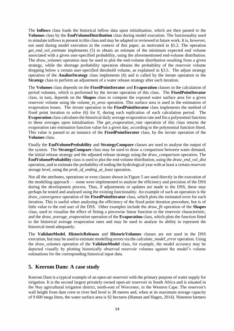
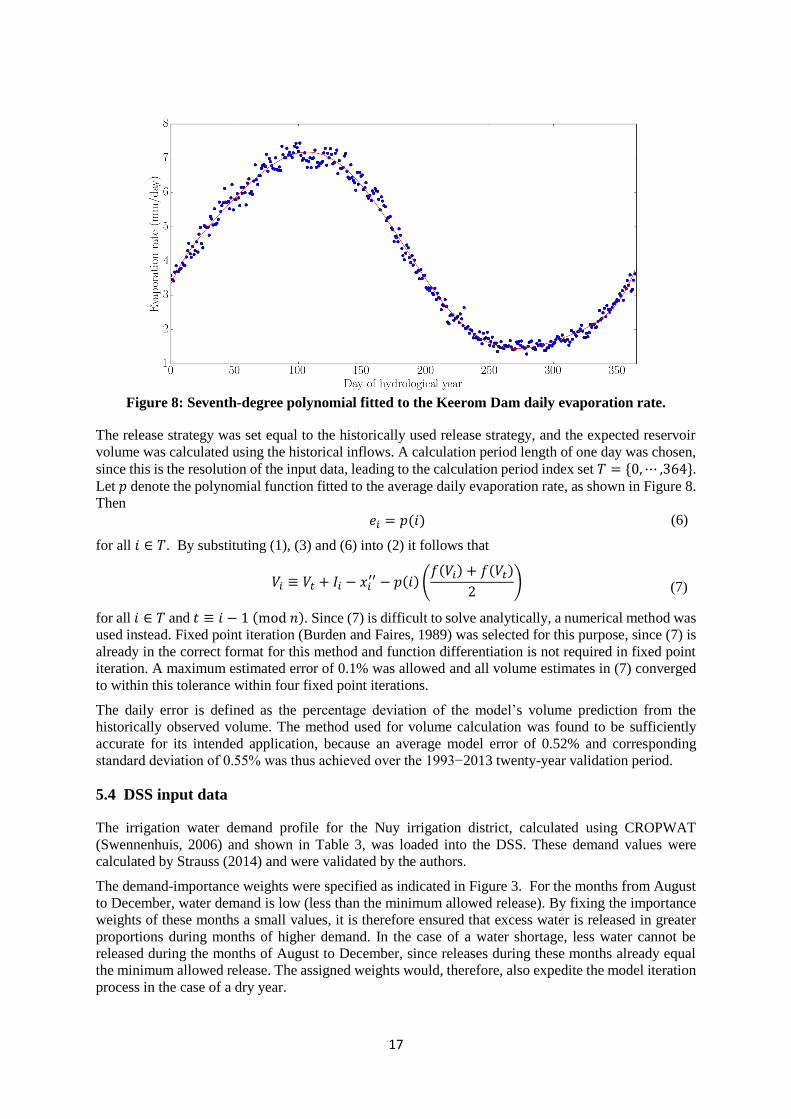
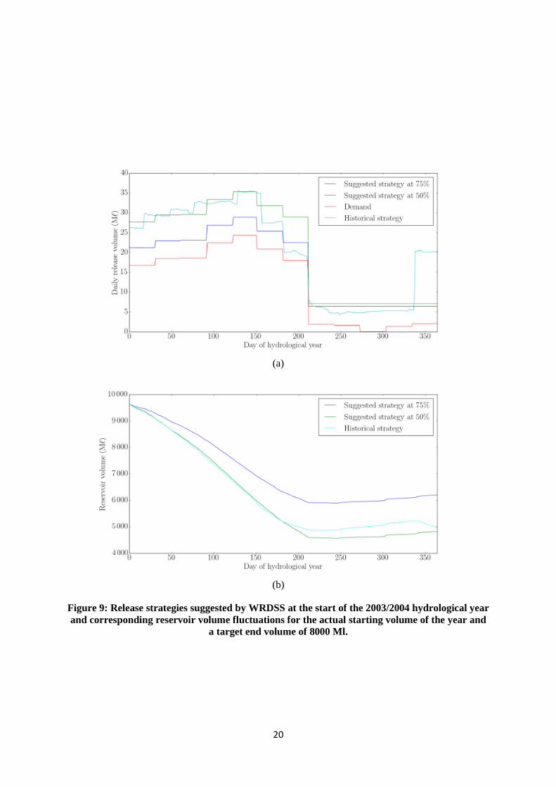
26

Winter T C 1981 Uncertainties in estimating the water balance of lakes JAWRA Journal of the American

Water Resources Association 17(1)82minus115

Yeh WW 1985 Reservoir management and operations models A state-of-the-art review Water Resources

Research 21(12)1797minus1818