decision support for open-air irrigation reservoir control of 450 mm ... open-air reservoirs are...

OperationsResearchSociety ofSouth Africa

Submitted

for publication in

ORiON

OperationsResearch-Society of

South Africa

Decision Support for Open-airIrrigation Reservoir Control

Authors’ identities suppressed: Blind refereeing copy

Abstract

The availability of irrigation water greatly impacts on the profitability of the agriculturalsector in South Africa and is largely determined by prudent decisions related to water re-lease strategies at open-air irrigation reservoirs. The selection of such release strategies isdifficult, since the objectives that should be pursued are not generally agreed upon andunpredictable weather patterns cause reservoir inflows to vary substantially between hy-drological years. In this paper, a decision support system is proposed for the selection ofsuitable water release strategies. The system is based on a mathematical model which gen-erates a probability distribution of the reservoir volume at the end of a hydrological yearbased on historical reservoir inflows. A release strategy is then computed which centres theexpected hydrological year-end reservoir volume on some user-specified target value subjectto user-specified weight factors representing demand satisfaction importance during the var-ious decision periods of the hydrological year. The probability of water shortage for a givenyear-end transition volume may be determined by the DSS, which allows for the computationof acceptable trade-off decisions between the fulfilment of current demand and the futurerepeatability of a release strategy. The system is implemented as a computerised conceptdemonstrator which is validated in a special case study involving Keerom Dam, an open-airreservoir in the Nuy agricultural district near Worcester in the South African Western Cape.The system’s strategy suggestions are compared to historically employed strategies and thesuggested strategies are found to fare better in maintaining reservoir storage levels whilststill fulfilling irrigation demands.

Key words: Decision support, reservoir releases.

1 Introduction

South Africa is classified as a semi-arid, water-stressed region, with an average annualrainfall of 450 mm — almost half the global average of 860 mm [21]. The limited anderratic water supply resulting from precipitation necessitates irrigation in most instancesof crop farming. Open-air reservoirs are most commonly used to store irrigation waterin South Africa, because precipitation periods and river flows are dynamic, in some casesvolatile and not necessarily overlapping with demand periods. There are approximately1.3 million hectares of agricultural land under irrigation in South Africa and agricultureaccounts for roughly fifty percent of South Africa’s total annual water usage [21].

1

2 Authors’ identities suppressed: Blind refereeing copy

If irrigation reservoir levels are not carefully controlled, water shortages or flood damagemay occur downstream from the reservoirs with disastrous effects for farmers in the re-gion. An effective release strategy must therefore be employed for beneficial reservoir levelcontrol. A suitable choice of irrigation reservoir release strategy is, however, not obviousfor a number of reasons. The objectives that should be pursued by such a strategy arenot generally agreed upon. Irrigation demands should obviously be met, while the risk ofwater shortage and/or the risk of flood damage may be minimised, or evaporation lossesmay be minimised. Unpredictable weather patterns furthermore cause reservoir annualinflows to vary substantially, thus making planning and water allocation exceedingly dif-ficult. The determination of irrigation demand is also a non-trivial problem, which isinfluenced by the climate as well as the distribution of crop types under irrigation andvarious agricultural policies. Finally, the decision makers responsible for the selection of arelease strategy may differ vastly in their attitude toward risk, which plays a critical rolein the selection of a consensus strategy.

The problem considered in this paper is the design and implementation of a user-friendly,computerised decision support system (DSS) which may aid the operators of an open-airirrigation reservoir in deciding upon a suitable water release strategy. This DSS provides ameans for the effective comparison of different water release strategies through quantitativeperformance metrics and is also capable of suggesting a strategy which best achieves user-specified levels of these performance metrics. The DSS put forward in this paper relieson a mathematical modelling framework, previously suggested by van der Walt and vanVuuren [24]. This framework accommodates trade-off decisions between the fulfilment ofdemand and future strategy repeatability. These trade-offs are accomplished by balancingthe conflicting objectives of maximising the fulfilment of irrigation demand (and hencereservoir releases), whilst simultaneously minimising the risk of water shortage, withincertain specified legal and environmental constraints.

The paper is organised as follows. A concise review of the literature related to the notionof reservoir release strategy formulation is presented in §2, after which the mathematicalmodelling framework for reservoir releases of van der Walt and van Vuuren [24] is brieflyreviewed in §3. A novel computerised DSS, based on the framework of §3, is described in§4 and then applied in §5 to a special case study involving Keerom Dam, a large open-air irrigation reservoir in the South African Western Cape. The working of the DSS is,however, generic and its potential use at other irrigation reservoirs may hold significantbenefit in view of its successful application in the case of Keerom Dam. The paper finallycloses in §6 with a brief appraisal of the contribution and some ideas with respect topossible follow-up future work.

2 Literature review

In the first section of this literature review, we describe a number of methods availablefor meteorological data prediction, after which the focus turns in §2.2 to approaches avail-able in the literature for calculating irrigation demand. The review closes in §2.3 with adescription of the methods available for evaporation estimation and modelling as well asan overview in §2.4 of DSSs previously established for open-air reservoir control.

Decision Support for Open-air Irrigation Reservoir Control 3

2.1 Meteorological prediction and generation models

Precipitation in the catchment area of a reservoir and the resulting inflows into the reser-voir are the most volatile and unpredictable variables in the reservoir sluice control prob-lem under consideration. While extensive research has been devoted to weather prediction,long-term weather patterns remain largely unpredictable [9]. As a result, weather gener-ators are often used to simulate volatile weather conditions exhibiting seemingly randombehaviour when the effects of weather patterns have to be studied. Most weather genera-tors have been developed for the study of precipitation, because of the far reaching effectsof rainfall on many environmental processes [27].

According to Wilks and Wilby [27], most weather generators are based on the assumptionthat the precipitation volumes on consecutive wet days are independent. The MonteCarlo simulation method, which is often used in such weather generators, consists of usinga pseudo-random number generator in conjunction with a precipitation distribution curve,fitted to historical data, in order to generate random precipitation amounts.

It has, however, been observed that wet and dry days do not occur randomly and inde-pendently, but that they rather tend to cluster together in wet or dry spells [27]. Dryspells cause a discontinuity in the precipitation distribution and thus cannot be modelledadequately using only the procedure described above. The occurrence of a wet or dry spellmay be simulated effectively as a Markov chain. Once the state of a day has been simu-lated (wet or dry), the precipitation amount associated with a wet day may be simulatedusing the Monte Carlo method.

If the flows of a river are to be modelled using the Monte Carlo method, it is unnecessaryto embed a Markov chain in the simulation, however, since there are no correspondingdiscontinuities in the flow distributions. The effects of discontinuous precipitation areinstead absorbed by the gradual water flows in the catchment area and are also lessenedby other sources of water, such as water springs or smaller rivers.

Successful river flow predictions have been achieved by standard time series modelling, asdescribed by Box and Jenkins [2]. Artificial neural networks have also been employed forthis purpose, achieving greater accuracies than time series modelling in some cases [8].

The choice between a generation or prediction approach to reservoir inflows may have asignificant impact on the usefulness of the DSS put forward in this paper. Time series andartificial neural network prediction models rely on the assumption that the immediatefuture behaviour of the system depends more sensitively on recent historical behaviourthan on non-recent historical behaviour. While this may prove true for short-term predic-tions (a small number of days for general weather prediction), it remains inaccurate overannual predictions [9]. Using prediction models in the DSS put forward in this paper maytherefore result in overly optimistic strategy suggestions.

2.2 Irrigation demand calculation

The calculation of crop irrigation demand is an important constituent part of the proposedsolution to the problem under consideration in this paper. It is essential to be ableto forecast irrigation demand, at least annually, for planning purposes. Several factors


may influence the irrigation demand on a farm, depending on the calculation methodused. Irrigation demand may be estimated from an economic point of view, taking intoaccount water cost, crop yields and cost-benefit trade-offs. This approach to derivingirrigation demand may be adopted in conjunction with statistical estimation methods orprogramming models, as described by Bontemps and Couture [1]. The use of statisticalestimation methods for deriving irrigation water demand results in inelastic water demandprofiles. The reason for this may be a lack of data on crop-level water use [1]. Whenusing programming models, however, inelastic demand profiles result only below a certainthreshold water price.

In the DSS proposed here, a fixed (inelastic) demand profile is assumed as input to serveas a fixed reference point for performance measures in the model. This profile serves thedual purpose of being the primary input in the selection of an initial water release strategy(which is improved iteratively by the DSS), and as a measure of how well demand is metby comparing the actual reservoir outflows to this demand profile. Therefore, the demandprofile employed in this study should ideally reflect crop needs, irrespective of water price.It is envisaged that the model developed here may ultimately be used in an economicbenefit study, instead of incorporating the cost-benefit analysis in the demand calculation.

According to Willis and Whittlesey [26], a farmer’s risk nature determines the degree towhich his preferred irrigation policy exceeds the net irrigation requirements of his crops.There is a cost associated with this over-allocation of water, referred to as a self-protectioncost. An analysis of each farmer’s utility function and preferred self-protection cost isbeyond the scope of this paper. Since it is expected that several farmers may benefit fromthe reservoir for which a sluice release strategy is sought, using a method for determiningeach farm’s irrigation requirements, which is standardised and independent of subjectivepreferences, may be beneficial. Such an approach excludes individual risk preference whendetermining the annual water demand profile for a reservoir; it rather depends only oncrop water requirements. This is referred to as the net irrigation requirement.

A globally accepted standard for the calculation of fixed crop water requirements in ir-rigation studies was published by the Food and Agriculture Organisation of the UnitedNations in 1974 [15]. This standard was updated and improved in 1990 by a panel con-sisting of members of the International Commission for Irrigation and Drainage as well asthe World Meteorological Organisation. The resulting current standard is referred to asthe FAO Penman-Monteith method [15].

CROPWAT 8.0 for Windows [19] is a DSS for the calculation of net irrigation requirements,based on soil, climate and crop data. All calculations performed in CROPWAT followthe FAO Penman-Monteith method. The equivalent South African standard is the DSSSAPWAT [23].

2.3 Evaporation estimation and modelling

Evaporation from a water surface is the net rate of water transported from the surface intothe atmosphere [18]. Estimations of evaporation losses are required by all water balancemodels for water reservoir systems. The modelling approach adopted in this paper topredict future evaporation losses is discussed here.


Evaporation losses are usually assumed to be proportional to the average exposed watersurface area [17]. Van Vuuren and Grundlingh [25] modelled evaporation loss during periodi in a set T = {0, . . . , n− 1} of calculation periods spanning a hydrylogical year as

Ei = eiAi +At

2, (1)

where t ≡ i − 1(modn) and Ai denotes the exposed water surface area at the end ofcalculation period i ∈ T . Here ei is the evaporation rate associated with calculationperiod i ∈ T , as determined from historical evaporation rates.

As their aim was to employ (1) in a linear programming model, van Vuuren and Grundlingh[25] assumed a linear relationship between reservoir storage and exposed water surfacearea. The relationship between the exposed water surface area and reservoir storage, asdefined by the local topography, is, however, usually non-linear. Sun et al. [17] developeda piecewise linear model for approximating evaporation losses as a function of reservoirstorage. The latter approach is also adopted in this paper.

2.4 Decision support systems

There exists no universally agreed-upon definition for the notion of a DSS. A range ofdefinitions have been proposed, with the one extreme focussing on the notion of decisionsupport and the other on the notion of a system [10]. Shim et al. [14] state that “DSSsare computer technology solutions that can be used to support complex decision makingand problem solving.” The development of DSSs draws from two main areas of research,namely theoretical studies and organisational decision making [14].

DSSs may be partitioned into the categories of collaborative support systems, optimisation-based decision support models and active decision support [14]. Collaborative supportsystems aid groups of agents engaged in cooperative work by sharing information acrossorganisational, space or time boundaries with the aim of facilitating effective consensusdecision making. Optimisation-based decision support models generally consist of threesequential stages. First, a system is abstractly modelled in such a manner that solutionobjectives can be expressed in a quantitative manner, after which the model is solved ac-cording to some algorithmic approach. Finally, the solution or set of solutions is analysedin terms of their possible effects on the system [14]. The term active decision supportrefers to a DSS’s ability to adapt its output actively when new inputs are entered, asused by van Vuuren and Grundlingh [25], thus contrasting DSSs used mainly for strategicplanning purposes to those which can be used for operational decision making. The DSSproposed in this paper falls in the latter category.

The farmers who benefit from crop irrigation reservoirs are often in agreement that therelease of more water (up to maximum sluice capacity, thus not including floods) is morebeneficial than the release of less water [5]. It may therefore be assumed that the benefitfunction for normal operation of an irrigation reservoir is a strictly increasing function ofrelease volume. This assumption renders the problem of determining a suitable releasestrategy fairly simple: release the maximum amount of water, keeping in mind the risk ofnot being able to achieve repeatability of the strategy over successive hydrological years.The focus of a reservoir release DSS should therefore be on quantifying the risk related


to a given release strategy, rather than merely searching for an optimal strategy or set ofstrategies.

Two DSSs have previously been developed for implementation at Keerom Dam. The firstis ORMADSS, developed by van Vuuren and Grundlingh [25] in 1998. This DSS relies ona linear programming model for determining an optimal release strategy during averageyears with the objective of minimising evaporation losses. The DSS receives the actualreservoir level and other user-defined parameters as inputs and attempts to steer the actualreservoir level to the optimal reservoir level for average years.

ORMADSS was validated using data from the 1990/91 hydrological year, by comparingthe total water yield and evaporation losses corresponding to the historical release strat-egy (based on the benefiting farmers’ intuition) to those of the release strategies suggestedby ORMADSS. The overly conservative nature of the farmers became apparent duringthe validation process, with the suggested strategies outperforming the historically imple-mented strategy for 0%, 20%, and 40% reservoir reserve levels. The DSS was taken in usein 2000, but after extremely dry years in 2002 and 2003, where the reservoir level fell tobelow 25% of its capacity, confidence in the DSS decreased and it fell out of use.

Strauss [16] then attempted in 2014 to improve upon this DSS by adapting the way inwhich risk is accommodated. In addition to a minimum reserve for the operating level ofthe reservoir, Strauss implemented risk-related constraints in the form of release quantityupper and lower bounds in the underlying mathematical model. This adaptation does not,however, quantify risk explicitly, and therefore does not provide greater security in termsof the risk of non-repeatability of the suggested strategy. Since no quantitative measureof risk related to a given strategy is available, users cannot ascertain the extent to whichthey are exposing themselves to the possibility of future water shortages if they choose tofollow the suggested strategy. It may follow that a decision maker who was reluctant tocontinue using ORMADSS will view this adaptation in the same regard. The latter DSShas not, in fact, been taken in use.

Strauss [16] criticised the simplistic manner in which van Vuuren and Grundlingh [25] ac-commodated risk by only including a minimum reserve for the operating level of the reser-voir, while not directly allowing for the possibility of unmet demand. Strauss neverthelessimplemented a very similar model, together with the additional risk-related constraints inthe form of release quantity upper and lower bounds. It is important to note, however,that risk was also not quantified explicitly in the model of Strauss [16].

Having access to a quantitative representation of risk is a crucial element lacking in the twoDSSs reviewed above. Furthermore, models which provide a single optimal solution maybe insufficient, since reservoir operation commonly involves trade-off decision options. Inresponse, multi-objective models have often been implemented in the context of reservoirmanagement.

3 Mathematical modelling framework

In this section, the 2015 mathematical modelling framework for reservoir releases of vander Walt and van Vuuren [24] is briefly reviewed. This framework attempts to balance the


conflicting objectives of water demand fulfilment and future water shortage risk, takinginto account certain user preferences. The framework facilitates a comparison of differentrelease strategies in terms of a trade-off between various quantitative performance metrics.

3.1 Modelling assumptions

In order to develop a mathematical modelling framework for irrigation reservoir operation,van der Walt and van Vuuren [24] made a number of important modelling assumptions.They discretised the scheduling horizon over which a release strategy is to be determinedinto a number of time intervals, called calculation periods, which are typically days orweeks. Their model is therefore discrete in nature. The minimum possible duration overwhich a constant water release rate can be implemented, as determined by the frequencywith which sluice adjustments are allowed, is called the decision period length. Decisionperiods are typically weeks, fortnights or months, but their length is in any case a multipleof the calculation period length. Water demand during a specific decision period was alsoassumed to be constant, which is an acceptable assumption for short decision periods.

Van der Walt and van Vuuren [24] furthermore assumed that the evaporation rate expe-rienced at the reservoir during a given calculation period is directly proportional to theaverage exposed water surface area of the reservoir and thus a function of the averagereservoir volume during that period, according to (1). The coefficient of proportionality eiin (1) was taken to depend on the historical meteorological conditions of the time intervalin question. The South African Department of Water Affairs and Forestry [6] maintainsa database of all reservoirs exceeding a certain minimum storage capacity, which includeshistorical daily evaporation losses for these reservoirs. These loss rates may be used toestimate the coefficient ei in (1) for all i ∈ T . For new reservoirs, the evaporation rates ofolder reservoirs in the vicinity may be used as an initial estimate.

The repeatability of any reservoir release strategy is taken to depend on an estimate ofthe most likely reservoir volume at the end of the hydrological year as a result of thisstrategy. In particular, van der Walt and van Vuuren [24] took the reservoir volumeduring the transition between two consecutive hydrological years as a measure of futuredemand fulfilment security. A hydrological year in South Africa runs from October 1st toSeptember 30th.

Van der Walt and van Vuuren [24] finally adopted a standard conservation law in theform of the assumption that the change in water volume during a given calculation periodequals the net influx (including all the reservoir’s water sources, precipitation onto thereservoir and in its catchment area, as well as seepage losses), less evaporation losses andall reservoir outflows, including controlled sluice outflow and overflow.

3.2 Modelling framework for reservoir releases

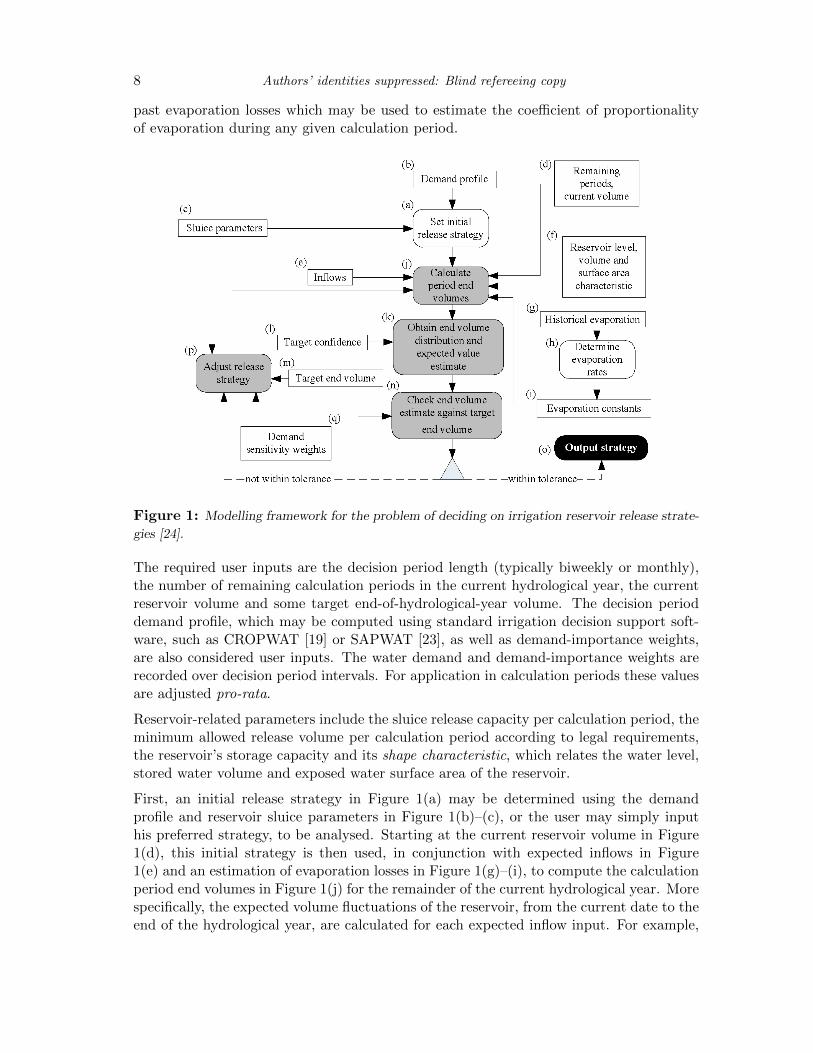
The conceptual mathematical modelling framework of van der Walt and van Vuuren [24]is illustrated graphically in Figure 1. In this framework, the model inputs have been parti-tioned into historical data, as well as various user-inputs and reservoir-related parameters.Historical data refer to past inflows, used as an indication of possible future inflows, and


past evaporation losses which may be used to estimate the coefficient of proportionalityof evaporation during any given calculation period.

Figure 1: Modelling framework for the problem of deciding on irrigation reservoir release strate-

gies [24].

The required user inputs are the decision period length (typically biweekly or monthly),the number of remaining calculation periods in the current hydrological year, the currentreservoir volume and some target end-of-hydrological-year volume. The decision perioddemand profile, which may be computed using standard irrigation decision support soft-ware, such as CROPWAT [19] or SAPWAT [23], as well as demand-importance weights,are also considered user inputs. The water demand and demand-importance weights arerecorded over decision period intervals. For application in calculation periods these valuesare adjusted pro-rata.

Reservoir-related parameters include the sluice release capacity per calculation period, theminimum allowed release volume per calculation period according to legal requirements,the reservoir’s storage capacity and its shape characteristic, which relates the water level,stored water volume and exposed water surface area of the reservoir.

First, an initial release strategy in Figure 1(a) may be determined using the demandprofile and reservoir sluice parameters in Figure 1(b)–(c), or the user may simply inputhis preferred strategy, to be analysed. Starting at the current reservoir volume in Figure1(d), this initial strategy is then used, in conjunction with expected inflows in Figure1(e) and an estimation of evaporation losses in Figure 1(g)–(i), to compute the calculationperiod end volumes in Figure 1(j) for the remainder of the current hydrological year. Morespecifically, the expected volume fluctuations of the reservoir, from the current date to theend of the hydrological year, are calculated for each expected inflow input. For example,


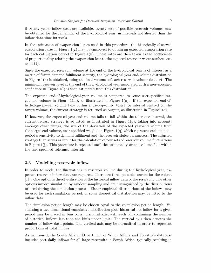
if twenty years’ inflow data are available, twenty sets of possible reservoir volumes maybe obtained for the remainder of the hydrological year, in intervals not shorter than theinflow data time intervals.

In the estimation of evaporation losses used in this procedure, the historically observedevaporation rates in Figure 1(g) may be employed to obtain an expected evaporation ratefor each calculation period in Figure 1(h). These rates are then taken as the coefficientsof proportionality relating the evaporation loss to the exposed reservoir water surface areaas in (1).

Since the expected reservoir volume at the end of the hydrological year is of interest as ametric of future demand fulfilment security, the hydrological year end-volume distributionin Figure 1(k) is obtained, using the final volumes of each reservoir volume data set. Theminimum reservoir level at the end of the hydrological year associated with a user-specifiedconfidence in Figure 1(l) is then estimated from this distribution.

The expected end-of-hydrological-year volume is compared to some user-specified tar-get end volume in Figure 1(m), as illustrated in Figure 1(n). If the expected end-of-hydrological-year volume falls within a user-specified tolerance interval centred on thetarget volume, the current strategy is returned as output, as illustrated in Figure 1(o).

If, however, the expected year-end volume fails to fall within the tolerance interval, thecurrent release strategy is adjusted, as illustrated in Figure 1(p), taking into account,amongst other things, the size of the deviation of the expected year-end volume fromthe target end volume, user-specified weights in Figure 1(q) which represent each demandperiod’s sensitivity to demand fulfilment and the reservoir sluice parameters. The adjustedstrategy then serves as input for the calculation of new sets of reservoir volume fluctuationsin Figure 1(j). This procedure is repeated until the estimated year-end volume falls withinthe user specified tolerance interval.

3.3 Modelling reservoir inflows

In order to model the fluctuations in reservoir volume during the hydrological year, ex-pected reservoir inflow data are required. There are three possible sources for these data[11]. One option is direct utilisation of the historical inflow data of the reservoir. The otheroptions involve simulation by random sampling and are distinguished by the distributionsutilised during the simulation process. Either empirical distributions of the inflows maybe used for each simulation period, or some theoretical distribution may be fitted to theinflow data.

The simulation period length may be chosen equal to the calculation period length. Vi-sualising a two-dimensional cumulative distribution plot, historical net inflow for a givenperiod may be placed in bins on a horizontal axis, with each bin containing the numberof historical inflows less than the bin’s upper limit. The vertical axis then denotes thenumber of inflow data points. The vertical axis may be normalised in order to representproportions of total inflows.

As mentioned, the South African Department of Water Affairs and Forestry’s databaseincludes past daily inflows for all large reservoirs in South Africa, typically resulting in


ample historical inflow data. This allows for the determination of accurate reservoir inflowdistributions. In other words, it is usually not necessary to fit a theoretical distributionto the data — the empirically obtained distributions may instead be utilised directly. Fora newly built reservoir, the prediction of future inflows in the absence of historical datawould constitute a challenging, separate research project.

Utilising the inflow distributions described above, inflows may be emulated by Monte Carlosimulation. Let Ii be the net reservoir inflow during simulation period i ∈ T and let Ube a uniform random variable on the interval [0, 1]. If Ii has the cumulative distributionfunction Fi, then F−1i (U) has the same distribution as Ii. An instance of Ii may thereforebe simulated according to the inverse transform method [12] by generating a uniform [0, 1]variate u and recording the value F−1i (u). Once this has been done for each simulationperiod, the inflows of a single hydrological year have been simulated. A large number ofhypothetical parallel years may thus be simulated.

In the simulation approach described above, it is assumed that inflows during adjacentsimulation periods are independent. The validity of this assumption may be tested bycomparing selected statistical properties of inflows thus simulated to those of the histor-ically observed inflows. A simulation approach with the incorporation of memory, suchas an artificial neural network or a modified Markov chain, would not rely on the afore-mentioned assumption. Such approaches would, however, include a degree of prediction,as mentioned in §2.1, which may result in overly optimistic planning. In fact, given theextremely volatile nature of weather patterns, any attempt at synthetically increasing theinformation inherent in historical inflow data over long planning horizons (such as oneyear, for example) may result in an unsubstantiated increase in knowledge related to thebehaviour of inflows.

3.4 Estimating period end-volume distributions

Let Vi denote the reservoir volume at the end of calculation period i, let xi be the watervolume released during calculation period i, and let Ei be the volume of water lost dueto evaporation during calculation period i, where i ∈ T , for some set T = {0, . . . , n −1} of calculation periods spanning a hydrological year. Furthermore, let ei denote theevaporation rate per unit of average exposed water surface area during calculation periodi ∈ T , denoted by Ai. Then it follows that

Vi = Vt + Ii − xi − Ei (2)

for all i ∈ T and t ≡ i − 1 (modn), into which expression (1) may be substituted. Fur-thermore, the exposed surface area of the reservoir in (1) is related to the stored watervolume according to some reservoir shape characteristic f in the sense that

Ai = f(Vi) (3)

for all i ∈ T . A preliminary release strategy is determined according to the water demandprofile and the sluice release parameters. Let Di denote the water demand during calcula-tion period i ∈ T , and let xmin and xmax denote respectively the minimum and maximum


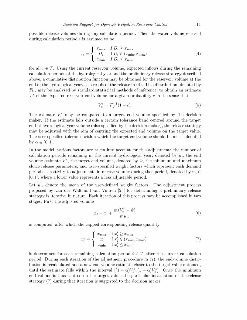
possible release volumes during any calculation period. Then the water volume releasedduring calculation period i is assumed to be

xi =

xmax if Di ≥ xmax

Di if Di ∈ (xmin, xmax)xmin if Di ≤ xmin

(4)

for all i ∈ T . Using the current reservoir volume, expected inflows during the remainingcalculation periods of the hydrological year and the preliminary release strategy describedabove, a cumulative distribution function may be obtained for the reservoir volume at theend of the hydrological year, as a result of the release in (4). This distribution, denoted byFV , may be analysed by standard statistical methods of inference, to obtain an estimateV ∗c of the expected reservoir end volume for a given probability c in the sense that

V ∗c = F−1V (1− c). (5)

The estimate V ∗c may be compared to a target end volume specified by the decisionmaker. If the estimate falls outside a certain tolerance band centred around the targetend-of-hydrological year volume (also specified by the decision maker), the release strategymay be adjusted with the aim of centring the expected end volume on the target value.The user-specified tolerance within which the target end volume should be met is denotedby α ∈ (0, 1].

In the model, various factors are taken into account for this adjustment: the number ofcalculation periods remaining in the current hydrological year, denoted by m, the endvolume estimate V ∗c , the target end volume, denoted by Φ, the minimum and maximumsluice release parameters, and user-specified weight factors which represent each demandperiod’s sensitivity to adjustments in release volume during that period, denoted by wi ∈[0, 1], where a lower value represents a less adjustable period.

Let µw denote the mean of the user-defined weight factors. The adjustment processproposed by van der Walt and van Vuuren [25] for determining a preliminary releasestrategy is iterative in nature. Each iteration of this process may be accomplished in twostages. First the adjusted volume

x′i = xi +wi(V

∗c − Φ)

mµw(6)

is computed, after which the capped corresponding release quantity

x′′i =

xmax if x′i ≥ xmax

x′i if x′i ∈ (xmin, xmax)xmin if x′i ≤ xmin

(7)

is determined for each remaining calculation period i ∈ T after the current calculationperiod. During each iteration of the adjustment procedure in (7), the end-volume distri-bution is recalculated and a new end-volume estimate closer to the target value obtained,until the estimate falls within the interval [(1 − α)V ∗c , (1 + α)V ∗c ]. Once the minimumend volume is thus centred on the target value, the particular incarnation of the releasestrategy (7) during that iteration is suggested to the decision maker.


3.5 Quantifying the risk of water shortage

As mentioned, the repeatability of a release strategy is taken to depend on the reservoirvolume during the transition between two successive hydrological years as a result ofapplying the strategy. The probability of water shortage associated with a reservoir volumeduring this transition may be determined by equating the starting and target end volumesin the model, and solving the model for a given probability level. The number of timesthat the reservoir volume drops below a user-specified threshold volume and the lengthof time the volume remains below this threshold, for all historically observed inflows,may be taken as an estimate of the probability of water shortage associated with a givenrelease strategy, transition volume and probability level. This probability estimate maybe adopted as a performance metric when comparing release strategies.

During any period in an actual year, the probability of reaching the end of the hydrolog-ical year with at least a certain reservoir volume may be obtained from the end-volumeprobability distribution resulting from the current release strategy. Either the probabilityof obtaining a certain minimum end volume, or the minimum end volume expected tobe obtained for a fixed probability, may thus be adopted as a second performance metricwhen comparing release strategies.

In the case of a particularly dry year, when the notion of risk requires special attention,trade-off decisions between the fulfilment of the current hydrological year’s demand andfuture repeatability associated with the release strategy may be required. Future repeata-bility here refers to a level of confidence in the ability to fulfil the irrigation demandsof subsequent years. Due to particularly low reservoir storage levels during a dry year,the decision maker may prefer to aim for a lower target end volume, since the proposedstrategy which centres the end-volume distribution on the specified target value for re-peatability to within the acceptable tolerance interval fails to meet the current year’sdemand adequately. The fulfilment of the current hydrological year’s demand will therebybe improved, but at the cost of a decrease in the security of future years’ water supply.The improvement in demand fulfilment, as well as the decrease in security, may finally bequantified and compared in terms of benefit and cost trade-offs.

4 Decision support system

The design and implementation of a novel DSS concept demonstrator, based on the math-ematical modelling framework of §3, is described in this section. Section 4.1 is devoted toa description of the working of the concept demonstrator graphical user interface, whilethe method of implementation of this concept demonstrator is described in §4.2.

4.1 Working of the concept demonstrator

In order to validate the modelling framework of §3, a concept demonstrator of the frame-work was implemented in Python 2.7 on a personal computer. This DSS is referred toas WRDSS — an acronym for Water Reservoir Decision Support System. The user maylink WRDSS to a specific irrigation reservoir by providing its historical inflow profileI0, . . . , In−1, the historical evaporation rates e0, . . . , en−1 experienced at the reservoir, the


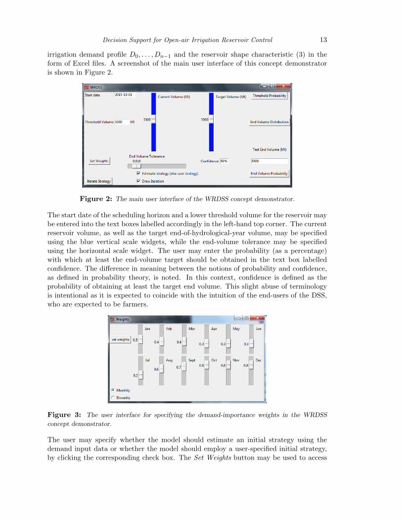
irrigation demand profile D0, . . . , Dn−1 and the reservoir shape characteristic (3) in theform of Excel files. A screenshot of the main user interface of this concept demonstratoris shown in Figure 2.

Figure 2: The main user interface of the WRDSS concept demonstrator.

The start date of the scheduling horizon and a lower threshold volume for the reservoir maybe entered into the text boxes labelled accordingly in the left-hand top corner. The currentreservoir volume, as well as the target end-of-hydrological-year volume, may be specifiedusing the blue vertical scale widgets, while the end-volume tolerance may be specifiedusing the horizontal scale widget. The user may enter the probability (as a percentage)with which at least the end-volume target should be obtained in the text box labelledconfidence. The difference in meaning between the notions of probability and confidence,as defined in probability theory, is noted. In this context, confidence is defined as theprobability of obtaining at least the target end volume. This slight abuse of terminologyis intentional as it is expected to coincide with the intuition of the end-users of the DSS,who are expected to be farmers.

Figure 3: The user interface for specifying the demand-importance weights in the WRDSS

concept demonstrator.

The user may specify whether the model should estimate an initial strategy using thedemand input data or whether the model should employ a user-specified initial strategy,by clicking the corresponding check box. The Set Weights button may be used to access


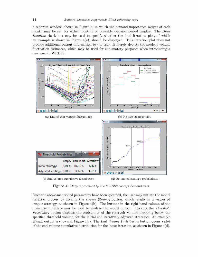
a separate window, shown in Figure 3, in which the demand-importance weight of eachmonth may be set, for either monthly or biweekly decision period lengths. The DrawIteration check box may be used to specify whether the final iteration plot, of whichan example is shown in Figure 4(a), should be displayed. This iteration plot does notprovide additional output information to the user. It merely depicts the model’s volumefluctuation estimates, which may be used for explanatory purposes when introducing anew user to WRDSS.

(a) End-of-year volume fluctuations (b) Release strategy plot

(c) End-volume cumulative distribution (d) Estimated strategy probabilities

Figure 4: Output produced by the WRDSS concept demonstrator.

Once the above-mentioned parameters have been specified, the user may initiate the modeliteration process by clicking the Iterate Strategy button, which results in a suggestedoutput strategy, as shown in Figure 4(b). The buttons in the right-hand column of themain user interface may be used to analyse the model output. Clicking the ThresholdProbability button displays the probability of the reservoir volume dropping below thespecified threshold volume, for the initial and iteratively adjusted strategies. An exampleof such output is shown in Figure 4(c). The End Volume Distribution button opens a plotof the end-volume cumulative distribution for the latest iteration, as shown in Figure 4(d).


The probability of obtaining at least a given end volume may be obtained by entering avolume into the text box labelled Test End Volume (M`) and clicking the End VolumeProbability button. The probabilities of obtaining 5 000 M` or 7 000 M` are, for example,shown in Figure 4(d).

4.2 Implementation of the concept demonstrator

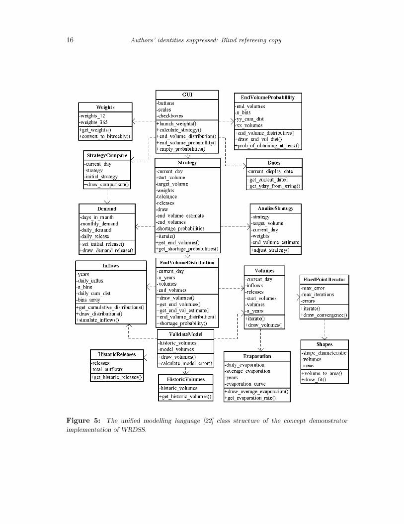
The unified modelling language [22] class structure of the concept demonstrator imple-mentation of WRDSS is shown in Figure 5. In the figure, each class is represented as arectangle, listing its attributes followed by its operations, with the exception of the GUIclass (its attributes have been summarised for the sake of brevity). The attributes of agiven class are the variables which exist in an instance of the class, whilst operations arethe methods which may be performed on these attributes. If one class utilises another atsome point in time, the first class is said to depend on the latter. Class dependency isindicated by dashed arrows in the figure.

The GUI class displays the graphical user interface which creates an instance of theWeights class. This class is used when the user specifies the sensitivity of each demandperiod. By default, constant weight values are stored for each month of the hydrologicalyear, but the convert to biweekly operation is called if the user checks the correspondingradio button, after which the weights are stored in constant biweekly periods by calculatingthe weighted average importance values on a biweekly basis. The Dates class is used toload the current date and manage the start date of the model. The GUI class depends onthe Strategy class for model execution once the user parameters have been specified. TheStrategy class performs the iterative procedure of the mathematical modelling framework,as described in §3.4, and depends on several other classes for its operation. First, theset initial release operation of the Demand class is used to specify the initial releasestrategy. The EndVolumeDistribution class depends on the Volumes and Inflowsclasses. It is used to determine the end-volume distribution resulting from a given releasestrategy by means of the end volume distribution operation.

The Inflows class loads the historical inflow data upon initialisation, which are then passedto the Volumes class by the EndVolumeDistribution class during model execution.The functionality adopted to simulate inflows is present in this class and may be adaptedor reviewed in future work. It is, however, not used during model execution in the contextof this paper, as motivated in the case study to follow. The operation get end vol estimateimplements (5) to obtain an estimate of the expected end volume associated with a givenuser-specified probability according to the aforementioned end-volume distribution. Thedraw volumes operation may be used to plot the end-volume distribution resulting froma given strategy, while the shortage probability operation obtains the probability of thereservoir volume dropping below a certain user-specified threshold volume, as explained in§3.5. The adjust strategy operation of the AnaliseStrategy class implements (7) and iscalled by the iterate operation in the Strategy class to perform an adjustment of a waterrelease strategy after each iteration.

The Volumes class depends on the FixedPointIterator and Evaporation classes inthe calculation of period volumes, which is performed by the iterate operation of this class.The FixedPointIterator class, in turn, depends on the Shapes class to compute the


Figure 5: The unified modelling language [22] class structure of the concept demonstrator

implementation of WRDSS.


exposed water surface area for a given reservoir volume using the volume to area operation.This surface area is employed in the estimation of evaporation losses. The iterate operationin the FixedPointIterator class implements the method of fixed point iteration to solve(2) for Vi during each replication of each calculation period. The Evaporation classcalculates the historical daily average evaporation rate and fits a polynomial function tothese averages upon initialisation. The get evaporation rate operation of this class returnsthe evaporation rate estimation function value for a given day, according to the polynomialfunction fitted. This value is passed to an instance of the FixedPointIterator class, bythe iterate operation of the Volumes class.

Finally, the EndVolumeProbability and StrategyCompare classes facilitate analysisof the system output. The StrategyCompare class may be used to draw a comparisonbetween water demand, the initial release strategy and the adjusted release strategy bymeans of the draw comparison operation. The EndVolumeProbability class is used toplot the end-volume distribution, using the draw end vol dist operation, and to estimatethe probability of ending the hydrological year with at least a certain reservoir storagelevel, using the prob of ending at least operation.

Not all the attributes, operations or even classes shown in Figure 5 are employed directlyin the execution of the modelling approach — some were implemented to analyse theefficiency and precision of the DSS during the development process. Thus, if adjustmentsor updates are made to the DSS, these may perhaps be tested and analysed using theexisting functionality. An example of such an operation is the draw convergence operationof the FixedPointIterator class, which plots the estimated error for each iteration. Thisis useful when analysing the efficiency of the fixed point iteration procedure, but is oflittle value to the end user of the DSS. Other examples include the draw fit operation ofthe Shapes class, used to visualise the effect of fitting a piecewise linear function to thereservoir characteristic, and the draw average evaporation operation of the Evaporationclass, which plots the function fitted to the historical average evaporation rates and maybe used to analyse its ability to represent the historical trend adequately.

The ValidateModel, HistoricReleases and HistoricVolumes classes are not employedin the DSS execution, but may be used to estimate modelling errors via the calculate modelerror operation. Using the draw volumes operation of the ValidateModel class, forexample, the model accuracy may be depicted visually by plotting historically observedreservoir volumes against the model’s volume estimations for the corresponding historicalinput data.

5 Keerom Dam: A case study

Keerom Dam is a typical example of an open-air reservoir with the primary purpose ofwater supply for irrigation. It is the second largest privately owned open-air reservoirin South Africa and is situated in the Nuy agricultural irrigation district, north-east ofWorcester, in the Western Cape. The reservoir’s wall height from dam crest to river bedlevel is 38 metres (m) and, when at its maximum storage capacity of 9 600 mega litres(M`), the water surface area is 92 hectares (ha) [7].


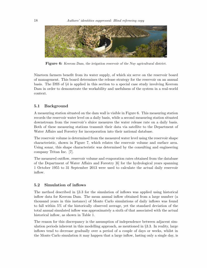
Figure 6: Keerom Dam, the irrigation reservoir of the Nuy agricultural district.

Nineteen farmers benefit from its water supply, of which six serve on the reservoir boardof management. This board determines the release strategy for the reservoir on an annualbasis. The DSS of §4 is applied in this section to a special case study involving KeeromDam in order to demonstrate the workability and usefulness of the system in a real-worldcontext.

5.1 Background

A measuring station situated on the dam wall is visible in Figure 6. This measuring stationrecords the reservoir water level on a daily basis, while a second measuring station situateddownstream from the reservoir’s sluice measures the water release rate on a daily basis.Both of these measuring stations transmit their data via satellite to the Department ofWater Affairs and Forestry for incorporation into their national database.

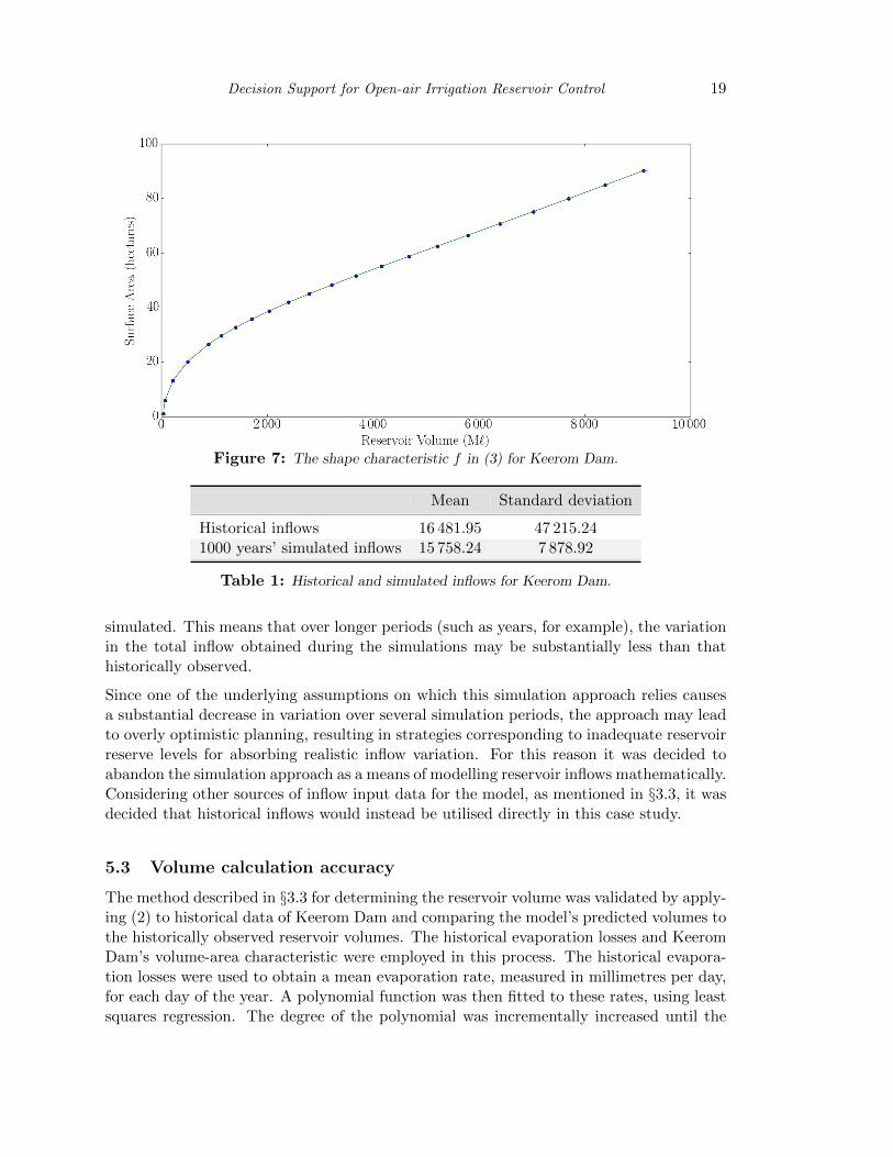
The reservoir volume is determined from the measured water level using the reservoir shapecharacteristic, shown in Figure 7, which relates the reservoir volume and surface area.Using sonar, this shape characteristic was determined by the consulting and engineeringcompany Tritan Inc. [7].

The measured outflow, reservoir volume and evaporation rates obtained from the databaseof the Department of Water Affairs and Forestry [6] for the hydrological years spanning1 October 1955 to 31 September 2013 were used to calculate the actual daily reservoirinflow.

5.2 Simulation of inflows

The method described in §3.3 for the simulation of inflows was applied using historicalinflow data for Keerom Dam. The mean annual inflow obtained from a large number (athousand years in this instance) of Monte Carlo simulations of daily inflows was foundto fall within 5% of the historically observed average, yet the standard deviation of thetotal annual simulated inflow was approximately a sixth of that associated with the actualhistorical inflow, as shown in Table 1.

The reason for this discrepancy is the assumption of independence between adjacent sim-ulation periods inherent in this modelling approach, as mentioned in §3.3. In reality, largeinflows tend to decrease gradually over a period of a couple of days or weeks, whilst inthe Monte Carlo simulation it may happen that a large inflow, lasting only a single day, is


Figure 7: The shape characteristic f in (3) for Keerom Dam.

Mean Standard deviation

Historical inflows 16 481.95 47 215.241000 years’ simulated inflows 15 758.24 7 878.92

Table 1: Historical and simulated inflows for Keerom Dam.

simulated. This means that over longer periods (such as years, for example), the variationin the total inflow obtained during the simulations may be substantially less than thathistorically observed.

Since one of the underlying assumptions on which this simulation approach relies causesa substantial decrease in variation over several simulation periods, the approach may leadto overly optimistic planning, resulting in strategies corresponding to inadequate reservoirreserve levels for absorbing realistic inflow variation. For this reason it was decided toabandon the simulation approach as a means of modelling reservoir inflows mathematically.Considering other sources of inflow input data for the model, as mentioned in §3.3, it wasdecided that historical inflows would instead be utilised directly in this case study.

5.3 Volume calculation accuracy

The method described in §3.3 for determining the reservoir volume was validated by apply-ing (2) to historical data of Keerom Dam and comparing the model’s predicted volumes tothe historically observed reservoir volumes. The historical evaporation losses and KeeromDam’s volume-area characteristic were employed in this process. The historical evapora-tion losses were used to obtain a mean evaporation rate, measured in millimetres per day,for each day of the year. A polynomial function was then fitted to these rates, using leastsquares regression. The degree of the polynomial was incrementally increased until the


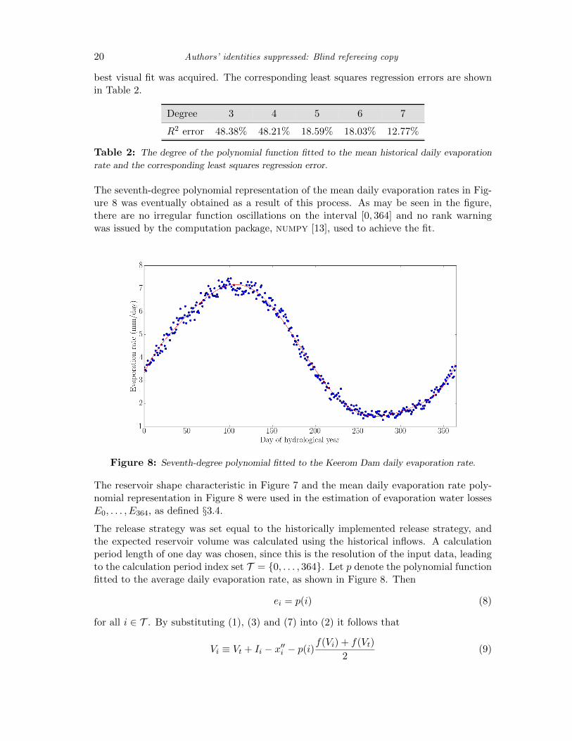
best visual fit was acquired. The corresponding least squares regression errors are shownin Table 2.

Degree 3 4 5 6 7

R2 error 48.38% 48.21% 18.59% 18.03% 12.77%

Table 2: The degree of the polynomial function fitted to the mean historical daily evaporation

rate and the corresponding least squares regression error.

The seventh-degree polynomial representation of the mean daily evaporation rates in Fig-ure 8 was eventually obtained as a result of this process. As may be seen in the figure,there are no irregular function oscillations on the interval [0, 364] and no rank warningwas issued by the computation package, numpy [13], used to achieve the fit.

Figure 8: Seventh-degree polynomial fitted to the Keerom Dam daily evaporation rate.

The reservoir shape characteristic in Figure 7 and the mean daily evaporation rate poly-nomial representation in Figure 8 were used in the estimation of evaporation water lossesE0, . . . , E364, as defined §3.4.

The release strategy was set equal to the historically implemented release strategy, andthe expected reservoir volume was calculated using the historical inflows. A calculationperiod length of one day was chosen, since this is the resolution of the input data, leadingto the calculation period index set T = {0, . . . , 364}. Let p denote the polynomial functionfitted to the average daily evaporation rate, as shown in Figure 8. Then

ei = p(i) (8)

for all i ∈ T . By substituting (1), (3) and (7) into (2) it follows that

Vi ≡ Vt + Ii − x′′i − p(i)f(Vi) + f(Vt)

2(9)


for all i ∈ T and t ≡ i− 1 (modn). Since (9) is difficult to solve analytically, a numericalmethod was used instead. The method of fixed point iteration [3] was selected for this pur-pose, since (9) is already in the correct format for this method and function differentiationis not required in fixed point iteration. A maximum estimated error of 0.1% was allowedand all volume estimates in (9) converged to within this tolerance within four iterations.

The daily volume error is defined as the percentage deviation of the model’s volume pre-diction from the historically observed volume. The method used for volume calculationwas found to be sufficiently accurate for its intended application, because an average dailyvolume error of 0.52% and corresponding standard deviation of 0.55% was thus achievedover the twenty-year validation period 1993–2013.

5.4 DSS input data

The irrigation water demand profile for the Nuy irrigation district, calculated using CROP-WAT [19] and shown in Table 3, was loaded into the DSS. These demand values werecalculated by Strauss [16] and were validated by the authors.

The demand-importance weights were specified as indicated in Figure 3. For the monthsfrom August to December, water demand is low (less than the minimum allowed release).By fixing the importance weights of these months at small values, it is therefore ensuredthat excess water is released in greater proportions during months of higher demand. Inthe case of a water shortage, less water cannot be released during the months of August toDecember, since releases during these months already equal the minimum allowed release.The assigned weights would, therefore, also expedite the model iteration process in thecase of a dry year.

Table Wine Vege-grapes grapes Orchards Olives tables Cereals Lucerne Total

Oct 0.82 154.63 13.34 80.48 8.11 31.89 229.00 518.27Nov 2.54 158.59 13.68 103.18 8.32 32.71 234.87 553.89Dec 3.93 163.64 17.37 106.47 8.58 33.75 242.34 576.08Jan 5.39 220.58 17.08 131.56 9.64 37.92 272.23 694.40Feb 5.18 194.27 18.05 126.40 10.19 40.07 287.71 681.87Mar 4.14 193.91 10.29 100.93 10.17 40.00 287.18 646.62Apr 2.25 168.68 8.96 65.85 8.85 34.79 249.82 539.20May 0.78 0.00 0.00 56.84 0.00 0.00 0.00 57.62Jun 0.00 0.00 0.00 48.97 0.00 0.00 0.00 48.97Jul 0.00 0.00 0.00 0.00 0.00 0.00 0.00 0.00Aug 0.00 0.00 4.66 38.11 0.00 0.00 0.00 42.77Sep 0.71 0.00 7.12 52.34 0.00 0.00 0.00 60.17

Total 25.74 1 254.30 110.55 911.13 63.86 251.13 1 803.15 4 419.86

Table 3: Irrigation demand of the Nuy agricultural district in M` [16].


5.5 Transition volume analysis

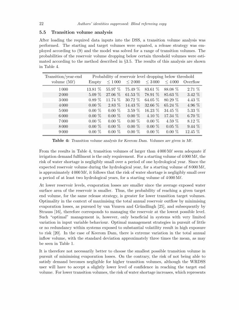
After loading the required data inputs into the DSS, a transition volume analysis wasperformed. The starting and target volumes were equated, a release strategy was em-ployed according to (9) and the model was solved for a range of transition volumes. Theprobabilities of the reservoir volume dropping below certain threshold volumes were esti-mated according to the method described in §3.5. The results of this analysis are shownin Table 4.

Transition/year-end Probability of reservoir level dropping below thresholdvolume (M`) Empty ≤ 1 000 ≤ 2 000 ≤ 3 000 ≤ 4 000 Overflow

1 000 13.81 % 55.97 % 75.49 % 83.61 % 88.08 % 2.71 %2 000 5.09 % 27.06 % 61.53 % 78.91 % 85.63 % 3.42 %3 000 0.89 % 11.74 % 30.72 % 64.05 % 80.29 % 4.43 %4 000 0.00 % 2.83 % 14.43 % 32.66 % 65.24 % 4.96 %5 000 0.00 % 0.00 % 3.59 % 16.23 % 34.45 % 5.33 %6 000 0.00 % 0.00 % 0.00 % 4.10 % 17.34 % 6.70 %7 000 0.00 % 0.00 % 0.00 % 0.00 % 4.59 % 8.12 %8 000 0.00 % 0.00 % 0.00 % 0.00 % 0.05 % 9.44 %9 000 0.00 % 0.00 % 0.00 % 0.00 % 0.00 % 12.45 %

Table 4: Transition volume analysis for Keerom Dam. Volumes are given in M`.

From the results in Table 4, transition volumes of larger than 4 000 M` seem adequate ifirrigation demand fulfilment is the only requirement. For a starting volume of 4 000 M`, therisk of water shortage is negligibly small over a period of one hydrological year. Since theexpected reservoir volume during the hydrological year, for a starting volume of 8 000 M`,is approximately 4 000 M`, it follows that the risk of water shortage is negligibly small overa period of at least two hydrological years, for a starting volume of 4 000 M`.

At lower reservoir levels, evaporation losses are smaller since the average exposed watersurface area of the reservoir is smaller. Thus, the probability of reaching a given targetend volume, for the same release strategy, is greater for lower transition target volumes.Optimality in the context of maximising the total annual reservoir outflow by minimisingevaporation losses, as pursued by van Vuuren and Grundlingh [25], and subsequently byStrauss [16], therefore corresponds to managing the reservoir at the lowest possible level.Such “optimal” management is, however, only beneficial in systems with very limitedvariation in input variable behaviour. Optimal management strategies in pursuit of littleor no redundancy within systems exposed to substantial volatility result in high exposureto risk [20]. In the case of Keerom Dam, there is extreme variation in the total annualinflow volume, with the standard deviation approximately three times the mean, as maybe seen in Table 1.

It is therefore not necessarily better to choose the smallest possible transition volume inpursuit of minimising evaporation losses. On the contrary, the risk of not being able tosatisfy demand becomes negligible for higher transition volumes, although the WRDSSuser will have to accept a slightly lower level of confidence in reaching the target endvolume. For lower transition volumes, the risk of water shortage increases, which represents


a very undesirable situation for farmers who depend on the reservoir water supply.

The precipitation norms in the Nuy district typically cause Keerom Dam to reach itslargest storage volume during the transition between hydrological years. It may, therefore,in general (and specifically also in the context of Keerom Dam) be best to select thelargest possible transition volume which still allows releases of acceptable magnitude forthe purpose of meeting irrigation demand.

Aiming for a transition volume in the vicinity of 8 000 M` seems to be a prudent choicein the context of Keerom Dam. With such a choice, there should be no occurrences ofwater shortage, if the last 58 hydrological years’ data are used as an indication of possiblelikely futures. Even for the driest years observed as of yet, the end volume should notdrop to catastrophically low levels. This recommendation is analysed and substantiated inhindsight in the following section by considering a set of historically observed hydrologicalyears.

5.6 Release strategy suggestion

For an analysis of WRDSS’s capability of suggesting good release strategies, the conceptdemonstrator of §4 is applied in hindsight in this section to the 2003/2004 hydrologicalyear observed at Keerom Dam — the year of volatile meteorological conditions after whichthe previous DSS (ORMADSS) fell out of favour. The expected volume fluctuationsresulting from the suggested strategies are then compared to the actual historical volumefluctuations.

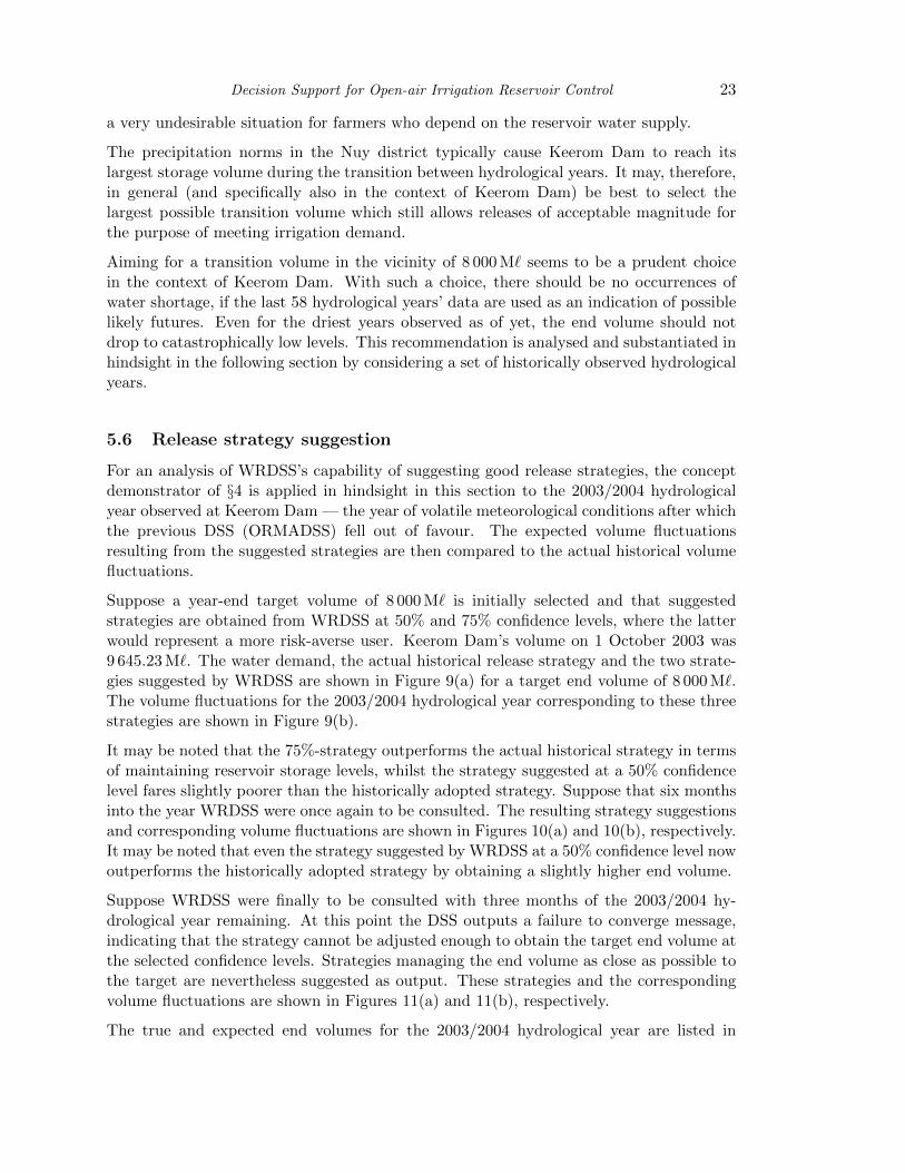
Suppose a year-end target volume of 8 000 M` is initially selected and that suggestedstrategies are obtained from WRDSS at 50% and 75% confidence levels, where the latterwould represent a more risk-averse user. Keerom Dam’s volume on 1 October 2003 was9 645.23 M`. The water demand, the actual historical release strategy and the two strate-gies suggested by WRDSS are shown in Figure 9(a) for a target end volume of 8 000 M`.The volume fluctuations for the 2003/2004 hydrological year corresponding to these threestrategies are shown in Figure 9(b).

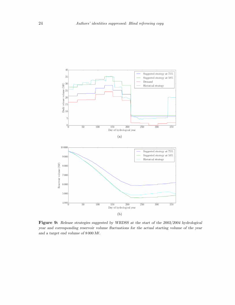
It may be noted that the 75%-strategy outperforms the actual historical strategy in termsof maintaining reservoir storage levels, whilst the strategy suggested at a 50% confidencelevel fares slightly poorer than the historically adopted strategy. Suppose that six monthsinto the year WRDSS were once again to be consulted. The resulting strategy suggestionsand corresponding volume fluctuations are shown in Figures 10(a) and 10(b), respectively.It may be noted that even the strategy suggested by WRDSS at a 50% confidence level nowoutperforms the historically adopted strategy by obtaining a slightly higher end volume.

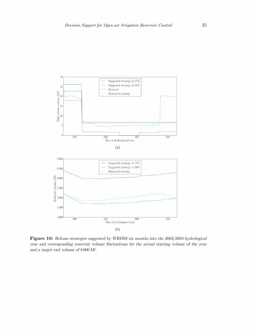
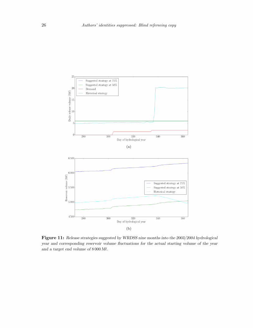
Suppose WRDSS were finally to be consulted with three months of the 2003/2004 hy-drological year remaining. At this point the DSS outputs a failure to converge message,indicating that the strategy cannot be adjusted enough to obtain the target end volume atthe selected confidence levels. Strategies managing the end volume as close as possible tothe target are nevertheless suggested as output. These strategies and the correspondingvolume fluctuations are shown in Figures 11(a) and 11(b), respectively.

The true and expected end volumes for the 2003/2004 hydrological year are listed in


(a)

(b)

Figure 9: Release strategies suggested by WRDSS at the start of the 2003/2004 hydrological

year and corresponding reservoir volume fluctuations for the actual starting volume of the year

and a target end volume of 8 000 M`.


(a)

(b)

Figure 10: Release strategies suggested by WRDSS six months into the 2003/2004 hydrological




(a)

(b)

Figure 11: Release strategies suggested by WRDSS nine months into the 2003/2004 hydrological




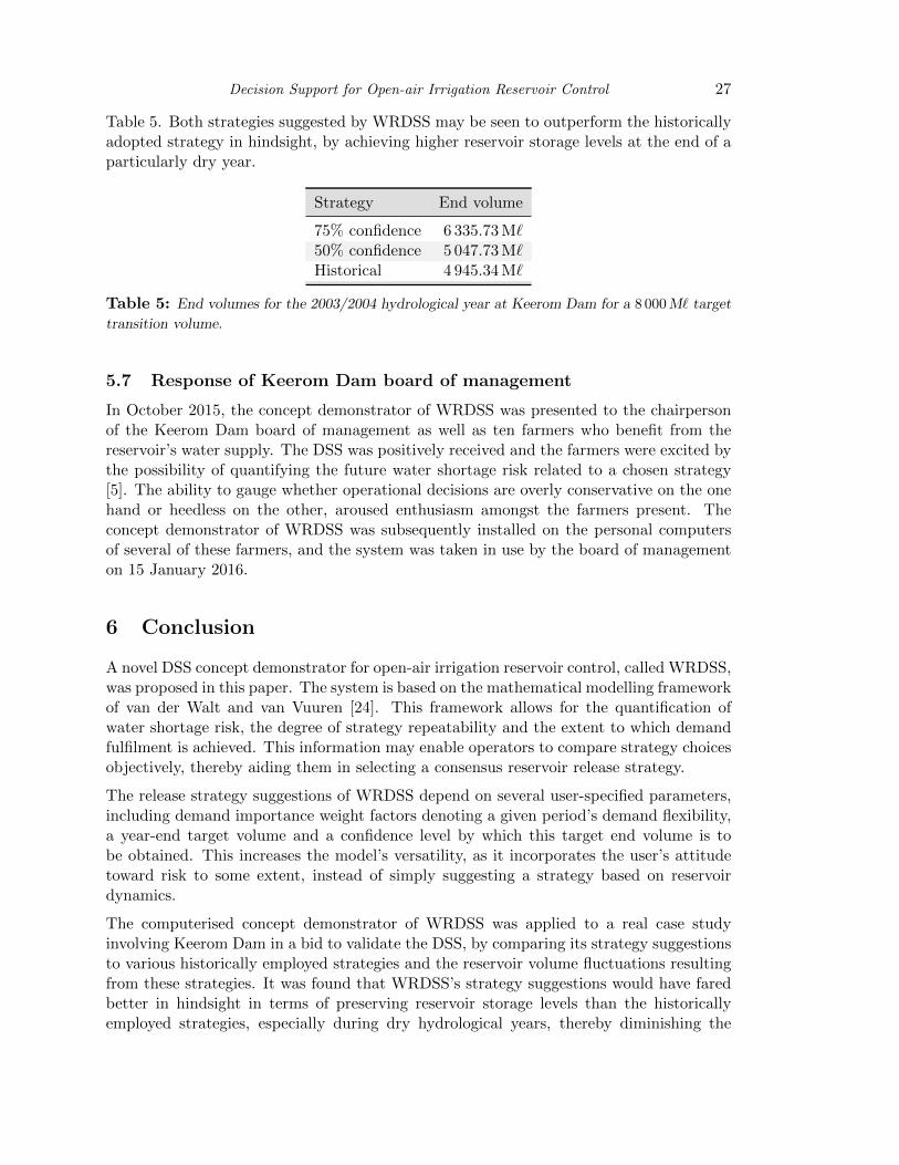
Table 5. Both strategies suggested by WRDSS may be seen to outperform the historicallyadopted strategy in hindsight, by achieving higher reservoir storage levels at the end of aparticularly dry year.

Strategy End volume

75% confidence 6 335.73 M`50% confidence 5 047.73 M`Historical 4 945.34 M`

Table 5: End volumes for the 2003/2004 hydrological year at Keerom Dam for a 8 000 M` target

transition volume.

5.7 Response of Keerom Dam board of management

In October 2015, the concept demonstrator of WRDSS was presented to the chairpersonof the Keerom Dam board of management as well as ten farmers who benefit from thereservoir’s water supply. The DSS was positively received and the farmers were excited bythe possibility of quantifying the future water shortage risk related to a chosen strategy[5]. The ability to gauge whether operational decisions are overly conservative on the onehand or heedless on the other, aroused enthusiasm amongst the farmers present. Theconcept demonstrator of WRDSS was subsequently installed on the personal computersof several of these farmers, and the system was taken in use by the board of managementon 15 January 2016.

6 Conclusion

A novel DSS concept demonstrator for open-air irrigation reservoir control, called WRDSS,was proposed in this paper. The system is based on the mathematical modelling frameworkof van der Walt and van Vuuren [24]. This framework allows for the quantification ofwater shortage risk, the degree of strategy repeatability and the extent to which demandfulfilment is achieved. This information may enable operators to compare strategy choicesobjectively, thereby aiding them in selecting a consensus reservoir release strategy.

The release strategy suggestions of WRDSS depend on several user-specified parameters,including demand importance weight factors denoting a given period’s demand flexibility,a year-end target volume and a confidence level by which this target end volume is tobe obtained. This increases the model’s versatility, as it incorporates the user’s attitudetoward risk to some extent, instead of simply suggesting a strategy based on reservoirdynamics.

The computerised concept demonstrator of WRDSS was applied to a real case studyinvolving Keerom Dam in a bid to validate the DSS, by comparing its strategy suggestionsto various historically employed strategies and the reservoir volume fluctuations resultingfrom these strategies. It was found that WRDSS’s strategy suggestions would have faredbetter in hindsight in terms of preserving reservoir storage levels than the historicallyemployed strategies, especially during dry hydrological years, thereby diminishing the


farmers’ exposure to water shortage risk. The concept demonstrator was received withpositive enthusiasm by the members of the Keerom Dam board of management who took itin use for strategy suggestion. The objective manner in which strategies can be compared,as facilitated by the quantitative performance metrics calculated by WRDSS, was notedas a significant benefit by members of the board.

In WRDSS, expected volumes are estimated using possible volume fluctuations basedon historically observed inflows. Previous models employed at Keerom Dam estimatedvolumes using inflow averages instead. The reservoir volume is, however, a non-linearfunction of inflows and release volumes, since evaporation losses are proportional to thereservoir’s exposed water surface area, which is a non-linear function of the reservoirstorage volume, and since the reservoir volume may only increase up to its maximumstorage capacity. More specifically, for a given fixed release strategy, the limits of possiblehydrological year-end volumes, based on historically observed inflow data, are concavefunctions of the total annual inflow, up to the reservoir storage capacity. According toJensen’s well-known inequality [4], the expected value of a concave function of a randomvariable is not greater than the concave function evaluated at the expected value of therandom variable. In the context of this paper, reservoir inflow is a random variableand the expected reservoir volume is a concave function of this variable. The model onwhich the WRDSS is based is therefore expected to produce more conservative, and morerealistic, volume estimations than previous models, because estimations are performed onthe function values, instead of on the variable values themselves. The standard approachof utilising historical cumulative inflow distributions for discrete simulation periods in aMonte Carlo simulation setting was analysed in the context of Keerom Dam and foundto be an insufficient representation of inflow behaviour. It was determined that historicalinflows, which represent existing knowledge on inflow behaviour, should instead be utiliseddirectly in the model.

7 Future work

Various ideas for future work, which may be pursued as extensions to the work documentedin this paper, are mentioned in this final section. A cost-benefit analysis may be performedin order to gain a concrete understanding of the financial implications of experiencingwater shortage. The influence of the shortage magnitude, duration and time of occurrencemay thus be investigated. Such information may perhaps be utilised in the selection ofdemand-importance weights to be used in WRDSS. An analysis of inflow variation mayalso be performed in respect of a number of large irrigation reservoirs so as to gain anunderstanding of a reservoir’s role either as buffer in terms of limiting outflows or as asource of security in hedging farmers against water shortage risk. In this paper, it wasobserved in the case of Keerom Dam that the volatility of annual inflow volumes is soextreme that mean inflow values are of little use. Since the effects of small annual inflowsdiffer vastly from the effects of large annual inflows, considering only standard deviationis not adequate.

As WRDSS was developed with the intention of being a generic DSS for the selection ofwater release strategies at open-air irrigation reservoirs, it may be applied to case studies


other than that of Keerom Dam in order to explore its flexibility in terms of suggestinggood water release strategies.

A study may further be performed to determine beneficial release strategies at large waterreservoirs, in the presence of a network of smaller secondary reservoirs located downstream.In the case of Keerom Dam, for example, all of the farmers who benefit from water fromthe reservoir also have smaller dams on their farms in which they can store water releasedfrom Keerom Dam. These secondary reservoirs may differ in size and may each havea unique demand profile. Methods for the aggregation of these demand profiles into ademand profile for the larger, upstream reservoir may also be investigated.

The functionality of WRDSS may finally be extended to consider strategy formulation overscheduling horizons exceeding one year. The effects of a given strategy on storage levelswhen considering N ∈ {1, 2, 3, . . .} consecutive hydrological years’ inflows may be analysedto determine an explicit, non-conditional N -year water shortage risk corresponding to agiven transition volume.

References

[1] Bontemps C & Couture S, 2002, Irrigation water demand for the decision maker, Environmentand Development Economics, 7(4), pp. 643–657.

[2] Box GE & Jenkins GM, 1976, Time series analysis: Forecasting and control, 2nd Edition, Holden-Day, San Francisco (CA).

[3] Burden RL & Faires JD, 1989, Numerical analysis, PWS Kent Publishing Co., Boston (MA).

[4] Chandler D, 1987, Introduction to modern statistical mechanics, Oxford University Press, Oxford.

[5] Conradie A, 2015, Chairperson of the Keerom Dam Board of Management, Personal Communica-tion.

[6] Department of Water Affairs and Forestry, 2015, Hydrology database, [Online],[Cited August 17th, 2015], Available from http://www:dwa:gov:za/Hydrology/HyStations:

aspx?River=Nuy&StationType=rbReservoirs

[7] Human O & Hagen DJ, 2014, Raising of Keerom Dam, (Unpublished) Technical Report9523/107752,Aurecon South Africa (Pty) Ltd., Cape Town.

[8] Jain S, Das A & Srivastava D, 1999, Application of ANNs for reservoir inflow prediction andoperation, Journal of Water Resources Planning and Management, 125(5), pp. 263–271.

[9] Jianping H, Yuhong Y, Shaowu W & Jifen C, 1993, An analogue-dynamical long-range nu-merical weather prediction system incorporating historical evolution, Quarterly Journal of the RoyalMeteorological Society, 119(511), pp. 547–565.

[10] Keen PG, 1987, Decision support systems: The next decade, Decision Support Systems, 3(3), pp. 253–265.

[11] Kelton WD & Law AM, 2000, Simulation modeling and analysis, McGraw-Hill, Boston (MA).

[12] Rizzo ML, 2008, Statistical computing with R, Chapman & Hall/CRC, London.

[13] SciPy.org, 2014, [Online], [Cited August 24th, 2015], Available from http://docs.scipy.org/

doc/numpy/reference/generated/numpy.polynomial.polynomial.polyfit.html

[14] Shim JP, Warkentin M, Courtney JF, Power DJ, Sharda R & Carlsson C, 2002, Past,present, and future of decision support technology, Decision Support Systems, 33(2), pp. 111–126.

[15] Smith M, Allen R & Pereira L, 1998, Revised FAO methodology for crop-water requirements,(Unpublished) Technical Report ISSN 1011-4289, Joint FAO/IAEA Division of Nuclear Techniquesin Food and Agriculture, Vienna.


[16] Strauss JC, 2014, A decision support system for the release strategy of an open-air irrigation reser-voir, Final-year Project, Department of Industrial Engineering, Stellenbosch University, Stellenbosch.

[17] Sun YH, Yang S, Yeh WW & Louie PW, 1996, Modeling reservoir evaporation losses by generalizednetworks, Journal of Water Resources Planning and Management, 122(3), pp. 222–226.

[18] Sudheer K, Gosain A, Mohana Rangan D & Saheb S, 2002, Modelling evaporation using anartificial neural network algorithm, Hydrological Processes, 16(16), pp. 3189–3202.

[19] Swennenhuis J, 2006, CROPWAT version 8.0, [Online], [Cited April 30th, 2015], Available fromhttp://www:fao:org/nr/water/infores databases cropwat.html.

[20] Taleb NN, 2012, Antifragile: Things that gain from disorder, Random House Incorporated, NewYork (NY).

[21] Tibane E & Vermeulen A, 2014, South Africa Yearbook 2013/14, [Online], [Cited March 9th, 2015],Available from http://www:gcis:gov:za/content/resourcecentre/sa-info/yearbook2013-14.

[22] Rumbaugh J, Jacobson I & Booch G, 2004, Unified modeling language reference manual, 2nd

Edition, Pearson Higher Education, Boston (MA).

[23] van Heerden P, Crosby C, Grove B, Benade N, Theron E, Schulze R & Tewolde M, 2009,Integrating and updating of SAPWAT and PLANWAT to create a powerful and userfriendly irrigationplanning tool, (Unpublished) Technical Report TT 391/08, Water Research Commission, Gezina.

[24] van der Walt JC & van Vuuren JH, 2015, Decision support for the selection of water releasestrategies at open-air irrigation reservoirs, Proceedings of the 44th Annual Conference of the Opera-tions Research Society of South Africa, Hartbeespoort, pp. 33–43.

[25] van Vuuren JH & Grundlingh WR, 2001, An active decision support system for optimality in openair reservoir release strategies, International Transactions in Operational Research, 8(4), pp. 439–464,

[26] Willis DB & Whittlesey NK, 1998, The effect of stochastic irrigation demands and surface watersupplies on on-farm water management, Journal of Agricultural and Resource Economics, 23, pp. 206–224.

[27] Wilks DS & Wilby RL, 1999, The weather generation game: A review of stochastic weather models,Progress in Physical Geography, 23(3), pp. 329–357.

[28] Winter TC, 1981, Uncertainties in estimating the water balance of lakes, JAWRA Journal of theAmerican Water Resources Association, 17(1), pp. 82–115.

decision support for open-air irrigation reservoir control of 450 mm ... open-air reservoirs are...

Documents