irrigation water requirement estimation decision...
TRANSCRIPT

The University of Hawai’i at Mānoa Department of Natural Resources and Environmental Management
College of Tropical Agriculture and Human Resources, University of Hawaii-Manoa
Irrigation Water Requirement Estimation Decision Support System
(IWREDSS) to Estimate Crop Irrigation Requirements for Consumptive
Use Permitting In Hawaii
Final Report
August 2013
Prepared for:
STATE OF HAWAII DEPARTMENT OF LAND AND NATURAL RESOURCES
COMMISSION OF WATER RESOURCES MANAGEMENT P.O. BOX 621
Honolulu, HI 96809
Submitted by:
Ali Fares, PhD
Professor of Watershed Hydrology and Tropical Soils,
Department of Natural Resources and Environmental Management,
College of Tropical Agriculture and Human Resources,
University of Hawai`i at Mānoa,
1910 East-West Road, Honolulu, HI 96822

i
EXECUTIVE SUMMARY
This report gives a detailed over view version 2.0 of the Irrigation Water Requirement
Estimation Decision Support System (IWREDSS, 2.0) – an ArcGIS-based numerical simulation
model was developed to help estimate crop irrigation requirements for consumptive use
permitting in Hawaii. The model estimates irrigation requirements (IRR) for perennial and
annual crops grown on Hawaiian soils. The model estimates IRR and other water budget
components including net irrigation water requirements (NIR), gross irrigation water
requirements (GIR), water duty in inches of 1000 gallons per acre (GAL_A), gross rain
(G_RAIN), net rain (N_RAIN), effective rain (ER), runoff (RO), canopy interception (INT),
potential evapotranspiration (ETO), reference evapotranspiration (ETC), and drainage (DR). The
model uses various irrigation application systems (i.e., trickle-drip, trickle-spray, multi sprinkler,
nursery/container sprinkler, large gun sprinkler, seepage/sub irrigation, crown flood, and flood
(Taro)), growing seasons, and irrigation practices (e.g. the usual practice of irrigating to field
capacity, applying a fixed depth per irrigation event, and deficit irrigation).
IWREDSS uses different databases for weather, crop water uptake parameters, irrigation
systems, and soil physical properties. These databases and other information used in IWREDSS
are summarized in this report and include 1) potential evapotranspiration, 2) rainfall 3) soil
physical properties, e.g., water holding capacities, and 5) crop water up take parameters (length
of growing season, crop coefficient, and rooting depth).
IWREDSS 1.0 runs as an extension of the ESRI ArcGIS 9.2 software and IWREDSS 2.0
runs as an Adds-In of the ESRI ArcGIS 10.x. This report includes a step by step guide on how to
use IWREDSS to simulate IRRs for a specific area based on its Tax Map Key ( called in this
document TaxID), or included in a digitized may as a GIS layer. IWREDSS results are presented
in a text (ASCII) file and graphically as a GIS layer/map.
IWRDESS was calibrated and validated with irrigation data estimates from Hawaii
USDA-NRCS Handbook 38 (USDA-NRCS, 1996). These data include irrigation requirements
maps for some crops on the major Hawaiian Islands. A sensitivity analysis was also carried out to
test the effect of the timing of growing seasons on the IRRs for seed corn (a four month growing
ii
season) with twelve different starting dates throughout the year (January through December).
IRR estimations were also calculated for different bioenergy crops under windward and leeward
conditions on the islands of Maui, Kauai, Oahu, and Hawaii. Irrigation requirements calculated
with IWREDSS for different crops grown under specific to Hawaiian Islands are in close
agreement with those estimated by USDA-NRCS Handbook 38. The relative small differences
between the two datasets could be due to several factors including spatial and temporal
variability of rainfall, evapotranspiration, and soil physical properties, and interpolation methods
used to estimate rainfall and evapotranspiration.
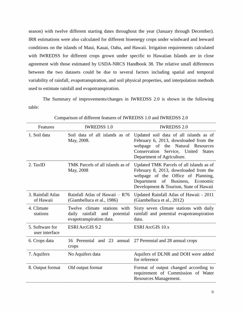
The Summary of improvements/changes in IWREDSS 2.0 is shown in the following
table:
Comparison of different features of IWREDSS 1.0 and IWREDSS 2.0
Features IWREDSS 1.0 IWREDSS 2.0
1. Soil data Soil data of all islands as of
May, 2008.
Updated soil data of all islands as of
February 6, 2013, downloaded from the
webpage of the Natural Resources
Conservation Service, United States
Department of Agriculture.
2. TaxID TMK Parcels of all islands as of
May, 2008
Updated TMK Parcels of all islands as of
February 8, 2013, downloaded from the
webpage of the Office of Planning,
Department of Business, Economic
Development & Tourism, State of Hawaii
3. Rainfall Atlas
of Hawaii
Rainfall Atlas of Hawaii – R76
(Giambelluca et al., 1986)
Updated Rainfall Atlas of Hawaii - 2011
(Giambelluca et al., 2012)
4. Climate
stations
Twelve climate stations with
daily rainfall and potential
evapotranspiration data.
Sixty seven climate stations with daily
rainfall and potential evapotranspiration
data.
5. Software for
user interface
ESRI ArcGIS 9.2 ESRI ArcGIS 10.x
6. Crops data 16 Perennial and 23 annual
crops
27 Perennial and 28 annual crops
7. Aquifers No Aquifers data Aquifers of DLNR and DOH were added
for reference
8. Output format Old output format Format of output changed according to
requirement of Commission of Water
Resources Management.

iii
TABLE OF CONTENTS
Contents Page
EXECUTIVE SUMMARY i
TABLE OF CONTENTS iii
GLOSSARY 1
1. INTRODUCTION 1
2. REVIEW OF LITERATURE 3
3. DATABASES 4
3.1 Crop factors 5
3.2 Climate stations 5
3.2.1 Rainfall 11
3.2.2 Potential evapotranspiration (ETo) 11
3.3 Soil data 12
3.4 GIS data 13
3.4.1 Soil data 13
3.4.2 TaxID 13
3.4.3 Soil statistic dataset 13
3.4.4 Rainfall grid 13
3.4.5 Potential evaporation grid 14
3.4.6 Climate stations 14
3.4.7 Aquifers 14
4. CALIBRATION AND VALIDATION 14
5. PLOTTING THE MODEL RESULTS 16
6. SENSIVITY ANALYSIS 16
6.1 Effect of crop leaf area index on irrigation allocations 18
7. SIMULATION USING ENERGY CROPS 19
8. SUMMARY AND CONCLUSION 22
9. REFERENCES 23
10. APPENDICES 26
11. USER’ MANUAL 26
12. TECHNICAL GUIDE 46
Tables
Table 1 Annual crop effective root depth, KC values and stage lengths as a fraction of growing
Period 6
Table 2 Perennial crop effective root depth and KC values by month of the year 7
Table 3 Detailed information of the climate stations used in the database 8
Table 4 Calibration and validation 15
Table 5 Sweet corn: Acreage, yield, production, price, and value, in Hawaii, 1999-2008 17
Table 6 Energy crops and growing seasons selected for simulating irrigation requirements 20
Table 7 Net irrigation requirements (in) for energy crops grown on windward and
leeward sides of the islands in dry and wet seasons 20
Table 8 Percent difference in the NIR calculated for energy crops during dry and wet seasons 21

iv
Figures
Figure 1 Comparison of annual average rainfall (database, IWREDSS vs. grid value
derived from Rainfall Atlas of Hawaii, 2011). 11
Figure 2 Scatter plot of annual average ETo after adjustment of 56 stations based on
PE grid and 11 stations based on annual average PE of the station 12
Figure 3 Validation of IWREDSS with USDA-NRCS results 16
Figure 4 Changes in NIR based on changes in growing periods for seed corn grown
on windward (Waimanalo) and leeward (Kunia) sides of Oahu. 18
Figure 5 Net irrigation requirements (NIR) and effective rain (ER) versus
leaf area index (LAI) 19
Figure 6 Percent change in Net irrigation requirements (NIR, open symbol)
and effective rain (ER, closed symbol) with leaf area index (LAI). 19
Figure 7 Irrigation requirements for (a) corn and (b) sugarcane 21
Appendices
Appendix 1 User Manual 26
Appendix 2 Technical Guide 46
Appendix 3 Calculation of daily ETo using temperature data 59
Appendix 4a Climate data stations for the island of Kauai. Station information is in Table 3.
Isohyets indicate gradients in rainfall (dark) and elevation (light) 60
Appendix 4b Climate data stations for the island of Oahu and Molokai. Station information is in
Table 3. Isohyets indicate gradients in rainfall (dark) and elevation (light). 61
Appendix 4c Climate data stations for the island of Maui and Lanai. Station information is in
Table 3. Isohyets indicate gradients in rainfall (dark) and elevation (light). 62
Appendix 4d Climate data stations for the Island of Hawaii. Station information is in Table 3.
Isohyets indicate gradients in rainfall (dark) and elevation (light) 63
Appendix 5a Seasonal water budget components 64
Appendix 5b Statistics for seasonal gross and net irrigation requirements 66

1
GLOSSARY:
ALISH: Agricultural Lands of Importance to the State of Hawaii.
AWD (Allowable Water Depletion): Fraction of the available soil water storage capacity that
can be allowed to deplete without significant reduction in crop yield.
DR (Drainage): Portion of incoming water that drains below plant root zone.
ER (Effective Rain): Portion of water that is stored in the root zone and used by the plants.
ETC (Reference Evapotranspiration): Portion of water that vaporizes back to the atmosphere
via plants. The ETC is the amount of ETO occurring from a specific crop.
ETO (Potential Evapotranspiration): Evapotranspiration to the given atmospheric conditions.
G_RAIN (Gross Rain): The rain that falls from the clouds and reaches the crown of plants.
GAL_A: Water duty in inches of 1000 gallons per acre.
GIR (Gross Irrigation Requirements): NIR divided by the application efficiency of irrigation
application system.
GIS: Geographic information system.
INT (Canopy Interception): Portion of G_RAIN intercepted by the plant canopy or crown.
IWREDSS: Irrigation Water Requirement Estimation Decision Support System.
IRR: Irrigation requirements
KC: Crop coefficient.
LAI (Leaf Area Index): Ratio of total upper leaf surface of vegetation divided by the surface
area of the land on which the vegetation grows.
LSB: Island-wide simulation using Land Study Bureau Classification.
N_RAIN (Net Rain): The volume of rainfall that reaches the soil and comprises throughfall
and stemflow.
NIR (Net Irrigation Requirements): Irrigation requirements estimated by model without
accounting for irrigation losses.
PE: Open pan evaporation
RO (Runoff): Portion of incoming water that runs off to the low level areas.
SCS CN (Soil Conservation Services Curve Number): It is related to the imperviousness of a
surface; for impervious and water surfaces CN=100, for natural surfaces CN < 100.
1. INTRODUCTION
This report gives an overview of the update of the Irrigation Water Requirement Estimation
Decision Support System (IWREDSS, V 2.0) for the determination of reasonable water use
quantities for selected crops across the major Hawaiian islands. IWREDSS estimates net and
gross irrigation requirements (NIR and GIR, respectively) for different crops grown on specific
soils, irrigated with a given irrigation system, grown during a specific time of the year, and under
defined climate conditions. The irrigation requirement (IRR) of a crop is the amount of water, in
addition to precipitation, that a crop needs to meet its evapotranspiration (ET) demand. The

2
irrigation requirements do not account for leaching, freeze protection, or crop cooling
requirements, even though water for these purposes may be applied through an irrigation system.
IWREDSS is an ArcGIS based software, and its interface enables users to choose input
data and display results. The user selects the area of interest based on its TaxID, or included in a
digitized may as a GIS layer. Then the user chooses various options from drop down menus of
the interface to select the crop to be grown/irrigated, crop leaf area index (LAI), the growing
season, irrigation system to be used, and the curve number for the soil type / land use. The
program accesses the weather and soil physical database library and interpolates rainfall and ET
data based on location of the nearest weather station with respect to the area of interest. These
interpolated data are then used for the IRR calculation. Up on the successful execution of the
program, the users are given the option to retrieve the results in the form of a text (ASCII) file or
displayed as a GIS map.
Recent developments in GIS systems present the opportunity to apply physically based
soil water balance and simulation models at a regional scale (Satti et al, 2004). Satti and Jacobs
(2004) developed GWRAPPS (GIS-based Water Resources and Agricultural Permitting and
Planning System) model by coupling AFSIRS model (Smajstrla and Zazueta, 1988) with GIS.
CropSyst (Stockle et al., 1994), AEGIS/WIN (Engel et al., 1997), and GWRAPPS are models
that simulate the soil water budget components (WBC) by coupling crop parameters with soil
and long-term climate databases. The estimation of IRR using IWREDSS requires databases of
soils, crops, rainfall, ET, and other information. Geographical Information System has been
employed to integrate these databases. These databases can be used repeatedly and can also be
updated when new information becomes available.
This report covers the following deliverables.
Databases of the IWREDSS elements and parameters
GIS island maps showing NOAA climate stations used to develop the rainfall and ET
databases.
A DVD containing tested version of IWREDSS
Results of IWREDSS calibration and validation
Results of IWREDSS sensitivity analysis
Testing of IWREDSS using energy crops
IWREDSS user manual
IWREDSS technical guide

3
The user’s manual and the technical guide for IWREDSS are two separate documents;
they are in appendices 1 and 2, respectively.
2. REVIEW OF LITERATURE
Numerical models for water management track the water budget of the soil-plant-atmosphere
system; however, such models require large amounts of computation, time and data storage.
Most importantly, data required for such detailed models are not available for all of the
production systems of interest. The use of a real-time simulation model to increase accuracy is
not justified. Thus, IWREDSS uses a daily soil water budget to calculate crop IRRs.
Technical Release 21, and empirical method developed by the Soil Conservation Service
(SCS, 1970), estimates monthly IRR based on monthly average rainfall and ET, and on soil
water-holding capacity. However, IWREDSS model integrates the effects of day-to-day
distributions of rainfall, ET, and soil water-holding capacity to calculate IRRs.
Since the 1980’s, the regional water management districts of Florida have been using this
daily water budget approach. Melaika and Bottcher (1988) applied this approach to model
nutrient movement from a South Florida watershed in the Everglades Agricultural Area.
Villalobos and Fereres (1989) developed a water budget model based on long-term average
potential ET and actual rainfall data. In their model, potential ET was assumed to be constant
each year because long-term data were not available. Samani et al. (1987) used a water budget
approach to develop a crop yield model. They simulated weather data because long-term climate
data were not available.
Agricultural engineers recommend the water budget approach for the development of a
basic irrigation scheduling model for Florida conditions (Smajstrla et al., 1988a). This approach
was also used to develop a Florida citrus micro irrigation scheduling model (Smajstrla et al.,
1987). Smajstrla and Zazueta (1987) demonstrated data requirements and sensitivity of the water
budget approach to determine irrigation requirements of Florida nursery and agronomic crops.
Some water budget models were developed for specific crops, e.g., Brown et al. (1978),
Odhiambo and Murty (1996), and Mishra (1999) worked on rice water balance. Pereira (1989)
developed the rice water balance model IRRICEP and tested its performance against field data.

4
Paulo et al. (1995) validated the IRRICEP model using historical data on water use for selected
sectors of Sorraia irrigation system in Brazil. Shah and Edling (2000) used the water balance
approach to calculate daily ET from a flooded rice field using measured values of water level,
rain, irrigation, seepage, and tail water runoff. Khepar et al. (2000) developed a water balance
model applicable to intermittent irrigation practice in rice fields by incorporating saturated and
unsaturated water flow concepts to predict deep percolation loss during wet and dry periods.
Many of water budget models lack user-friendly interfaces except few of them; these
models offer limited flexibility in selecting a suitable method for estimating potential
evapotranspiration. George et al. (2000) developed a user-friendly model (ISM) for field crops.
Efforts have been exerted to couple user-friendly interfaces with Geographical Information
Systems for efficient and quick data handling. Knox et al. (1996, 1997) developed a procedure
for mapping the spatial distribution of crop irrigation water requirements based on crop
parameters, climate and soil data in UK. Weatherhead and Knox (2000) developed a
methodology for predicting future growth in irrigation water demand in countries with
supplemental irrigation such as England and Wales using GIS. The GIS based water- and salt-
balance studies at irrigation district level have also been attempted (Young and Wallender,
2002). George et al. (2004) used GIS to include spatial and extensive input information for their
irrigation scheduling model.
These models compute the water budget for a specific field, one crop, and a complete
growing season (monthly basis). In addition to simulation for an enhanced period of time,
estimating IRRs on daily and weekly basis is needed. IWREDSS is based on the same approach
used in the agricultural field scale irrigation requirements simulation (AFSIRS) model (Smajstrla
and Zazueta, 1988). IWREDSS calculates IRRs on weekly, bi-weekly, monthly and year bases;
more output options are also available with the non-GIS version of the model IManSys (Fares
and Fares, 2012). IWREDSS needs spatially distributed historical input data. Databases were
developed encompassing the information required by IWREDSS for Hawaii conditions.
3. DATABASES
IWREDSS databases include historical daily potential evapotranspiration and rainfall for
different locations across the major five Hawaiian Islands. The range of these two databases is

5
variable across the different locations. In addition, the model uses the crop database that includes
all crop coefficients and root development parameters. Databases of crop factors, climate
stations, soil and GIS data were updated in version 2.0 of the software. Brief description of each
database is discussed here.
3.1 Crop factors
Crop parameters including effective rooting depths, crop coefficients (Kc), duration of cropping
season, allowable water depletion for 29 major annual (Table 1) and 28 perennial (Table 2) crops
grown on Hawaii are provided along with common irrigation systems and their corresponding
irrigation efficiencies. Nine perennial crops and four annual crops were added to the dataset in
IWREDSS 2.0.
3.2 Climate stations
Databases of daily rainfall, minimum and maximum temperature of 67 locations across the
Hawaiian Islands were collected from the National Oceanic and Atmospheric Administration,
National Climatic Data Center, NOAA, NCDC, (http://www.ncdc.noaa.gov/cdo-
web/#t=firstTabLink). The major criterion used to select climate stations is the length of the
period of their recorded data. We selected the stations with at least 19 years long data record.
Twenty nine stations have more than 50 year data; whereas, 38 stations have data record between
19 and 50 years.

6
Table 1. Annual crop effective root depth, Kc values and stage lengths as a fraction of growing period
Crop Root depth (in)
Kcinitial Kcmid Kclate Duration (fraction of crop cycle) Allowable water depletion (fraction of total) Irrigation
type
Irrigation
efficiency (%) Initial Final Stage 1 Stage 2 Stage 3 Stage 4 Stage 1 Stage 2 Stage 3 Stage 4
Alfalfa, initial 8 24 0.4 0.95 0.9 0.14 0.38 0.31 0.17 0.5 0.5 0.5 0.5 Sprinkler 70
Alfalfa, ratoon 24 24 0.4 0.95 0.9 0.14 0.38 0.31 0.17 0.5 0.5 0.5 0.5 Sprinkler 70
Bana Grass (Sudan), 1st cut 18 36 0.5 0.9 0.85 0.33 0.33 0.2 0.14 0.5 0.5 0.5 0.5 Sprinkler 70
Bana Grass (Sudan), 2nd cut 36 36 0.5 1.15 1.1 0.08 0.4 0.32 0.19 0.5 0.5 0.5 0.5 Sprinkler 70
Banana, initial 24 48 0.5 1.1 1 0.31 0.23 0.31 0.15 0.35 0.35 0.35 0.35 Micro-spray 80
Banana, ratoon 48 48 1 1.05 1.05 0.33 0.16 0.49 0.01 0.35 0.35 0.35 0.35 Micro-spray 80
Cabbage 8 12 0.7 1.05 0.95 0.24 0.36 0.3 0.09 0.45 0.45 0.45 0.45 Drip 85
Cantaloupe 8 12 0.5 0.85 0.6 0.08 0.5 0.21 0.21 0.35 0.35 0.35 0.35 Drip 85
Dry Onion 8 12 0.7 1.05 0.75 0.1 0.17 0.5 0.23 0.25 0.25 0.25 0.9 Drip 85
Eggplant 8 12 0.7 1.05 0.9 0.21 0.32 0.29 0.18 0.4 0.4 0.4 0.4 Drip 85
Ginger (AWD potatoes) 8 12 0.7 1.05 0.75 0.1 0.17 0.5 0.23 0.25 0.25 0.25 0.25 Drip 85
Lettuce 8 12 0.7 1 0.95 0.2.7 0.4 0.2 0.13 0.3 0.3 0.3 0.3 Sprinkler 70
Other melon 8 12 0.5 1.05 0.75 0.21 0.29 0.33 0.17 0.35 0.35 0.35 0.35 Drip 85
Peanuts 12 18 0.4 1 0.55 0.25 0.32 0.25 0.18 0.5 0.4 0.5 0.5 Drip 85
Peppers 8 12 0.4 0.95 0.8 0.24 0.28 0.32 0.16 0.35 0.35 0.35 0.35 Drip 85
Pineapple, year 1 12 12 0.5 0.3 0.3 0.16 0.33 0.26 0.25 0.6 0.6 0.6 0.6 Drip 85
Pineapple, year 2 24 24 0.3 0.3 0.3 0.38 0.32 0.27 0.03 0.6 0.6 0.6 0.6 Drip 85
Pumpkin 8 12 0.5 1 0.8 0.2 0.3 0.3 0.2 0.35 0.35 0.35 0.5 Drip 85
Seed Corn 12 18 0.4 1.2 0.5 0.16 0.28 0.32 0.24 0.6 0.6 0.6 0.8 Drip 85
Soybean 12 18 0.4 1.05 0.45 0.14 0.25 0.43 0.18 0.5 0.5 0.5 0.67 Drip 85
Sugarcane, ratoon 36 36 0.4 1.25 0.75 0.1 0.15 0.46 0.29 0.65 0.65 0.65 0.65 Drip 85
Sugarcane, New- year 1 18 36 0.4 1.25 1.25 0.21 0.29 0.25 0.25 0.65 0.65 0.65 0.65 Drip 85
Sugarcane, New- year 2 36 36 1.25 1.25 0.75 0.14 0.14 0.14 0.59 0.65 0.65 0.65 0.65 Drip 85
Sunflowers 12 18 0.4 1.05 0.4 0.16 0.28 0.36 0.2 0.45 0.45 0.45 0.67 Drip 85
Sweet potato 8 12 0.5 1.15 0.65 0.12 0.24 0.4 0.24 0.65 0.65 0.65 0.65 Drip 85
Taro (Dry) 12 18 1.05 1.15 1.1 0.2 0.13 0.4 0.27 0.3 0.3 0.3 0.3 Drip 85
Taro (Wet) 12 18 1.25 1.25 1.25 0.2 0.13 0.4 0.27 0 0 0 0 Flood 50
Tomato 8 12 0.6 1.15 0.8 0.2 0.27 0.34 0.19 0.4 0.4 0.4 0.65 Drip 85
Watermelon 8 12 0.4 1 0.75 0.15 0.26 0.26 0.32 0.26 0.32 0.26 0.32 Drip 85

7
Table 2. Perennial crop effective root depth and KC values by month of the year
Crop Rootzone depth, in
Jan Feb Mar Apr May Jun Jul Aug Sep Oct Nov Dec Irrigation type
Irrigation
efficiency
(%) Irrigated Total
Avocado 30 60 0.9 0.9 0.9 0.9 0.95 1 1 1 1 1 1 1 Drip 85
Bermuda grass 24 48 1 1 1 1 1 1 1 1 1 1 1 1 Sprinkler 0.75
Breadfruit 30 60 0.9 0.9 0.9 0.9 0.95 1 1 1 1 1 1 1 Drip 85
Citrus 30 40 0.56 0.62 0.71 0.78 0.82 0.86 0.88 0.87 0.85 0.81 0.75 0.67 Drip 85
Coconut, Palms 30 60 1 1 1 1 1 1 1 1 1 1 1 1 Drip 85
Coffee 24 48 0.85 0.85 0.85 0.9 0.95 0.95 0.95 0.95 0.95 0.95 0.9 0.9 Micro spray (MS) 0.8
Dendrobium, pot 8 8 1 1 1 1 1 1 1 1 1 1 1 1 MS; nursery sprinkler 0.80, 0.20
Dillisgrass 24 48 1 1 1 1 1 1 1 1 1 1 1 1 Sprinkler 0.75
Domestic Garden 1 1 1 1 1 1 1 1 1 1 1 1 1 1 Sprinkler 0.75
Draceana, pot 8 8 1 1 1 1 1 1 1 1 1 1 1 1 MS; nursery sprinkler 0.80, 0.20
Eucalyptus closed canopy 72 72 1 1 1 1 1 1 1 1 1 1 1 1 Micro spray 0.8
Eucalyptus young 48 72 0.6 0.6 0.6 0.6 0.6 0.6 0.6 0.6 0.6 0.6 0.6 0.6 Micro spray 0.8
Garden Herbs 12 24 1 1 1 1 1 1 1 1 1 1 1 1 Sprinkler 0.75
Guava 30 60 8 0.9 1 1 9 0.8 0.8 0.9 1 1 9 8.5 Micro spray 0.8
Heliconia 24 48 1 1 1 1 1 1 1 1 1 1 1 1 Micro spray 0.8
Kikuyu grass 24 48 1 1 1 1 1 1 1 1 1 1 1 1 Sprinkler 0.75
Koa 72 72 1 1 1 1 1 1 1 1 1 1 1 1 Micro spray 0.8
Leuceana (Old) 72 72 1 1 1 1 1 1 1 1 1 1 1 1 Micro spray 0.8
Leuceana (Young 48 72 0.6 0.6 0.6 0.6 0.6 0.6 0.6 0.6 0.6 0.6 0.6 0.6 Micro spray 0.8
Lychee 30 60 0.95 1 1 1 0.95 0.9 0.9 0.85 0.8 0.8 0.9 0.9 Micro spray 0.8
Macadamia nut 30 60 0.85 0.85 0.85 0.9 0.95 0.95 0.95 0.95 0.95 0.95 0.9 0.9 Micro spray 0.8
Mango 30 60 0.9 0.9 0.9 0.9 0.95 1 1 1 1 1 1 1 Drip 85
Papaya 25 37 0.42 0.42 0.42 0.42 0.42 0.42 0.42 0.42 0.42 0.42 0.42 0.42 Drip 85
St. Augustine 24 48 1 1 1 1 1 1 1 1 1 1 1 1 Sprinkler 0.75
Ti 24 48 1 1 1 1 1 1 1 1 1 1 1 1 Micro spray 0.8
Turf, Golf 9 24 1 1 1 1 1 1 1 1 1 1 1 1 Sprinkler 0.75
Turf, Landscape 12 24 1 1 1 1 1 1 1 1 1 1 1 1 Sprinkler 0.75
Zoysia grass 24 48 1 1 1 1 1 1 1 1 1 1 1 1 Sprinkler 0.75

8
Table 3. Detailed information of the climate stations used in the database.
S.
No. Climate Station
COOP
ID Island
Latitude
(oN)
Longitude
(oW)
Elevation
(m) From To
Annual
mean
rain (in)
Annual
mean
ETo (in)
Remarks
1 EWA PLANTATION 741 510507 Oahu 21.37472 157.99167 6.1 1950 2005 25.147 70.162 Data gap from 1997 to
2001.
2 HAINA 214 510840 Hawaii 20.10000 155.46667 140.5 1950 1993 75.109 68.234
3 HALEAKALA EXP FARM 510995 Maui 20.85000 156.30000 640.1 1950 1991 84.655 51.044
4 HALEAKALA RS 338 511004 Maui 20.76030 156.24700 2122.0 1950 2011 52.137 48.528
5 HANA AP 355 511125 Maui 20.79470 156.01540 22.9 1951 2011 80.292 52.644
6 HAWAII VOL NP 511303 Hawaii 19.42970 155.25620 1210.4 1950 2011 106.429 45.387
7 HILO INTL AP 511492 Hawaii 19.71910 155.05300 11.6 1950 2011 127.086 50.240
8 HONOLULU OBSERV. 702.2 511918 Oahu 21.31520 157.99920 0.9 1963 2011 19.671 68.159
9 HONOLULU INTL AP 511919 Oahu 21.32389 157.92944 2.1 1950 2011 20.363 68.442
10 HONOLULU SUBSTN 407 511924 Oahu 21.31667 157.86667 4.0 1950 1976 26.601 71.849
11 HONOMU MAUKA 138 511960 Hawaii 19.85000 155.15000 335.3 1950 1977 216.367 37.415
12 KAHUKU 912 512570 Oahu 21.69500 157.98111 4.0 1950 1972 50.530 65.616
13 KAHULUI AP 512572 Maui 20.89972 156.42861 15.5 1954 2011 18.293 75.474
14 KAILUA 446 512679 Maui 20.89050 156.21270 213.4 1950 2011 137.747 53.234
15 KAINALIU 73.2 512751 Hawaii 19.53360 155.92580 457.2 1950 2011 64.526 34.890
16 KAMUELA 192.2 513077 Hawaii 20.01667 155.66667 814.1 1951 1979 33.437 36.923
17 KANALOHULUHULU 1075 513099 Kauai 22.12972 159.65861 1097.3 1955 2011 66.733 33.841
18 KANEOHE MAUKA 781 513113 Oahu 21.41667 157.81667 57.9 1950 1997 77.365 35.581
19 KAPALUA W MAUI 513317 Maui 20.96250 156.67530 73.2 1987 2011 28.955 72.312
20 KAPOHO BEACH 93.11 513368 Hawaii 19.50140 154.82220 6.1 1977 2011 82.909 62.144
21 KEAAU 92 513872 Hawaii 19.63290 155.03390 67.1 1963 2011 164.000 51.735
22 KEKAHA 944 514272 Kauai 21.96944 159.71100 2.7 1950 2000 21.861 68.962
23 KII-KAHUKU 911 514500 Oahu 21.67930 157.94530 7.6 1980 2011 38.208 64.772
24 KILAUEA 1134 514561 Kauai 22.21389 159.40444 118.9 1950 2011 77.016 61.341
25 KILAUEA POINT 1133 514568 Kauai 22.23333 159.40000 54.9 1950 1985 58.808 72.148
26 KOHALA MISSION 175.1 514680 Hawaii 20.22500 155.79330 164.6 1950 2011 74.833 73.553
27 KONA AP 68.3 514764 Hawaii 19.65000 156.01667 9.1 1950 1979 25.340 52.735

9
Contd...
S.
No. Climate Station
COOP
ID Island
Latitude
(oN)
Longitude
(oW)
Elevation
(m) From To
Annual
mean
rain (in)
Annual
mean
ETo (in)
Remarks
28 KULA BRANCH STN 515000 Maui 20.75840 156.32120 944.9 1979 2011 23.928 50.010
29 KULA HOSPITAL 267 515004 Maui 20.70090 156.35620 923.5 1981 2011 31.156 50.418
30 KULA SANATORIUM 267 515006 Maui 20.70090 156.36700 915.0 1950 1980 34.903 51.059
31 KULANI CAMP 79 515011 Hawaii 19.54940 155.30110 1575.8 1950 2011 107.146 34.025
32 LAHAINA 361 515177 Maui 20.87880 156.67410 11.6 1950 2001 16.377 68.239
33 LANAI AP 656 515275 Maui 20.78950 156.94850 396.2 1950 2011 21.292 62.404 Data gap from 1957 to
1977.
34 LANAI CITY 672 515286 Maui 20.82910 156.92020 493.8 1950 2011 41.112 62.681
35 LIHUE WSO AP 515580 Kauai 21.98389 159.34056 30.5 1950 2011 40.928 76.480
36 MAKAHUENA POINT 940.1 515785 Kauai 21.86667 159.45000 15.8 1958 1976 36.171 71.762
37 HAWAII KAI GC 515800 Oahu 21.29889 157.66444 8.5 1950 1973 31.945 63.148
38 MAKENA GOLF CRS 515842 Maui 20.64190 156.44000 26.8 1982 2011 16.237 54.468
39 MAKAWELI 965 515864 Kauai 21.91889 159.62778 42.7 1950 2011 24.524 67.999
40 MANA 1026 516082 Kauai 22.03000 159.76278 6.1 1950 2001 23.781 63.440
41 MANOA LYON ARBO 516128 Oahu 21.33310 157.80250 152.4 1975 2011 153.321 43.633
42 MAUNA LOA SLOPE 516198 Hawaii 19.53620 155.57670 3398.5 1955 2011 21.631 61.383
43 MOLOKAI AP 516534 Molokai 21.15450 157.09610 135.0 1957 2011 25.682 63.080
44 MTN VIEW 91 516552 Hawaii 19.54870 155.11010 466.3 1950 1985 193.957 31.493
45 NAALEHU 14 516588 Hawaii 19.06140 155.58420 201.2 1950 2011 52.957 62.641
46 OHE'O 258.6 517000 Maui 20.66160 156.04430 26.2 1982 2011 84.703 53.086
47 OOKALA 223 517131 Hawaii 20.01667 155.28333 131.1 1950 1993 118.574 67.945
48 OPAEULA 870 517150 Oahu 21.57380 158.03790 288.0 1950 2011 66.205 49.282
49 OPIHIHALE 2 24.1 517166 Hawaii 19.27050 155.87460 414.5 1956 2011 40.756 40.099
50 PAHALA 21 517421 Hawaii 19.19870 155.47780 256.0 1950 1984 52.960 50.640
51 PEPEEKEO MAKAI 144 518000 Hawaii 19.85000 155.08333 31.1 1950 1971 136.458 52.003
52 PRINCEVILLE RCH 1117 518165 Kauai 22.21806 159.48278 66.1 1950 2011 87.160 59.687
53 PUUKOHOLA HEIAU 98.1 518422 Hawaii 20.02560 155.82200 40.5 1977 2011 10.388 74.017
54 PUU MANAWAHUA 725.6 518500 Oahu 21.38139 158.11972 509.9 1977 2008 29.856 66.164
10
Contd...
S.
No. Climate Station
COOP
ID Island
Latitude
(oN)
Longitude
(oW)
Elevation
(m) From To
Annual
mean
rain (in)
Annual
mean
ETo (in)
Remarks
55 SEA MTN 12.15 518600 Hawaii 19.13350 155.51130 24.4 1982 2011 38.940 56.327
56 SOUTH KONA 2 518652 Hawaii 19.08260 155.75320 646.5 1989 2011 22.122 62.390
57 UPOLU POINT USCG 518830 Hawaii 20.25000 155.88333 18.6 1956 1992 32.570 68.147
58 UPPER WAHIAWA 874.3 518838 Oahu 21.49930 158.01090 306.9 1971 2011 70.133 48.443
59 WAIAHI LOWER 1054 518958 Kauai 22.01667 159.45000 172.2 1950 1986 122.778 53.031
60 WAIALUA 847 519195 Oahu 21.57500 158.12028 3.0 1950 2000 34.759 57.520
61 WAIKIKI 717.2 519397 Oahu 21.27160 157.81680 3.0 1965 2011 23.901 70.887
62 WAILUKU 386 519484 Maui 20.89972 156.51556 164.6 1950 2002 34.707 55.087
63 WAIMANALO EXP FARM 519523 Oahu 21.33556 157.71139 19.5 1970 2011 43.392 50.961
64 WAIMEA ARBORETUM
892.2 519603 Oahu 21.63690 158.05360 12.5 1984 2011 55.335 57.020
65 WAIMEA 947 519629 Kauai 21.95910 159.67590 6.1 1950 2011 22.432 72.109
66 BARKING SANDS 22501 Kauai 22.03333 159.78333 4.0 1969 2011 20.143 69.988 Data gap from 1976 to
1981.
67 EWA KALAELOA APT 022514/
022551 Oahu 21.31667 158.06667 16.5 1950 2011 17.764 71.937
Station ID is changed to
022551 from 1998.

11
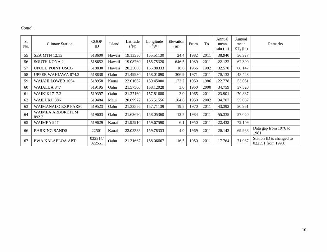
3.2.1 Rainfall
The rainfall databases available to IWREDSS across Hawaii’s islands are of different
periods of record (Table 3). The minimum period of record of the selected stations is of
19years, several stations have records of more than 50 years.
Short-duration missing rainfall data for a give station were estimated following
the normal ratio method that uses three index gauges which have the highest correlation
with the station in question. The analysis was carried out for each island individually and
all islands combined. There were minimal differences between general statistics of
complete data (mean, max, min, standard deviation) generated based on each island
individually and data of all islands combined; thus, data based on island wide analysis
was used to fill in the missing data.
Fig. 1 shows the comparison of annual average rainfall based on the observed data
of each station in the database and the value of rainfall grid of the corresponding station
derived from the Rainfall Atlas of Hawaii (Giambelluca et al., 2012).
R² = 0.9846
0
50
100
150
200
250
0 50 100 150 200 250
An
nu
al a
vera
ge r
ain
fall
-G
rid
val
ue
, R
ain
fall
Atl
as o
f H
awai
i
Annual average rainfall - Database, IWREDSS
1:1 Line
Linear Fit
Figure 1: Comparison of annual average rainfall (database, IWREDSS vs. grid value
derived from Rainfall Atlas of Hawaii, 2011).
3.2.2 Potential Evapotranspiration (ETo)
Reference evapotranspiration was calculated using Hargreaves-Samani (1982) equation

12
as detailed in Appendix 3. Minimum and Maximum temperature were used in
Hargreaves-Samani equation to calculate reference evapotranspiration. Missing
evapotranspiration data for any day was replaced with its daily average of all the other
years where there is data.
3.2.2.1 Adjustment of ETo
Daily ETo data generated with H-S equation were adjusted so that its average annual
value matches the average Pan Evaporation (PE) of the station as reported in Ekren and
Cheng (1985). Figure 2 shows a comparison of the annual average potential
evapotranspiration, ETo, of all stations calculated with H-S equation (adjusted) and
derived from (PE) data as reported by Ekren and Cheng (1985).
R² = 0.9834
0
20
40
60
80
0 20 40 60 80
An
nu
al a
vera
ge E
T o(B
ase
d o
n g
rid
va
lue
of
PE)
Annual average ETo - IWREDSS (Based on adjusted daily ETo
of the station)
1:1 Line
Linear Fit
Figure 2: Scatter plot of annual average ETo after adjustment of 56 stations based on PE
grid and 11 stations based on annual average PE of the station
3.3 Soil data
The updated soil survey dataset of the Island of Hawaii become available to the public in
September 2012 at the soil datamart (http://soildatamart.nrcs.usda.gov/ ). Soil data for
IWREDSS were updated incorporating updated soil data of the Island of Hawaii. Spatial
(Projected Coordinate System – NAD_1983_Zone_4N) and tabular data of the Island of

13
Hawaii and Hawaii Volcanoes National Park were collected from the webpage of the
Natural Resources Conservation Service (NRCS), United States Department of
Agriculture (USDA) (http://soildatamart.nrcs.usda.gov/Survey.aspx?State=HI).
Soil hydrologic group database of the Island of Hawaii was created using updated
soil data of Hawaii (i.e. HAWAII.csv). Similar database of all islands were combined to
create updated SOIL_HYDROGROUP.dbf.
3.4 GIS data
Details of all GIS layers included in IWREDSS are described in Appendix 1. Brief
description of updated GIS data is discussed here.
3.4.1 Soil data
The updated soil data of the Island of Hawaii was released to the public in September
2012 at the soil datamart (http://soildatamart.nrcs.usda.gov/ ); these soil data were used to
update IWREDSS 2.0 database. The spatial GIS data of the Island of Hawaii and Hawaii
Volcanoes National Park were downloaded from webpage of Natural Resources
Conservation Service (NRCS), United States Department of Agriculture (USDA).
3.4.2 TaxID
The updated TMK Parcels of all islands as of February 8, 2013 were downloaded from
the webpage of the Office of Planning, Department of Business, Economic Development
& Tourism, State of Hawaii (http://hawaii.gov/dbedt/gis/tmk.htm). The TMK Parcels of
all Islands were merged to create a new “TaxID” layer.
3.4.3 Soil Statistic dataset
The GIS layer of Soil statistics dataset, “TaxID_Soil” and dbf file,
“TaxID_Soil_Statistics.dbf” were updated using new data of soil and TaxID as explained
in Appendix 2 (Procedure for preparing Statistics dataset).
3.4.4 Rainfall grid
The updated Rainfall Atlas of Hawaii in Grid format (Giambelluca, 2012), was
downloaded from the web page of Geography Department, University of Hawaii at

14
Manoa (http://rainfall.geography.hawaii.edu/downloads.html). The updated rainfall grids
are based on the 30-year (1978-2007) mean. The size of grid is 250 × 250m.
3.4.5 Potential evaporation grid
The potential evaporation grid implement in IWREDSS is that produced by Ekren and
Cheng (1985). Their raster layer is used to scale evapotranspiration data of the nearest
weather station to the TMK of interest.
3.4.6 Climate stations
GIS data of climate stations were updated using coordinates and climate file name of all
the updated climate stations. Geographic Coordinates with 5 significant digits were used
for all stations in the database.
3.4.7 Aquifers
GIS data of the major Islands aquifers were downloaded from the webpage of Hawaii
Statewide Planning and Geographic Information System Program
(http://planning.hawaii.gov/gis/download-gis-data/). Aquifer boundaries of DLNR and
DOH were added to IWREDSS GIS data set library.
4. CALIBRATION AND VALIDATION
IWREDSS was calibrated and validated with data from the USDA-NRCS Handbook
Notice 38 that comprises net annual irrigation requirement maps for various crops grown
on the major islands of Hawaii. Several truck crops were selected (i. g., Egg Plant,
Tomato, Cabbage, Ginger, Dry Onion, Sweet Potato, and Watermelon). Irrigation
requirements were calculated for truck crops and banana at different islands assuming
under a drip irrigation system since it is the irrigation system of choice in Hawaii. Table 4
presents the calculated irrigation requirements by IWREDSS and a summary of their
corresponding estimates from the USDA-NRCS Handbook 38 (USDA-NRCS, 1996).
Percent differences between the two calculations were as low as 5% and varied as
a result of the crop type and location. The differences in the estimates were expected
since NRCS technique is more general and does not use specific crop parameters e.g.,
LAI, and SCS curve number information for different soil hydrological groups.

15
A regression analysis between the results of IWREDSS and the NRCS Handbook
38 was conducted (Fig. 3). Results show that there was a good agreement between the
two data sets (R2 = 0.83).
Table 4. Calibration and validation
Scenario Annual NIR (in) Variation
% Location, Crop, Irrigation System IWREDSS USDA-NRCS maps
Waimanalo (OA), Egg Plant, Trickle-Drip 23.1 17.0 36.1
Waimanalo (OA), Tomato, Trickle-Drip 24.2 17.0 42.3
Waimanalo (OA), Lettuce, Trickle-Drip 16.2 17.0 4.7
Waimanalo (OA), Cabbage, Trickle-Drip 19.1 17.0 12.6
Waianae (OA), Tomato, Trickle-Drip 49.1 59.0 16.8
Waianae (OA), Ginger, Trickle-Drip 55.6 59.0 5.7
Waianae (OA), Cabbage, Trickle-Drip 44.8 59.0 24.1
Waianae (OA), Egg Plant, Trickle-Drip 43.0 56.0 23.1
Waianae (OA), Dry Onion, Trickle-Drip 44.2 56.0 21.1
Kula (MA), Watermelon, Trickle-Drip 46.3 37.0 25.1
Kula (MA), Cabbage, Trickle-Drip 46.2 37.0 24.8
Kula (MA), Lettuce, Trickle-Drip 41.6 37.0 12.4
Haiku (MA), Banana (init), Trickle-Drip 31.2 42.5 26.7
Haiku (MA), Banana (init), Trickle-Drip 28.2 33.0 14.5
Haiku (MA), Banana (init), Trickle-Drip 25.5 30.0 15.1
Hoolehua (ML), Ginger, Trickle-Drip 50.8 55.0 7.6
Kaunakakai (ML), Ginger, Trickle-Drip 50.0 45.0 11.1
Kaunakakai (ML), Cabbage, Trickle-Drip 40.1 45.0 10.9
Kaunakakai (ML), Egg Plant, Trickle-Drip 42.2 45.0 6.3
Kilauea (KA), Egg Plant, Trickle-Drip 16.1 11.0 46.3
Kilauea (KA), Lettuce, Trickle-Drip 10.2 11.0 7.3
Kilauea (KA), Cabbage, Trickle-Drip 13.8 11.0 25.8

16
y = 1.0581xR² = 0.8305
0
15
30
45
60
0 15 30 45 60
USD
A-N
RC
S N
IR (
in)
IWREDSS NIR (in)
1:1 line
Figure 3: Validation of IWREDSS with USDA-NRCS results
5. PLOTTING THE MODEL RESULTS
The simulation results for all water budget components could be displayed with ArcGIS
software where all ArcGIS functions could be used on these output layers i.e., labeling,
classifying the parameters into various categories, merging or clipping more than one
layer, and/or application of field calculator to generate further data from the attribute
tables of the layers.
6. SENSITIVITY ANALYSIS
Sensitivity analysis is used to determine which input parameter has the greatest impact on
the model’s results/output. If a small change in a particular input parameter results in
relatively large changes in the output, the value of the input parameter is considered very
important and care should be given to accurately determine its values.
A Seed corn crop was selected for the sensitivity analysis because it became a
popular and an economically important crop in Hawaii. Table 5 shows some information
about seed corn, the average acreage of seed corn is 492 in the period between1999-2008
(National Agricultural Statistics Service, 2005, 2010) in Hawaii. The Trickle/drip

17
irrigation system was chosen due to its common use in Hawaii irrigated agriculture. The
water requirements/allocations were simulated for a four-month-growing season with
twelve different planting dates (from January to December). Since leaf area index (LAI)
is a function of the plant growth stage, an average LAI value of 2.0 was used for the
entire growing season. Water table depth was selected at 50 ft to consider deep water
table conditions. The values of these parameters were kept constant for all the
simulations; there were 12 simulations for windward (Waimanalo) and 12 simulations for
leeward (Kunia) sides of Oahu. Efforts were made to conduct simulations for a similar
soil type with the exact hydrological group (SCS curve number) to avoid soil type effect.
Hydrological groups of the soils at both locations were “B” and SCS curve numbers were
81. Annual average rainfall at Kunia was 27.2 in; whereas at Waimanalo it was 44.7 in.
Table 5. Sweet corn: Acreage, yield, production, price, and value, in Hawaii, 1999-2008. Year Acres Yield per acre Production Farm price
1,000 pounds Cents per pound
1999 450 3.8 1,700 58
2000 440 5.5 2,400 55
2001 440 4.3 1,900 64
2002 610 3.9 2,400 54
2003 830 3.0 2,500 51
2004 540 3.3 1,800 58
2005 410 4.1 1,700 55
2006 350 5.1 1,800 66
2007 450 5.3 2,400 62
2008 400 5.5 2,200 56

18
0
10
20
30
40
50
600
5
10
15
20
25
30
Jan
-A
pr
Feb
-M
ay
Mar
-Ju
n
Ap
r -J
ul
May
-A
ug
Jun
-Se
p
Jul -
Oct
Au
g -
No
v
Sep
-D
ec
Oct
-Ja
n
No
v -
Feb
De
c -
Mar
Gro
ss R
ain
fall
and
ETo
(in
)
NIR
(in
)
Assumed growing periods
Waimanalo (NIR) Kunia (NIR)
Waimanalo (Gross Rain) Kunia (Gross Rain)
Waimanalo (ETo) Kunia (ETo)
Figure 4. Changes in NIR based on changes in growing periods for seed corn grown on
windward (Waimanalo) and leeward (Kunia) sides of Oahu.
The results of the sensitivity analysis of growing periods and locations comprise
water budget components (Appendix 5a) and their corresponding statistics (Appendix
5b). The net irrigation requirements for the assumed growing periods are plotted in
Figure 4, which clearly depicts a significant difference in NIR for windward and leeward
sides of the island. The NIR were less during the wet period of the year (November to
April) and more during the dry months (May to October) regardless of the location on the
island.
6.1 Effect of crop leaf area index on irrigation allocations
For seed corn (growing season: April 15 to August 15), the NIR correlated positively with
effective rain (ER) and correlated negatively with leaf area index (Fig. 5. NIR increased
and ER decreased by almost 4% and 2%, respectively for every unit increase in the
average LAI (Fig.9).

19
y = 0.2143x + 8.7143R² = 0.9624
y = -0.24x + 6.3667R² = 0.9947
0
2
4
6
8
10
12
0 1 2 3 4 5
NIR
an
d E
R (
in)
Leaf Area Index
NIR ER
Fitted NIR Fitted ER
Figure 5: Net irrigation requirements (NIR) and effective rain (ER) versus leaf area index
(LAI)
y = -2.3292x + 5.2795R² = 0.9624
y = 4.0678x - 7.9096R² = 0.9947
-10
-5
0
5
10
15
0 1 2 3 4 5
% c
han
ge i
n N
IR a
nd
ER
Leaf Area Index
NIR ER
Fitted NIR Fitted ER
Figure 6. Percent change in Net irrigation requirements (NIR, open symbol) and effective
rain (ER, closed symbol) with leaf area index (LAI).
7. SIMULATION USING ENERGY CROPS
Energy crops included the family of crops that could be used to produce energy in forms
of heat or liquid fuel. Bioenergy crops often include food crops such as corn (starch for
ethanol production) and sugarcane (sugar for ethanol production). The water budget
components for the above energy crops were simulated for the dry and the wet growing
20
seasons for wind- and leeward sides of the island of Hawaii, Oahu, Maui and Kauai.
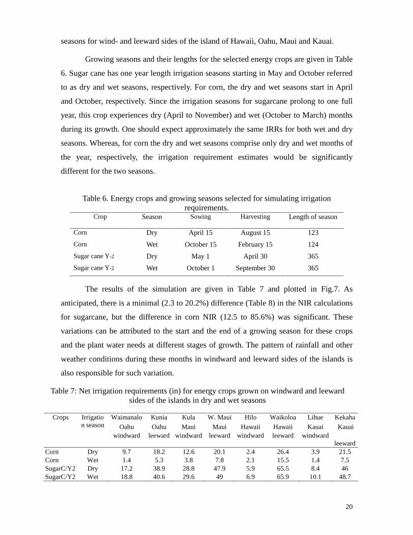
Growing seasons and their lengths for the selected energy crops are given in Table
6. Sugar cane has one year length irrigation seasons starting in May and October referred
to as dry and wet seasons, respectively. For corn, the dry and wet seasons start in April
and October, respectively. Since the irrigation seasons for sugarcane prolong to one full
year, this crop experiences dry (April to November) and wet (October to March) months
during its growth. One should expect approximately the same IRRs for both wet and dry
seasons. Whereas, for corn the dry and wet seasons comprise only dry and wet months of
the year, respectively, the irrigation requirement estimates would be significantly
different for the two seasons.
Table 6. Energy crops and growing seasons selected for simulating irrigation
requirements. Crop Season Sowing Harvesting Length of season
Corn Dry April 15 August 15 123
Corn Wet October 15 February 15 124
Sugar cane Y-2 Dry May 1 April 30 365
Sugar cane Y-2 Wet October 1 September 30 365
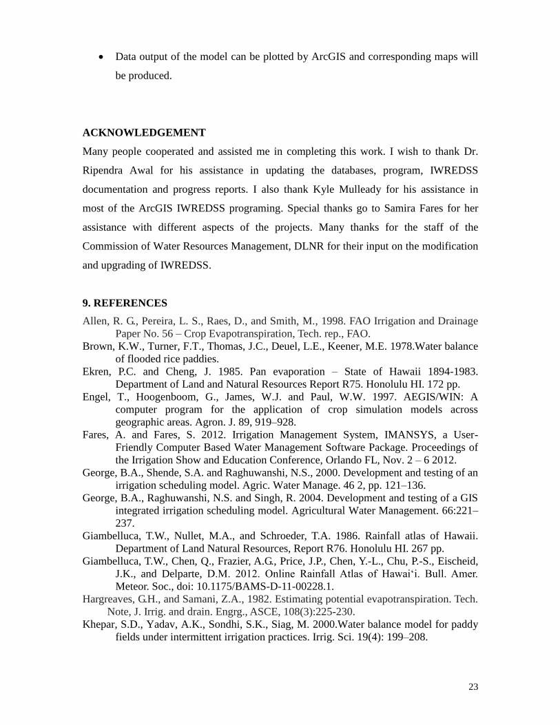
The results of the simulation are given in Table 7 and plotted in Fig.7. As
anticipated, there is a minimal (2.3 to 20.2%) difference (Table 8) in the NIR calculations
for sugarcane, but the difference in corn NIR (12.5 to 85.6%) was significant. These
variations can be attributed to the start and the end of a growing season for these crops
and the plant water needs at different stages of growth. The pattern of rainfall and other
weather conditions during these months in windward and leeward sides of the islands is
also responsible for such variation.
Table 7: Net irrigation requirements (in) for energy crops grown on windward and leeward
sides of the islands in dry and wet seasons
Crops Irrigatio
n season
Waimanalo Kunia Kula W. Maui Hilo Waikoloa Lihue Kekaha
Oahu Oahu Maui Maui Hawaii Hawaii Kauai Kauai
windward leeward windward leeward windward leeward windward
leeward
Corn Dry 9.7 18.2 12.6 20.1 2.4 26.4 3.9 21.5
Corn Wet 1.4 5.3 3.8 7.8 2.1 15.5 1.4 7.5
SugarC/Y2 Dry 17.2 38.9 28.8 47.9 5.9 65.5 8.4 46
SugarC/Y2 Wet 18.8 40.6 29.6 49 6.9 65.9 10.1 48.7

21
Table 8: Percent difference in the NIR calculated for energy crops during dry and wet
seasons
Crops Waimanalo Kunia Kula W. Maui Hilo Waikoloa Lihue Kekaha
Oahu Oahu Maui Maui Hawaii Hawaii Kauai Kauai
windward leeward windward leeward windward leeward windward leeward
Corn 85.6 70.9 69.8 61.2 12.5 41.3 64.1 65.1
Sugarcane 9.3 4.4 2.8 2.3 16.9 0.6 20.2 5.9
0
5
10
15
20
25
30
Oahu, W Oahu, L Maui, W Maui, L Hawaii, W Hawaii, L Kauai, W Kauai, L
NIR
(in
)
Dry Wet
(a) Corn
0
10
20
30
40
50
60
70
Oahu, W Oahu, L Maui, W Maui, L Hawaii, W Hawaii, L Kauai, W Kauai, L
NIR
(in
)
Dry Wet
Locations
(b) Sugarcane
Figure 7: Irrigation requirements for (a) corn and (b) sugarcane.

22
8. SUMMARY AND CONCLUSION
This is the final report for the project: “Water Management Software to Estimate Crop
Irrigation Requirements for Consumptive Use Permitting in Hawaii”. ArcGIS based
IWREDSS 2.0 was updated, calibrated, validated, and tested by conducting a sensitivity
analysis. The report presents and discusses results from calibration, validation and
sensitivity analysis. Hardware and software requirements are given in the IWREDSS 2.0
user manual (Appendix 1). Details on processes, governing equations, and methodologies
are given in the IWREDSS technical guide (Appendix 2).
IWREDSS was calibrated and validated for truck and energy crops based on the
data of the USDA-NRCS Handbook 38. A close agreement was observed between the
estimates of the two techniques. The sensitivity analysis revealed that IWREDSS results
are sensitive to the growing seasons due to variations in rainfall and ET. The LAI had
positive effect on NIR.
The new version of IWREDSS 2.0 is capable of calculating water budget
components for different crops grown on Hawaii. The current version, 2.0, comes with
the following features:
It estimates irrigation requirements for multiple crops/land uses, i.e., vegetable
and fruit crops, lawn and golf courses for different time intervals: daily, weekly,
bi-weekly, monthly, seasonally, and annually.
It uses long-term historical climate databases of daily ET and rain to calculate the
corresponding daily water budgets of the crop root zone. These calculations use a
long-term historical daily reference ET and rainfall for the locations of interest.
It estimates IRRs for different irrigation systems, including sprinkler, surface,
micro and seepage systems.
It uses specific inputs parameters for the crops, soils, irrigation systems, and
management factors. The user selects the values of these parameters; however,
default values are also included.
The model is flexible enough to allow the users to add more crops and/or update
data for a specific crop.
23
Data output of the model can be plotted by ArcGIS and corresponding maps will
be produced.
ACKNOWLEDGEMENT
Many people cooperated and assisted me in completing this work. I wish to thank Dr.
Ripendra Awal for his assistance in updating the databases, program, IWREDSS
documentation and progress reports. I also thank Kyle Mulleady for his assistance in
most of the ArcGIS IWREDSS programing. Special thanks go to Samira Fares for her
assistance with different aspects of the projects. Many thanks for the staff of the
Commission of Water Resources Management, DLNR for their input on the modification
and upgrading of IWREDSS.
9. REFERENCES
Allen, R. G., Pereira, L. S., Raes, D., and Smith, M., 1998. FAO Irrigation and Drainage
Paper No. 56 – Crop Evapotranspiration, Tech. rep., FAO.
Brown, K.W., Turner, F.T., Thomas, J.C., Deuel, L.E., Keener, M.E. 1978.Water balance
of flooded rice paddies.
Ekren, P.C. and Cheng, J. 1985. Pan evaporation – State of Hawaii 1894-1983.
Department of Land and Natural Resources Report R75. Honolulu HI. 172 pp.
Engel, T., Hoogenboom, G., James, W.J. and Paul, W.W. 1997. AEGIS/WIN: A
computer program for the application of crop simulation models across
geographic areas. Agron. J. 89, 919–928.
Fares, A. and Fares, S. 2012. Irrigation Management System, IMANSYS, a User-
Friendly Computer Based Water Management Software Package. Proceedings of
the Irrigation Show and Education Conference, Orlando FL, Nov. 2 – 6 2012.
George, B.A., Shende, S.A. and Raghuwanshi, N.S., 2000. Development and testing of an
irrigation scheduling model. Agric. Water Manage. 46 2, pp. 121–136.
George, B.A., Raghuwanshi, N.S. and Singh, R. 2004. Development and testing of a GIS
integrated irrigation scheduling model. Agricultural Water Management. 66:221–
237.
Giambelluca, T.W., Nullet, M.A., and Schroeder, T.A. 1986. Rainfall atlas of Hawaii.
Department of Land Natural Resources, Report R76. Honolulu HI. 267 pp.
Giambelluca, T.W., Chen, Q., Frazier, A.G., Price, J.P., Chen, Y.-L., Chu, P.-S., Eischeid,
J.K., and Delparte, D.M. 2012. Online Rainfall Atlas of Hawai‘i. Bull. Amer.
Meteor. Soc., doi: 10.1175/BAMS-D-11-00228.1.
Hargreaves, G.H., and Samani, Z.A., 1982. Estimating potential evapotranspiration. Tech.
Note, J. Irrig. and drain. Engrg., ASCE, 108(3):225-230.
Khepar, S.D., Yadav, A.K., Sondhi, S.K., Siag, M. 2000.Water balance model for paddy
fields under intermittent irrigation practices. Irrig. Sci. 19(4): 199–208.

24
Knox, J.W., Weatherhead, E.K., Bradley, R.I. 1997. Mapping the total volumetric
irrigation water requirements in England and Wales. Agric. Water Manage. 33
(1), 1–18.
Knox, J.W.,Weatherhead, E.K., Bradley, R.I. 1996. Mapping the spatial distribution of
volumetric irrigation water requirements for main crop potatoes in England and
Wales. Agric. Water Manage. 31(1–2):1–15.
Melaika, N.F. and Bottcher, A.B. 1988. Irrigation drainage management model for
Florida's Everglades Agricultural Area. American Society of Agricultural
Engineers Transactions 31(4): 1167–1172.
Mishra, A., 1999. Irrigation and drainage needs of transplanted rice in diked rice fields of
rainfed medium lands. Irrig. Sci. 19, 47–56.
National Agricultural Statistics Service. 2005. Statistics of Hawaii Agriculture 2003.
National Agricultural Statistics Service. 2010. Statistics of Hawaii Agriculture 2008.
www.nass.usda.gov/Statistics_by_State/Hawaii/Publications/Annual_Statistical_
Bulletin/all2008.pdf.
Odhiambo, L.O., Murty, V.V.N., 1996. Modeling water balance components in relation
to field layout in lowland paddy fields. II. Model application. Agric. Water
Manage. 30 (2), 201–216.
Pereira, L.A. 1989. Rice water management. Ph.D. Dissertation, ISA-UTL, Lisbon,
Portugal.
Paulo, A.M., Pereira L.A., Teixeira, J.L., Pereira, L.S. 1995. Modelling paddy irrigation.
In: Pereira L.S., vanden Broek, B.J., Kabat, P., Allen, R.G. (Eds.), Crop Water
Simulation Models in Practice. Wageningen Press, Wageningen, The Netherlands,
339 pp.
Samani, Z. 2000. Estimating solar radiation and evapotranspiration using minimum
climatological data. J Irrig Drain Engin. 126(4):265–267.
Satti, S.R. and Jacobs, J.M. 2004. A GIS-based model to estimate the regionally
distributed drought water demand. Agric. Wat. Manage. 66, pp. 1–13.
Satti, S.R., Jacobs, J.M and Irmak, S. 2004 Agricultural water management in a humid
region: sensitivity to climate, soil and crop parameters. Agricultural Water
Management. 70 (1) 51–65.
SCS. 1970. Irrigation Water Requirements. Technical Release No. 21. USDA Soil
Conservation Service. Washington, DC.
Shah, S.B., Edling, R.J. 2000. Daily evapotranspiration prediction from Louisiana
flooded rice field. J. Irrig. Drain. Eng. ASCE 126 (1), 8–13.
Smajstrla, A.G., Boman, B.J., Clark, G.A., Haman, D.Z., Izuno, F.T., and Zazueta. F.S.
1988a. Basic irrigation scheduling in Florida. Fla. Coop. Ext. Bull. 249.
Smajstrla, A. Zazueta, G., Parsons, D.S., and Stone, K.C. 1987. Trickle irrigation
scheduling for Florida citrus. Bull. 208. Florida Cooperative Extension Service,
IFAS, Univ. of Florida, Gainesville, FL.
Smajstrla, A.G. and Zazueta, F.S. 1987. Estimating Irrigation Requirements of Sprinkler
Irrigated Container Nurseries. Proc. Fla. State Hort. Soc., 100:343-348.
Smith, M., 1991. CROPWAT: a computer program for irrigation planning and
management. FAO Irrigation and Drainage Paper 46, FAO, Rome, Italy.
Stockle, C.O., Martin, S. and Campbell, G.S. 1994. CropSyst, a cropping systems model:
water/nitrogen budgets and crop yield. Agric. Syst. 46:335–359.
U.S. Census Bureau. 2002. Statistical abstract of the United States: 2002. U.S. Census
Bureau. Washington, DC.

25
USDA-NRCS. 1996. Handbook Notice # 38. Irrigation estimation maps for Hawaii.
Villalobos, F.J, and Fereres E. 1989. A simulation model for irrigation scheduling under
variable rainfall. Trans. ASAE 32(1):181-188.
Weatherhead, E.K., and Knox, J.W. 2000. Predicting and mapping the future demand for
irrigation water in England and Wales. Agric. Water Manage. 43(2): 203–218.
Young, C.A., and Wallender, W.W. 2002. Spatially distributed irrigation hydrology:
Water Balance. Trans. ASAE 45(3): 609–618.

26
10. APPENDICES
Appendix 1.
USER MANUAL
ArcGIS based graphical user interface of the Irrigation Water Requirement Estimation
Decision Support System (IWREDSS) enables users to calculate irrigation requirements
for given areas of their interest. Irrigation requirements can be calculated using either a
Tax-ID GIS layer or a geo-referenced map of the area. This manual includes the details
on how to digitize a hard copy of the area of interest. The user inputs include crop to be
grown/irrigated, crop leaf area index (LAI), the growing season, irrigation system to be
used, appropriate curve number, and water table depth. In addition to these inputs,
IWREDSS uses the corresponding weather and soil data from its Geo-databases.
IWREDSS results can be retrieved and visualized in the form of a text (ASCII) file and a
GIS map upon successful execution.
System Requirement
Hardware
The system is recommended to have at least 2GB of memory (RAM).
Software
IWREDSS was developed and tested on Windows XP, Windows 7 and 8 with installed
applications of ArcGIS 10.0 (ESRI product) and Java package - JRE (Java Runtime
Environment). JRE can be downloaded at http://www.oracle.com/technetwork/java/
javase/downloads/index.html. The following steps need to be completed to successfully
operate the program.
Installation of IWREDSS
1. Copy the parent folder entitled “IWREDSS” and all its contents to preferred location
on your computer (to your Desktop is fine). Do not alter the IWREDSS folder
structure in any way. The IWREDSS.mxd initiates ArcMap application of ArcGIS and
the data folder contains geo-databases of soil, climate, taxID, ALISH, LSB and an
executable file of IWREDSS engine IWREDSS.
2. Set system variable “IWREDSS_HOME” to be the location of IWREDSS (Figure 1).
To do this, click Start Menu > right-click Computer > click Properties > Advanced
Settings > Environment Variables. Under User Variables, click New. In the New

27
User Variable form, for Variable Name put IWREDSS_HOME. For Variable Value
put the path to where you placed the IWREDSS folder, e.g. C:\Documents and
Settings\Awal\Desktop\IWREDSS\. Make sure to include the IWREDSS folder in
the path name and to have a backslash at the end.
Figure 1
3. Install the IWREDSS ESRI Add-In and add the two IWREDSS buttons to ArcMap.
Open the IWREDSS folder and double-click IWREDSS.ESRIADDIN. When the
prompt window appears, click Install Add-In. This lets ArcGIS know that the add-in
exists. Now double-click IWREDSS.mxd. This will open ArcMap. When it opens,
click Customize > Customize Mode > Commands tab. In the Categories list, click
.NET Commands. You’ll see the two IWREDSS buttons in the Commands list. Drag
and drop both buttons onto a toolbar at the top of the ArcMap window.
Simulation using IWREDSS
Water budget components are simulated using various ways. IWREDSS provides an
option for Island wide and specific area simulation. Area simulation can be conducted by
selecting a TaxID area on any of the islands or by providing a user geo-referenced GIS
layer.

28
Area simulation using TaxID
Step 1: Open the ArcMap document
Open the file “IWREDSS.mxd” by double- or by right-clicking. An alternative way is to
launch ArcMap first, then open the document “IWREDSS.mxd” from the File->Open
menu or from ArcMap dialog, click the option to start using ArcMap with an existing
map, then click OK to browse for IWREDSS.mxd file. The document opens displaying a
map of Hawaii with polygons of different Tax ID areas (Figure 2).
Figure 2
The table of content (TOC) of ArcMap (a list on the left side of the window) includes the
following visible layers:
LSB: Land Study Bureau. (not active)
ALISH: Agricultural Lands of Importance to the State of Hawaii. (not active)
TaxID: The TaxID areas of all the islands
Station: The climate stations whose historical daily rainfall and ETo data are used by
IWREDSS.
Rain: Raster layer of rainfall. It contains annual average precipitation of every pixel on
the map. The values are calculated from the rainfall isohyets (Giambelluca, et al.,

29
2012). This layer is unselected by default.
ET: Raster layer of pan evaporation which contains annual average Pan Evaporation of
every pixel on the map. The values are calculated from the PE contours (Ekren and
Cheng, 1985). This layer is unselected by default.
SOILS: A soil layer presenting soils of Hawaii used in simulation.
The above layers may be at different order in TOC.
Step 2: Select a TaxID area
Locate the area of interest on one of the Hawaiian Islands. It is suggested to zoom in the
island of interest and click on TaxtID (irregular shaped polygons, sections on the map)
specific to the area of interest. There are two ways to select a TaxID area as follows:
1. Directly select on the map.
a) Using Zoom-in tool find the area to be irrigated/simulated.
b) Using Feature-selection tool select an area as shown in Figure 3. Note that
you can choose 1 area (TaxID) for simulation at a time.
Figure 3

30
2. Select by area from the attribute table (Figure 4).
a) In TOC, right click on TaxID and choose “Open Attribute Table” from the pop-up
menu.
b) In the attribute table, select Options->Select by Attribute, and then you can search
by TMK or other features (like all areas larger than 300,000 acres)
c) After clicking “apply”, the matched record(s) and area(s) will be highlighted. If
there are more than one records matched, you need to select only one from them.
d) Select TMK number chosen for simulation.
Figure 4
Step 3: Set other input parameters
After selecting an area, the user will need to input other required parameters by clicking
the IWREDSS tool button . The following window (Figure 5) will pop up.
User will need to input/select the following parameters:
Crop: User can select from the predefined list of crops given below:
27 PERENNIAL CROPS
GENERIC CROP

31
AVOCADO
BERMUDA GRASS
BREADFRUIT
CITRUS
COCONUT,PALMS
COFFEE
DENDROB.,POT
DILLIS GRASS
DOMEST.GARDEN
DRACEANE,POT
EUCALYP.,OLD
EUCALYP.,YNG
GARDEN HERBS
GUAVA
HELICONIA
KIKUYU GRASS
KOA
LYCHEE
MACADAMIA
MANGO
PAPAYA
ST.AUGUSTINA
TI
TURF, GOLF
TURF, LANDSCP
ZOYSIA GRASS
28 ANNUAL CROPS GENERIC CROP
ALFALFA,INIT
ALFALFA,RATN
BANANA,INIT
BANANA,RATN
CABBAGE
CANTALOUPE
DRY ONION
EGG PLANT
GINGER,(AWD)
LETTUCE
OTHER MELON
PEANUTS
PEPPERS
PINEAPP.YR-1
PINEAPP.YR-2
PUMPKIN
SEED CORN
SOYBEAN
SUGAR C.RATN
SUGAR C.YR-1
SUGAR C.YR-2
SUNFLOWERS
SWEET POTATO
TARO (Dry)
TARO (Wet)
TOMATO
Figure 5: Interface of IWREDSS
Figure 5: Interface of IWREDSS

32
WATER MELON
For each crop type, different root zone depths and water use coefficient data are
defined: for perennial crops, the parameters include irrigate crop zone depth, total zone
depth, monthly crop water use coefficient (KC), and monthly allowable water depletion
(AWD). For annual crops, the parameters include initial crop zone depth, maximum crop
zone depth, fraction of growth of 4 stages, crop water use coefficient (KC) of 4 stages, and
allowable water depletion (AWD) of 4 stages.
For simplicity, the utility of customize crop is not provided in IWREDSS.
Max LAI: Maximum Leaf Area Index; The parameter used to calculate interception.
Irrigation period: User can specify this period that can be up to 1 year long; it can start
at any month of the year and go around to the next year, i.e. starting date October of
year one and ending date November of the following year. Note that if the irrigation
period is too short (less than 45 days) for some annual crops, the simulation results
would not be accurate.
Irrigation system: The users can select from the predefined list of irrigation systems
given below:
USER-SPECIFIED SYSTEM
TRICKLE, DRIP
TRICKLE, SPRAY
MULTIPLE SPRINKLERS
SPRINKLER, CONTAINER NURSERY
SPRINKLER, LARGE GUNS
SEEPAGE, SUBIRRIGATION
CROWN FLOOD
FLOOD (TARO)
For an irrigation system different from those mentioned above, the predefined
parameters are different. The parameters include: system application efficiency,
fraction of soil surface irrigated, and fraction of evapotranspiration.
Option for no irrigation: A provision is given to calculate water budget components
without supplying additional irrigation. This option could be used for research
purpose as to consider a natural hydrologic cycle where only rainfall is the input
parameter and calculations are needed regarding effective rainfall,
evapotranspiration, canopy interception, runoff, and drainage of the conservation

33
lands or other areas of interest.
Irrigation practice: The users are given options to select irrigation practice. A dropdown
menu provides options for irrigation practices including a) Irrigate to field capacity
(normal practice); b) Apply a fixed depth per irrigation, and c) Deficit irrigation. In
case option “b” is selected, the users are asked to enter the depth of irrigation in
inches. Percentage of deficit irrigation is required to enter in case option “c” is
selected.
Additional Parameters: For the following list of the irrigation systems, additional
parameters are needed.
IR System Extra parameters
Crown Flood System Crown flood System bed height
Seepage System Depth to water table
Flood System Rice flood storage depth
The additional parameters (in inches) can be entered in a box provided next to the
Irrigation System box. When extra parameters are not needed, this box is grayed
out.
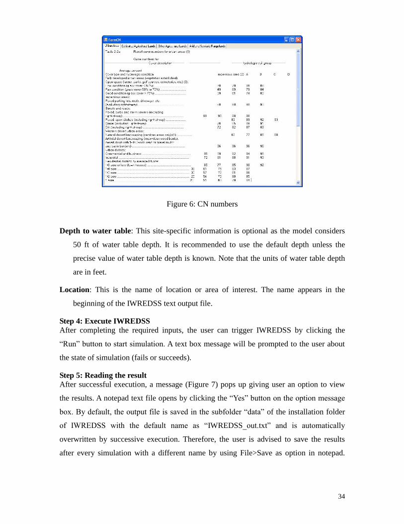
Soil Hydrological Groups and SCS Curve Numbers: All soil types in the selected
TaxID area are grouped into four hydrologic groups (A, B, C, and D). The portion of
each group of the soils in the selected area is given (for example, a selected area may
have 11.3% of group B, 22.8% of group C, and 64.8% of group D). For each group,
user has to specify the corresponding SCS curve number (CN) for all the soil types in
that group. The curve number is used in the calculation of runoff. For details of the
calculation, please refer to IWREDSS User Guide.
By default, a CN value of 78 is given for each hydrologic group to remind users that
they need to change these values to their correct values. Moreover, CN value of 78 is
representative of most grass covers. A list of CN values for different cover and soil
types is provided in Figure 6. User can refer to this list by clicking the “?” button
next to the CN input box.
34
Figure 6: CN numbers
Depth to water table: This site-specific information is optional as the model considers
50 ft of water table depth. It is recommended to use the default depth unless the
precise value of water table depth is known. Note that the units of water table depth
are in feet.
Location: This is the name of location or area of interest. The name appears in the
beginning of the IWREDSS text output file.
Step 4: Execute IWREDSS
After completing the required inputs, the user can trigger IWREDSS by clicking the
“Run” button to start simulation. A text box message will be prompted to the user about
the state of simulation (fails or succeeds).
Step 5: Reading the result
After successful execution, a message (Figure 7) pops up giving user an option to view
the results. A notepad text file opens by clicking the “Yes” button on the option message
box. By default, the output file is saved in the subfolder “data” of the installation folder
of IWREDSS with the default name as “IWREDSS_out.txt” and is automatically
overwritten by successive execution. Therefore, the user is advised to save the results
after every simulation with a different name by using File>Save as option in notepad.

35
Figure 7
The output text file contains three major sections: a legend table, simulation
parameters and simulation results. The legend table defines the abbreviations of
parameters used in the output and their corresponding units. These parameters include the
inputs parameters described in step 3 and the predefined parameters for crop type,
irrigation system, soil type, etc. The simulation results include the simulation result of
yearly average, monthly average, bi-weekly average and weekly average.
At the end of the output file, there is a summary of the results. Actually, the
simulation of IWREDSS is based on one soil type. Thus, if there is more than one soil
type for a particular area (or TaxID), IWREDSS would calculate irrigation requirements
for each of these soils independently. The total irrigation requirements for the area of
interest will be the weighted average of all the soils available in that area using the
following formula:
IRR = IRR1 * A1 / AT + IRR2 A2 / AT + … + IRRn * An / AT
where IRRi , Ai are the calculated irrigation requirements and the area occupied by i-th
soil respectively; AT is the total area of the different soils available in the total area of the
TaxID of interest. Note that IWREDSS will not simulate irrigation requirements for the
non-arable parts of the area of the TaxID; thus, the sum of the sums of all A’s will not be
equal if there are non-arable part of the area of interest. In these cases, the proportion will
be normalized so as to add up to 1. The list of all the simulated soil types and
corresponding proportion of each of them are given in the beginning of the summary
section of the report.
Summary of IWREDSS results are available at the end of the output file (Figure
8). IWREDSS uses calculated long-term daily record of irrigation water requirements to
calculate statistical parameters and probabilities of occurrence of IRRs for various time
periods (i.e., weekly, bi-weekly, monthly and yearly). Summary of IWREDSS results

36
provides IRRs for different probability levels, e.g. 50% (2 year return period), 80% (5
year return period), 90% (10 year return period) and 95% (20 year return period)
probability of GIRs. The 80% probability level (1 in 5 year return period) is
recommended by USDA-NRCS and is also used by the irrigation industry when
designing irrigation systems; thus, it was adopted for crop water allocation. The summary
table also provides information about irrigation season, irrigation system, climate
database, TMK, soil data and other parameters used.
Figure 8
Step 6: Plotting the result
Switching from the text output file to ArcMap .The user is prompted to plot the results
(Figure 9). The results are plotted on the map based on the yearly irrigation requirements
for different soil type in the TaxID area.

37
Figure 9
An example of color plotting is given in Figure 10. The user can visualize the results on
an enhanced option (Figure 11) by clicking the button to zoom to the whole TaxID
Area.
Figure 10

38
Figure 11
Simulation of user’s provided layer
Simulation of an actual location and net acres on a parcel can be conducted by using a
layer provided by the user. Ideally user’s layer should be a geo-referenced GIS layer. In
case user’s layer is in the shape of a parcel or a farm map, it needs to be digitized, geo-
referenced, saved as a polygon shapefile and have attribute table containing fields
including FID, SHAPE, ID, ISLAND. Stepwise procedure on how to digitize from a
parcel map is referred in the Technical Guide of IWREDSS.
The irrigation requirements for a user’s specified GIS layer can be simulated using two
methods. The user needs to provide a Geo-referenced GIS boundary layer of the area of
interest e.g. an agricultural field or a golf course. Method 1 is used to simulate user
defined layer when the area of interest is different from the combination of multiple
TMKs. Method 2 is used to simulate user defined layer when the area of interest is the
combination of multiple TMKs as a single polygon.
Method 1.
1. Add the folder containing supporting files of Geo-referenced GIS user’s layer in

39
“IWREDSS\data\GIS”
2. Create a folder “XXX_Soil (e.g. UserL_Soil)” in IWREDSS\data\GIS, where
XXX is the name of user’s layer (e.g. UserL). The name of the folder is case sensitive.
3. Add user’s layer in ArcMap TOC from “IWREDSS\data\GIS\folder containing
layer” (e.g. UserL).
4. The attribute table of the layer must contain fields including FID, Shape, Id,
ISLAND, and AREA. The AREA field should have data “Type” as “double”. The
ISLAND filed should have data “Type” as “Text” and “Length” equivalent to 10.
5. Values for the AREA field can be calculated using either VBScript or Python in
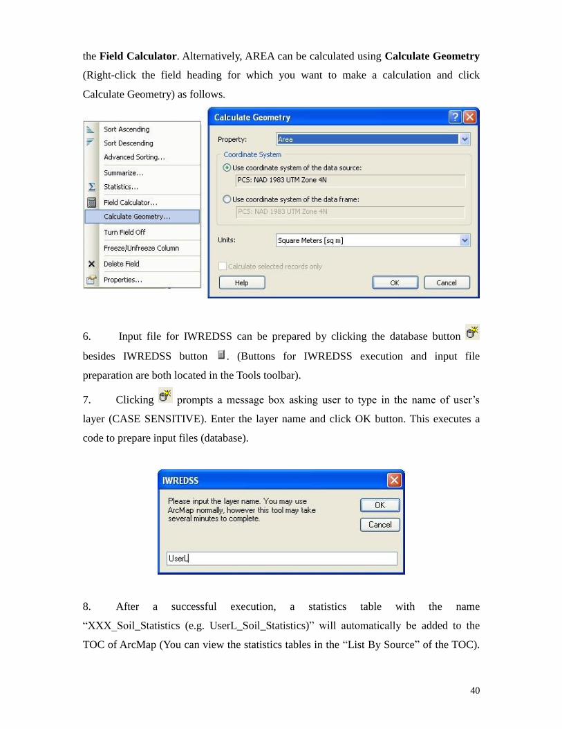
40
the Field Calculator. Alternatively, AREA can be calculated using Calculate Geometry
(Right-click the field heading for which you want to make a calculation and click
Calculate Geometry) as follows.
6. Input file for IWREDSS can be prepared by clicking the database button
besides IWREDSS button . (Buttons for IWREDSS execution and input file
preparation are both located in the Tools toolbar).
7. Clicking prompts a message box asking user to type in the name of user’s
layer (CASE SENSITIVE). Enter the layer name and click OK button. This executes a
code to prepare input files (database).
8. After a successful execution, a statistics table with the name
“XXX_Soil_Statistics (e.g. UserL_Soil_Statistics)” will automatically be added to the
TOC of ArcMap (You can view the statistics tables in the “List By Source” of the TOC).

41
Following message box will inform you after completion of data preparation:
9. Selecting user’s layer (e.g. UserL) and clicking IWREDSS button brings an
interface that requires input parameter selections (Don’t select other polygons in other
layers, just select polygon of user’s layer).
10. From dropdown menus select the name of Island and the name of the user’s layer
(case sensitive). (Complete Steps 3 through 6 i.e., complete the other input parameter
selections. Hit “Run” to start simulation, “Yes” to continue, “Yes” to see text simulation
results, and “Yes“ to plot the simulation results.

42
Method 2.
1. Select TMKs of TaxID which you want to make a single polygon (In this
example, TMKs 41026001, 41026002, 41026004 and 4126021 were selected).
2. Create new shape file (e.g. WUH1) from selected TMKs (Select TaxID at TOC >
Right click > Data > Export data)

43
3. Delete all fields in the attribute table of the new shape file (e.g. WUH1) except
FID, Shape, Area and ISLAND.

44
4. Create a new shape file (e.g. WUH) of a single polygon using Dissolve tool
(Geoprocessing > Dissolve) as shown in the following figure.
5. Add field ID in the attribute table of the dissolved new shape file (e.g. WUH). ID
should have data “Type” as “Integer” and “Precision” equal to 0.
6. Update AREA field in the attribute table of the new shape file.

45
7. Repeat steps 7 – 10 of the Method 1 to generate soil statistics table and to
simulate the area of interest (single polygon dissolved from multiple TMKs) as shown in
the following figure (The name of the folder (e.g. WUH) and the shape file (e.g. WUH)
should be the same. The shape file should be located at
C:../IWREDSS/Data/GIS/WUH/WUH).

46
Appendix 2.
TECHNICAL GUIDE
GeoDatabases, datasets and layers Beside the visible layers in the table of contents of ArcMAP, following datasets are also
included in the IWREDSS package:
TaxID_Soil_Statistics: The dBase dataset which have the intersection results of TaxID
layer and Soil Layer. Note in order to calculate efficiently, the original
intersection is summed by TaxID polygon and soil type so that there will be only
one record for each soil type in one TaxID area. .
Alish_Soil_Statistics: The dBase dataset which have the intersection results of Alish
layer and Soil Layer. Note in order to calculate efficiently, the original
intersection is summed by Alish polygon and soil type so that there will be only
one record for each soil type in one Alish area. .
LSB_Soil_Statistics: The dBase dataset which have the intersection results of LSB layer
and Soil Layer. Only type A, B, C, and D in LSB areas are included (type E is
conservation lands). Note in order to calculate efficiently, the original
intersection is summed by LSB polygon and soil type so that there will be only
one record for each soil type in one LSB area. .
User’s provided layer: There could be other layers for simulation and the corresponding
intersection layer (with soil) and statistic dataset should also be named as
XXX_Soil and XXX_Soil_Statistics. (XXX is the layer name).
IWREDSS Mechanism Area simulation
Upon user’s clicking on the IWREDSS tools button , the following data collection
process is launched:
1) Get the user’s selection; make sure there is one and only one area (of all layers)
selected; get the name of the layer the selection belongs to.
2) Query the statistic dataset described above (the datasets of the layer the selected area
belongs to) to get all the soil types and corresponding proportions and hydrologic
groups inside the selected area; note that non-arable soil types such as water, quarry

47
and so on will be filtered out before sending to IWREDSS for simulation, and soil
types that are of less than 1% of the whole area will not be simulated; get the
summation of each hydrologic group for user’s reference of CN specification later.
3) Find the geographically closest climate station (from the station layer) to the centroid
of the selected area; use the raster layers Rain and ET to get the annual average
rainfall and evapotranspiration of the closest station and those of the centroid of the
selected area so as to get the approximate ratios of rain and ET between the station
and the area. These ratios will be applied to the historic daily climate records of the
climate station during the simulation:
Rain_of_the_area = Rain_Ratio * Rain_of_Station
ET_of_the_area = ET_Ratio * ET_of_Station
The ratios are also shown on the parameter window.
4) Open the dialog to accept user’s input; assign the CN of each hydrologic group to all
the soil types of that group; launch IWREDSS; get results summary from IWREDSS
log; prompt error if fails, or confirmation if succeeds.
Data Plotting
After a successful execution, plotting is done upon request. The followings explain how it
is done by the VBA code.
1. Area simulation (XXX is the name of layer the selected area belongs to)
1) Add the intersection layer of the simulated area to the map, i.e.
data/GIS/XXX_Soil/XXX _Soil;
2) Select all the features (polygons) within the simulated area (the records with
FID_XXX = FID of the simulated area).
3) Output the selected features to IRR_PLOT_NNN_TT, where NNN is the island name
and TT is the current time of the plotting;
4) Add fields to the attribute table of the output layer, one for each of the water
components, and set the values to the IWREDSS results
5) Plot based on GIR field using natural breaks.
6) Remove the added and unused intersection layer.

48
2. Island simulation (XXX is the name of layer for the simulation)
Similar to area simulation, with the following differences:
1) The plotting is for the whole island, and the unit is area instead of soil polygons
within each area
2) The plotting is based on the summarized GIR (Gross Irrigation Requirement) values
of each area and the user can manually plot on any other water component.
3) The exported layer includes all areas of the selected island, while some of the areas
are not simulated because of non-arability. These un-simulated areas will have value 0
for all water component fields (displayed as white in the plotting).
Procedure for preparing Statistics dataset
This procedure works behind the input files preparation button provided besides
IWREDSS simulation button . The following description is for TaxID-related
simulations. The procedure for the other layers (ALISH, LSB, etc.) is mostly the same.
The TaxID layers are obtained from Hawaii State GIS Program
(http://www.hawaii.gov/dbedt/gis) and the soil layers are provided by USDA. In case
there are changes in the TaxID area division or soil type coverage, the statistics dataset
may need to be reproduced. The following procedure can be followed:
1) Merge the layers to be one big layer: TaxID. The Merge tool in ArcToolBox (Data
Management > Tools > General > Merge) provided by ArcMap is suitable for this
task.
2) Rename the TaxID layer as TaxID. Put it in the data/GIS/TaxID folder. Add ISLAND
field and set values. Add area field in the TaxID layer and use the Calculate Geometry
dialog box to calculate area.

49
4) 3) Use the ArcTool Intersect (ArcToolbox > Analysis Tools > Overlay > Intersect) to
intersect the TaxID layer and the soil layer. Output the intersection layer as
data/GIS/TaxID_Soil/TaxID_Soil. Add field NewArea (Double, length 19) to be the
area of the intersected polygon and field Portion (Double, length 19) to be the
proportion of NewArea to Area (the field from TaxID layer): NewArea/Area. Add to
the TaxID layer field FID_TaxID (Long integer, length 9) and set its value to be same
as field FID.
5) Add the field TaxID_SOIL (Text, length 20) in the intersect layer. Calculate the field
value as:
"" & [FID_TaxID] & "_" & [SOIL_CODE]
The field FID_TaxID is the FID field from TaxID layer which is automatically
renamed so during the intersection.
6) Use the ArcTool Summary Statistics (Analysis Tools > Statistics > Summary
Statistics) to generate the statistic dataset. The summary should be based on

50
TaxID_SOIL and output FID_TaxID, TMK, ISLAND, SOIL_CODE, NewArea, and
Portion. The first four fields can be summarized by first or last while the last two
fields must be summed. Output the statistic layer as data/GIS/TaxID_Soil/
TaxID_Soil_Statistics. Note if for layer of other names, not only the layer name
should be changed to XXX_Soil_Statistics, but also the path should be changed:
data/GIS/XXX_Soil/ XXX_Soil_Statistics
7) Rename the field names of the summary dataset:
first_fid_tax -> FID_TaxID (Double)
first_tmk -> TMK (Double)
first_island -> ISLAND (Text, 10)
first_soil_code -> SOIL_CODE (Text, 20)
sum_newarea -> AREA (Double)

51
sum_portion -> PORTION (Double)
The renaming process can be done by first add a new field with the desired name and
then calculate that field value by assigning it with the old field, and finally delete the
old field.
8) Add a field IL_Soil (Text, length 20) in the statistic dataset with the following value:
[ISLAND] & "_" & [SOIL_CODE]
9) Add the data/GIS/Soil/SOIL_HYDROGROUP.dbf; join it to the statistic dataset using
IL_Soil <-> IL_Soil. Add a new field GROUP (Text, length 1) in the statistic dataset,
assign the field value to be the field HYDROLIC of SOIL_HYDROGROUP, then
delete the join and remove SOIL_HYDROGROUP as
SOIL_HYDROGROUP.HYDROLIC.

52
10) Recalculate field PORTION to make all portions that are larger than 1 to be 1.as:
o Open the attribute table
o "Search by Attribute": "Portion" > 1
o Switch from all records to selected records
o Right click on the portion field and choose "field calculator"
o In the input box, type in 1 and click ok.
11) Check and make sure the records with empty value of field GROUP are fine.
12) Remove the intersection layer (XXX_SOIL) because it will be added and removed
automatically to the ArcMap document by code.
Procedure for preparing Statistics dataset (for user’s layers)
This program is designed to be able to handle new layers for simulation. To do that, the
corresponding layer and dataset need to be prepared as described above. The most
important things to be careful about are: field names, path and layer names. After all
datasets are prepared with the correct name in the correct path, the user will be able to do
exactly the same simulating job as when using the existing three layers. Area simulation
is also doable by choosing the desired area and run. Currently, the database button
performs this task for a user’s layer.
IWREDSS-related data
All the other data files that haven’t been described are of IWREDSS’ use. For more
details, please refer to IWREDSS User Manual.
How to Digitize in ArcGIS 10.0
1. Scan the image (rainfall isohyets or pan evaporation (PE) isolines) and save it
with extension .img or .jpeg
2. Open ArcCatalog, right click in your project folder (where your files are located)
and click, go to “New”, and click “Shapefile”. In “Create New Shapefile” window name
the new shapefile and select “polyline” as feature type. Select a projection through the
“Edit” button under “Description box”. You are in Spatial Reference Properties dialog
box. Click “Select” button, double click “Geographic coordinate systems”, double click
“North America”, double click “NAD 1983.prj, click “Add” button, and Click “Ok” at

53
the end.
3. Open a new ArcMap session and add the scanned image (.img or .jpeg extensions)
and the newly created polyline shape file, (You will find this file in the folder you created
from ArcCatalog. You can also drag it from ArcCatalog and drop it in TOC of ArcMap).
Add an already coordinated/Geo-referenced layer (It could be the coast line layer of the
islands or any other layer which have at least three bench marks or proper boundary
resembling the scanned image). This layer will be named “reference layer” in the rest of
the document.
4. Select Toolbars from the “Customize” menu in ArcMap and click “Editor” to turn
on the Editor toolbar if it is not already opened.
5. From the “Customize” menu go to “Toolbars” and click “Geo-referencing” if it is
not already opened.
6. Click the image layer to initiate it. Click the dropdown button of “Geo-
referencing” and click “Fit to Display”. You will see the scanned image on screen.
7. Right click the reference layer (e.g. island coast layer) and select “Zoom to
Layer”. You should see both the layers (the scanned image and the reference layer) on
screen.
8. From “Geo-referencing” toolbar click on ‘Add Control Points”, the line with red
and green x as endpoints.
9. Click a bench mark (any corner of a park, building or boundary) on the image first
followed by another click on the reference layer.
10. Repeat step 9 at least three or preferably four times to obtain different bench
marks or until you see the two layers overlaid.
11. Right click the new shape file and open attribute table. Add a new field (“Add
Field”) from the “Table Options” button on the top left corner. While creating a new field,
select proper features of the filed i.e. string for “text” data and integer or double
(depending on the size of the data) “number” data. Text may be the name of Island and
number may be the amount of rainfall or PE.
12. Click the new shapefile to initiate it, and from the “Editor” toolbar select “Start

54
Editing”
13. Zoom to the feature to be digitized, and select appropriate “Construction Tools” to
digitize desired shape.
14. Choose from the following options to create and modify the new feature:
To create a polygon feature, left-click once in the Data Frame to start a new
polygon. Successive single left-clicks will create vertices. Double-click at the last
vertex to create a closed polygon.
If you are editing a point feature class, left-click to add a single point location.
If you are editing a line feature, left-click to start a new line and add vertices with
successive single left-clicks. End the line with a double left-click.
If you are in the middle of editing a line and realize that you want to make a
correction to a part of that line you have already completed, double-click to finish
the line segment. Then select the “Edit Tool” (the black arrow just to the right of
”Editor”). Use this tool to select a feature by double-clicking it, and move the
vertices individually.
Use the “Esc” key to get out of a particular step.
The Undo option can be quite helpful. To use it, press Ctrl-z; alternatively, from
the Edit menu, select Undo. If your polygon gets too complicated to fix, you can
use the Edit Tool to select it, and then delete it by pressing the Del key.
Note: You can pan and zoom while in the middle of digitizing a feature. Another handy
feature is the magnifier window. To open this, from the main ArcMap menu bar, from the
“Window” menu, select “Magnifier”. This allows you to have a separate window zoomed
into a portion of the main Data Frame. You can pan and zoom this window around your
Data Frame, which is a convenient way to follow the path of a long feature.
15. After the digitizing is complete, enter the information to the attribute table of the
shapefile. Right click shapefile; click “Open Attribute Table”
16. Once you have digitized all the features, to save your edits, from the Editor
toolbar, select “Save Edits” from Editor.

55
17. To stop editing, from the Editor toolbar, select “Stop Editing’ from Editor.
18. Save the shapefile and use it with its supporting files.
How to add new crops in the existing crop list
The IWREDSS model gives the option to add a new crop in the existing list of crops.
Users need to figure out if the crop to be added is annual or perennial. There are two sets
of crops in the existing list of 27 perennial and 28 annual crops. Detail on crop
parameters including effective rooting depths, crop coefficients (KC), duration of crop
cycle and their fractions, and allowable water depletion (AWD) for major annual and
perennial crops are given in Tables 1 and 2 of the project report.
To update the existing list of crops:
Open croplist.dat with Notepad from IWREDSS\data. The first line in the text
gives the number of perennial crops followed by the names of the crops in the
sequence these appear in the interface of the IWREDSS model as demonstrated in
the following figure.
Update the crop list with the exact number and the names of the crops to be
added.
Save the croplist.dat file before closing it
Open IWREDSS\data\crop.dat in Notepad. The first two lines in the text give the
number of perennial crops and root zone and water use coefficient data i.e., crop
name, crop depth (inches), KC, Fraction, and AWD. The list of crops and the
related coefficients should be updated following the example of the existing
information as shown in the following figure.

56

57
For perennial crops, the crop data occupy the two rows for a single crop. The two
root zone depths in the second line of the crop data are irrigated and total root
zone depth i.e., 24 and 48 inches for Generic Crop, respectively. The values of KC
and AWD for different months of the year are given in the first line after crop
name and second line after irrigated and total root zone depth, respectively. The
root depth data are considered as average data for Hawaii conditions. Details of
the data for perennial crops are given in Table 2 of the project report.
Leave one line space between perennial and the annual crop information.
Details on the data for annual crops can be found in Table 1 of the project report.
The entries in Table 1 and in the above screen shot are explained in the following
table:
Column entries Description
1st Minimum annual crop irrigated root zone depth. This depth is
usually irrigated in the beginning of crop season
2nd Maximum crop irrigated root zone depth. Crops obtain and
maintain this maximum depth during their growth stages.
Patterns of crop root zone development are shown in the
following figure (Case of Seed Corn).
3rd through 6th The values of KC at initial, mid, and late stages of crop.
7th through 10th These are fraction of crop growing season under the heading of
FRACTION. The data represent duration of crop growth stage
that varies for various crops.
11th through 14th The fraction of total AWD during the four stages of crop.
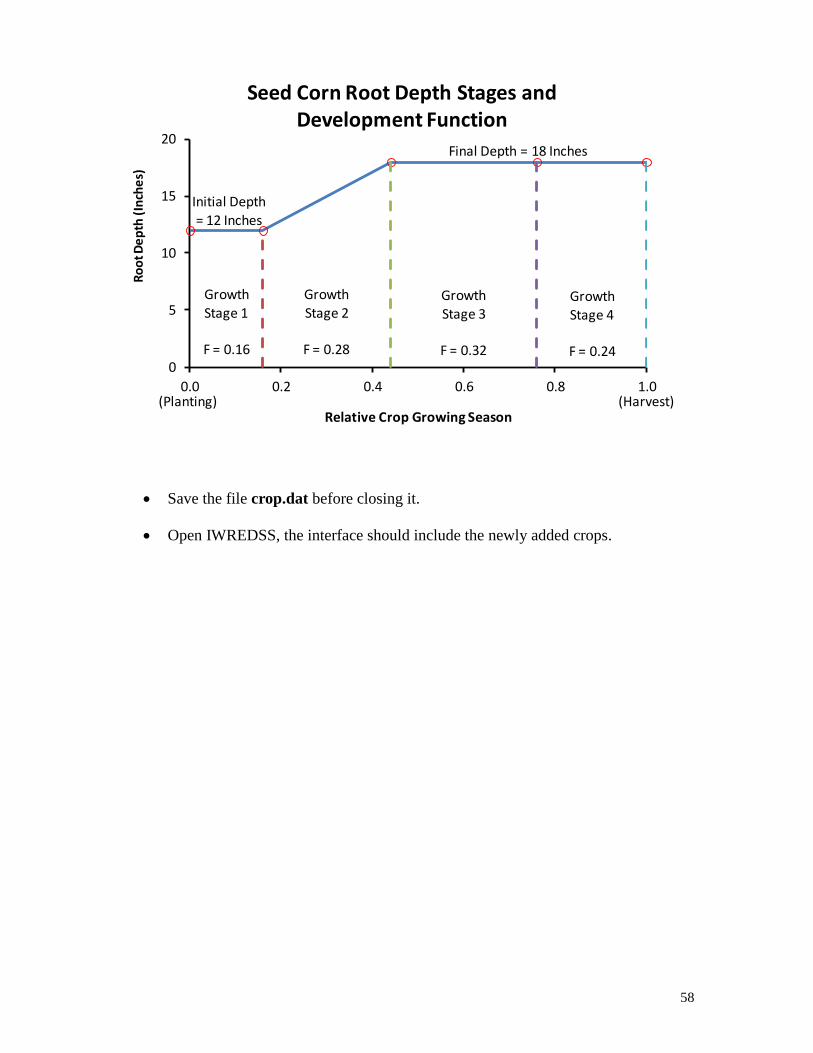
58
0
5
10
15
20
0.0 0.2 0.4 0.6 0.8 1.0
Ro
ot D
ep
th (
Inch
es)
Relative Crop Growing Season
Seed Corn Root Depth Stages and Development Function
Growth Stage 1
F = 0.16
Growth Stage 2
F = 0.28
Growth Stage 3
F = 0.32
Growth Stage 4
F = 0.24
Initial Depth
= 12 Inches
Final Depth = 18 Inches
(Planting) (Harvest)
Save the file crop.dat before closing it.
Open IWREDSS, the interface should include the newly added crops.

59
Appendix 3. Calculation of daily ETo using temperature data.
STEP 1: Extraterrestrial radiation (Ra) is calculated for each day using the following
equations from Duffie and Beckman (1980) (reproduced from Snyder and Eching, 2002).
STEP 2: Calculate ET using Hargreaves-Samani equation (Hargreaves and Samani, 1982)
(reproduced from Snyder and Eching, 2002).
where: Tm
= mean daily temperature in o
C, TX = the maximum daily air temperature in
o
C,
and Tn = the minimum daily air temperature in
o
C.
References:
Duffie, J.A. and Beckman, W.A. 1980. Solar engineering of thermal processes. John Wiley and Sons,
New York. pp. 1-109.
Hargreaves, G.H., and Samani, Z.A. 1982. Estimating potential evapotranspiration, Tech. Note, J.
Irrig. and drain. Eng., ASCE, 108(3):225-230.
Snyder, R.L, Eching, S. 2002. Penman-Monteith daily (24-hour) Reference Evapotranspiration
Equations for Estimating ETo, ETr and HS ETo with Daily Data. Regents of the University of
California.
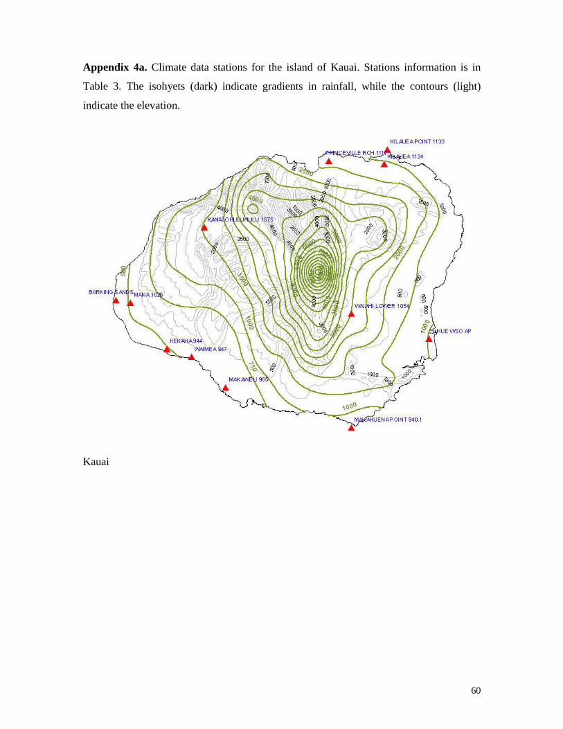
60
Appendix 4a. Climate data stations for the island of Kauai. Stations information is in
Table 3. The isohyets (dark) indicate gradients in rainfall, while the contours (light)
indicate the elevation.
Kauai
1

61
Appendix 4b. Climate data stations for the island of Oahu and Molokai. Stations
information is in Table 3. Isohyets (dark) indicate gradients in rainfall (dark). The
contours (light) indicate the elevation.
Oahu
Molokai
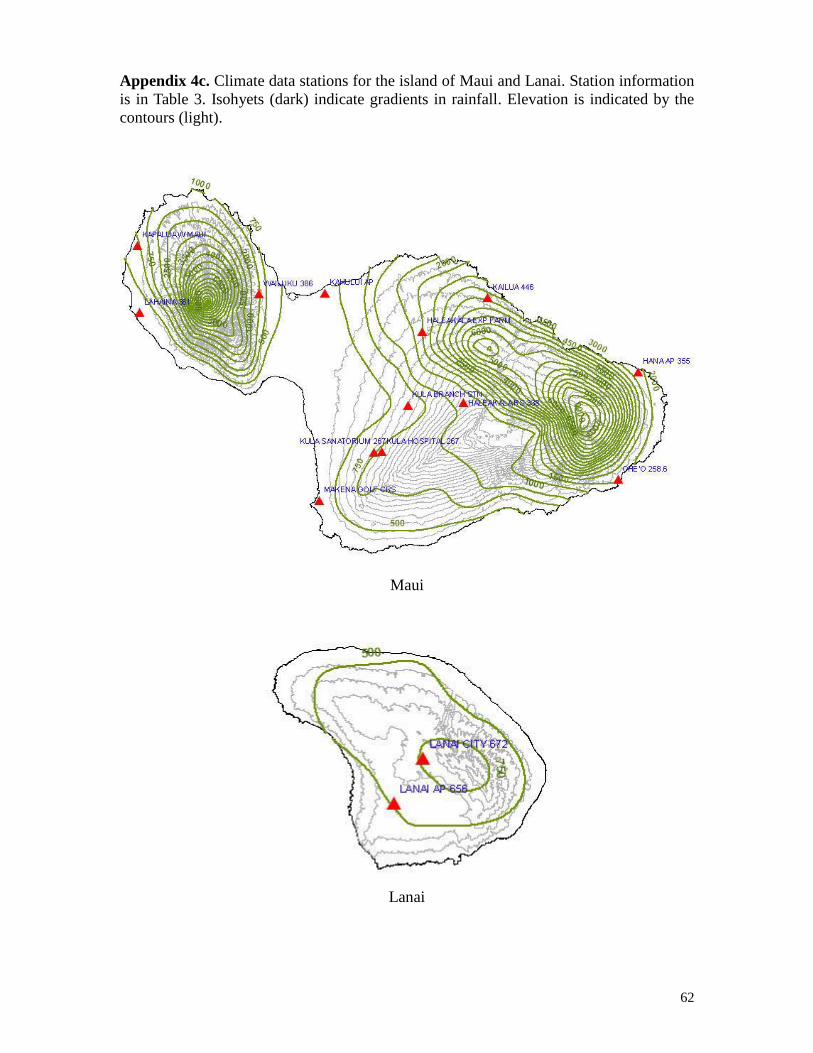
62
Appendix 4c. Climate data stations for the island of Maui and Lanai. Station information
is in Table 3. Isohyets (dark) indicate gradients in rainfall. Elevation is indicated by the
contours (light).
Maui
Lanai
11

63
Appendix 4d. Climate data stations for the island of Hawaii. Stations information is in
Table 3. Isohyets (dark) indicate gradients in rainfall. Elevation is indicated by the
contours (light).
Hawaii

64
Appendix: 5a: Seasonal water budget components
Seasonal (Jan - Apr) water budget components
MO NIR GIR GAL_A G_RAIN N_RAIN ER ER21 RO INT ETo ET DR
Jan 0 0 0 6.8 4.9 2.4 3.3 1.9 0 3.4 2.3 2.5
Feb 0.4 0.5 13.1 4.8 3.5 2.3 2.6 1.2 0.2 3.5 3.6 1.2
Mar 1.6 1.9 50.8 4.6 3.4 2.6 2.9 1 0.2 4.2 5.1 0.8
Apr 1.2 1.4 37.5 3.3 2.5 2.3 2.1 0.6 0.2 4.5 3.9 0.2
Jan - Apr 3.2 3.7 101.4 19.6 14.3 9.6 10.9 4.6 0.6 15.6 14.9 4.8
Seasonal (Feb - May) water budget components
MO NIR GIR GAL_A G_RAIN N_RAIN ER ER21 RO INT ETo ET DR
Feb 0 0 1.3 4.8 3.6 2 2.2 1.2 0 3.5 2.2 1.6
Mar 0.8 1 26.3 4.6 3.5 2.3 2.7 1 0.2 4.2 4.3 1.2
Apr 2 2.3 63.7 3.3 2.5 2.3 2.3 0.6 0.2 4.5 5.4 0.2
May 2 2.4 64.2 2.9 2.2 2.1 1.8 0.5 0.2 5 4.4 0.1
Feb - May 4.9 5.7 155.5 15.7 11.8 8.7 9.1 3.2 0.6 17.2 16.2 3.1
Seasonal (Mar - Jun) water budget components
MO NIR GIR GAL_A G_RAIN N_RAIN ER ER21 RO INT ETo ET DR
Mar 0.1 0.2 4.2 4.6 3.6 2.1 2.3 1 0 4.2 2.7 1.5
Apr 1.1 1.3 36.1 3.3 2.6 2.2 2.2 0.6 0.2 4.5 4.6 0.4
May 3 3.5 94.7 2.9 2.2 2 2 0.5 0.2 5 6 0.1
Jun 2.6 3.1 83.2 1.4 1 1 1 0.1 0.2 4.9 4.2 0
Mar - Jun 6.8 8 218.3 12.2 9.4 7.3 7.4 2.2 0.6 18.6 17.5 2.1
Seasonal (Apr - Jul) water budget components
MO NIR GIR GAL_A G_RAIN N_RAIN ER ER21 RO INT ETo ET DR
Apr 0.2 0.2 6 3.3 2.7 2 1.8 0.6 0 4.5 2.8 0.7
May 1.7 2 53.4 2.9 2.2 1.9 1.9 0.5 0.2 5 5.1 0.4
Jun 3.7 4.3 117.8 1.4 1 1 1 0.1 0.2 4.9 5.9 0
Jul 3 3.5 94.3 1.6 1.4 1.4 1.2 0 0.2 5.1 4.4 0
Apr - Jul 8.5 10 271.5 9.2 7.4 6.3 5.9 1.3 0.6 19.5 18.2 1.1
Seasonal (May - Aug) water budget components
MO NIR GIR GAL_A G_RAIN N_RAIN ER ER21 RO INT ETo ET DR
May 0.3 0.4 11 2.9 2.4 1.7 1.5 0.5 0 5 3 0.6
Jun 2.4 2.8 75.9 1.4 1.1 1.1 1 0.1 0.1 4.9 5 0
Jul 4 4.7 126.9 1.6 1.4 1.4 1.3 0 0.2 5.1 6.1 0
Aug 3 3.5 95.2 1.6 1.3 1.3 1.1 0.1 0.2 5.1 4.4 0
May - Aug 9.7 11.4 309 7.5 6.1 5.4 4.9 0.8 0.6 20.1 18.5 0.6

65
Seasonal (Jun - Sep) water budget components
MO NIR GIR GAL_A G_RAIN N_RAIN ER ER21 RO INT ETo ET DR
Jun 0.4 0.4 11.9 1.4 1.2 1.1 0.8 0.1 0 4.9 2.7 0.1
Jul 2.5 2.9 80 1.6 1.4 1.4 1.2 0 0.2 5.1 5.2 0
Aug 4 4.7 127.9 1.6 1.3 1.3 1.2 0.1 0.2 5.1 6.1 0
Sep 2.5 3 81.3 1.9 1.6 1.6 1.3 0.1 0.2 4.7 4.1 0
Jun - Sep 9.4 11.1 301 6.5 5.5 5.5 4.5 0.4 0.6 19.8 18.1 0.1
Seasonal (Jul - Oct) water budget components
MO NIR GIR GAL_A G_RAIN N_RAIN ER ER21 RO INT ETo ET DR
Jul 0.4 0.4 11.9 1.6 1.6 1.5 1 0 0 5.1 3 0
Aug 2.5 3 80.4 1.6 1.3 1.3 1.1 0.1 0.2 5.1 5.2 0
Sep 3.4 4 109.3 1.9 1.6 1.6 1.4 0.1 0.2 4.7 5.6 0
Oct 1.7 2.1 55.8 3.6 2.6 2.6 2.1 0.7 0.2 4.1 3.7 0.1
Jul - Oct 8.1 9.5 257.4 8.7 7.2 7 5.6 1 0.6 19 17.5 0.1
Seasonal (Aug - Nov) water budget components
MO NIR GIR GAL_A G_RAIN N_RAIN ER ER21 RO INT ETo ET DR
Aug 0.5 0.6 15.8 1.6 1.5 1.3 0.9 0.1 0 5.1 2.9 0.1
Sep 2.1 2.4 66.1 1.9 1.7 1.7 1.3 0.1 0.1 4.7 4.8 0
Oct 2.2 2.6 70.5 3.6 2.6 2.5 2.2 0.7 0.2 4.1 4.9 0.1
Nov 0.6 0.7 18.2 6.2 4.4 3.5 3.4 1.6 0.3 3.2 2.9 0.9
Aug - Nov 5.3 6.3 170.6 13.3 10.2 9.1 7.9 2.5 0.6 17.1 15.6 1.1
Seasonal (Sep - Dec) water budget components
MO NIR GIR GAL_A G_RAIN N_RAIN ER ER21 RO INT ETo ET DR
Sep 0.3 0.3 9 1.9 1.8 1.7 1.1 0.1 0 4.7 2.8 0.1
Oct 1.2 1.4 36.8 3.6 2.7 2.3 2.1 0.7 0.2 4.1 4.1 0.3
Nov 0.9 1 28.1 6.2 4.4 3.4 3.6 1.6 0.3 3.2 3.9 1
Dec 0.3 0.3 9.4 5.9 4.3 2.9 3.1 1.4 0.3 3.1 2.8 1.3
Sep - Dec 2.6 3.1 83.3 17.6 13.2 10.4 9.9 3.8 0.7 15.1 13.6 2.8
Seasonal (Oct - Jan) water budget components
MO NIR GIR GAL_A G_RAIN N_RAIN ER ER21 RO INT ETo ET DR
Oct 0.1 0.1 2.5 3.6 2.9 2.1 0.9 0.7 0 4.1 2.5 0.7
Nov 0.3 0.3 9.3 6.3 4.5 2.8 1.5 1.6 0.2 3.2 3.3 1.7
Dec 0.6 0.7 18.1 6 4.3 3 1.4 1.4 0.3 3.1 3.7 1.3
Jan 0.3 0.3 8.7 6.6 4.5 2.8 3 1.9 0.2 3.3 2.9 1.6
Oct - Jan 1.2 1.4 38 22.7 16.3 10.9 6.8 5.7 0.7 13.8 12.6 5.4

66
Seasonal (Nov - Feb) water budget components
MO NIR GIR GAL_A G_RAIN N_RAIN ER ER21 RO INT ETo ET DR
Nov 0 0 0 6.3 4.7 2.3 1.5 1.6 0 3.2 2.2 2.5
Dec 0.2 0.2 6.3 6 4.4 2.6 1.4 1.4 0.2 3.1 3.2 1.8
Jan 0.5 0.6 16.7 6.8 4.6 3.2 3 1.9 0.3 3.4 4.1 1.4
Feb 0.3 0.4 10.6 4.5 3.3 2.4 2.2 1 0.2 3.4 2.9 0.9
Nov - Feb 1.1 1.2 33.6 24 17.2 10.5 8.1 6.1 0.7 13.2 12.5 6.7
Seasonal (Dec - Mar) water budget components
MO NIR GIR GAL_A G_RAIN N_RAIN ER ER21 RO INT ETo ET DR
Dec 0 0 0.9 6 4.5 2.1 1.4 1.4 0 3.1 2.1 2.4
Jan 0.2 0.3 7.6 6.8 4.7 2.8 3 1.9 0.2 3.4 3.6 1.9
Feb 0.9 1.1 29.9 4.9 3.5 2.6 2.2 1.2 0.2 3.5 4.2 0.8
Mar 0.9 1 27.2 4.5 3.4 2.4 2.3 1 0.2 4.1 3.7 0.9
Dec - Mar 2 2.4 65.1 22.4 16.2 10 8.9 5.5 0.7 14.2 13.6 6.2
Appendix 5b: Statistics for seasonal gross and net irrigation requirements
Statistics for seasonal gross and net irrigation requirements (Jan - Apr)
MO MEAN MED. CV XMAX XMIN ZERO RSQ 50% 80% 90% 95%
Jan 0 0 0 0 0 0 1 0 0 0 0
Feb 0.5 0 1.35 2.7 0 0 0.73 0.6 1 1.4 1.7
Mar 1.9 1 0.83 4.9 0 0 0.89 1.5 3.1 4.3 5.3
Apr 1.4 1.2 0.78 3.8 0 0 0.81 1.5 2.3 2.8 3.2
NIR (Jan - Apr) 3.2 3.1 0.69 8.3 0 0 0.96 2.7 5.2 6.9 8.5
Statistics for seasonal gross and net irrigation requirements (Feb - May)
MO MEAN MED. CV XMAX XMIN ZERO RSQ 50% 80% 90% 95%
Feb 0 0 3.65 0.7 0 0 0 0 0 0 0
Mar 1 0.9 0.98 3.4 0 0 0.91 0.9 1.7 2.3 2.9
Apr 2.3 1.9 0.56 4.9 0 0 0.94 2.2 3.5 4.3 4.9
May 2.4 2.5 0.52 4.7 0 0 0.91 2.3 3.4 4.1 4.6
NIR (Feb - May) 4.9 4.8 0.46 9 0.8 0 0.97 4.6 7.1 8.5 9.7
Statistics for seasonal gross and net irrigation requirements (Mar - Jun)
MO MEAN MED. CV XMAX XMIN ZERO RSQ 50% 80% 90% 95%
Mar 0.2 0 1.81 0.7 0 0 0.95 0.6 0.6 0.7 0.7
Apr 1.3 0.9 0.78 3.5 0 0 0.87 1.2 2.1 2.7 3.3
May 3.5 3.8 0.4 5.8 0 0 0.93 3.4 4.8 5.5 6.1
Jun 3.1 3.1 0.39 5.1 0 0 0.89 3 4.1 4.7 4.9
NIR (Mar - Jun) 6.8 7 0.35 11.1 1.9 0 0.98 6.8 9.1 10.2 11.2

67
Statistics for seasonal gross and net irrigation requirements (Apr - Jul)
MO MEAN MED. CV XMAX XMIN ZERO RSQ 50% 80% 90% 95%
Apr 0.2 0 1.43 0.7 0 0 0.75 0.6 0.7 0.7 0.7
May 2 1.9 0.55 3.7 0 0 0.94 1.9 2.9 3.6 4.1
Jun 4.3 4.4 0.27 6.3 0.9 0 0.94 4.4 5.4 5.8 6.2
Jul 3.5 3.7 0.26 5.2 1.2 0 0.87 3.5 4.3 4.7 5
NIR (Apr - Jul) 8.5 9 0.25 12.8 3.4 0 0.99 8.6 10.5 11.4 12.2
Statistics for seasonal gross and net irrigation requirements (May - Aug)
MO MEAN MED. CV XMAX XMIN ZERO RSQ 50% 80% 90% 95%
May 0.4 0.6 0.94 1.3 0 0 0.64 0.6 0.7 0.8 0.9
Jun 2.8 2.8 0.38 4.6 0.8 0 0.93 2.7 3.8 4.4 4.9
Jul 4.7 4.9 0.21 6.1 2.8 0 0.95 4.7 5.6 6 6.3
Aug 3.5 3.7 0.27 5.1 1.3 0 0.85 3.5 4.4 4.8 5.2
NIR (May - Aug) 9.7 9.6 0.2 13.6 4.4 0 0.99 9.8 11.4 12.2 12.7
Statistics for seasonal gross and net irrigation requirements (Jun - Sep)
MO MEAN MED. CV XMAX XMIN ZERO RSQ 50% 80% 90% 95%
Jun 0.4 0.6 0.68 0.7 0 0 0.95 0.6 0.7 0.7 0.7
Jul 2.9 3.1 0.3 4.4 0.8 0 0.94 2.9 3.8 4.2 4.6
Aug 4.7 4.9 0.24 6.7 2.8 0 0.94 4.7 5.7 6.2 6.6
Sep 3 2.6 0.27 4 1.2 0 0.81 3 3.7 4 4.3
NIR (Jun - Sep) 9.4 9.4 0.21 13.3 4.9 0 0.99 9.5 11.2 12 12.6
Statistics for seasonal gross and net irrigation requirements (Jul - Oct)
MO MEAN MED. CV XMAX XMIN ZERO RSQ 50% 80% 90% 95%
Jul 0.4 0.6 0.93 1.4 0 0 0.63 0.6 0.8 0.9 1
Aug 3 3.1 0.35 4.5 0.8 0 0.91 2.9 4 4.6 5.1
Sep 4 3.9 0.24 6 2 0 0.92 4.1 4.8 5.2 5.5
Oct 2.1 2.3 0.56 4.7 0 0 0.9 2 3 3.6 4.1
NIR (Jul - Oct) 8.1 8.1 0.27 13.5 4 0 0.99 8.1 10 10.9 11.7
Statistics for seasonal gross and net irrigation requirements (Aug - Nov)
MO MEAN MED. CV XMAX XMIN ZERO RSQ 50% 80% 90% 95%
Aug 0.5 0.6 15.8 1.6 1.5 1.3 0.9 0.1 0 5.1 2.9
Sep 2.1 2.4 66.1 1.9 1.7 1.7 1.3 0.1 0.1 4.7 4.8
Oct 2.2 2.6 70.5 3.6 2.6 2.5 2.2 0.7 0.2 4.1 4.9
Nov 0.6 0.7 18.2 6.2 4.4 3.5 3.4 1.6 0.3 3.2 2.9
NIR (Aug - Nov) 5.3 5.6 0.36 9.3 1.5 0 0.99 5.3 7.1 8.1 8.9

68
Statistics for seasonal gross and net irrigation requirements (Sep - Dec)
MO MEAN MED. CV XMAX XMIN ZERO RSQ 50% 80% 90% 95%
Sep 0.3 0 1.15 1.4 0 0 0.53 0.5 0.7 0.8 0.9
Oct 1.4 1.3 0.74 3.5 0 0 0.92 1.3 2.2 2.8 3.4
Nov 1 0.9 0.99 2.9 0 0 0.88 1 1.9 2.5 3.1
Dec 0.3 0 1.6 1.3 0 0 0.87 1.1 1.2 1.2 1.2
NIR (Sep - Dec) 2.6 2.3 0.59 5.4 0 0 0.96 2.3 4.1 5.1 6.1
Statistics for seasonal gross and net irrigation requirements (Oct - Jan)
MO MEAN MED. CV XMAX XMIN ZERO RSQ 50% 80% 90% 95%
Oct 0.1 0 2.45 0.7 0 0 0.92 0.5 0.6 0.6 0.7
Nov 0.3 0 1.62 1.8 0 0 0.78 0.4 0.9 1.2 1.5
Dec 0.7 0.9 1.07 2 0 0 0.78 0.8 1.3 1.6 1.9
Jan 0.3 0 1.68 1.3 0 0 0.94 1.1 1.2 1.2 1.2
NIR (Oct - Jan) 1.2 0.8 0.94 4.2 0 0 0.92 1 2 2.7 3.4
Statistics for seasonal gross and net irrigation requirements (Nov - Feb)
MO MEAN MED. CV XMAX XMIN ZERO RSQ 50% 80% 90% 95%
Nov 0 0 0 0 0 0 1 0 0 0 0
Dec 0.2 0 1.68 0.9 0 0 0.61 0.7 0.8 0.9 0.9
Jan 0.6 0 1.21 2.8 0 0 0.78 0.7 1.2 1.6 2
Feb 0.4 0 1.94 2.5 0 0 0.78 0.4 1.1 1.6 2.1
NIR (Nov - Feb) 1.1 0.8 1.02 3.5 0 0 0.93 0.9 2 2.7 3.5
Statistics for seasonal gross and net irrigation requirements (Dec - Mar)
MO MEAN MED. CV XMAX XMIN ZERO RSQ 50% 80% 90% 95%
Dec 0 0 4.47 0.7 0 0 0 0 0 0 0
Jan 0.3 0 1.5 1 0 0 0.68 0.7 0.9 0.9 1
Feb 1.1 0.9 0.95 3.8 0 0 0.87 1 1.9 2.5 3.1
Mar 1 1 1.12 3.8 0 0 0.82 1.1 2 2.6 3.2
NIR (Dec - Mar) 2 1.6 0.87 6.2 0 0 0.94 1.5 3.4 4.8 6.1