debt servicing costs and capital structurejl3271/jmp_jeonghwanlee.pdf · debt servicing costs and...

Debt Servicing Costs and Capital Structure

Jeong Hwan Lee�

November 19, 2013Job Market Paper

Abstract

In contrast to the standard capital structure theory prediction that builds on a trade-o¤

between interest tax shields and expected bankruptcy costs, public �rms use debt quite

conservatively. To address this well known debt conservatism puzzle (Graham 2000), I

argue that servicing debt drains valuable liquidity for a �nancially constrained �rm and

hence endogenously creates �debt servicing costs,�which have received little attention in the

literature. To examine the in�uence of debt servicing costs on capital structure choices, I

develop and estimate a dynamic corporate �nance model with interest tax shields, liquidity

management, investments, external debt and equity �nancing costs, and capital adjustment

costs. By using the marginal value of liquidity as a natural measure of the debt servicing

costs, I �nd that (1) an increase in �nancial leverage results in higher debt servicing costs,

even with risk-free debt. (2) a smaller �rm tends to experience greater debt servicing

costs because of its endogenously large investment demands; and (3) in the majority of

cases, equity proceeds are used for cash retention as well as capital expenditure, especially

when a �rm faces large current and future investment needs. Furthermore, my simulation

and empirical analyses cross-sectionally show that large debt servicing costs are closely

associated with low leverage and frequent equity �nancing.

�Department of Economics, Columbia University. Email: [email protected]. I am indebted to Neng Wangfor his constant guidance, support, and advice in the development of this project. I thank Patrick Bolton, JohnDonaldson, and Bernard Salanie for insightful discussions and helpful comments as well as seminar participantsColumbia University. Needless to say, all mistakes are my own.

1

1 Introduction

Graham (2000) documents that public �rms tend to forgo potentially large tax shields and that

this tendency is paradoxically more signi�cant for the �rms with low �nancial distress costs.

These �ndings pose strong challenges to the standard capital structure theory that builds on

a trade-o¤ between interest tax shields and expected bankruptcy costs (Modigliani and Miller

1958). Graham (2000) concludes that public �rms are leaving a signi�cant sum of money on the

table by remaining underlevered.

To address this debt conservatism puzzle, I argue that servicing debt drains valuable liquidity

for a �nancially constrained �rm and thus endogenously creates �debt servicing costs.� A �rm

retains cash to avoid costly external �nancing but servicing debt obligations depletes such valu-

able cash holding. When a �rm faces a highly valuable liquidity from large acquisition plans or

poor business performance, large debt servicing costs may lead to the �rm�s conservative debt

policy even with a negligible likelihood of �nancial distress. As servicing debt drains a �rm�s

valuable cash, the debt servicing cost is naturally measured by the marginal value of liquidity,

which is also a critical determinant of a �rm�s net payout and liquidity policies (Bolton, Chen,

and Wang 2011, hereafter BCW).

I develop and estimate a dynamic capital structure model with precautionary liquidity holding

to examine how debt servicing costs a¤ect a �rm�s capital structure choice. A �rm makes

investment, cash retention, capital structure, and payout decisions by considering interest tax

shields, external �nancing costs and capital adjustment costs. Debt and equity �nancing costs

are pivotal elements underlying a �rm�s precautionary cash saving incentives (BCW). Capital

adjustment costs shape intertemporal investment demands and determine the cost of asset sales

(DeAngelo, DeAngelo, and Whited 2011, hereafter DDW). An endogenous investment decision

crucially in�uences the value of liquidity, as it utilizes currently accumulated cash stocks.

My model analysis on the relationship between debt servicing costs and a �rm�s leverage,

pro�tability shock, and capital stock yields a number of interesting results. Most notably, a �rm

with large debt obligations faces higher debt servicing costs, even with risk-free debt issuance.

To pay down large debt obligations, a �rm with limited liquidity holding tends to rely more

heavily on capital resale and external �nancing, both of which involve increasing marginal costs.

Current asset sales also incur additional future pro�t losses by reducing a �rm�s pro�t generation

2

capacity. The increase in debt servicing costs re�ects explicit costs and ine¢ ciency from asset

sales and external �nancing.

This rise in debt servicing costs is closely associated with the debt conservatism puzzle (Gra-

ham 2000). Most of all, this �nding provides an economic ground for a �rm�s conservative use

of debt even in the face of large unused tax bene�ts and low �nancial distress costs. Economic

factors closely associated with conservative debt policy also reinforce the potential importance

of debt servicing costs in resolving the debt conservatism puzzle; future growth options to fund,

large acquisition plans, asset intangibility, and excess cash holding are all closely connected with

a large marginal value of liquidity.

Next, a �rm with low pro�tability shocks tends to experience large debt servicing costs. A

currently low operating pro�t realization directly indicates low internal funds to service debt

obligations, given a limited amount of cash holding. It further predicts low expected future

pro�ts due to the positive serial correlations in a �rm�s operating pro�ts. Both forces increase

a �rm�s marginal value of liquidity considerably; indeed, they do so in spite of currently small

investment demands implied by the low pro�tability shock realization.

Moreover, a �rm with low capital stocks confronts large debt servicing costs. A smaller �rm

must investment more in the current and future periods, due to a decreasing returns to scale

pro�t technology. Such additional funding demands for capital expenditures raise the marginal

value of liquidity, which potentially leads to lower leverage ratios in smaller �rms. Consistent

with this debt servicing costs prediction, small �rms tend to show lower leverage ratios (Frank

and Goyal 2003; 2008) and large �rms rely more heavily on debt issuance (Shyam-Sunder and

Myers 1999). The marginal value of liquidity directly connects large investments in smaller �rms

with low leverage, even without limited debt capacity considerations as in DDW.

I shall now turn to my model simulation results. Most remarkably, equity proceeds, in the

majority of cases, are used for cash retention as well as capital expenditure, especially when a

�rm faces large current and future investments. While large future investment demands imply

highly valuable liquidity for a �rm, the �rm has to use a considerable amount of cash stocks

for currently vast investments. To stockpile a substantial amount of cash stocks, the �rm not

only uses its operating pro�ts, but also relies on equity �nancing that does not drain valuable

liquidity in the future. Consistent with this �nding, equity proceeds are primarily used for

near term cash saving (DeAngelo, DeAngelo, and Stulz 2010) and equity �nancing is concurrent

3

with large current and future investments (Loughran and Ritter 1997; Fama and French 2002).

Unlike prior security issuance theories highlighting the use of equity proceeds for debt payments

(Strebulaev 2007) or large asymmetric information costs of equity issuance (Myers and Majluf

1984), the model simulation results emphasize the use of equity proceeds for cash retention.

The model simulations for di¤erent levels of �xed operating costs and convex capital adjust-

ment costs demonstrate that large debt servicing costs are closely associated with low leverage

and frequent equity �nancing. An increase in �xed operating costs lowers a �rm�s pro�tability,

but it does not change investment demands signi�cantly. Given a similar investment needs, a

�rm with lower pro�ts tends to experience a higher marginal value of liquidity. An increase in

convex capital adjustment costs is also closely related to large debt servicing costs because it

raises the cost of asset sales. In both �xed operating costs and convex capital adjustment costs

simulations, �rms with large debt servicing costs tend to maintain lower leverage and issue equity

more frequently.

These quantitative predictions are in line with prior empirical studies. Kahl, Lunn, and

Nilsson (2012) �nd that higher operating leverage �rms tend to use less debt and collect large

amounts of equity proceeds, consistent with the �xed operating costs analysis. R&D expenditures

are closely associated with large convex capital adjustment costs and R&D intensive �rms are

well known for their low leverage and frequent equity �nancing (Hall 2002), as predicted in the

quantitative analysis on convex capital adjustment costs.

I conduct two empirical studies to analyze how large debt servicing costs a¤ect a �rm�s

external �nancing policies. First, I examine the implication of convex capital adjustment costs on

external debt and equity �nancing policies. A modi�ed version of Tobin�s Q regression (Eberly

1997) is adopted to estimate a �rm-level convex capital adjustment costs. My cross-sectional

analysis shows that �rms with higher convex capital adjustment costs are closely associated with

conservative debt policy and frequent equity �nancing, even after controlling for both industry

and �rm characteristics. These results are all consistent with the debt servicing cost predictions.

Next, I examine how future investments in�uence current capital structure choice. Large

future investment demands increase a �rm�s marginal value of liquidity, after controlling for op-

erating pro�ts. I construct indicator variables based on the relative ranking of future investment-

asset ratio and analyze the relationship between these indicator variables and external �nancing

policies. The cross-sectional analysis shows that �rms with large future investment tend to exer-

4

cise more conservative debt policy and rely more heavily on equity �nancing even with their high

pro�tability. This result contradicts the standard trade-o¤ theory prediction on equity �nancing

where a �rm avoids equity issuance in the face of large unused tax shields and high pro�tability.

The inclusion of investment dummy variables also weakens the puzzling negative correlation be-

tween pro�tability and leverage ratio (Frank and Goyal 2008), which suggests a potential role of

debt servicing costs restraining debt issuance during high pro�tability states.

In summary, this paper investigates the interdependence between liquidity policy and capital

structure choices, which is a key missing link in existing literature. The standard trade-o¤ theory

(Modigliani and Miller 1958) balances the value of tax shields against �nancial distress costs

without liquidity considerations. BCW and Riddick and Whited (2009) highlight the interaction

between external equity �nancing and liquidity management policy but ignore the role of debt

�nancing. Recent dynamic trade-o¤ models with endogenous investments (DDW; Hennessy

and Whited 2005; 2007) primarily focus on debt dynamics and pay little attention to liquidity

and equity �nancing policy. Gamba and Triantis (2008) emphasize the relationship between the

value of liquidity and economic conditions such as tax environments and external �nancing costs.

Yet, the link between liquidity value and capital structure choice is largely unexamined in their

analysis.

The next section introduces the baseline model in detail. Section 3 calibrates the model and

analyzes debt servicing costs and equity �nancing policy implications from the baseline model.

Section 4 reports the comparative static analysis results. Section 5 empirically studies the debt

servicing costs predictions. Section 6 concludes.

2 Model

A manager decides the representative �rm�s investment and �nancing policies for each period

to maximize the discounted value of future net dividends stream. Her choice set consists of

liquidity management, debt and equity �nancing, real investment, and dividends payout decisions

to shareholders.

5

2.1 Pro�ts and Investment

The �rm�s pro�t function, �(k; z); depends on capital stock, k, pro�tability shock, z; and �xed

operating cost, f . I choose a standard functional form for �(k; z):

�(k; z) = zk� � f (1)

where � captures the returns to scale of the pro�t function. The pro�tability shock, z; follows

an AR(1) process in logs:

log z0 = � log z + " (2)

in which " has normal distribution with mean zero and variance �2. All primed variables indicate

next period ones.

Investment, I, is de�ned as the di¤erence between next period capital stock and current

capital stock after depreciation:

I = k0 � (1� �)k; (3)

in which � is the depreciation rate of capital stock.

The installation and resale of capital stock incur organizational adjustment costs, Gk(k; I); that

are given by

Gk(k; I) = kk1I 6=0 +�k(I)2

k; (4)

where 1I 6=0 is an indicator function, the value of which is equal to one if investment is nonzero, and

zero otherwise. This functional formulation includes both �xed and convex capital adjustment

costs, which is a standard one in empirical literature. The �xed cost is proportional to the level of

current capital stock, k and a large �xed cost parameter k implies more lumpy investment. The

convex cost is a quadratic function of investment, I and a large convex cost parameter �k indicates

smoother investment demands and high capital resale costs. See Cooper and Haltiwanger (2006)

and DDW for more detailed discussion for this formulation.

6

2.2 Liquidity and Debt

A state variable, c; represents the �rm�s cash holding at the end of the previous period. Cash

stocks earn interests at the risk-free rate, r, and current liquidity holding is the sum of the

previous period cash holding and its interest earnings, c(1 + r). Carrying cash stock does not

involve any other explicit costs.

The manager issues a one period bond that pays interests at the same risk-free rate, r. The

current period principal payment is denoted as b. I introduce a collateral constraint to ensure

the risk-free return to creditors:

b0(1 + r) � c0(1 + r) + (1� �) k0 + �(k0; zmin)� Tax(zmin; k0; b0; c0); (5)

where zmin is the lower bound for the pro�tability shock. The next period debt obligations must

be smaller than the sum of liquidity holding, capital stock after depreciation, and minimum

after-tax pro�ts in the next period.

Debt issuance involves �nancing cost that is modeled as a piecewise linear function:

Gb(b0; b) = bb0 + �b (b0 � b) 1(b0�b)>0; (6)

in which 1(b0�b)>0 equals one if current period net debt issuance, b0 � b, is positive, and zero oth-erwise. The �rst component is proportional to current period debt issuance, b0,and b represents

the baseline debt �nancing cost for all debt proceeds. The second term captures additional debt

�nancing costs when a �rm increases its net debt obligations (b0 > b) and �b represents the incre-

ment of marginal debt �nancing cost. This cost function re�ects the convexity in debt �nancing

costs (Altinkihc and Hansen 2000; Leary and Roberts 2005). Consistent with recent �ndings

in Denis and McKeon (2012), a �rm�s considerable increase in debt obligations is concurrent

with large investments and its deleveraging process is relatively slow under this debt �nancing

cost structure. See Gamba and Triantis (2008) for detailed discussion about this functional

formulation.

7

2.3 Tax, Payout, and Valuation

The �rm�s earnings before taxes (EBT), g; are equal to the sum of the �rm�s operating pro�ts

and interest earnings less depreciation and interest expenses:

g = �(k; z)� �k � r(b� c): (7)

The marginal tax rate depends on the sign of EBT. The tax rate for positive EBT, �+c , exceeds

the tax rate for negative EBT, ��c : The positive tax rate for negative EBT is considered as a

rebate provided by the government. Accordingly, the �rm�s tax bill is

Tax = �+c g1g�0 � ��c g(1� 1g�0); (8)

where 1g�0 is an indicator function that takes one if the �rm�s EBT are positive, and zero

otherwise. This corporate taxation environment is identical to that of Hennessy and Whited

(2007).

The manager�s payout before equity �nancing cost, e, is the sum of current pro�ts and net

debt issuance less net debt payout, investment, tax bill, capital adjustment costs, and debt

�nancing costs. Thus e can be summarized by the following equation:

e(z; k; b; c) = �(k; z) + (b0 � c0)� (b� c) (1 + r)� I � Tax�Gb(b0; b)�Gk(k; I): (9)

External equity �nancing, e < 0; incurs �otation costs, Ge(e; k): The cost function is modeled in

a reduced form that includes both �xed and quadratic components:

Ge(e; k) =� ek� + �ee2

�1e<0; (10)

where 1e<0 is an indicator function that is equal to one if the �rm issues equity, and zero otherwise.

Empirical studies such as Altinkihc and Hansen (2000) and Leary and Roberts (2005) con�rm

the importance of both cost components in explaining public �rms�equity issuance activities.

Similar to BCW, the �xed cost depends on a �rm�s pro�t generation capacity, k�, and e governs

the size of �xed equity �nancing costs. The second term captures the importance of quadratic

costs and �" controls the curvature of the cost function. Hennessy andWhited (2007) and Riddick

8

and Whited (2009) use the same formulation for convex equity �nancing costs.

The net payout to shareholders, d, is given by:

d(z; k; b; c) = (1�Ge(e; k)1e<0)e; (11)

in which 1e<0 is an indicator function that assumes the value one if the �rm issues equity and

zero otherwise. The shareholders do not pay the tax on dividends income in accordance with

DDW.

The manager maximizes the discounted value of net payouts to shareholders. The discount

rate for the shareholders takes account of the interest income tax and I assume a �at tax rate of

� i on the shareholders�interest income. Therefore, the equity value of �rm at time 0 is

V0 = E

" 1Xt=0

�1

1 + r(1� � i)

�tdt

#: (12)

The Bellman equation for the �rm�s equity value is

V (z; k; b; c) = maxk0;b0;c0

d(z; k; b; c; k0; b0; c0) +1

1 + r(1� � i)EV (z

0; k0; b0; c0); (13)

where the �rm�s optimal policy is subjected to the collateral constraint (5). See Hennessy and

Whited (2005) for the contraction mapping property of this Bellman equation.

The model includes the following elements: interest tax shields, liquidity management, en-

dogenous investments, persistency in the pro�tability shock evolution, capital adjustment costs,

and external �nancing costs. Among of the model�s features, one period maturity and the follow-

ing debt �nancing cost structure are the key elements. Prior models largely ignore debt �nancing

costs (e.g. DDW) or set the maturity structure as in�nity (e.g. Gamba and Triantis 2008), even

though they share similar tax bene�ts, pro�t generation processes, and capital adjustment costs.

Without debt �nancing costs, a �rm almost freely rolls over its debt obligations and hence con-

fronts insigni�cant servicing costs of debt. With the perpetuity maturity structure, a �rm may

be able to delay the payment of principals inde�nitely, which also leads to very low debt ser-

vicing costs. A deliberately chosen one period debt structure highlights the importance of debt

servicing costs in the model analysis.

9

3 Quantitative Analysis

3.1 Calibration

To investigate quantitative implications of the model precisely, I choose the baseline parameters

via the simulated method of moments (SMM) by following DDW. The SMM estimation �nds a

set of structural parameters driving the moments of arti�cially simulated data from the model

as close as possible to the corresponding empirical moments. This estimation procedure helps

ensure tight connections between the model�s quantitative predictions and a �rm�s �nancing and

investment policy in the real world.

To gain e¢ ciency in the structural estimation procedure, I �rst parameterize the �xed oper-

ating cost as follows:

f = �kss;

where kss indicates the steady state level of capital stock. � governs the size of the �xed operating

costs.

I also �x a group of structural parameters at economically reasonable levels to improve the

e¢ ciency of the estimation procedure. The tax rate for positive taxable corporate income, �+c ; is

set to 0.35, which is the maximum of corporate tax rate during the sample period. DDW use the

same value for their corporate tax rate. The tax rate for negative taxable income, ��c ; is �xed

at 0.09 re�ecting the e¤ective tax rate on negative EBT from the taxation function of Hennessy

and Whited (2005). The depreciation rate, � is 0.12 similar to Hennessy and Whited (2005) and

DDW. The risk free interest rate, r; is 0.025 and the interest income tax, � i, is 0.25, consistent

with Hennessy and Whited (2005).

The following parameters are estimated via the SMM procedure: the uncertainty �; and

serial correlation �; of the pro�tability shock; the pro�t function curvature �; the �xed capital

adjustment cost k and convex capital adjustment cost �k; the �xed equity �nancing cost e

and convex equity �nancing cost �e; the baseline debt �nancing cost b and the additional debt

�nancing cost �b; and the �xed operating cost parameter �:

Table 1 reports the selected moments variables for the identi�cation of the model. The table

also documents the empirical moments based on CRSP/Compustat merged database from 1988

to 2010 and the simulated moments from the model at the baseline SMM estimates. These

10

Table 1: Moments Selection: Acutal and Simulated Values

Variables Actual Moments Simulated Moments

Avg. Investment(I=k) 0.1341 0.1314

Avg. Leverage(b=k) 0.2251 0.2267

Avg. Tobin�s q(V + b� c)=k) 1.7013 1.7095

Avg. Pro�t (�=k) 0.1731 0.1741

Equity Issuance Freq. (d < 0) 0.1072 0.1017

Avg. Equity Financing(�d=k; d < 0) 0.0597 0.0554

Avg. Dividends (d=k; d > 0) 0.0374 0.0323

Var. Investment(I=k) 0.0225 0.0239

Var. Pro�t (�=k) 0.0045 0.0037

SerialCor. Pro�t (�=k) 0.6315 0.6327

Var. Leverage(b=k) 0.0124 0.0149

Avg. Cash Holding (c=k) 0.1150 0.1144

Var. Cash Holding (c=k) 0.0170 0.0163

The actual moments calculations are based on a sample of non �nancial, unreg-

ulated �rms from the CRSP/Compustat Merged Database. The sample period is

1988�2010. The simulated moments are from the baseline model simulation eval-

uated at the SMM estimates. All moment variables are self-explanatory and the

construction of empirical moments is described in Appendix A.

moments consist of the �rst and second moments of investment, operating pro�ts, leverage and

cash holding. The average of dividends and equity �nancing, the autocorrelation of operating

pro�ts, equity �nancing frequency and the Tobin�s q values are also included. This moment

selection is closely related to the identi�cation strategy of DDW. Appendix A contains detailed

information about the model�s identi�cation, numerical solution, and SMM procedure.

Table 2 reports the baseline economic parameters estimated via the SMM procedure. The es-

timation results are consistent with the prior estimates. The persistency parameter � is 0.6718,

the uncertainty parameter � is 0.1995, and the returns to scale parameter � is 0.7435, all of

which are in line with DDW and Hennessy and Whited (2005). The �xed capital adjustment

cost parameter k is 0.0090 and the convex capital adjustment cost �k is 0.1163. Both para-

meters estimates are within economically reasonable ranges, consistent with DDW, Cooper and

Haltiwanger (2006), and Whited (1992). The convex equity �nancing cost �e is 0.0003, similar

to the estimate of Hennessy and Whited (2007). The baseline debt issuance cost b is 0.11% for

all proceeds. The maximum debt �nancing cost� b + �b

�is 0.82% of debt proceeds, lower than

11

Table 2: Structural Parameter Estimation Results

� � � k �k e �e b �b � J-test (p-value)

0.6718 0.1995 0.7435 0.0090 0.1163 0.0045 0.0003 0.0011 0.0071 0.0251 0.2712

This table reports the estimated structural parameters and the result of over-identi�cation test. The value

� and � are the persistency and uncertainty of the pro�tability shock process (log z). � is the curvature of

pro�t function. k and �k are the �xed and convex capital adjustment costs. e and �e govern the �xed and

convex equity �nancing cost. b1 is the baseline debt �nancing cost and b2 captures the increase in marginal

debt �nancing cost when the �rm�s net debt issuance is positive. � is the �xed operating cost parameter

proportional to the steady state state capital stock kss. The J-test is the �2 test for the over-identifying

restrictions of the model. Its p-value is reported.

average debt issuance cost in Altinkihc and Hansen (2000).

3.2 Growing Debt Obligations: Investment and Financing Policies

This section investigates how a �rm changes investment and �nancing policies to service growing

debt obligations.

Figure 1 plots the representative �rm�s investment and �nancing policies at the steady level

of capital stock (kss) with a low pro�tability shock realization (z = 0:3). A low pro�tability state

limits available internal funds to service debt payments, which provides an ideal environment to

depict a �rm�s investment and �nancing policy variations in response to an increase in debt oblig-

ations. I investigate low (c=k = 0:0) and high (c=k = 0:30) liquidity holding states to highlight

the role of limited cash stocks. The graphs are plotted along with current debt obligations (b=k)

and all variables are normalized by the current capital stock (k):

Panel A shows the e¤ect of growing debt obligations on a �rm�s investment policy. Most

apparently, a greater amount of debt obligations drives additional asset sales for both liquidity

holding states. For instance, the �rm with high liquidity holding initially sells 26% of its current

capital stock and increase its capital resale to 30% when its leverage ratio is higher than 0.3.

Interestingly, the �rm with low liquidity holding always sells a greater or equal amount of capital

stocks than its high liquidity counterpart does. The size of capital resale is initially the same for

both low and high cash holding states (26% of the current capital stock) but the low liquidity

�rm begins to sell 30% of the capital stock when the leverage ratio reaches to 0.05. Although

both �rms sell the same amount of capital stocks with the leverage ratio ranging from 0.25 to

12

Figure 1: Growing Debt Obligations: Investment and Financing Policies

0 0.2 0.4 0.6 0.80

0.2

0.4

0.6

0.8B. Debt Retirement (bb')/k

Leverage, b/k

(bb

')/k

0 0.2 0.4 0.6 0.80.2

0.1

0

0.1

0.2C. Net Payout, d/k

Leverage, b/k

d/k

0 0.2 0.4 0.6 0.80.4

0.2

0

0.2

0.4D. Net Liquidity, (c'c)/k

Leverage, b/k

(c'c

)/k

0 0.2 0.4 0.6 0.80.34

0.32

0.3

0.28

0.26

0.24A. Investment (Asset Sales), I/k

Leverage, b/k

I/k

c /k= 0.00c/k= 0.30

c/k= 0.00c/k= 0.30

c/k= 0.00c/k= 0.30

c/k= 0.00c/k= 0.30

Financing and investment policy functions are plotted at the steady state capital stock (kss) and a low pro�tability

shock (z = 0:3). Investment policy, net debt policy, net payout policy and net liquidity policy are illustrated

along with the leverage ratio variation in Panels A, B, C, and D respectively.

0.5, the �rm with low cash holding increases capital resale again when its leverage ratio is larger

than 0.5.

Panel B illustrates how a �rm�s �nancial leverage a¤ects its net debt retirement policy (b �b0). While both high and low liquidity holding �rms try to retire debt for all levels of debt

outstanding, the �gure clearly indicates that a low liquidity holding �rm retires less debt than its

high liquidity holding counterpart. For example, the �rm with high liquidity holding discharges

all debt obligations when its leverage ratio is 0.2. Yet, the net debt retirement by the low liquidity

holding �rm is 12% of the capital stock or only 60% of current debt obligations, given the same

leverage ratio of 0.2. In fact, the high liquidity holding �rm always retires debt to a greater

extent when the leverage ratio is higher than 0.12.

Panel C depicts the relationship between the amount of debt obligations and a �rm�s net

payout policy (d). The �gure demonstrates that large debt obligations decrease a �rm�s net

13

payout to shareholders and eventually lead to equity �nancing (d < 0) for both high and low

liquidity holding �rms. Noticeably, the high liquidity holding �rm begins to its equity issuance

at a higher leverage ratio than the low liquidity holding �rm does. The �rm with high liquidity

holding gradually reduces its dividends payout to zero and sustains its zero payout until the

leverage ratio reaches to 0.8. Then the �rm begins to use equity �nancing and increases the

amount of equity proceeds afterwards. The low liquidity holding �rm maintains zero dividends

payout but begins to issue equity when the �rm�s leverage ratio becomes 0.43.

Panel D describes net cash holding policy (c0 � c) variations in responses to a �rm�s growing

debt obligations. The net cash holding policy of the high liquidity holding �rm is remarkable.

The �rm initially tries to accumulate additional cash stocks (c0 � c > 0), but then begins to

liquidate current cash to service growing debt obligations (c0 � c < 0). Eventually, the �rm uses

up all of its current cash stock, when the leverage reaches to 0.9. Similarly, the �rm with zero

liquidity holding initially stockpiles its cash balance but ceases its cash stock accumulation, when

the leverage ratio becomes 0.5.

Panel D highlights a key aspect of debt servicing costs: servicing debt drains a �rm�s valuable

liquidity. The high liquidity holding �rm initially accumulates cash inventory to the future

by selling its capital stock, which implies a large value of liquidity given the level of capital

and pro�tability shock. Nevertheless, the �rm utilizes its cash holding to service growing debt

obligations and eventually uses up all of current cash stocks.

Panels A, B, and C illustrate a �rm�s investment and external �nancing policy variations

according to its current debt outstanding and liquidity holding. Given the same amount of

liquidity holding, a �rm with large debt obligations sells a greater amount of capital stock and

uses external �nancing to a larger extent. Both high and low liquidity �rms tend to increase the

amount of asset sales and collect additional equity proceeds to pay down large debt obligations

(Panels A and C). Similarly, given the same amount of debt obligations, a �rm with low liquidity

holding relies more heavily on capital resale and external �nancing. The low liquidity �rm

initiates its equity �nancing at a lower leverage, retires less debt, and sells a greater amount of

capital stock than the high liquidity holding �rm does (Panels A, B, and C).

In sum, servicing large debt obligations leads to additional reductions in a �rm�s valuable

cash stocks. A �rm with more limited cash holding or with larger debt obligations tends to

rely more heavily on costly capital resale or external �nancing to service debt obligations, which

14

potentially increases debt servicing costs.

3.3 Debt Servicing Costs

This section studies the e¤ect of debt obligations, pro�tability shocks, and the levels of capital

stock on debt servicing costs. I use the marginal value of liquidity as a natural measure of debt

servicing costs, as this formulation represents a �rm�s equity value change from an additional $1

of cash stock. The marginal value of liquidity, given a state of pro�tability, capital stock, debt

obligation and liquidity holding (z; k; b; c); is de�ned as follows:

Marginal Value of Liquidity =@

@cV (z; k; b; c): (14)

BCW emphasize the marginal value of liquidity as a critical determinant of a �rm�s dividends,

equity �nancing and liquidity policy. The marginal value of liquidity is a nexus controlling a

�rm�s overall internal and external �nancing policies, considering all of its close connections to

debt servicing costs, equity �nancing, dividends payout, and cash retention policy.

Figure 2 depicts the e¤ect of the leverage variation on the marginal value of liquidity at the

steady state level of capital stock (kss), and a neutral pro�tability shock realization (z = 1). I

plot the marginal value of liquidity for high (c=k = 0:3) and low (c=k = 0) liquidity states to

check the robustness of qualitative predictions.

Most remarkably, Figure 2 points out that a �rm with larger debt obligations faces higher

debt servicing costs, measured by the marginal value of liquidity. With no liquidity holding, the

marginal value of liquidity begins at 1 but increases to 1.025, when the leverage ratio increases

from 0 to 0.9. Considering the low risk free rate, 2.5%, of this model, the increase of 2.5% in

the marginal value of liquidity is quite material. For the high liquidity holding �rm, similarly,

the marginal value of liquidity initially stays at 0 but begins to escalate when the leverage ratio

grows above 0.4.

The rising debt servicing costs are closely associated with costly capital resale and external

�nancing. With limited cash holding, a �rm tends to rely more heavily on capital resale and

external �nancing to service larger debt obligations, as illustrated in Figure 1. Both capital resale

and external �nancing involve increasing marginal costs, which directly raise the marginal value of

15

Figure 2: Marginal Value of Liquidity

0 0.1 0.2 0.3 0.4 0.5 0.6 0.7 0.8 0.9 11

1.005

1.01

1.015

1.02

1.025

1.03

1.035Marginal Value of Liquidity

Leverage, b/k

c/k = 0c/k = 0.3

The marginal value of liquidity is plotted at the steady state level of capital stock (kss) with a neutral pro�tability

shock (z = 1). The values from two di¤erent levels of cash holding states (c=k = 0; 0:3) are depicted along with

the leverage ratio variation.

liquidity. Moreover, capital resale incurs a loss in the future pro�t generation capacity and current

debt roll-over leads to future debt servicing costs, both of which drive additional ine¢ ciency. The

increase in marginal value of liquidity re�ects explicit funding costs and ine¢ ciency from asset

sales and external �nancing.

This rising marginal value of liquidity sheds new lights on the debt conservatism puzzle

(Graham 2000). Crucially, this �nding provides an economic ground for prevailing conservative

debt policy. To avoid higher servicing costs from large debt obligations, a �rm may exercise

conservative debt policy even with large tax bene�ts and low �nancial distress costs. Economic

factors associated with conservative debt policy, such as growth options to �nance, large future

acquisition plan, asset intangibility and excess cash holding, all argue for the signi�cance of

debt servicing costs in resolving the debt conservatism puzzle. Growth options to fund and

a large scale investment plan indicate large funding demands in the future, which increases a

�rm�s precautionary value of liquidity. Asset intangibility is closely related to higher costs of

asset sales, which may lead to large costs in servicing debt payments. Excess cash holding with

16

Figure 3: Marginal Value of Liquidity : Capital Stocks

0 0.1 0.2 0.3 0.4 0.5 0.6 0.7 0.8 0.9 11

1.005

1.01

1.015

1.02

1.025

1.03

1.035

1.04

1.045Marginal Value of Liquidity: Capital Stocks

Leverage, b/k

k = 0.5k ss

k = k ss

The marginal value of liquidity is plotted at a neutral pro�tability shock (z = 1) with zero liquidity holding

(c=k = 0). The liquidity values for the steady state level of capital stock (kss) and a half of the steady state

capital stock (0:5kss) are depicted along with the leverage ratio variation.

conservative debt policy potentially stems from a �rm�s optimal decision in the face of a large

value of liquidity. All of these factors are closely related to large debt servicing costs.

Figure 3 illustrates the e¤ect of �rm size on debt servicing costs. The �gure plots the marginal

value of liquidity along with the leverage variation for two di¤erent levels of capital stock, 0.5kss

and kss. All values are evaluated at a neutral pro�tability shock (z = 1) with no liquidity holding

state (c=k = 0).

Figure 3 clearly indicates that a low capital stock �rm faces higher debt servicing costs,

captured by the marginal value of liquidity. Compared to the �rm with the steady state level

of capital stock, the low capital stock �rm has a higher value of liquidity for all levels of debt

obligations, and its liquidity value arises more steeply in response to growing debt obligations.

For instance, the marginal value of liquidity is initially 1.001 but arises to 1.04 for the �rm

with low capital stock, as the leverage ratio varies from 0 to 0.9. With the same leverage ratio

variation, the marginal value of liquidity increases from 1 to 1.025 for the �rm with the steady

state level of capital stock.

17

Large current and future investments drive such a large marginal value of liquidity in the

low capital stock �rm. Due to a decreasing returns to scale pro�t technology, the low capital

stock �rm tends to invest more in the current and future periods, and has to create more funds

for capital expenditures. Such large funding demands raise the marginal value of liquidity more

substantially for the �rm with low capital stock, given the same pro�tability and liquidity holding

state.

Empirically, large debt servicing costs in the low capital stock �rm predict lower leverage ratios

in small �rms. Prior empirical results support the debt servicing cost prediction between the �rm

size and debt policy as well as the validity of decreasing returns to scale pro�t technology. Smaller

�rms indeed grow faster than large size �rms (Hall 1987), which seems to a¢ rm the validity of the

decreasing returns to scale pro�t technology. The book asset size of �rm is positively correlated

with leverage ratio for a number of di¤erent cross-sectional models (Frank and Goyal 2008).

Small growth �rms tend to maintain low leverage (Frank and Goyal 2003) and large cash �ow

rich �rms heavily rely on debt �nancing (Shyam-Sunder and Myers 1999), consistent with the

debt servicing cost prediction.

The marginal value of liquidity directly connects large investments in smaller �rms with

low leverage, which di¤ers markedly from the existing literature such as Titman (1988) and

DDW. Titman (1988) emphasizes low �nancing costs or low bankruptcy costs in large �rms to

explain the relationship between �rm size and debt policy. DDW highlight the importance of

intertemporal allocation of limited debt capacity in the link between large future investments

and a currently low leverage ratio.

Figure 4 investigates how a �rm�s pro�tability shock a¤ects debt servicing costs. The �gure

plots the marginal value of liquidity as a function of leverage ratio for two di¤erent pro�tability

shock scenarios, a low pro�tability shock, z = 0:3 and a neutral pro�tability shock, z = 1. The

graphs are evaluated at the steady state level of capital stock (kss) with zero liquidity holding

(c=k = 0).

Figure 4 indicates that a �rm with low pro�tability shock realization confronts large debt

servicing costs. The marginal value of liquidity at the low pro�tability shock state is initially

higher and increases more sharply in response to the increase in leverage ratio, compared to the

liquidity value at the neutral pro�tability shock scenario. For the low pro�tability shock �rm, to

be speci�c, the marginal value of liquidity is 1.014 with no debt obligations and it rises sharply

18

Figure 4: Marginal Value of Liquidity: Profitability Shocks

0 0.1 0.2 0.3 0.4 0.5 0.6 0.7 0.8 0.9 11

1.01

1.02

1.03

1.04

1.05

1.06

1.07

Leverage, b/k

Marginal Value of Liquidity: Profitability Shocks

z = 0.3z = 1

The marginal value of liquidity for two di¤erent states of the pro�tability shock (z = 0:3; 1) are plotted along

with the leverage ratio variation. All values are evaluated at the steady state level of capital stock (kss) with zero

liquidity holding (c=k = 0).

to 1.06 when the �rm�s leverage ratio grows to 0.9. The di¤erence of the marginal value of

liquidity in between two di¤erent pro�tability states is initially 1.4% and widens to 3.5% when

the leverage ratio reaches to 0.9.

A low pro�tability shock realization increases the marginal value of liquidity in two ways.

First, a low operating pro�t implies more limited internal funds to service debt payments, given

a speci�c amount of cash stock. Second, a currently low pro�tability shock predicts low future

operating pro�ts in the future, due to the positive serial correlation in a �rm�s pro�t generation.

The parameter � captures this persistency of pro�tability shock in the model. Low current inter-

nal funds and low expected operating pro�ts altogether increase the marginal value of liquidity,

in spite of low investment demands implied by a low pro�tability shock.

Figure 5 analyzes the e¤ect of large external �nancing costs on the marginal value of liquidity.

The �gure plots the marginal value of liquidity for a neutral pro�tability shock (z = 1) and a

low pro�tability shock (z = 0:3) scenarios at the steady state level of capital stock (kss) with

zero liquidity holding (c=k = 0). In Panel A, the �xed and convex equity �nancing costs are 10

19

Figure 5: Marginal Value of Liquidity: High Equity Financing Costs

0 0.2 0.4 0.6 0.8 11

1.5

2

2.5

3

3.5

4

4.5

5

5.5

6

Leverage, b/k

Panel B. Higher Equity Financing Costs

z = 0.3z = 1

0 0.2 0.4 0.6 0.8 11

1.05

1.1

1.15

1.2

1.25

1.3

1.35

1.4

1.45

1.5

Leverage, b/k

Panel A. High Equity Financing Costs

z = 0.3z = 1

Panel A describes the marginal value of liquidity where �xed and convex equity �nancing costs are 10 times

higher than the baseline estimates. Panel B depicts the marginal value of liquidity where �xed and convex equity

�nancing costs are 100 times higher than the baseline estimates. In both Panels A and B, the marginal value of

liquidity for two di¤erent states of the pro�tability shock (z = 0:3; 1) are plotted along with the leverage ratio

variation. All values are evaluated at the steady state level of capital stock (kss) with zero liquidity holding

(c=k = 0).

times higher than the baseline estimates. In Panel B, both equity �nancing costs are 100 times

larger than the baseline costs.

Figure 5 indicates that higher equity �nancing costs considerably raise debt servicing costs.

Both Panels A and B show the soaring marginal value of liquidity in response to growing debt

obligations. As expected, the marginal value of liquidity arises more sharply in Panel B where

both equity �nancing costs are far higher than those of Panel A. For instance, the marginal value

of liquidity with a low pro�tability shock (z = 0:3) is 1.5 in Panel A and 5.5 in Panel B, when

the leverage ratio is 0.9.

Figure 4 and 5 provide new insights on a �rm�s disaster risk and debt policy. In a disaster

period as the recent �nancial crisis of 2008, a �rm�s pro�tability drops sharply and equity �nanc-

ing costs tends to increase considerably. Figure 4 points out that a low pro�tability shock raises

debt servicing costs substantially even in the absence of any �nancial distress costs. Figure 5

20

Table 3: Financing and Investment Policies at Equity Issuance

Net Debt Issuance Positive (b0 > b) Zero (b0 = b) Negative (b0 < b)

Variables Cond. Mean Cond. Mean Cond. Mean

Proportion of Regime 0.2241 0.7405 0.0354

Equity Proceeds (�d=k) 0.0293 0.0626 0.0702

Current Cash (c=k) 0.0121 0.1997 0.2957

Next Period Cash (c0=k0) 0.0000 0.1676 0.2779

Current Investment (I=k) 0.2797 0.1998 -0.0005

Next Period Investment (I 0=k0) 0.0894 0.1575 0.0849

Current Pro�t (�=k) 0.1991 0.1273 0.0517

Next Period Pro�t (�0=k0) 0.1922 0.1424 0.0810

Current Leverage (b=k) 0.1984 0.1981 0.2301

Next Period Leverage (b0=k0) 0.2493 0.1813 0.1037

This table reports a variety of moment statistics from the baseline model simulation

when the �rm issues equity. Conditional on the �rm�s equity issuance, three di¤erent net

debt issuance regimes-positive, zero and negative are analyzed. The conditional mean of

fraction of each regime, equity proceeds, and current and next period cash, investment,

operating pro�ts and leverage are documented. All variables are self-explanatory.

veri�es the material combined e¤ect of low pro�tability shocks and high external �nancing costs

on debt servicing costs. A �rm may use debt conservatively to avoid massive debt servicing costs

in disaster periods, even if the �rm has a negligible likelihood of bankruptcy during the disaster

periods.

To summarize, debt servicing costs are positively related with large debt obligations, a low

level of capital stock, a low current pro�tability, and large external �nancing costs. These �ndings

provide new insights on a number of empirical puzzles, such as the debt conservatism puzzle, low

leverage in small �rms and the relationship between disaster risk and debt policy.

3.4 Equity Financing and Cash Retention

This section analyzes investment and �nancing policies when a �rm uses equity �nancing, and

highlights the cash retention role of equity proceeds.

Table 3 reports a �rm�s �nancing and investment policies at equity issuance from the baseline

model simulation. To highlight distinctive roles of equity �nancing, the table documents �nancing

and investment policies according to positive (b0 > b), zero (b0 = b), and negative (b0 < b) net

21

debt issuance cases, conditional on equity �nancing. The proportion of each net debt issuance

category is reported on top of the Table 3. The conditional mean of equity proceeds (�d=k), andcurrent and next period cash holding (c=k), investment (I=k), pro�t (�=k), and leverage ratio

(b=k) are documented for three di¤erent net debt issuance scenarios.

Noticeably, equity �nancing in the model is rarely used for retiring debt obligations. Only

3.5% of equity issuance is associated with negative net debt issuance, which points to a minor

role of equity �nancing in retiring debt obligations. This �nding is consistent with the infrequent

use of proactive equity �nancing in Denis and McKeon (2012). They document that public �rms

rarely use equity �nancing to retire prior surges in debt obligations.

In the majority of cases, a �rm�s equity proceeds are used for cash retention as well as capital

expenditure, especially when it faces large current and future investments. The cash retention

role of equity �nancing is highlighted in the zero net debt issuance case, accounting for more than

74% of total equity �nancing. Most noticeably, a �rm faces large current and future investment

demands above average in the zero net debt issuance regime. While large next period investments

(I 0=k0 = 0:1575) imply a large value of liquidity, a �rm has to drain its cash stocks (c=k = 0:1997)

to fund currently vast investments (I=k = 0:1998). To accumulate a substantial amount of cash

stock again, the �rm tries to use its current operating pro�ts (�=k = 0:1273) and equity proceeds

(d=k = 0:0626). This cash retention role hinges on no servicing cost property of equity �nancing.

A �rm can stockpile cash for the future use by issuing equity because current equity �nancing

does not deplete valuable liquidity in the future.

This �nding is closely associated with a number of empirical regularities in equity �nancing.

Equity proceeds are largely used for near term cash saving (DeAngelo et al. 2010) and the cash

saving propensity of equity proceeds is far higher than that of debt proceeds (McLean 2011).

An equity issuance decision is generally concurrent with large current and future investments

(Loughran and Ritter 1997; Fama and French 2002). Large current and future investments may

also drive frequent equity �nancing in small growth �rms (Frank and Goyal 2003). Large cash

�ow rich �rms can avoid equity �nancing because these �rms can easily use their operating

pro�ts for cash saving, which incur neither �nancing nor servicing costs (Shyam-Sunder and

Myers 1999).

The emphasis on the cash retention role of equity issuance di¤ers markedly from prior security

choice theories. The dynamic trade-o¤models with infrequent leverage adjustments focus on the

22

role of equity proceeds in paying down debt obligations (Strebulaev 2007). The pecking-order

theory underlines large asymmetric information cost involved in equity �nancing and emphasizes

its inferiority to debt �nancing (Myers and Majluf 1984). In contrast, the model simulation

result highlights the cash retention role of equity �nancing in the view of servicing costs; equity

�nancing can be used for cash retention because it does not deplete liquidity in the future.

Finally, a �rm uses equity proceeds solely for capital expenditure in the case of positive

net debt issuance, which takes account of 22% of total equity �nancing. All operating pro�ts,

current cash stocks and equity proceeds are used to �nance currently large capital expenditure

(I=k = 0:2797). High pro�tability (�0=k0 = 0:1922) and low investment needs (I 0=k0 = 0:0894) in

the next period imply a low marginal value of liquidity. As a result, the �rm has low incentive to

save cash stock from additional equity proceeds and carries no cash for the future use (c0=k0 = 0).

Empirically, this �nancing role of equity proceeds is particularly signi�cant in human capital

intensive �rms. Brown, Fazzari and Petersen (2009) document the importance of equity issuance

for funding investments in R&D intensive �rms during 1990s.

To summarize, in the majority of cases, equity proceeds are used for cash retention as well as

capital expenditure, particularly when a �rm faces large current and future investments. This

�nding is consistent with recent empirical studies such as DeAngelo et al. (2010), Loughran and

Ritter (1997) and Fama and French (2002). On the other hand, a �rm rarely issues equity for

retiring debt obligations. This result is consistent with the minor role of proactive equity �nancing

(Denis and McKeon 2012), but contradicts recent dynamic trade-o¤ models with infrequent

leverage adjustment (Strebulaev 2007).

4 Comparative Statics

This section investigates how large debt servicing costs a¤ect a �rm�s capital structure choice.

It emphasizes low leverage and frequent equity �nancing tendencies for a �rm with large debt

servicing costs. The variations of �xed operating costs and convex capital adjustment costs are

considered here to capture the in�uence of large debt servicing costs on debt and equity �nancing

policies.

23

Figure 6: Marginal Value of Liquidity: Fixed Operating Cost

0 0.1 0.2 0.3 0.4 0.5 0.6 0.7 0.8 0.9 11

1.005

1.01

1.015

1.02

1.025

1.03


Leverage, b/k

ζ = Baselineζ = High

The marginal value of liquidity is plotted at the steady state level of capital stock (kss) with zero liquidity

holding (c = 0). Two di¤erent levels of �xed operating costs are examined (� = 0:0251; � = 0:035). All values

are evaluated along with the leverage ratio variation at a neutral pro�tability shock (z = 1).

4.1 Comparative Statics I: Fixed Operating Cost

A higher �xed operating cost is closely associated with large debt servicing costs. An increase

in �xed operating costs decreases a �rm�s pro�tability without incurring considerable changes in

a �rm�s investment demands because this adjustment does not a¤ect the marginal pro�tability

of investments. Therefore, a �rm with large �xed operating costs tends to confront a higher

marginal value of liquidity.

Figure 6 con�rms this e¤ect of �xed operating costs on the marginal value of liquidity. The

marginal value of liquidity is plotted against the leverage ratio variation for the baseline �xed

operating costs, � = 0:0251, and for high �xed operating costs, � = 0:035, in the case of no

liquidity holding (c = 0). The marginal value of liquidity is evaluated at the steady state level

of capital stock (kss) with a neutral pro�tability shock (z = 1).

The �gure demonstrates that a �rm with higher �xed operating costs faces a large marginal

value of liquidity. The marginal value of liquidity is initially higher and grows more sharply for the

�rm with high �xed operating costs. Although the detailed variations are not documented here,

24

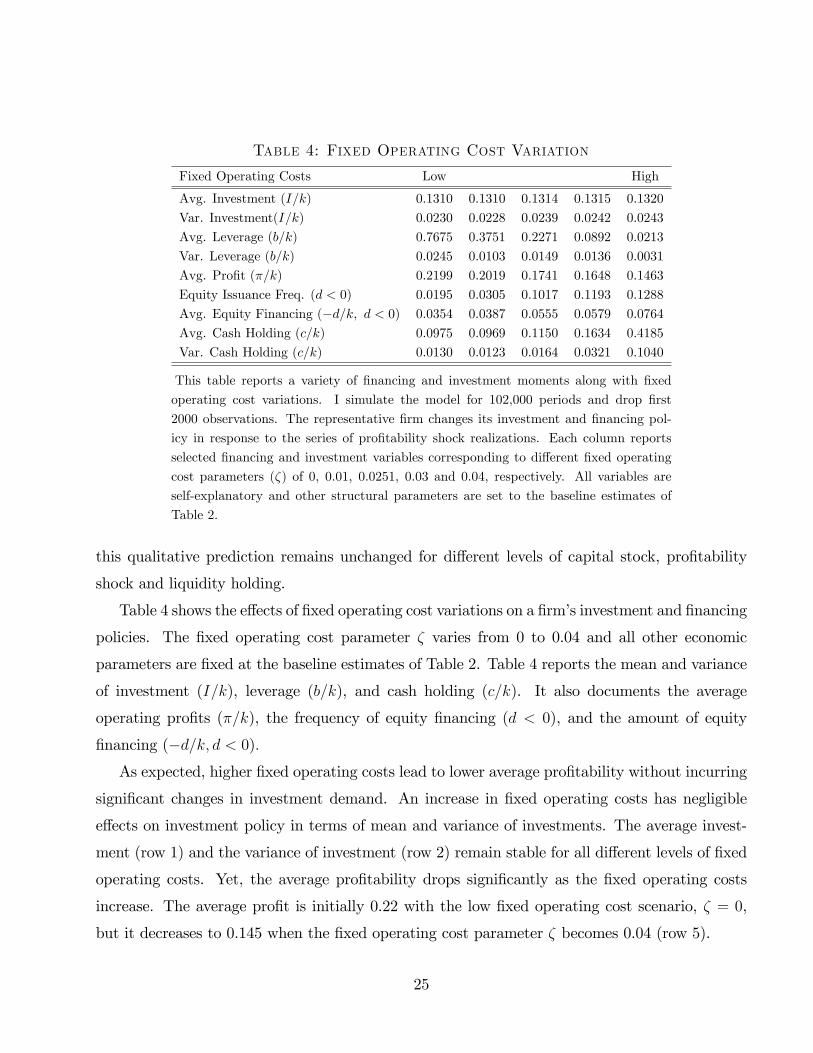
Table 4: Fixed Operating Cost Variation

Fixed Operating Costs Low High

Avg. Investment (I=k) 0.1310 0.1310 0.1314 0.1315 0.1320

Var. Investment(I=k) 0.0230 0.0228 0.0239 0.0242 0.0243

Avg. Leverage (b=k) 0.7675 0.3751 0.2271 0.0892 0.0213

Var. Leverage (b=k) 0.0245 0.0103 0.0149 0.0136 0.0031

Avg. Pro�t (�=k) 0.2199 0.2019 0.1741 0.1648 0.1463

Equity Issuance Freq. (d < 0) 0.0195 0.0305 0.1017 0.1193 0.1288

Avg. Equity Financing (�d=k; d < 0) 0.0354 0.0387 0.0555 0.0579 0.0764

Avg. Cash Holding (c=k) 0.0975 0.0969 0.1150 0.1634 0.4185

Var. Cash Holding (c=k) 0.0130 0.0123 0.0164 0.0321 0.1040

This table reports a variety of �nancing and investment moments along with �xed

operating cost variations. I simulate the model for 102,000 periods and drop �rst

2000 observations. The representative �rm changes its investment and �nancing pol-

icy in response to the series of pro�tability shock realizations. Each column reports

selected �nancing and investment variables corresponding to di¤erent �xed operating

cost parameters (�) of 0, 0.01, 0.0251, 0.03 and 0.04, respectively. All variables are

self-explanatory and other structural parameters are set to the baseline estimates of

Table 2.

this qualitative prediction remains unchanged for di¤erent levels of capital stock, pro�tability

shock and liquidity holding.

Table 4 shows the e¤ects of �xed operating cost variations on a �rm�s investment and �nancing

policies. The �xed operating cost parameter � varies from 0 to 0.04 and all other economic

parameters are �xed at the baseline estimates of Table 2. Table 4 reports the mean and variance

of investment (I=k), leverage (b=k), and cash holding (c=k). It also documents the average

operating pro�ts (�=k), the frequency of equity �nancing (d < 0), and the amount of equity

�nancing (�d=k; d < 0):As expected, higher �xed operating costs lead to lower average pro�tability without incurring

signi�cant changes in investment demand. An increase in �xed operating costs has negligible

e¤ects on investment policy in terms of mean and variance of investments. The average invest-

ment (row 1) and the variance of investment (row 2) remain stable for all di¤erent levels of �xed

operating costs. Yet, the average pro�tability drops signi�cantly as the �xed operating costs

increase. The average pro�t is initially 0.22 with the low �xed operating cost scenario, � = 0,

but it decreases to 0.145 when the �xed operating cost parameter � becomes 0.04 (row 5).

25

Table 5: Fixed Operating Cost Variation: Robustness

Variables Serial Corr.(�) Uncertainty(�) DRS(�)

Low High Low High Low High

Panel A: Low Cost (�=0.0)

Avg. Leverage(b=k) 0.8670 0.3672 0.9326 0.3708 0.9007 0.3982

Equity Freq. (d < 0) 0.0302 0.0354 0.0393 0.0091 0.0111 0.0041

Avg. Equity Financing (�d=k; d < 0) 0.0309 0.0451 0.0265 0.0435 0.1365 0.0167

Panel B: Baseline (�=0.0251)

Avg. Leverage(b=k) 0.2984 0.1190 0.2731 0.0553 0.2350 0.1590

Equity Freq. (d < 0) 0.1013 0.1009 0.0810 0.0472 0.0484 0.0448

Avg. Equity Financing (�d=k; d < 0) 0.0563 0.0710 0.0549 0.0651 0.1983 0.0280

This table reports average leverage(b=k), equity �nancing frequency(d < 0) and average equity

�nancing amount (�d=k, d < 0) based on the model with a low �xed operating cost (� = 0;

Panel A) and with the baseline �xed cost (� = 0:0251; Panel B). The �rst two columns contrast

low and high serial correlation cases in the pro�tability shock, where � = 0:6 and � = 0:8,

respectively. The next two columns are for low and high uncertainty cases in the pro�tability

shock where � is 0.12 and 0.3, respectively. The last two columns are for low and high returns

to scale scenarios of the pro�t function, where � = 0:6 and � = 0:8, respectively.

Table 4 highlights that a �rm with higher �xed operating costs tends to have lower leverage

and rely more heavily on equity �nancing. To be speci�c, the average leverage decreases by

more than 95% and the variance of leverage diminishes by almost 90% as the �xed operating

cost parameter � increases from 0 to 0.04 (row 3 and 4). Given the same �xed operating cost

variation, equity �nancing frequency increases more than ten times and the amount of equity

proceeds becomes more than doubled (row 6 and 7).

The e¤ect of �xed operating costs on cash holding policy is indeterminate. The average

cash holding slightly decreases between the �rst two columns but gradually increases afterwards

(row 8). This inconclusive direction may stem from the endogeneity in the joint decisions of

liquidity and debt policies. A higher marginal value of liquidity indicates large debt servicing

costs given the same amount of debt obligations, ex-ante. Yet, a �rm with large debt servicing

costs endogenously selects a low leverage ratio, which potentially undermines the �rm�s cash

retention incentives, ex-post. The average liquidity holding ratio re�ects these counter-balancing

e¤ects from growing debt servicing costs.

Table 5 shows the robustness of the �xed operating cost predictions on the capital structure

26

choice. The �rm with low �xed operating costs (Panel A) always relies more heavily on debt

�nancing for high and low uncertainty scenarios of the pro�tability shock, for high and low serial

correlations in operating pro�ts, and for high and low decreasing returns to scale parameters. A

�rm with low �xed operating costs also uses equity �nancing less frequently than the �rm with

the baseline �xed operating costs does, in line with the results of Table 4.

These quantitative predictions are consistent with recent empirical �ndings on the relationship

between operating leverage and external �nancing policies. Kahl et al. (2012) uniquely analyze

the e¤ect of operating leverage on a �rm�s �nancing policies. They mainly show that higher

operating leverage �rms tend to maintain lower leverage and issue equity to a greater extent.

Their �ndings are in line with the quantitative predictions of Table 4 and 5.

Prior dynamic trade-o¤ models without debt �nancing costs may not successfully generate

these quantitative predictions from the �xed operating cost variations. Appendix B reports the

comparative statics results from the models of Hennessy and Whited (2005) and DDW. In their

model simulations, a high �xed operating cost �rm is not closely associated with low leverage

and frequent equity �nancing. These results support the importance of debt servicing costs in

obtaining the quantitative predictions on capital structure choice; servicing debt incurs only

minor costs in these models because a �rm can almost freely roll over its debt obligations.

4.2 Comparative Statics II: Convex Capital Adjustment Costs

Capital installation and liquidation incur organizational costs (Hamermesh and Pfann 1997).

The accumulation and resale of capital stock lead to the hiring or �ring new workers, which

may involve training, search, or severance costs. In addition, the extant workers may �nd their

routine disrupted and their tasks reassigned when a �rm purchases or sells its capital stock. This

reallocation process may lower labor productivity and increase capital adjustment costs.

Higher convex capital adjustment costs lead to slow adjustments of capital stock and large

costs of asset sales. A high capital resale cost is especially and closely associated with large debt

servicing costs. As depicted in Figure 1, a �rm increases its asset sales to service large debt

obligations and these asset sales tend to be more costly with higher capital resale costs.

Figure 7 shows the implication of convex capital adjustment cost variations on debt servicing

costs. The marginal value of liquidity is plotted for two di¤erent levels of convex capital adjust-

27

Figure 7: Marginal Value of Liquidity : Convex Capital Adjustment Costs

0 0.1 0.2 0.3 0.4 0.5 0.6 0.7 0.8 0.9 11

1.005

1.01

1.015

1.02

1.025

1.03


Leverage, b/k

θk=Baseline

θk=High

The marginal value of liquidity is plotted at the steady state level of capital stock (kss) with zero liquidity holding

(c = 0). Two di¤erent levels of convex capital adjustment cost are examined (�k = 0:1163; �k = 3� 0:1163). Allvalues are evaluated along with the leverage ratio variation with a neutral pro�tability shock (z = 1).

ment costs, the baseline, �k = 0:1163, and high cost, �k = 3 � 0:1163, scenarios. The marginalvalue of liquidity is evaluated along with the leverage ratio at the steady state of capital stock

(kss) with a neutral pro�tability shock (z = 1) and zero liquidity holding (c = 0). All other

economic parameters are set to the values of Table 2 except the �xed capital adjustment costs:

the parameter k is set to zero to isolate the e¤ect of convex capital adjustment costs.

Figure 6 points out that a �rm with high convex capital adjustment costs faces large debt

servicing costs, especially those with a considerable amount of debt obligations. The baseline

and high convex capital adjustment cost �rms confront the same marginal value of liquidity until

the leverage ratio becomes 0.3. Yet, the high convex capital adjustment cost �rm shows a greater

marginal value of liquidity than the baseline cost �rm does when the leverage ratio is larger than

0.3. This �nding is in line with the increasing tendency of asset sales to service additional debt

obligations, as illustrated in Figure 1.

Table 6 compares investment and �nancing policies for di¤erent levels of convex capital ad-

justment costs, which vary from 0.1 to 3 times of the baseline convex capital adjustment cost

28

Table 6: Convex Capital Adjustment Cost Variation

Convex Capital Adjustment Cost Low High



Avg. Leverage (b=k) 0.1952 0.1770 0.1761 0.1655 0.1419

Var. Leverage (b=k) 0.0171 0.0129 0.0084 0.0036 0.0034

Avg. Pro�t (�=k) 0.1647 0.1681 0.1701 0.1727 0.1743





This table reports a variety of �nancing and investment moments along with �xed

operating cost variation. Each column indicates a di¤erent level of convex capital

adjustment cost; the values are 0.1, 0.5, 1, 2, and 3 times of the baseline convex capital

adjustment cost in Table 2. The �xed capital adjustment cost parameter is set to 0 and

the other parameter values are from the baseline estimates of Table 2. All variables are

self explanatory.

estimate. To focus on the role of convexity in capital adjustment costs, the �xed cost parameter

k is set to zero. All other economic parameters are �xed at the baseline estimates in Table 2.

Table 6 reports the mean and variance of investment (I=k), leverage (b=k), and cash stock (c=k).

It also documents the average operating pro�ts (�=k), the frequency of equity �nancing (d < 0),

and the amount of equity proceeds (�d=k, d < 0):Table 6 shows that a �rm with high convex capital adjustment costs is closely associated with

lower leverage and more frequent equity �nancing. The average leverage ratio drops by almost

25% as convex capital adjustment costs increase. Notice that the leverage ratio is 0.19 in the

�rst column, but decreases to 0.14 in the last column (row 3). The frequency of equity �nancing

also gradually increases from 0.5% to 3% for the same convex capital adjustment costs variation

(row 6). The average equity proceeds are stable around 5% of capital stock for all levels of

convex capital adjustment costs (row 7). Even with slightly higher pro�tability (row 5), a higher

convexity in capital adjustment costs leads to lower �nancial leverage and more frequent equity

�nancing.

Interestingly, a higher convex capital adjustment cost �rm tends to hold lower cash holding

(row 8). This appears inconsistent with a large value of liquidity from a higher convex capital

29

Figure 8: Marignal Value of Liquidity: Convex Capital Adjustment Costs andProfitability Shock

0 0.2 0.4 0.6 0.8 11.01

1.02

1.03

1.04

1.05

1.06

1.07

Leverage, b/k

Panel A. Low Profitability Shock, z=0.3

0 0.2 0.4 0.6 0.8 11

1.005

1.01

1.015

1.02

1.025

Leverage, b/k

Panel B. High Profitability Shock, z=1.5

θk= Baselineθk= High

θk= Baselineθk= High

The marginal value of liquidity is plotted at the steady state level of capital stock (kss) with zero cash holding.

Panel A describes a low pro�tability shock case (z=0.3) and Panel B describes a high pro�tability shock case

(z = 1:5). Two di¤erent levels of convex capital adjustment cost are examined (�k = 0:1163, �k = 3 � 0:1163).All values are evaluated along with the leverage ratio variation.

adjustment cost in Figure 7. Two economic forces may explain such decline in average cash hold-

ing ratio. First, endogenous decisions of leverage and cash holding potentially play an important

role, as discussed in the previous section. An economic environment generating large debt ser-

vicing costs raises the marginal value of liquidity, given the same amount of debt obligations,

ex ante. However, a �rm optimally maintains lower leverage, which potentially undermines cash

holding incentives, ex post. The latter e¤ects could be more signi�cant in the convex capital

adjustment costs variation.

To investigate another potential reason for the diminishing cash holding tendency, Figure

8 examines the relationship between convex capital adjustment costs and the marginal value

of liquidity, for two di¤erent levels of the pro�tability shock. The marginal value of liquidity is

evaluated for the baseline and high convex capital adjustment costs (�k = 0:1163, �k = 3�0:1163)at the steady state level of capital stock (kss) with zero cash holding (c = 0). Panel A describes

30

Table 7: Convex Capital Adjustment Costs Variations: Robustness

Variables Serial Corr.(�) Uncertainty(�) DRS(�)

Low High Low High Low High

Panel A: Baseline

Avg. Leverage(b=k) 0.2051 0.1132 0.2037 0.0559 0.2045 0.1605

Equity Freq. (e > 0) 0.0154 0.1019 0.0077 0.0625 0.0163 0.0386

Avg. Equity Financing (e=k) 0.0579 0.0646 0.0480 0.0594 0.2354 0.0280

Panel B: High Convex Capital Adjustment Cost

Avg. Leverage(b=k) 0.1293 0.0936 0.1792 0.0165 0.1969 0.1276

Equity Freq. (e > 0) 0.0408 0.1330 0.0192 0.0705 0.0215 0.1257

Avg. Equity Financing (e=k) 0.0575 0.0674 0.0425 0.0854 0.2615 0.0306

This table reports average leverage (b=k), equity �nancing frequency (d > 0) and average equity �nancing

amount (d=k) calculated from the simulation of the baseline convex capital adjustment costs (�k = 0:1163;

Panel A) and high convex capital adjustment cost (�k = 3�0:1163); Panel B. The �rst two columns contrastlow and high serial correlation cases in the pro�tability shock, where � =0.6 and � =0.8, respectively. The

next two columns are for low and high uncertainty cases in the pro�tability shock where � is 0.12 and 0.3,

respectively. The last two columns are for low and high returns to scale scenarios of the pro�t function,

where � = 0.6 and � =0.8, respectively.

the case with a low pro�tability shock, z = 0:3, whereas Panel B depicts the case with a high

pro�tability shock, z = 1:5. All other economic conditions are identical to those explained in

Figure 7.

Panels A and B illustrate contrasting patterns of the marginal value of liquidity for the

baseline and high convex capital adjustment cost �rms, depending on the pro�tability shock

realizations. While the baseline convex capital adjustment cost �rm shows a lower marginal

value of liquidity in Panel A consistent with Figure 7, the baseline cost �rm rather exhibits a

higher marginal value of liquidity than the high convex capital adjustment cost �rm does in Panel

B. This �nding is closely associated with the role of low convex capital adjustment costs enabling

more rapid accumulation of capital stocks. Given the same high pro�tability shock realization,

the low convex capital adjustment cost �rm tries to build up a larger amount of capital stock,

which raises the marginal value liquidity more substantially. The decreasing average cash holding

ratio may stem from the higher marginal value of liquidity in a lower convex capital adjustment

cost �rm at high pro�tability shock states.

Table 7 shows the robustness of the convex capital adjustment cost predictions on the capital

31

structure choice. The external �nancing policy predictions from large debt servicing costs remain

unchanged for high and low uncertainty cases in the pro�tability shock, for high and low serial

correlations in operating pro�ts, and for high and low decreasing returns to scale parameters.

Consistent with the result in Table 6, the higher convex capital adjustment cost �rm (Panel B)

always uses equity �nancing more frequently and maintains lower leverage than the baseline cost

�rm does (Panel A).

The frequent equity �nancing and low leverage in human capital intensive �rms are closely

associated with the results of Table 6 and 7. Hall (2002) points out the rigidity in wage payments

and the �rm speci�city of human capital stocks as economic forces behind large organizational

costs of adjusting R&D expenditures. Consistent with the external �nancing regularities in R&D

intensive �rms, my model predicts that a �rm with higher convex capital adjustment costs tends

to show low leverage and use equity �nancing more actively.

The debt servicing cost predictions on convex capital adjustment costs di¤er markedly from

DDW. In their model, a �rm with high convex capital adjustment costs shows higher leverage,

which contrasts the above predictions. With limited debt capacity, a low convex capital adjust-

ment cost �rm has an additional incentive to save its debt capacity to prepare for highly volatile

investment demands. This incentive of debt capacity preservation drives lower leverage in a �rm

with low convex capital adjustment costs. Yet, the issuance of debt does not involve any explicit

costs in their model, which potentially underestimates the e¤ects of increasing asset sales cost

on a �rm�s debt policy.

5 Empirical Analysis

This section provides empirical evidence supporting the model�s quantitative predictions from

large debt servicing costs. Leverage ratio, debt conservatism measure (Graham 2000) and equity

�nancing indicators are examined as dependent variables in cross-sectional regression models.

I follow Boulin et al. (2011) in their implementation of Graham�s (2000) debt conservatism

measure. The detailed measure construction is described in Appendix C. A large value of the

debt conservatism measure indicates a more conservative debt policy.

32

5.1 Convex Capital Adjustment Costs

To analyze the implications of convex capital adjustment costs on capital structure choice, I �rst

calculate a �rm level convex adjustment cost estimate by using a modi�ed version of Tobin�s

q regression. Similar to Eberly�s (1997) approach, I regress a �rm�s investment-asset ratio on

Tobin�s q, operating pro�ts, and the investment good price for each �rm, but only when the

�rm�s investment is positive. The operating pro�t term is introduced to capture the e¤ect of

�nancing constraints, as in Fazzari, Hubbard and Petersen (1988). This inclusion is in line with

an important role of external �nancing costs in my model. To capture non-convexity in capital

expenditure, the regression is only conducted for positive investment �rm-year observations. The

regression model is summarized as follows:

I

K= �0 + �1Tobin�s q + �2pro�t+�3investment good price+ " for I > 0: (15)

After assignment of the �rm level convex capital adjustment cost estimate, I drop �rms with

negative capital adjustment costs because the quantitative predictions only hold for the positive

costs region. Each �rm is grouped by its two digit SIC code �rst, and then it is categorized

into convex capital adjustment cost quartiles within its industry group. Since the convex capital

adjustment cost is inversely related to �1, the �rms in the �rst quartile have the highest convex

capital adjustment cost estimates and the �rms in the fourth quartile have the lowest ones.

Table 8 reports summary statistics for each convex capital adjustment cost quartile category.

The table documents the average of leverage ratio, debt conservatism, cash holding, and operating

pro�ts. The frequency of equity �nancing is also reported. The table considers only the �rms with

at least 12 observations during the sample period, which provides a more reliable convex capital

adjustment cost estimate. Appendix E contains the analysis based on the �rms with at least 6

�rm-year observations. Appendix E con�rms that the qualitative predictions remain unchanged

in both summary statistics and regression models by the inclusion of younger �rms. High-tech and

non high-tech sub-categories are introduced to examine whether the overall summary statistics

results stem from high-tech industries, which are well known for low leverage and frequent equity

�nancing (Hall 2002).

Table 8 indicates more conservative debt policy and frequent equity �nancing in high convex

33

Table 8: Summary Statistics : Convex Capital Adjustment CostQuartile

Observations Equity Freq. Leverage Cash Pro�t Conservatism

Panel A: All Firms

1st Quartile 6415 0.2023 0.2015 0.1817 0.0909 2.9844

2nd Quartile 6303 0.1988 0.2113 0.1668 0.0924 2.6283

3rd Quartile 6268 0.1903 0.2399 0.1415 0.0805 2.05

4th Quartile 5307 0.1577 0.2726 0.1225 0.0873 1.5757

Panel B: Non High-tech Firms

1st Quartile 4555 0.1488 0.2349 0.1182 0.1204 3.1229

2nd Quartile 4541 0.144 0.2406 0.1059 0.1202 2.6877

3rd Quartile 4658 0.1453 0.2634 0.0951 0.1139 2.2295

4th Quartile 3900 0.1131 0.3052 0.0781 0.1152 1.6128

Panel C:High-tech Firms

1st Quartile 1860 0.3333 0.1196 0.3373 0.0186 2.6232

2nd Quartile 1762 0.34 0.1356 0.3238 0.0207 2.4677

3rd Quartile 1610 0.3205 0.1718 0.2756 -0.0159 1.5127

4th Quartile 1407 0.2814 0.1823 0.2455 0.0099 1.4689

This table reports a variety of summary statistics for all �rms, high-tech �rms and non-high-

tech �rms according to convex capital adjustment cost quartiles. Only the �rms with at least

12 �rm-year observations are included in the calculations. Firms are included in the high-

tech category if their �rst three digit SIC code is 283, 357, 366, 382, 384, and 737, and all

other �rms are all in non high-tech category. All values are averaged except the number of

observations. The variable construction is illustrated in Appendix D.

capital adjustment cost �rms. Even though each category has stable average pro�tability, high

convex capital adjustment cost �rms tend to have low leverage ratios and large debt conservatism

measures. The average leverage ratio is 0.2015 in the �rst quartile and rises to 0.2726 in the

fourth quartile. Similarly, the debt conservatism measure decreases from 2.98 to 1.58 in response

to the same quartile variation. Firms with higher convex capital adjustment costs also use

equity �nancing more frequently. The equity �nancing frequency is 20% in the �rst quartile

and decreases to 15% in the fourth quartile. The sub-categorization of high-tech and non high-

tech industry does not in�uence the qualitative predictions from convex capital adjustment costs

quartile variations.

Table 9 investigates the relationship between convex capital adjustment cost quartile dummies

and external �nancing policies in cross-sectional regression models. The leverage ratio, debt

34

Table 9: Cross-sectional Analysis : Convex Capital Adjustment CostQuartile

Leverage Conservatism Equity

M/B ratio -0.0141 -0.0116 0.5452 0.5139 0.4062 0.4092

(0.000) (0.000) (0.000) (0.000) (0.000) (0.000)

logAsset 0.0133 0.0147 0.4685 0.4530 -0.0471 -0.0551 -0.0460

(0.000) (0.000) (0.000) (0.000) (0.000) (0.000) (0.000)

Tangibility 0.1679 0.1452 -1.5290 -1.2773 0.3224 0.4326 0.3146

(0.000) (0.000) (0.000) (0.000) (0.003) (0.000) (0.005)

Pro�tability -0.2021 -0.2042 6.2191 6.2274 -3.1357 -2.8459 -3.1450

(0.000) (0.000) (0.000) (0.000) (0.000) (0.000) (0.000)

R&D expenditure -0.1814 -0.2004 0.3535 0.5980 1.5282 3.9500 1.4838

(0.000) (0.000) (0.307) (0.081) (0.000) (0.000) (0.000)

R&D dummy -0.0191 -0.0180 -0.3712 -0.3959 0.1281 0.1585 0.1368

(0.000) (0.000) (0.000) (0.000) (0.014) (0.002) (0.009)

Med. Industry Leverage 0.2066 0.2452 -3.2308 -3.6798 0.2148 -0.8196 0.2445

(0.000) (0.000) (0.000) (0.000) (0.513) (0.013) (0.461)

Convex Cost: 1st Quartile -0.0540 0.5956 0.2938 -0.0350

(0.000) (0.000) (0.000) (0.591)

Convex Cost: 2nd Quartile -0.0478 0.4833 0.3188 0.1064

(0.000) (0.000) (0.000) (0.087)

Convex Cost: 3rd Quartile -0.0286 0.1277 0.2694 0.1284

(0.000) (0.007) (0.000) (0.036)

Stock Return(3year) 0.2238 0.3685 0.2234

(0.000) (0.000) (0.000)

Constant 0.1206 0.1434 -0.3888 -0.5595 -2.5248 -2.2340 -2.5928

(0.000) (0.000) (0.000) (0.000) (0.000) (0.000) (0.000)

N 24293 24293 22301 22301 22119 22119 22119

Adjusted R2 0.1544 0.1634 0.3016 0.3071

Pseudo R2 0.1785 0.1429 0.1791

This table reports coe¢ cients, p-values (in parenthesis) and adjusted (pseudo-) R2 from cross sec-

tional regression and logit models. The leverage ratio, debt conservatism measure, and binary

choice of equity issuance (logit) are used as dependent variables. Several control variables and

convex capital adjustment cost quartile dummies are used as independent variables. The construc-

tion of controlling variables is explained in Appendix D. Only the �rms with at least 12 �rm-year

observations are included in the estimation. The standard errors of the regressions are robust to

heteroscedasticity.

35

conservatism measure, and binary decisions of equity �nancing are used as the left-hand side

variables. On the right hand side, I employ the convex capital adjustment cost quartile dummies

and a set of widely used �rm characteristics as control variables. The control variables include

the logged book asset values, asset tangibility, market to book ratio, R&D expenditure, R&D

activity and industry median leverage ratio, as suggested in Frank and Goyal (2008). I also

introduce the 3-year stock return in the equity �nancing analysis to capture the market timing

aspect of equity �nancing. I use the ordinary least squares method in the leverage and debt

conservatism measure analysis and adopt a logit model for the binary choice of equity issuance

decisions.

As expected, �rms with higher convex capital adjustment costs exercise more conservative

debt policy. Even after controlling for the �rm characteristics, the quartile dummies show a

monotonic relation with the leverage ratio and debt conservatism measure. A higher convex

capital adjustment cost dummy variable is more negatively correlated with the leverage ratio

and positively correlated with the debt conservatism measure.

The logit regression results partially support more frequent equity �nancing in large convex

capital adjustment cost �rms. Without inclusion of the market to book ratio, higher convex

capital adjustment cost dummies are positively and almost monotonically correlated with equity

issuance decisions. Yet, the inclusion of the market to book ratio drastically changes the coef-

�cients of quartile dummies, especially for the �rms with the largest convex capital adjustment

cost estimates.

The drastic changes of quartile coe¢ cients in the logit model are probably related to the

information of the market to book ratio captured in the convex capital adjustment cost dummies.

In the estimation of �rm level convex capital adjustment costs, I use a �rm�s Tobin�s q value

as an independent variable, which is a modi�cation of the market to book ratio. The market

to book variation may directly re�ect more signi�cant information regarding equity �nancing

decisions.

To summarize, �rms with higher convex capital adjustment costs tend to use debt more

conservatively and equity �nancing more frequently, even after considering industry and other

�rm characteristics. Both of the summary statistics and regression analysis results generally

con�rm these tendencies. These �ndings are consistent with the debt servicing cost predictions

from the model simulations.

36

5.2 Future Investments and Capital Structure Choice

This section analyzes how future investment demands in�uence current external �nancing poli-

cies. Large future investments increase the marginal value of liquidity, after controlling for a

�rm�s operating pro�ts. By similar reasoning, small future investment demands are closely as-

sociated with low debt servicing costs.

To analyze the in�uence of future investments on capital structure choices, I construct indi-

cator variables based on actual future capital expenditure. The use of indicator variables helps

relieve a potential measurement error problem stemming from the use of actual future invest-

ments as explanatory variables. Unexpectedly great or poor investment opportunities in the next

period a¤ect actual future investments and the use of indicator variables partially �lters out such

unexpected components by covering a wide range of actual investments.

To construct dummy variables indicating large and small future investments, I �rst calculate

the ranking of the investment-asset ratio for each �rm-year observation relative to all of the

�rm�investment-asset ratios in the sample periods. Then I categorize each �rm-year observation

into a quartile corresponding to its investment-asset ratio ranking. The indicator variable for

large future investment takes one if a �rm�s next period investment-asset ratio is in the fourth

quartile, and zero otherwise. Similarly, the small investment dummy takes one if a �rm�s next

period investment-asset ratio is in the �rst quartile, and zero otherwise

Table 10 documents summary statistics results according to the future investment indicator

variables. The table reports the average of leverage ratio, debt conservatism, cash holding, and

operating pro�ts. The equity �nancing frequency is also documented. The summary statistics

are calculated for di¤erent sub-categories such as high-tech industry, non high-tech industries,

young �rms and old �rms. I introduce the high-tech category to capture the in�uence of human

capital intensive �rms, well known for low leverage and frequent equity �nancing (Hall 2002).

The young-old �rm categories are also examined because younger �rms tend to maintain lower

leverage and use equity �nancing more frequently (Frank and Goyal 2003).

Consistent with debt servicing cost predictions, �rms with large future investments are closely

associated with low leverage, more conservative debt policy and frequent equity �nancing despite

higher pro�tability levels. Conversely, �rms with small future investments are correlated with

higher leverage, less conservative debt policy and infrequent equity �nancing, in spite of lower

37

Table 10: Summary Statistics : Future Investments

Equity Leverage Cash Pro�t Conservatism

Panel A : All Firms

Small Future Investments 0.1995 0.2555 0.174 0.0257 1.8741

Others 0.2404 0.2379 0.1705 0.0416 2.1588

Large Future Investments . 0.2942 0.188 0.197 0.0905 2.8486

Panel B: Old Firm-Year Observation


Others 0.1196 0.2358 0.1286 0.0979 2.5487


Panel C: Young Firm-Year Observation

Small Future Investments 0.2843 0.2524 0.2118 -0.0233 1.3488

Others 0.3372 0.2395 0.2041 -0.0036 1.7167


Panel D: Non High-tech Firms


Others 0.1859 0.2735 0.1094 0.084 2.2437


Panel E: High-tech Firms

Small Future Investments 0.3194 0.1556 0.3336 -0.0731 1.7712

Others 0.3692 0.1539 0.3149 -0.0588 1.9492


This table reports a variety of summary statistics for all �rms, young-�rm year old-�rm year,

high-tech �rms and non-high-tech �rms according to future investment dummies. Young �rm-year

observation indicates all �rms that stay less than 12 years in CRSP/Compustat database or the

�rst 12 �rm-year observations for the �rms that stay more than 12 years in the database. The other

descriptions are identical to those of Table 8

pro�tability levels. For instance, the average leverage ratio is 0.255 for �rms with small future

investments but 0.188 for �rms with large future investments. Equity �nancing frequency is 29.5%

for the �rms with large future investments but 20% for the �rms with large future investments.

The qualitative predictions remain unchanged for the sub-categories of high-tech, non-high-tech,

young �rms and old �rms.

Table 11 investigates the relationship between future investments and current capital struc-

ture choice in cross-sectional regression models. All regression and logit model speci�cations are

identical to those of Table 9, except the inclusion of the future investments indicator variables

replacing the convex capital adjustment cost dummies. The book asset value in logs, tangibility,

market to book ratio, R&D expenditure, R&D activity and industry median leverage ratio are

38

Table 11: Cross-sectional Analysis : Future Investments


M/B ratio -0.0123 -0.0109 0.5165 0.5021 0.3817 0.3787

(0.000) (0.000) (0.000) (0.000) (0.000) (0.000)

logAsset 0.0132 0.0128 0.4471 0.4531 -0.0957 -0.0929

(0.000) (0.000) (0.000) (0.000) (0.000) (0.000)

Tangibility 0.1962 0.1960 -1.5715 -1.5768 0.3105 0.3019

(0.000) (0.000) (0.000) (0.000) (0.000) (0.000)

Pro�tability -0.1705 -0.1590 4.8101 4.6862 -2.7986 -2.8409

(0.000) (0.000) (0.000) (0.000) (0.000) (0.000)

R&D expenditure -0.2235 -0.2187 0.3566 0.3005 1.1381 1.1148

(0.000) (0.000) (0.042) (0.085) (0.000) (0.000)

R&D dummy -0.0357 -0.0359 -0.3048 -0.3045 0.0719 0.0729

(0.000) (0.000) (0.000) (0.000) (0.041) (0.038)

Med. Industry Leverage 0.1909 0.1971 -3.1396 -3.2056 0.3318 0.3110

(0.000) (0.000) (0.000) (0.000) (0.121) (0.146)

Small Future Investments 0.0112 -0.2198 -0.1536

(0.000) (0.000) (0.000)

Large Future Investments -0.0372 0.2920 0.1026

(0.000) (0.000) (0.005)

Stock Return (3year) 0.2204 0.2124

(0.000) (0.000)

Constant 0.1305 0.1322 -0.1542 -0.1265 -2.1701 -2.1362

(0.000) (0.000) (0.001) (0.005) (0.000) (0.000)

N 58143 58143 47481 47481 46914 46914

Adjusted R2 0.1653 0.1708 0.2972 0.3000

Pseudo R2 0.1906 0.1915

This table reports coe¢ cients, p-values (in parenthesis) and adjusted (pseudo-) R2 from

cross sectional regression and logit models. The leverage ratio, debt conservatism mea-

sure, and binary choice of equity issuance (logit) are used as dependent variables. Several

control variables and the indicator variables for future investment demands are used as

independent variables. The construction of controlling variables is explained in Appendix

D. The standard errors of the regressions are robust to heteroscedasticity.

39

still used as control variables. The 3-year stock returns are additionally incorporated in the logit

model for equity �nancing to capture market timing aspects.

The cross-sectional results are consistent with the debt servicing cost predictions from the

model simulations. The �rms with large future investments are closely associated with low lever-

age, conservative debt policy and frequent equity �nancing, even after controlling for other �rm

characteristics. The small future investments dummy is negatively related with the leverage ra-

tio, and positively related with the debt conservatism measure and equity �nancing, as expected.

All coe¢ cients are highly signi�cant and the signs of these coe¢ cients are in line with the debt

servicing cost predictions.

The coe¢ cients of investment dummies in equity �nancing regression contradict the pre-

dictions of the standard trade-o¤ models. The standard trade-o¤ theory predicts less frequent

equity �nancing for �rms with conservative debt policy and high pro�tability. Yet, the �rms

with large future investments use equity �nancing more frequently in spite of their conservative

use of debt and large operating pro�ts. The �rms with small investments are reluctant to issue

equity despite low pro�tability and large debt obligations, which also argues against the standard

trade-o¤ theory predictions.

The regression analysis for the leverage ratio provides an interesting result to the puzzling

negative correlation between leverage ratio and pro�tability (Frank and Goyal 2008). The in-

troduction of investment dummy variables slightly weakens the negative correlation between

pro�tability and leverage (�0:1705 ! �0:1590) and the change is statistically signi�cantly at95% level.1 The debt conservatism analysis shows a similar change of the pro�tability coe¢ cient,

which suggests the weaker correlation is not a mere coincidence. Debt servicing costs consid-

erations appear to have some explanatory power in resolving the puzzling negative correlation

between pro�tability and leverage ratio.

In summary, the relationship between future investments and current capital choices is con-

sistent with debt servicing cost predictions. Large future investments are closely associated with

currently lower leverage and more frequent equity issuance. Equity �nancing behaviors in both

small and large future investment �rms contradict the standard trade o¤ theory predictions.

The inclusion of investment variables weakens the negative correlation between pro�tability and

leverage ratio.

1The p-value is not reported here.

40

6 Conclusion

I have examined the interdependence between liquidity policy and capital structure choice and

shown it to be a key missing link in the existing literature. Debt servicing costs lie at the core

of the analysis; servicing debt is costly because it drains a �rm�s valuable liquidity. To examine

the implications of debt servicing costs on a �rm�s external �nancing policies, I developed a new

dynamic trade-o¤model with liquidity management and adopted the marginal value of liquidity

as a natural measure of debt servicing costs.

My model analysis and following empirical study yielded a number of interesting results.

First, a �rm with large debt obligations faces a higher cost of debt, even in the absence of

�nancial distress costs. Second, a smaller �rm may have lower leverage ratio because its large

investment demands increase debt servicing costs. Third, equity �nancing could be used for

cash retention, especially for �rms with large current and future investments, because it does

not deplete valuable future liquidity. Finally, my comparative statics and empirical analysis

show that large debt servicing costs are closely associated with low leverage and frequent equity

�nancing, by investigating the roles of convex capital adjustment costs, �xed operating costs,

and future investment demands on capital structure choice.

These �ndings provide novel insights on a variety of puzzling empirical regularities. Most of

all, the debt servicing costs provide an economic explanation for why a �rm may exercise conser-

vative debt policy even in the face of low �nancial costs (Graham 2000). Indeed, many economic

factors closely associated with conservative debt policy suggest the potential importance of debt

servicing costs in resolving the debt conservatism puzzle. Next, the marginal value of liquidity

directly connects large investments with lower leverage in smaller �rms (Frank and Goyal 2008),

regardless of limited debt capacity considerations (DDW). In fact, equity proceeds are primarily

used for cash retention (DeAngelo et al. 2010) and equity �nancing is generally concurrent with

large current and future investments (Loughran and Ritter 1997). This cash retention role of eq-

uity proceeds di¤ers markedly from prior theories highlighting large informational costs in equity

issuance (Myers and Majluf 1984) or the role of equity proceeds for debt payments (Strebulaev

2007).

My study highlights several lucrative opportunities for future research. Most of all, the risk

premium involved in a �rm�s debt issuance is an important topic. A large risk premium drains a

41

�rm�s liquidity more substantially, but increases the amount of interest tax shields. The trade-o¤

between large debt servicing costs and growing tax shields provides more precise understanding

on a �rm�s capital structure choice. Incorporating market timing aspect of equity �nancing is

another direction. The market timing consideration of equity �nancing is empirically important

(Baker and Wurgler 2002), but is not well captured in my model. Furthermore, future empirical

studies potentially employ more delicate methods for testing the debt servicing costs predictions

to overcome endogeneity issues in my cross-sectional models.

42

References

Altinkihc, O. and R. S. Hansen (2000). Are there economies of scale in underwriting fees?

evidence of rising external �nancing costs. The Review of Financial Studies 13 (1), 191�

218.

Blouin, J., J. E. Core, and W. Guay (2010). Have the tax bene�ts of debt been overestimated?

Journal of Financial Economics 98 (2), 195�213.

Bolton, P., H. Chen, and N. Wang (2011). A uni�ed theory of Tobin�s q, corporate investment,

�nancing, and risk management. The Journal of Finance 66 (5), 1545�1578.

Bolton, P., H. Chen, and N. Wang (2013). Market timing, investment, and risk management.

Journal of Financial Economics 109 (1), 40�62.

Brown, J. R., S. M. Fazzari, and B. C. Petersen (2009). Financing innovation and growth:

Cash �ow, external equity, and the 1990s R&D boom. The Journal of Finance 64 (1),

151�185.

Cooper, R. W. and J. C. Haltiwanger (2006). On the nature of capital adjustment costs. The

Review of Economic Studies 73 (3), 611�633.

David McLean, R. (2011). Share issuance and cash savings. Journal of Financial Eco-

nomics 99 (3), 693�715.

DeAngelo, H., L. DeAngelo, and R. M. Stulz (2010). Seasoned equity o¤erings, market timing,

and the corporate lifecycle. Journal of Financial Economics 95 (3), 275�295.

DeAngelo, H., L. DeAngelo, and T. M. Whited (2011). Capital structure dynamics and tran-

sitory debt. Journal of Financial Economics 99 (2), 235�261.

Denis, D. J. and S. B. McKeon (2012). Debt �nancing and �nancial �exibility evidence from

proactive leverage increases. Review of Financial Studies 25 (6), 1897�1929.

Eberly, J. C. (1997). International evidence on investment and fundamentals. European Eco-

nomic Review 41 (6), 1055�1078.

Fama, E. F. and K. R. French (2002). Testing trade-o¤ and pecking order predictions about

dividends and debt. The Review of Financial Studies 15 (1), 1�33.

43

Fama, E. F. and K. R. French (2005). Financing decisions: Who issues stock? Journal of

Financial Economics 76 (3), 549�582.

Fischer, E. O., R. Heinkel, and J. Zechner (1989). Dynamic capital structure choice: Theory

and tests. The Journal of Finance 44 (1), 19�40.

Frank, M. Z. and V. K. Goyal (2009). Capital structure decisions: Which factors are reliably

important? Financial Management 38 (1), 1�37.

Gamba, A. and A. Triantis (2008). The value of �nancial �exibility. The Journal of Fi-

nance 63 (5), 2263�2296.

Graham, J. R. (2000). How big are the tax bene�ts of debt? The Journal of Finance 55 (5),

1901�1941.

Hall, B. H. (1987). The relationship between �rm size and �rm growth in the us manufacturing

sector. The Journal of Industrial Economics 35 (4), 583�606.

Hall, B. H. (2002). The �nancing of research and development. Oxford review of economic

policy 18 (1), 35�51.

Hennessy, C. A. and T. M. Whited (2005). Debt dynamics. The Journal of Finance 60 (3),

1129�1165.

Hennessy, C. A. and T. M. Whited (2007). How costly is external �nancing? Evidence from a

structural estimation. The Journal of Finance 62 (4), 1705�1745.

Kahl, M., J. Lunn, and M. Nilsson (2012). Operating leverage and corporate �nancial policies.

AFA 2012 Chicago Meetings Paper .

Leary, M. T. and M. R. Roberts (2005). Do �rms rebalance their capital structures? The

Journal of Finance 60 (6), 2575�2619.

Loughran, T. I. M. and J. R. Ritter (1997). The operating performance of �rms conducting

seasoned equity o¤erings. The Journal of Finance 52 (5), 1823�1850.

Modigliani, F. and M. H. Miller (1958). The cost of capital, corporation �nance and the theory

of investment. The American economic review 48 (3), 261�297.

Myers, S. C. and N. S. Majluf (1984). Corporate �nancing and investment decisions when

�rms have information that investors do not have. Journal of Financial Economics 13 (2),

44

187�221.

Riddick, L. A. and T. M. Whited (2009). The corporate propensity to save. The Journal of

Finance 64 (4), 1729�1766.

Shyam-Sunder, L. and S. C. Myers (1999). Testing static tradeo¤against pecking order models

of capital structure. Journal of Financial Economics 51 (2), 219�244.

Strebulaev, I. A. (2007). Do tests of capital structure theory mean what they say? The Journal

of Finance 62 (4), 1747�1787.

Whited, T. M. (1992). Debt, liquidity constraints, and corporate investment: Evidence from

panel data. The Journal of Finance 47 (4), 1425�1460.

45

Appendix

A Simulated Method of Moments

The table A.1 report the de�nition of real and �nancial variables from the CRSP/Compustat

database. The symbols in parenthesis refer to the items in CRSP/Compustat merged database.

Table A.1: Definition of Variables used in the SMM estimation

Variable De�nition

Investment (Capital Expenditures (CAPX) � Sale of Property, Plant and Equipment

(SPPE) +Acquisitions (AQC))/Property, Plant and Equipment � Total

(GROSS, PPEGT)

Leverage Long-Term Debt � Total (DLTT)/ (Assets - Total (AT) � Cash and Short-

Term Investments (CHE))

Cash Cash and Short �Term Investments (CHE) / (Assets - Total (AT) � Cash and

Short-Term Investments (CHE))

Dividends(Equity) (Cash Dividends (DV) + Purchase of Common and Preferred Stock(PRSTKC)

� Sale of Common and Preferred Stock (SSTK)) / (Assets - Total (AT)� Cash

and Short-Term Investments (CHE))

Tobin�s Q (End of year price (PRCC_F) � Number of Common Shares Outstanding

(CSHO) + Long-Term Debt - Total (DLTT) � Cash and Short-Term Invest-

ments (CHE)) /Property, Plant and Equipment - Total (GROSS, PPEGT)

Operating Pro�t Earnings Before Interest, Taxes, Depreciation and Amortization (EBITDA) /

(Assets - Total (AT) � Cash and Short-Term Investments (CHE))

Global identi�cation of a simulated moments estimator is achieved if the expected value of

the di¤erence between the simulated moments and the data moments equals zero if and only

if the structural parameters equal their true values. To �nd the minimizing parameter values,

I employ the simulate annealing method, a global optimization procedure based on parameter

simulations.

To correctly identify structural parameters, I pick up the following 13 moments. The iden-

ti�cation scheme is similar to the strategy of DDW. Average and variance of investment help

to identify the adjustment cost parameters� k; �k

�. A higher convex capital adjustment cost

decreases the average and variance of investment and a higher �xed capital adjustment cost raises

the variance of investment. Average operating pro�ts helps to identity the curvature of pro�t

46

function (a) and the �xed operating costs (�): As discussed in DDW, a higher � raises average

pro�t (zk� � �kss=k) and a higher operating leverage (�) lowers average operating pro�ts. The

serial correlation of the pro�tability shock (�) and the �xed operating parameter (�) a¤ects the

serial correlations in operating pro�ts. A higher �xed operating cost increases the correlations

in pro�t generation. The variance of pro�t helps to capture the uncertainty parameter of pro�t

evolution (�). The average dividends and Tobin�s q are closely associated with a �rm valuation.

The other moment selections pertain to a �rm�s �nancing decision. The frequency of equity

�nancing and average amount of equity �nancing play important roles in the identi�cation of

�xed ( e) and convex equity issuance cost (�e) : The average leverage ratio and the variance of

leverage helps to pin down the baseline debt �nancing cost� b�and the additional �nancing

cost component��b�: A higher baseline �nancing cost lowers the average leverage. A higher ad-

ditional �nancing cost decreases the variance of leverage because it provides additional incentive

to maintain debt obligations from the option value of debt issuance. The mean and variance of

cash holding ratio also help to identify these two debt �nancing costs. A high debt �nancing

costs� b�provides additional incentive to cash retention because it exacerbates a �rm�s �nancial

frictions. The additional component governs the option value of debt issuance and a higher cost��b�implies large incentives to save cash.

The SMM objective function is a weighted sum of squared errors, in which the "errors" are

given by the di¤erence between the empirical moments vector and its model counterpart. The

vector of empirical moments asM(x), in which x is an i. i.d data sample. The vector of simulated

moments is denoted as m(y; �), in which y is a simulated data sample. I denote the objective

function as Q(x; y; �):

Q(x; y; �) = (M(x)�m(y; �))0W (M(x)�m(y; �))

If I denote J be the ratio of the number of observations in the simulated data set to the

number observations in the real data set (N). By choosing the optimal weighting matrix W, the

covariance matrix ofpN��̂ � �

�can be written as follows:

pN��̂ � �

�~

�1 +

1

J

��@

@�m(y; �)0W

@

@�m(y; �)

��1:

47

The test of the over-identifying restrictions can be denoted as:

NJ

1 + JQ(x; y; �):

To achieve a numerical solution of model, I use the value function iteration method, which

requires to discretize state spaces for the four state variables. The state variable constructions

are very similar to Hennessy and Whited (2005, 2007), and DDW. The space of capital stock lies

on the following points:

[�k(1� �)20; :::; �k(1� �)1=2; �k]:

The boundness of �k for a decreasing returns to scale pro�t function �; is discussed in Hennessy

and Whited (2005).

The productivity shock (z) is modelled to have 12 points. I transform AR(1) process into a

discrete state Markov chain on the interval of [�4�; 4�]. Tauchen (1986) argues that 8~9 pointsare enough to approximate the AR(1) process. The upper bound for debt balance

��b�is obtained

if I assume the upper bound for cash balance(�c) is a half of the upper bound of debt balance�12(�b)�; the same as in DDW. I let the debt (b) state have equally spaced 25 points in the interval

of [0;�b] and the cash (b) state have equally spaced 12 points in the interval of [0; �c]:2

B Simulations of Prior Models

This section contains simulation results of prior models for di¤erent levels of �xed operating

costs and convex capital adjustment costs. In Table B.1. and B.2, the �rst panel is based on the

baseline model with very low debt �nancing costs analogous to DDW. The baseline �nancing

cost is set to 0 and the additional debt �nancing cost component is set to 0.0002. The second

panel is based on the baseline model with a �re sale discount similar to Hennessy and Whited

(2005). If a �rm�s next period debt payment (b0(1 + r)) is larger than the sum of next period

after tax pro�t (�0 � Tax), liquidity (c0(1 + r)) and capital stock after depreciation (k(1� �)),

then the �rm has to liquidate its capital stock with the resale price of s: I set the resale discount

s = 0:75 the same value used in the simulation of Hennessy and Whited (2005). The baseline

2DDW has net debt space with 29 points covering both cash and debt balance.

48

and additional �nancing cost set to 0 and 0.0002 respectively.

In the �xed operating cost analysis of Table B.1 , the model of DDW matches the leverage

variation but is unsuccessful in generating equity issuance predictions. Hennessy and Whited

(2005) with �re sale discount generates non-monotonic change in leverage contradictory to debt

servicing cost predictions.

In the convex capital adjustment cost analysis of Table B.2 , both of the models show

monotonically increasing leverage patterns, contrary to the baseline model predictions. This

direction in leverage variation is consistent with the limited debt capacity consideration of DDW.

49

Table B.1: Summary Statistics for Distinctive Operating andFixed Equity Financing Costs

Fixed Operating Costs Low High

Panel A: DDW



Avg. Leverage (b=k) 1.0544 1.0096 0.4971 0.2970 0.2128

Var. Leverage (b=k) 0.0376 0.0494 0.0248 0.0265 0.0259

Avg. Pro�t (�=k) 0.2182 0.2013 0.1723 0.1641 0.1480





Panel B : Hennessy and Whited (2005)



Avg. Leverage (b=k) 0.4084 0.4326 0.3541 0.2830 0.0967

Var. Leverage (b=k) 0.0368 0.0356 0.0223 0.0182 0.0112

Avg. Pro�t (�=k) 0.2197 0.2016 0.1742 0.1650 0.1465





This table reports a variety of moment statistics along with �xed operating cost vari-

ation. Panel A simulates the model of DDW and Panel B simulates the model of

Hennessy and Whited (2005), as described in Appendix B. Each column reports se-

lected �nancing and investment variables corresponding to di¤erent �xed operating

cost parameters (�) of 0, 0.01, 0.0251, 0.030 and 0.04, respectively. All variables are

self-explanatory and other structural parameters are set to the baseline estimates.

50

Table B.2: Summary Statistics for Distinctive Operating andFixed Equity Financing Costs

Convex Capital Adjustment Costs Low High

Panel A: DDW



Avg. Leverage (b=k) 0.3449 0.4025 0.4079 0.4062 0.4197

Var. Leverage (b=k) 0.0376 0.0201 0.0193 0.0177 0.0190

Avg. Pro�t (�=k) 0.1646 0.1678 0.1697 0.1724 0.1742





Panel B : Hennessy and Whited (2005)



Avg. Leverage (b=k) 0.1584 0.2597 0.3073 0.3737 0.3749

Var. Leverage (b=k) 0.0199 0.0191 0.0212 0.0212 0.0197

Avg. Pro�t (�=k) 0.1654 0.1681 0.1701 0.1725 0.1743





This table reports a variety of moment statistics from the baseline model simulations.

Panel A simulates the model of DDW and Panel B simulates the model of Hennessy

and Whited (2005), as described in Appendix B. Each column indicates a di¤erent

level of convex capital adjustment cost; the values are 0.1, 0.5, 1, 2, and 3 times of

the baseline convex capital adjustment cost of Table 2, respectively. The �xed capital

adjustment cost parameter is set to 0 and the other parameter values are from the

baseline estimation. All variables are self explanatory.

51

C Debt Conservatism Measure Simulation

I follow Bloulin, Core and Guay (2011)�s approach to construct Graham�s debt conservatism

measure. I de�ne a �kink� as the �rst interest payment increment at which the �rm has a

decline in its marginal tax rate (at least 50 basis points). The marginal tax rates (MTR) are

estimated by deducting various increments of the current interest payments from the taxable

income, and the kink is the increment of interest expense immediately before which results in

the computed MTR dropping by at least 50 basis points. I follow the interest deduction schedule

of Graham (2000); I add the following increments of current interest payments to before-�nancing

taxable income: 0%; 20%; 40%; 60%; 80%; 100%; 120%; 160%; 200%; 300%; 400%; 500%; 600%;

700%; and 800%. The before taxable income is de�ned as follows:

EBIT+Special Items(SPI)

- Deferred Tax Expense (TXDC) /maximum statutory tax rate

+Extraordinary Items and Discontinued Operations (XIDO)/(1-maximum statutory tax rate),

where the symbols in parenthesis refer to the items in CRSP/Compustat merged database.

I simulate future interest expenses based on the changes in the interest coverage ratio. So long

as income at t is positive, future interest is changed by the ratio of income at t to income at t-1.

If income at t is negative, I hold interest expenses constant for that year (i.e., interest expenses

at time t = interest expenses at time t-1). In terms of past interest deductions, the interest

expenses in historical taxable income is retroactively adjusted. For example, when estimating

the MTR at the 50% interest deduction increment at time t, I assume that interest deductions

in periods t-n to t-1 are set to 50% of actual.

I do not incorporate the state tax rate and alternative minimum tax rate by following the

approach of Bloulin et al. (2011). They mainly pointed out the consistency problem in the

application of alternative minium tax rate. I re�ect the historical carry backward and forward

changes into our simulation as well.

52

D Data Construction: Empirical Analysis

I introduce several control variables for emprical analyses on capital structure choices, as proposed

in Frank and Goyal (2008). Some variables are rede�ned by following prior literature.

Table D.1: Definition of Variables used in the Empirical Analyses

Variable De�nition

Asset (De�ated) Assets - Total (AT)

Pro�tability Earnings Before Interest (EBITDA) / Assets - Total (AT)

Tangibility Property, Plant and Equipment - Total (Net, PPENT)/ Assets - Total (AT)

R&D expenditure Research and Development Expense (XRD)/ Assets - Total (AT)

Market to Book (End of year price (PRCC_F)�Number of Common Shares Outstanding

(CSHO) + Long-Term Debt - Total (DLTT))/Assets - Total (AT)

Investment (Capital Expenditures (CAPX)-Sale of Property, Plant and Equipment (SPPE)

+ Research and Development Expense (XRD)/)/ Assets - Total (AT)

Tobin�s Q (End of year price (PRCC_F)�Number of Common Shares Outstanding

(CSHO)+ Long-Term Debt - Total (DLTT)�Cash and Short-Term Investments

(CHE)) /Assets - Total (AT)

Leverage Long-Term Debt - Total (DLTT)/ Assets - Total (AT)

Cash Cash and Short-Term Investments (CHE) /Assets - Total (AT)

Equity Financing (Cash Dividends (DV) + Purchase of Common and Preferred Stock(PRSTKC)

� Sale of Common and Preferred Stock (SSTK)) / (Assets - Total (AT))

E Convex Capital Adjustment Cost Regression (�6year)

This section provides the cross-sectional model results of convex capital adjustment costs for the

�rms that stay the CRSP/Compustat database at least six years. The summary statistics and

the regression results show similar patterns observed in the baseline models. Table E.1 reports

the summary statistics and Table E.2 documents the cross-sectional model results.

53

Table E.1: Summary Statistics : Convex Capital AdjustmentCost Quartile

Observations Equity Leverage Cash Cash Flow Conservatism

Panel A: All Firms

1st Quartile 8392 0.2380 0.2045 0.1997 0.0597 2.7815

2nd Quartile 8383 0.2215 0.2175 0.167 0.0686 2.3938

3rd Quartile 8055 0.2303 0.2497 0.1565 0.0557 1.8456

4th Quartile 5979 0.2000 0.2948 0.1337 0.0544 1.2343

Panel B: Non high-tech Firms

1st Quartile 5802 0.1806 0.2431 0.1286 0.0988 2.8949

2nd Quartile 5992 0.1659 0.248 0.1049 0.107 2.5057

3rd Quartile 5866 0.1742 0.2816 0.1022 0.0997 1.9939

4th Quartile 4378 0.1546 0.3271 0.0852 0.0883 1.2581

Panel C: high-tech Firms

1st Quartile 2590 0.3664 0.118 0.359 -0.0279 2.5118

2nd Quartile 2391 0.3609 0.1411 0.3226 -0.0278 2.0963

3rd Quartile 2189 0.3805 0.1643 0.302 -0.0623 1.4331

4th Quartile 1601 0.3242 0.2064 0.2665 -0.0381 1.1672

This table reports a variety of summary statistics for all �rms, high-tech �rms and non-

high-tech �rms according to convex capital adjustment cost quartiles. Only the �rms with

at least 6 �rm-year observations are included in the calculations. Firms are included in the

high-tech category if their �rst three digit SIC code is 283, 357, 366, 382, 384, and 737, and

all other �rms are all in non high-tech category. All values are averaged except the number

of observations.

54

Table E.2: Cross-sectional Analysis : Convex Capital AdjustmentCost Quartile


M/B ratio -0.0141 -0.0116 0.5452 0.5139 0.4062 0.4092

(0.000) (0.000) (0.000) (0.000) (0.000) (0.000)

logAsset 0.0133 0.0147 0.4685 0.4530 -0.0471 -0.0551 -0.0460

(0.000) (0.000) (0.000) (0.000) (0.000) (0.000) (0.000)

Tangibility 0.1679 0.1452 -1.5290 -1.2773 0.3224 0.4326 0.3146

(0.000) (0.000) (0.000) (0.000) (0.003) (0.000) (0.005)

Pro�tability -0.2021 -0.2042 6.2191 6.2274 -3.1357 -2.8459 -3.1450

(0.000) (0.000) (0.000) (0.000) (0.000) (0.000) (0.000)

R&D expenditure -0.1814 -0.2004 0.3535 0.5980 1.5282 3.9500 1.4838

(0.000) (0.000) (0.307) (0.081) (0.000) (0.000) (0.000)

R&D dummy -0.0191 -0.0180 -0.3712 -0.3959 0.1281 0.1585 0.1368

(0.000) (0.000) (0.000) (0.000) (0.014) (0.002) (0.009)

Med. Industry Leverage 0.2066 0.2452 -3.2308 -3.6798 0.2148 -0.8196 0.2445

(0.000) (0.000) (0.000) (0.000) (0.513) (0.013) (0.461)

Convex Cost: 1st Quartile -0.0540 0.5956 0.2938 -0.0350

(0.000) (0.000) (0.000) (0.591)

Convex Cost: 2nd Quartile -0.0478 0.4833 0.3188 0.1064

(0.000) (0.000) (0.000) (0.087)

Convex Cost: 3rd Quartile -0.0286 0.1277 0.2694 0.1284

(0.000) (0.007) (0.000) (0.036)

Stock Return(3year) 0.2238 0.3685 0.2234

(0.000) (0.000) (0.000)

Constant 0.1206 0.1434 -0.3888 -0.5595 -2.5248 -2.2340 -2.5928

(0.000) (0.000) (0.000) (0.000) (0.000) (0.000) (0.000)

N 24293 24293 22301 22301 22119 22119 22119

Adjusted R2 0.1544 0.1634 0.3016 0.3071

Pseudo R2 0.1785 0.1429 0.1791

This table reports coe¢ cients, p-values (in parenthesis), and adjusted (pseudo-) R2 from the cross-

sectional regression and logit models. The leverage ratio, debt conservatism, and binary choice of

equity issuance (logit) are used as dependent variables. Several control variables and convex capital

adjustment cost quartile dummies are used as independent variables. Only the �rms with at least

6 �rm-year observations are included in the estimation. The standard errors of the regressions are

robust to heteroscedasticity.

55

debt servicing costs and capital structurejl3271/jmp_jeonghwanlee.pdf · debt servicing costs and...

Documents