day-to-day ionospheric variations in a period of high solar activity

Journafqf Ammsphcn~ und T~errestriai Ph_vsirs. Vol. 55. No. 2. pp. 16S171, 1993. OOZl-9169/93 $X00+ .OO Prmted in Great Britain. Pergamon Press Ltd

Day-to-day ionospheric variations in a period of high solar activity

H. RISHBETH

Department of Physics, University of Southampton, Southampton SO9 5Nf-J, U.K.

(Received inJinalform 16 June 1992 ; accepted 30 July 1992)

Abstract-In November and December 1979 the solar 10.7 cm radio flux density, sunspot number, X-ray flux and EUV flux were high and very variable. The day-to-day variations of noon FZ-layer height and E- layer electron density at three ionosonde stations (Slough, Port Stanley and Huancayo) are found to be well correlated with the day-to-day variations of solar activity. The short-term E- and F-layer variations are consistent with those derived from longer-term studies.

1. SOLAR ACTIVITY IN LATE 1979

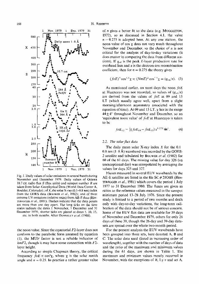
The remarkable variations of solar activity during November and December 1979 provide an excellent opportunity to study the day-to-day response of the ionosphere. The solar 10.7 cm flux density S reached the exceptional level of 374 units on 10 November 1979, with a lesser peak of 246 on 14 December and minima of 154 on 28 November and 159 on 27 December. The Ziirich sunspot number R reached maxima of 302 on 10 November and 280 on 9 December, in striking contrast to the minima of 98 on 29 November and 93 on 27 December. There can be few comparable periods in recorded history, even though the solar indices failed to match the peak values recorded two cycles previously (R = 355 on 24125 December 1957, S = 377 on 23 December 1957).

Despite the exceptional solar activity, the period was geomagnetically quiet, the daily Ap index averaging only 10 in November and 9 in December. Only two magnetic storms reached Kp = 5 ; they peaked on 13 November (Ap = 35) and 29 December 1979 (Ap = 32). The period brought the highest value of the ionospheric critical frequency ,foF2 ever recorded at Slough (U.K.), namely 17.2 MHz at 1300 and 1400 UT on 15 December 1979. With S = 239, R = 225 and Ap = 9, that day was rather ordinary as regards solar and geomagnetic activity.

DONNELLY et al. (1986) showed that, in late 1979 and early 1980, the variations of S and R were similar to those of the X-ray emissions (0.1-0.8 nm) moni-

tored by the GOES-2 satellite and the extreme ultra- violet (EUV) emissions monitored by ~nstr~ents aboard Atmospheric Explorer AE-E. These include the Fe XV, He II, H Ly 0 and H Ly a ELJV lines and UV emission at 200-205 nm. The present study is limited to the period 1 November-31 December 1979 (days 305.--365), which is almost ideal for studying day-to-day variations of solar activity with few com-

plications of seasonal changes and geomagnetic activity. Besides the satellite data and the indices S and R (Fig. l), the study uses ionosonde data from two midlatitude stations and one equatorial station (Section 2). The correlations between parameters are derived in Section 3 ; they are discussed and the best- fitting relationships presented in Section 4.

2. DATA

2.1. The ionospheric data

To study the day-to-day response of the ionosphere, ionosonde data have been taken from two mid-lati- tude stations, Slough (52N, 1W) and Port Stanley (52S, 58W) and from Huancayo (12S, 75W) near the magnetic equator. The chosen parameters were foF2, f oE, and ~(3O~)F2 (the MUF factor) at local noon, and M3000(F2) at midnight. The conventional MUF (maximum usable frequency) formula of SHIMAZAKI

(1957) was applied to estimate the height of the F2- peak :

hmF2 = 1490/(~3OOO+A~)-176[km] (1)

AM = 0.253~~(~F2~~u~) - 1.2151-0.012. (2)

AhMis the correction for ionization below the F2 layer, as given by the empirical formula (2) of DUDENEY

(1983). For the months in question, AM at noon is typically 0.15 for Port Stanley and 0.05 for Slough and the correction lowers hmF2 by 30 and 8 km, respectively, from the uncorrected values with AM = 0. At midnight, AM is negligible.

In the case of Huancayo, only noon values of foF2 are used, as the midnight F-layer data are corrupted by equatorial spread-F. Furthermore, on most days noon foE is not recorded because cf equatorial spo- radic-E (Esq). Thus, to study the day-to-day variations of E-layer ionization, the tabulated values of foE at 09 15 LT used as a estimating

165

166 H. RISHBETH

250

200 R

150

100 t

1 Nov. 1979 1 Dec. 1919 31

1 Nov. 1919 1 Dec. 1919 31

Fig. 1. Daily values of solar emissions in several bands during November and December 1979. Daily values of Ottawa 10.7 cm radio flux S (flux units) and sunspot number R are taken Gem Solar-Geophysical Data (World Data Center A, Boulder, Colorado) ; of X, the solar X-ray (0.14.8 nm) index from the GOES data (BOUWER et al., 1982); and of three extreme UV emissions (relative units) from AE-E data (HIN- TEREGGEK et al., 1981). Dashes indicate that the data points are more than one day apart. The long ticks on the time scales indicate the dates 1 November, 1 December and 31 December 1979; shorter ticks are placed at dates 5, 10, 15,

etc. in both months. After DONNELLY et al. (1986).

the noon value. Since the equatorial F2-layer does not conform to the parabolic form assumed by equation (l), the MUF factor is not a reliable indicator of hmF2, though it may have some connection with F2-

layer height. According to simple Chapman theory, the critical

frequency foE cc COS”~, where x is the solar zenith angle and n = 0.25. In practice a rather greater value

of n gives a better fit to the data (e.g. MUGGLETON,

1972), so as discussed in Section 4.1, the value n = 0.275 is adopted here. At any one station, the noon value of cos x does not vary much throughout November and December, so the choice of n is not critical for the analysis of day-to-day variations (it does matter in comparing the data from different stations). If qoE is the peak E-layer production rate for overhead Sun and c( is the electron-ion recombination coefficient, then for n = 0.275 the theory gives

(foE)4COS’.‘X cc (NmE)2 cos’ ‘x = (go&). (3)

As mentioned earlier, on most days the noon ,foE

at Huancayo was not recorded, so values of (qJcc) are derived from the values of foE at 09 and 15 LT (which usually agree well, apart from a slight morning/afternoon asymmetry associated with the equation of time). At 09 and 15 LT, x lies in the range 44k4” throughout November and December, so an ‘equivalent noon value’ of foE at Huancayo is taken to be

foE,, = ~(foE,,+,foE,,)~~*‘~W. (4)

2.2. The solar flux data

The daily mean solar X-ray index X for the O.l- 0.8 nm (l-8 A) waveband was recorded by the GOES- 2 satellite and tabulated by BOUWER et al. (1982) for 60 of the 61 days. The missing value for day 326 (an unexceptional day) was interpolated by averaging the values for days 325 and 327.

Fluxes measured in several EUV wavebands by the AE-E satellite are listed in the file SC # 210BS (HIN-

TEREGGER et al., 1981) which covers the period 1 July

1977 to 31 December 1980. The fluxes are given as ratios to the reference values measured in the sunspot

minimum period 13-28 July 1976. Since the present study is limited to a period of two months and deals only with day-to-day variations, the long-term calibration of the data should not be of serious concern. Some of the EUV flux data are available for 39 days of November and December 1979, others for only 26 days of these 39, though the 26-day and 39-day datasets are spread over the whole two-month period.

For the present analysis the EUV wavebands have been grouped into three sets, here denoted A, B and C. The solar data used (listed in increasing order of wavelength), together with the number of days of data and the ratio of the maximum and minimum values during the 61 days, are shown in Table 1. The maximum and minimum values mostly occurred in November, with the exceptions of R, Ly r and set A.

Day-to-day ionospheric variations

Table I. Solar radiations and indices used in the analysis

167

Wave band No. of days

X 61 A 26 B 39 c 26 LY fl 39 LYc* 39 R 61 s 61

Max/min ratio Wavelength band - -_-._ _ _-_____

1.29 0.1-0.8 nm 1.27 16.8G19.0, 19.0-20.4 nm 1.60 20&25.5,25.5-30.0, He II 30.4 nm 1.35 51.0-58.0, He I 58.4, 59.0-66.0 nm 1.52 102.6 nm 1.40 121.6 nm 3.25 International sunspot number 2.43 Ottawa 10.7 cm solar radio flux

The SC #ZlOBS file also contains data for five Fe lines, three of which (Fe IX, XI, XII) are within the bands of set A, the others (Fe XV 28.4 nm, Fe XVI 33.5 nm) being adjacent to set B.

3. DAY-TO-DAY CORRELATIONS

3. I ~ Correlations between solar parameters

The present work does not purport to be a con- tribution to solar physics (for which purpose the full 3.5 y data file would be available, not- just two months). Nevertheless, a limited discussion of how the solar parameters are correlated amongst themselves is needed as a background for discussing the solar- ionospheric correlations.

Accordingly, correlation coefficients have been computed for all pairings of the fluxes and indices tisted in Section 2.2, using the appropriate 39-day or Z&day subsets of larger datasets where necessary. In what follows, note that ‘correlations between bands’ (or ‘lines’) means the ‘correlation coefficients between the daily values of the tabulated fluxes’ and that in some cases the values of r for different bands or lines in a given set are averaged. Note also that the minimum values of the correlation coefficient r required for a significance level of 99%, according to the standard t-test (MORONEY, 1965, pp. 230 and 311) are as follows : for 61 pairs of data, Y = 0.32 ; for 39 pairs of data, r = 0.41 ; for 26 pairs of data, Y = 0.50. For a significance level of 99.9%, the required values are about 0.1 greater in each case, e.g. Y = 0.42 for 61 pairs of data. Fior any of the data used in this paper, therefore, values of r > 0.5 may be regarded as very significant. The main conclusions are :

1. Within any one of the sets A, B and C (as defined in Section 2.2), the fluxes of the individual wavebands are highly correlated (r 2 0.97).

2. The same applies to the five Fe lines mentioned in Section 2.2, each one of which is highly correlated (r 2 0.93) with the neighbouring bands (of either set

A or set B). These lines are therefore not considered further.

3. Both He II 30.4 nm and H Ly b 102.6 nm are highly correlated with the 20.6-30.0 nm bands of set B (r = 0.91 for He II, r = 0.97 for Ly /Q. He 158.4 nm is highly correlated with the 51.0-66.0 nm bands of set C (r = 0.97).

4. H Ly tl and Ly bare highly correlated (r = 0.95), but the correlations between H Ly 01 and sets A, B and C are rather lower, in the range 0.7%-0.93.

5. The X-ray indices are not so well correlated with the EUV emissions, values of r being in the range 0.5M.78 (the lowest value being with Ly a). The correlations with sunspot number and decimetric flux are similar, with r(X,S) = 0.81, r(X,R) = 0.57.

6. The sunspot number and solar d&metric flux are well correlated, with r(S,R) = 0.86.

7. The solar indices and fluxes are uncorrelated with geomagnetic activity, with r(S,Ap) = 0.06 and r(R,Ap) = -0.04. The correlation coefficients between dp and all the individual EUV and X-ray wavebands are likewise insignificant (~0.2).

8. The maximum/minimum ratios for all wavebands are much less than the ratios for S and R ; this implies that there is a substantial ‘residual’ ionizing flux at R = 0 or at S = 0.

It may beconcluded from these results that, because of the high cross-correlations between the EUV radiations, only limited information can be derived about the role of individual emissions in the ionosphere. The lack of correlation with Ap confirms that any solar/ionospheric correlation during the two-month period should be uncomplicated by the effects of geomagnetic activity. It is stressed that all these results apply only to the day-to-day values within the two- month period under study.

3.2. fonospheric correlations with solar and magnetic indices

Correlation coeflicients between S, R, Ap and ionospheric parameters have been computed for the

168 H RISHBETH

Table 2. Correlation coefficients between solar, geomagnetic and ionospheric parameters

Solar 10.7 cm Sunspot Magnetic Parameter flux, s number, R Ap index

Midnight hmF2 Port Stanley 0.55 0.62 0.33 Slough 0.11 0.01 0.40

Noon hmF2 Port Stanley 0.59 0.63 0.03 Slough 0.78 0.62 0.24 Huancayo 0.47 0.49 0.14

Noon NmF2 Port Stanley 0.26 0.11 -0.23 Slough 0.46 0.59 -0.19 Huancayo -0.04 0.01 0.04

(e& Port Stanley 0.82 0.73 -0.15 Slough 0.77 0.74 -0.11 Huancayo 0.84 0.86 -0.05

61 -day period. The results are shown in Table 2 (note

caveat in Section 2.1 re Huancayo hmF2).

3.3. Ionospheric correlations with X-ray and EUVJluxes

Of the ionospheric parameters discussed in Section 3.2, six are highly correlated with the solar parameters S and R, namely, the E-layer production rates at the three stations, noon hmF2 at Slough and Port Stanley and noon NmF2 at Slough. Accordingly the correlations between these six parameters and individual wavebands have been computed, as shown in Table 3.

4. DISCUSSION

4.1. E-layer day-to-day correlations

According to calculations of the heights at which EUV and X-radiations are absorbed, E-layer ionization is largely due to solar X-rays and Ly b, while

F-layer ionization is due to intermediate wavelengths,

roughly corresponding to the bands A-C of Section 2.2 [see for example Section 3.3 of RISHBETH and

Table 3. Correlation coefficients between solar fluxes and ionospheric parameters

Radiation X A B C LY P LY a

IF::“; <,!I a ;; 0.68 0.72 0.83 0.72 0.89 0.83 0.76 0.77 0.88 0.82 0.88 0.73 (%&) SL 0.66 0.84 0.88 0.85 0.89 0.85 hmF2 PS 0.37 0.62 0.67 0.64 0.68 0.68 hmF2 SL 0.62 0.69 0.76 0.56 0.74 0.63 NmF2 SL 0.31 0.73 0.56 0.63 0.61 0.73

GARRIOTT (1969)]. Ly CI is not a source of ionization for either the E- or F-layers, but it contributes to thermospheric heating through its absorption by OZ.

Although X-rays are believed to be an effective E- layer source at solar maximum, the above results show that the day-to-day variations of (q,,Jcc) are better correlated with Ly p than with X-rays. This may partly be due to the fact that, during the two months, the Ly p flux showed a greater range of variability than the X-ray flux (Table 1). The high correlation of (q,Jtl) with Ly a is probably a consequence of the very high correlation (r = 0.95) between Ly CI and Ly fl. No one radiation stands out as giving the best correlation with

(&t-i@).

4.2. E-layer production rate us 10.7 cm,pux

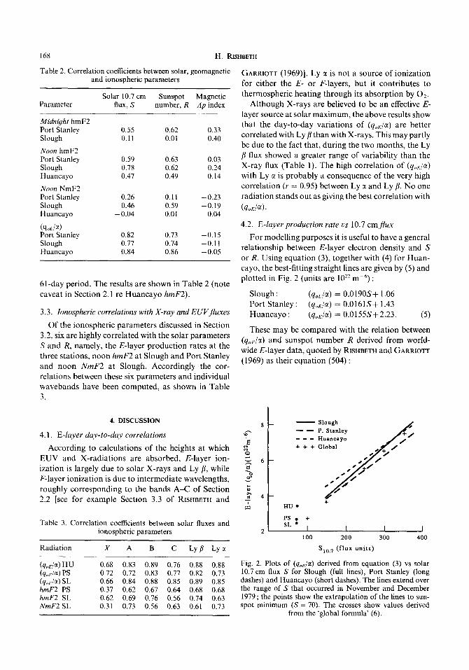
For modelling purposes it is useful to have a general

relationship between E-layer electron density and S or R. Using equation (3), together with (4) for Huan- cayo, the best-fitting straight lines are given by (5) and plotted in Fig. 2 (units are 10” mm”) :

Slough : (q&x) = O.O19OS+ 1.06 Port Stanley: (quE/u) = 0.016lSf 1.43 Huancayo : (q,&) = 0.0155S+2.23. (5)

These may be compared with the relation between

(q,e/cI) and sunspot number R derived from world- wide E-layer data, quoted by RISHBETH and GARRIOTT (1969) as their equation (504) :

S-

c --

‘E ___

:: +++

2 g 6-

‘D s ; 2 4- 2 HU 9

PS. + SL. ,

Slough

P. stan1cy

2’ I I I 100 200 300 400

S,,,, (flux units)

Fig. 2. Plots of (q,Ju) derived from equation (3) vs solar 10.7 cm flux S for Slough (full lines), Port Stanley (long dashes) and Huancayo (short dashes). The lines extend over the range of S that occurred in November and December 1979 ; the points show the extrapolation of the lines to sunspot minimum (S = 70). The crosses show values derived

from the ‘global formula’ (6).

Day-to-day ionospheric variations 169

(q,,&) = O.O180R+ 1.80 x 0.01945+0.71 (6)

in which the alternative equation involving S has been derived from the approximate formula used by RISHWTH and EDWARDS (1989) :

R = 1.08S-61. (7)

Equation (6). plotted as crosses in Fig. 2, is reason- ably consistent with the present data, though the slightly different slope might indicate a different ionospheric response to short-term and long-term variations of S. With an assumed (but reasonable) value of M = 2.5 x IO--‘” m3 s-‘, representing a compromise between the values of cc(NO+) and (0:) given by REES (1989), the mean of the three equations (5) gives

q,,, = (0.42S+39) x 10”m~3s-‘. (8)

This equation implies that, although the flux of solar ionizing radiation and the decimetric flux are related, they are not proportional to each other (there would be a substantial ionizing flux at S = 0, as mentioned in Section 3.1). The same is not true if the production rates were expressed in terms of the EUV fluxes; within the accuracy of the analysis, there is no significant residual ionization for zero flux. As expected, ,foE and Ap are uncorrelated.

The choice of n = 0.275 in equation (3) was made because it seems to give the best consistency in equation (5) between the results for the three stations. But it does not seem worth trying to determine n very precisely, given the limited accuracy of the data. As is well known, the departure from the idealized value of 0.25 is largely due to the vertical gradient of scale height H (it can be shown that n = 0.25(1 +dH/dh), e.g. NICOLET, 1951). This is partly offset by the effect of the temperature dependence of the electron-ion recombination coefficient CL

4.3. Day-to-day correlations qf!f2-layer electron den-

sity

In the simplest theoretical models of the F2-layer, the peak electron density NmF2 [or (foF2)*] is proportional to the ion production rate in the F2-layer. In practice the proportionality is greatly complicated by drifts and winds. In the present data, the correlation between NmF2 and solar activity is only mod- erate at Slough (winter), weak at Port Stanley (summer) and non-existent at Huancayo. Given the complexity of the processes that control the F2 peak, the lack of strong correlation is not surprising. The data give the impression that the midlatitude F2-layer is more solar-controlled in winter than in summer. The well-known negative correlation between NmF2

and Ap appears weakly in the data for the midlatitude stations.

No strong correlation is found between NmF2 and the EUV fluxes. The He II line (included in set B of Table 1) is sometimes regarded as a strong source of F-layer ionization, but its individual correlation with Slough NmF2 (r = 0.46) is weaker than that of the set B radiations as a whole (r = 0.56). Although general relationships between NmF2 and S (or NmF2 and R)

may be useful for modelling, it does not seem worth pursuing further the correlation of NmF2 with individual radiations.

4.4. Day-to-day correlations of F2-layer height

According to RISHBETH and EDWARDS (1989, 1990) the noon F2 peak lies approximately at a fixed pressure level. Its height therefore depends on the temperature profile in the thermosphere. Increasing solar activity raises the thermospheric temperature, thus causing thermal expansion which lifts the pressure level at which hmF2 is situated. One might then expect hmF2 to be positively correlated with the energy input due to solar EUV and X-rays. Table 3 confirms this, apart perhaps from the X-rays (which deposit their energy low down in the the~osphere)~ with no clear link to any specific EUV radiation. In terms of the indices S and R (Table 2), the correlation is strongest by day and also appears at night at Port Stanley (in summer). In winter (i.e. at Slough) the geomagnetic influence on hnzF2--also probably associated with heating and thermal expansion-is appreciable, but by day the geomagnetic effect is masked by the effect of solar activity.

At Huancayo, correlation between F2-layer parameters and solar activity is expected to be weak, because the equatorial F2-layer is largely controlled by electric fields. Although the MUF formula (2) is not reliable for the equatorial ionosphere, the significant correlations of MUF with S and R (r % 0.5) do suggest that even at Huancayo there is a systematic variation of layer height with solar activity.

A further study was made of correlations between the ionospheric parameters (noon NmF2, noon hmF2 and q,&). At all three stations, hmF2 and qDE/a are quite well correlated (r x 0.5). This is consistent with the expected relationship between energy input, thermospheric temperature and FZ-layer height. At Slough there is some correlation between NmF2 and both hmF2 and q,,/a (r z 0.4), consistent with the apparent solar control of the winter F2-layer.

4.5. FZ-layer height DS 10.7 cmjux

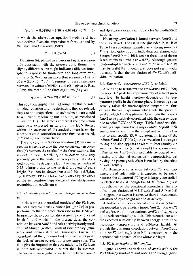
Figure 3 shows the variation of hmF2 with S for Port Stanley (midnight and noon) and Slough (noon

170 H. RISHBETH

300

- hm F2 Nov.-Dec. 1979 ___ hm F2 R & E 1990 - - MSIS Prcssurc levels , ,;

r0

,,,i 100 200 300

s 10,7 (flux units)

Fig. 3. Plots of hmF2 derived from equations (1) and (2) vs solar 10.7 cm flux S (full lines), compared to fixed-pressure levels according to the MSIS-86 model (long dashes) and the relations derived by RISHBETH and EDWARDS (1990) (short

dashes). Note the break in the height scale.

only). The best fitting relations (full lines) are as fol-

lows :

Port Stanley (midnight) : hmF2 = 0.53S+ 320 [km] Port Stanley (noon) : hmF2 = 0.6OS+265 [km] Slough (noon) : hmF2 = OS2S+ 195 [km].

(9)

The short dashes in Fig. 3 show the relations derived by RISHBETH and EDWARDS (1990) and the long dashes show the variation of height of constant pressure levels derived from the MSIS86 model (HEDIN,

1987), that is, 2 and 20 PPa for Port Stanley midnight and noon, 25 PPa for Slough noon. The three Slough noon curves agree well. For Port Stanley the agreement is only fair for the midnight curves; the MSIS and R&E model values rise more steeply with S than do the 1979 data. For noon at Port Stanley, agreement is poor ; the 1979 values of hmF2 are 3&40 km above those derived from MSIS and the large slope derived by RISHBETII and EDWARDS seems unrealistic. F-layer

modelling in southern latitudes clearly needs to be

improved.

5. CONCLUSION

The large variations of solar activity in November

and December 1979 provide an excellent opportunity to study the day-to-day response of the ionosphere. The period is almost free of complications due to seasonal changes and geomagnetic activity (Section 1) and is well covered by solar flux data (Section 2.2).

However, the present work is not intended as a study of solar physics and the relations between different solar emissions and indices have been discussed only to the extent needed to provide background information for the solar-ionospheric analysis. Much longer datasets are available for purely solar studies ; for example DONNELLY (1987) has studied the auto- correlations and cross-correlations of several solar emissions during 1977-1980.

At the three ionosonde stations chosen for the

analysis (Slough, Huancayo and Port Stanley), the day-to-day variations of the E-layer critical frequency

foE and the height of the F2 peak are well correlated with solar indices (10.7 cm flux and sunspot number)

and EUV fluxes, with correlation coefficients of 0.7- 0.9 (Tables 2 and 3). Of the radiations believed to be important in ionizing the E-layer, the H Lyman b flux

is better correlated with foE than is the X-ray flux at O.lWJ.8 nm (Section 4.2). The variations of foE with solar 10.7 cm flux are consistent with previous results (Section 4.2).

No other significant information about the iono-

spheric role of particular solar radiations emerged from the analysis. Only for the winter station (Slough)

was any correlation found between solar activity and F2-layer electron density (Section 4.3) ; no strong correlation would in fact be expected, the F2 peak being largely controlled by winds and drifts.

The correlations between solar parameters and

noon hmF2 (Sections 3.2, 3.3, 4.4) are mostly in the range 0.6-0.75. They support the idea that the F2 peak lies at a constant pressure level (at a given local time). Increasing solar activity heats and expands the thermosphere, causing the F2 peak to rise. However, the best fits of hmF2 vs 10.7 cm flux agree only mod- erately well with previous work and with relationships derived from the MSIS model (Section 4.5). It probably asks too much of MSIS to expect a good rep- resentation of thermospheric changes at a time of rapidly varying solar activity.

HEDIN (1984) studied the correlation between S,

EUV fluxes, Ca plage emissions and other solar par-

ameters with thermospheric density and temperature. He found that day-to-day correlations, though high

(mostly 0.854.95), were less than the correlations of the 81-day means (mostly 20.95). HIN~~RE~ER (198 I) also found that the correlations of EUV emissions with S are better for 81-day means than for the daily values. The present results do not conflict with this conclusion, but show that day-to-day correlations are high even when solar activity is varying rapidly.

As for further work: it would be worth using the SC # 2 I OBS solar datafile (used in this work) for a 3.5 y comparison of day-to-day and longer-term variations in the ionosphere. Due regard should be paid to the longer-term calibration of the data and it would be e.wntiaf to remove seasonal and geomagnetic effects in the ionospheric data. The present results,

though confined to a two-month period, have impli- cations for ionospheric modelling. ~urne~ca~ simu-

lations with a the~osphe~c general circulation model might provide an interesting picture of this extraordinary period.

Acknowledgements-Ionospheric data for this study were obtained from the WDC-Cl for Solar-Terrestrial Physics at the Rutherford Appleton Laboratory, Chilton, U.K. Solar- geophysical indices were taken from publications of the WDC-A for Solar-Terrestrial Physics, Boulder, Colorado. The author is grateful to WDC staff for their help, to Dr R. F. Donnelly for a valuable discussion and for supplying copies of solar data and to the referees for helpful comments. The work was begun during a sabbatical term at the Center for Space Physi~s~Bostnn University and was also supported by the U.K. Science and engineering Research Council.

Day-to-day ionospheric variations 171

REFERENCES

BOUWEK S. D., DONNELLY R. F., FALCON J., QUINTANA A. and CALDWELL C.

1982 NOAA Tech. Memo. ERL SEL-62, National Oceano- graphic and Atmospheric Administration, Boulder, Colorado.

DONNELLY R. F. DONNELLY R. F., HIN~REGGER H. E. and HEATH D. F. DUDENE:Y J. R. HEWN A. E. HEUIN A. E. HINTIERKGER H. E. HINTEREGG~R H. E., FLIKUI K. and GUON B. R. MORONW M. J.

1987 Solar Phys. 109, 37. 1986 J. geophys. Res. 91, 5567. 1983 J. atmos. terr. Phys. 45, 629. 1984 J. geophys. Res. 89,9828. I987 J. geophys. Res. 92,4649. 1981 A&). Space Res. 1, 39. 1981 Geophys. Res. Lett. 8, 1147. 1965 ~u~f~~o~ Figures (2nd Edition). Penguin, Harmonds-

worth, U.K. M~JGGLETON L. 1972 Nfc0r.m’ M 1951 REES M. H. 1989

RfSHRETH H. and EDWARDS R. 1989 RISHBETH H. and EDWARDS R. 1990 RISHUETH H. and GARRIOTT 0. K. 1969

SHIMAZAKI T. 1957

J. atmos. ten-. Phys. 34, 1385. J. atmos. ferr. Phvs. I, 141. Appendix 5. Phy& and Chemistry of the Upper Atmos-

phere, Cambridge University Press, Cambridge, U.K. J. atmos. terr. Phys. 51, 321. Radio Sci. 25, 1.57. Introduction to ionospheric Physics. Academic Press,

New York, U.S.A. J. Radio Res. Luhs 4, 57.

day-to-day ionospheric variations in a period of high solar activity

Documents