daily life and demand: an analysis of intra-day variations

ORIGINAL ARTICLE

Daily life and demand: an analysis of intra-day variationsin residential electricity consumption with time-use data

Aven Satre-Meloy & Marina Diakonova &

Philipp Grünewald

# The Author(s) 2019

Abstract Demand-side flexibility has been suggestedas a tool for peak demand reduction and large-scaleintegration of low-carbon electricity sources. Deeperinsight into the activities and energy services performedin households could help to understand the scope andlimitations of demand-side flexibility. Measuring andEvaluating Time- and Energy-use Relationships(METER) is a 5-year, UK-based research project andthe first study to collect activity data and electricity usein parallel at this scale. We present statistical analyses ofthese new data, including more than 6250 activitiesreported by 450 individuals in 173 households, and theirrelationship to electricity use patterns. We use a regular-ization technique to select influential variables in regres-sion models of average electricity use over a day and ofdiscretionary use across 4-h time periods to compareintra-day variations. We find that dwelling and appli-ance variables show the strongest associations to aver-age electricity consumption and can explain 49% of thevariance in mean daily usage. For models of 4-h averageBde-minned^ consumption, we find that activity vari-ables are consistently influential, both in terms of coef-ficient magnitudes and contributions to increased modelexplanatory power. Activities relating to food prepara-tion and eating, household chores, and recreation showthe strongest associations. We conclude that occupantactivity data can advance our understanding of the

temporal characteristics of electricity demand and in-form approaches to shift or reduce it. We stress theimportance of considering consumption as a functionof time of day, and we use our findings to argue that amore nuanced understanding of this relationship canyield useful insights for residential demand flexibility.

Keywords Household electricity consumption . Peakdemand .Demand flexibility .Time-usedata .Regressionanalysis

Introduction

The residential sector is the largest end user of electricityin the UK, accounting for 45% of total consumption in2017 (BEIS 2018). It is also responsible for up to 50%of national peak demand, during which time electricityprovision is especially costly and carbon-intensive(Ofgem 2010). As evidenced by the share of generationfrom renewables increasing to over 29% in 2017, theUK’s electricity system is increasingly low-carbon, yetmuch more ambition is needed to achieve national cli-mate goals in the next decades (BEIS 2018).

The UK’s 2017 Clean Growth Strategy sets forth aset of policies and proposals to further accelerate thedeployment of low-carbon energy while maintainingincreased economic growth (BEIS 2017). One of theproposals, the BSmart systems plan,^ aims to help con-sumers use energy more flexibly. Energy storage willsupport integration efforts as the UK pursues rapiddeployment of renewable energy, but demand flexibility

https://doi.org/10.1007/s12053-019-09791-1

A. Satre-Meloy (*) :M. Diakonova : P. GrünewaldEnvironmental Change Institute, University of Oxford, SouthParks Rd, Oxford OX1 3QY, UKe-mail: [email protected]

Energy Efficiency (2020) 13:433–458

Published online: 24 April 2019

http://crossmark.crossref.org/dialog/?doi=10.1007/s12053-019-09791-1&domain=pdf

can reduce the cost of integration and storage require-ments for low-carbon energy systems (NationalInfrastructure Commission 2016).

Understanding how to make demandmore flexible inthe residential building sector requires a more detailedinvestigation of what electricity is used for in house-holds (Grunewald and Diakonova 2018a; Powells et al.2014). Time-use data is increasingly used for modelingelectricity consumption, but these analyses often usesimulated activity data and proxies for electricity con-sumption, such as household expenditure data, whichrequires assumptions about the link between time-usedata and electricity consumption patterns. In somecases, these models are validated against real consump-tion data, though the validation sample sizes are in the10–20 household range (Richardson et al. 2010; Widénet al. 2009;Widén andWäckelgård 2010). Even as time-use data has been more recently incorporated into thesemodels, however, there remains a notable gap in theliterature of empirical studies on how occupant activitiesinfluence the temporal aspects of demand (Anderson2016; Anderson and Torriti 2018; Grunewald andDiakonova 2018b).

In this paper, we aim to contribute to filling this gapby constructing regression models of original survey,time-use, and electricity consumption data for 173 UKhouseholds collected as part of an ongoing study. Wetest the extent to which socio-demographic, dwelling,appliance, and activity data can explain variations inintra-day household electricity use, from 5 p.m. until 9p.m. on the following day. We then compare the effectsof reported time-use activities in households throughoutthe day by dividing the day into six equal 4-h periods.

We aim to understand whether and how the inclusionof categorized activity data improves models of house-hold electricity consumption. We investigate how dif-ferent categories of activities are associated with elec-tricity consumption during different times of day, andwe consider how this knowledge can inform efforts toenhance demand-side flexibility and enable more andless costly integration of renewable energy sources.

The paper is organized as follows: In the BLiteraturereview^ section, we present a brief review of the flexi-bility and household electricity modeling literature, in-cluding both determinants of household electricity con-sumption and the use of time-use data in energy model-ing. In the BData and methodology^ section, we presentour methodology for collecting household electricityand time-use data in parallel. The BResults^ section

presents results of full-day and 4-h models of averageelectricity consumption. In the BDiscussion^ section, wediscuss the implications of our findings, and in theBConclusions^ section, we conclude.

Literature review

Demand-side flexibility

Flexibility has been defined in the energy demand liter-ature as the ability for consumers to change how, when,and where energy is used—a shift in focus from themagnitude of overall consumption to the timing of de-mand (Powells et al. 2014; Torriti et al. 2015). Weconceive of it here simply as Ba potential to changepower at a certain rate (Watt/hour)^ (Grunewald andDiakonova 2018a, p. 59). While much of the focus indemand-side energy research has been on reducing de-mand through energy efficiency, as the energy systembecomes increasingly supplied by variable, low-carbongeneration, flexibility becomes increasingly importantfor balancing supply and demand. The potential respon-siveness of demand, or its ability to shift in time tomatch high generation from renewables or to flattendemand during peak periods, is essential for minimizingthe costs of transitioning to a low-carbon power system(Strbac et al. 2012).

Demand-side response (DSR) refers to measures thatprovide flexibility to the energy system by shifting orreshaping energy loads. McKenna et al. (2017) conceiveof DSR as a three-dimensional space includingBtechnology change,^ Bservice expectation change,^and Bactivity change.^ The technology change dimen-sion refers to an automated or remotely controlled shiftin energy use, for example, a smart fridge that delivers aresponse without affecting the energy service delivered.The authors note this has been the main form of DSRthat has been tested in energy models given the relativeease of simulating such technology changes. BServiceexpectation change^ refers to shifting occupants’ ex-pected level of energy service from an appliance ortechnology (i.e., the thermostat set-point), while anBactivity change^ requires a shift in either the timingor type of activity and relies on more active behavioralchanges among energy users.

Grünewald and Diakonova (2018a) more broadlydifferentiate these dimensions of DSR as Bapplianceled^ and Bactivity led.^ Among Bactivity led^ DSR are


several different types of shift mechanisms: activityshifts, or changing the timing of an activity; substitutingpractice, which does not reorder activities in time butinstead substitutes an energy-intensive activity for onethat is not (e.g., having a cold rather than hot meal);substituting metabolic energy, such as mixing dough byhand rather than with an electric mixer; or changing thepractitioner, which might entail going out for dinnerrather than cooking at home.

Recent research has begun to investigate the DSRpotential of these and similar types of measures, but stilllittle is known about both the mechanisms by whichelectricity consumption patterns can be reshaped and thedifferent constraints or motivating factors that can re-shape them. A review of major DSR trials in the UKfound that residential customers are responsive to eco-nomic incentives to shift demand but that the size of theshift can vary significantly (DECC 2012). The reportnotes several areas where findings were inconclusive.These include the responsiveness of vulnerable and low-income customers, the impact of non-economic signals,and detailed information on the way consumers shifttheir usage in response to incentives.

Further empirical work on the flexibility of house-hold activities includes research that qualitativelyassessed the likelihood of certain practices being per-formed during peak hours (4–8 p.m.) (Powells et al.2014). This study found a very high or high likelihoodof TV watching, cooking, computer/Internet use, anddish washing during these hours, with lesser frequenciesof laundry, ironing, vacuuming, and bathing. More in-sight into the types of activities happening during peakperiods and their contributions to electricity demand canhelp identify those that are best suited for DSR.

But how well Bsuited^ an activity is for shifting is notthe same as how Bflexible^ it might be. Torriti et al.(2015) stress this point by developing a "FlexibilityIndex" composed of five separate indices (synchroniza-tion, variation, non-shared activities, active home occu-pancy, and spatial mobility). These component indicesare calculated for five time periods throughout the dayfor a sample of 153 respondents, and the findings showthat morning peak times feature high levels of synchro-nization and shared activities but low variation in activ-ities. Evening peak times show less synchronization buthigher spatial mobility and variation in activities.

Demand-side flexibility is complex and is difficult tomeasure empirically. It is likely that socio-demographic,dwelling, appliance ownership characteristics, and

activity patterns bear a strong relationship to both thetypes of DSR that can take place in homes as well as thecapacity of households to participate in DSR programs.Several different approaches have been developed tobetter understand these relationships in order to informmore effective DSR. The following sections reviewthese approaches in the context of research on electricitydemand modeling and incorporating time-use data inthese models.

Household electricity demand: models and determinantsof use

The literature on quantitative approaches to model andunderstand key socio-technical determinants of electric-ity use in households is expansive. Previous studiesemploy both top-down and bottom-up approaches.Top-down approaches consider how national-level data,such as characteristics of the housing stock and macro-economic factors, influence electricity consumption,while bottom-up approaches use detailed household-level data on dwelling characteristics and occupantsocio-demographics to identify the primary drivers ofelectricity consumption for a sample of households andthen extrapolate these findings to the wider population(Swan and Ugursal 2009). Studies are also varied inhow they measure household electricity use, in somecases considering average annual consumption valueswhile in others studying daily or hourly consumption.

A recent comprehensive review of the socio-demo-graphic, dwelling, and appliance-related determinants ofhousehold electricity consumption undertaken by Joneset al. (2015) shows that no fewer than 62 factors havebeen found to affect household electricity consumption.Twenty of these are consistently found to have a signif-icant, positive correlation with electricity use(Bconsistently^ is defined by the authors as showing astatistically significant relationship in more than threestudies). The socio-demographic factors include numberof occupants, presence of teenagers, household income,and disposable income. The impact of occupant age,education level, and tenure type is inconclusive in thestudies reviewed. The dwelling factors that are influen-tial include dwelling age, dwelling type, number ofrooms, total floor area, and ownership of electric spaceheating and cooling systems. Appliance factors includeownership of a desktop computer, television, electricoven, refrigerator, dishwasher, washing machine, and

Energy Efficiency (2020) 13:433–458 435

tumble dryer, as well as the overall number of appli-ances owned.

Huebner et al. (2016) confirm many of these findingsin one of the few representative studies of electricityconsumption in the UK residential sector. Using datafrom a sample of 845 English households from 2011 to2012, they find that models containing only applianceownership and use factors explain 34% of the variancein non-heating annual electricity consumption, whereasmodels containing socio-demographic variables explainonly 21%, and models containing dwelling and otheroccupant variables are poor in explaining electricity use.Their model combining these factors shows that dwell-ing floor area, number of occupants, wet applianceownership, and hours of TV watched per day are statis-tically significant predictors of annual consumption.

As our paper focuses specifically on factors affectingintra-day variations in electricity use, a brief review offindings from studies with a similar focus is includedhere. The number of these studies is fewer than thoseincluded in the review discussed above because in muchof the previous research, advanced metering data wasnot as available or accessible. With the growth of smartmeter adoption, however, these data and studies inves-tigating them are becoming increasingly common.

In general, this body of work suggests that applianceownership and usage factors have stronger relationshipswith variations in consumption than socio-demographicand dwelling factors. In a study monitoring 27 UKresidential buildings’ electricity consumption at 5-minintervals for a period of 2 years, Firth et al. (2008) findthat an observed increase in usage between years isprimarily attributable to increases in the consumptionof standby appliances, such as televisions and otherconsumer electronics, and Bactive^ appliances, such askettles, washing machines, electric showers, andlighting.

McLoughlin et al. (2012) study the effect of dwellingand occupant characteristics for a representative sampleof 4200 Irish dwellings on several dependent variables,including total electricity consumption over a 6-monthperiod, mean daily maximum demand over that period,electrical load factor (ratio of daily mean to daily max-imum electrical demand), and timing of peak demand.They find that several dwelling and socio-demographicfactors, such as number of bedrooms, type of dwelling,and head of household age, are significant in explainingload factor variations (i.e., those that are Bpeakier^ orBflatter^). They also find that timing of peak demand is

mostly driven by variables measuring reported appli-ance ownership and use, especially dishwashers, electricpower showers, televisions, and desktop computers.Notably, the models are less able to explain load factorand timing of peak demand than total consumption andmean daily maximum demand. Key explanatory factorsfor understanding variations in electricity consumptionat different times of day may therefore be missing in themodels.

Exploiting a similar smart meter data set from theIrish Commission for Energy Regulation (CER), Ander-son et al. (2016) examine the links between half-hourlyelectricity consumption data and household characteris-tics for the purpose of assessing the feasibility of usinghigh-resolution electricity data to infer household char-acteristics to supplement census-taking efforts. Theyconstruct multi-level regression models to analyze nu-merous Bprofile indicators^ that describe the temporalcharacteristics of load profiles, such as base load, meanload, 97.5th percentile load (as a proxy for peak load),and several other temporal parameters. Their resultsshow that several household characteristics, such asnumber of occupants, household income, and presenceof children, are useful predictors of several of theseBprofile indicators,^ especially those measuring overallmagnitude of consumption.

Kavousian et al. (2013) examine structural and be-havioral determinants of daily maximum and minimumdemand for a data set of 10-min interval electricityreadings and an extensive household survey of 1628US dwellings in California. The study was non-random and had a sample biased toward high-incomeand well-educated participants. They find that whiledaily minimum consumption is influenced most byweather, location, and physical characteristics of thebuilding, such as size and type of home, daily maximumdemand is influenced by high-consumption, intermittentappliances, such as electric water heaters or tumbledryers. The authors note the clear difference in theirresults between drivers of daily minimum and maxi-mum demand, explaining that peak demand is moredependent on the activity patterns that lead to use ofhigh-consumption appliances. Minimum demand isdriven primarily by locational and physical characteris-tics of the dwelling.

Several recent papers have aimed to investigatesocio-demographic and physical dwelling determinantsof whole load profile shapes rather than average valuesof electricity consumption across varying time periods


(McLoughlin et al. 2015; Rhodes et al. 2014; Viegaset al. 2016). These studies take an alternative approachby first clustering load profiles into representative pro-file classes and then using logistic regression to deter-mine factors influencing membership in different loadprofile classes. While this is a different approach thanthe one used in this paper and in the studies reviewedabove, it achieves a similar aim. The findings from thesestudies indicate that variables such as working fromhome, time spent watching television, age, and owner-ship of dishwashers and washing machines are mostimportant for explaining the shape of a household’sdaily electrical load profile.

The literature investigating highly resolved variationsin residential electricity consumption is growing along-side the availability of data, but many of the resultsdiscussed here are dependent on the sample nature andsize and not necessarily generalizable to wider popula-tions. It is also important to consider the climatic andsocial contexts in which these studies are undertaken, asthese likely influence their findings.

Incorporating time-use data in models of electricityconsumption

Social scientists have long researched the dynamics ofdaily life through studies of how people spend theirtime. Longitudinal studies of thousands of householdshave investigated questions of historical changes in timeuse and how these relate to trends in technological andsocial change (eurostat 2009; Gershuny 2008; U.S.Bureau of Labor Statistics 2018). Research in energydemand modeling has acknowledged the need to takeaccount of the timing of household activities in order tomore accurately represent electricity demand (Torritiet al. 2015). In the last decade, occupant activity datafrom time-use studies has been increasingly incorporat-ed into high-resolution models of residential electricityconsumption (Torriti 2014). These studies involve vary-ing approaches for incorporating time-use data. In somestudies, probabilistic simulations are used to developmodels of active occupancy, occupant activity se-quences, and appliance usage that are predictive ofelectricity load curves (Ellegård and Palm 2011;Richardson et al. 2010; Widén et al. 2009). In others,changes in electricity consumption over decades arelinked to changes in time-use and household expendi-ture data, often using decomposition analysis, whichattributes changes in these factors to overall changes in

electricity use (De Lauretis et al. 2017; Jalas andJuntunen 2015; Sekar et al. 2018). In many of thesestudies, models and results are validated with actualconsumption measurements from a small sample ofhouseholds (McKenna and Thomson 2016; Widénet al. 2009).

While this literature shows varying results for thelinks between time use and electricity consumption,some common themes emerge. Mealtimes and relatedactivities are consistently found to be high-consumptionactivities (De Lauretis et al. 2017; Druckman et al. 2012;Jalas and Juntunen 2015). Studies also find evidencethat housework and personal time are energy-intensiveactivities (Palmer et al. 2013; Widén et al. 2009). Un-surprisingly, sleeping and resting are low-consumptionactivities (Druckman et al. 2012; Jalas and Juntunen2015), whereas recreational activities can be either highor low energy depending on whether they involvetelevisions and computers or reading and socializing.In terms of the temporal shifts in the timing of UK peakdemand over the past 40 years, Anderson and Torriti(2018) find that this is mostly due to changes in food-related activities, in part due to changes in personal careand housework shifts, and little to do with changes inmedia use.

Using the specific case of laundry practices in theUK, Anderson (2016) highlights the role of societalchange in time shifts for energy-using activities. In-creases in labor market participation by more femalesin society is likely partially responsible for shiftinglaundry energy demand into weekday mornings andevening peak times but also into Sunday mornings,which are less problematic for providing energy. Theauthor concludes that more analyses of the changes toroutine energy-using practices are necessary forassessing the value of various demand responsestrategies.

A review of time-use modeling of electricity demandundertaken by Torriti (2014) identifies five limitations inthe literature. First, time-use data must be aggregatedacross large numbers of households to be statisticallysignificant. Second, time-use data are often sampledthroughout the year, whereas peak electricity eventsoften happen on specific days, such as during tempera-ture extremes or national events. Third, the low frequen-cy of large time-use surveys means the data quicklybecome outdated. Fourth, the timing of occupancy andtypical activities in developed countries is less variablethan other factors that influence consumption, such as


weather or appliance design. Fifth, modeling multiple-person households using time-use data, especially formodeling occupancy patterns, is muchmore challengingthan for single-person households, which was con-firmed empirically by Grünewald and Diakonova(2018b). The fourth point, however, is contested.Tabbone et al. (2016) found that even within countries,cultural differences in time-use can affect load profiles.

To these limitations, McKenna et al. (2017) addseveral additional failings of time-use demand models.First, they note that time-use studies were not originallydesigned for the purpose of modeling energy use, andthey thus do not differentiate between Benergy-intensive^ or Blow-energy^ alternatives of the sameactivity. Meal time is a good example, as this can varyfrom relatively low energy (cold meal preparation) tovery energy intensive (oven and electric hob use). Sec-ond, time-use data do not account for overlapping orBbundled^ activities, such as those that might occurduringmulti-tasking. Third, the typical 10-min reportingwindow for activities may not capture energy-relevantyet shorter duration activities, such as boiling the kettle.

This study addresses the limitations highlighted inthese two reviews through a new approach to collectingtime-use data. To the authors’ knowledge, this is the firststudy to collect time-use data and electricity readingsdirectly from households in parallel at this scale. Thisresearch contributes to an emerging focus within energydemand studies on not only the magnitude but also thetiming of electricity consumption in households andhow it is influenced both by numerous socio-demographic and dwelling factors that have been stud-ied in previous research, as well as by the activities ofoccupants, which may contribute additional insights fordetermining the timing of electricity use in homes andthe potential for shifting these activities to provide moreflexibility to the energy system.

Data and methodology

Data collection

Electricity readings and activity records are collectedfrom UK households as part of an ongoing study(Grünewald and Layberry 2015). Participation is volun-tary, and participants are recruited online, via radio, andthrough campaigns at selected community events. An

incentive for participation is the chance to win a year’sworth of free electricity.

When registering for the study, participants completea survey wherein they provide detailed socio-demographic information along with data on dwellingcharacteristics and appliance ownership. Participatinghouseholds are sent a parcel prior to their chosen date,which includes an electricity recorder, activity re-corder(s), and an instruction booklet. The study encour-ages all household members over the age of eight toparticipate.

Participants are instructed to attach the electricityrecorder below the household’s electricity meter. Theelectricity recorder collects readings every second for28 h, from 5 p.m. on their chosen day until 9 p.m. thefollowing day. This study length is chosen in order tocapture two typical peak demand periods and becausethe electricity recorders have a battery life of around28 h per charge. Fuel type used for heating and cookingappliances is collected in the household survey.

Activities are recorded with a dedicated app pre-installed on individual devices. The app presents sixoptions per screen that guide participants throughrecording their activities, starting with the locationand concluding with the number of people partakingin the activity and one’s enjoyment of it. Askingabout enjoyment was found to increase participantretention in previous time-use research (Gershunyand Sullivan 2017). Figure 1 shows an example ac-tivity entry sequence. In contrast to paper-based time-use diaries (eurostat 2009), the app can guide partic-ipants to select energy-relevant details, such as appli-ance use, allowing for detailed descriptions of activ-ities. Instead of capturing the duration of activities, aswas done in previous time-use studies, the app re-cords activities reported instantaneously. Users canrecord multiple activities in sequence and are alsogiven an option to record the Bend^ of activities.While users are encouraged to report activities whenthey actually occur, entries can be made retrospec-tively and into the future. One test of validity forreporting accuracy suggests around 80% of activityrecords for boiling the kettle are reported within10 min of the activity itself (see Grünewald andDiakonova (2018b) for more details). More detailsabout the functionality of the app is discussed inGrünewald et al. (2017), and a description of the datastorage and handling procedures can be found inGrünewald and Diakonova (2019).


Study sample

The study sample consists of 173 households and 447individuals who together reported 6265 activities. Theprocess for determining inclusion in the subsequentanalyses is as follows:

& Household that own solar PV are excluded due toconcerns about the validity of electricity readings.

& Households that did not complete the full survey areexcluded. The small occurrence of missing data(11% or 23 cases) did not warrant more complexhandling, such asmultiple imputation, so these casesare deleted listwise.

& Electricity readings below 20 W are excluded fromdaily and 4-h averages, as this signals a failure toattach the electricity recorder properly.

& Activities that were reported either before the elec-tricity meter starts recording or after it stops areexcluded. Similarly, activities that are reported inan hour where a valid electricity reading is missingare excluded.

& Only activities reported in the home are included,since we are interested in those activities that have adirect influence on household electricity consumption.

Socio-demographic, dwelling, and appliance variables

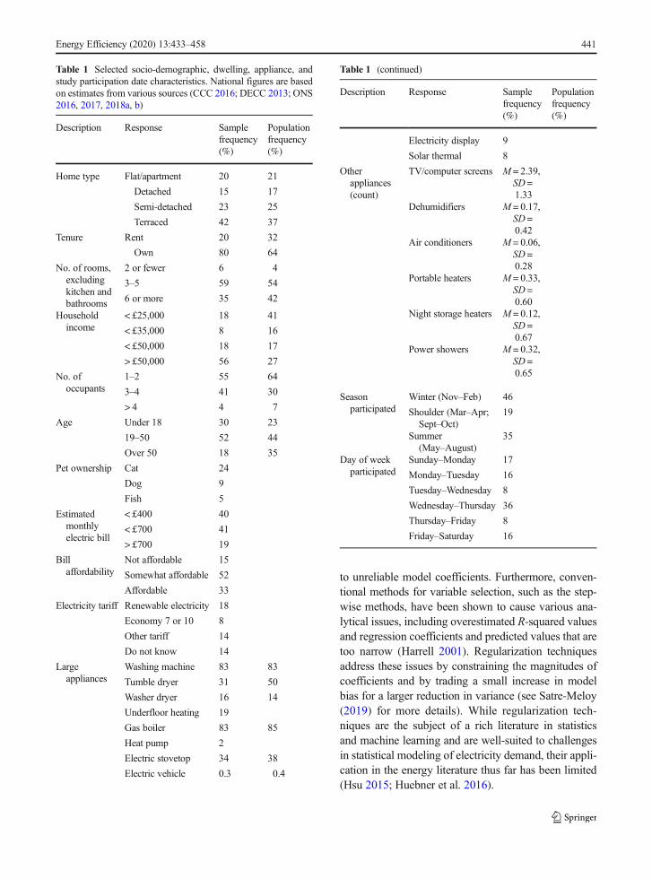
The household survey includes questions on occupantsocio-demographics, physical dwelling characteristics,and appliance ownership. In previous studies, thesehave shown to have the strongest associations withresidential electricity consumption in the UK (Huebneret al. 2016; Jones and Lomas 2016;Wyatt 2013). Table 1presents frequencies and descriptive statistics for thesevariables for both the sample and the wider UK popu-lation (where available). Categorical variables are dum-my coded prior to analysis, and reference categories arebolded in Table 1. Estimated monthly electric bill mea-sures participants’ estimate of their electricity expendi-ture. While we would expect this to have a positiveassociation to average daily electricity consumption,we suspect that monthly estimates on expenditure mightvary widely from day-to-day variations in consumption.We include it in our analyses to understand how welloccupant estimates of electricity consumption do in factpredict actual average daily consumption values.

The study is voluntary, and the sample is not fullyrepresentative of the general UK population. Selectionbiases include an underrepresentation of renters, low-income groups, and the elderly. Gas boiler ownership isslightly underrepresented, suggesting a higher preva-lence of all-electric heating in the sample. These biasesare likely to influence both overall consumption as wellas the timing of demand, which is why we cautionagainst overgeneralizing from these results.

Table 1 also lists the distributions of season and dayof week that households participate. A majority ofhouseholds (57%) participate during the winter season(November–February). Data collection is focused onthis season because it coincides with UK annual peakdemand (DECC 2014). Households are recruited to startthe study on a weekday, though given the study periodspans 2 days, 22% of the sample starts on a Friday andcompletes the study on a Saturday. We do not createseparate models for season or day of week in order topreserve the sample size across models, but we doinclude these as candidate variables during model selec-tion, which is further explained below.

Activity variables

The app pre-codes activities, following the HarmonizedEuropean Time-Use Studies (HETUS) standards. Forthis analysis, activities are grouped into seven catego-ries, which have become common in time-use research(Ellegård et al. 2010; Lader et al. 2006; Stankovic et al.2016). Examples of activities that fall into each categoryare shown in Table 2.

In the following analyses, activities are aggregatedacross household members so that each household has atotal count, or frequency, for each activity category.Table 2 presents descriptive statistics for each activitycategory for the sample.

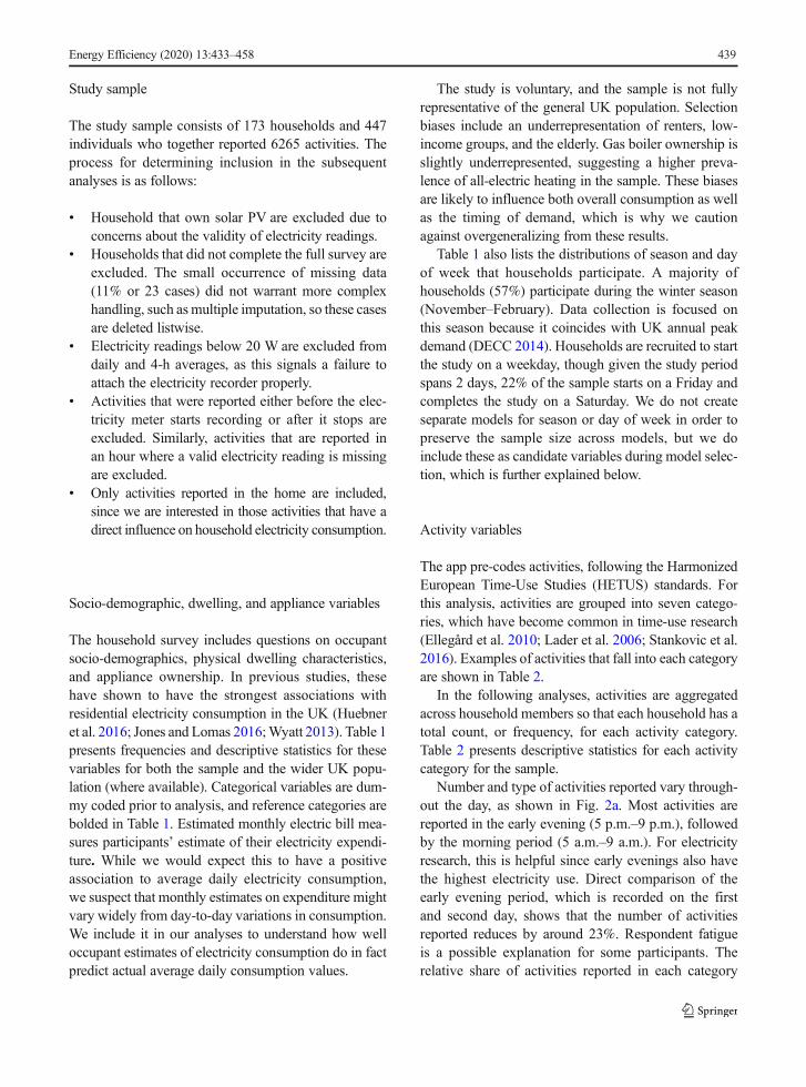
Number and type of activities reported vary through-out the day, as shown in Fig. 2a. Most activities arereported in the early evening (5 p.m.–9 p.m.), followedby the morning period (5 a.m.–9 a.m.). For electricityresearch, this is helpful since early evenings also havethe highest electricity use. Direct comparison of theearly evening period, which is recorded on the firstand second day, shows that the number of activitiesreported reduces by around 23%. Respondent fatigueis a possible explanation for some participants. Therelative share of activities reported in each category


remains similar, however, so we do not expect this tobias the second 5–9 p.m. model.

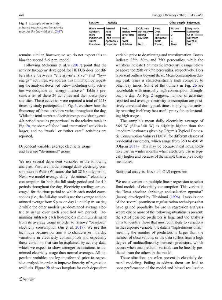
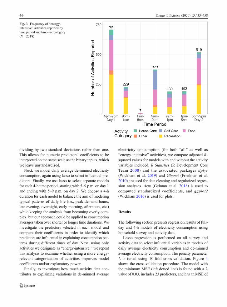
Following Mckenna et al.’s (2017) point that theactivity taxonomy developed for HETUS does not dif-ferentiate between Benergy-intensive^ and Blow-energy^ activities, we address this limitation by repeat-ing the analysis described below including only activi-ties we designate as Benergy-intensive.^ Table 3 pre-sents a list of these 26 activities and their descriptivestatistics. These activities were reported a total of 2218times by study participants. In Fig. 3, we show how thefrequency of these activities varies throughout the day.While the total number of activities reported during each4-h period remains proportional to the relative totals inFig. 2a, the share of Bfood^ and Brecreation^ activities islarger, and no Bwork^ or Bother care^ activities arereported.

Dependent variable: average electricity usageand average Bde-minned^ usage

We use several dependent variables in the followinganalyses. First, we model average daily electricity con-sumption inWatts (W) across the full 28-h study period.Next, we model average daily Bde-minned^ electricityconsumption for both the full study period and for 4-hperiods throughout the day. Electricity readings are av-eraged for the time period to which each model corre-sponds (i.e., the full-day models use the average and de-minned average from 5 p.m. on day 1 until 9 p.m. on day2 while the other models use de-minned average elec-tricity usage over each specified 4-h period). De-minning subtracts each household’s minimum demandfrom its average usage in order to remove Bbaseload^electricity consumption (Jin et al. 2017). We use thistechnique because our aim is to characterize intra-dayvariations in electricity consumption and especiallythose variations that can be explained by activity data,which we expect to show stronger associations to de-minned electricity usage than normal averages. All de-pendent variables are log-transformed prior to regres-sion analysis in order to improve linearity of regressionresiduals. Figure 2b shows boxplots for each dependent

variable prior to de-minning and transformation. Boxesindicate 25th, 50th, and 75th percentiles, while thewhiskers indicate 1.5 times the interquartile range belowor above the 25th or 75th percentiles, respectively. Dotsrepresent outliers beyond these. Mean consumption dur-ing peak times is characteristically high compared toother day times. Some of the outliers in Fig. 2b arehouseholds with unusually high consumption through-out the day. As Fig. 2 suggests, number of activitiesreported and average electricity consumption are posi-tively correlated during peak times, implying that activ-ity reporting itself may be a useful proxy for understand-ing high usage.

The sample’s mean daily electricity average of565 W (SD = 340 W) is slightly higher than theBmedium^ estimates given by Ofgem’s Typical Domes-tic Consumption Values (TDCV) for different classes ofresidential customers, which range from 350 to 490 W(Ofgem 2017). This may be because most householdstake part in winter months when electricity use is typi-cally higher and because of the sample biases previouslymentioned.

Statistical analysis: lasso and OLS regression

We use a variant on multiple linear regression to selectfinal models of electricity consumption. This variant isthe Bleast absolute shrinkage and selection operator^(lasso), developed by Tibshirani (1996). Lasso is oneof the several prominent regularization techniques thathave gained popularity for use in regression analyseswhere one or more of the following situations is present:the set of possible predictors is large and the analysisaims to identify those that most contribute to variationsin the response variable; the data is Bhigh-dimensional,^meaning the number of predictors is larger than thenumber of observations; or the data suffers from a highdegree of multicollinearity between predictors, whichoccurs when one predictor variable can be linearly pre-dicted from the others in the model.

These situations are often present in electricity de-mand modeling. Failing to address them can lead topoor performance of the model and biased results due

Fig. 1 Example of an activityentrance sequence on the activityrecorder (Grünewald et al. 2017)


to unreliable model coefficients. Furthermore, conven-tional methods for variable selection, such as the step-wise methods, have been shown to cause various ana-lytical issues, including overestimated R-squared valuesand regression coefficients and predicted values that aretoo narrow (Harrell 2001). Regularization techniquesaddress these issues by constraining the magnitudes ofcoefficients and by trading a small increase in modelbias for a larger reduction in variance (see Satre-Meloy(2019) for more details). While regularization tech-niques are the subject of a rich literature in statisticsand machine learning and are well-suited to challengesin statistical modeling of electricity demand, their appli-cation in the energy literature thus far has been limited(Hsu 2015; Huebner et al. 2016).

Table 1 Selected socio-demographic, dwelling, appliance, andstudy participation date characteristics. National figures are basedon estimates from various sources (CCC 2016; DECC 2013; ONS2016, 2017, 2018a, b)

Description Response Samplefrequency(%)

Populationfrequency(%)

Home type Flat/apartment 20 21

Detached 15 17

Semi-detached 23 25

Terraced 42 37

Tenure Rent 20 32

Own 80 64

No. of rooms,excludingkitchen andbathrooms

2 or fewer 6 4

3–5 59 54

6 or more 35 42

Householdincome

< £25,000 18 41

< £35,000 8 16

< £50,000 18 17

> £50,000 56 27

No. ofoccupants

1–2 55 64

3–4 41 30

> 4 4 7

Age Under 18 30 23

19–50 52 44

Over 50 18 35

Pet ownership Cat 24

Dog 9

Fish 5

Estimatedmonthlyelectric bill

< £400 40

< £700 41

> £700 19

Billaffordability

Not affordable 15

Somewhat affordable 52

Affordable 33

Electricity tariff Renewable electricity 18

Economy 7 or 10 8

Other tariff 14

Do not know 14

Largeappliances

Washing machine 83 83

Tumble dryer 31 50

Washer dryer 16 14

Underfloor heating 19

Gas boiler 83 85

Heat pump 2

Electric stovetop 34 38

Electric vehicle 0.3 0.4

Table 1 (continued)

Description Response Samplefrequency(%)

Populationfrequency(%)

Electricity display 9

Solar thermal 8

Otherappliances(count)

TV/computer screens M = 2.39,SD =1.33

Dehumidifiers M = 0.17,SD =0.42

Air conditioners M = 0.06,SD =0.28

Portable heaters M = 0.33,SD =0.60

Night storage heaters M = 0.12,SD =0.67

Power showers M = 0.32,SD =0.65

Seasonparticipated

Winter (Nov–Feb) 46

Shoulder (Mar–Apr;Sept–Oct)

19

Summer(May–August)

35

Day of weekparticipated

Sunday–Monday 17

Monday–Tuesday 16

Tuesday–Wednesday 8

Wednesday–Thursday 36

Thursday–Friday 8

Friday–Saturday 16


In this study, the data are neither Bhigh-dimensional^(n ≫ p) nor do the predictors suffer from a high degree ofmulticollinearity, which is determined by inspecting thevariance inflation factors (VIFs) for the data.1 For thesereasons, the primary interest in applying regularizationis to perform variable selection for a large predictor setto achieve a sparser model. While one of the otherfundamental regularization techniques, ridge regression,performs well when dealing with Bhigh-dimensional^data, it does not perform variable selection. The elasticnet, a combination of ridge and lasso approaches, canaddress issues of multicollinearity but is somewhat morecomplex to implement (Zou and Hastie 2005). Ourmotivation in applying lasso regression is thus to attainsparsity and deliver statistical and computational gains(Tibshirani 2011).

Lasso applies a penalized linear regression modelthat shrinks the coefficients of some regression covari-ates while setting others exactly to zero, thus performingvariable selection. While ordinary least squares (OLS)regression estimates coefficients by minimizing the re-sidual sum of squares (RSS), lasso minimizes the RSS

with an added penalty parameter based on ∑pj¼1 β j

�� for

some multiplier λ. Minimizing the RSS is thus given bythe following equation:

∑n

i¼1yi−α− ∑

p

j¼1β jxij

!2

þ λ ∑j¼1

β j

�� ð1Þ

The amount of penalty or shrinkage that is applied tothe regression coefficients is controlled by the parameterλ. As λ is increased, a larger penalty is applied, and the

estimates are progressively shrunk toward zero. In thisway, lasso enables the selection of a model that does notoverfit the data but still has low error. Both the predic-tors and the response are standardized to havemean zeroand a standard deviation of one prior to running lasso.

Estimating the optimal value for λ is done using k-fold cross-validation, where models are constructedusing a range of values for λ and each model’s mean-squared error (MSE) after cross-validation is plotted.Comparing the MSE for each model at varying λ valuesthen enables the selection of a parsimonious model withlowMSE, a process known as hyperparameter tuning inmachine learning disciplines. In cases where modelsparsity is a primary aim, it is common to follow theBone standard error^ rule, which says to select thesimplest model that has an MSE within one standarderror of the model with the minimum MSE (Friedmanet al. 2010, p. 17). We follow this rule in the followinganalyses to improve model interpretability.

Lasso regression is applied to the full predictor set inorder to construct a model for full-day average electric-ity consumption. The predictor variables selected at thisstage are then included in an OLS regression, whereboth unstandardized and standardized coefficients aregiven. Unstandardized coefficients are measured in theoriginal units of each independent variable. When thedependent variable has been log-transformed, it changesby 100× (unstandardized coefficient) percent on averagefor each one unit increase in the predictor variable,holding all other variables in the model constant. Stan-dardized coefficients are instead measured in terms ofstandard deviation and thus can be compared in magni-tude to determine which predictors have stronger orweaker associations with consumption given that pre-dictors are measured in different units and on varyingscales. Because our data contain numerous binary ordummy-coded predictors, we follow Gelman’s (2008)suggestion of standardizing all non-binary predictors by

1 VIFs signal whether regression coefficients are inflated due to corre-lation between predictor variables. If they are uncorrelated, VIF = 1.Traditionally, VIFs greater than 10 indicate high multicollinearity(Roberts and Thatcher 2009). In the models presented here, no VIFsare found to be greater than 10.

Table 2 Activity categories, examples of their most frequently reported activities, and descriptive statistics

Time-use category Example activities Mean (SD)

Care for home Arrange things, clear up, washing machine, vacuum cleaning, using tumble dryer 3 (2.7)

Care for others Put child to bed, play with child, being with others, bathing children, with pet 3.2 (3.4)

Care for self Sleep, shower, getting dressed, in bed, getting ready 7.7 (5.8)

Food Hot drink, eat hot meal, cook on hob, wash dishes, eating 12.5 (8.2)

Recreation Watching TV, reading, socializing, Internet, E-mail 7.3 (6.2)

Work Work, main job, work second job, work with machinery, study 0.6 (1.1)


Table 3 Time-use codes, categories, and activity descriptions for Benergy-intensive^ activities

Time-use category Time-use code Activity description Category mean (SD)

Care for home 3212 Vacuum cleaning 0.67 (1.02)3311 Washing machine

3320 Ironing

Care for self 310 Wash and dress 1.73 (1.57)311 Shower

315 Hygiene/beauty

316 Wash

321 Bathing

8574 Shave

Food 212 Eating hot meal 4.79 (3.70)214 Hot drink

3110 Prepare meal

3112 Prepare hot meal

3120 Baking

3124 Toaster

3133 Dish washer

3190 Prepare meal

Recreation 3720 Internet 5.16 (4.63)3725 Online shopping

7170 E-mail

8001 Social media

8215 Watching TV

8221 Screen time

8552 Computer games

8553 TV

Fig. 2 a Frequency of activities reported by time period and time-use category (N = 6265). b Boxplots of the sample’s average electricityconsumption by time period (N = 173)


dividing by two standard deviations rather than one.This allows for numeric predictors’ coefficients to beinterpreted on the same scale as the binary inputs, whichwe leave unstandardized.

Next, we model daily average de-minned electricityconsumption, again using lasso to select influential pre-dictors. Finally, we use lasso to select separate modelsfor each 4-h time period, starting with 5–9 p.m. on day 1and ending with 5–9 p.m. on day 2. We choose a 4-hduration for each model to balance the aim of modelingtypical patterns of daily life (i.e., peak demand hours,late evening, overnight, early morning, afternoon, etc.)while keeping the analysis from becoming overly com-plex, but our approach could be applied to consumptionaverages taken over shorter or longer time durations.Weinvestigate the predictors selected in each model andcompare their coefficients in order to identify whichpredictors are influential in explaining consumption pat-terns during different times of day. Next, using onlyactivities we designate as Benergy-intensive,^ we repeatthis analysis to examine whether using a more energy-relevant categorization of activities improves modelcoefficients and/or explanatory power.

Finally, to investigate how much activity data con-tributes to explaining variations in de-minned average

electricity consumption (for both Ball^ as well asBenergy-intensive^ activities), we compare adjusted R-squared values for models with and without the activityvariables included. R Statistics (R Development CoreTeam 2008) and the associated packages dplyr(Wickham et al. 2019) and Glmnet (Friedman et al.2010) are used for data cleaning and regularized regres-sion analyses. Arm (Gelman et al. 2018) is used tocomputed standardized coefficients, and ggplot2(Wickham 2016) is used for plots.

Results

The following section presents regression results of full-day and 4-h models of electricity consumption usinghousehold survey and activity data.

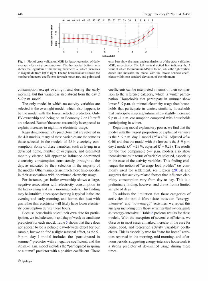
Lasso regression is performed on all survey andactivity data to select influential variables in models ofdaily average electricity consumption and de-minnedaverage electricity consumption. The penalty parameterλ is tuned using 10-fold cross-validation. Figure 4shows the cross-validation procedure. The model withthe minimum MSE (left dotted line) is found with a λvalue of 0.03, includes 23 predictors, and has anMSE of

Fig. 3 Frequency of Benergy-intensive^ activities reported bytime period and time-use category(N = 2218)


0.25. The model with an MSE within one standard errorof the minimum (right dotted line) is found with a λvalue of 0.08 and includes 13 predictors.

First, we include these selected 13 predictors in anOLS regression. Second, we re-run lasso on the fulldata, this time using de-minned average daily elec-tricity consumption as the dependent variable. For thesecond model, lasso selects two new variables andsets two from the first model to zero, meaning thetotal number of selected predictors remains at 13. Weagain include these variables in a simple OLS regres-sion. Table 4 presents regression results, includingunstandardized coefficients (B) and 95% confidenceintervals along with standardized coefficients (β) forboth full-day models, with coefficients listed in orderof standardized coefficient magnitude. For all regres-sion models, we examine diagnostic plots of fittedvalues versus residuals and Q-Q plots. With fewexceptions, these plots confirm normality and linear-ity of the residuals.

Model 1 in Table 4 explains R2 = 49% (adjusted R2 =0.44) of the variance in average electricity consumption,F(13, 159) = 10, p < 0.001. The strongest predictors ofincreased daily consumption are mostly dwelling andappliance-related variables, especially EV ownership,number of power showers, living in a detached home,number of rooms, and number of TVs/computers.Socio-demographic variables that correlate to increasedusage include cat ownership and number of occupants.The only activity category variable selected is recrea-tion; number of recreation activities reported is associ-ated with increased daily average consumption.

Ownership of a gas boiler and being on a renewableor Bgreen^ electricity tariff are the only variables in themodel that predict decreases in average daily consump-tion. The former effect is likely observed because notowning a gas boiler indicates higher use of electricity forspace and water heating. The latter effect may reflect apredisposition to conserve electricity among those whoopt in to a renewable tariff.

The second model in Table 4, for which the depen-dent variable is de-minned average daily electricity con-sumption, explains R2 = 43% (adjusted R2 = 0.38) of thevariance of the dependent variable, F(13, 159) = 9.2,p < 0.001. In addition to the variables in model 1, lassoselects being on an Economy 7 or 10 tariff, whichtypically charge lower prices for nighttime or Boff-peak^electricity use, and number of night storage heaters.Both have positive coefficients but high uncertainty.

This model drops EVownership and number of roomsas predictors.

In general, the differences between models 1 and 2are slight, with model 2 showing slightly lower explan-atory power than model 1. Notably, we do not findadditional activity variables are selected in model 2,even though we might suspect activities to show astronger association to de-minned rather than averagedaily consumption. We return to this finding in theBDiscussion^ section.

To further investigate how categories of time-useactivities might explain patterns in household electricityconsumption, we model de-minned average electricityuse over 4-h time periods. Lasso regression is used toselect models (which can have varying numbers ofpredictors), and we again include lasso-selected vari-ables in an OLS regression for each 4-h period to inves-tigate model coefficients. Table 5 shows variables andunstandardized coefficients with 95% confidence inter-vals. We exclude standardized coefficients from thistable for simplicity but include these in a table in theAppendix.

Table 5 shows that for all times of day except 1 a.m.–5 a.m., activity category variables are frequently select-ed in these models and show strong associations to de-minned electricity consumption. Activities in the Bcarefor home,^ Bfood,^ and Brecreation^ categories, in par-ticular, are consistently selected as influential predictorsacross 4-h models.

Coefficients for activity variables show how differenttypes of activities vary in their associations to electricityconsumption at different times of day. Care for thehome, which includes some energy-intensive householdchores, has a stronger association with de-minned con-sumption in the early evening, mid-morning, and after-noon models and a weaker association in the late eve-ning and early morning models. It is absent from theovernight model (1–5 a.m.) as well as from the day 2 5–9 p.m. model. Food-related activities follow patterns oftypical mealtimes, with stronger coefficients in the eve-nings, early morning, and afternoon. The models do notshow a consistent result in terms of the influence ofdifferent mealtimes on consumption, as the food coeffi-cient for the morning mealtime is larger than in the day 15–9 p.m. model but smaller than in the day 2 5–9 p.m.model. This finding highlights that electricity consump-tion of food preparation and consumption can varybetween days during the same mealtimes. Recreationactivities show strong associations to electricity


consumption except overnight and during the earlymorning, but this variable is also absent from the day 25–9 p.m. model.

The only model in which no activity variables areselected is the overnight model, which also happens tobe the model with the fewest selected predictors. OnlyEVownership and being on an Economy 7 or 10 tariffare selected. Both of these can reasonably be expected toexplain increases in nighttime electricity usage.

Regarding non-activity predictors that are selected inthe 4-h models, many of these variables are the same asthose selected in the models of 28-h electricity con-sumption. Some of these variables, such as living in adetached home, number of occupants, and estimatedmonthly electric bill appear to influence de-minnedelectricity consumption consistently throughout theday, as indicated by their selection in the majority ofthe models. Other variables are muchmore time-specificin their associations with de-minned electricity usage.

For instance, gas boiler ownership shows a large,negative association with electricity consumption inthe late evening and early morning models. This findingmay be intuitive, since space heating is typical in the lateevening and early morning, and homes that heat withgas rather than electricity will likely have lower electric-ity consumption during these hours.

Because households select their own date for partic-ipation, we include season and day of week as candidatepredictors for each model. Table 5 shows that there doesnot appear to be a notable day-of-week effect for oursample, but we do find a slight seasonal effect, as the 5–9 p.m. day 1 model includes the Bparticipated insummer^ predictor with a negative coefficient, and the9 p.m.–1 a.m. model includes the Bparticipated in springor autumn^ predictor with a positive coefficient. These

coefficients can be interpreted in terms of their compar-ison to the reference category, which is winter partici-pation. Households that participate in summer showlower 5–9 p.m. de-minned electricity usage than house-holds that participate in winter; similarly, householdsthat participate in spring/autumn show slightly increased9 p.m.–1 a.m. consumption compared with householdsparticipating in winter.

Regarding model explanatory power, we find that themodel with the largest proportion of explained varianceis the 5–9 p.m. day 1 model (R2 = 43%, adjusted R2 =0.40) and that the model with the lowest is the 5–9 p.m.day 2 model (R2 = 25%, adjustedR2 = 0.23). The resultsfor the two comparable 5–9 p.m. models also showinconsistencies in terms of variables selected, especiallyin the case of the activity variables. This finding chal-lenges the notion of Baverage load profiles^ (as com-monly used for settlement, see Elexon (2013)) andsuggests that activity-related factors that influence elec-tricity consumption vary from day to day. This is apreliminary finding, however, and draws from a limitedsample of days.

To address the limitation that these categories ofactivities do not differentiate between Benergy-intensive^ and Blow-energy^ activities, we repeat thisanalysis including only those activities that we designateas Benergy-intensive.^ Table 6 presents results for thesemodels. With the exception of several coefficients, weobserve in most cases a marked increase in the care forhome, food, and recreation activity variables’ coeffi-cients. This is especially true for Bcare for home^ activ-ities reported in the morning, mid-morning, and after-noon periods, suggesting energy-intensive housework isa strong predictor of de-minned usage during thesetimes.

Fig. 4 Plot of cross-validation MSE for lasso regression of dailyaverage electricity consumption. The horizontal bottom axisshows the logarithm of the tuning parameter λ, which increasesin magnitude from left to right. The top horizontal axis shows thenumber of nonzero coefficients for each model run, and points and

error bars show themean and standard error of the cross-validationMSE, respectively. The left vertical dotted line indicates the λvalue at which the minimumMSE is found, while the right verticaldotted line indicates the model with the fewest nonzero coeffi-cients within one standard deviation of the minimum


In some instances, the energy-intensive activitymodels either drop or add activity-related variables fordifferent times of day. While the Bcare for home^ cate-gory when not filtering for energy-intensive activities isselected in the day 1 5–9 p.m. and the 9 p.m.–1 a.m.models, it is not selected when only energy-intensiveactivities are included. This may suggest that moreenergy-intensive activities related to household choresare not as common in the evenings. It also indicates thatBcare for home^ as a category includes non-energy-intensive activities that are important for explainingelectricity consumption during evenings.

Similar distinctions are found for food-related activ-ities. The model including only energy-intensive foodactivities more clearly differentiates between eveningand morning meals, as morning food activities showless associations with electricity consumption when ex-cluding non-energy-intensive activities, likely becausemorning meals are often cold and do not involve appli-ance use. For recreation activities, the timing of whenthese are influential does not change between the two

different categorizations, though the strength of associ-ations clearly increases when only energy-intensive ac-tivities are included.

To test the extent to which categorized activity dataimproves model explanatory power, we compute theadjusted R2 value for each model excluding the lasso-selected activity predictors for that model, and we dothis for both categorizations tested.2 We present theseresults in Table 7. We see that excluding activity datareduces model explanatory power by an average of ninepercentage points acrossmodels (excluding the 1–5 a.m.model). We do not observe, however, a noticeable dif-ference between the models including all activity dataand those including only Benergy-intensive^ activities.These findings provide evidence of the potential im-provements to household electricity modeling by in-cluding activity data, even when it is relatively coarselycategorized.

Table 4 Regression results for average electricity usage and average de-minned usage during full 28-h study period

1) Daily average (W) 2) De-minned daily average (W)

B (5–95% CI) β B (5–95% CI) β

EV 0.61** (0.18, 1.04) 0.61

Tariff: Renewable − 0.30** (− 0.50, − 0.11) − 0.30 − 0.30* (− 0.54, − 0.06) − 0.26

Gas boiler − 0.27* (− 0.48, − 0.06) − 0.27 − 0.19 (− 0.46, 0.09) − 0.16

Owns cat 0.25** (0.08, 0.43) 0.25 0.18 (− 0.04, 0.39) 0.24

Tariff: Economy 7 or 10 0.43 (− 0.03, 0.88) 0.24

Recreation activities 0.02** (0.01, 0.03) 0.24 0.03*** (0.01, 0.04) 0.23

No. of power showers 0.15* (0.03, 0.27) 0.19 0.13 (− 0.02, 0.28) 0.18

Detached home 0.19 (− 0.04, 0.43) 0.19 0.45** (0.18, 0.73) 0.34

No. of rooms 0.07* (0.005, 0.14) 0.18

No. of TV/computers 0.06* (0.004, 0.12) 0.17 0.06 (− 0.02, 0.13) 0.18

Under floor heating 0.16 (− 0.03, 0.35) 0.16 0.16 (− 0.07, 0.40) 0.20

Tumble dryer 0.10 (− 0.07, 0.27) 0.10 0.10 (− 0.11, 0.30) 0.08

No. of night storage heaters 0.07 (− 0.11, 0.25) 0.01

Estimated monthly electric bill 0.03 (− 0.02, 0.09) 0.10 0.02 (− 0.05, 0.09) 0.13

No. of occupants 0.03 (− 0.04, 0.10) 0.08 0.08 (− 0.01, 0.16) 0.11

Constant 5.42*** (5.10, 5.74) 6.27 4.97*** (4.61, 5.33) 6.15

Observations 173 173

R2 0.49 0.43

Adjusted R2 0.44 0.38

Residual std. error (df = 159) 0.47 0.57

*p < 0.05; **p < 0.01; ***p < 0.001

2 Adjusted R2 is used for the comparison in order to account for thevarying number of predictors in each model.


Table 5 Regression results for de-minned average electricity use: 4-h models (5 p.m. day 1–9 p.m. day 2)

Predictor 5–9 p.m. (1) 5–9 p.m. (2) 9 p.m.–1 a.m. 1 a.m.–5a.m.

5 a.m.–9 a.m. 9 a.m.–1p.m.

1 p.m.–5p.m.

Activity categories

Care for home 0.17***(0.09, 0.24)

0.16*(0.002, 0.32)

0.16(− 0.07, 0.39)

0.15(− 0.02,

0.33)

0.15(− 0.03,

0.32)

Care for others 0.15(− 0.04, 0.33)

0.35**(0.10, 0.60)

Food 0.03(− 0.02, 0.07)

0.10***(0.05, 0.15)

0.08*(0.01, 0.16)

0.06(− 0.01, 0.13)

0.08(− 0.02,

0.19)

Other activity 0.22*(0.02, 0.43)

Recreation 0.06*(0.01, 0.12)

0.08*(0.01, 0.15)

0.21*(0.02, 0.39)

0.25*(0.04, 0.46)

Appliances

EV 2.23***(1.06, 3.40)

Gas boiler − 0.37*(− 0.65,

− 0.09)

− 0.59**(− 0.99,

− 0.20)Heat pump 0.76

(− 0.20, 1.72)No. of night storage heaters 0.39**

(0.15, 0.63)

No. of power showers 0.23**(0.06, 0.39)

0.27*(0.01, 0.53)

No. of TVs/computers 0.07(− 0.04,

0.18)

0.17**(0.04, 0.30)

0.09(− 0.04,

0.22)

Tumble dryer 0.28(− 0.04, 0.60)

0.37*(0.01, 0.74)

Under floor heating 0.11(− 0.15, 0.37)

0.34(− 0.04, 0.72)

Dwelling

Detached home 0.62***(0.29, 0.95)

0.56**(0.15, 0.97)

0.20(− 0.10, 0.50)

0.17(− 0.25, 0.59)

0.66**(0.19, 1.14)

No. of rooms in home 0.08(− 0.05,

0.20)

0.10(− 0.04,

0.23)

0.08(− 0.06,

0.22)

Terraced home − 0.16(− 0.41, 0.08)

Socio-demographics

Bill affordability − 0.18*(− 0.35,

− 0.01)Estimated monthly electricbill

0.09(− 0.01,

0.19)

0.06(− 0.02, 0.13)

0.09(− 0.02, 0.19)

0.08(− 0.04,

0.21)No. of occupants 0.13*

(0.03, 0.22)0.06(− 0.03, 0.15)

0.09(− 0.06, 0.23)

0.13


Discussion

Summary and discussion of results

The results show that 13 lasso-selected predictors canexplain 49% of full-day average household electricityusage. When the dependent variable is Bde-minned^ toremove baseload consumption, lasso selects a model thatexplains 43% of the variance in average de-minned elec-tricity usage. These results are consistent with or in somecases improve on model explanatory power found inprevious studies of household electricity usage (Huebneret al. 2016; Kavousian et al. 2013; McLoughlin et al.2012). For themodels of 4-h average de-minned electricityconsumption, explanatory power is somewhat lower, rang-ing from 25 to 43% of variance explained. These modelsinclude varying numbers of lasso-selected predictors, butwe find that removing activity variables from these modelsreduces their explanatory power considerably.

The results for both full-daymodels confirm previousfindings that appliance ownership and occupant socio-demographics show the strongest associations to elec-tricity consumption patterns (Huebner et al. 2016).

These results also, however, identify new variables thatmight help predict daily usage, such as electricity tariffchoice or pet ownership. The results provide some evi-dence that these may be important for understandingelectricity consumption patterns.

This study goes beyond previous research by investi-gating how the associations between appliance, dwelling,and socio-demographic variables and de-minned electric-ity consumption vary as a function of time of day. The EVownership variable, for instance, is only selected in thenighttime model, which suggests that ownership of anEV increases a household’s nighttime consumption moreso than it increases consumption during other times.Similarly, the number of power showers and presenceof underfloor heating are associated with consumptionduring late evening and morning hours, when showersare likely more frequent. Number of TVs/computersowned is a stronger predictor in themorning and evening.

The study also tests the extent to which differenttypes of activities are associated with electricity con-sumption during different periods of the day. We findevidence that certain types of activities are more relevantfor understanding electricity consumption patterns and

Table 5 (continued)

Predictor 5–9 p.m. (1) 5–9 p.m. (2) 9 p.m.–1 a.m. 1 a.m.–5a.m.

5 a.m.–9 a.m. 9 a.m.–1p.m.

1 p.m.–5p.m.

(− 0.02,0.27)

Owns cat 0.31(− 0.01,

0.64)

0.36**(0.12, 0.59)

0.35*(0.02, 0.69)

Participated in summer − 0.43***(− 0.67,

− 0.18)Participated inspring/autumn

0.34**(0.09, 0.59)

Tariff: Economy 7 or 10 1.73***(1.07, 2.40)

Tariff: Renewable − 0.42**(− 0.72,

− 0.11)

− 0.43**(− 0.69,

− 0.17)Tenure (rent vs. own) − 0.38*

(− 0.73,− 0.02)

Constant 5.82***(5.38, 6.26)

4.55***(4.00, 5.10)

5.04***(4.68, 5.40)

3.92***(3.75, 4.09)

4.53***(3.98, 5.07)

3.53***(2.91, 4.15)

3.42***(2.79, 4.04)

Observations 171 170 172 172 172 170 170

R2 0.43 0.25 0.43 0.28 0.33 0.29 0.39

Adjusted R2 0.40 0.23 0.39 0.27 0.28 0.26 0.35

*p < 0.05; **p < 0.01; ***p < 0.001


Tab

le6

Regressionresults

forde-m

innedaverageelectricity

use:4-hmodels(5

p.m.day

1–9p.m.day

2)includingonly

Benergy-intensive^

activ

ities

across

categories

Predictor

5–9p.m.(1)

5–9p.m.(2)

9p.m.–1a.m.

1a.m.–5a.m.

5a.m.–9a.m.

9a.m.–1p.m.

1p.m.–5p.m.

Activity

categories

Careforhome

1.05**

(0.39,1.71)

0.52*

(0.13,0.91)

0.70**

(0.24,1.15)

Careforself

0.11

(−0.05,0.27)

Food

0.02

(−0.06,0.11)

0.18**

(0.06,0.30)

0.23**

(0.06,0.40)

0.14

(−0.07,0.35)

0.20*

(0.01,0.39)

Recreation

0.10**

(0.04,0.16)

0.20***

(0.10,0.29)

0.35**

(0.12,0.58)

0.30*

(0.05,0.55)

Appliances

EV

2.23***

(1.06,3.40)

Gas

boiler

−0.32*

(−0.59,−

0.05)

−0.65***

(−1.03,−

0.27)

No.of

nightstorage

heaters

0.42***

(0.18,0.66)

No.of

power

show

ers

0.26**

(0.10,0.42)

0.22

(−0.05,0.49)

No.of

TVs/computers

0.14*

(0.01,0.27)

0.08

(−0.05,0.20)

Tum

bledryer

0.34

(−0.03,0.71)

0.38*

(0.02,0.75)

Under

floorheating

0.12

(−0.13,0.38)

0.40*

(0.03,0.77)

0.38

(−0.05,0.81)

Dwellin

g

Detachedhome

0.68***

(0.34,1.03)

0.66**

(0.24,1.07)

0.20

(−0.09,0.50)

0.28

(−0.14,0.69)

0.18

(−0.32,0.69)

0.76**

(0.28,1.24)

No.of

room

sin

home

0.08

(−0.04,0.21)

−0.01

(−0.16,0.14)

0.07

(−0.07,0.21)

Terraced

home

−0.13

(−0.39,0.13)

Socio-demographics

Estim

ated

monthly

electricbill

0.11*

(0.01,0.21)

0.04

(−0.03,0.11)

0.10

(−0.01,0.20)

0.04

(−0.08,0.17)

No.of

occupants

0.16**

(0.06,0.26)

0.08

(−0.01,0.17)

0.15*

(0.01,0.29)

0.12

(−0.04,0.28)

0.15*

(0.001,0.30)

Owns

cat

0.33**

(0.10,0.56)

0.33

(−0.01,0.67)

−0.43**


also that certain activities have stronger or weaker asso-ciations at different times of day.

Inparticular,our results showthathousework,eatingandmeal preparation, and recreation or media use are stronglyassociated with de-minned electricity consumption,confirming similar findings from previous research(Anderson and Torriti 2018; De Lauretis et al. 2017; Jalasand Juntunen 2015; Palmer et al. 2013). The times atwhichthese activities are stronger predictors of electricity con-sumption also provides insight into when activities andelectricity use are more tightly coupled, such as duringevening peak periods and later evenings for food and recre-ational activities, earlymornings for personal care activities,and early andmid-mornings for household chores.

Our results also highlight the extent to whichdenoting activities as Benergy-intensive^ can strengthenthese links. We find in general a sizeable increase in thestrength of relationships between number of activitiesreported and average de-minned electricity consumptionthroughout the day when including only Benergy-intensive^ activities. We do note, however, that theseresults are somewhat mixed. For instance, the Bcare forhome^ variable is significant in the day 1 5–9 p.m.model when including all activity data but not whenincluding only energy-intensive activities. This findingsuggests other Bcare for home^ activities are importantfor explaining electricity consumption during this time.While acknowledging that our designation of activitiesas Benergy-intensive^ is subjective, we take this findingas evidence that the links between activities and elec-tricity consumption may be more complex than simplydifferentiating activities on the basis of their expecteduse of energy. Further discussion of this point can befound in Grünewald and Diakonova (2018b).

Two additional results merit further discussion. Thefirst is our finding that we do not observe an increase inthe number of activity variables selected between thedaily average and daily de-minned average models. Wedo, however, observe frequent selection of activity var-iables in the 4-h de-minned usage models. We expectthat this observation results from the duration of timeover which we are de-minning electricity consumption.Over a 28-h period, de-minning does not appear to yieldstronger associations between activities reported andaverage consumption. Over shorter 4-h periods, howev-er, de-minning does appear to strengthen relationshipsbetween reported activities and consumption. This find-ing suggests that activity data can improve models ofshorter duration more so than it can models of longerT

able6

(contin

ued)

Predictor

5–9p.m.(1)

5–9p.m.(2)

9p.m.–1a.m.

1a.m.–5a.m.

5a.m.–9a.m.

9a.m.–1p.m.

1p.m.–5p.m.

Participated

insummer

(−0.69,−

0.17)

Participated

inspring/autum

n0.36**

(0.12,0.61)

Participated

onFri–Sat

0.56*

(0.11,1.01)

Tariff:E

conomy

7or

101.73***

(1.07,2.40)

Tariff:R

enew

able

−0.51**

(−0.81,−

0.20)

−0.40**

(−0.65,−

0.14)

Constant

5.56***

(5.24,5.87)

4.77***

(4.24,5.31)

4.99***

(4.63,5.34)

3.92***

(3.75,4.09)

4.52***

(4.03,5.00)

3.62***

(2.97,4.28)

3.48***

(2.86,4.11)

Observations

171

170

172

172

172

170

170

R2

0.35

0.20

0.45

0.28

0.30

0.33

0.37

AdjustedR2

0.32

0.18

0.41

0.27

0.26

0.28

0.34

*p<0.05;*

*p<0.01;*

**p<0.001


duration. We expect activities to show increasinglystrong associations to more finely resolved electricityreadings, and this is something we are exploring incurrent research.

The second result deserving of further discussion is ourfinding that the models for the day 1 5–9 p.m. period andthe day 2 5–9 p.m. period show considerable differencesin the variables selected and in model explanatory power.We note that fewer activities are reported during the day 25–9 p.m. period, but given that lasso standardizes predic-tors prior to selection, this should not influence the algo-rithm’s selection procedure. Furthermore, we note that the1–5 p.m. model includes several activity variables and agreater explanatory power than the day 2 5–9 p.m. model,even with far fewer activities reported. We take this resultto suggest that the relationship between activities andelectricity consumption may vary considerably in thesame households between days and also that peak hoursmay be especially variable. This finding, too, warrantsfurther exploration in future research.

Policy implications

These results have implications both for energy demandmodels and for policy considerations surrounding de-mand flexibility and DSR. First, we have shown thatactivity data, whether categorized as Benergy-intensive^or not, can improve models of household electricity use.For at least one of our Bpeak period^ models, we findthat activity data is especially useful for understandingvariations in de-minned electricity use during thesehours.

Our novel approach to collect time-use data in paral-lel with electricity consumption can overcome many ofthe limitations and challenges previously discussed inthe literature on time-use or activity-based models ofenergy demand (McKenna et al. 2017; Torriti 2014).Specifically, this method enables the collection of moreenergy-relevant activities, which we have shown toincrease the strength and statistical validity of the rela-tionships between household activities and electricityconsumption. Given the lack of empirical evidence onthese relationships, these results can help improve thespecification of activity-appliance signals in modelsincorporating time-use data. Our approach also facili-tates the collection of activity data from multi-occupanthouseholds, which have previously been more difficultto account for in time-use models of electricity demand.

Second, while some literature has concluded that it issufficient to model active occupancy states for the purposeof constructing more accurate energy demand models, webelieve that such an approach fails tomore directly link thetypes of activities that are being performed during Bactiveoccupancy,^which have important consequences and pol-icy implications for delivering more flexible demand.

Our results show that certain types of activities havestronger relationships to electricity consumption at dif-ferent times of day. Targeting these activities in DSRinterventions could yield larger shifts in demand. Fur-thermore, tailoring DSR interventions based on betterevidence about what is actually occurring in householdsduring peak times and about how these activities varyamong different segments of the population can im-prove their effectiveness while also mitigating theirimpact on vulnerable populations.

Table 7 Model explanatory power with and without lasso-selected activity variables for both Ball^ activity data and Benergy-intensive^activity data models

5–9 p.m.(1)

5–9 p.m.(2)

9 p.m.–1a.m.

1 a.m.–5 a.m.

5 a.m.–9 a.m.

9 a.m.–1p.m.

1 p.m.–5p.m.

BAll^ activity models

Adjusted R2 0.40 0.23 0.39 0.27 0.28 0.26 0.35

Adjusted R2 withoutactivity variables

0.28 0.17 0.30 – 0.25 0.13 0.23

Difference in adj R2 0.12 0.06 0.09 – 0.03 0.13 0.12

BEnergy-intensive^ activity models

Adjusted R2 0.31 0.18 0.41 0.27 0.26 0.28 0.34

Adjusted R2 withoutactivity variables

0.27 0.15 0.30 – 0.22 0.18 0.23

Difference in adj R2 0.04 0.03 0.11 – 0.04 0.10 0.11


In terms of potential for shifting demand alone, theseresults suggest food preparation and meal times, house-hold chores, and recreational activities should be prior-itized for activity-led DSR given their strong associa-tions with electricity use. But this is not the only con-sideration upon which effective DSR strategies shouldbe based. Other considerations, such as those compris-ing Torriti et al.’s (2015) BFlexibility Index^, are alsovaluable for determining which activities at which timescan be shifted without adverse social impacts.

Study limitations

Some limitations are present in this analysis. The sampleis non-representative, and several sample biases are pres-ent. The sample size is also small relative to the numberof predictors. Standard errors for most variables in theregression models are therefore large in comparison tocoefficient size. Models are not constructed for differentdays of week or seasons in order to preserve the samplesize, but these variables are instead included at the modelselection stage. Furthermore, self-reported activities canlead to biases and inaccuracies. Measuring activities assimple frequency counts is a coarse way to include thesedata and may obfuscate more complex relationshipsbetween activity type, timing, and electricityconsumption. A similar approach as the one taken byRhodes et al. (2014) and McLoughlin et al. (2015), whocluster load profiles and use household characteristics tobuild predictive models of membership in distinctiveload profiles, may be instructive in this context. Time-use data may be even better suited to this approach thansocio-demographic, dwelling, or appliance ownershipdata, due to its temporal resolution.

Our initial categorization of activity data relies on ataxonomy that was not developed for energy modelingpurposes, and although we make an attempt at catego-rizing activities as Benergy-intensive,^ this is a subjec-tive exercise. We believe much more work could bedone to identify more energy-relevant activity catego-ries with useful implications for energy demand model-ing and for estimating the potential of demand response(Anderson 2016).

Finally, more data from a more representative sampleof households could reduce uncertainty surrounding thestrength of relationships between predictive variables andelectricity consumption and could make these resultsmore generalizable. The data collection is ongoing, suchthat more detailed analyses can be conducted in future.

We believe there is potential to scale this research tomuchlarger (> 1000 households), nationally representativesamples using app-based activity diaries coupled withsmart meter data, and preparations are underway forscaling this study. We also encourage similar studiesacross varying cultural and societal contexts.

Conclusions

This paper presents analysis of intra-day electricity con-sumption for a sample of 173 UK households. Electric-ity provision during peak times is costly and challengingin energy systems with high penetrations of renewableelectricity. Understanding the drivers behind electricityconsumption during peak times can assist in the designof more effective intervention strategies to shift electric-ity use patterns in the residential sector.

We present regressionmodels of average full-day and4-h de-minned electricity consumption using a widerange of predictive factors, including socio-demograph-ic, physical dwelling, appliance ownership, and catego-rized activity variables. Our analysis tests the ability ofthese variables to explain consumption at different timesof day and the strength of these relationships.

Our results show that adding activity data to regres-sion models can improve their explanatory power of de-minned electricity consumption during most times ofday. This result holds regardless of whether only activ-ities that we reasonably assume to be Benergy-intensive^are included. Given how challenging it is to achievegreater explanatory power of highly diverse electricityuses in households, a nine-percentage point increase inadjusted R2 on average is encouraging. The results alsoshow strong associations between activities and electric-ity consumption at different times of day. The impor-tance of household chores, food, and recreation activi-ties for explaining electricity consumption patterns isclearly demonstrated.

We expect that more nuanced categorizations of ac-tivities and investigations of their relationship to elec-tricity consumption at more finely resolved timescaleswill yield improved insights into the flexibility of de-mand. This evidence could reduce the cost of integratingrenewable energy sources into existing energy systemsby providing a better estimate of the potential ofdemand-side response in the residential sector, thuscontributing to accelerating the low-carbon energytransition.


Funding information This research received funding from theEngineering and Physical Sciences Research Council (EPSRC)under grant EP/M024652/1.Data availabilityThe data that supportthe findings of this study are available from the correspondingauthor upon request. The tools used for time-use and electricitydata collection are publicly available at https://goo.gl/81mvCB.

Compliance with ethical standards The University of Ox-ford’s Central University Research Ethics Committee (CUREC)has approved this study.

Conflict of interest The authors declare that they have no con-flicts of interest.

Appendix

Table 8 Standardized regression coefficients for Table 5

5–9 p.m. (1) 5–9 p.m. (2) 9 p.m.–1 a.m. 1 a.m.–5 a.m. 5 a.m.–9 a.m. 9 a.m.–1 p.m. 1 p.m.–5 p.m.Predictor β β β β β β β

Activity categories

Care for home 0.46*** 0.21* 0.22 0.32 0.28

Care for others 0.23 0.49**

Food 0.16 0.52*** 0.25* 0.25 0.31

Other activity 0.37*

Recreation 0.33* 0.25* 0.42* 0.44*

Appliances

EV 2.23***

Gas boiler − 0.37* − 0.59**Heat pump 0.76

No. of night storage heaters 0.53**

No. of power showers 0.29** 0.35*

No. of TVs/computers 0.19*** 0.46** 0.24

Tumble dryer 0.28 0.37*

Under floor heating 0.11 0.34

Dwelling

Detached home 0.62*** 0.56** 0.20 0.17 0.66**

No. of rooms in home 0.20** 0.25 0.21

Terraced home − 0.16Socio-demographics

Bill affordability − 0.24*Estimated monthly electric bill 0.27*** 0.18 0.26 0.25

No. of occupants 0.30* 0.14 0.20 0.29

Owns cat 0.31 0.36** 0.35*

Participated in summer − 0.43***Participated in spring/autumn 0.34**

Tariff: Economy 7 or 10 1.73***

Tariff: Renewable − 0.42** − 0.43**Tenure (rent vs. own) − 0.38*Constant 6.19 5.66 5.66 4.10 5.28 4.99 4.75

Observations 171 170 172 172 172 170 170

R2 0.43 0.25 0.43 0.28 0.33 0.29 0.39

Adjusted R2 0.40 0.23 0.39 0.27 0.28 0.26 0.35

*p < 0.05; **p < 0.01; ***p < 0.001


https://goo.gl/81mvCB

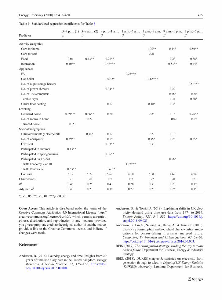
Open Access This article is distributed under the terms of theCreative Commons Attribution 4.0 International License (http://creativecommons.org/licenses/by/4.0/), which permits unrestrict-ed use, distribution, and reproduction in any medium, providedyou give appropriate credit to the original author(s) and the source,provide a link to the Creative Commons license, and indicate ifchanges were made.

References

Anderson, B. (2016). Laundry, energy and time: Insights from 20years of time-use diary data in the United Kingdom. EnergyResearch & Social Science, 22, 125–136. https://doi.org/10.1016/j.erss.2016.09.004.

Anderson, B., & Torriti, J. (2018). Explaining shifts in UK elec-tricity demand using time use data from 1974 to 2014.Energy Policy, 123, 544–557. https://doi.org/10.1016/j.enpol.2018.09.025.

Anderson, B., Lin, S., Newing, A., Bahaj, A., & James, P. (2016).Electricity consumption and household characteristics: impli-cations for census-taking in a smart metered future.Computers, Environment and Urban Systems, 63, 58–67.https://doi.org/10.1016/j.compenvurbsys.2016.06.003.

BEIS. (2017). The clean growth strategy: leading the way to a lowcarbon future. Department for Business, Energy & IndustrialStrategy.

BEIS. (2018). DUKES chapter 5: statistics on electricity fromgeneration through to sales. In Digest of UK Energy Statistics(DUKES): electricity. London: Department for Business,

Table 9 Standardized regression coefficients for Table 6

5–9 p.m. (1) 5–9 p.m. (2) 9 p.m.–1 a.m. 1 a.m.–5 a.m. 5 a.m.–9 a.m. 9 a.m.–1 p.m. 1 p.m.–5 p.m.Predictor β β β β β β β

Activity categories

Care for home 1.05** 0.44* 0.50**

Care for self 0.21

Food 0.04 0.43** 0.28** 0.23 0.38*

Recreation 0.40** 0.43*** 0.53** 0.44*

Appliances

EV 2.23***

Gas boiler − 0.32* − 0.65***No. of night storage heaters 0.56***

No. of power showers 0.34** 0.29

No. of TVs/computers 0.38* 0.20

Tumble dryer 0.34 0.38*

Under floor heating 0.12 0.40* 0.38

Dwelling

Detached home 0.69*** 0.66** 0.20 0.28 0.18 0.76**

No. of rooms in home 0.22 − 0.02 0.19

Terraced home − 0.15Socio-demographics

Estimated monthly electric bill 0.34* 0.12 0.29 0.13

No. of occupants 0.39** 0.19 0.35* 0.28 0.35*

Owns cat 0.33** 0.33

Participated in summer − 0.43**Participated in spring/autumn 0.36**

Participated on Fri–Sat 0.56*

Tariff: Economy 7 or 10 1.73***

Tariff: Renewable − 0.53** − 0.40**Constant 6.19 5.72 5.62 4.10 5.34 4.69 4.74

Observations 171 170 172 172 172 170 170

R2 0.43 0.25 0.43 0.28 0.33 0.29 0.39

Adjusted R2 0.40 0.23 0.39 0.27 0.28 0.26 0.35

*p < 0.05; **p < 0.01; ***p < 0.001


https://doi.org/10.1016/j.erss.2016.09.004


https://doi.org/10.1016/j.enpol.2018.09.025


https://doi.org/10.1016/j.compenvurbsys.2016.06.003

Energy & Industr ial Strategy https: / /www.gov.uk/government/statistics/electricity-chapter-5-digest-of-united-kingdom-energy-statistics-dukes. Accessed 11 April 2019

CCC. (2016). Annex 2: heat in UK buildings today. In Next stepsfor UK heat policy. London: Committee on Climate Changehttps://www.theccc.org.uk/wp-content/uploads/2017/01/Annex-2-Heat-in-UK-Buildings-Today-Committee-on-Climate-Change-October-2016.pdf . Accessed 12 February2019.

De Lauretis, S., Ghersi, F., & Cayla, J.-M. (2017). Energy consump-tion and activity patterns: an analysis extended to total time andenergy use for French households. Applied Energy, 206, 634–648. https://doi.org/10.1016/j.apenergy.2017.08.180.

DECC. (2012). Demand side response in the domestic sector - aliterature review of major trials. London: Department ofEnergy and Cl imate Change ht tps : / /www.gov.uk/government/uploads/system/uploads/attachment_data/file/48552/5756-demand-side-response-in-the-domestic-sector-a-lit.pdf. Accessed 11 April 2019.

DECC. (2013). Report 9: Domestic appliances, cooking& coolingequipment (No. BRE report number 288143). London:Department of Energy and Climate Change https://www.gov.uk/government/uploads/system/uploads/attachment_data/file/274778/9_Domestic_appliances__cooking_and_cooling_equipment.pdf. Accessed 16 March 2018.

DECC. (2014). Seasonal variations in electricity demand.London: Department of Energy and Climate Changeh t t p s : / / a s s e t s . p u b l i s h i n g . s e r v i c e . g o v .uk/government/uploads/system/uploads/attachment_data/file/295225/Seasonal_variations_in_electricity_demand.pdf . Accessed 12 February 2019.

Druckman, A., Buck, I., Hayward, B., & Jackson, T. (2012). Time,gender and carbon: a study of the carbon implications ofBritish adults’ use of time. Ecological Economics, 84, 153–163. https://doi.org/10.1016/j.ecolecon.2012.09.008.

Elexon. (2013). Load profiles and their use in electricity settlement(p. 31). Elexon www.elexon.co.uk/wp-content/uploads/2013/11/load_profiles_v2.0_cgi.pdf.

Ellegård, K., & Palm, J. (2011). Visualizing energy consumptionactivities as a tool for making everyday life more sustainable.Applied Energy, 88(5), 1920–1926. https://doi.org/10.1016/j.apenergy.2010.11.019.

Ellegård, K., Vrotsou, K., & Widén, J. (2010). VISUAL-TimePAcTS/energy use – a software application for visual-izing energy use from activities performed. In Conferenceproceedings 3rd International Scientific Conference onBEnergy Systems with It^ (pp. 1–17). http://citeseerx.ist.psu.edu/viewdoc/download?doi=10.1.1.468.5526&rep=rep1&type=pdf.

eurostat. (2009). Harmonised European time use surveys: 2008guidelines. Luxembourg: Office for Official Publications ofthe European Communities.

Firth, S., Lomas, K., Wright, A., & Wall, R. (2008). Identifyingtrends in the use of domestic appliances from householdelectricity consumption measurements. Energy andBuildings, 40(5), 926–936. https://doi.org/10.1016/j.enbuild.2007.07.005.

Friedman, J., Hastie, T., & Tibshirani, R. (2010). Regularizationpaths for generalized linear models via coordinate descent.Journal of Statistical Software, 33(1), 1–22.

Gelman, A. (2008). Scaling regression inputs by dividing by twostandard deviations. Statistics in Medicine, 27(15), 2865–2873. https://doi.org/10.1002/sim.3107.

Gelman, A., Su, Y.-S., Yajima, M., Hill, J., Pittau, M. G., Kerman,J., et al. (2018). arm: data analysis using regression andmultilevel/hierarchical models. https://CRAN.R-project.org/package=arm.

Gershuny, J. (2008). Time-use studies: daily life and socialchange: Full Research Report (ESRC End of AwardReport, RES-000-23-0704-A). Swindon: ESRC. https://s3-eu-west-1.amazonaws.com/esrc-files/outputs/DXDg-pyFREKpOk_6bEon8Q/gWE89bsrZEu6BF9Azmg_Cw.pdf

Gershuny, J., & Sullivan, O. (2017). United Kingdom time usesurvey, 2014–2015. [data collection]. UK Data Service. SN:8128. https://doi.org/10.5255/UKDA-SN-8128-1

Grunewald, P., & Diakonova, M. (2018a). Flexibility, dynamismand diversity in energy supply and demand: a critical review.Energy Research & Social Science, 38, 58–66. https://doi.org/10.1016/j.erss.2018.01.014.

Grunewald, P., & Diakonova, M. (2018b). The electricity footprintof household activities - implications for demand models.Energy and Buildings, 174, 635–641. https://doi.org/10.1016/j.enbuild.2018.06.034.

Grünewald, P., & Diakonova, M. (2019). METER data. Energy-use.org. http://www.energy-use.org/docs/data/. Accessed 11April 2019.

Grünewald, P., & Layberry, R. (2015). Measuring the relationshipbetween time-use and electricity consumption. InProceedings of the 2015 ECEEE Summer Study on EnergyEfficiency in Buildings (Vol. 9, pp. 2087–96). Presqu’île deGiens, France: ECEEE. www.eceee.org/library/conference_proceedings/eceee_Summer_Studies/2015/9-dynamics-of-consumption/measuring-the-relationship-between-time-use-and-electricity-consumption/.

Grünewald, P., Diakonova, M., Zilli, D., Bernard, J., & Matousek,A. (2017). What we do matters – a time-use app to captureenergy relevant activities. In Proceedings of the 2017 ECEEESummer Study on Energy Efficiency in Buildings (Vol. 9, pp.2085–93). Presqu’île de Giens, France: ECEEE. www.eceee.org/library/conference_proceedings/eceee_Summer_Studies/2017/9-consumption-and-behaviour/what-we-do-matters-8211-a-time-use-app-to-capture-energy-relevant-activities/.

Harrell, F. (2001). Regression modeling strategies: with applica-tions to linear models, logistic regression, and survival anal-ysis . New York: Springer-Verlag www.springer.com/gb/book/9781441929181.

Hsu, D. (2015). Identifying key variables and interactions instatistical models of building energy consumption using reg-ularization. Energy, 83, 144–155. https://doi.org/10.1016/j.energy.2015.02.008.

Huebner, G., Shipworth, D., Hamilton, I., Chalabi, Z., &Oreszczyn, T. (2016). Understanding electricity consump-tion: a comparative contribution of building factors, socio-demographics, appliances, behaviours and attitudes. AppliedEnergy, 177 , 692–702. https://doi.org/10.1016/j.apenergy.2016.04.075.

Jalas, M., & Juntunen, J. K. (2015). Energy intensive lifestyles:time use, the activity patterns of consumers, and relatedenergy demands in Finland. Ecological Economics, 113,51–59. https://doi.org/10.1016/j.ecolecon.2015.02.016.


https://www.gov.uk/government/statistics/electricity-chapter-5-digest-of-united-kingdom-energy-statistics-dukes



https://www.theccc.org.uk/wp-content/uploads/2017/01/Annex-2-Heat-in-UK-Buildings-Today-Committee-on-Climate-Change-October-2016.pdf



https://doi.org/10.1016/j.apenergy.2017.08.180

https://www.gov.uk/government/uploads/system/uploads/attachment_data/file/48552/5756-demand-side-response-in-the-domestic-sector-a-lit.pdf




https://www.gov.uk/government/uploads/system/uploads/attachment_data/file/274778/9_Domestic_appliances__cooking_and_cooling_equipment.pdf




https://assets.publishing.service.gov.uk/government/uploads/system/uploads/attachment_data/file/295225/Seasonal_variations_in_electricity_demand.pdf




https://doi.org/10.1016/j.ecolecon.2012.09.008

http://www.elexon.co.uk/wp-content/uploads/2013/11/load_profiles_v2.0_cgi.pdf

http://www.elexon.co.uk/wp-content/uploads/2013/11/load_profiles_v2.0_cgi.pdf



http://citeseerx.ist.psu.edu/viewdoc/download?doi=10.1.1.468.5526&rep=rep1&type=pdf



https://doi.org/10.1016/j.enbuild.2007.07.005


https://doi.org/10.1002/sim.3107

https://cran.r-project.org/package=arm

https://cran.r-project.org/package=arm

https://s3-eu-west-1.amazonaws.com/esrc-files/outputs/DXDg-pyFREKpOk_6bEon8Q/gWE89bsrZEu6BF9Azmg_Cw.pdf



https://doi.org/10.5255/UKDA-SN-8128-1





http://energy-use.org

http://energy-use.org

http://www.energy-use.org/docs/data/

http://www.eceee.org/library/conference_proceedings/eceee_Summer_Studies/2015/9-dynamics-of-consumption/measuring-the-relationship-between-time-use-and-electricity-consumption/




http://www.eceee.org/library/conference_proceedings/eceee_Summer_Studies/2017/9-consumption-and-behaviour/what-we-do-matters-8211-a-time-use-app-to-capture-energy-relevant-activities/





http://www.springer.com/gb/book/9781441929181

http://www.springer.com/gb/book/9781441929181

https://doi.org/10.1016/j.energy.2015.02.008




https://doi.org/10.1016/j.ecolecon.2015.02.016

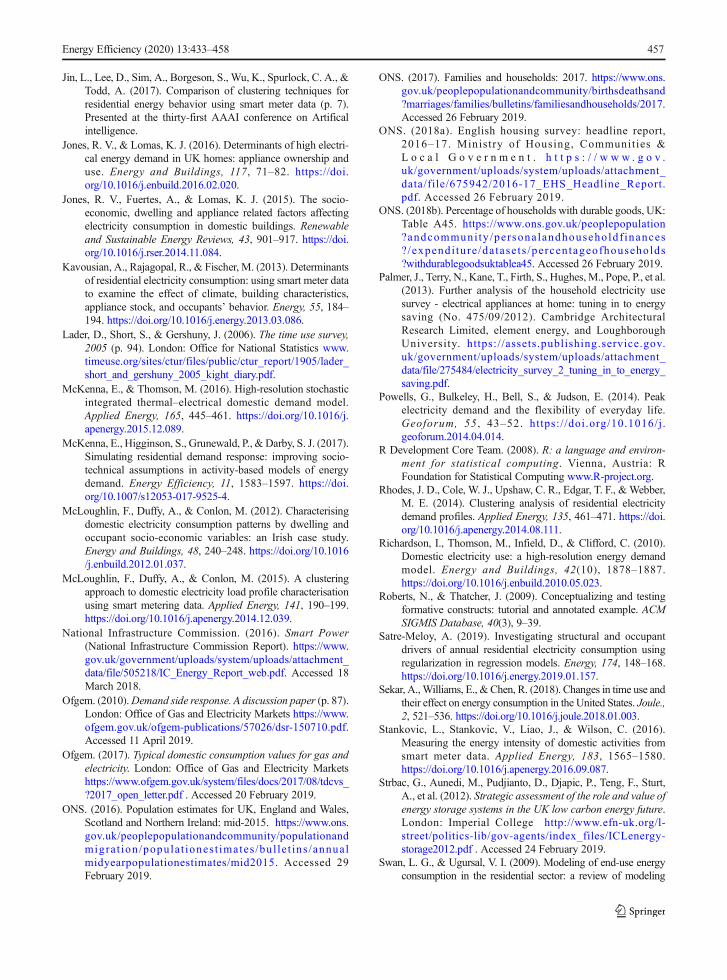
Jin, L., Lee, D., Sim, A., Borgeson, S., Wu, K., Spurlock, C. A., &Todd, A. (2017). Comparison of clustering techniques forresidential energy behavior using smart meter data (p. 7).Presented at the thirty-first AAAI conference on Artificalintelligence.

Jones, R. V., & Lomas, K. J. (2016). Determinants of high electri-cal energy demand in UK homes: appliance ownership anduse. Energy and Buildings, 117, 71–82. https://doi.org/10.1016/j.enbuild.2016.02.020.

Jones, R. V., Fuertes, A., & Lomas, K. J. (2015). The socio-economic, dwelling and appliance related factors affectingelectricity consumption in domestic buildings. Renewableand Sustainable Energy Reviews, 43, 901–917. https://doi.org/10.1016/j.rser.2014.11.084.

Kavousian, A., Rajagopal, R., & Fischer, M. (2013). Determinantsof residential electricity consumption: using smart meter datato examine the effect of climate, building characteristics,appliance stock, and occupants’ behavior. Energy, 55, 184–194. https://doi.org/10.1016/j.energy.2013.03.086.

Lader, D., Short, S., & Gershuny, J. (2006). The time use survey,2005 (p. 94). London: Office for National Statistics www.timeuse.org/sites/ctur/files/public/ctur_report/1905/lader_short_and_gershuny_2005_kight_diary.pdf.

McKenna, E., & Thomson, M. (2016). High-resolution stochasticintegrated thermal–electrical domestic demand model.Applied Energy, 165, 445–461. https://doi.org/10.1016/j.apenergy.2015.12.089.

McKenna, E., Higginson, S., Grunewald, P., &Darby, S. J. (2017).Simulating residential demand response: improving socio-technical assumptions in activity-based models of energydemand. Energy Efficiency, 11, 1583–1597. https://doi.org/10.1007/s12053-017-9525-4.

McLoughlin, F., Duffy, A., & Conlon, M. (2012). Characterisingdomestic electricity consumption patterns by dwelling andoccupant socio-economic variables: an Irish case study.Energy and Buildings, 48, 240–248. https://doi.org/10.1016/j.enbuild.2012.01.037.

McLoughlin, F., Duffy, A., & Conlon, M. (2015). A clusteringapproach to domestic electricity load profile characterisationusing smart metering data. Applied Energy, 141, 190–199.https://doi.org/10.1016/j.apenergy.2014.12.039.

National Infrastructure Commission. (2016). Smart Power(National Infrastructure Commission Report). https://www.gov.uk/government/uploads/system/uploads/attachment_data/file/505218/IC_Energy_Report_web.pdf. Accessed 18March 2018.

Ofgem. (2010).Demand side response. A discussion paper (p. 87).London: Office of Gas and Electricity Markets https://www.ofgem.gov.uk/ofgem-publications/57026/dsr-150710.pdf.Accessed 11 April 2019.

Ofgem. (2017). Typical domestic consumption values for gas andelectricity. London: Office of Gas and Electricity Marketshttps://www.ofgem.gov.uk/system/files/docs/2017/08/tdcvs_?2017_open_letter.pdf . Accessed 20 February 2019.

ONS. (2016). Population estimates for UK, England and Wales,Scotland and Northern Ireland: mid-2015. https://www.ons.gov.uk/peoplepopulationandcommunity/populationandmigra t ion/popula t iones t imates /bul le t ins /annualmidyearpopulationestimates/mid2015. Accessed 29February 2019.

ONS. (2017). Families and households: 2017. https://www.ons.gov.uk/peoplepopulationandcommunity/birthsdeathsand?marriages/families/bulletins/familiesandhouseholds/2017.Accessed 26 February 2019.

ONS. (2018a). English housing survey: headline report,2016–17. Ministry of Housing, Communit ies &L o c a l G o v e r n m e n t . h t t p s : / / w w w . g o v .uk/government/uploads/system/uploads/attachment_data/file/675942/2016-17_EHS_Headline_Report.pdf. Accessed 26 February 2019.

ONS. (2018b). Percentage of households with durable goods, UK:Table A45. https://www.ons.gov.uk/peoplepopulation?andcommuni ty /persona landhouseholdf inances? /expendi ture /da tase t s /percentageofhouseholds?withdurablegoodsuktablea45. Accessed 26 February 2019.

Palmer, J., Terry, N., Kane, T., Firth, S., Hughes,M., Pope, P., et al.(2013). Further analysis of the household electricity usesurvey - electrical appliances at home: tuning in to energysaving (No. 475/09/2012). Cambridge ArchitecturalResearch Limited, element energy, and LoughboroughUniversity. https: //assets.publishing.service.gov.uk/government/uploads/system/uploads/attachment_data/file/275484/electricity_survey_2_tuning_in_to_energy_saving.pdf.

Powells, G., Bulkeley, H., Bell, S., & Judson, E. (2014). Peakelectricity demand and the flexibility of everyday life.Geoforum, 55 , 43–52. https:/ /doi.org/10.1016/j .geoforum.2014.04.014.

R Development Core Team. (2008). R: a language and environ-ment for statistical computing. Vienna, Austria: RFoundation for Statistical Computing www.R-project.org.

Rhodes, J. D., Cole, W. J., Upshaw, C. R., Edgar, T. F., &Webber,M. E. (2014). Clustering analysis of residential electricitydemand profiles. Applied Energy, 135, 461–471. https://doi.org/10.1016/j.apenergy.2014.08.111.

Richardson, I., Thomson, M., Infield, D., & Clifford, C. (2010).Domestic electricity use: a high-resolution energy demandmodel. Energy and Buildings, 42(10), 1878–1887.https://doi.org/10.1016/j.enbuild.2010.05.023.

Roberts, N., & Thatcher, J. (2009). Conceptualizing and testingformative constructs: tutorial and annotated example. ACMSIGMIS Database, 40(3), 9–39.

Satre-Meloy, A. (2019). Investigating structural and occupantdrivers of annual residential electricity consumption usingregularization in regression models. Energy, 174, 148–168.https://doi.org/10.1016/j.energy.2019.01.157.

Sekar, A.,Williams, E., & Chen, R. (2018). Changes in time use andtheir effect on energy consumption in the United States. Joule.,2, 521–536. https://doi.org/10.1016/j.joule.2018.01.003.

Stankovic, L., Stankovic, V., Liao, J., & Wilson, C. (2016).Measuring the energy intensity of domestic activities fromsmart meter data. Applied Energy, 183, 1565–1580.https://doi.org/10.1016/j.apenergy.2016.09.087.

Strbac, G., Aunedi, M., Pudjianto, D., Djapic, P., Teng, F., Sturt,A., et al. (2012). Strategic assessment of the role and value ofenergy storage systems in the UK low carbon energy future.London: Imperial College http://www.efn-uk.org/l-street/politics-lib/gov-agents/index_files/ICLenergy-storage2012.pdf . Accessed 24 February 2019.

Swan, L. G., & Ugursal, V. I. (2009). Modeling of end-use energyconsumption in the residential sector: a review of modeling




https://doi.org/10.1016/j.rser.2014.11.084



http://www.timeuse.org/sites/ctur/files/public/ctur_report/1905/lader_short_and_gershuny_2005_kight_diary.pdf





https://doi.org/10.1007/s12053-017-9525-4

https://doi.org/10.1007/s12053-017-9525-4




https://www.gov.uk/government/uploads/system/uploads/attachment_data/file/505218/IC_Energy_Report_web.pdf



https://www.ofgem.gov.uk/ofgem-publications/57026/dsr-150710.pdf

https://www.ofgem.gov.uk/ofgem-publications/57026/dsr-150710.pdf

https://www.ofgem.gov.uk/system/files/docs/2017/08/tdcvs_2017_open_letter.pdf

https://www.ofgem.gov.uk/system/files/docs/2017/08/tdcvs_2017_open_letter.pdf

https://www.ons.gov.uk/peoplepopulationandcommunity/birthsdeathsandmarriages/families/bulletins/familiesandhouseholds/2017




https://doi.org/

https://doi.org/

https://doi.org/

https://www.gov.uk/government/uploads/system/uploads/attachment_data/file/675942/2016-17_EHS_Headline_Report.pdf




https://www.ons.gov.uk/peoplepopulationandcommunity/personalandhouseholdfinances/expenditure/datasets/percentageofhouseholdswithdurablegoodsuktablea45




https://assets.publishing.service.gov.uk/government/uploads/system/uploads/attachment_data/file/275484/electricity_survey_2_tuning_in_to_energy_saving.pdf




https://doi.org/10.1016/j.geoforum.2014.04.014

https://doi.org/10.1016/j.geoforum.2014.04.014

http://www.r-project.org





https://doi.org/10.1016/j.joule.2018.01.003


http://www.efn-uk.org/l-street/politics-lib/gov-agents/index_files/ICLenergy-storage2012.pdf



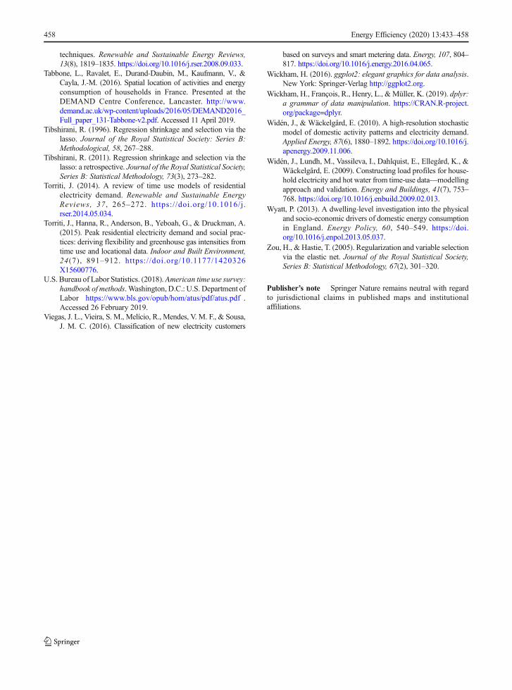
techniques. Renewable and Sustainable Energy Reviews,13(8), 1819–1835. https://doi.org/10.1016/j.rser.2008.09.033.

Tabbone, L., Ravalet, E., Durand-Daubin, M., Kaufmann, V., &Cayla, J.-M. (2016). Spatial location of activities and energyconsumption of households in France. Presented at theDEMAND Centre Conference, Lancaster. http://www.demand.ac.uk/wp-content/uploads/2016/05/DEMAND2016_Full_paper_131-Tabbone-v2.pdf. Accessed 11 April 2019.

Tibshirani, R. (1996). Regression shrinkage and selection via thelasso. Journal of the Royal Statistical Society: Series B:Methodological, 58, 267–288.

Tibshirani, R. (2011). Regression shrinkage and selection via thelasso: a retrospective. Journal of the Royal Statistical Society,Series B: Statistical Methodology, 73(3), 273–282.

Torriti, J. (2014). A review of time use models of residentialelectricity demand. Renewable and Sustainable EnergyReviews, 37 , 265–272. https://doi.org/10.1016/j.rser.2014.05.034.

Torriti, J., Hanna, R., Anderson, B., Yeboah, G., & Druckman, A.(2015). Peak residential electricity demand and social prac-tices: deriving flexibility and greenhouse gas intensities fromtime use and locational data. Indoor and Built Environment,24(7), 891–912. https://doi.org/10.1177/1420326X15600776.

U.S. Bureau of Labor Statistics. (2018). American time use survey:handbook of methods.Washington, D.C.: U.S. Department ofLabor https://www.bls.gov/opub/hom/atus/pdf/atus.pdf .Accessed 26 February 2019.

Viegas, J. L., Vieira, S. M., Melício, R., Mendes, V. M. F., & Sousa,J. M. C. (2016). Classification of new electricity customers

based on surveys and smart metering data. Energy, 107, 804–817. https://doi.org/10.1016/j.energy.2016.04.065.

Wickham, H. (2016). ggplot2: elegant graphics for data analysis.New York: Springer-Verlag http://ggplot2.org.

Wickham, H., François, R., Henry, L., & Müller, K. (2019). dplyr:a grammar of data manipulation. https://CRAN.R-project.org/package=dplyr.

Widén, J., & Wäckelgård, E. (2010). A high-resolution stochasticmodel of domestic activity patterns and electricity demand.Applied Energy, 87(6), 1880–1892. https://doi.org/10.1016/j.apenergy.2009.11.006.

Widén, J., Lundh, M., Vassileva, I., Dahlquist, E., Ellegård, K., &Wäckelgård, E. (2009). Constructing load profiles for house-hold electricity and hot water from time-use data—modellingapproach and validation. Energy and Buildings, 41(7), 753–768. https://doi.org/10.1016/j.enbuild.2009.02.013.

Wyatt, P. (2013). A dwelling-level investigation into the physicaland socio-economic drivers of domestic energy consumptionin England. Energy Policy, 60, 540–549. https://doi.org/10.1016/j.enpol.2013.05.037.

Zou, H., & Hastie, T. (2005). Regularization and variable selectionvia the elastic net. Journal of the Royal Statistical Society,Series B: Statistical Methodology, 67(2), 301–320.

Publisher’s note Springer Nature remains neutral with regardto jurisdictional claims in published maps and institutionalaffiliations.



http://www.demand.ac.uk/wp-content/uploads/2016/05/DEMAND2016_Full_paper_131-Tabbone-v2.pdf





https://doi.org/10.1177/1420326X15600776

https://doi.org/10.1177/1420326X15600776

https://www.bls.gov/opub/hom/atus/pdf/atus.pdf


http://ggplot2.org

https://cran.r-project.org/package=dplyr

https://cran.r-project.org/package=dplyr






daily life and demand: an analysis of intra-day variations

Documents