datamocca - technion

DataMOCCA DATA MOdels for Call Center Analysis

Volume 6.1

Empirical Analysis of Little's law

using Data from the Call Center of USBank

Abir Koren

Professor Avishai Mandelbaum SEElab team:

Dr. Valery Trofimov B.A. Ella Nadjharov M. A. Igor Gavako M.Sc. Katya Kutsi

Created: May 3, 2010

1

DataMOCCA DATA MOdel for Call Center Analysis

The DataMOCCA Project is an initiative of researchers from the Technion—Israel Institute of Technology and The Wharton School—University of Pennsylvania. The mission of the project is to collect, pre-process, organize and analyze data from Telephone Call/Contact Centers. The raw data obtained are call-by-call records of at least one year’s duration from active Call Centers. Among the goals of the project are the development and distribution of Call Center databases, using a uniform schema. The data repository created, together with software tools, will be accessible through the world-wide-web and provide a resource for researchers and teachers of Service Engineering, Science and Management.

List of Documents

Volume Title Revision Date

1 Model Description and Introduction to User Interface July 29, 2006

2 Summary Tables Variable Definitions August, 2006

3.1 SEEStat Guide I – Beginning User to be completed

3.2 SEEStat Guide II – Advanced User July, 2008

3.3 SEEStat Guide III – Data Extraction Facility to be completed

4.1 The Call Center of a “US Bank" November 2, 2006

4.2 The Call Center of “IL Telecom" November 2, 2006

4.3 Empirical Analysis of a Call Center in an Israeli Commercial Company

July, 2009

4.4 Empirical Analysis of a Call Center August, 2009

5.1 Skills-Based-Routing in a US Bank February, 2008

6.1 Empirical Analysis of Little's law using Data from the Call Center of US Bank May, 2010

6.2 Implementing the Offered-Load in SEEStat May, 2011 For more information concerning access to the database and materials please contact: Professor Avishai Mandelbaum: [email protected]

2

mailto:[email protected]

Table of Contents

1 Introduction ........................................................................................................4

2 Brief revision on Little's theorem........................................................................4

3 Measuring the relevant parameters using SEEstat ............................................4

4 Empirical analysis ..............................................................................................5

5 Fitting a new model..........................................................................................10

5.1 Understanding the reasons for Little's formula's failure .............................10

5.2 Revised formula for Little's law..................................................................15

6 New model's relation to time varying Little's law ..............................................17

7 Appendix 1 – The revised formula for the teaching note..................................18

8 Appendix 2 – Trying to fit a different model......................................................21

3

1 Introduction This document concludes an empirical research studying Little's law. The main concept was to calculate the average number of customers in the system (queue, service or both of them) using Little's law and to compare it to the empirical value measured by SEEStat. The first step was to examine various cases using SEEStat and to find out when and under which conditions Little's law applies empirically. Many cases were analyzed using several different time resolutions, which showed that as the resolution gets rougher (bigger intervals) the matching to the empirical measurements gets finer. Among these cases were some that didn't match the measured values under any (standard) resolution. Naturally the next step was to understand the reasons behind these mismatches. Using SEEStat's raw data, I was able to find the sources of the mismatches and to figure how to eliminate their affects. This knowledge enabled us to revise Little's formula to create a better one appropriate to a broader variety of conditions.

2 Brief Revision of Little's Theorem Little's Law is a conservation law for a black-box model of a service system, relating the following three performance measures:

• λ - throughput rate, which is the rate at which customers (service units) flow through (arrive to, depart from) the system;

• L - customer count, which is the number of customers in the system (Work-In-Process);

• W - sojourn time, which is the time that customers spend within the system. In its most widely used version, Little's Law relates the above measures as being steady-state or long-run averages, postulating that L Wλ= × . The law actually binds together the three main players that constitute a service system: the customer, associated with W, which is a measure for operational service quality; the service-provider, concerned withλ , which reflects the server's service effort; and the manager, controlling L, which is a visible proxy for congestion. (The three players are bound via two degrees of freedom.)

3 Measuring the Relevant Parameters Using SEEStat To perform the discussed analysis it is important to understand SEEStat's methods of measuring arrival rate, average waiting time and average number of customers in the system. Arrival rate- practically SEEStat measures arrivals per interval. Each arrival is counted in only one interval according to the arrival (to the system) time. In order to estimate the arrival rate, each value (sum of arrivals per interval) is divided by the interval's size. The division is performed manually.

4

Average waiting time- each arrival brings waiting time ( )0≥ , the waiting time is added to an interval cumulative waiting time according to the arrival time. For each interval the cumulative waiting time is divided by the interval's arrivals. Average customers in system- Each vector contains 86400 cells (one cell per sec) initialized with zeroes. For every arrival the system adds 1 to the vector's cells that matches all the seconds until departure. Using these vectors SEEStat can yield averages for the number of customers in the system.

4 Empirical Analysis Performing the analysis I've used US bank data examining random dates and services. Most of the relevant issues occurred in many cases; hence the examples brought here are limited but essential. According to theory, Little's law takes place under one of 3 circumstances:

1. The examined interval starts and ends with 0 customers in the system. 2. The examined interval starts and ends with the same number of customers, but not

necessarily the same customers. 3. The examined interval takes place when the system is in steady state.

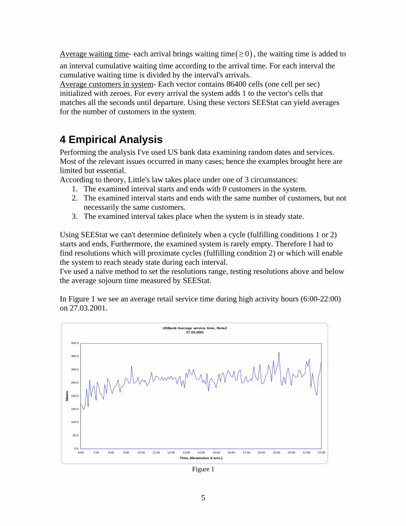
Using SEEStat we can't determine definitely when a cycle (fulfilling conditions 1 or 2) starts and ends, Furthermore, the examined system is rarely empty. Therefore I had to find resolutions which will proximate cycles (fulfilling condition 2) or which will enable the system to reach steady state during each interval. I've used a naïve method to set the resolutions range, testing resolutions above and below the average sojourn time measured by SEEStat. In Figure 1 we see an average retail service time during high activity hours (6:00-22:00) on 27.03.2001.

USBank Average service time, Retail27.03.2001

0.0

50.0

100.0

150.0

200.0

250.0

300.0

350.0

400.0

6:00 7:00 8:00 9:00 10:00 11:00 12:00 13:00 14:00 15:00 16:00 17:00 18:00 19:00 20:00 21:00 22:00

Time (Resolution 6 min.)

Mea

ns

Figure 1

5

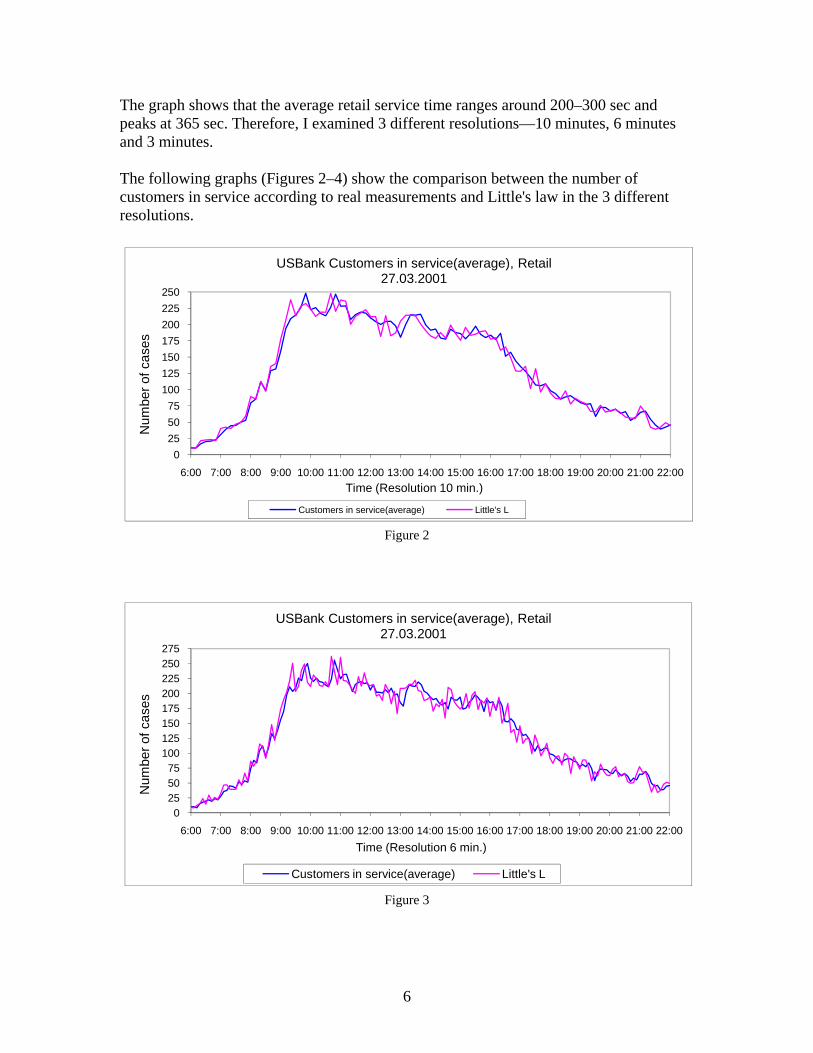
The graph shows that the average retail service time ranges around 200–300 sec and peaks at 365 sec. Therefore, I examined 3 different resolutions—10 minutes, 6 minutes and 3 minutes. The following graphs (Figures 2–4) show the comparison between the number of customers in service according to real measurements and Little's law in the 3 different resolutions.

0255075

100125150175200225250

6:00 7:00 8:00 9:00 10:00 11:00 12:00 13:00 14:00 15:00 16:00 17:00 18:00 19:00 20:00 21:00 22:00

Num

ber o

f cas

es


USBank Customers in service(average), Retail27.03.2001

Customers in service(average) Little's L

Figure 2

0255075

100125150175200225250275

6:00 7:00 8:00 9:00 10:00 11:00 12:00 13:00 14:00 15:00 16:00 17:00 18:00 19:00 20:00 21:00 22:00

Num

ber o

f cas

es




Figure 3

6

0255075

100125150175200225250275

6:00 7:00 8:00 9:00 10:00 11:00 12:00 13:00 14:00 15:00 16:00 17:00 18:00 19:00 20:00 21:00 22:00

Num

ber o

f cas

es




Figure 4 It's easy to see that as the resolution becomes finer, the matching (of the two curves) becomes rougher. Another example of resolution effects is shown by the following graphs (Figures 5–6):

USBank Average wait time(all)02.04.2001

0.0

25.0

50.0

75.0

100.0

125.0

150.0

175.0

200.0

14:00 15:00 16:00 17:00 18:00 19:00 20:00


Mea

ns

Figure 5

We can see there's a peak in the average waiting time between 17:00 to 19:30. The average off-peak waiting time ranges around 10 sec.; during the peak periods, it rises up to 175 sec.

7

USBank Customers in queue(average)02.04.2001

0.0

10.0

20.0

30.0

40.0

50.0

60.0

70.0

80.0

90.0

100.0

110.0

14:00 15:00 16:00 17:00 18:00 19:00 20:00


Num

ber o

f cas

es

Customers in queue(average) Little's L Figure 6

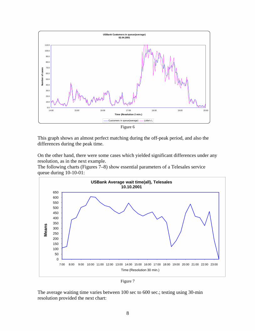
This graph shows an almost perfect matching during the off-peak period, and also the differences during the peak time. On the other hand, there were some cases which yielded significant differences under any resolution, as in the next example. The following charts (Figures 7–8) show essential parameters of a Telesales service queue during 10-10-01:

050

100150200250300350400450500550600650

7:00 8:00 9:00 10:00 11:00 12:00 13:00 14:00 15:00 16:00 17:00 18:00 19:00 20:00 21:00 22:00 23:00

Mea

ns


USBank Average wait time(all), Telesales10.10.2001

Figure 7

The average waiting time varies between 100 sec to 600 sec.; testing using 30-min resolution provided the next chart:

8

USBank Customers in queue(average), Telesales10.10.2001

0.0

25.0

50.0

75.0

100.0

125.0

150.0

175.0

07:00 08:00 09:00 10:00 11:00 12:00 13:00 14:00 15:00 16:00 17:00 18:00 19:00 20:00 21:00 22:00 23:00


Num

ber o

f cas

es

Customers in queue(average) Little

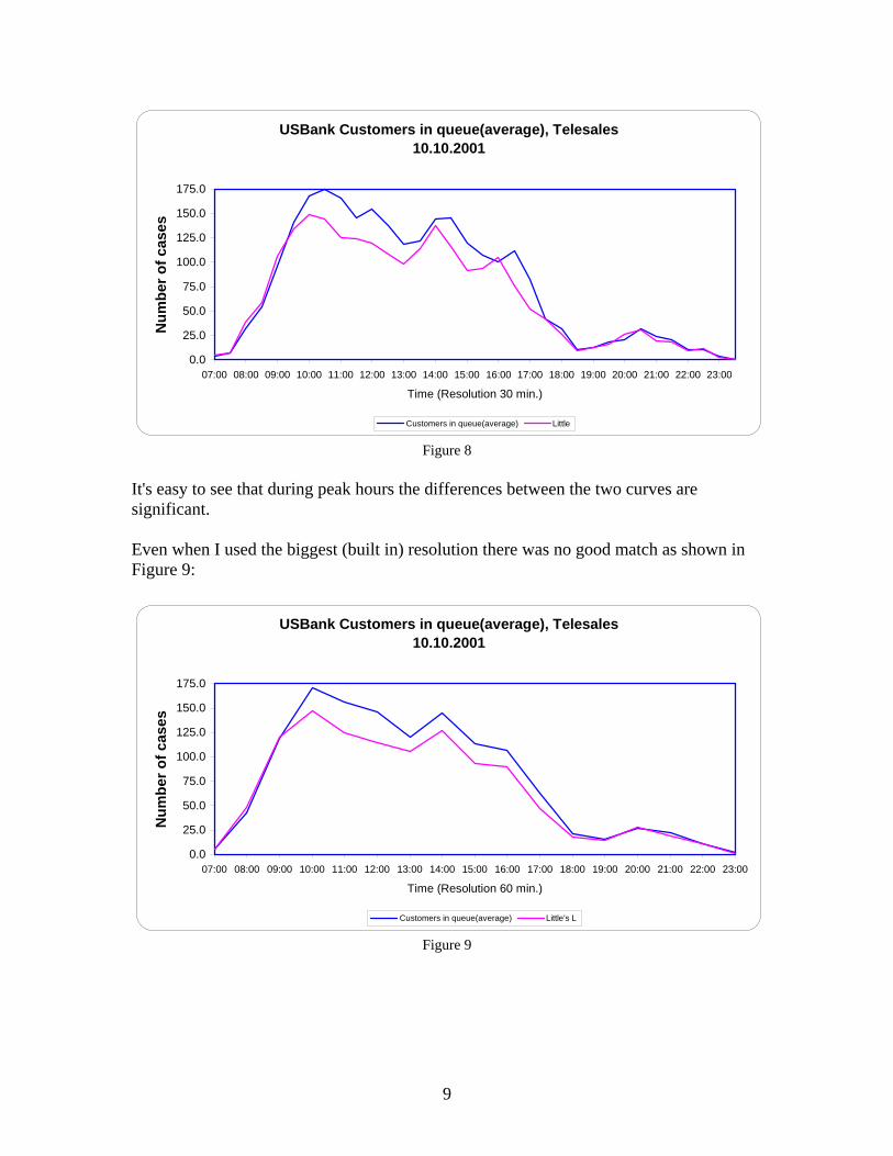
Figure 8 It's easy to see that during peak hours the differences between the two curves are significant. Even when I used the biggest (built in) resolution there was no good match as shown in Figure 9:


0.0

25.0

50.0

75.0

100.0

125.0

150.0

175.0

07:00 08:00 09:00 10:00 11:00 12:00 13:00 14:00 15:00 16:00 17:00 18:00 19:00 20:00 21:00 22:00 23:00


Num

ber o

f cas

es

Customers in queue(average) Little's L

Figure 9

9

5 Fitting a New Model These last findings show that the classic Little's law isn't general enough. Therefore, I wanted to find a model that will describe the relations between the 3 essential parameters in a better way. To find such a model I had to understand when and under what circumstances, Little's formula isn't applicable.

5.1 Understanding the reasons for the failure of Little's formula As shown in the previous section, the calculation to estimate the number of customers in a queue, according to Little's law, on 10-10-01 Telesales service, fails. In this section, I will use this example data.

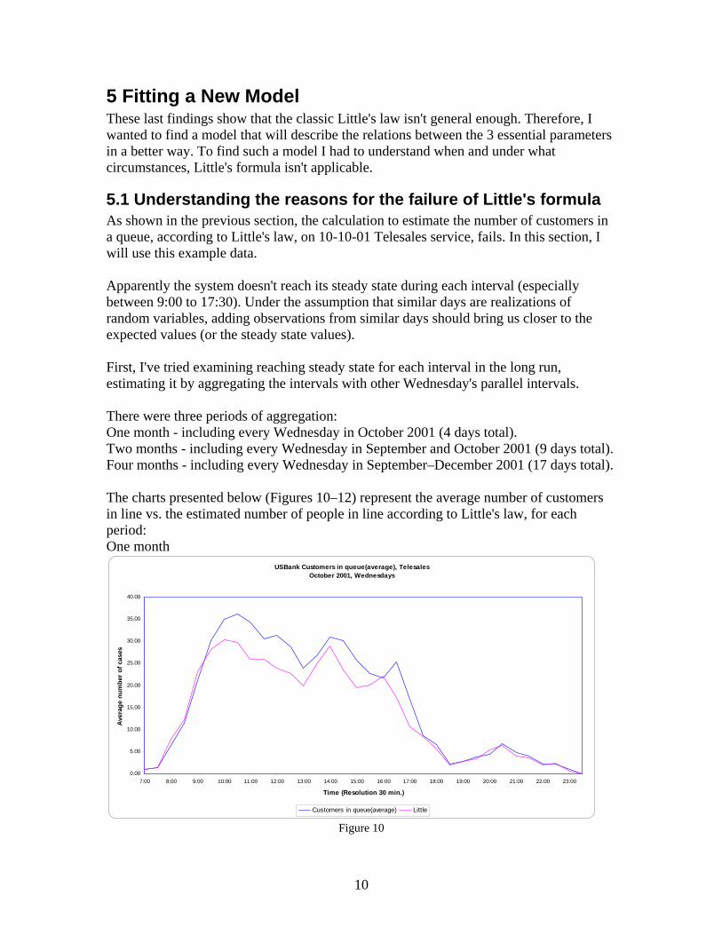
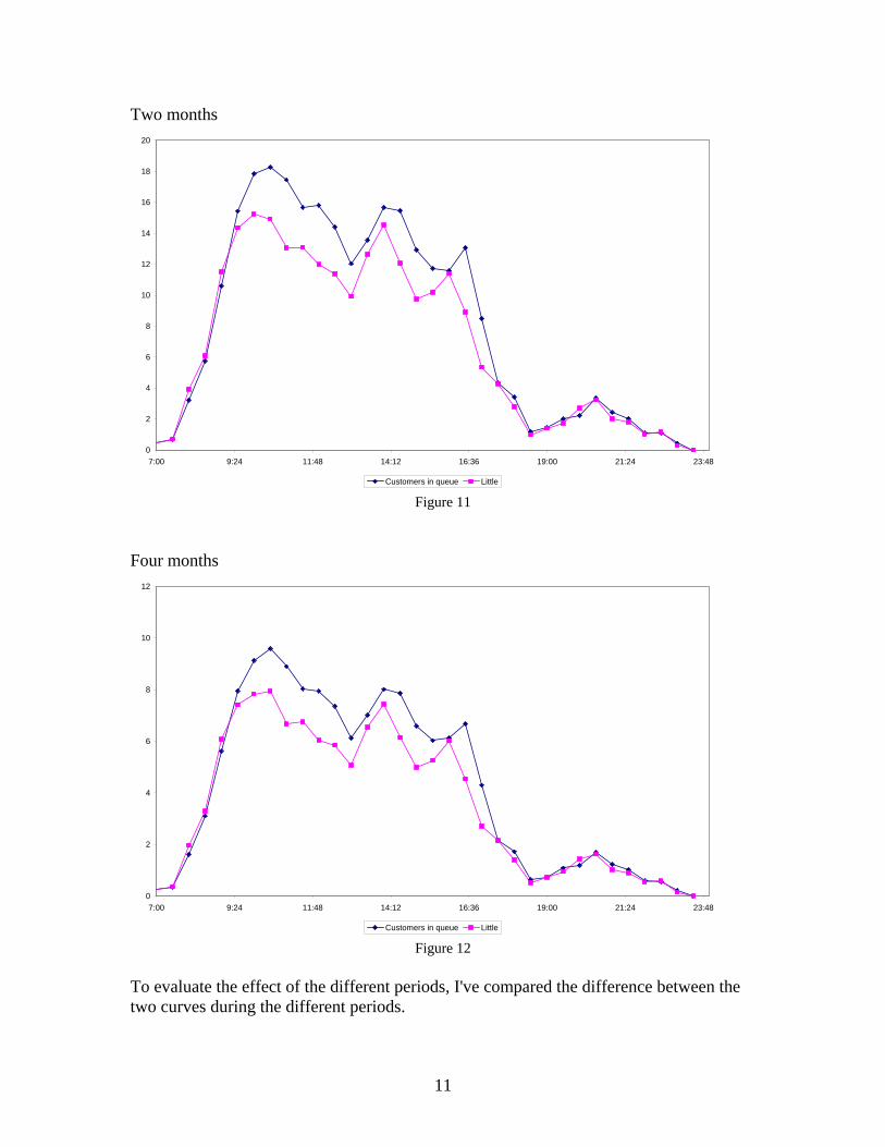
Apparently the system doesn't reach its steady state during each interval (especially between 9:00 to 17:30). Under the assumption that similar days are realizations of random variables, adding observations from similar days should bring us closer to the expected values (or the steady state values). First, I've tried examining reaching steady state for each interval in the long run, estimating it by aggregating the intervals with other Wednesday's parallel intervals. There were three periods of aggregation: One month - including every Wednesday in October 2001 (4 days total). Two months - including every Wednesday in September and October 2001 (9 days total). Four months - including every Wednesday in September–December 2001 (17 days total). The charts presented below (Figures 10–12) represent the average number of customers in line vs. the estimated number of people in line according to Little's law, for each period: One month

USBank Customers in queue(average), TelesalesOctober 2001, Wednesdays

0.00

5.00

10.00

15.00

20.00

25.00

30.00

35.00

40.00

7:00 8:00 9:00 10:00 11:00 12:00 13:00 14:00 15:00 16:00 17:00 18:00 19:00 20:00 21:00 22:00 23:00


Ave

rage

num

ber

of c

ases

Customers in queue(average) Little Figure 10

10

Two months

0

2

4

6

8

10

12

14

16

18

20

7:00 9:24 11:48 14:12 16:36 19:00 21:24 23:48

Customers in queue Little Figure 11

Four months

0

2

4

6

8

10

12

7:00 9:24 11:48 14:12 16:36 19:00 21:24 23:48

Customers in queue Little Figure 12

To evaluate the effect of the different periods, I've compared the difference between the two curves during the different periods.

11

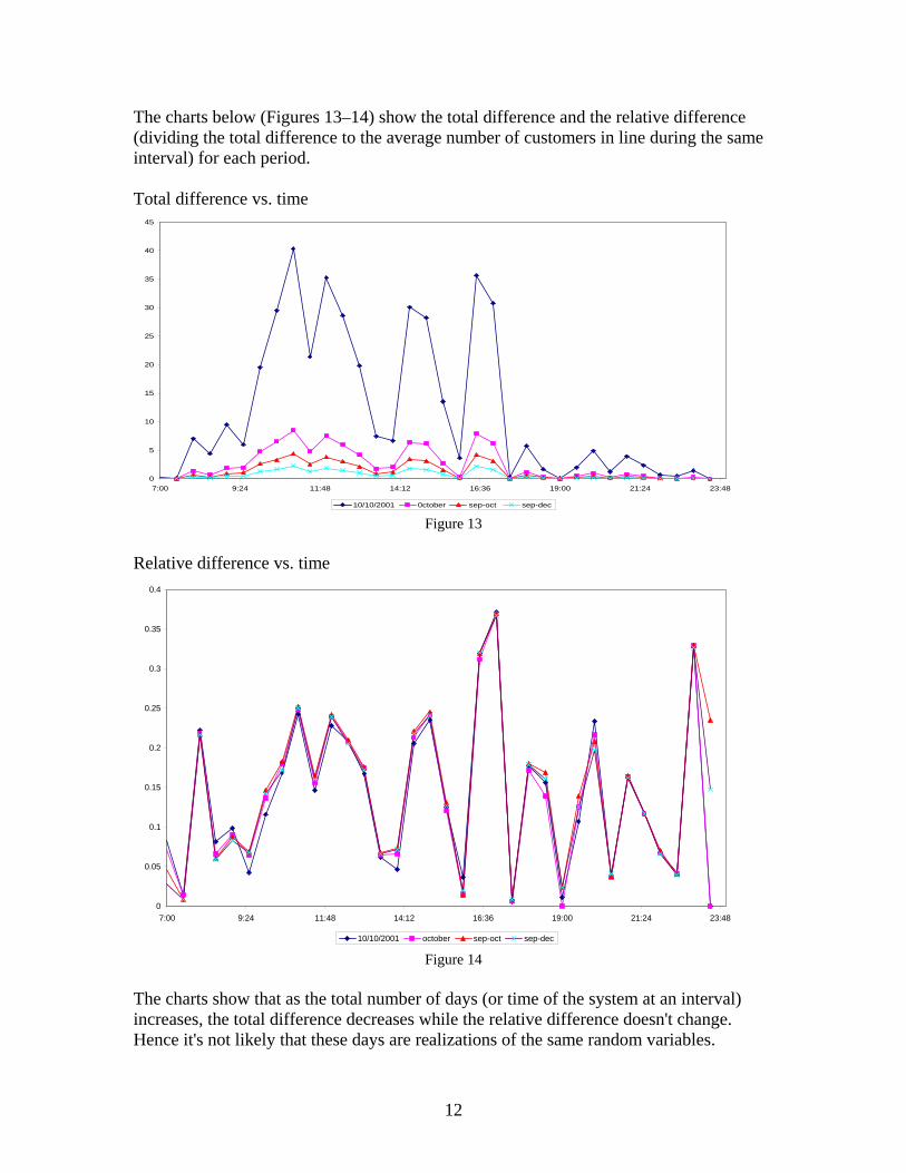
The charts below (Figures 13–14) show the total difference and the relative difference (dividing the total difference to the average number of customers in line during the same interval) for each period. Total difference vs. time

0

5

10

15

20

25

30

35

40

45

7:00 9:24 11:48 14:12 16:36 19:00 21:24 23:48

10/10/2001 0ctober sep-oct sep-dec Figure 13

Relative difference vs. time

0

0.05

0.1

0.15

0.2

0.25

0.3

0.35

0.4

7:00 9:24 11:48 14:12 16:36 19:00 21:24 23:48

10/10/2001 october sep-oct sep-dec Figure 14

The charts show that as the total number of days (or time of the system at an interval) increases, the total difference decreases while the relative difference doesn't change. Hence it's not likely that these days are realizations of the same random variables.

12

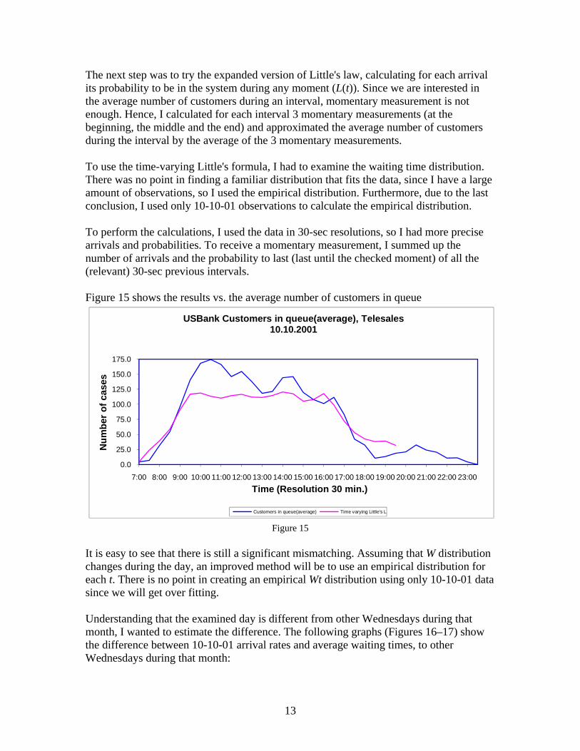
The next step was to try the expanded version of Little's law, calculating for each arrival its probability to be in the system during any moment (L(t)). Since we are interested in the average number of customers during an interval, momentary measurement is not enough. Hence, I calculated for each interval 3 momentary measurements (at the beginning, the middle and the end) and approximated the average number of customers during the interval by the average of the 3 momentary measurements. To use the time-varying Little's formula, I had to examine the waiting time distribution. There was no point in finding a familiar distribution that fits the data, since I have a large amount of observations, so I used the empirical distribution. Furthermore, due to the last conclusion, I used only 10-10-01 observations to calculate the empirical distribution. To perform the calculations, I used the data in 30-sec resolutions, so I had more precise arrivals and probabilities. To receive a momentary measurement, I summed up the number of arrivals and the probability to last (last until the checked moment) of all the (relevant) 30-sec previous intervals. Figure 15 shows the results vs. the average number of customers in queue

0.0

25.0

50.0

75.0

100.0

125.0

150.0

175.0

7:00 8:00 9:00 10:00 11:00 12:00 13:00 14:00 15:00 16:00 17:00 18:00 19:00 20:00 21:00 22:00 23:00

Num

ber o

f cas

es



Customers in queue(average) Time varying Little's L

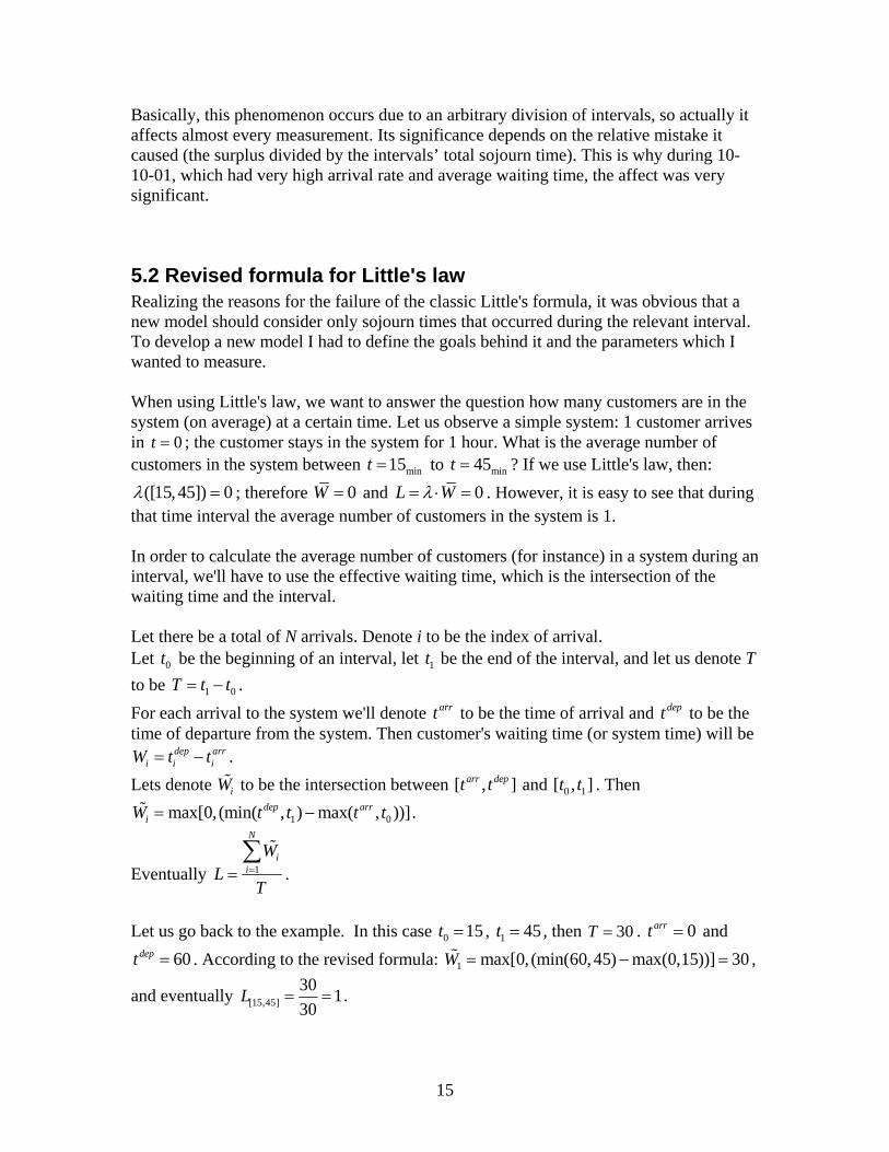
Figure 15 It is easy to see that there is still a significant mismatching. Assuming that W distribution changes during the day, an improved method will be to use an empirical distribution for each t. There is no point in creating an empirical Wt distribution using only 10-10-01 data since we will get over fitting. Understanding that the examined day is different from other Wednesdays during that month, I wanted to estimate the difference. The following graphs (Figures 16–17) show the difference between 10-10-01 arrival rates and average waiting times, to other Wednesdays during that month:

13

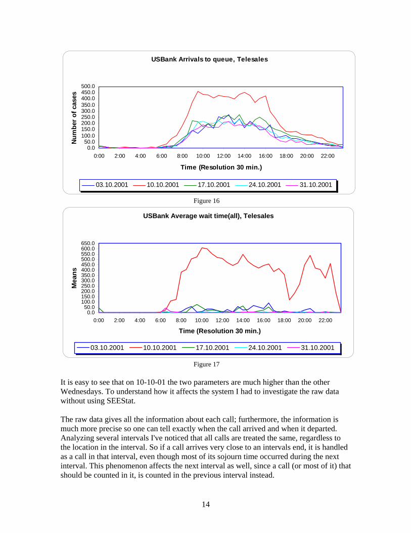
USBank Arrivals to queue, Telesales

0.050.0

100.0150.0200.0250.0300.0350.0400.0450.0500.0

0:00 2:00 4:00 6:00 8:00 10:00 12:00 14:00 16:00 18:00 20:00 22:00


Num

ber o

f cas

es

03.10.2001 10.10.2001 17.10.2001 24.10.2001 31.10.2001

Figure 16

USBank Average wait time(all), Telesales

0.050.0

100.0150.0200.0250.0300.0350.0400.0450.0500.0550.0600.0650.0

0:00 2:00 4:00 6:00 8:00 10:00 12:00 14:00 16:00 18:00 20:00 22:00


Mea

ns

03.10.2001 10.10.2001 17.10.2001 24.10.2001 31.10.2001

Figure 17 It is easy to see that on 10-10-01 the two parameters are much higher than the other Wednesdays. To understand how it affects the system I had to investigate the raw data without using SEEStat. The raw data gives all the information about each call; furthermore, the information is much more precise so one can tell exactly when the call arrived and when it departed. Analyzing several intervals I've noticed that all calls are treated the same, regardless to the location in the interval. So if a call arrives very close to an intervals end, it is handled as a call in that interval, even though most of its sojourn time occurred during the next interval. This phenomenon affects the next interval as well, since a call (or most of it) that should be counted in it, is counted in the previous interval instead.

14

Basically, this phenomenon occurs due to an arbitrary division of intervals, so actually it affects almost every measurement. Its significance depends on the relative mistake it caused (the surplus divided by the intervals’ total sojourn time). This is why during 10-10-01, which had very high arrival rate and average waiting time, the affect was very significant.

5.2 Revised formula for Little's law Realizing the reasons for the failure of the classic Little's formula, it was obvious that a new model should consider only sojourn times that occurred during the relevant interval. To develop a new model I had to define the goals behind it and the parameters which I wanted to measure. When using Little's law, we want to answer the question how many customers are in the system (on average) at a certain time. Let us observe a simple system: 1 customer arrives in ; the customer stays in the system for 1 hour. What is the average number of customers in the system between

0t =min15t = to min45t = ? If we use Little's law, then:

([15,45]) 0λ = ; therefore 0W = and 0L Wλ= ⋅ = . However, it is easy to see that during that time interval the average number of customers in the system is 1. In order to calculate the average number of customers (for instance) in a system during an interval, we'll have to use the effective waiting time, which is the intersection of the waiting time and the interval. Let there be a total of N arrivals. Denote i to be the index of arrival. Let be the beginning of an interval, let be the end of the interval, and let us denote T to be .

0t 1t

1 0T t t= −

For each arrival to the system we'll denote to be the time of arrival and to be the time of departure from the system. Then customer's waiting time (or system time) will be

.

arrt dept

dep arri i iW t t= −

Lets denote to be the intersection between [ , and . Then .

iW% ]t

arr dept t 0 1[ , ]t t

1 0max[0, (min( , ) max( , ))]dep arriW t t t= −%

Eventually 1

N

ii

WL

T==∑ %

.

Let us go back to the example. In this case 0 15t = , 1 45t = , then 30T = . and

. According to the revised formula: 0arrt =

60dept = 1 max[0, (min(60,45) max(0,15))] 30W = − =% ,

and eventually [15,45]30 130

L = = .

15

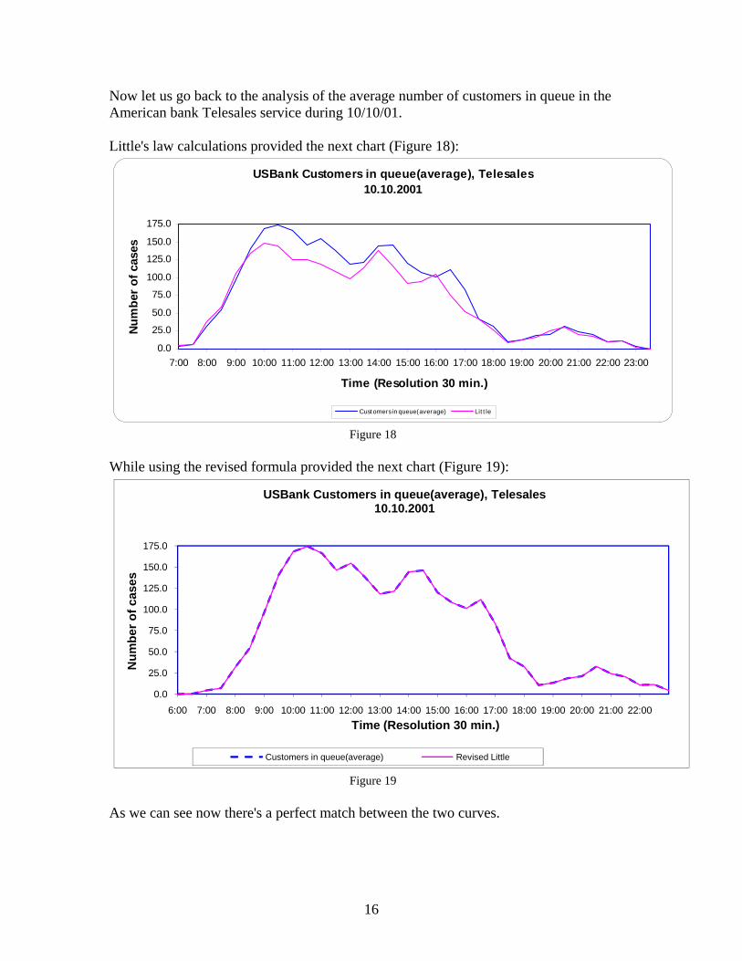
Now let us go back to the analysis of the average number of customers in queue in the American bank Telesales service during 10/10/01. Little's law calculations provided the next chart (Figure 18):


0.0

25.0

50.0

75.0

100.0

125.0

150.0

175.0

7:00 8:00 9:00 10:00 11:00 12:00 13:00 14:00 15:00 16:00 17:00 18:00 19:00 20:00 21:00 22:00 23:00


Num

ber o

f cas

es

Cust omers in queue(average) Lit t le

Figure 18 While using the revised formula provided the next chart (Figure 19):

0.0

25.0

50.0

75.0

100.0

125.0

150.0

175.0

6:00 7:00 8:00 9:00 10:00 11:00 12:00 13:00 14:00 15:00 16:00 17:00 18:00 19:00 20:00 21:00 22:00

Num

ber o

f cas

es



Customers in queue(average) Revised Little

Figure 19 As we can see now there's a perfect match between the two curves.

16

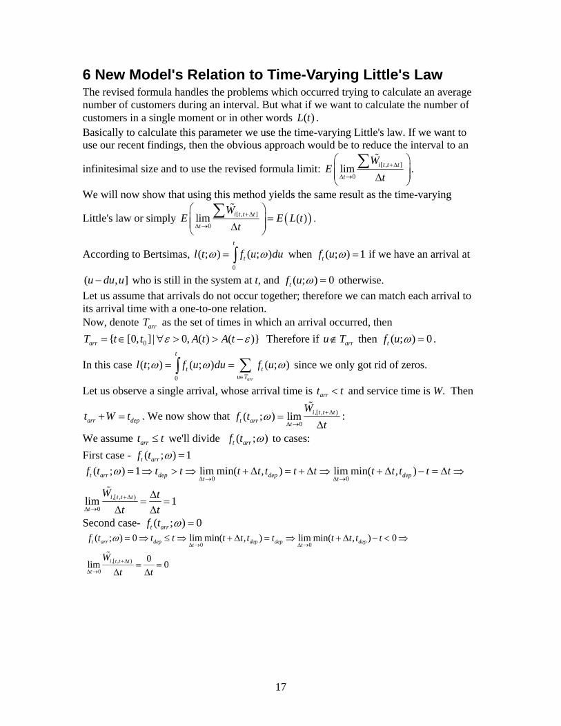
6 New Model's Relation to Time-Varying Little's Law The revised formula handles the problems which occurred trying to calculate an average number of customers during an interval. But what if we want to calculate the number of customers in a single moment or in other words . ( )L tBasically to calculate this parameter we use the time-varying Little's law. If we want to use our recent findings, then the obvious approach would be to reduce the interval to an

infinitesimal size and to use the revised formula limit: [ , ]

0lim i t t t

t

WE

t+Δ

Δ →

⎛ ⎞⎜ ⎟⎜ ⎟Δ⎝ ⎠

∑ %.

We will now show that using this method yields the same result as the time-varying

Little's law or simply ( )[ , ]

0lim ( )i t t t

t

WE E

t+Δ

Δ →

⎛ ⎞=⎜ ⎟⎜ ⎟Δ⎝ ⎠

∑ %L t .

According to Bertsimas, when 0

( ; ) ( ; )t

tl t f u duω ω= ∫ ( ; ) 1tf u ω = if we have an arrival at

who is still in the system at t, and ( ,u du u− ] ( ; ) 0tf u ω = otherwise. Let us assume that arrivals do not occur together; therefore we can match each arrival to its arrival time with a one-to-one relation. Now, denote as the set of times in which an arrival occurred, then arrT

0{ [0, ] | 0, ( ) ( )}arrT t t A t A tε ε= ∈ ∀ > > − Therefore if arru T∉ then ( ; ) 0tf u ω = .

In this case 0

( ; ) ( ; ) ( ; )arr

t

tu T

l t f u du f utω ω∈

= = ∑∫ ω

t

since we only got rid of zeros.

Let us observe a single arrival, whose arrival time is arrt < and service time is W. Then

. We now show that arr dept W t+ = ,[ , )

0( ; ) lim i t t t

t arr t

Wf t

tω +Δ

Δ →=

Δ

%:

We assume we'll divide arrt ≤ t ( ; )t arrf t ω to cases: First case - ( ; ) 1t arrf t ω =

0 0

,[ , )

0

( ; ) 1 lim min( , ) lim min( , )

lim 1

t arr dep dep dept t

i t t t

t

f t t t t t t t t t t t t t

W tt t

ωΔ → Δ →

+Δ

Δ →

= ⇒ > ⇒ +Δ = + Δ ⇒ +Δ − = Δ ⇒

Δ= =

Δ Δ

%

Second case- ( ; ) 0t arrf t ω =

0 0

,[ , )

0

( ; ) 0 lim min( , ) lim min( , ) 0

0lim 0

t arr dep dep dep dept t

i t t t

t

f t t t t t t t t t t t

Wt t

ωΔ → Δ →

+Δ

Δ →

= ⇒ ≤ ⇒ +Δ = ⇒ +Δ − < ⇒

= =Δ Δ

%

17

Then ,[ , )

00

( ; ) ( ; ) ( ; ) limarr

ti t t t

t t tu T i I

Wl t f u du f u

tω ω ω +Δ

Δ →∈ ∈

= = =Δ∑ ∑∫

% for every realization, hence

( )[ , ]

0lim ( )i t t t

t

WE E

t+Δ

Δ →

⎛ ⎞=⎜ ⎟⎜ ⎟Δ⎝ ⎠

∑ %L t .

A practical way to calculate it would be to choose tΔ to be smaller than the smallest unit of measurement, and not use the limit. For instance, if the system's smallest resolution is

1 sec, and 0.5 sec is small enough to be used as tΔ , then we get ( )[ , 0.5]

0.5i t tW

L t+ =∑ % for

each realization.

7 Appendix 1 – The Revised Formula for the Teaching Note What happens if the system doesn't satisfy the mentioned conditions for Little's formula? Consider a system with one permanent customer (i.e. arrival time < 0W ). = ∞Then for every 0T ≥ 0λ = , W=0. Using Little's formula we get:

0 0 0L Wλ= ⋅ = ⋅ = for every . 0T ≥ Recall that L was defined as a number in the system, so Little's formula suggests that there are 0 customers in the system. But we defined the system to have one permanent customer so obviously . 1 0L = ≠The reason for the difference is that the system doesn't satisfy Little's formula's pre-conditions. Practically there are three common cases:

1) Arriving before the beginning of the examined interval, and staying in the system during the examined interval.

2) Arriving during the examined interval, and staying in the system after the end of the examined interval.

3) Arriving before the beginning of the examined interval, and staying in the system after the end of the examined interval.

Let's observe a simple example to describe it: Consider a "black box" system, which starts at 0t = . We will examine the system between to . For simplicity we consider only one arrival with

. We'll handle three arrival times 3hourst = 4hourst =

2hoursW = 2arr hourst = , 3.5arr hourst = and according to cases 1, 2 and 3, respectively.

2.5arr hourst =

The first case:

18

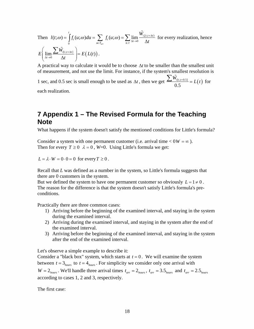
0λ = since there were no arrivals during the interval, hence 0hoursW = and therefore L=0. But if we represent it graphically:

It's easy to see that (where S is the shaded area in the interval) and therefore 1 0S = ≠

1 1 01

SLT

= = = ≠ .

A(t)

Time t=3 t=4t=2

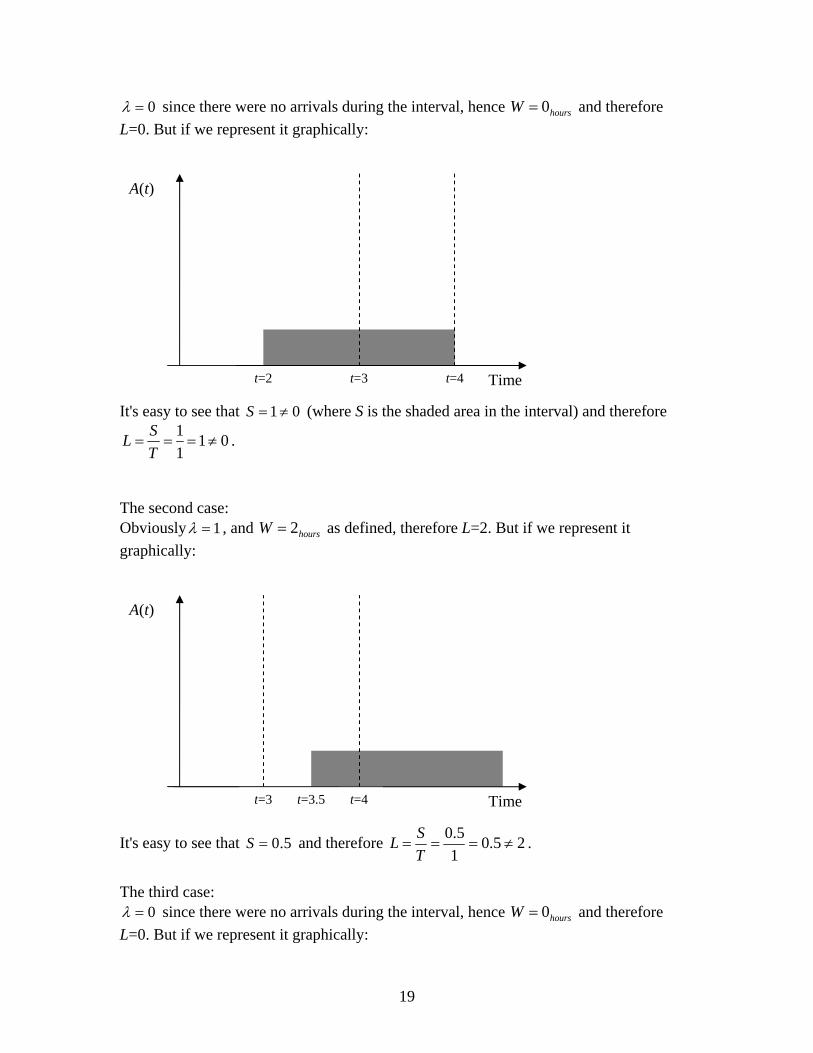
The second case: Obviously 1λ = , and as defined, therefore L=2. But if we represent it graphically:

It's easy to see that and therefore

2hoursW =

0.5S =0.5 0.5 21

SLT

= = = ≠ .

A(t)

Time t=3.5 t=4t=3

The third case:

0λ = since there were no arrivals during the interval, hence 0hoursW = and therefore L=0. But if we represent it graphically:

19

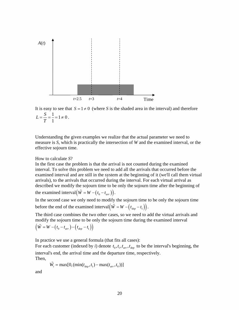
It is easy to see that (where S is the shaded area in the interval) and therefore 1 0S = ≠

1 1 01

SLT

= = = ≠ .

A(t)

Time t=3 t=4t=2.5

Understanding the given examples we realize that the actual parameter we need to measure is S, which is practically the intersection of W and the examined interval, or the effective sojourn time. How to calculate S? In the first case the problem is that the arrival is not counted during the examined interval. To solve this problem we need to add all the arrivals that occurred before the examined interval and are still in the system at the beginning of it (we'll call them virtual arrivals), to the arrivals that occurred during the interval. For each virtual arrival as described we modify the sojourn time to be only the sojourn time after the beginning of the examined interval . ( )( )0 arrW W t t= − −%

In the second case we only need to modify the sojourn time to be only the sojourn time before the end of the examined interval ( )( )1depW W t t= − −% .

The third case combines the two other cases, so we need to add the virtual arrivals and modify the sojourn time to be only the sojourn time during the examined interval

( ) ( )( )0 1arr depW W t t t t= − − − −%

In practice we use a general formula (that fits all cases): For each customer (indexed by i) denote to be the interval's beginning, the interval's end, the arrival time and the departure time, respectively.

0 1, , ,arr dept t t t

Then, 1 0max[0, (min( , ) max( , ))]i dep arrW t t t= −% tand

20

0 , 0 ,( ) ( )arr i dep ii I

0A t I t t t∈

= < ∧∑% t> ;

eventually

( )1 0

1 0

( ) ( ) ( )0A t A t A tt t

λ− +

=−

%% ,

( 0

ii I

ii I

WW

I W∈

∈

=>

∑∑

%

%% )

and now L Wλ= ⋅% % . Let's go back to the examples: In the first case. 0 13, 4, 2, 4arr dept t t t= = = =Then

( ) ( )( ) ( )max 0, min 4, 4 max 2,3 max 0,1 1W ⎡ ⎤= − =⎣ ⎦% = ,

( )0

1 1 1( ) 1 1

1A t λ

− += → = =% % , and hence

1 1 1L = ⋅ = , as we figured from the graph.

In the second case . 0 13, 4, 3.5, 5.5arr dept t t t= = = =Then

( ) ( )( ) ( )max 0, min 4,5.5 max 3.5,3 max 0,0.5 0.5W ⎡ ⎤= − =⎣ ⎦% = ,

( )0

1 0 0( ) 0 1

1A t λ

− += → = =% % , and hence

1 0.5 0.5L = ⋅ = , as we figured from the graph. In conclusion, we modified the arrivals to satisfy Little's formula conditions for any interval. This modification practically simulated systems starting empty and ending empty, and thus expanded Little's formula to a more general form.

8 Appendix 2 – Trying to Fit a Different Model To be more accurate I tried to measure the offered load per interval vs. the system's dynamic capacity for the same interval. I've created two variables in SEEStat—the first one holds the total amount of "service time" entered into the system for each interval (the service doesn't have to take place at that interval), and the second variable holds the total amount of "service time" that took place at the interval. For each interval I've calculated the difference between the two variables and then summed it up for each interval (eventually it shows the total "service time surplus" for each interval).

21

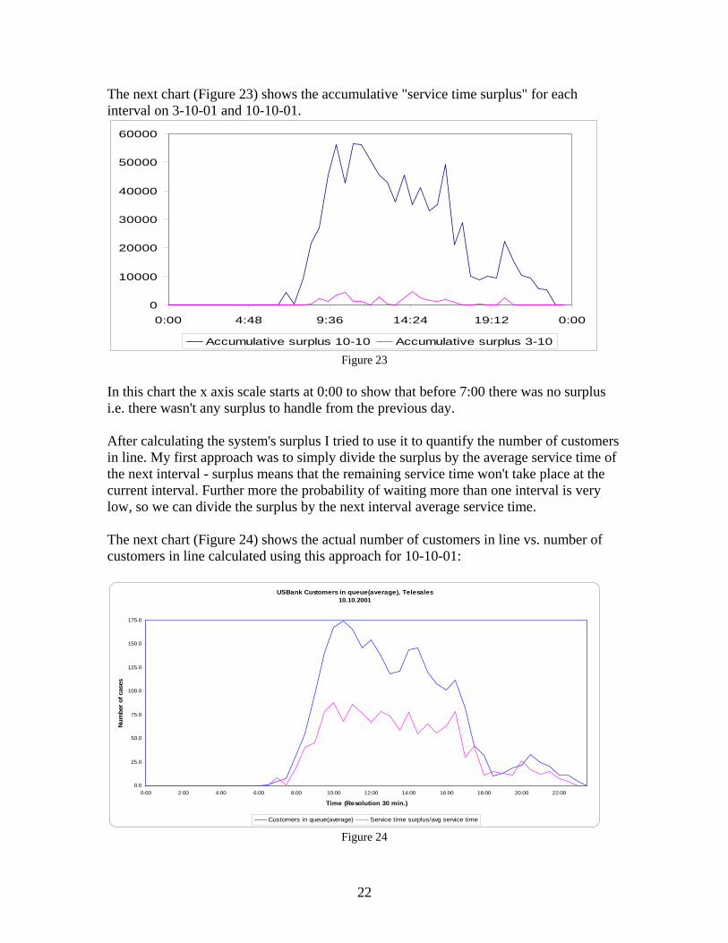
The next chart (Figure 23) shows the accumulative "service time surplus" for each interval on 3-10-01 and 10-10-01.

0

10000

20000

30000

40000

50000

60000

0:00 4:48 9:36 14:24 19:12 0:00

Accumulative surplus 10-10 Accumulative surplus 3-10 Figure 23

In this chart the x axis scale starts at 0:00 to show that before 7:00 there was no surplus i.e. there wasn't any surplus to handle from the previous day. After calculating the system's surplus I tried to use it to quantify the number of customers in line. My first approach was to simply divide the surplus by the average service time of the next interval - surplus means that the remaining service time won't take place at the current interval. Further more the probability of waiting more than one interval is very low, so we can divide the surplus by the next interval average service time. The next chart (Figure 24) shows the actual number of customers in line vs. number of customers in line calculated using this approach for 10-10-01:


0.0

25.0

50.0

75.0

100.0

125.0

150.0

175.0

0:00 2:00 4:00 6:00 8:00 10:00 12:00 14:00 16:00 18:00 20:00 22:00


Num

ber

of c

ases

Customers in queue(average) Service time surplus/avg service time Figure 24

22

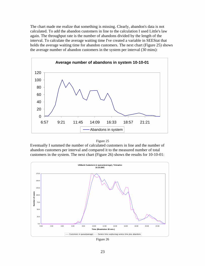
The chart made me realize that something is missing. Clearly, abandon's data is not calculated. To add the abandon customers in line to the calculation I used Little's law again. The throughput rate is the number of abandons divided by the length of the interval. To calculate the average waiting time I've created a variable in SEEStat that holds the average waiting time for abandon customers. The next chart (Figure 25) shows the average number of abandon customers in the system per interval (30 mins):

0

20

40

60

80

100

120

6:57 9:21 11:45 14:09 16:33 18:57 21:21

Average number of abandons in system 10-10-01

Abandons in system

Figure 25

Eventually I summed the number of calculated customers in line and the number of abandon customers per interval and compared it to the measured number of total customers in the system. The next chart (Figure 26) shows the results for 10-10-01:


0.0

25.0

50.0

75.0

100.0

125.0

150.0

175.0

0:00 2:00 4:00 6:00 8:00 10:00 12:00 14:00 16:00 18:00 20:00 22:00


Num

ber o

f cas

es

Customers in queue(average) Service time surplus/avg service time plus abandons Figure 26

23

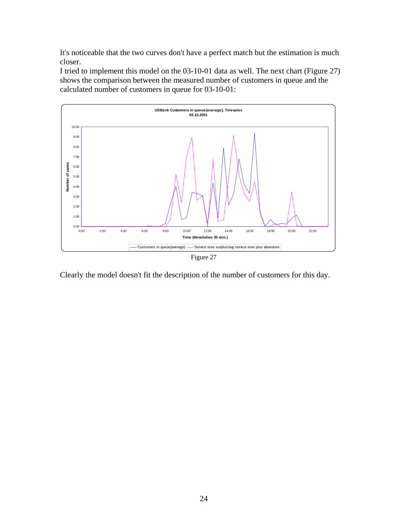
It's noticeable that the two curves don't have a perfect match but the estimation is much closer. I tried to implement this model on the 03-10-01 data as well. The next chart (Figure 27) shows the comparison between the measured number of customers in queue and the calculated number of customers in queue for 03-10-01:


0.00

1.00

2.00

3.00

4.00

5.00

6.00

7.00

8.00

9.00

10.00

0:00 2:00 4:00 6:00 8:00 10:00 12:00 14:00 16:00 18:00 20:00 22:00


Num

ber o

f cas

es

Customers in queue(average) Service time surplus/avg service time plus abandons Figure 27

Clearly the model doesn't fit the description of the number of customers for this day.

24