workload flurries - technion
TRANSCRIPT
Workload Flurries
Dan Tsafrir Dror G. FeitelsonSchool of Computer Science and Engineering
The Hebrew University of Jerusalem91904 Jerusalem, Israel
Abstract
The performance of computer systems depends, among other things, on the workload. Performanceevaluations are therefore often done using logs of workloads on current productions systems, under theassumption that such real workloads are representative and reliable; likewise, workload modeling is typ-ically based on real workloads. However, real workloads may also contain anomalies that make themnon-representative and unreliable. A previously unrecognized type of anomaly is workload flurries:surges of activity with a repetitive nature, caused by a single user, that dominate the workload for a rel-atively short period. Under suitable conditions, such flurries can have a decisive effect on performanceevaluation results. The problem is that workloads containing such a flurry are not representative of nor-mal usage. Moreover, creating a statistical model based on such a workload or using it directly is also notrepresentative of flurries in general. This motivates the approach of identifying and removing the flurries,so as to allow for an evaluation under normal conditions. We demonstrate this for several evaluationsof parallel systems, showing that the anomalies in the workload as embodied by flurries carry over toanomalies in the evaluation results, which disappear when the flurries are removed. Such an evaluationcan then be augmented by a separate evaluation of the deviation caused by the flurry.
Categories and subject descriptors: C.4 [Performance of Systems], K.6.2 [Installation Management]:Performance and usage measurement.
General terms: Experimentation, Measurement, Performance.
Additional Key Words and Phrases: Computer workload, User behavior, Abnormal workload, Represen-tative workload, Data sanitation.
1 Introduction
The performance of a computer system depends not only on its design and implementation, but also on theworkload to which it is subjected [11]. Different workloads may lead to different absolute performance num-bers, and in some cases to different relative ranking of systems or designs. Using representative workloadsis therefore crucial in order to obtain reliable performance evaluation results.
One way to obtain representative workloads is to use real workloads from productions systems. If acurrent system is available that has a similar functionality to the system being evaluated, one can assumethat the same workload may apply. One can then record the workload on the current system, and play backthe recording to drive a simulation of the new system. Alternatively, the recorded workload can be usedas the basis for constructing a workload model (e.g. [17, 9, 22]). This has the benefit of allowing for moreflexible usage, e.g. by modifying model parameters so as to adapt it to different system configurations.
However, using recorded workloads also has its problems. It is well known that workloads at differentinstallations differ, and that workloads evolve with time as users learn to better use the system [16]. Thispaper deals with a different type of drawback: real workloads may contain abnormal behaviors that, though
1
they do in fact occur on rare occasions, are not representative in general. Workload flurries are such events.They consist of huge surges of activity by single users that dominate the workload for a limited time.
Workload flurries have two types of effects on performance evaluation. One is in the context of workloadmodeling, and specifically the fitting of statistical distributions to workload data. The existence of a flurrymay alter workload statistics, leading to the use of un-representative values by an unwary analyst. The otheris an effect on performance evaluation results when using a workload trace to drive a simulation. Flurriesmay be very sensitive to the details of the system’s behavior, so extremely small modifications may lead tolarge effects that are not reliable predictors of real performance. We demonstrate both effects in the contextof workloads on parallel supercomputers.
The contributions of this paper are the following:
• The identification of workload flurries as an important phenomenon, independent of other workloadfeatures that have been recognized in the past (Sections 3 and 4).
• Showing that the existence of workload flurries can taint workload modeling, leading to models thatare actually non-representative and overly complex. For example, distributions of workload param-eters that seem different in successive years actually only differ due to the flurries that are included(Section 5).
• Showing that workload flurries may cause system evaluations to be extremely sensitive to minor de-tails, because the whole flurry reacts to a change en masse and thereby amplifies its effect. Section 6relates an example where changing the runtime of one job in 67,667 by 30 seconds (relative to a totalruntime of 18 hours) caused the average bounded slowdown of all the jobs to change by about 8%,because of its effect on a subsequent 375-job flurry.
• Showing that noisy or inconsistent evaluation results can be traced to the effect of flurries (severalexamples are given in Section 7).
• Suggesting that the best way to deal with flurries is to carefully identify and remove them (Section 8).This allows for a more reliable evaluation of normal, non-flurry conditions; a separate evaluation canthen be performed to assess the potential impact of flurries. While such data sanitation has been donein the past (e.g. [9]), understanding the characteristics and behavior of flurries will make it easier toapply.
2 Data Sanitation
The need to use representative workloads for system evaluations has long been recognized, and has led tothe practice of monitoring existing systems and characterizing their workloads for this purpose [15, 1]. Butusing workload traces “as is” is a risky business, as they may include various sorts of anomalous behavior.Previous work has focused on analyzing the workload as a whole, and trying to determine whether it isstationary and representative. We suggest a complementary approach in which the data is “cleaned up” byremoving the non-representative parts, and only the remaining data is used in the evaluation.
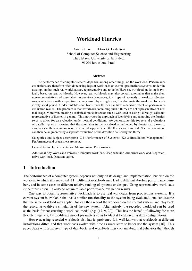
One striking example was reported in the analysis of the workload on the NASA Ames iPSC/860 hy-percube [12]. The histogram of job sizes on that 128-node machine indicated that more than half of the jobswere serial; moreover, most of the serial jobs were flagged as being run by the system support staff (Fig.1). This was a result of an ad-hoc method used to verify that the system was operational and responsiveby running the Unix pwd command on a single node. Overall, a full 56.8% of the trace (24025 jobs) weresuch check-runs. It is quite obvious that these jobs should be removed if the trace is used to analyze parallelworkloads or to evaluate parallel job schedulers.
2
28000
29000
job size1 2 4 8 16 32 64 128
num
ber o
f job
s
0
1000
2000
3000
4000
systemweekendnightday
Figure 1: Histogram of job sizes from the NASA Ames iPSC/860, showing abnormally many single-node systemjobs.
LANL CM−5
time of day0 4 8 12 16 20 24
jobs
per
30
min
0
1000
2000
3000
4000
5000
6000
7000
CTC SP2
time of day0 4 8 12 16 20 24
jobs
per
30
min
0
500
1000
1500
2000
2500
3000
3500
SDSC Blue Horizon
time of day0 4 8 12 16 20 24
jobs
per
30
min
0
1500
3000
4500
6000
7500
9000
SDSC Paragon
time of day0 4 8 12 16 20 24
jobs
per
30
min
0
1000
2000
3000
4000
5000
6000
7000
8000
9000
10000
SDSC SP2
time of day0 4 8 12 16 20 24
jobs
per
30
min
0
400
800
1200
1600
2000
2400
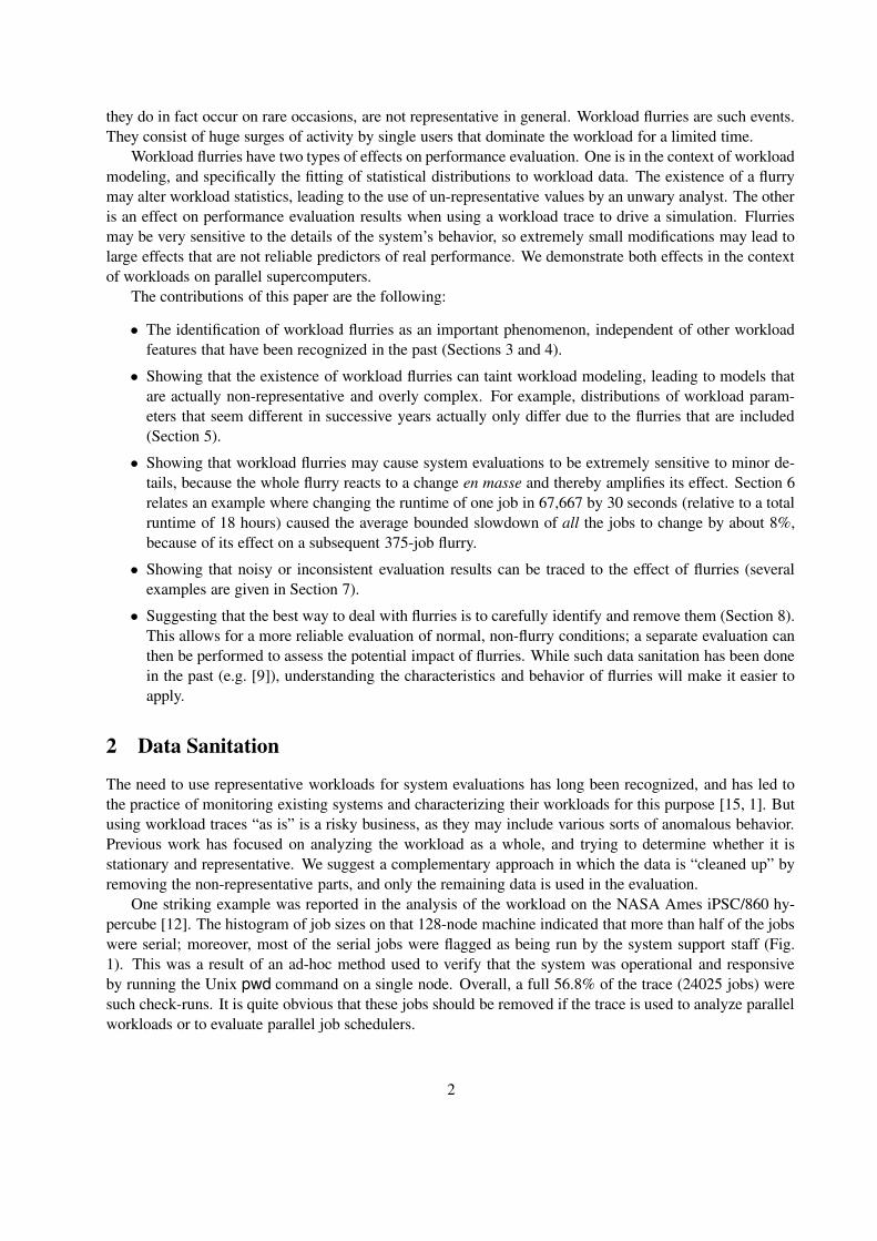
Figure 2: Daily arrival pattern on 5 parallel supercomputers, showing abnormal spike at 3:30 AM on the SDSCParagon.
3
Another example is shown in Fig. 2. This compares the daily arrival cycle on 5 different parallel su-percomputers. All display the expected periodic behavior, with load peaking during work hours and lowerloads at night. But the SDSC Paragon machine has an additional and much higher peak between 3:30 and4:00 AM. Upon investigation, it turned out that a set of 16 jobs with an distinct profile was executed duringthis time slice every day. While specific information is not available, it is reasonable to assume that thesejobs served some system administration function and were executed automatically. It is again obvious thatthey should be removed when using the log for evaluations, so as to reduce the danger of optimizing for thisabnormal behavior.
The above two examples were identified by manual inspection of the workload traces. Obviously, it isdesirable to be able to perform data sanitation automatically. There seems to have been very little work onthis in the past. One example is the proposal by Cirne and Berman [9]. They noticed that workload logssometimes contain periods that are highly abnormal, and suggested that such periods should be deleted.Their methodology was to partition the log into days, and characterize each day’s workload by a vector oflength n (specifically, this was applied to the modeling of the daily arrival cycle, and the vector containedthe coefficients of a polynomial describing it). The days are then clustered into two clusters in Rn. If one ofthe clusters turned out to contain a single day, that day was deleted, and the process was repeated. However,this approach would not catch the two examples cited above, which occur across the whole log.
Workload flurries, to be defined and exemplified in the next section, are also candidates for data sanita-tion. However, this is much less obvious than for the examples cited above.
3 The Phenomenon of Workload Flurries
We define a workload flurry to be a pattern of activity with the following characteristics:
1. It causes a level of activity that is significantly higher than usual, thus dominating the workload
2. It exists for a limited period of time
3. It significantly changes the distributions of workload attributes
4. It is caused by a single user.
The name “workload flurry” derives from the first and second attributes, and from the fact that the itemsconstituting the flurry are typically lightweight, because otherwise the system would be overwhelmed bytheir numbers.
3.1 Observation of Flurries on Parallel Supercomputers
The above definition is derived from observations of such phenomena in the long-term workloads experi-enced by large-scale production parallel supercomputers. While most of the following demonstrations anddiscussion are in the context of parallel systems, we believe that the phenomenon of workload flurries ismuch more wide spread, and provide some additional examples and generalizations in Section 8.1.
Workload data from several large-scale parallel supercomputers is available in the Parallel WorkloadsArchive [25]. We use data (including job arrivals, runtimes, sizes, etc.) from five different installations, andfrom different times, as summarized in Table 1. Dozens of research papers have used these and a few otherlogs as the basis of their evaluations of scheduling mechanisms, oblivious to the fact they contain flurriesthat might significantly distort the results.
Fig. 3 shows the job load (the number of jobs submitted) as a function of time, at the granularity ofweeks. In all five logs, large flurries are observed. They range in size from double the average activity to 10times the average activity, are typically caused by a single user, and extend from a few days to several weeks.
4
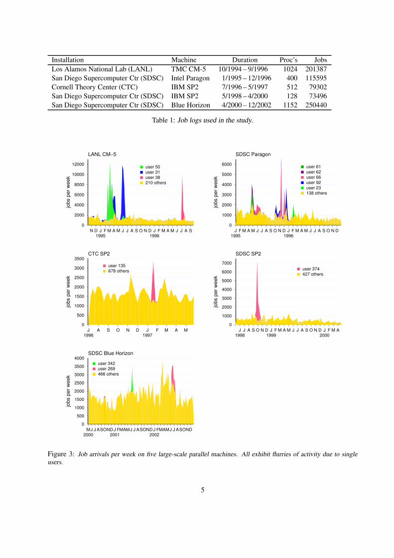
Installation Machine Duration Proc’s JobsLos Alamos National Lab (LANL) TMC CM-5 10/1994 – 9/1996 1024 201387San Diego Supercomputer Ctr (SDSC) Intel Paragon 1/1995 – 12/1996 400 115595Cornell Theory Center (CTC) IBM SP2 7/1996 – 5/1997 512 79302San Diego Supercomputer Ctr (SDSC) IBM SP2 5/1998 – 4/2000 128 73496San Diego Supercomputer Ctr (SDSC) Blue Horizon 4/2000 – 12/2002 1152 250440
Table 1: Job logs used in the study.
LANL CM−5
N D J1995
F M A M J J A S O N D J1996
F M A M J J A S
jobs
per
wee
k
0
2000
4000
6000
8000
10000
12000 user 50user 31user 38210 others
SDSC Paragon
J1995
F M A M J J A S O N D J1996
F M A M J J A S O N D
jobs
per
wee
k
0
1000
2000
3000
4000
5000
6000 user 61user 62user 66user 92user 23138 others
CTC SP2
J1996
A S O N D J1997
F M A M
jobs
per
wee
k
0
500
1000
1500
2000
2500
3000
3500
user 135678 others
SDSC SP2
J1998
J A S O N D J1999
F M A M J J A S O N D J2000
F M A
jobs
per
wee
k
0
1000
2000
3000
4000
5000
6000
7000user 374427 others
SDSC Blue Horizon
M2000
J J ASOND J2001
FMAMJ J ASOND J2002
FMAMJ J ASOND
jobs
per
wee
k
0
500
1000
1500
2000
2500
3000
3500
4000user 342user 269466 others
Figure 3: Job arrivals per week on five large-scale parallel machines. All exhibit flurries of activity due to singleusers.
5
SDSC SP2
J1998
J A S O N D J1999
F M A M J J A S O N D J2000
F M A
proc
esse
s pe
r wee
k (th
ousa
nds)
0
4
8
12
16
20user 21user 374user 197user 328423 others
SDSC Blue Horizon
M2000
J J ASOND J2001
FMAMJ J ASOND J2002
FMAMJ J ASOND
proc
esse
s pe
r wee
k (th
ousa
nds)
0
50
100
150
200
250
300user 68user 269466 others
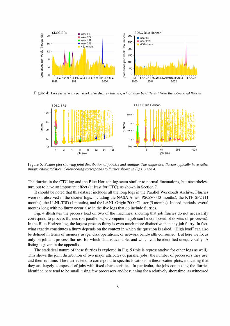
Figure 4: Process arrivals per week also display flurries, which may be different from the job-arrival flurries.
SDSC SP2
job size1 2 4 8 16 32 64 128
runt
ime
10s
1m
10m
1hr
10hr
SDSC Blue Horizon
job size16 64 256 1024
runt
ime
10s
1m
10m
1hr
10hr
Figure 5: Scatter plot showing joint distribution of job size and runtime. The single-user flurries typically have ratherunique characteristics. Color-coding corresponds to flurries shown in Figs. 3 and 4.
The flurries in the CTC log and the Blue Horizon log seem similar to normal fluctuations, but neverthelessturn out to have an important effect (at least for CTC), as shown in Section 7.
It should be noted that this dataset includes all the long logs in the Parallel Workloads Archive. Flurrieswere not observed in the shorter logs, including the NASA Ames iPSC/860 (3 months), the KTH SP2 (11months), the LLNL T3D (4 months), and the LANL Origin 2000 Cluster (5 months). Indeed, periods severalmonths long with no flurry occur also in the five logs that do include flurries.
Fig. 4 illustrates the process load on two of the machines, showing that job flurries do not necessarilycorrespond to process flurries (on parallel supercomputers a job can be composed of dozens of processes).In the Blue Horizon log, the largest process flurry is even much more distinctive than any job flurry. In fact,what exactly constitutes a flurry depends on the context in which the question is asked. “High load” can alsobe defined in terms of memory usage, disk operations, or network bandwidth consumed. But here we focusonly on job and process flurries, for which data is available, and which can be identified unequivocally. Alisting is given in the appendix.
The statistical nature of these flurries is explored in Fig. 5 (this is representative for other logs as well).This shows the joint distribution of two major attributes of parallel jobs: the number of processors they use,and their runtime. The flurries tend to correspond to specific locations in these scatter plots, indicating thatthey are largely composed of jobs with fixed characteristics. In particular, the jobs composing the flurriesidentified here tend to be small, using few processors and/or running for a relatively short time, as witnessed
6
CTC SP2
J1996
A S O N D J1997
F M A M
jobs
per
wee
k
0
500
1000
1500
2000
2500
3000
3500user 11user 135677 others
SDSC Paragon
J1995
F M A M J J A S O N D
jobs
per
wee
k
0
1000
2000
3000
4000
5000
6000 user 2user 5user 61user 92user 66136 others
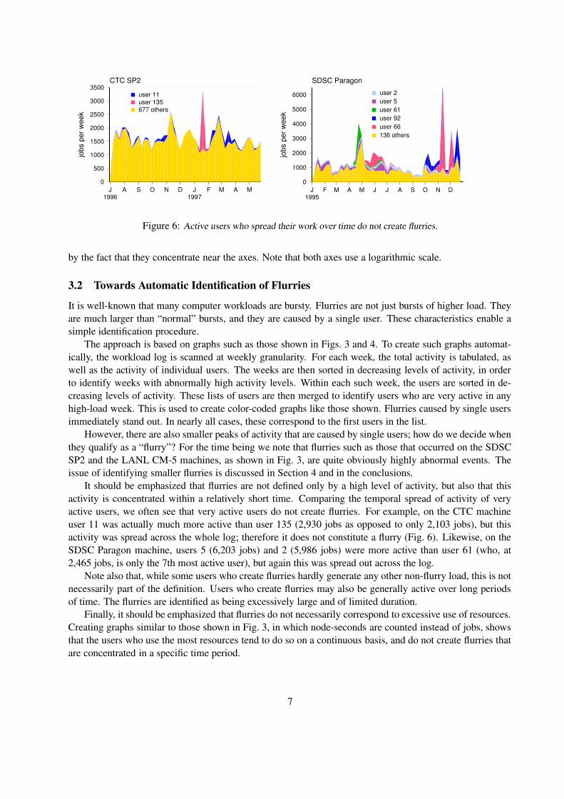
Figure 6: Active users who spread their work over time do not create flurries.
by the fact that they concentrate near the axes. Note that both axes use a logarithmic scale.
3.2 Towards Automatic Identification of Flurries
It is well-known that many computer workloads are bursty. Flurries are not just bursts of higher load. Theyare much larger than “normal” bursts, and they are caused by a single user. These characteristics enable asimple identification procedure.
The approach is based on graphs such as those shown in Figs. 3 and 4. To create such graphs automat-ically, the workload log is scanned at weekly granularity. For each week, the total activity is tabulated, aswell as the activity of individual users. The weeks are then sorted in decreasing levels of activity, in orderto identify weeks with abnormally high activity levels. Within each such week, the users are sorted in de-creasing levels of activity. These lists of users are then merged to identify users who are very active in anyhigh-load week. This is used to create color-coded graphs like those shown. Flurries caused by single usersimmediately stand out. In nearly all cases, these correspond to the first users in the list.
However, there are also smaller peaks of activity that are caused by single users; how do we decide whenthey qualify as a “flurry”? For the time being we note that flurries such as those that occurred on the SDSCSP2 and the LANL CM-5 machines, as shown in Fig. 3, are quite obviously highly abnormal events. Theissue of identifying smaller flurries is discussed in Section 4 and in the conclusions.
It should be emphasized that flurries are not defined only by a high level of activity, but also that thisactivity is concentrated within a relatively short time. Comparing the temporal spread of activity of veryactive users, we often see that very active users do not create flurries. For example, on the CTC machineuser 11 was actually much more active than user 135 (2,930 jobs as opposed to only 2,103 jobs), but thisactivity was spread across the whole log; therefore it does not constitute a flurry (Fig. 6). Likewise, on theSDSC Paragon machine, users 5 (6,203 jobs) and 2 (5,986 jobs) were more active than user 61 (who, at2,465 jobs, is only the 7th most active user), but again this was spread out across the log.
Note also that, while some users who create flurries hardly generate any other non-flurry load, this is notnecessarily part of the definition. Users who create flurries may also be generally active over long periodsof time. The flurries are identified as being excessively large and of limited duration.
Finally, it should be emphasized that flurries do not necessarily correspond to excessive use of resources.Creating graphs similar to those shown in Fig. 3, in which node-seconds are counted instead of jobs, showsthat the users who use the most resources tend to do so on a continuous basis, and do not create flurries thatare concentrated in a specific time period.
7
3.3 Related Work
Workload characterization and modeling have been advocated and practiced for many years [15, 7]. This istypically done by collecting workload traces, and creating a statistical model based on fitting the distributionsof workload attributes [19]. But such an approach is questionable if the data is not stationary, as seems to bethe case in the context of parallel supercomputers. For example, Chiang et al. analyze six non-consecutivemonths of data from the NCSA Origin 2000 machine, and find that the workloads in different months maybe quite different from each other [8]. We identify flurries as a specific type of deviations from stationaritythat have to be taken into account when creating a workload model.
Our notion of abnormal activity embodied by flurries seems complimentary to other work which had theopposite goal: to identify representative slices of the workload, in order to enable shorter but neverthelessreliable simulations. For example, in the context of evaluating computer architectures and cache designs,Lafage and Seznec suggest using short slices of applications [18], and Sherwood et al. suggest using basicblocks [29]. In both cases these are then clustered to find a small number of repeated segments that can rep-resent the whole application. This approach works due to the high regularity exhibited by typical computerprograms, which iterate among a limited number of computational phases.
In job-level workloads, on the other hand, the variability is much greater. As a result such clusteringcannot be fruitfully applied to the whole workload, but rather only to the activity of each user, leading tothe construction of a user behavior graph [14, 6]. While this can be used to construct a workload model thatreflects the variability introduced by different users, it cannot be used directly to identify abnormal behavior.However, it may be possible to use a second level of clustering, applied to the user behavior graphs, for thispurpose. At present we leave this idea for future work.
4 Flurries and Self-Similarity
Self similarity is the property of looking the same at different scales. In the context of workloads thistypically refers to different time scales, and implies that the workload is bursty at all granularities: it displayssmall bursts of activity at short time scales, and large swells of activity at long time scales. Such phenomenahave been seen in a wide variety of workloads, especially related to network traffic (see, e.g., [26]). It istherefore natural to ask whether flurries are just the largest in a whole spectrum of bursts of activity.
A well-known characteristic of self similarity is that the burstiness is retained when the process is ag-gregated, and viewed at a coarser time scale (this is in contradistinction from Poisson processes, where thefluctuations average out). The graphs shown in Figs. 3 and 4 are at the rather coarse granularity of a week.Indeed, they show a large degree of burstiness at this granularity. And importantly, this remains the case ifthe flurries are removed.
Self-similarity is quantified by the Hurst parameter H , which can be measured using Pox plots of theR/s (rescaled range) metric. Starting with a time series Xi specifying the number of arrivals in the ith timeunit, this is defined as [23, 27]
(
R
s
)
n
=maxj=1...n
∑ji=1
(Xi − X̄) − minj=1...n
∑ji=1
(Xi − X̄)√
1
n−1
∑ni=1
(Xi − X̄)2
The numerator measures the range of cumulative deviations from the mean, and the denominator rescalesthis range by the standard deviation. To create a Pox plot, this is repeated for subsequences of differentlengths n, and moreover different subsequences for each n (that is, not only the first n, but also the subse-quence from n + 1 to 2n, etc.), and the results plotted in a scatter plot on log-log axes. Self similarity ismanifested by a linear relationship, with the slope of the regression line giving the Hurst parameter, whichshould lie in the range 1
2< H < 1.
8
Jobs (original with flurries)
n16 64 256 1K 4K 16K 64K 256K
R/s
8
32
128
512
2048
8192
H=0.781R^2=0.976
user 21user 374user 197user 328others
Processes (original with flurries)
n16 64 256 1K 4K 16K 64K 256K
R/s
8
32
128
512
2048
8192
H=0.662R^2=0.973
user 21user 374user 197user 328others
Jobs (flurries removed)
n16 64 256 1K 4K 16K 64K 256K
R/s
8
32
128
512
2048
8192
H=0.695R^2=0.986
Processes (flurries removed)
n16 64 256 1K 4K 16K 64K 256K
R/s
8
32
128
512
2048
8192
H=0.689R^2=0.985
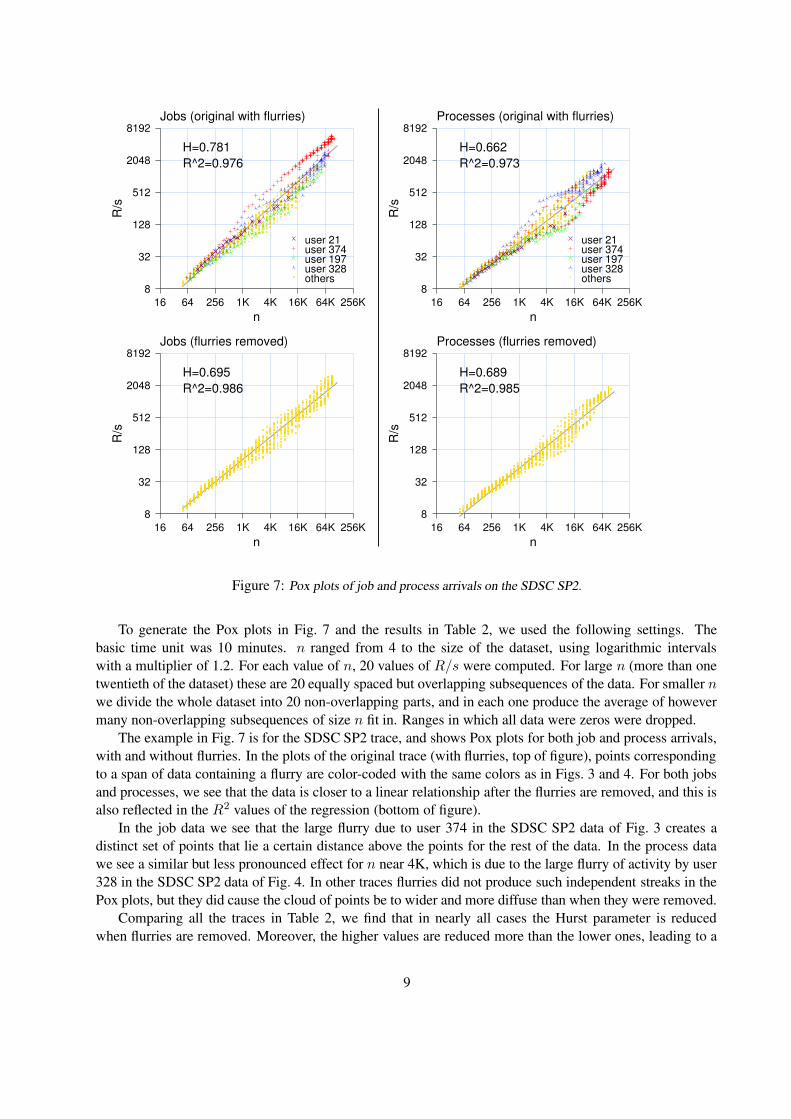
Figure 7: Pox plots of job and process arrivals on the SDSC SP2.
To generate the Pox plots in Fig. 7 and the results in Table 2, we used the following settings. Thebasic time unit was 10 minutes. n ranged from 4 to the size of the dataset, using logarithmic intervalswith a multiplier of 1.2. For each value of n, 20 values of R/s were computed. For large n (more than onetwentieth of the dataset) these are 20 equally spaced but overlapping subsequences of the data. For smaller nwe divide the whole dataset into 20 non-overlapping parts, and in each one produce the average of howevermany non-overlapping subsequences of size n fit in. Ranges in which all data were zeros were dropped.
The example in Fig. 7 is for the SDSC SP2 trace, and shows Pox plots for both job and process arrivals,with and without flurries. In the plots of the original trace (with flurries, top of figure), points correspondingto a span of data containing a flurry are color-coded with the same colors as in Figs. 3 and 4. For both jobsand processes, we see that the data is closer to a linear relationship after the flurries are removed, and this isalso reflected in the R2 values of the regression (bottom of figure).
In the job data we see that the large flurry due to user 374 in the SDSC SP2 data of Fig. 3 creates adistinct set of points that lie a certain distance above the points for the rest of the data. In the process datawe see a similar but less pronounced effect for n near 4K, which is due to the large flurry of activity by user328 in the SDSC SP2 data of Fig. 4. In other traces flurries did not produce such independent streaks in thePox plots, but they did cause the cloud of points be to wider and more diffuse than when they were removed.
Comparing all the traces in Table 2, we find that in nearly all cases the Hurst parameter is reducedwhen flurries are removed. Moreover, the higher values are reduced more than the lower ones, leading to a
9
jobs processestrace original cleaned original cleanedLANL CM-5 0.844 (0.969) 0.771 (0.975) 0.832 (0.969) 0.740 (0.973)SDSC Paragon 0.822 (0.981) 0.764 (0.986) 0.742 (0.980) 0.673 (0.982)CTC SP2 0.657 (0.981) 0.646 (0.980) 0.653 (0.991) 0.656 (0.991)SDSC SP2 0.781 (0.976) 0.695 (0.986) 0.662 (0.973) 0.689 (0.985)SDSC Blue H. 0.781 (0.986) 0.765 (0.986) 0.716 (0.985) 0.694 (0.988)
Table 2: Changes to the Hurst parameter of job and process arrivals to supercomputers when the flurries are removed.Note that the range of values observed in different logs is reduced, leading to greater consistency. R2 values are givenin parentheses; they also tend to improve when flurries are removed.
concentration of the different values in a somewhat narrower range. In addition, the R2 values either staythe same or are improved when flurries are removed. Nevertheless, removing the flurries does not cause asignificant qualitative difference to the Pox plots or H values.
Thus, while flurries make a certain contribution to the detection and quantification of self similarity,they are not crucial for it. Moreover, flurries are different from self-similarity in two ways. First, someof the flurries are large bursts of activity that occur over short time scales, on a background of relativelystable normal activity. Indeed, the activity graphs shown in Fig. 3, while showing bursts of activity, are quitedifferent from the graphs showing bursts at different time scales typically used to illustrate self similarity(e.g. [20, 31]). Second, in the context of network traffic, self-similarity only refers to the arrival process, i.e.to the temporal structure of the workload. In flurries we also include the repetitive nature of the jobs (size,runtimes, etc.), which leads to modal distributions of workload parameters as demonstrated below.
In interpreting these results, it is important to note that many users commonly display activity patternsin which a lot of repetitive work is concentrated in a short time span. These bursts of activity cover a wholespectrum of sizes, from very small to rather significant. The question is then whether flurries are just thelargest in a continuum of effects. In our opinion, the large job flurries like those observed on the LANLCM5 and the SDSC SP2 machines are truly exceptional, and are so much larger than any other event thatthey certainly qualify as a distinct type of phenomenon. But the job flurries on the CTC SP2 and SDSCBlue Horizon, and most of the process flurries on the SDSC SP2, may be just the largest of a continuum.Nevertheless, they may still have an uncomfortably large impact on modeling and evaluation results, asshown in the following sections. This justifies the idea of separate evaluations, with the flurries and withoutthem.
5 The Effect of Flurries on Workload Modeling
Workload modeling attempts to generalize from specific workloads by finding invariants that are commonto workloads from similar settings [4]. Workload flurries interfere with this endeavor by their obvious effecton workload statistics. By definition, a flurry involves a large number of similar jobs. The combined weightof these jobs can cause significant modifications to the distributions of various workload parameters relativeto the background load in which no flurries are present.
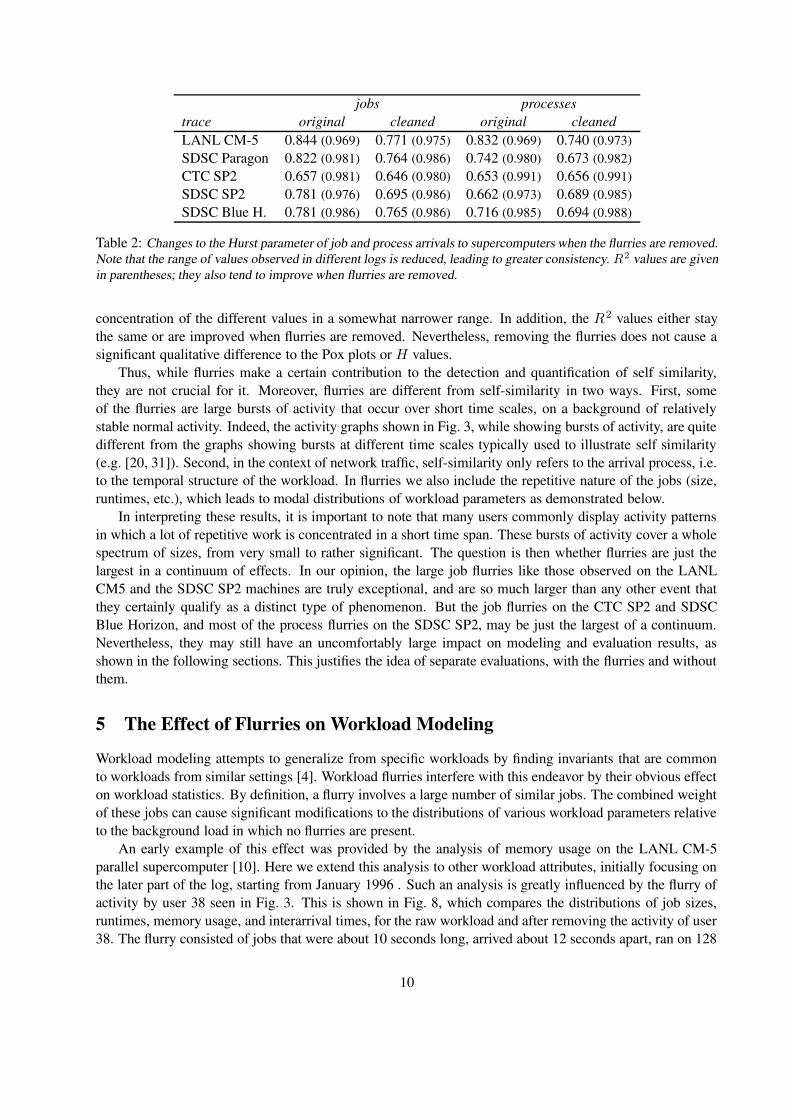
An early example of this effect was provided by the analysis of memory usage on the LANL CM-5parallel supercomputer [10]. Here we extend this analysis to other workload attributes, initially focusing onthe later part of the log, starting from January 1996 . Such an analysis is greatly influenced by the flurry ofactivity by user 38 seen in Fig. 3. This is shown in Fig. 8, which compares the distributions of job sizes,runtimes, memory usage, and interarrival times, for the raw workload and after removing the activity of user38. The flurry consisted of jobs that were about 10 seconds long, arrived about 12 seconds apart, ran on 128
10
job size32 128 512
cum
ulat
ive
% jo
bs
0
0.2
0.4
0.6
0.8
1
all jobs ’95w/o fluries ’95all jobs ’96w/o flurries ’96
job runtime [s]10s 1m 10m 1hr 10hr
cum
ulat
ive
% jo
bs
0
0.2
0.4
0.6
0.8
1
memory per node [MB]0.25 1 4 16
cum
ulat
ive
% jo
bs
0
0.2
0.4
0.6
0.8
1
interarrival time [s]1s 30s 5m 1hr
cum
ulat
ive
% jo
bs
0
0.2
0.4
0.6
0.8
1
Figure 8: Changes to the distributions of workload attributes when flurries are removed from the LANL CM-5 log.Most differences between 1995 and 1996 may be attributed to the different flurries.
nodes, and used either very little memory or about 1.84 MB per node. This accounted for 12,344 (29%) ofthe total of 42,702 jobs in this part of the log.
For comparison, we repeated this exercise using the 1995 portion of the log, which contains two flurriesby users 31 and 50. There were a total of 123,058 jobs in that year, of which an amazing 71,161 (58%)belonged to the two rather large flurries. Fig. 8 also shows the 1995 results. It immediately shows thatthe distributions of the cleaned logs in the two years are pretty similar to each other (solid lines), whereasthe distributions of the raw logs are quite distinct (dashed lines), due to the modifications caused by thedifferent flurries. This is an extremely important result, as it implies that the base workload (without theflurries) is actually quite consistent across a long period of time, suggesting that the data is stationary. Themajor differences between 1995 and 1996 are actually the result of flurries introduced by 3 users out of atotal population of 213. As may be expected, the modifications caused by the flurries are both qualitative andquantitative: the distributions become more modal, and emphasize shorter runtimes and interarrival times.
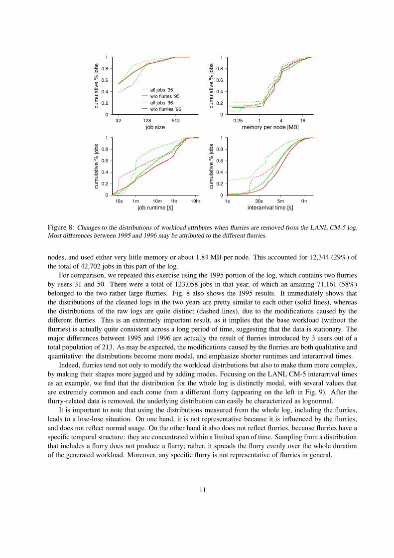
Indeed, flurries tend not only to modify the workload distributions but also to make them more complex,by making their shapes more jagged and by adding modes. Focusing on the LANL CM-5 interarrival timesas an example, we find that the distribution for the whole log is distinctly modal, with several values thatare extremely common and each come from a different flurry (appearing on the left in Fig. 9). After theflurry-related data is removed, the underlying distribution can easily be characterized as lognormal.
It is important to note that using the distributions measured from the whole log, including the flurries,leads to a lose-lose situation. On one hand, it is not representative because it is influenced by the flurries,and does not reflect normal usage. On the other hand it also does not reflect flurries, because flurries have aspecific temporal structure: they are concentrated within a limited span of time. Sampling from a distributionthat includes a flurry does not produce a flurry; rather, it spreads the flurry evenly over the whole durationof the generated workload. Moreover, any specific flurry is not representative of flurries in general.
11
interarrival time1s 10s 1m 10m 1hr 10hr
num
ber o
f job
s
0
2000
4000
6000
8000
24490 15124
base distrib.additions dueto flurries
Figure 9: Flurries turn the lognormal distribution of interarrival times into a noisy and modal distribution. Data fromLANL CM-5.
6 The Effect of Flurries on Performance Evaluation: A Case Studyof Instability
Apart from the effect flurries have on workload statistics, and through them on workload modeling, theyalso may have a significant effect on performance evaluation results. In this section we will present a casestudy showing how the presence of a flurry leads to unstable results: very small changes to the workload areamplified by the flurry and lead to an unexpectedly large change in the results. The next section will furtherdemonstrate that such effects indeed cause problems in practice.
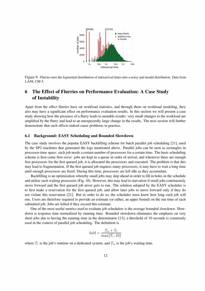
6.1 Background: EASY Scheduling and Bounded Slowdown
The case study involves the popular EASY backfilling scheme for batch parallel job scheduling [21], usedby the SP2 machines that generated the logs mentioned above. Parallel jobs can be seen as rectangles inprocessor-time space: each job needs a certain number of processors for a certain time. The basic schedulingscheme is first-come first-serve: jobs are kept in a queue in order of arrival, and whenever there are enoughfree processors for the first queued job, it is allocated the processors and executed. The problem is that thismay lead to fragmentation. If the first queued job requires many processors, it may have to wait a long timeuntil enough processors are freed. During this time, processors are left idle as they accumulate.
Backfilling is an optimization whereby small jobs may skip ahead in order to fill in holes in the scheduleand utilize such waiting processors (Fig. 10). However, this may lead to starvation if small jobs continuouslymove forward and the first queued job never gets to run. The solution adopted by the EASY scheduler isto first make a reservation for the first queued job, and allow later jobs to move forward only if they donot violate this reservation [21]. But in order to do so, the scheduler must know how long each job willrun. Users are therefore required to provide an estimate (or rather, an upper bound) on the run time of eachsubmitted job. Jobs are killed if they exceed this estimate.
One of the most useful metrics used to evaluate job schedulers is the average bounded slowdown. Slow-down is response time normalized by running time. Bounded slowdown eliminates the emphasis on veryshort jobs due to having the running time in the denominator [13]; a threshold of 10 seconds is commonlyused in the context of parallel job scheduling. The definition is
bsld =Tw + Tr
max{Tr, 10}
where Tr is the job’s runtime on a dedicated system, and Tw is the job’s waiting time.
12
TimeTime
FCFS
Nod
es
EASY
Nod
es
43
43
2
1
2
1
Figure 10: Left: FCFS scheduling (jobs numbered in order of arrival). Right: FCFS with backfilling. Note that itwould be impossible to backfill job 4 had its length been more than 2, as the reservation for job 3 would have beenviolated.
81
82
83
84
85
86
87
88
89
-300 -200 -100 0 100 200 300
avg.
bou
nded
slo
wdo
wn
offset from original runtime [sec]
Figure 11: Average bounded slowdown obtained by the EASY scheduler on the SDSC trace, as a function of changingthe runtime of job 59,210.
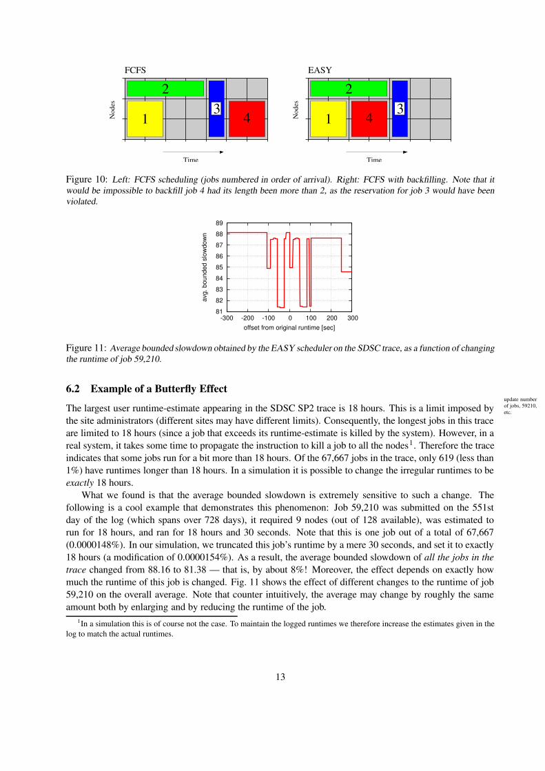
6.2 Example of a Butterfly Effectupdate numberof jobs, 59210,etc.The largest user runtime-estimate appearing in the SDSC SP2 trace is 18 hours. This is a limit imposed by
the site administrators (different sites may have different limits). Consequently, the longest jobs in this traceare limited to 18 hours (since a job that exceeds its runtime-estimate is killed by the system). However, in areal system, it takes some time to propagate the instruction to kill a job to all the nodes1. Therefore the traceindicates that some jobs run for a bit more than 18 hours. Of the 67,667 jobs in the trace, only 619 (less than1%) have runtimes longer than 18 hours. In a simulation it is possible to change the irregular runtimes to beexactly 18 hours.
What we found is that the average bounded slowdown is extremely sensitive to such a change. Thefollowing is a cool example that demonstrates this phenomenon: Job 59,210 was submitted on the 551stday of the log (which spans over 728 days), it required 9 nodes (out of 128 available), was estimated torun for 18 hours, and ran for 18 hours and 30 seconds. Note that this is one job out of a total of 67,667(0.0000148%). In our simulation, we truncated this job’s runtime by a mere 30 seconds, and set it to exactly18 hours (a modification of 0.0000154%). As a result, the average bounded slowdown of all the jobs in thetrace changed from 88.16 to 81.38 — that is, by about 8%! Moreover, the effect depends on exactly howmuch the runtime of this job is changed. Fig. 11 shows the effect of different changes to the runtime of job59,210 on the overall average. Note that counter intuitively, the average may change by roughly the sameamount both by enlarging and by reducing the runtime of the job.
1In a simulation this is of course not the case. To maintain the logged runtimes we therefore increase the estimates given in thelog to match the actual runtimes.
13
-60
-40
-20
0
20
40
60
550 555 560 565 570 575 580 585
star
t-tim
e di
ffere
nce
[hou
rs]
job submission time [days]
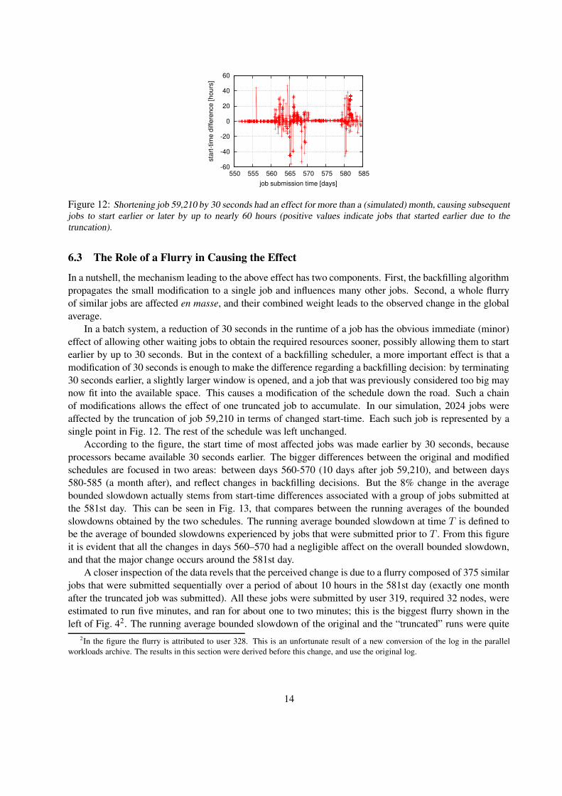
Figure 12: Shortening job 59,210 by 30 seconds had an effect for more than a (simulated) month, causing subsequentjobs to start earlier or later by up to nearly 60 hours (positive values indicate jobs that started earlier due to thetruncation).
6.3 The Role of a Flurry in Causing the Effect
In a nutshell, the mechanism leading to the above effect has two components. First, the backfilling algorithmpropagates the small modification to a single job and influences many other jobs. Second, a whole flurryof similar jobs are affected en masse, and their combined weight leads to the observed change in the globalaverage.
In a batch system, a reduction of 30 seconds in the runtime of a job has the obvious immediate (minor)effect of allowing other waiting jobs to obtain the required resources sooner, possibly allowing them to startearlier by up to 30 seconds. But in the context of a backfilling scheduler, a more important effect is that amodification of 30 seconds is enough to make the difference regarding a backfilling decision: by terminating30 seconds earlier, a slightly larger window is opened, and a job that was previously considered too big maynow fit into the available space. This causes a modification of the schedule down the road. Such a chainof modifications allows the effect of one truncated job to accumulate. In our simulation, 2024 jobs wereaffected by the truncation of job 59,210 in terms of changed start-time. Each such job is represented by asingle point in Fig. 12. The rest of the schedule was left unchanged.
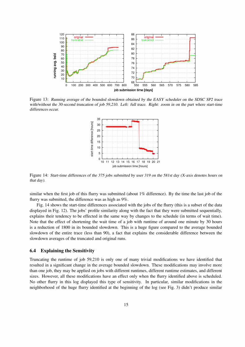
According to the figure, the start time of most affected jobs was made earlier by 30 seconds, becauseprocessors became available 30 seconds earlier. The bigger differences between the original and modifiedschedules are focused in two areas: between days 560-570 (10 days after job 59,210), and between days580-585 (a month after), and reflect changes in backfilling decisions. But the 8% change in the averagebounded slowdown actually stems from start-time differences associated with a group of jobs submitted atthe 581st day. This can be seen in Fig. 13, that compares between the running averages of the boundedslowdowns obtained by the two schedules. The running average bounded slowdown at time T is defined tobe the average of bounded slowdowns experienced by jobs that were submitted prior to T . From this figureit is evident that all the changes in days 560–570 had a negligible affect on the overall bounded slowdown,and that the major change occurs around the 581st day.
A closer inspection of the data revels that the perceived change is due to a flurry composed of 375 similarjobs that were submitted sequentially over a period of about 10 hours in the 581st day (exactly one monthafter the truncated job was submitted). All these jobs were submitted by user 319, required 32 nodes, wereestimated to run five minutes, and ran for about one to two minutes; this is the biggest flurry shown in theleft of Fig. 42. The running average bounded slowdown of the original and the “truncated” runs were quite
2In the figure the flurry is attributed to user 328. This is an unfortunate result of a new conversion of the log in the parallelworkloads archive. The results in this section were derived before this change, and use the original log.
14
10 20 30 40 50 60 70 80 90
100 110 120
0 100 200 300 400 500 600 700 800
runn
ing
avg.
bsl
d
job submission time [days]
originaltruncated
68
70
72
74
76
78
80
82
84
86
88
550 555 560 565 570 575 580 585
runn
ing
avg.
bsl
d
job submission time [days]
originaltruncated
Figure 13: Running average of the bounded slowdown obtained by the EASY scheduler on the SDSC SP2 tracewith/without the 30-second truncation of job 59,210. Left: full trace. Right: zoom in on the part where start-timedifferences occur.
0
5
10
15
20
25
30
35
10 11 12 13 14 15 16 17 18 19 20 21
star
t-tim
e di
ffere
nce
[hou
rs]
job submission time [hours]
Figure 14: Start-time differences of the 375 jobs submitted by user 319 on the 581st day (X-axis denotes hours onthat day).
similar when the first job of this flurry was submitted (about 1% difference). By the time the last job of theflurry was submitted, the difference was as high as 9%.
Fig. 14 shows the start-time differences associated with the jobs of the flurry (this is a subset of the datadisplayed in Fig. 12). The jobs’ profile similarity along with the fact that they were submitted sequentially,explains their tendency to be effected in the same way by changes to the schedule (in terms of wait time).Note that the effect of shortening the wait time of a job with runtime of around one minute by 30 hoursis a reduction of 1800 in its bounded slowdown. This is a huge figure compared to the average boundedslowdown of the entire trace (less than 90), a fact that explains the considerable difference between theslowdown averages of the truncated and original runs.
6.4 Explaining the Sensitivity
Truncating the runtime of job 59,210 is only one of many trivial modifications we have identified thatresulted in a significant change in the average bounded slowdown. These modifications may involve morethan one job, they may be applied on jobs with different runtimes, different runtime estimates, and differentsizes. However, all these modifications have an effect only when the flurry identified above is scheduled.No other flurry in this log displayed this type of sensitivity. In particular, similar modifications in theneighborhood of the huge flurry identified at the beginning of the log (see Fig. 3) didn’t produce similar
15
0
5
10
15
20
25
0 100 200 300 400 500 600 700 800
proc
ess
load
time [days]
weekly avg.running avg.
0 10 20 30 40 50 60 70 80 90
0 100 200 300 400 500 600 700 800
wai
t-que
ue le
ngth
time [days]
weekly avg.running avg.
Figure 15: Evolution of the SDSC SP2 process load and the waiting-queue length when simulating EASY on theoriginal trace.
effects, even though the earlier flurry is an order of magnitude bigger than the later one (in terms of thenumber of jobs composing it).
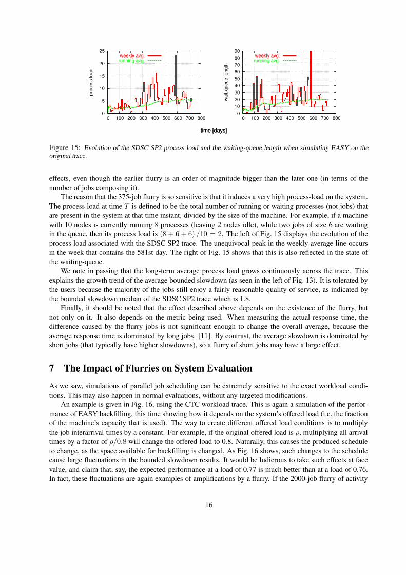
The reason that the 375-job flurry is so sensitive is that it induces a very high process-load on the system.The process load at time T is defined to be the total number of running or waiting processes (not jobs) thatare present in the system at that time instant, divided by the size of the machine. For example, if a machinewith 10 nodes is currently running 8 processes (leaving 2 nodes idle), while two jobs of size 6 are waitingin the queue, then its process load is (8 + 6 + 6) /10 = 2. The left of Fig. 15 displays the evolution of theprocess load associated with the SDSC SP2 trace. The unequivocal peak in the weekly-average line occursin the week that contains the 581st day. The right of Fig. 15 shows that this is also reflected in the state ofthe waiting-queue.
We note in passing that the long-term average process load grows continuously across the trace. Thisexplains the growth trend of the average bounded slowdown (as seen in the left of Fig. 13). It is tolerated bythe users because the majority of the jobs still enjoy a fairly reasonable quality of service, as indicated bythe bounded slowdown median of the SDSC SP2 trace which is 1.8.
Finally, it should be noted that the effect described above depends on the existence of the flurry, butnot only on it. It also depends on the metric being used. When measuring the actual response time, thedifference caused by the flurry jobs is not significant enough to change the overall average, because theaverage response time is dominated by long jobs. [11]. By contrast, the average slowdown is dominated byshort jobs (that typically have higher slowdowns), so a flurry of short jobs may have a large effect.
7 The Impact of Flurries on System Evaluation
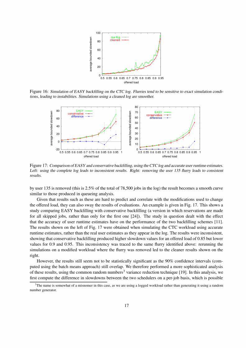
As we saw, simulations of parallel job scheduling can be extremely sensitive to the exact workload condi-tions. This may also happen in normal evaluations, without any targeted modifications.
An example is given in Fig. 16, using the CTC workload trace. This is again a simulation of the perfor-mance of EASY backfilling, this time showing how it depends on the system’s offered load (i.e. the fractionof the machine’s capacity that is used). The way to create different offered load conditions is to multiplythe job interarrival times by a constant. For example, if the original offered load is ρ, multiplying all arrivaltimes by a factor of ρ/0.8 will change the offered load to 0.8. Naturally, this causes the produced scheduleto change, as the space available for backfilling is changed. As Fig. 16 shows, such changes to the schedulecause large fluctuations in the bounded slowdown results. It would be ludicrous to take such effects at facevalue, and claim that, say, the expected performance at a load of 0.77 is much better than at a load of 0.76.In fact, these fluctuations are again examples of amplifications by a flurry. If the 2000-job flurry of activity
16
0
20
40
60
80
100
0.5 0.55 0.6 0.65 0.7 0.75 0.8 0.85 0.9 0.95
aver
age
boun
ded
slow
dow
n
offered load
raw logcleaned
Figure 16: Simulation of EASY backfilling on the CTC log. Flurries tend to be sensitive to exact simulation condi-tions, leading to instabilities. Simulations using a cleaned log are smoother.
-20
0
20
40
60
80
0.5 0.55 0.6 0.65 0.7 0.75 0.8 0.85 0.9 0.95 1
aver
age
boun
ded
slow
dow
n
offered load
EASYconservative
difference
0
10
20
30
40
50
60
70
80
0.5 0.55 0.6 0.65 0.7 0.75 0.8 0.85 0.9 0.95 1
aver
age
boun
ded
slow
dow
n
offered load
EASYconservative
difference
Figure 17: Comparison of EASY and conservative backfilling, using the CTC log and accurate user runtime estimates.Left: using the complete log leads to inconsistent results. Right: removing the user 135 flurry leads to consistentresults.
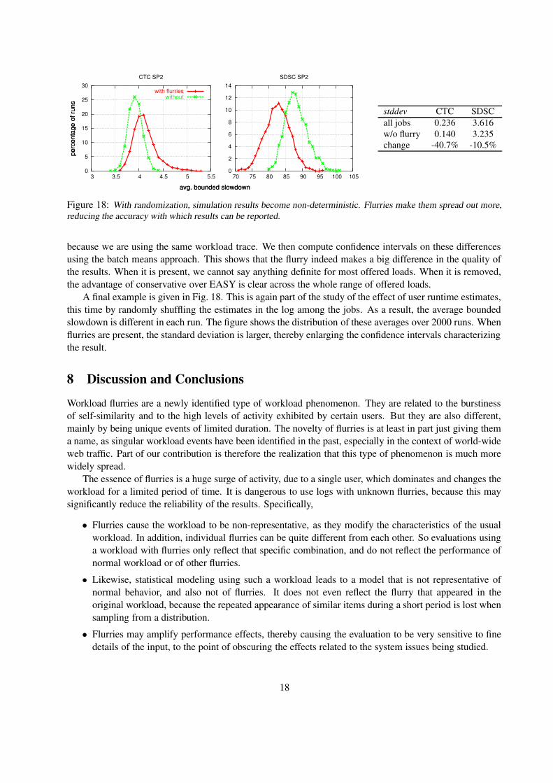
by user 135 is removed (this is 2.5% of the total of 78,500 jobs in the log) the result becomes a smooth curvesimilar to those produced in queueing analysis.
Given that results such as these are hard to predict and correlate with the modifications used to changethe offered load, they can also sway the results of evaluations. An example is given in Fig. 17. This shows astudy comparing EASY backfilling with conservative backfilling (a version in which reservations are madefor all skipped jobs, rather than only for the first one [24]). The study in question dealt with the effectthat the accuracy of user runtime estimates have on the performance of the two backfilling schemes [11].The results shown on the left of Fig. 17 were obtained when simulating the CTC workload using accurateruntime estimates, rather than the real user estimates as they appear in the log. The results were inconsistent,showing that conservative backfilling produced higher slowdown values for an offered load of 0.85 but lowervalues for 0.9 and 0.95. This inconsistency was traced to the same flurry identified above: rerunning thesimulations on a modified workload where the flurry was removed led to the cleaner results shown on theright.
However, the results still seem not to be statistically significant as the 90% confidence intervals (com-puted using the batch means approach) still overlap. We therefore performed a more sophisticated analysisof these results, using the common random numbers3 variance reduction technique [19]. In this analysis, wefirst compute the difference in slowdowns between the two schedulers on a per-job basis, which is possible
3The name is somewhat of a misnomer in this case, as we are using a logged workload rather than generating it using a randomnumber generator.
17
0
5
10
15
20
25
30
3 3.5 4 4.5 5 5.5
CTC SP2pe
rcen
tage
of r
uns
avg. bounded slowdown
with flurrieswithout
0
2
4
6
8
10
12
14
70 75 80 85 90 95 100 105
SDSC SP2pe
rcen
tage
of r
uns
avg. bounded slowdown
stddev CTC SDSCall jobs 0.236 3.616w/o flurry 0.140 3.235change -40.7% -10.5%
Figure 18: With randomization, simulation results become non-deterministic. Flurries make them spread out more,reducing the accuracy with which results can be reported.
because we are using the same workload trace. We then compute confidence intervals on these differencesusing the batch means approach. This shows that the flurry indeed makes a big difference in the quality ofthe results. When it is present, we cannot say anything definite for most offered loads. When it is removed,the advantage of conservative over EASY is clear across the whole range of offered loads.
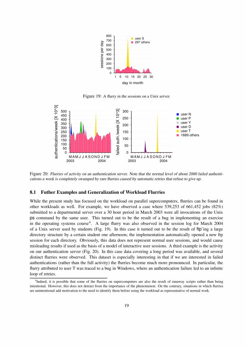
A final example is given in Fig. 18. This is again part of the study of the effect of user runtime estimates,this time by randomly shuffling the estimates in the log among the jobs. As a result, the average boundedslowdown is different in each run. The figure shows the distribution of these averages over 2000 runs. Whenflurries are present, the standard deviation is larger, thereby enlarging the confidence intervals characterizingthe result.
8 Discussion and Conclusions
Workload flurries are a newly identified type of workload phenomenon. They are related to the burstinessof self-similarity and to the high levels of activity exhibited by certain users. But they are also different,mainly by being unique events of limited duration. The novelty of flurries is at least in part just giving thema name, as singular workload events have been identified in the past, especially in the context of world-wideweb traffic. Part of our contribution is therefore the realization that this type of phenomenon is much morewidely spread.
The essence of flurries is a huge surge of activity, due to a single user, which dominates and changes theworkload for a limited period of time. It is dangerous to use logs with unknown flurries, because this maysignificantly reduce the reliability of the results. Specifically,
• Flurries cause the workload to be non-representative, as they modify the characteristics of the usualworkload. In addition, individual flurries can be quite different from each other. So evaluations usinga workload with flurries only reflect that specific combination, and do not reflect the performance ofnormal workload or of other flurries.
• Likewise, statistical modeling using such a workload leads to a model that is not representative ofnormal behavior, and also not of flurries. It does not even reflect the flurry that appeared in theoriginal workload, because the repeated appearance of similar items during a short period is lost whensampling from a distribution.
• Flurries may amplify performance effects, thereby causing the evaluation to be very sensitive to finedetails of the input, to the point of obscuring the effects related to the system issues being studied.
18
day in month
1 5 10 15 20 25 30
sess
ions
per
day
0100200300400500600700800
user S297 others
Figure 19: A flurry in the sessions on a Unix server.
M2003
AM J J A S O N D J2004
FMauth
entic
atio
ns/w
eek
[X 1
0^3]
050
100150200250300350400450500
user Nuser Puser Yuser Duser T1689 others
M2003
AM J J A S O N D J2004
FM
faile
d au
th./w
eek
[X 1
0^3]
0
50
100
150
200
250
300
Figure 20: Flurries of activity on an authentication server. Note that the normal level of about 2000 failed authenti-cations a week is completely swamped by rare flurries caused by automatic retries that refuse to give up.
8.1 Futher Examples and Generalization of Workload Flurries
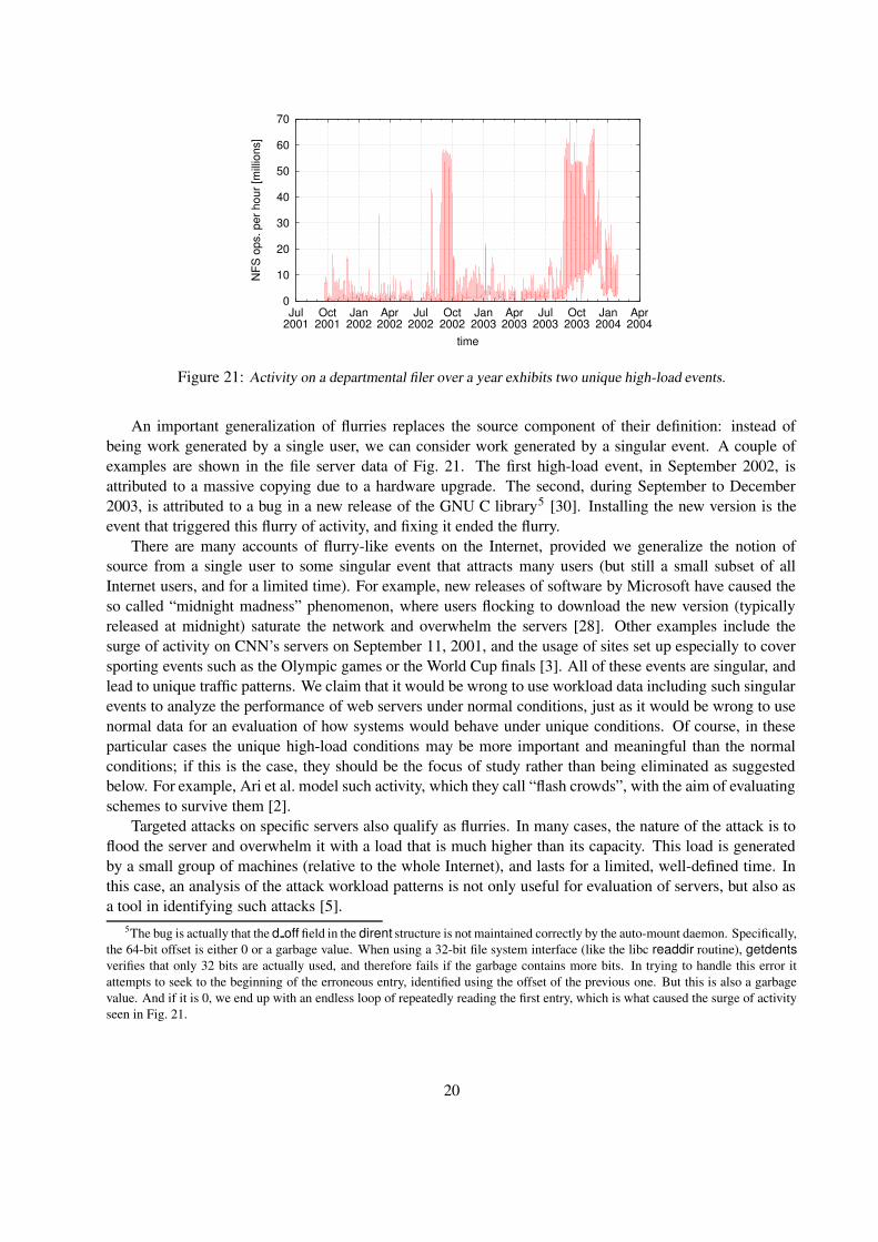
While the present study has focused on the workload on parallel supercomputers, flurries can be found inother workloads as well. For example, we have observed a case where 539,253 of 661,452 jobs (82%)submitted to a departmental server over a 30 hour period in March 2003 were all invocations of the Unixps command by the same user. This turned out to be the result of a bug in implementing an exercisein the operating systems course4. A large flurry was also observed in the session log for March 2004of a Unix server used by students (Fig. 19). In this case it turned out to be the result of ftp’ing a largedirectory structure by a certain student one afternoon; the implementation automatically opened a new ftpsession for each directory. Obviously, this data does not represent normal user sessions, and would causemisleading results if used as the basis of a model of interactive user sessions. A third example is the activityon our authentication server (Fig. 20). In this case data covering a long period was available, and severaldistinct flurries were observed. This dataset is especially interesting in that if we are interested in failedauthentications (rather than the full activity) the flurries become much more pronounced. In particular, theflurry attributed to user T was traced to a bug in Windows, where an authentication failure led to an infiniteloop of retries.
4Indeed, it is possible that some of the flurries on supercomputers are also the result of runaway scripts rather than beingintentional. However, this does not detract from the importance of the phenomenon. On the contrary, situations in which flurriesare unintentional add motivation to the need to identify them before using the workload as representative of normal work.
19
0
10
20
30
40
50
60
70
Jul2001
Oct2001
Jan2002
Apr2002
Jul2002
Oct2002
Jan2003
Apr2003
Jul2003
Oct2003
Jan2004
Apr2004
NFS
ops
. per
hou
r [m
illio
ns]
time
Figure 21: Activity on a departmental filer over a year exhibits two unique high-load events.
An important generalization of flurries replaces the source component of their definition: instead ofbeing work generated by a single user, we can consider work generated by a singular event. A couple ofexamples are shown in the file server data of Fig. 21. The first high-load event, in September 2002, isattributed to a massive copying due to a hardware upgrade. The second, during September to December2003, is attributed to a bug in a new release of the GNU C library5 [30]. Installing the new version is theevent that triggered this flurry of activity, and fixing it ended the flurry.
There are many accounts of flurry-like events on the Internet, provided we generalize the notion ofsource from a single user to some singular event that attracts many users (but still a small subset of allInternet users, and for a limited time). For example, new releases of software by Microsoft have caused theso called “midnight madness” phenomenon, where users flocking to download the new version (typicallyreleased at midnight) saturate the network and overwhelm the servers [28]. Other examples include thesurge of activity on CNN’s servers on September 11, 2001, and the usage of sites set up especially to coversporting events such as the Olympic games or the World Cup finals [3]. All of these events are singular, andlead to unique traffic patterns. We claim that it would be wrong to use workload data including such singularevents to analyze the performance of web servers under normal conditions, just as it would be wrong to usenormal data for an evaluation of how systems would behave under unique conditions. Of course, in theseparticular cases the unique high-load conditions may be more important and meaningful than the normalconditions; if this is the case, they should be the focus of study rather than being eliminated as suggestedbelow. For example, Ari et al. model such activity, which they call “flash crowds”, with the aim of evaluatingschemes to survive them [2].
Targeted attacks on specific servers also qualify as flurries. In many cases, the nature of the attack is toflood the server and overwhelm it with a load that is much higher than its capacity. This load is generatedby a small group of machines (relative to the whole Internet), and lasts for a limited, well-defined time. Inthis case, an analysis of the attack workload patterns is not only useful for evaluation of servers, but also asa tool in identifying such attacks [5].
5The bug is actually that the d off field in the dirent structure is not maintained correctly by the auto-mount daemon. Specifically,the 64-bit offset is either 0 or a garbage value. When using a 32-bit file system interface (like the libc readdir routine), getdentsverifies that only 32 bits are actually used, and therefore fails if the garbage contains more bits. In trying to handle this error itattempts to seek to the beginning of the erroneous entry, identified using the offset of the previous one. But this is also a garbagevalue. And if it is 0, we end up with an endless loop of repeatedly reading the first entry, which is what caused the surge of activityseen in Fig. 21.
20
8.2 Dealing with Flurries
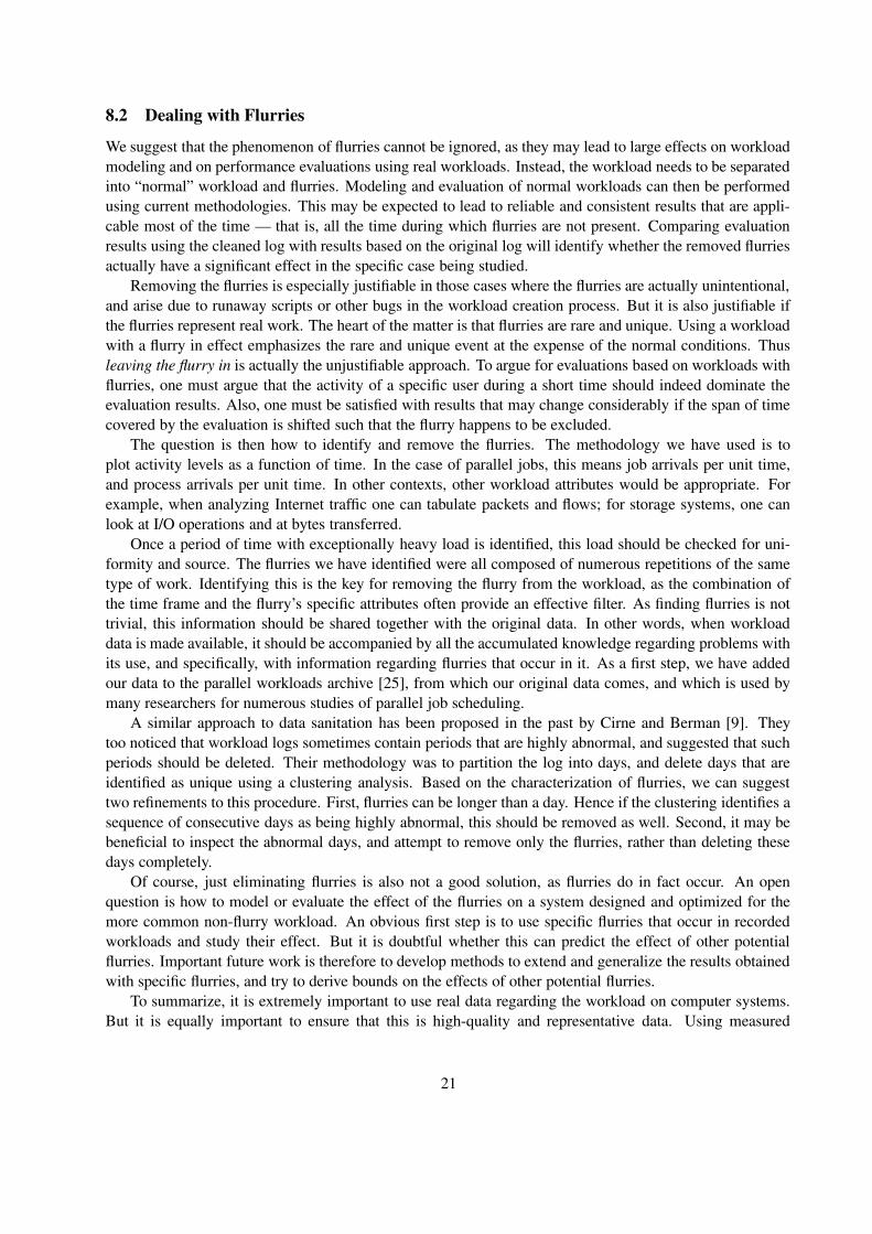
We suggest that the phenomenon of flurries cannot be ignored, as they may lead to large effects on workloadmodeling and on performance evaluations using real workloads. Instead, the workload needs to be separatedinto “normal” workload and flurries. Modeling and evaluation of normal workloads can then be performedusing current methodologies. This may be expected to lead to reliable and consistent results that are appli-cable most of the time — that is, all the time during which flurries are not present. Comparing evaluationresults using the cleaned log with results based on the original log will identify whether the removed flurriesactually have a significant effect in the specific case being studied.
Removing the flurries is especially justifiable in those cases where the flurries are actually unintentional,and arise due to runaway scripts or other bugs in the workload creation process. But it is also justifiable ifthe flurries represent real work. The heart of the matter is that flurries are rare and unique. Using a workloadwith a flurry in effect emphasizes the rare and unique event at the expense of the normal conditions. Thusleaving the flurry in is actually the unjustifiable approach. To argue for evaluations based on workloads withflurries, one must argue that the activity of a specific user during a short time should indeed dominate theevaluation results. Also, one must be satisfied with results that may change considerably if the span of timecovered by the evaluation is shifted such that the flurry happens to be excluded.
The question is then how to identify and remove the flurries. The methodology we have used is toplot activity levels as a function of time. In the case of parallel jobs, this means job arrivals per unit time,and process arrivals per unit time. In other contexts, other workload attributes would be appropriate. Forexample, when analyzing Internet traffic one can tabulate packets and flows; for storage systems, one canlook at I/O operations and at bytes transferred.
Once a period of time with exceptionally heavy load is identified, this load should be checked for uni-formity and source. The flurries we have identified were all composed of numerous repetitions of the sametype of work. Identifying this is the key for removing the flurry from the workload, as the combination ofthe time frame and the flurry’s specific attributes often provide an effective filter. As finding flurries is nottrivial, this information should be shared together with the original data. In other words, when workloaddata is made available, it should be accompanied by all the accumulated knowledge regarding problems withits use, and specifically, with information regarding flurries that occur in it. As a first step, we have addedour data to the parallel workloads archive [25], from which our original data comes, and which is used bymany researchers for numerous studies of parallel job scheduling.
A similar approach to data sanitation has been proposed in the past by Cirne and Berman [9]. Theytoo noticed that workload logs sometimes contain periods that are highly abnormal, and suggested that suchperiods should be deleted. Their methodology was to partition the log into days, and delete days that areidentified as unique using a clustering analysis. Based on the characterization of flurries, we can suggesttwo refinements to this procedure. First, flurries can be longer than a day. Hence if the clustering identifies asequence of consecutive days as being highly abnormal, this should be removed as well. Second, it may bebeneficial to inspect the abnormal days, and attempt to remove only the flurries, rather than deleting thesedays completely.
Of course, just eliminating flurries is also not a good solution, as flurries do in fact occur. An openquestion is how to model or evaluate the effect of the flurries on a system designed and optimized for themore common non-flurry workload. An obvious first step is to use specific flurries that occur in recordedworkloads and study their effect. But it is doubtful whether this can predict the effect of other potentialflurries. Important future work is therefore to develop methods to extend and generalize the results obtainedwith specific flurries, and try to derive bounds on the effects of other potential flurries.
To summarize, it is extremely important to use real data regarding the workload on computer systems.But it is equally important to ensure that this is high-quality and representative data. Using measured
21
workloads indiscriminantly risks the introduction of unknown anomalies that may lead to unknown effects.Workload flurries are such an anomaly, and should be handled with care.
Acknowledgment
This research was supported in part by the Israel Science Foundation (grant no. 167/03).
References[1] A. K. Agrawala, J. M. Mohr, and R. M. Bryant, “An approach to the workload characterization problem”.
Computer 9(6), pp. 18–32, Jun 1976.
[2] I. Ari, B. Hong, E. L. Miller, S. A. Brandt, and D. D. E. Long, “Managing flash crowds on the Internet”. In 11thModeling, Anal. & Simulation of Comput. & Telecomm. Syst., pp. 246–249, Oct 2003.
[3] M. Arlitt and T. Jin, “A workload characterization study of the 1998 world cup web site”. IEEE Network 14(3),pp. 30–37, May/Jun 2000.
[4] M. F. Arlitt and C. L. Williamson, “Web server workload characterization: the search for invariants”. In SIG-METRICS Conf. Measurement & Modeling of Comput. Syst., pp. 126–137, May 1996.
[5] M. Burgess, H. Haugerud, S. Straumsnes, and T. Reitan, “Measuring system normality”. ACM Trans. Comput.Syst. 20(2), pp. 125–160, May 2002.
[6] M. Calzarossa and G. Serazzi, “Construction and use of multiclass workload models”. Performance Evaluation19(4), pp. 341–352, 1994.
[7] M. Calzarossa and G. Serazzi, “Workload characterization: a survey”. Proc. IEEE 81(8), pp. 1136–1150, Aug1993.
[8] S-H. Chiang and M. K. Vernon, “Characteristics of a large shared memory production workload”. In JobScheduling Strategies for Parallel Processing, D. G. Feitelson and L. Rudolph (eds.), pp. 159–187, SpringerVerlag, 2001. Lect. Notes Comput. Sci. vol. 2221.
[9] W. Cirne and F. Berman, “A comprehensive model of the supercomputer workload”. In 4th Workshop on Work-load Characterization, Dec 2001.
[10] D. G. Feitelson, “Memory usage in the LANL CM-5 workload”. In Job Scheduling Strategies for ParallelProcessing, D. G. Feitelson and L. Rudolph (eds.), pp. 78–94, Springer Verlag, 1997. Lect. Notes Comput. Sci.vol. 1291.
[11] D. G. Feitelson, “Metric and workload effects on computer systems evaluation”. Computer 36(9), pp. 18–25,Sep 2003.
[12] D. G. Feitelson and B. Nitzberg, “Job characteristics of a production parallel scientific workload on the NASAAmes iPSC/860”. In Job Scheduling Strategies for Parallel Processing, D. G. Feitelson and L. Rudolph (eds.),pp. 337–360, Springer-Verlag, 1995. Lect. Notes Comput. Sci. vol. 949.
[13] D. G. Feitelson, L. Rudolph, U. Schwiegelshohn, K. C. Sevcik, and P. Wong, “Theory and practice in paralleljob scheduling”. In Job Scheduling Strategies for Parallel Processing, D. G. Feitelson and L. Rudolph (eds.),pp. 1–34, Springer Verlag, 1997. Lect. Notes Comput. Sci. vol. 1291.
[14] D. Ferrari, “On the foundation of artificial workload design”. In SIGMETRICS Conf. Measurement & Modelingof Comput. Syst., pp. 8–14, Aug 1984.
[15] D. Ferrari, “Workload characterization and selection in computer performance measurement”. Computer 5(4),pp. 18–24, Jul/Aug 1972.
[16] S. Hotovy, “Workload evolution on the Cornell Theory Center IBM SP2”. In Job Scheduling Strategies forParallel Processing, D. G. Feitelson and L. Rudolph (eds.), pp. 27–40, Springer-Verlag, 1996. Lect. NotesComput. Sci. vol. 1162.
22
[17] J. Jann, P. Pattnaik, H. Franke, F. Wang, J. Skovira, and J. Riodan, “Modeling of workload in MPPs”. InJob Scheduling Strategies for Parallel Processing, D. G. Feitelson and L. Rudolph (eds.), pp. 95–116, SpringerVerlag, 1997. Lect. Notes Comput. Sci. vol. 1291.
[18] T. Lafage and A. Seznec, “Choosing representative slices of program execution for microarchitecture simula-tions: a preliminary application to the data stream”. In 3rd Workshop on Workload Characterization, Sep 2000.
[19] A. M. Law and W. D. Kelton, Simulation Modeling and Analysis. McGraw Hill, 3rd ed., 2000.
[20] W. E. Leland, M. S. Taqqu, W. Willinger, and D. V. Wilson, “On the self-similar nature of Ethernet traffic”.IEEE/ACM Trans. Networking 2(1), pp. 1–15, Feb 1994.
[21] D. Lifka, “The ANL/IBM SP scheduling system”. In Job Scheduling Strategies for Parallel Processing,D. G. Feitelson and L. Rudolph (eds.), pp. 295–303, Springer-Verlag, 1995. Lect. Notes Comput. Sci. vol.949.
[22] U. Lublin and D. G. Feitelson, “The workload on parallel supercomputers: modeling the characteristics of rigidjobs”. J. Parallel & Distributed Comput. 63(11), pp. 1105–1122, Nov 2003.
[23] B. B. Mandelbrot and M. S. Taqqu, “Robust R/S analysis of long-run serial correlation”. Bulletin of the I.S.I. 48,pp. 69–99, 1979.
[24] A. W. Mu’alem and D. G. Feitelson, “Utilization, predictability, workloads, and user runtime estimates inscheduling the IBM SP2 with backfilling”. IEEE Trans. Parallel & Distributed Syst. 12(6), pp. 529–543, Jun2001.
[25] Parallel workloads archive. URL http://www.cs.huji.ac.il/labs/parallel/workload/.
[26] K. Park and W. Willinger, “Self-similar network traffic: an overview”. In Self-Similar Network Traffic andPerformance Evaluation, K. Park and W. Willinger (eds.), pp. 1–38, John Wiley & Sons, 2000.
[27] E. E. Peters, Fractal Market Analysis. John Wiley & Sons, 1994.
[28] E. Schooler and J. Gemmel, Using multicast FEC to solve the midnight madness problem. Technical Report MS-TR-97-25, Microsoft Research, Sep 1997.
[29] T. Sherwood, E. Perelman, G. Hamerly, and B. Calder, “Automatically characterizing large scale program be-havior”. In 10th Intl. Conf. Architect. Support for Prog. Lang. & Operating Syst., pp. 45–57, Oct 2002.
[30] D. Tsafrir, “Bug (+fix) in getdents() [glibc-2.3.2/linux-2.4.22/i686]”. URL http://sources.redhat.com/ml/bug-glibc/2003-12/msg00028.html, Dec 2003.
[31] W. Willinger, M. S. Taqqu, R. Sherman, and D. V. Wilson, “Self-similarity through high-variability: statisticalanalysis of Ethernet LAN traffic at the source level”. In ACM SIGCOMM, pp. 100–113, 1995.
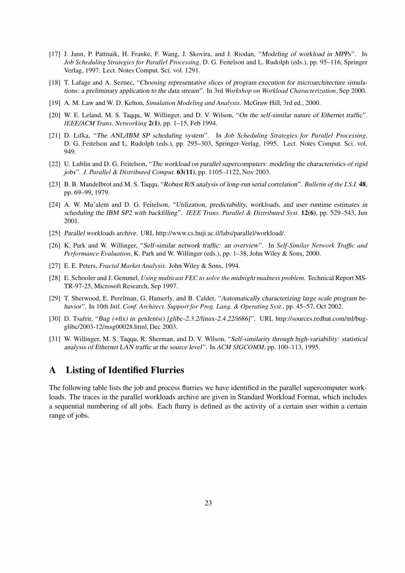
A Listing of Identified Flurries
The following table lists the job and process flurries we have identified in the parallel supercomputer work-loads. The traces in the parallel workloads archive are given in Standard Workload Format, which includesa sequential numbering of all jobs. Each flurry is defined as the activity of a certain user within a certainrange of jobs.
23
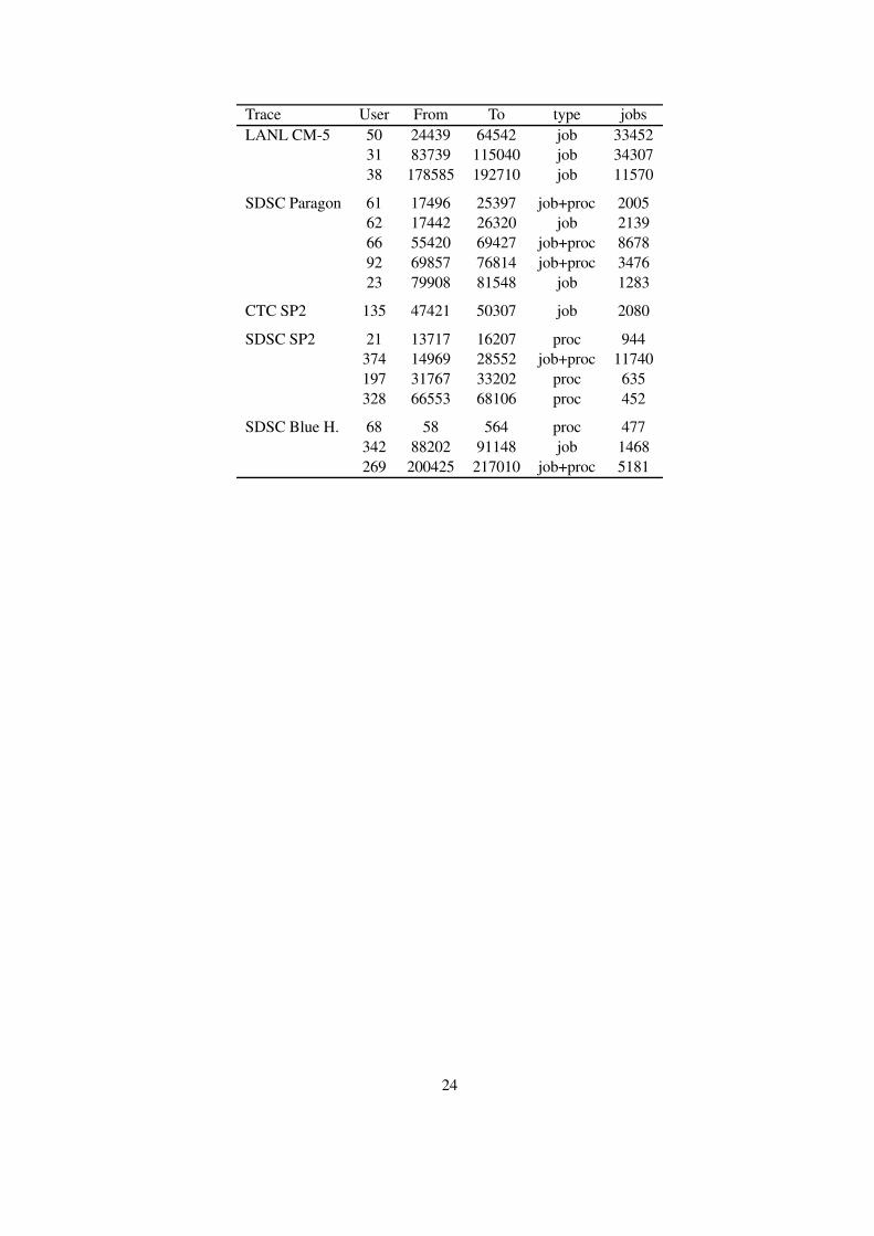
Trace User From To type jobsLANL CM-5 50 24439 64542 job 33452
31 83739 115040 job 3430738 178585 192710 job 11570
SDSC Paragon 61 17496 25397 job+proc 200562 17442 26320 job 213966 55420 69427 job+proc 867892 69857 76814 job+proc 347623 79908 81548 job 1283
CTC SP2 135 47421 50307 job 2080
SDSC SP2 21 13717 16207 proc 944374 14969 28552 job+proc 11740197 31767 33202 proc 635328 66553 68106 proc 452
SDSC Blue H. 68 58 564 proc 477342 88202 91148 job 1468269 200425 217010 job+proc 5181
24