data inter-comparisons of the cris interferometers on

Data Inter-comparisons of the CrISInterferometers on Suomi-NPP and NOAA-20Joe Kristl, Kori Moore, Mark Esplin, Ben Esplin, Deron Scott20 June 2018

1SDL/18-1113-

Outline

• Goals• Approach• Comparison Data Selection• Radiative Transfer Code Inputs• Initial Results• Next Steps

2SDL/18-1113-

Goal of this Effort• Monitor CrIS interferometers by direct data comparison

– Both sensor datasets must be consistent for maximum value– Continuous monitoring supports early problem detection

• SNPP and N-20 are in same orbit, 50 minutes apart– Simultaneous Nadir Overpasses (SNOs) never occur– Views overlap, but with geometry and time difference

• Current comparisons use SNO with intermediate reference(N20 – ref) – (SNPP – ref) = N20 – SNPP

– Spectral reference data sources are:• AIRS spectrometer (on Aqua satellite)• IASI interferometers A and B (on Metop satellites)

• This study investigates use of a radiative transfer code to create another reference for continuous comparisons

3SDL/18-1113-

CrIS Interferometer on NOAA-20/SNPP

4

Cross-track Infrared Spectrometer 2x Global Coverage Twice Daily

±50°Cross Track

Scans

EDR Algorithms

Decode Spacecraft

Data

SDR Algorithms

SNPP and NOAA-20 in Polar Orbit

3x3 array of CrIS FOVs (each at

14-km diameter)

Central or Regional Ground

StationsSDRs

RDRs

0.1

1

10

100

1000200 210 220 230 240 250 260 270 280 290

Temperature (K)

Pres

sure

(mb)

EDRs

SDL/18-1113-

Temporal and Spatial Separation

5

• View geometry: zenith (nadir) angles 10° to 60°– Azimuth angles: ~ 180° different

• Time separation: 50 minutes– Changing weather conditions– Solar effects (heating/cooling)

• Spatial resolution: Comparable to CrIS footprint (14 km nadir)

2018-02-18 OrbitsRed = SNPP 32702Grn = N-20 01305

Schematic viewing geometry

SDL/18-1113-

Clear Conditions Comparison Example

6

Spectral Radiance Brightness Temperature Difference

LWIR

MWIR

SWIR

SDL/18-1113-

ApproachN20(ν) – SNPP(ν) = ΔLatm(ν) + Lerror(ν)

ΔLatm(ν) = radiance difference due to ΔWX (atm, surface T)Lerror(ν) = error discrepancy of interest

• Use atmospheric radiative transfer code to calculate ΔLatm(ν)ΔLatm(ν) = RTcalc(ν)N20 - RTcalc(ν)SNPP

Then N20(ν) – SNPP(ν) - ΔLatm(ν) = Lerror(ν)• This study uses MODTRAN 6 as the radiative transfer code (RTcalc)

– 0.1 cm-1 band models, CorK, and line-by-line option– Convolved with sinc function to match CrIS resolution

• The real challenge lies in determining model inputs– Require atmospheric profiles that match each CrIS measurement to

compensate for weather condition differences

7SDL/18-1113-

Comparison Selection Criteria• Clear sky conditions

– Clouds are too variable over 50-minute time scale• For initial testing: clear sky ocean conditions• Forecast models include cloud cover outputs that support automatic

detection of clear areas– Combine results from all models for a robust result– Effective initial filter of CrIS data

• Currently use GIS software to create clear sky mask from weather model cloud cover, then extract CrIS view intersections within this clear area

• Plan to extend this to include clear sky land conditions– Eventual goal of automated selection for hands-off operation

8SDL/18-1113-

Radiative Transfer Model Inputs

• Difficult part is not the model, but rather the inputs to the model• Atmospheric inputs with sufficient fidelity to distinguish

differences on scales that matter to a CrIS comparison– Temporal: 50 minutes– Spatial: 20 km or less

• Regional models have needed temporal and spatial resolution– Global models are developing in same direction

• Primary data needed for CrIS bands– Altitude profiles of T, H2O, O3, CO2, CO, CH4, N2O– Surface temperature + emissivity

9SDL/18-1113-

Molecular Contributions to Spectrum

10

LWIR MWIR SWIRCrIS

Bands

SDL/18-1113-

Sources of Atmospheric Profile Data

• Global and regional numerical weather models used in this study

• Regional models meet resolution requirements but are incomplete– Daily forecast products (not archives) must be used– Missing ozone, end above the troposphere– Hybrid profiles necessary to fill in missing pieces

• The forecast models are steadily advancing in coverage/resolution• Anticipate global coverage with this resolution within a year or two

11

Temporal Spatial Model Update TimeStep Lat x Lon Footprint Coverage

GFS 6 hr 1 hr 0.25 28 km globalGEOS-FP 6 hr 1 hr, 3 hr 0.25 x 0.32 28 km global

RAP 1 hr 1 hr 0.11 11 km regionalHRRR 1 hr 1 hr 0.05 3 km regionalNAM 6 hr 1 hr 0.05 3 km regional

SDL/18-1113-

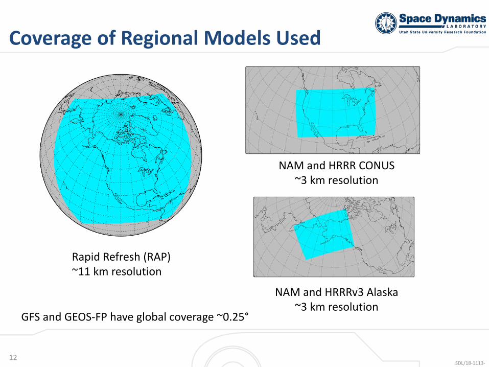
Coverage of Regional Models Used

12

Rapid Refresh (RAP)~11 km resolution

NAM and HRRRv3 Alaska~3 km resolution

NAM and HRRR CONUS~3 km resolution

GFS and GEOS-FP have global coverage ~0.25°

SDL/18-1113-

Additional Profile Data (not yet used)• Trace gas vertical profiles

– ECMWF – CAMS Near-Real-Time• O3, CH4, some NOx (but not N2O)

– NASA GEOS-FP• CO2 and CO

• Ocean surface temperatures• GFS high-resolution global skin temperature

– Hourly, ~11 km resolution• ECMWF 3 hr weather forecasts • ECMWF Hires• Re-analysis datasets (ERA-5)

13SDL/18-1113-

Creating MODTRAN Inputs• Profile data obtained through database queries of weather data

near spatial location of ground footprint and time• User-defined atmosphere profile inputs generated from this data

– Pressure, temperature, altitude, water, and ozone• When profiles are incomplete, the global models are searched and

provide data used to fill gaps and upper atmosphere• Surface temperature obtained from weather model • Additional inputs obtained from some models

– Visibility– Aerosol inputs

• Geometry created from satellite location and view angle

14SDL/18-1113-

Sample Atmospheric Profiles

• Composite profiles– Global models fill gaps and upper atmosphere

15

H2O

O3

SDL/18-1113-

Examples of Correction Improvement LWIR

16

• Green: Same residual N20 – SNPP• Red: Residual after SDL’s correction

• Green: Residual from N20 – SNPP• Black: MODTRAN correction (MSNPP – MN20)

SDL/18-1113-

MWIR Full-resolution Band

17



SDL/18-1113-

SWIR Full-resolution Band

18



SDL/18-1113-

Comparisons in Progress

• Initial Results– Reduce discrepancy from

~ 1 K down to the 0.1 K range

– Compensates for nadir angle differences well

– RAP and NAM model results performing better than HRRR

• Small sample size

19

RAP NAM HRRRLWIR AboveProf=3

BNum Ref New Chg New Chg New Chg0 0.775 0.097 0.678 0.079 0.695 0.157 0.6181 0.814 0.261 0.553 0.137 0.677 0.236 0.5782 1.660 0.071 1.588 0.184 1.475 0.082 1.5773 0.560 0.210 0.350 0.123 0.437 0.280 0.2804 0.567 0.233 0.334 0.136 0.431 0.292 0.2755 1.870 0.042 1.828 0.075 1.795 0.161 1.7086 2.063 0.029 2.034 0.100 1.963 0.065 1.999

1.187 0.135 0.119 0.182MWIR AboveProf=3


0.920 0.088 0.380 0.207SWIR AboveProf=3


1.141 0.180 0.197 0.201

SDL/18-1113-

Next Steps• Initial results show encouraging trends

– WX model data appears to have adequate temporal and spatial resolution to capture changes over the 50-minute interval between CrIS spectra

– Current sample too small for any statistical conclusions yet• MODTRAN 0.1 cm-1 band model option provides rapid answers

at required fidelity• SDL will work to refine these results and improve the profile

selection– Additional profile and surface data sources will be added– Additional test cases to be added for comparisons over more of

the sensor background signal range (near equator to poles)

20SDL/18-1113-

data inter-comparisons of the cris interferometers on

Documents