data fusion aided freeway analysis for highway capacity
TRANSCRIPT
Project ID: NTC2015-MU-R-05
Data Fusion Aided Freeway Analysis for Highway
Capacity Manual
(Final Report)
by
Behzad Aghdashi, Ph.D.
Research Associate, ITRE, NC State University
909 Capability Dr, Raleigh, NC
J. Lake Trask, Ph.D.
Transportation Analyst
Kittelson & Associates, Inc., Wilmington NC
for
National Transportation Center at Maryland (NTC@Maryland)
1124 Glenn Martin Hall
University of Maryland
College Park, MD 20742
March 2018


iii
ACKNOWLEDGEMENTS
This project received funding from the National Transportation Center @ Maryland
(NTC@Maryland), one of the five National Centers that were selected in this nationwide
competition, by the Office of the Assistant Secretary for Research and Technology (OST-R), U.S.
Department of Transportation (US DOT). Many thanks for the support provided by NTC. Our
thanks also go to Justin Babich who helped formatting and editing this report.
DISCLAIMER
The contents of this report reflect the views of the authors, who are solely responsible for the facts
and the accuracy of the material and information presented herein. This document is disseminated
under the sponsorship of the U.S. Department of Transportation University Transportation Centers
Program in the interest of information exchange. The U.S. Government assumes no liability for
the contents or use thereof. The contents do not necessarily reflect the official views of the U.S.
Government. This report does not constitute a standard, specification, or regulation.


v
TABLE OF CONTENTS
ACKNOWLEDGEMENTS ....................................................................................................... III
DISCLAIMER............................................................................................................................. III
TABLE OF CONTENTS ............................................................................................................ V
LIST OF TABLES .................................................................................................................... VII
LIST OF FIGURES ................................................................................................................. VIII
EXECUTIVE SUMMARY .......................................................................................................... 1
1.0 INTRODUCTION AND BACKGROUND .................................................................... 3
1.1 PROJECT OBJECTIVES: .................................................................................................. 3
1.2 LITERATURE REVIEW ................................................................................................... 4
1.2.1 Overview of Dynamic Traffic Assignment and the Cell Transmission Model .......... 4
1.2.2 Optimization Extensions to the Core CTM Formulation ............................................ 5
1.2.3 CTM Formulations and ATM Analysis ...................................................................... 6
1.2.4 Overview the Transportation Network Design Problems (TNDP) ............................. 6
1.2.5 HCM Calibration and Hourly Demand Profiles ......................................................... 7
1.2.6 Calibration of the CTM and Related Models .............................................................. 9
1.2.7 System Identification and Metaheuristics ................................................................... 9
2.0 FREEVAL AUTOMATIC SEGMENTATION ........................................................... 11
2.1 MAPS INTEGRATION.................................................................................................... 11
2.1.1 Google Maps JavaScript API .................................................................................... 11
2.1.2 Open Street Maps ...................................................................................................... 12
2.2 FREEVAL AUTOSEGMENTATION PROCEDURE .................................................... 12
2.2.1 Phase 1: Checking for Mainline Geometric and Capacity Changes ......................... 13
2.2.2 Phase 2: Identify Ramp Gore Points ......................................................................... 13
2.2.3 Phase 3: Marking Segment Influence Areas ............................................................. 13
2.2.4 Phase 4: Final Adjustments and Alternatives ........................................................... 13
2.3 DETAILED AUTOSEGMENTATION STEPS ............................................................... 13
2.4 IMPLEMENTATION INTO FREEVAL ......................................................................... 18
3.0 ESTIMATE DEMAND FOR FREEVAL ..................................................................... 21
3.1 PROPOSED FRAMEWORK ........................................................................................... 21
3.1.1 Profile-Based Encoding ............................................................................................ 22
3.1.2 Mixture Distribution Encoding ................................................................................. 23
3.2 COMPUTATIONAL STUDIES AND RESULTS ........................................................... 27
3.2.1 Simple Computational Example ............................................................................... 27
3.2.2 I-540 Case Study ....................................................................................................... 31
4.0 FREEVAL CALIBRATION .......................................................................................... 37
4.1 IMPORTANCE OF FREEVAL CALIBRATION ........................................................... 37
4.2 INTEGER PROGRAMMING APPROACH .................................................................... 37
4.2.1 Formulation of the MILP Model............................................................................... 38
4.2.2 Minimum and Maximum Relationships as Constraints ............................................ 39

vi
4.2.3 Issues Due to Computational Complexity ................................................................ 40
4.2.4 Small Computational Example and Results .............................................................. 40
4.3 A GENETIC ALGORITHM APPROACH ...................................................................... 42
4.3.1 Genetic Algorithm Overview .................................................................................... 42
4.3.2 Unifying Demand and Capacity Calibration............................................................. 44
4.3.3 Fitness Evaluation ..................................................................................................... 45
4.3.4 Genetic Encoding of the Capacity Calibration Parameters....................................... 46
4.3.5 Selection and Crossover ............................................................................................ 48
4.3.6 Mutation .................................................................................................................... 49
4.3.7 Computational Experiments and Numerical Results ................................................ 50
4.3.8 Phase 1 Calibration Results ...................................................................................... 52
4.3.9 Phase 2 Calibration Results ...................................................................................... 56
5.0 CONCLUSIONS ............................................................................................................. 62
6.0 REFERENCES ................................................................................................................ 64
vii
LIST OF TABLES
Table 1: Summary of the five parameters of each distribution ..................................................... 25
Table 2: Distribution parameter ranges......................................................................................... 25
Table 3: Parameters for each of the three random variables of the example mixture distribution 26
Table 4: Summary of the setup parameters for the GA runs ........................................................ 30
Table 5: Summary of the calibration results for the profile-based encoding runs ........................ 30
Table 6: Summary of the setup parameters for the profile-based GA runs .................................. 33
Table 7: Results summary of the GA Calibration Runs ............................................................... 33
Table 8: Breakdown of the mean absolute speed error of each segment in each time period for
three speed regimes using the profile-based encoding ......................................................... 34
Table 9: Summary of the setup parameters for the 3-distribution encoding GA runs .................. 35
Table 10: Summary of the distribution parameters for the 3-distribution encoding ..................... 35
Table 11: Results summary of the GA Calibration Runs ............................................................. 36
Table 12: Breakdown of the mean absolute speed error of each segment in each time period for
three speed regimes of the 3-distribution encoding calibration ............................................ 36
Table 13: Recommended ranges for the capacity calibration parameters .................................... 47
Table 14: Parameter minimum values and step sizes for the encoding example .......................... 48
Table 15: Summary of the average absolute speed errors for the uncalibrated facility ................ 50
Table 16: Facility travel times based on the target speeds compared to those from the un-
calibrated facility .................................................................................................................. 52
Table 17: Summary of the parameters used for the Phase 1 calibration ....................................... 53
Table 18: Summary results for the Phase 1 calibration run. All errors are the average absolute
difference in speed ................................................................................................................ 53
Table 19: Facility travel times based on the target speeds compared to those from the facility
after Phase 1 calibration ........................................................................................................ 55
Table 20: Summary of the parameters used for the Phase 2 calibration runs ............................... 56
Table 21: Summary results for the Phase 1 calibration run. All errors are the average absolute
difference in speed ................................................................................................................ 57
Table 22: Facility travel times based on the target speeds compared to those from facility after
Phase 2 calibration ................................................................................................................ 58
Table 23: Summary results for the Phase 1 calibration run, all errors are the average absolute
difference in speed ................................................................................................................ 60

viii
LIST OF FIGURES
Figure 1: Example fundamental flow-density diagram (Highway Capacity Manual 2016) ........... 5 Figure 2: Core freeway analysis calibration framework in the 6th edition of the HCM (Highway
Capacity Manual 2016) ........................................................................................................... 8 Figure 3: National default hourly demand profiles for weekdays and weekends on urban and
rural interstates ........................................................................................................................ 8 Figure 4: Example of integration of the Google Maps API to improve facility creation ............. 11 Figure 5: Facility with start and end points marked as segment boundaries ................................ 14
Figure 6: Example facility with geometric and capacity changes marked as segment boundaries
............................................................................................................................................... 14
Figure 7: Example facility with each ramp gore point marked as a candidate segment boundary14 Figure 8: In the case of an on-ramp followed by an off-ramp with an auxiliary lane, the candidate
boundaries should be shifted to account for influence areas, and the resulting segment is a
weave .................................................................................................................................... 15
Figure 9: Example facility with the first set of permanent segment boundaries from geometric
factors and ramp gore points ................................................................................................. 15 Figure 10: Example facility with candidate segment boundaries created due to ramp influence
areas ...................................................................................................................................... 15
Figure 11: Any influence area that passes a permanent segment boundary should be reduced to
match the existing boundary ................................................................................................. 16 Figure 12: When a small segment will be created between a candidate and permanent segment
boundary, the influence area should be increased to match the existing segment boundary 16 Figure 13: If influence areas between two adjacent ramps overlap, but the segment is not a weave
configuration, the candidate boundaries are made permanent, and an overlap (R) segment is
created ................................................................................................................................... 17 Figure 14: If influence areas of adjacent ramps do not overlap, but the candidate boundaries
create a small segment, the middle point between the two becomes a permanent segment
boundary ............................................................................................................................... 17
Figure 15: All remaining candidate segments should be valid and can be marked as permanent
segment boundaries ............................................................................................................... 17 Figure 16: Fully segmented example facility with each segment marked by type (B-Basic, N-On-
ramp, F-Off-ramp, W-Weave, R-Overlap) ........................................................................... 18 Figure 17: New FREEVAL interface allowing for visual placement of gore points along a facility
using Google Maps ............................................................................................................... 19
Figure 18: The interface allows an analyst to view satellite images to help determine additional
information about the facility................................................................................................ 20 Figure 19: Relationship between demand, observed flow rate, and bottleneck capacity ............. 21 Figure 20: Example of an input demand profile shape with a 15% search interval specified ...... 22 Figure 21: The skew normal distribution with varying values for the skewness parameter......... 24
Figure 22: The skew Cauchy distribution with varying values for the skewness parameter ........ 24 Figure 23: String to random probability density function conversion .......................................... 26
Figure 24: Probability density functions of the full mixture distribution and the component
random variables ................................................................................................................... 27

ix
Figure 25: Geometry of the example facility. The bottleneck resulting from the lane drop in
segment 26 creates two congestion regimes over the study period. ..................................... 28 Figure 26: Bimodal-AM Peak 25th Percentile demand profile used to allocate the AADT over the
study period ........................................................................................................................... 28 Figure 27: Left: Speed contour obtained after performing the HCM analysis that is used as the
target data set for calibration................................................................................................. 29 Figure 28: Comparison of the target speeds and the predicted speeds after calibration ............... 30 Figure 29: Comparison of profiles generated by the best and the worst of the GA calibration
runs, the “ground truth” profile is represented by the dotted line, while the predicted profile
is given by the solid line ....................................................................................................... 31
Figure 30: Geometry of the I-540 westbound case study facility ................................................. 31
Figure 31: Observed speed contour for the study period used as the target data set for the case
study example ....................................................................................................................... 32 Figure 32: Uncalibrated speed contour predicted after the initial demand allocation .................. 32 Figure 33: Predicted speed contour resulting from the calibration run with the lowest total speed
error ....................................................................................................................................... 33 Figure 34: Speed contour of the calibrated facility with the lowest total speed error .................. 36
Figure 35: Example of the mainline flow (MF) and the segment flow (SF) calculations with on-
ramps and off-ramps ............................................................................................................. 38
Figure 36: Geometry of the facility for the simple MILP computational example ...................... 41
Figure 37: Queue percentage for each segment of the facility for each time period .................... 41
Figure 38: Validation process for the predicted demands computed with the MILP model ........ 42 Figure 39: Effects of varying jam density values Kj,1 and Kj,2 on the volume density diagram
(Highway Capacity Manual 2016). ....................................................................................... 43 Figure 40: High-level process flow of the unified two-stage calibration process ........................ 45 Figure 41: Example of encoding three pre-breakdown CAFs and the facility-wide jam density
into binary strings based on the values of Table 14 .............................................................. 48 Figure 42: Demonstration of three common crossover operators ................................................. 49
Figure 43: HCM segmentation of 14.5-mile section of I-540 westbound near Raleigh, NC ....... 50 Figure 44: Speeds obtained from the real-world sensor data for Tuesday, August 19th, 2014 (top)
and those initially predicted by the FREEVAL computational engine for the un-calibrated I-
540 case study facility ........................................................................................................... 51 Figure 45: Comparison of the target speed contour (top) and the speed contour as predicted by
the partially calibrated facility after Phase 1 ......................................................................... 54 Figure 46: Comparison of target speed contour (top) and the speed contour as predicted by the
calibrated facility after Phase 2 ............................................................................................. 57 Figure 47: Chart showing the set of pre-breakdown CAFs for all segments of the facility as
estimated during the Phase 2 calibration process ................................................................. 59 Figure 48: Comparison of target speed contour (top) and the speed contour as predicted by the
methodology after the special case Phase 2 calibration with a single CAF .......................... 61


1
EXECUTIVE SUMMARY
The Highay Capacity Manual (HCM) is one of the widely used refercens in the transportation
engineerng. The 6th edition of HCM provides a multimodal framework to broaden the scope of
HCM applications. This project focused on the freeway facilities analysis which plays the core
role in other freeway analysis types in HCM. Other facility-based analysis in HCM is built on
freeway facilities methodology such as travel time reliability, Active Traffic and Demand
Management (ATDM), or Work Zone analyses.
FREEVAL is the offcial computational engine for HCM, performing freeway analysis. It is
freely avaible to download (freeval.org). It replicates the methods in the HCM, and offers the same
analysis types as offered by HCM such as travel time reliability analysis or etc. FREEVAL first
developed more than a decade ago using Excel/VBA. The 2015 version used Java as the platform
and as a result offered a lot of enhancements in terms of computational speed as well as GUI. This
project utilized FREEVAL computational engine and built its findings as additional packages for
FREEVAL.
This research focused on the use of avaible data sources to streamline the HCM freeway
analysis. Examples of availble data sources were investigated are a) online mapping tools and b)
sensor data providing speeds. These data sources can be utilized to aid analysts perform freeway
segmentation as well as demand estimation and calibration.
The research team investigated different online mapping services and evaluated information
that can be gathered through these data sources. Google Maps API selected to be the best data
provider for geometric data needs for freeway analysis. Beside this effort, the project team
developed a segmentation procedure that can divide a freeway strech into HCM segments. The
resulting HCM segments are completely matching with HCM definitions. The project team
implemented the developed segmentation procedure in FREEVAL. Google Maps API also
emplyed to assist analysts fill requried information (e.g. sections lengths) automatically. As a
result, the entire procedure of segmentatin automated in FREEVAL computational engine.
The project also developed methods to estimate demand and calibrate analysis based on
availble sensor data. The most uniform sensor database availble across US is probe-based speed
data. There are several number of probe-based speed data providers such as INRIX, Here.com,
and etc. The developed models to estimate demand and calibrate FREEVAL to target speed
profiles/contours tunes speed, capacity and demand adjustment factors. The proposed method
implemented in FREEVAL and can be invoked to perform demand estimation and analysis
calibration.


3
1.0 INTRODUCTION AND BACKGROUND
The Highway Capacity Manual (HCM) is a widely utilized reference document for various
planning and operational-level transportation analysis methods (Highway Capacity Manual 2016).
Among others, it provides a set of methodologies to evaluate freeway facility performance, as well
as freeway reliability analyses. Despite the macroscopic nature of the methods in the HCM, and
despite the availability of several software packages implementing the method, performing a
correct analysis is difficult and time consuming. This is largely due to 1) time-consuming
preliminarily data collection and preparation prior to the analysis, 2) difficulty in correct data
collection and data entry, and 3) lacking guidance on data needs for calibration and validation.
These factors are not comprehensively covered in the HCM, nor do procedures exist for
automating these processes. This research tried to address these shortcomings in order to assist
HCM users and agencies and ease the methodologies to be performed correctly.
Furthermore, the developed HCM-based calibration methodology can aid dynamic traffic
assignment and corridor-level capacity analysis, which is an increasingly useful tool for traffic
analysis and evaluation at the network level. How to understand the data needs and further calibrate
dynamic demand and supply elements for large-scale traffic regions and corridors is a challenging
issue from both theoretical and practical aspects. It is important and necessary to use observed
data, such as probe point-to-end travel time from probe-based data sources (e.g. INRIX) or sensor-
based flow and speed data, for constructing time-dependent simulation representations consistent
with real-world conditions.
The scope of this research effort is concentrated on "significant" non-recurring sources of
congestion, which are expected to have a high impact on the traveling public and are oftentimes
located on freeway facilities. As such, the FREEVAL tool is ideally suited for analysis, since it is
fundamentally based on the freeway facilities methodology in the 6th edition of HCM. The tool
has been effectively used in national level research to model the effects of recurring freeway
bottlenecks and was found to be significantly more efficient when compared to simulation-based
analysis tools. The reliability version of the FREEVAL considers non-recurring congestion
sources such as weather and incident’s impact which enables a comprehensive assessment of the
freeway facilities.
1.1 PROJECT OBJECTIVES:
The objectives of the proposed project were to:
1. Develop a data preparation framework and methodology for an HCM freeway facility
analysis, including the use of online mapping tools for facility segmentation;
2. Develop ‘demand estimation’ and ‘calibration’ methodologies to adjust demand and
capacity in conjunction with freeway characteristics such as capacity reduction due to
congestion.
3. Identify possible data sources that can be integrated into HCM (FREEVAL) analysis
framework for demand estimation, calibration and also validation;

4
The research approach built on existing HCM methodologies, the FREEVAL tool (the
computational engine for the HCM freeway facilities methodology), available online mapping
tools (Google map, open street map, etc.), as well as online data sources (e.g. INRIX, RITIS,
PEMS, etc). FREEVAL is the official computational engine for HCM freeway analysis. It has been
developed and updated at ITRE for more than a decade. The new version of FREEVAL is
developed in a Java environment and utilizes all capabilities of a multiplatform-programming
environment that assures the feasibility of possible connections to various online or offline data
sources, as well as performing more complex mathematical procedures such as optimizations.
However, the existing HCM procedure is limited to the core method and select extensions for
reliability analysis and others. It does not provide guidance on input data needs such as demand
input, calibration details, and integration with modern data sources. This research filled this gap,
and developed the necessary guidance for implementing agencies, assisted by automation of data
input and calibration procedures that streamline the application of the method.
1.2 LITERATURE REVIEW
1.2.1 Overview of Dynamic Traffic Assignment and the Cell Transmission
Model
An important analysis technique used in planning and evaluating freeway transportation
networks is Dynamic Traffic Assignment (DTA). DTA seeks to model “time-varying network and
demand interaction using a behaviorally sound approach" (Chiu et al., 2011). This research is
primarily interested in a subset of DTA consisting of equilibrium-seeking mesoscopic models, i.e.,
models whose resolution falls between microscopic and macroscopic models, but make use of
properties of both. DTA models are often used to evaluate travel times and costs of network
performance by modeling them as optimization problems. In these formulations, travel time and
cost become the objectives to be minimized and are subject to flow conservation and traffic
assignment constraints. Throughout the literature reviewed, two different traffic assignment
conditions were generally used for the DTA formulations. The first and simpler of the two
conditions is the System Optimum (SO) condition. Under SO assignment, the goal is to minimize
the travel time or cost of the system as a whole (Ziliaskopoulos, 2000). The second condition, User
Equilibrium (UE) or User Optimum (UO) assignment, differs from this in that each individual
driver seeks to minimize his/her travel time, even if it comes at the cost of total system performance
(Ukkusuri & Waller, 2008). This dynamic can be more difficult to capture in mathematical models,
but is generally thought of to be a more realistic representation. It should be noted that under free
flow conditions with little to no congestion, the two conditions will converge to the same answer,
but when congestion is high, the optimal solutions can differ greatly. An in depth survey on DTA
is given by Chiu et al. (2011). One of the more widely used DTA models is the Cell Transmission
Model (CTM), which was first proposed by Carlos Daganzo (1994). The CTM primarily consists
of a set of difference equations that simulate traffic flow on highways and use shockwaves to
model the backward (upstream) propagation of traffic congestion. The equations are presented as
a discrete approximation of the differential equations proposed by Lighthill, Witham, and Richards
(Lighthill & Whitham, 1955a,b; Richards, 1956). These original differential equations (often
referred to as the LWR equations) were developed by applying hydrodynamic flow theory to traffic
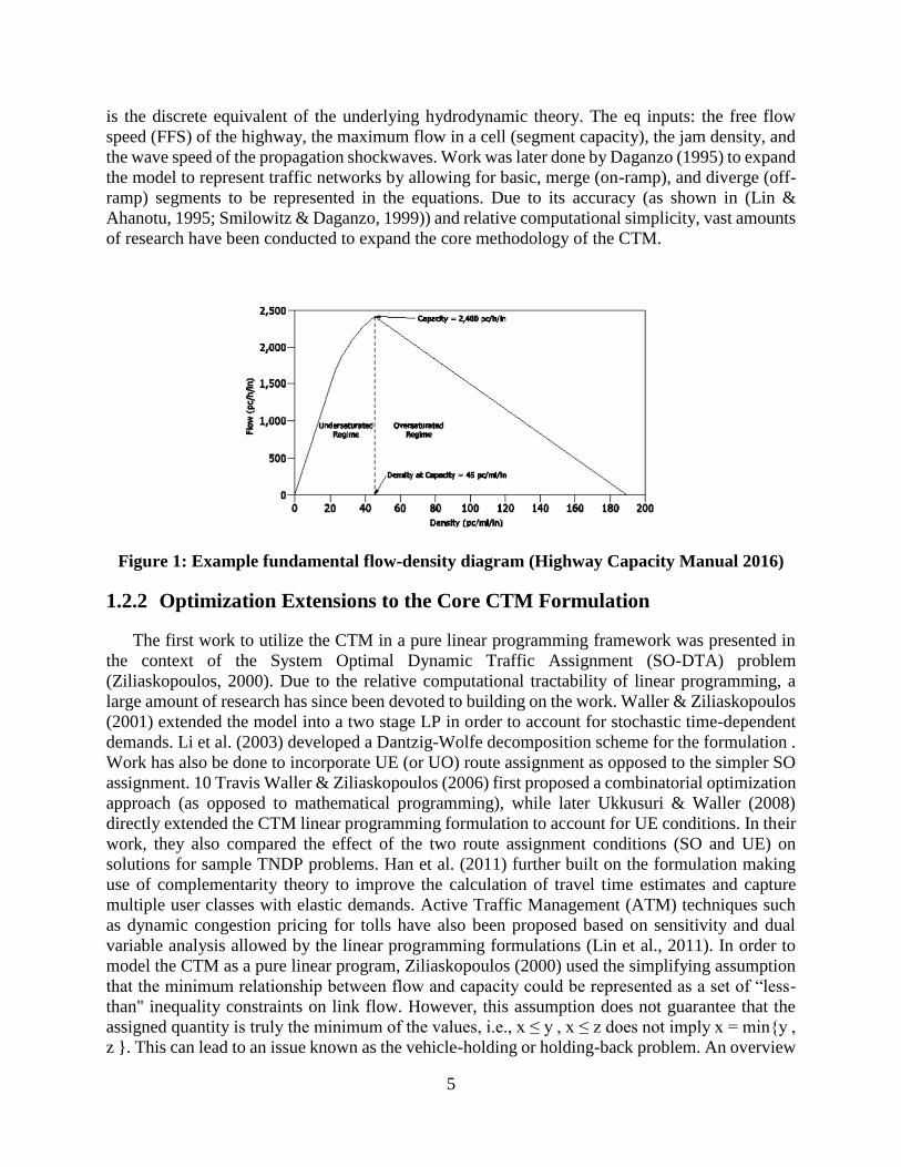
flow and analytically account for important concepts such as the Flow-Density diagram (Figure 1)
and the shockwave propagation of congestion. In his initial paper, Daganzo asserts that the CTM
5
is the discrete equivalent of the underlying hydrodynamic theory. The eq inputs: the free flow
speed (FFS) of the highway, the maximum flow in a cell (segment capacity), the jam density, and
the wave speed of the propagation shockwaves. Work was later done by Daganzo (1995) to expand
the model to represent traffic networks by allowing for basic, merge (on-ramp), and diverge (off-
ramp) segments to be represented in the equations. Due to its accuracy (as shown in (Lin &
Ahanotu, 1995; Smilowitz & Daganzo, 1999)) and relative computational simplicity, vast amounts
of research have been conducted to expand the core methodology of the CTM.
Figure 1: Example fundamental flow-density diagram (Highway Capacity Manual 2016)
1.2.2 Optimization Extensions to the Core CTM Formulation
The first work to utilize the CTM in a pure linear programming framework was presented in
the context of the System Optimal Dynamic Traffic Assignment (SO-DTA) problem
(Ziliaskopoulos, 2000). Due to the relative computational tractability of linear programming, a
large amount of research has since been devoted to building on the work. Waller & Ziliaskopoulos
(2001) extended the model into a two stage LP in order to account for stochastic time-dependent
demands. Li et al. (2003) developed a Dantzig-Wolfe decomposition scheme for the formulation .
Work has also be done to incorporate UE (or UO) route assignment as opposed to the simpler SO
assignment. 10 Travis Waller & Ziliaskopoulos (2006) first proposed a combinatorial optimization
approach (as opposed to mathematical programming), while later Ukkusuri & Waller (2008)
directly extended the CTM linear programming formulation to account for UE conditions. In their
work, they also compared the effect of the two route assignment conditions (SO and UE) on
solutions for sample TNDP problems. Han et al. (2011) further built on the formulation making
use of complementarity theory to improve the calculation of travel time estimates and capture
multiple user classes with elastic demands. Active Traffic Management (ATM) techniques such
as dynamic congestion pricing for tolls have also been proposed based on sensitivity and dual
variable analysis allowed by the linear programming formulations (Lin et al., 2011). In order to
model the CTM as a pure linear program, Ziliaskopoulos (2000) used the simplifying assumption
that the minimum relationship between flow and capacity could be represented as a set of “less-
than" inequality constraints on link flow. However, this assumption does not guarantee that the
assigned quantity is truly the minimum of the values, i.e., x ≤ y , x ≤ z does not imply x = min{y ,
z }. This can lead to an issue known as the vehicle-holding or holding-back problem. An overview
6
of the holding-back problem as well as a survey of the work done to account for it was compiled
by Doan & Ukkusuri (2012). Lo (2001) proposed accounting for this nonlinearity by incorporating
integer linear constraints that effectively turn sets of constraints on or off, though the work was
mostly investigated for its use in signal control applications. In a similar vein, Tampère & Immers
(2007) proposed the use of the Heaviside function for the approach. Zheng & Chiu (2011)
addressed the issue by proving that the single destination system optimal dynamic traffic
assignment (SD SO-DTA) problem is equivalent to the earliest arrival flow (EAF) network
problem, and developed a network flow algorithm that eliminated vehicle holding in basic and
merge segments (but not necessarily for diverge segments). Doan & Ukkusuri (2012) presented
multiple formulations to completely remove vehicle-holding under SO routing for problems with
multiple destinations. The removal of vehicle-holding was achieved by using complementarity
constraints and converting them to a nonlinear programming model, as well as by incorporating
mixed integer programming (MIP) techniques. Next, Ukkusuri et al. (2012) extended the
techniques to handle the UE conditions. Unfortunately, each of these formulations requires
assumptions that may not accurately reflect realistic conditions, and in addition still contain some
nonlinearities or non-convexities (Zhu & Ukkusuri, 2013). Further, in all of the previously
mentioned papers the authors acknowledge that the formulations are still impractical for larger and
more realistic sizes of networks. Another linear complementarity approach was developed by
Zhong et al. (2013) in order to better deal with the nonlineararity of the state jump conditions and
hard nonlinear min functions. The proposed formulation readily extends to both DTA and TNDP
analysis, and while not as com11 putationally efficient as pure LP formulations, it benefits from
the existing work done on linear complementarity problems (LCP) (Hu et al., 2012). More
recently, Zhu & Ukkusuri (2013) were able to develop a pure linear programming solution to the
vehicle-holding problem for the SD SO-DTA problem by introducing an easily computable
penalty function into the formulation. Sun et al. (2014) extended this to incorporate demand
uncertainty and developed an adjustable robust optimization (ARO) linear programming
formulation.
1.2.3 CTM Formulations and ATM Analysis
The CTM formulation and its extensions have also been used to tune ATM strategies. Gomes
& Horowitz (2006) developed the Asymmetric Cell Transmission Model (ACTM) to compute
optimal ramp metering rates. While the ACTM formulation remains nonlinear, the authors proved
sufficient conditions under which the globally optimal solution could be found through the use of
a single linear program. Unfortunately, these sufficiency conditions were rather constrictive, and
often highly unrealistic of true freeway conditions. Finding a lack of in-depth theoretical results
concerning the CTM/MCTM, Gomes et al. (2008) further investigated the properties of congested
and uncongested equilibria for the model and interpreted the findings with respect to the
effectiveness of ramp metering strategies. The authors found that optimally computed ramp
metering strategies can reduce congestion and travel time on freeways, and that the strategies do
more than just move the congestion to on-ramps. A dynamic on-line method to determine Variable
Speed Limits (VSL) has been proposed by Li et al. (2014), with benefits stemming from the low
computational cost of the CTM vs the more complex existing VSL algorithms.
1.2.4 Overview the Transportation Network Design Problems (TNDP)
Beyond supporting sensitivity analysis, optimization frameworks can also provide a direct path
to finding ways of improving existing transportation networks. Most problems of this nature fall

7
under the umbrella of Transportation Network Design Problems (TNDP). These problems seek to
provide an optimization model for the selection of network improvements. For example, if funds
for road widening are available, a TNDP formulation could be used to select the optimal portion
to be widened. There are a number of appropriate ways to formulate a problem such as this, but
often the model would seek to maximize the post-improvement traffic flow, while simultaneously
minimizing construction costs, all while satisfying the system’s flow conservation and traffic
assignment constraints. DTA and TNDP have many important applications beyond just their initial
scope. They can be used to improve reliability analysis of transportation networks, especially under
abnormal conditions such as evacuations (Lim et al., 2015; Malveo, 2013; Yao et al., 12 2009).
Due to the interplay between the equilibrium constraints and the multiple objective functions,
single level TNDP formulations are generally nonconvex and nonlinear. These types of problems
are known to be at least NP hard (Zeng & Mouskos, 1997). To regain some linearity, TNDP is
often formulated as a bilevel program, i.e., one with an upper level and a lower level objective
function. Despite the inherent difficulty in finding a solution for formulations such as these, it is
still important that at least a near globally optimum solution be found. As such, heuristic algorithms
have often been found to be the best choice to efficiently seek an optimal or near-optimal solution.
In recent years, much research has been conducted into the use of metaheuristic techniques such
as genetic algorithms (GA), simulated annealing (SA), and tabu search for extending and solving
TNDP formulations (Delbem et al., 2012; Juan et al., 2012; Karoonsoontawong & Waller, 2006;
Luathep et al., 2011; Mudchanatongsuk et al., 2008; Xu et al., 2009; Zeng & Mouskos, 1997).
1.2.5 HCM Calibration and Hourly Demand Profiles
The 6th edition of the Highway Capacity Manual (2016) provides guidance on how to address
model calibration in the form of a five-step process as shown in Figure 2. The first step requires
the user to 36 gather the required input data for the model including geometric aspects, segment
free flow speeds (FFS), and initial demand volume estimates for the mainline and ramps at each
analysis period of the study period. No guidance is provided to address the process of initial
demand estimation. The manual breaks the calibration adjustment process into three pieces: free
flow speed calibration, bottleneck capacity calibration, and demand adjustment. Free flow speeds
can be calibrated using observed measures for uncongested or off-peak periods. For bottleneck
capacity calibration, the HCM advises a trial and error strategy. In the event the location and or
severity of congestion predicted by the model does not match that of an observed set of target
performance measures, the manual recommends that an analyst repeatedly adjust the capacity of
bottleneck segments by 50 pc/h/ln until an acceptable level of matching is achieved. Identification
of bottleneck segments is left up to the analyst’s knowledge of the facility. For demand estimation,
the manual advises that an analyst manually adjust volumes in increments of 50 pc/h/ln until
predicted model travel times and bottleneck queue lengths are within a specified margin of error.

8
Figure 2: Core freeway analysis calibration framework in the 6th edition of the HCM
(Highway Capacity Manual 2016)
In order to estimate the initial set of demand inputs, an analyst generally makes use of an
average annual daily traffic (AADT) value projected into individual demand volumes using an
hourly demand profile. An hourly demand profile provides a breakdown of the percentage of an
AADT value occuring during each hour of the day. Individual profiles are often highly specific to
the each 37 location, but general trends are common across most facilities. Demand profiles for
weekdays are often bimodal in that they contain two clear peaks. In this case, one peak typically
corresponds to travelers on their morning commute, and one corresponds to travelers commuting
home from work in the evenings. In contrast, weekend profiles are often unimodal, or have a single
peak, that builds more slowly throughout the day. Hallenbeck et al. (1997) developed a set of
national default profiles for weekdays and weekends, broken down into both urban and rural
categories. Both bimodal and unimodal behavior are reflected in the national default profiles,
shown in Figure 3.
Figure 3: National default hourly demand profiles for weekdays and weekends on urban
and rural interstates

9
Additionally, a study conducted for the state of North Carolina provides a further level of detail
and divides the profiles into 3 default categories: unimodal, bimodal with an AM peak, and
bimodal with a PM peak (NCDOT, 2016). Figure 2, above, shows examples of each of these three
types. The unimodal profiles are very similar to the weekend category of profiles, while the
bimodal profiles provide two variations of the weekday profile. Further, six additional profile
shapes are provided for each of three main profile types. These represent the minimum, the 25th
percentile, the average, the 75th percentile, the maximum, and median of all profiles generated
from the collected data.
1.2.6 Calibration of the CTM and Related Models
The cell transmission model is commonly used as a basis for automated density estimation and
calibration approaches. Some of the earliest work on this is presented by Munoz et al. (2003) who
develop the modified cell transmission model (MCTM) and the switching mode model (SMM).
This formulation differs from Daganzo’s basic CTM in three key ways. First, cell densities are
used as state variables as opposed to cell occupancy, directly leading to the second difference in
that the 38 MCTM can handle non-uniform cell lengths. Lastly, the formulation allows congested
conditions at the downstream end of a facility. These changes lead to some nonlinearities in the
difference equations regarding moving congestion wavefronts, so the authors develop the SMM to
return to a piecewise linear formulation. The SMM accounts for five different congestion status
modes that allow the model to switch between several sets of linear difference equations. The
authors are also able to show that the CTM and the MCTM/SMM can estimate demand within
freeway facilities with reasonable accuracy. A fair amount of density estimation research has come
out of the development of the MCTM and the SMM. Muñoz et al. (2004) propose a methodological
calibration procedure for the CTM/MCTM and further show the methods accurately estimate
density on longer stretches of freeway. This procedure is further explored by Zhong et al. (2014),
but their proposed nonlinear optimization framework again has the deficiency of an inability to
reliably find globally optimal solutions. The MCTM/SMM has been extended to included
stochastic variations in traffic, especially with respect to their effects on the fundamental flow-
density diagram. The Stochastic Cell Transmission Model (SCTM) directly incorporates stochastic
noise into the parameters of the fundamental diagram (Sumalee et al., 2011). Pascale et al. (2013,
2014) develop an alternative approach in which they use a Bayesian framework to account for
stochasticity, and propose a particle filtering approach to estimate density. Both methods are
shown to be reliably accurate in matching sample detector data. Most recently, a robust switching
approach for the SMM is introduced by Morbidi et al. (2014) in situations where the congestion
wave speed is unknown. Similar alternatives to the mechanisms of the MCTM/SMM for state
detection have also been developed. Stankova & De Schutter (2010) use a jump Markov linear
model (JMLM) to account for switching between free-flow and congested states, while Aligawesa
and Hwang propose a State Dependent Transition Hybrid Estimation (SDTHE) algorithm
motivated by the SMM but with improved state detection. Further research has been conducted
into density estimation and state prediction loosely based on the LWR equations and the CTM,
though most of the methods developed rely on relaxations and heuristics to even attempt to find
solutions (e.g., Lu et al. (2013) and Ma et al. (2015)).
1.2.7 System Identification and Metaheuristics
System identification was initially developed as a technique to construct mathematical models
of dynamic systems based on observed data (Ljung, 2010). The approach provides an effective

10
way of modeling systems where relationships between inputs and outputs are either unknown or
poorly understood to the point where an exact model cannot be built. For the approach, systems
are 39 generally classified in terms of a "transparency" on the scale between white and black. A
“white-box" model of a system is one where all relationships are known and have been defined.
For a “black-box" model little to nothing of the true relationships are known or can be defined (De
Nicolao, 1997). There also exist a number of variations of “grey-box" models that fall between the
two extremes where varying amounts of information are known (Ljung, 2010). In approaching a
grey-box model, a basic understanding of the relationships is assumed, but the complexities are
not fully or explicitly considered. Metaheuristics are a class of search approaches that “permit an
abstract level of description" and are used to “effeciently explore the search space in order to find
(near-) optimal solutions" (Blum & Roli, 2003). At their core, metaheuristics are not problem-
specific, but implementations can make use of “domain-specific knowledge...controlled by the
upper level strategy" (Blum & Roli, 2003). This lack of specificity paired with an abundance of
flexibility makes metaheuristic approaches particularly useful for solving grey or even black-box
system identification problems. There are a wide variety of types of metaheuristics that have been
developed including but not limited to simple local search techniques, evolutionary algorithms,
simulated annealing, and artificial neural networks (Gendreau & Potvin, 2005). A genetic
algorithm (GA) is an evolutionary search metaheuristic commonly used for complex optimization
problems where the underlying mathematics preclude the use of classical approaches. The
approach draws from the processes of evolution and natural selection in order to generate an
optimal or near-optimal solution by “evolving” a pool of candidate solutions over time (Goldberg,
1989). Each candidate solution is represented as an individual organism, with the decision
variables of the problem encoded as the organism’s “genes". An evaluation function is defined in
order to calculate the fitness of a candidate solution based on these genes. By choosing an encoding
and fitness function such that the problem is framed as a minimization or maximization of fitness,
fitnessbased “competition" can be used to make statements on the quality of one candidate solution
versus another. In this way, the fitness function is essentially analogous to the objective function
of classical optimization techniques like linear programming. The most critical aspect of using a
GA is the process of defining the encoding of a candidate solution as the genes of an organism. In
fact, the key underlying assumption to the GA approach is that high-quality solutions will contain
common “building blocks" in their encoded genetic material (Mitchell, 1998). Maintaining these
blocks within a population of organisms, and combining them with other “good" blocks should
then theoretically lead to the discovery of better solutions. Blocks can be combined through the
use of a crossover operator that represents the “mating" of organisms. While real-valued encodings
are occasionally used, most encodings consist of some type of binary representation of the solution.
This allows for a straightforward realization of genetic building blocks 40 (e.g., small binary
patterns such as “010" or “110"), as well as providing a simple notion of crossover through
exchanging binary digits.

11
2.0 FREEVAL AUTOMATIC SEGMENTATION
This section discusses the research team’s efforts to implement automatic segmentation
procedure for FREEVAL/HCM. In order to achieve automatic segmentation being useful and
applicable for users, first a mapping serice should be added to FREEVAL to assist users to define
the spatial scope of the analysis. The first part of this section discusses availble online mapping
services that can be incorporated in FREEVAL. The second part introduces a systematic procedure
to break freeway strech into HCM segments.
2.1 MAPS INTEGRATION
2.1.1 Google Maps JavaScript API
Google Maps has various free APIs available. The Directions, Distance Matrix, Geocoding,
and Roads APIs can use HTTP requests to query the desired data. In FREEVAL A JFX web panel
is created in Java Swing so that the Google Maps JavaScript API can be used. The API Reference
can be found here: https://developers.google.com/maps/documentation/javascript/3.exp/reference.
The JavaScript API incorporates the other APIs as services. For example, a connection with
the Directions API can be made to pass end points and receive a path of points in between. The
drawing service can use that path to draw a route. In the case of the JavaScript API, an API key is
only required to track access to a project. Without a key, the API limitations are more relaxed since
it is counted by session rather than by project. Google Maps has a significant set of features
available all in one place and it is highly documented and supported online.
Figure 4: Example of integration of the Google Maps API to improve facility creation

12
The Google Maps Roads API was initially investigated because of its ability to simply snap
points to a road and interpolate a path as the user clicks on the map. However, this came with a
severe sever limitation for allowable distance between points. A more elegant solution was found
using the Google Maps Directions API. The Directions API allows the user to place multiple points
on the map and receive a calculated route between them regardless of the distance.
2.1.2 Open Street Maps
Open Street Maps stores data inside of “Ways” which are segments of “Nodes” which are
coordinates. Metadata stored in Ways include things such as the speed limit and number of lanes,
however this information is not always present and can be very sparse depending on the area.
There is some ambiguity here as well. A segment on a road with two oncoming lanes, a middle
lane, and two ongoing lanes will have 5 lanes. A road segment with two lanes on each side of a
divider like Western Boulevard will return 2 lanes. A segment that ends at an intersection may
have a left turn lane, a right turn lane, and the oncoming traffic lane, so this segment returns 3
lanes. This data is reported by users so they may not follow a standard practice.
The Open Street Maps API is for editing the maps only. Reading Open Street Map data can be
done with the Overpass API. The Overpass API is a third party service and has a couple of public
instances: http://wiki.openstreetmap.org/wiki/Overpass_API. The Overpass API acts as a database
over the web so that data can be queried from Open Street Maps. Overpass API queries can be
tested on the web by running them with Overpass Turbo here: http://overpass-turbo.eu. Other third
party tools must be used to find routing information using Open Street Map data. These tools
usually have limited API requests allowed for free before pricing plans are required.
2.2 FREEVAL AUTOSEGMENTATION PROCEDURE
The first step in creating a model for analysis with the HCM’s freeway facilities methodology
is to determine the length of freeway being modeled, and divide into “segments” using the
manual’s specified guidance. The HCM accounts for five separate types of segments: basic, merge,
diverge, weaving, and overlap. A merge segment represents an on-ramp and its resulting influence
area, while a diverge segment is an analogous representation of an off-ramp. A weave segment
represents an on-ramp followed by an off-ramp that includes one or more auxiliary lanes
connecting the two ramps. An overlap segment exists when the influence areas of adjacent on and
off-ramps overlap and no auxiliary lane exists. Lastly, a basic segment is any other non-ramp
stretch of freeway.
While it is straightforward to identify major geometric changes and ramps for a facility, the
determination of the corresponding HCM compatible segments can be both challenging and time-
consuming. Further, HCM segmentation is highly unlikely to correspond to existing TMC
segments over which data is collected by a number of organizations. As such, manual
segmentation of a facility represents a major challenge to using the HCM methodology. This work
develops a new “autosegmentation” procedure based on the segmentation rules of the HCM in
order to reduce the burden placed on an analyst and greatly simplify the facility creation process.
The autosegmentation procedure consists of four main phases, as described in the subsequent
sections. Following that, the procedure is further broken down into 12 individual steps, and each

13
is presented with a detailed description. An example facility is segmented using the 12 steps and
presented alongside the description of each step.
2.2.1 Phase 1: Checking for Mainline Geometric and Capacity Changes
The first step identifies all geometric and capacity related changes that occur on the mainline
of the facility. These include land drops and lane additions, as well as changes in the speed limit.
These represent permanent segment breaks that are not affected by any potential adjustments
occurring in subsequent steps.
2.2.2 Phase 2: Identify Ramp Gore Points
In this step, all “gore points” of the facility are identified by the analyst. A gore point is found
at each ramp (both on and off-ramps) of the facility. Gore points do not represent segment
boundaries, but rather will be used to determine segment type (merge, diverge, weaving) and will
adjusted upstream or downstream in the following step to account for influence areas.
Weaving segments are also identified at this step. If the procedure finds that an on-ramp gore
point is followed by an off-ramp gore point, and that an auxiliary lane exists between the two
points, then the two gore points represent the ends of a weaving segment. However, these gore
points do not represent the segment boundary, as they must be adjusted to account for the weave
influence areas.
2.2.3 Phase 3: Marking Segment Influence Areas
The HCM segmentation procedure requires that (when possible) both on-ramp and off-ramp
segments include 1500ft influence areas. Hence, for each gore point from the previous step
denoting an on-ramp, the resulting merge segment’s downstream boundary is created 1500ft
downstream of the gore point. Analogously, for each gore point denoting an off-ramp, the resulting
diverge segment’s upstream boundary is created 1500ft upstream of the gore point. For each
weaving segment, the gore points marking the on-ramp and off-ramp are shifted upstream and
downstream, respectively, by 500ft.
2.2.4 Phase 4: Final Adjustments and Alternatives
In many cases, it is possible that the segment boundaries created in the previous steps will
create segmentations that include configurations that are either invalid entirely or conflict with
some of the HCM’s recommendations (i.e. segments shorter than the minimum length threshold).
To account for these occurrences, some of the segment boundaries can be shifted (especially those
related to influence areas) in order to eliminate these issues.
Any issues that arise create alternative potential segmentations from which to choose. The
analyst will be responsible for deciding which issues to address and how to address them, and
should make the decision based on their knowledge of the facility being modeled.
2.3 DETAILED AUTOSEGMENTATION STEPS
Step 1: The start and end points of a facility are permanent segment boundaries

14
Figure 5: Facility with start and end points marked as segment boundaries
Step 2: All changes in number of lanes and speed limit/free flow speed are permanent segment
boundaries. (Note: Accel/deccel lanes do not count as lane changes).
Figure 6: Example facility with geometric and capacity changes marked as segment
boundaries
Step 3: Identify all ramp gore points and mark as potential segment boundaries.
Figure 7: Example facility with each ramp gore point marked as a candidate segment
boundary
Step 4: Check to see if an auxiliary lane exists between all sets of adjacent on-ramp and off-ramp
gore points. If an auxiliary lane exists, then the two gore points form a weave segment. Next,
shift the on-ramp gore point 500ft upstream, and shift the off-ramp gore point 500ft downstream
to account for weave influence areas, and mark the shifted gore points as permanent nodes and
the result segment as a weave. (Note: if a permanent or candidate segment boundary is within the
500ft influence for the upstream or downstream end, the gore point shift is stopped at the
segment boundary.)

15
Figure 8: In the case of an on-ramp followed by an off-ramp with an auxiliary lane, the
candidate boundaries should be shifted to account for influence areas, and the resulting
segment is a weave
Step 5: Mark all remaining gore point candidate boundaries as permanent segment boundaries.
Figure 9: Example facility with the first set of permanent segment boundaries from
geometric factors and ramp gore points
Step 6: Determine 1500ft from and to on-ramp and off-ramp gore points, respectively, and mark
them as potential segment boundaries.
Figure 10: Example facility with candidate segment boundaries created due to ramp
influence areas
Step 7: For each new potential boundary, check to see if the 1500ft influence area has passed a
segment boundary. If it has, then reduce the 1500ft distance to be aligned with the segment
boundary.

16
Figure 11: Any influence area that passes a permanent segment boundary should be
reduced to match the existing boundary
Step 8: For each new potential boundary, check to see if the 1500ft influence area creates a short
(less than the minimum segment length threshold) segment with an adjacent permanent segment
boundary. If this occurs, increase the 1500ft threshold to match the adjacent segment boundary.
Figure 12: When a small segment will be created between a candidate and permanent
segment boundary, the influence area should be increased to match the existing segment
boundary
Step 9: For each new potential boundary, check to see if the 1500ft influence areas extending
from each pair of adjacent on and off-ramp segment boundaries (with NO auxiliary lane)
overlap. If the overlap area is larger than the minimum segment length threshold, mark the
candidates as segment boundaries, with the newly created segment being an overlap (R) segment
(the resulting layout will be ONR-R-OFR). If the overlap area is smaller than the threshold,
select the middle point between the two candidate boundaries as the permanent segment
boundary.

17
Figure 13: If influence areas between two adjacent ramps overlap, but the segment is not a
weave configuration, the candidate boundaries are made permanent, and an overlap (R)
segment is created
Step 10: Check to see if any pair of adjacent candidate segment boundaries will create a segment
shorter than the minimum length threshold. If an instance is found, merge the two candidates
into a single permanent segment boundary placed at the middle point between the two former
candidate locations.
Figure 14: If influence areas of adjacent ramps do not overlap, but the candidate
boundaries create a small segment, the middle point between the two becomes a permanent
segment boundary
Step 11: Mark any remaining candidate segment boundaries as permanent segment boundaries.
Figure 15: All remaining candidate segments should be valid and can be marked as
permanent segment boundaries

18
Step 12: Mark any segment that has not already been marked as merge, diverge, weave or
overlap as a basic segment.
Figure 16: Fully segmented example facility with each segment marked by type (B-Basic,
N-On-ramp, F-Off-ramp, W-Weave, R-Overlap)
2.4 IMPLEMENTATION INTO FREEVAL
The autosegmentation procedure as described in the previous sections has been implemented
into the FREEVAL computational engine for this project. The procedure is integrated into the
program with a new interface utilizing the Google Maps Javascript API. The interface displays a
set of Google Maps tiles in order to allow analysts to visually mark gore points for the facility
being modeled. This provides a much easier method for creating a facility.
An analyst begins by first placing a marker at the start of the facility. Next, the analyst proceeds
to mark all gore points for geometric changes, on-ramps, and off-ramps. Lastly, the analyst places
a marker indicating the end of the facility.
As markers are placed on the map, a table is created at the top of the interface. The table
includes alternating columns for “nodes” and “sections,” which correspond to gore points and the
links between them, respectively. The Google Maps API allows for the route along the freeway
between each pair of adjacent gore points to be automatically calculated and drawn, and the length
of the routed path of each section is given in the table. The interface allows each routed section of
the facility to be split into two, creating an additional gore point, or any two adjacent sections can
be merged by removing the gore point connecting them. Any gore point placed on the map can be
repositioned if necessary by simply dragging and dropping the map marker.

19
Figure 17: New FREEVAL interface allowing for visual placement of gore points along a
facility using Google Maps
The table also allows the analyst to fill in key geometric and capacity parameters required by
the segmentation procedure. The principal required value is the number of mainline lanes for each
section (from which the procedure identifies auxiliary lanes and weave segments), but an analyst
can also enter values for the speed limit, the number of ramp lanes, the exit number, and a name
label for each node. These parameters will be carried through the segmentation process and
automatically populated into the facility inputs once the segmentation procedure is complete.
Analysts can determine these values in a number different of ways. Previously, the values
could only be determined using an analyst’s existing knowledge of the facility, or by consulting
additional outside maps and data sources. This can still be done, but many of the values can now
be determined directly in the interface by way of switching to the satellite view of the facility. For
example, by visually inspecting the satellite images, an analyst can determine the number of
mainline lanes for each section. The satellite images can also be used to determine the location of
certain geometric changes, such as lane drops and lane additions.

20
Figure 18: The interface allows an analyst to view satellite images to help determine
additional information about the facility
Once all gore points have been marked and the analyst has provided the key input parameters,
the autosegmentation described previously is run. At the completion of the procedure, an
automated check is run to determine if any issues arose during the segmentation process (e.g.
unavoidable short segments). If no issues are found, the analyst is presented with a set of global
input parameters that can be adjusted if desired, and the HCM seed file is created.
If the automated check does find one or more segmentation issues, the analyst is presented
with a set of options that allow each issue to be addressed individually, or ignored if it is truly
unavoidable. It is also possible that issues or improper segmentations can arise due to gore points
being placed incorrectly, or incorrect determination of the required inputs (e.g. number of mainline
lanes). Consequently, the analyst is also allowed to return to the map and make adjustments as
necessary.

21
3.0 ESTIMATE DEMAND FOR FREEVAL
The freeway facilities methodology of the HCM is tightly built on demand volumes as the
main inputs for all freeway segments. These demand volumes are converted into densities and
used to estimate flow and congestion. While demand volumes are the critical input for the freeway
facilities analysis, they are mostly unknown in real-world situations and hence must be estimated
from data provided by a variety of types of sensors (i.e. loop detectors or manual counts).
Unfortunately, these sensors can only indicate the actual flow rates, travel times, speeds, observed
densities and other measures that are generally considered outputs of the methodology. These types
of readings often differ from actual demand volumes, especially at times when a queue is present
on the facility, as shown in Figure 19. This puts a challenge on the agencies using the methodology
to accurately estimate demand volumes that can produce the desired flow rates in the analysis.
Figure 19: Relationship between demand, observed flow rate, and bottleneck capacity
3.1 PROPOSED FRAMEWORK
A genetic algorithm metaheuristic framework is developed to address the challenges of
demand estimation in the context of model calibration. Two encoding approaches for the problem
are proposed based on the quality of available data. One approach makes use of existing
knowledge of hourly demand profiles, while the second utilizes mixture distributions of random
variables in order to allocate demand over the course of a study period when the behavior is
unknown. A genetic algorithm is then used to manipulate the individual demand inputs to find a
set of overall volumes that minimizes the errors between predicted outputs and a set of target real-
world performance measures (e.g., segment speeds).
22
3.1.1 Profile-Based Encoding
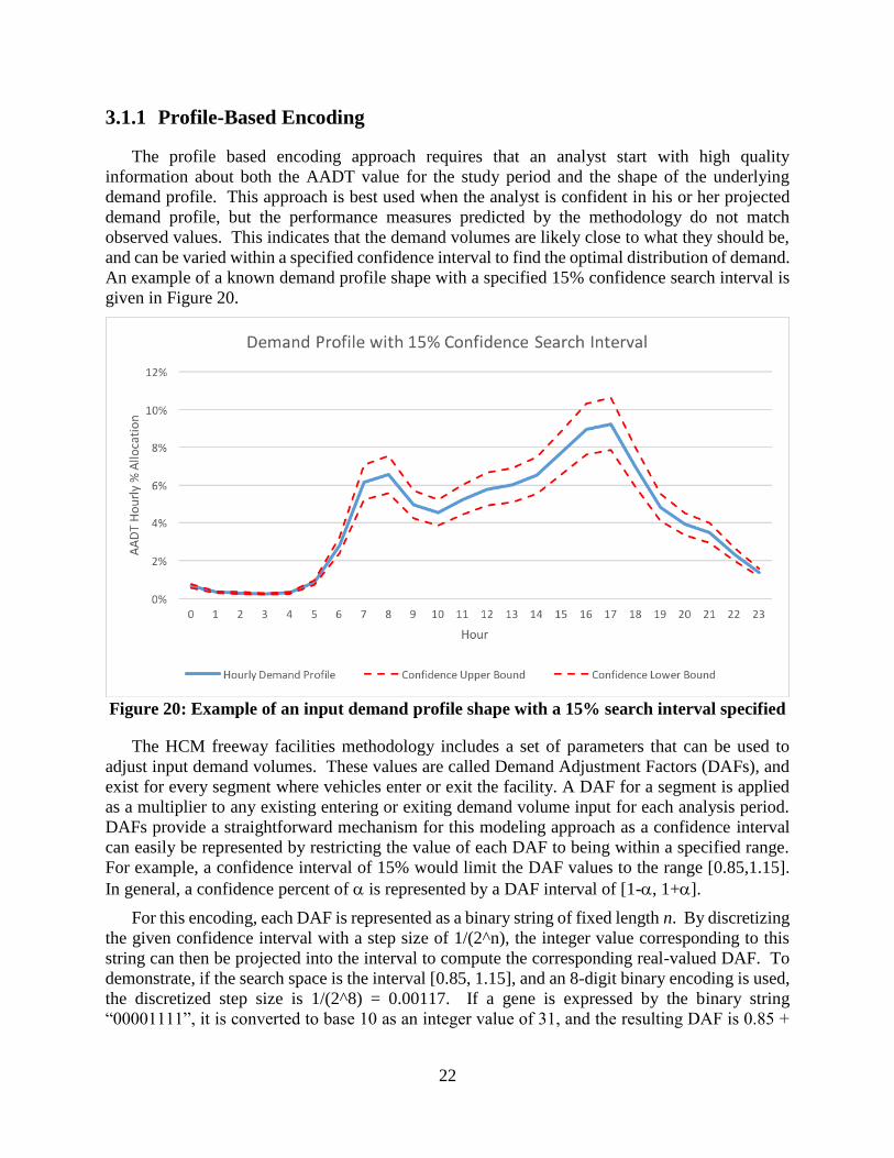
The profile based encoding approach requires that an analyst start with high quality
information about both the AADT value for the study period and the shape of the underlying
demand profile. This approach is best used when the analyst is confident in his or her projected
demand profile, but the performance measures predicted by the methodology do not match
observed values. This indicates that the demand volumes are likely close to what they should be,
and can be varied within a specified confidence interval to find the optimal distribution of demand.
An example of a known demand profile shape with a specified 15% confidence search interval is
given in Figure 20.
Figure 20: Example of an input demand profile shape with a 15% search interval specified
The HCM freeway facilities methodology includes a set of parameters that can be used to
adjust input demand volumes. These values are called Demand Adjustment Factors (DAFs), and
exist for every segment where vehicles enter or exit the facility. A DAF for a segment is applied
as a multiplier to any existing entering or exiting demand volume input for each analysis period.
DAFs provide a straightforward mechanism for this modeling approach as a confidence interval
can easily be represented by restricting the value of each DAF to being within a specified range.
For example, a confidence interval of 15% would limit the DAF values to the range [0.85,1.15].
In general, a confidence percent of is represented by a DAF interval of [1-, 1+].
For this encoding, each DAF is represented as a binary string of fixed length n. By discretizing
the given confidence interval with a step size of 1/(2^n), the integer value corresponding to this
string can then be projected into the interval to compute the corresponding real-valued DAF. To
demonstrate, if the search space is the interval [0.85, 1.15], and an 8-digit binary encoding is used,
the discretized step size is 1/(2^8) = 0.00117. If a gene is expressed by the binary string
“00001111”, it is converted to base 10 as an integer value of 31, and the resulting DAF is 0.85 +

23
(31*0.00117) = 0.97. Further, the resolution of the search space can easily be adjusted by simply
increasing or decreasing the number of binary digits considered.
3.1.2 Mixture Distribution Encoding
While an analyst often has access to reliable information regarding the magnitude and daily
behavior of demand for their facility and study period, there are still many cases where such
information is unavailable. This renders use of the approach of the previous section largely flawed,
as the process is entirely dependent on the initial guess for the shape of the profile. To circumvent
this shortcoming, this work developed a demand estimation encoding that can be used to build
viable profiles from little or no information. The approach centers on a key assumption: the daily
distribution of traffic demand can be represented by the weighted combination of n continuous
random variable distributions. The density function of the resulting mixture distribution can then
be paired with an AADT value to generate a demand profile for the study period. The probability
distribution function (PDF) of a mixture distribution is represented by Equation 1.
n
i
ii xpwxp1
)()( , where
n
i
iw1
1 (1)
In general, a mixture distribution is defined as being the weighted combination of n
independent probability distributions. Each distribution is assigned a weight wi, with all weights
summing to a value of 1. The probability density function of such a distribution is defined as the
weighted sum of the PDFs of each individual distribution, as shown in Equation 1. For the
purposes of this work, it is assumed that all random variables making up the mixture distribution
have continuous PDFs, which implies that the PDF of Equation 1 is also continuous.
A mixture distribution gives the representation near unlimited flexibility in the shape of the
resulting PDF and corresponding demand profile. To reduce the search space to a reasonable size
as well as improve convergence, assumptions can be made about the number of distributions n, as
well as the type of each. In keeping with the intuitive example mentioned above, n is always
assumed to take on a value of 3 for this research. Further, the type of the individual distributions
is limited to either being a skew-normal or a skew-Cauchy distribution. Figures Figure 21 and
Figure 22 shows examples of the variety of shapes afforded by these two distributions. However,
if for a specific facility these assumptions do not provide acceptable results, both can be altered or
relaxed back to their generalized state.

24
Figure 21: The skew normal distribution with varying values for the skewness parameter
Figure 22: The skew Cauchy distribution with varying values for the skewness parameter
25
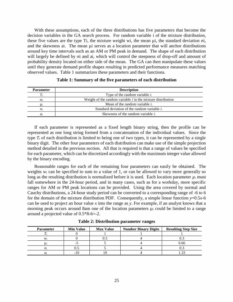
With these assumptions, each of the three distributions has five parameters that become the
decision variables in the GA search process. For random variable i of the mixture distribution,
these five values are the type Ti, the mixture weight wi, the mean µi, the standard deviation σi,
and the skewness ai. The mean µi serves as a location parameter that will anchor distributions
around key time intervals such as an AM or PM peak in demand. The shape of each distribution
will largely be defined by σi and ai, which will control the steepness of drop-off and amount of
probability density located on either side of the mean. The GA can then manipulate these values
until they generate demand profile shapes resulting in predicted performance measures matching
observed values. Table 1 summarizes these parameters and their functions.
Table 1: Summary of the five parameters of each distribution
Parameter Description
Ti Type of the random variable i.
wi Weight of the random variable i in the mixture distribution
µi Mean of the random variable i.
σi Standard deviation of the random variable i.
ai Skewness of the random variable i.
If each parameter is represented as a fixed length binary string, then the profile can be
represented as one long string formed from a concatenation of the individual values. Since the
type Ti of each distribution is limited to being one of two types, it can be represented by a single
binary digit. The other four parameters of each distribution can make use of the simple projection
method detailed in the previous section. All that is required is that a range of values be specified
for each parameter, which can be discretized accordingly with the maximum integer value allowed
by the binary encoding.
Reasonable ranges for each of the remaining four parameters can easily be obtained. The
weights wi can be specified to sum to a value of 1, or can be allowed to vary more generally so
long as the resulting distribution is normalized before it is used. Each location parameter µi must
fall somewhere in the 24-hour period, and in many cases, such as for a workday, more specific
ranges for AM or PM peak locations can be provided. Using the area covered by normal and
Cauchy distributions, a 24-hour study period can be converted to a corresponding range of -6 to 6
for the domain of the mixture distribution PDF. Consequently, a simple linear function y=0.5x-6
can be used to project an hour value x into the range as y. For example, if an analyst knows that a
morning peak occurs around 8am one of the location parameters µi could be limited to a range
around a projected value of 0.5*8-6=-2.
Table 2: Distribution parameter ranges
Parameter Min Value Max Value Number Binary Digits Resulting Step Size
Ti 0 1 1 1
wi 0 0.5 4 0.3
µi -5 5 4 0.66
σi 0.5 5 4 0.3
ai -10 10 4 1.33

26
Figure 23: String to random probability density function conversion
Table 2 and Figure 23 demonstrate the process of encoding the five decision parameters for a
single random variable into binary string. Table 2 outlines the ranges for the five parameters, and
computes the step size based on the number of binary digits of the encoding. Figure 23 explicitly
demonstrates the relationship between the binary representation and the values that shape the
probability distribution function. Building on this process, Table 3 and Figure 24 show how three
random variables are combined to create a mixture distribution representing the demand profile
for a study period.
Table 3: Parameters for each of the three random variables of the example mixture
distribution
Parameter Value Binary
T1 Normal 1
w1 0.2 0101
µ1 -2.33 0100
σ1 1.7 0100
a1 -2.02 0110
T2 Cauchy 0
w2 0.32 1001
µ2 -0.33 0111
σ2 1.0 0111
a2 1.0 1000
T3 Cauchy 0
w3 0.32 1001
µ3 1.6 1011
σ3 2.3 0110
a3 5.96 1100

27
Figure 24: Probability density functions of the full mixture distribution and the component
random variables
3.2 COMPUTATIONAL STUDIES AND RESULTS
The encodings of the previous sections were implemented into a genetic algorithm framework
built in the Java programming language. The GA framework was built alongside the FREEVAL
core computational engine, and integrated into the user interface. The following sections present
two computational experiments. The first presents a simple example in which the “ground truth”
demand is known. The second presents a case study conducted on a real world stretch of freeway
outside of Raleigh, North Carolina in which only limited information is known.
3.2.1 Simple Computational Example
This section tests the ability of the GA to calibrate the methodology for a simple example
where the underlying demand is known. This assumption of known ``ground truth" provides an
opportunity to analyze how the framework performs in a best case scenario, as opposed to jumping
directly to a real-world case study where a lack of ground truth can make it difficult to draw
conclusions about its effectiveness. For this example, there is an assumption that the values for
free flow speed and capacity are known. Both the profile-based and the n-distribution encodings
are tested and compared based on their ability to match predicted facility performance measures
to a set of target speeds.
For this case study, a basic facility was designed to be analyzed over a 24-hour study period.
The geometry of the test facility is shown in Figure 25. The facility consists of 27 half-mile
segments, with a lane-drop in the 26th segment designed to create a flow bottleneck. The facility
has a free flow speed of 65 mph, and the HCM default values for capacity are used for each
segment. The facility is assigned an unidirectional AADT value of 69,000 at the upstream
mainline entrance, which is allocated to the study period according to the 25th percentile bimodal
AM peak demand profile shown in Figure 26. The left half of Figure 27 shows the resulting speed
contour obtained from the HCM freeway facilities analysis. The contour clearly shows two

28
congestion areas, with the larger of the two occurring during the morning peak hours. This set of
speeds serves as the target data set that the GA framework will be attempt to match.
Figure 25: Geometry of the example facility. The bottleneck resulting from the lane drop
in segment 26 creates two congestion regimes over the study period.
Figure 26: Bimodal-AM Peak 25th Percentile demand profile used to allocate the AADT
over the study period
As previously noted, there is an assumption that values for all inputs other than the demand
allocation are known a priori to the analyst. For testing the calibration methodology, the GA will
be responsible for allocating the demands according to each of the two encoding approaches.
Setting the example up in this way allows for analysis to be conducted where the target
performance measures are guaranteed to be achievable with the methodology. Additionally, the
demand profile estimated by the GA framework can be compared to its underlying ground truth -
something that is generally impossible when analyzing real-world facilities.
The following two sections present the results of the using the GA framework to calibrate the
facility using both the profile-based and the n-distribution encoding. First, profile-based approach
is tested in the context where the analyst has a similar but incorrect demand allocation profile as a
starting point. Next, a 3-distribution encoding is used where it is assumed that the analyst only
knows the AADT and some basic information about the locations of congestion peaks.

29
Figure 27: Left: Speed contour obtained after performing the HCM analysis that is used as
the target data set for calibration
3.2.1.1 Results Using the Profile-Based Encoding
The first scenario assumes that the analyst starts with the average bimodal AM peak demand
profile. A comparison of the 25th percentile and average profile is shown in Figure 26.
Additionally, a unidirectional AADT value of 80,000 is initially used to allocate demands volumes
to the 15-minute analysis period intervals. The resulting speed contour predicted by the analysis
is shown on the right in Figure 27. This contour reveals a much larger congestion regime compared
to the target speeds (shown on the left), including problematic spillover beyond the boundary of
the analysis. A set of metrics is given in
Table 5 concerning the “fitness” of this initial starting point. These show that on average there
is nearly a 15 mph difference between the uncalibrated and target speeds, with some uncalibrated
speeds being more than 55 mph off.
The profile-based encoding approach is used to calibrate the demand profile of the facility
under this scenario. A confidence interval of 15\% is specified to create the search space for the
algorithm. A summary of the additional parameters for the experiment and the GA setup is given
in Table 4, and the results of five GA runs are shown in Table 5. These results show that the GA
was very successful in calibrating the facility. On average, the overall error in speeds is reduced
by 97\%, which translates to an average error of just 0.4 mph per segment per time period. While
some large individual errors still exist, an average 90th percentile error of 0.78 mph shows the GA
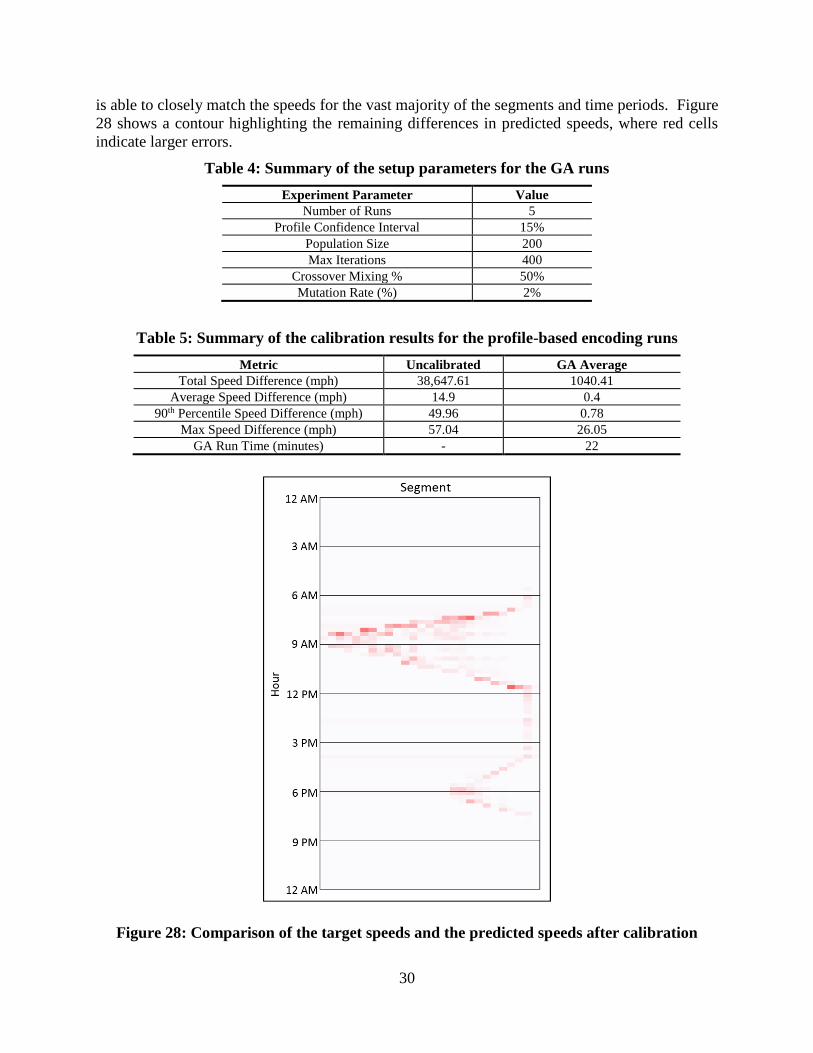
30
is able to closely match the speeds for the vast majority of the segments and time periods. Figure
28 shows a contour highlighting the remaining differences in predicted speeds, where red cells
indicate larger errors.
Table 4: Summary of the setup parameters for the GA runs
Experiment Parameter Value
Number of Runs 5
Profile Confidence Interval 15%
Population Size 200
Max Iterations 400
Crossover Mixing % 50%
Mutation Rate (%) 2%
Table 5: Summary of the calibration results for the profile-based encoding runs
Metric Uncalibrated GA Average
Total Speed Difference (mph) 38,647.61 1040.41
Average Speed Difference (mph) 14.9 0.4
90th Percentile Speed Difference (mph) 49.96 0.78
Max Speed Difference (mph) 57.04 26.05
GA Run Time (minutes) - 22
Figure 28: Comparison of the target speeds and the predicted speeds after calibration

31
Since this example is designed with the explicit goal of being able to compare estimated
demands with known ground truth demands, a deeper look can be taken at the underlying profiles
generated by the GA framework. However, unlike most other result metrics, multiple demand
profiles cannot be averaged into a single profile to gauge the effectiveness. As such, both profiles
corresponding to the best and the worst of the GA runs are shown in Figure 29. Each profile plot
shows the initial profile guess, the actual underlying profile, and the profile estimated by the GA.
While there is some noise within the generated profiles, it is clear that the GA consistently
estimated a shape much closer to that of the true profile. The improvement is especially apparent
during the AM peak where there is a near perfect reduction from the base profile to the true shape.
Much of the error that exists occurs when the methodology is in the undersaturated regime, where
speeds do not reflect the underlying demands in a one-to-one way, and additional target data (e.g.
observed throughput or volumes) would be required for further accuracy.
Figure 29: Comparison of profiles generated by the best and the worst of the GA
calibration runs, the “ground truth” profile is represented by the dotted line, while the
predicted profile is given by the solid line
3.2.2 I-540 Case Study
While the theoretical example of the previous section shows that the GA methodology can
accurately calibrate the demands for a facility using a set of target speeds, it is also important to
show that the approach is effective for real-world facilities. To accomplish this, a real-world case
study was developed based on a stretch of urban freeway on I-540 outside of Raleigh, NC. The
14.5-mile-long facility includes seven on-ramps and eight off-ramps, yielding a total of 16
(including the mainline) demand entry and exit points needing to be estimated or calibrated. The
geometry of the case study facility is given in Figure 30. The facility consists largely of three lane
segments, and the free flow speed is thought to be 75 mph. The target data speed contour, shown
in Figure 31 , was determined for a five-and-a-half-hour study period from 6:00am to 11:30am on
Tuesday, August 19th, 2014 (data collected from RITIS.org), and AADT information was gathered
from the state department of transportation (NCDOT).
Figure 30: Geometry of the I-540 westbound case study facility
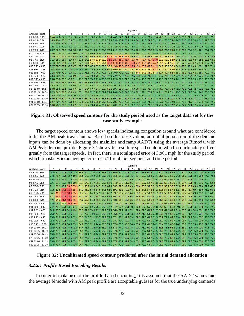
32
Figure 31: Observed speed contour for the study period used as the target data set for the
case study example
The target speed contour shows low speeds indicating congestion around what are considered
to be the AM peak travel hours. Based on this observation, an initial population of the demand
inputs can be done by allocating the mainline and ramp AADTs using the average Bimodal with
AM Peak demand profile. Figure 32 shows the resulting speed contour, which unfortunately differs
greatly from the target speeds. In fact, there is a total speed error of 3,901 mph for the study period,
which translates to an average error of 6.11 mph per segment and time period.
Figure 32: Uncalibrated speed contour predicted after the initial demand allocation
3.2.2.1 Profile-Based Encoding Results
In order to make use of the profile-based encoding, it is assumed that the AADT values and
the average bimodal with AM peak profile are acceptable guesses for the true underlying demands

33
(which are entirely unknown). Since the speeds of the initial demand allocation differ greatly from
the target data, a large confidence bandwidth of 20% is specified to define the search space for the
encoding. Five calibrations runs were performed using the GA approach based on the parameters
given in Table 6.
Table 6: Summary of the setup parameters for the profile-based GA runs
Experiment Parameter Value
Number of Runs 5
Profile Confidence Interval 20%
Population Size 200
Max Iterations 400
Crossover Mixing % 50%
Mutation Rate (%) 2%
Table 7 summarizes the results of the five calibration attempts. On average, the GA is able to
calibrate the model such that it results in a 48% reduction in total speed error. This corresponds
to an average speed difference of around 3 mph for each segment in each time period. Figure 33
shows the speed contour predicted by the best calibration attempt. While there is still a moderate
amount of error in the speeds, the contour does show congestion far more consistent with the target
data than is seen in the initial guess (see Figure 32).
Table 7: Results summary of the GA Calibration Runs
Metric Uncalibrated GA Average
Total Speed Difference (mph) 3901.5 2018.01
Average Speed Difference (mph) 6.12 3.16
90th Percentile Speed Difference (mph) 13.48 6.83
Max Speed Difference (mph) 50.31 32.75
GA Run Time (minutes) - 4.84
Figure 33: Predicted speed contour resulting from the calibration run with the lowest total
speed error

34
It is important to note that unlike the previous example, this case study is attempting to match
target speeds that may not be exactly achievable by the methodology. The reported real-world
speeds contain uncertainty in their measurement, and only provide an averaged snapshot of a
particular point in time. There is always a guarantee of some degree of error, which holds
especially true for segments and time periods where the HCM methodology reports traffic is
moving at free flow speed. Free flow speed is an input of the methodology and is assumed to be
one constant value for all vehicles. Additionally, one of its primary uses is to serve as an upper
bound on predicted speed. However, in real-world conditions, free flow speed will vary from
driver to driver independent of the demand volume, even when demands are far below capacity.
With this in mind, the calibration shown in Figure 33 can be considered a success as it successfully
removes the incorrect congestion regime of the initially estimated contour, and now predicts a
speed pattern largely consistent with the target data.
Taking a deeper look at the remaining errors in speed, and breaking them down by speed
regime provides additional insight into the calibration process. Table 8 shows a breakdown of the
average absolute speed error of the three regimes. The first regime considers any segment and time
period combination in which the target speed is greater than 55 mph. The second speed regime
considers a target speed less than 55mph, and the final regime considers a target speed of less than
45 mph. It is clear that for the uncalibrated facility, the errors escalate severely as the target speed
drops, with mean errors of 17 mph for the second speed regime and 22 mph for the third speed
regime. On the other hand, the first attempt at calibration, which uses an unweighted objective
function and whose overall results are discussed above, shows a marked improvement. The error
breakdown by speed regime is shown in the middle row of Table 8, and the errors for the lower
speed regimes drop by 50% and 60%, respectively.
Table 8: Breakdown of the mean absolute speed error of each segment in each time period
for three speed regimes using the profile-based encoding
Speed Regime Overall >55 <55 <45
Uncalibrated Avg Absolute Speed Error (mph) 6.11 5.31 17.22 21.83
Calibrated (Unweighted) Avg Absolute Speed Error (mph) 3.16 2.81 8.07 8.79
Calibrated (Weighted) Avg Absolute Speed Error (mph) 4.48 4.52 3.95 4.01
In order to improve the calibration accuracy further, the fitness function is altered such that
errors occurring when the target speed is lower are weighted more heavily. Any number of
weightings can be used, but a simple weighting scheme for the objective is given in Equation 2.
This serves to weight errors where the target speed is less than 55 mph twenty times more
important than when the target speed is greater than 55 mph. A value of 20 is chosen because the
speed regime cutoff of 55 mph is 20 less than the facility free flow speed of 75 mph. Another 5
runs of the calibration GA are made using this new objective function, and the breakdown of the
average speed error is given in the final row of Table 8. While the overall average speed error is
higher, there is sizable improvement in the predicted speeds for the lower speed regimes, where
the average error fell by more than 50% from the unweighted calibration. From this it can be seen
that making use of a weighted objective function such as that in Equation 2 can be very helpful to
tailor the focus of a calibration. More focused calibration such as this can be particularly useful
when the number of periods with low speeds is outnumbered by periods in which speeds are
essentially at free flown conditions.

35
N
i
P
p pipipi vv1 1 ,,, , where
55 if 1
55 if 20
,
,
,
pi
pi
pi v
v (2)
3.2.2.2 3-Distribution Encoding Results
For a second attempt at calibrating the I-540 facility using the GA approach, a 3-distribution
encoding approach is utilized and the results are compared to those obtained using the profile-
based encoding. Tables Table 9 and
Table 10 provide the parameters used for the GA for a demand estimation approach using a 3-
distribution encoding and the unweighted objective function of Equation 2. The ranges specified
for the mixture distribution are also mostly the same as with previous examples. However, for this
case study, two of the location parameters are left unconstrained (within the 24-hour daily limit),
while the target data is used to restrict the location of one of the random variables. Figure 31
shows that the congestion falls entirely between 7:00am and 10:00am, and that range is used to
limit the value of µ1.
Table 9: Summary of the setup parameters for the 3-distribution encoding GA runs
Experiment Parameter Value
Number of Runs 5
Population Size 400
Max Iterations 200
Crossover Mixing % 50%
Mutation Rate (%) 2%
Table 10: Summary of the distribution parameters for the 3-distribution encoding
Distribution Parameter Symbol Range
Weight wi 0.05,0.5
Mean 1 µ1 7:00am, 10:00am
Mean 2 µ2 12:00am, 11:59pm
Mean 3 µ3 12:00am, 11:59pm
Standard Deviation σi 0.5,5.0
Skewness ai -10,10
A summary of the results of the experiment is given in Table 11, and the contour predicted
by the estimated demands for the best run is shown in
Figure 34. The contour shows a patch of lowered speeds from 7am to 9am, with a shape
roughly matching that of the target speed data, indicating a successful calibration. Further, the
average error of 3.12 mph is slightly less than that obtained with the profile-based calibration
approach. This implies that for a situation with this little of quality input data available, estimating
the demand profile using a 3-distribution approach is likely the better alternative.

36
Table 11: Results summary of the GA Calibration Runs
Metric Uncalibrated GA Average
Total Speed Difference (mph) 3901.5 1991.8
Average Speed Difference (mph) 6.12 3.12
90th Percentile Speed Difference (mph) 13.48 6.27
Max Speed Difference (mph) 50.31 28.06
GA Run Time (minutes) - 8.3
Figure 34: Speed contour of the calibrated facility with the lowest total speed error
Table 12 provides a breakdown of the error for the five calibration runs discussed above with
an unweighted objective, as well as for five additional calibration runs made with the same 3-
distribution encoding and the regime-weighted objective of Equation 2. The breakdown for the
runs with the unweighted objective again shows that the GA was significantly less accurate in
matching the lower speed regimes than the higher speed regimes. For the calibration attempts
using the weighted objective function, the distribution of error is much more even. There is a large
reduction in the average speed error for both of the lower speed regimes, with the lowest regime
seeing nearly a 70\% improvement. This strongly reinforces the usefulness of a weighted objective
function when the number of periods with high target speeds outnumbers those with lower target
speeds.
Table 12: Breakdown of the mean absolute speed error of each segment in each time period
for three speed regimes of the 3-distribution encoding calibration
Speed Regime Overall >55 <55 <45
Uncalibrated Avg Absolute Speed Error (mph) 6.11 5.31 17.22 21.83
Calibrated (Unweighted) Avg Absolute Speed Error (mph) 3.12 2.71 9.08 10.65
Calibrated (Weighted) Avg Absolute Speed Error (mph) 3.56 3.52 4.48 3.35
37
4.0 FREEVAL CALIBRATION
4.1 IMPORTANCE OF FREEVAL CALIBRATION
The process of facility calibration is a foundational aspect of using the HCM methodology and
a critical step of model creation preceding all analyses. Model calibration is essential because any
analysis that uses the HCM methodology hinges on the core model correctly representing daily
recurring congestion conditions. In fact, modeling existing real-world conditions for a single
representative day is the first step for using the methodology to conduct reliability and active traffic
management analyses. This requirement necessitates that every model must be calibrated to match
a set of target real-world conditions. The manual's current guidance concerning calibration is very
limited, and the process often presents a major barrier to entry for the methodology.
Much of the challenge of the calibration process stems from the fact that each model requires
a large number of inputs, with even moderate sized models requiring the input and adjustment of
thousands of individual parameters. Further, many of the critical inputs are difficult to measure
under real-world conditions. Calibration of both input demand volumes and capacity parameters
is vitally important as the driving force of the methodology is the relationship between demand
volumes and segment throughput capacities. However, vehicle demand volumes are largely
unknown under real world conditions and are essentially impossible to measure when traffic flow
is congested. The manual does provide default estimates for the key capacity parameters, but these
should ideally be adjusted in conjunction with demand volumes for each specific facility location.
4.2 INTEGER PROGRAMMING APPROACH
While both the freeway facilities method of the HCM and the original CTM can be solved
efficiently by iterating through the flow equations, this provides little advantage when attempting
to calibrate a facility. Further, this straightforward approach to the analysis is limited in that the
unknowns are fixed and the solutions only provide a specific set of performance measures. This
yields little real insight into the interplay between variables and sensitivities of each respective
model. In order to gain better insight into the workings of the methods, it is thus desirable to
formulate them as optimization problems. Much work has already been done to model the CTM
using mathematical programming frameworks, but little has been done for the HCM freeways
methodology. These approaches have largely used linear programming, integer programming, and
nonlinear programming. The CTM was first formulated as linear program (LP) by Ziliaskopoulos
(2000) where he defined the System Optimum Dynamic Traffic Assignment (SO DTA) problem.
Aghdashi et al. (2013) developed a linear programming model to compute optimal ramp metering
strategies based on the undersaturated equations.
This work formulates the oversaturated methodology as a Mixed Integer Linear Program
(MILP). The unique ability of the MILP formulation to allow for ``forward", ``backward", or
``inside-out" analysis is explored in an effort to gain better insight into the benefits and limitations
of the model.

38
4.2.1 Formulation of the MILP Model
This work focuses solely on the oversaturated portion of the freeways facility methodology.
In part, this is due to the undersaturated algorithm being relatively computationally simple and
efficient, and largely because it is of limited usefulness in the context of facility calibration. In
cases where the facility is undersaturated, it is known that all demand can and is being met, and
thus the demand is simply equivalent to the observed flows. Further, it should be noted that the
undersaturated conditions can be analyzed using the oversaturated equations. The methodology
as presented in the HCM does not do this in order to eliminate unnecessary computational efforts
and costs.
As soon as the demand exceeds capacity on a segment of the facility, the oversaturated
procedure is utilized. The oversaturated equations evaluate the facility by computing flows for
each node, starting at the first upstream node and moving down the facility. Flows at each node
consist of three quantities, mainline flow (MF), on-ramp flow (ONRF), and off-ramp flow (OFRF).
Segment flows (SF) are calculated for each intermediate segment, though each can easily be
associated with a node to simplify the computations. Figure 35 shows how mainline and segment
flows interact at merge and diverge segments.
Figure 35: Example of the mainline flow (MF) and the segment flow (SF) calculations with
on-ramps and off-ramps
The bulk of the computations of the methodology involve the computation of these flows.
Flows for the mainline and ramps are limited both by the input flow desiring to travel through the
node, as well as the output flow that can be allowed based on available capacity, adjacent ramp
flow, and queue conditions. These computations contain nonlinearities in the form of “min”
functions that force the flow to be the minimum of input and output. As an illustration, the
following paragraph will briefly discuss the computation of mainline flow at a node, and similar
methodology is contained within the oversaturated equations for computing on-ramp and off-ramp
flows.
Computing mainline flow at a node consists of computing the mainline input (MI) wishing to
travel through the node, as well as computing a number of quantities that can limit the output flow
through the node due to the presence of a ramp at the node, or a queue created by a downstream
bottleneck. Mainline input at a node is the sum of the mainline flow and on-ramp flow coming
from the node immediately upstream, minus any off-ramp flows of the current node. If a queue
exists, mainline input also includes any unserved vehicles (UV) stored on the upstream segment.
Mainline output is limited by three quantities accounting for turbulence due to merging on-ramp
flows, queue accumulation from a downstream bottleneck, and queue dispersion from a

39
downstream bottleneck, respectively. Mainline output is also limited by the capacity of each of
the segments to which it is adjacent. Consequently, the equation to determine mainline flow is
presented in the methodology as:
),,1(
),,(
),,(3
),,(2
),,(1
),,(
),,(
ptiSC
ptiSC
ptiMO
ptiMO
ptiMO
ptiMI
ptiMF (3)
While it is sometimes possible to directly linearize an equation such as this with a group of “≤”
inequalities, it is unfortunately generally not the case for this model. Depending on the choice of
objective functions and the rest of the constraints, simply using inequalities can lead to a
phenomenon known as “holding back flows.” For example, since this approach is seeking to
optimize the system as a whole, flows may be artificially held back from progressing through a
node when it benefits this system. This can occur with groups of “≤” inequalities since the flow
is only required to be less than both the input and the output, but not exactly the minimum of the
two. This type of behavior is highly unrealistic and it is generally accepted that any vehicle
traveling through a facility will seek to minimize its own travel time, even at the cost of the
performance of the facility as a whole. This type of condition is referred to as the User Optimum
(UO) or User Equilibrium (UE) condition. Thus the MILP formulated will make use of binary
integer variables in order to model these “min” functions in an exact manner.
The MILP is formulated by using each equation of the oversaturated methodology as a model
constraint. The equations are formulated as constraints by using them directly as linear equalities
when possible, or by converting them to sets of linear inequalities when necessary. These
constraints are then paired with an objective function that minimizes the difference between
predicted and target performance measures in order to determine the optimal set of decision
variables. In this case, the decision variables are previously determined by the analyst, and are the
input parameters (e.g. demand volumes, capacity adjustments) for which the analyst wishes to
calibrate the model.
4.2.2 Minimum and Maximum Relationships as Constraints
While linear programming is a very powerful tool, it does have a strict limitation in that it can
only model expressions which can be formulated as sets of linear equalities and inequalities. This
raised a major issue for this work as many of the most important equations of the HCM
methodology require taking the minimum or maximum of a set of values. Consequently, in order
to handle min/max constraints, a pure LP model must be expanded to include binary integer
decision variables, allowing the min/max relationships to be accurately modeled. The following
example shows how a simple “min” relationship can be modeled as a set of linear inequalities
through the use of binary variables.
Consider the statement C=min{A,B}. In practice, this statement is essentially an “If-Then”
conditional: If A < B, then C=A, and a constraint of C-A=0 must be enforced, and if A>B, then
C=B and the constraint C-B=0 must be enforced. By adding a binary decision variable i, and a
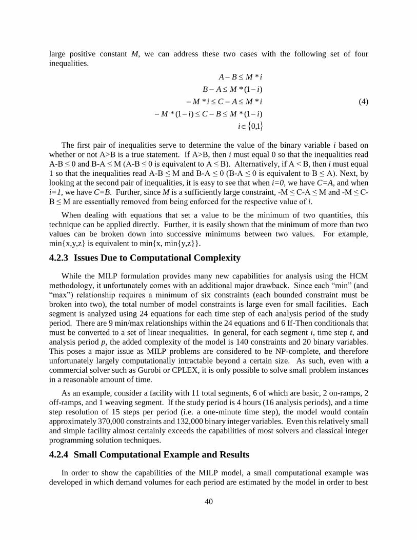
40
large positive constant M, we can address these two cases with the following set of four
inequalities.
1,0
)1(*)1(*
**
)1(*
*
i
iMBCiM
iMACiM
iMAB
iMBA
(4)
The first pair of inequalities serve to determine the value of the binary variable i based on
whether or not A>B is a true statement. If A>B, then i must equal 0 so that the inequalities read
A-B ≤ 0 and B-A ≤ M (A-B ≤ 0 is equivalent to A ≤ B). Alternatively, if A < B, then i must equal
1 so that the inequalities read A-B ≤ M and B-A ≤ 0 (B-A ≤ 0 is equivalent to B ≤ A). Next, by
looking at the second pair of inequalities, it is easy to see that when i=0, we have C=A, and when
i=1, we have C=B. Further, since M is a sufficiently large constraint, -M ≤ C-A ≤ M and -M ≤ C-
B ≤ M are essentially removed from being enforced for the respective value of i.
When dealing with equations that set a value to be the minimum of two quantities, this
technique can be applied directly. Further, it is easily shown that the minimum of more than two
values can be broken down into successive minimums between two values. For example,
min{x,y,z} is equivalent to min{x, min{y,z}}.
4.2.3 Issues Due to Computational Complexity
While the MILP formulation provides many new capabilities for analysis using the HCM
methodology, it unfortunately comes with an additional major drawback. Since each “min” (and
“max”) relationship requires a minimum of six constraints (each bounded constraint must be
broken into two), the total number of model constraints is large even for small facilities. Each
segment is analyzed using 24 equations for each time step of each analysis period of the study
period. There are 9 min/max relationships within the 24 equations and 6 If-Then conditionals that
must be converted to a set of linear inequalities. In general, for each segment i, time step t, and
analysis period p, the added complexity of the model is 140 constraints and 20 binary variables.
This poses a major issue as MILP problems are considered to be NP-complete, and therefore
unfortunately largely computationally intractable beyond a certain size. As such, even with a
commercial solver such as Gurobi or CPLEX, it is only possible to solve small problem instances
in a reasonable amount of time.
As an example, consider a facility with 11 total segments, 6 of which are basic, 2 on-ramps, 2
off-ramps, and 1 weaving segment. If the study period is 4 hours (16 analysis periods), and a time
step resolution of 15 steps per period (i.e. a one-minute time step), the model would contain
approximately 370,000 constraints and 132,000 binary integer variables. Even this relatively small
and simple facility almost certainly exceeds the capabilities of most solvers and classical integer
programming solution techniques.
4.2.4 Small Computational Example and Results
In order to show the capabilities of the MILP model, a small computational example was
developed in which demand volumes for each period are estimated by the model in order to best
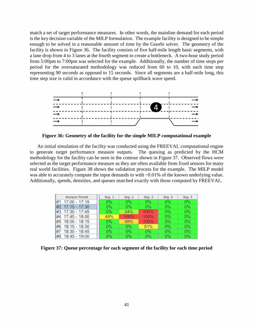
41
match a set of target performance measures. In other words, the mainline demand for each period
is the key decision variable of the MILP formulation. The example facility is designed to be simple
enough to be solved in a reasonable amount of time by the Guorbi solver. The geometry of the
facility is shown in Figure 36. The facility consists of five half-mile length basic segments, with
a lane drop from 4 to 3 lanes at the fourth segment to create a bottleneck. A two-hour study period
from 5:00pm to 7:00pm was selected for the example. Additionally, the number of time steps per
period for the oversaturated methodology was reduced from 60 to 10, with each time step
representing 90 seconds as opposed to 15 seconds. Since all segments are a half-mile long, this
time step size is valid in accordance with the queue spillback wave speed.
Figure 36: Geometry of the facility for the simple MILP computational example
An initial simulation of the facility was conducted using the FREEVAL computational engine
to generate target performance measure outputs. The queuing as predicted by the HCM
methodology for the facility can be seen in the contour shown in Figure 37. Observed flows were
selected as the target performance measure as they are often available from fixed sensors for many
real world facilities. Figure 38 shows the validation process for the example. The MILP model
was able to accurately compute the input demands to with ~0.01% of the known underlying value.
Additionally, speeds, densities, and queues matched exactly with those computed by FREEVAL.
Figure 37: Queue percentage for each segment of the facility for each time period

42
Figure 38: Validation process for the predicted demands computed with the MILP model
While this example demonstrates the power of the approach to accurately estimate inputs based
on a set of target performance measures, it also highlights its limitations due to the inherent
computational complexity of MILP models. Even for an example this small, there were over
26,000 constraints and over 23,000 variables, 10,000 of which were binary variables. While this
problem can be solved quickly in about 10.5 seconds, each additional segment, especially ramp
segments, increases the computational burden exponentially, quickly moving the model to the
realm of intractability with today’s computers.
4.3 A GENETIC ALGORITHM APPROACH
This genetic algorithm framework of this section expands upon the demand estimation
approach by adding three key capacity parameters into the existing calibration framework. New
genetic encodings for the inputs are developed that allow the metaheuristic to consider pre-
breakdown capacity adjustments, the queue discharge flow rate, and the facility-wide jam density
alongside demand volumes. These three capacity parameters are important to incorporate as each
controls aspects of breakdown occurrence, queue formation and recovery speeds, and overall
queue size in a unique way. The resulting framework consists of a two-phase calibration process.
During the first phase, the GA adjusts demand volumes and the queue discharge rate, while at the
second phase the GA manipulates the jam density and bottleneck segment pre-breakdown capacity
adjustments. Further, unlike the initial work, this expanded approach utilizes an updated objective
function that considers errors in both facility travel times and individual segment speeds.
4.3.1 Genetic Algorithm Overview
Metaheuristic approaches are often employed for problems in which the underlying
mathematical relationships of a system are poorly understood or prohibitively complex. Unlike
classical
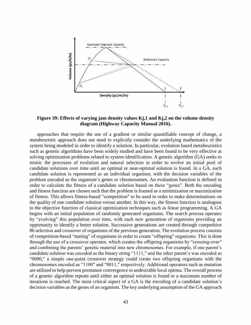
43
Figure 39: Effects of varying jam density values Kj,1 and Kj,2 on the volume density
diagram (Highway Capacity Manual 2016).
approaches that require the use of a gradient or similar quantifiable concept of change, a
metaheuristic approach does not need to explicitly consider the underlying mathematics of the
system being modeled in order to identify a solution. In particular, evolution based metaheuristics
such as genetic algorithms have been widely studied and have been found to be very effective at
solving optimization problems related to system identification. A genetic algorithm (GA) seeks to
mimic the processes of evolution and natural selection in order to evolve an initial pool of
candidate solutions over time until an optimal or near-optimal solution is found. In a GA, each
candidate solution is represented as an individual organism, with the decision variables of the
problem encoded as the organism’s genes or chromosomes. An evaluation function is defined in
order to calculate the fitness of a candidate solution based on these “genes". Both the encoding
and fitness function are chosen such that the problem is framed as a minimization or maximization
of fitness. This allows fitness-based “competition" to be used in order to make determinations on
the quality of one candidate solution versus another. In this way, the fitness function is analogous
to the objective function of classical optimization techniques such as linear programming. A GA
begins with an initial population of randomly generated organisms. The search process operates
by “evolving" this population over time, with each new generation of organisms providing an
opportunity to identify a better solution. Successive generations are created through competitive
86 selection and crossover of organisms of the previous generation. The evolution process consists
of competition-based “mating" of organisms in order to create “offspring" organisms. This is done
through the use of a crossover operator, which creates the offspring organisms by “crossing-over"
and combining the parents’ genetic material into new chromosomes. For example, if one parent’s
candidate solution was encoded as the binary string “1111," and the other parent’s was encoded as
“0000," a simple one-point crossover strategy could create two offspring organisms with the
chromosomes encoded as “1100" and “0011," respectively. Additional operators such as mutation
are utilized to help prevent premature convergence to undesirable local optima. The overall process
of a genetic algorithm repeats until either an optimal solution is found or a maximum number of
iterations is reached. The most critical aspect of a GA is the encoding of a candidate solution’s
decision variables as the genes of an organism. The key underlying assumption of the GA approach

44
is that high-quality solutions contain common “building blocks" found in the encoded genes of the
organisms (Mitchell, 1998). Maintaining these blocks within a population of organisms, and
combining them with other “good" blocks should then theoretically lead to the discovery of better
solutions. Blocks are combined through the use of a crossover operator representing mating and
reproduction of organisms. This process produces a number of “offspring" organisms each
containing parts of each parent’s genetic material and consequently the encoded decision variable
values. While real-valued encodings are occasionally used, most encodings consist of some type
of binary representation of the solution. This allows for a straightforward realization of genetic
building blocks (e.g. small binary patterns such as “010" or “110"), and provides a simple notion
of sharing genetic material through exchanging binary digits. In most cases in which a
metaheuristic approach such as a GA is necessary to solve a problem, the solution space is likely
to be highly nonlinear, nonconvex, and discontinuous. This makes it extremely difficult for any
search process to directly or smoothly move towards a globally optimal solution. Thus, most GA
implementations make use of at least one additional operator to guard against premature
convergence to locally optimal solutions. The most common of these operators is the mutation
operator, which randomly alters an organism’s individual genes or chromosomes in order to
introduce additional genetic diversity into the population.
4.3.2 Unifying Demand and Capacity Calibration
Overall, there are three key aspects of capacity that should be considered when calibrating an
HCM freeway facilities model, each of which affects the predicted performance measures in a
different manner. First, pre-breakdown bottleneck capacity adjustments determine the demand 87
level at which breakdowns occur, and have inverse effects on the shockwave formation and
recovery speeds. Second, a reduced queue discharge rate via a capacity drop factor models a known
realworld phenomenon and provides an additional control on the breakdown shockwave formation
and recovery speeds that only affects conditions post-breakdown. Lastly, the jam density of the
facility controls the length of any queues that form, which is reflected in variations in the speeds
of individual segments in and around the vehicle queue. As previously mentioned, a genetic
algorithm metaheuristic approach was developed to automate the process of demand estimation
and adjustment. The approach is able to estimate new or adjust existing demand volume inputs
such that the performance predicted by the methodology more accurately matched that of a set of
target real-world conditions. While it proved to be an improvement over the current trial and error
process, its focus only on demand left it with some inherent limitations. On its own, demand
calibration is best suited for matching observed throughput values and travel times. This may be
sufficient for some facilities, but in general, and especially when calibrating for individual segment
speeds, it is better served when complemented with capacity calibration. By incorporating capacity
parameters that control additional relevant aspects of congestion analysis (e.g., breakdown
occurrence, formation speed, queue length, and breakdown recovery), the power and flexibility of
the system identification framework can be maximized. The proposed framework consists of two-
stage approach of successive calibration instances, each of which operates on a different set of
variables during the GA search process. The first round of calibration focuses on demand
estimation, and incorporates the capacity drop factor alongside the demand volume input variables.
The second round utilizes the determined values for these inputs, and operates instead on the pre-
breakdown bottleneck adjustments and the jam density. The objective function for both instances
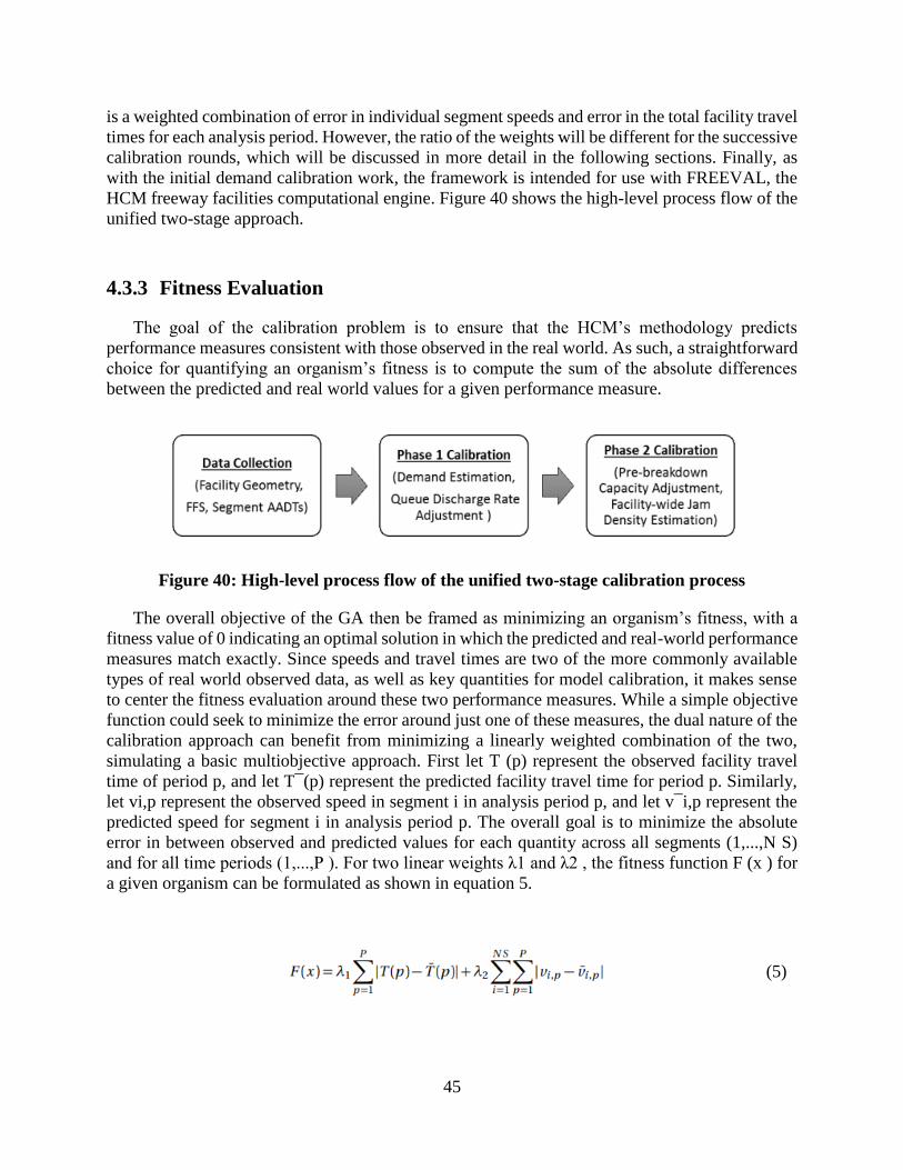
45
is a weighted combination of error in individual segment speeds and error in the total facility travel
times for each analysis period. However, the ratio of the weights will be different for the successive
calibration rounds, which will be discussed in more detail in the following sections. Finally, as
with the initial demand calibration work, the framework is intended for use with FREEVAL, the
HCM freeway facilities computational engine. Figure 40 shows the high-level process flow of the
unified two-stage approach.
4.3.3 Fitness Evaluation
The goal of the calibration problem is to ensure that the HCM’s methodology predicts
performance measures consistent with those observed in the real world. As such, a straightforward
choice for quantifying an organism’s fitness is to compute the sum of the absolute differences
between the predicted and real world values for a given performance measure.
Figure 40: High-level process flow of the unified two-stage calibration process
The overall objective of the GA then be framed as minimizing an organism’s fitness, with a
fitness value of 0 indicating an optimal solution in which the predicted and real-world performance
measures match exactly. Since speeds and travel times are two of the more commonly available
types of real world observed data, as well as key quantities for model calibration, it makes sense
to center the fitness evaluation around these two performance measures. While a simple objective
function could seek to minimize the error around just one of these measures, the dual nature of the
calibration approach can benefit from minimizing a linearly weighted combination of the two,
simulating a basic multiobjective approach. First let T (p) represent the observed facility travel
time of period p, and let T¯(p) represent the predicted facility travel time for period p. Similarly,
let vi,p represent the observed speed in segment i in analysis period p, and let v¯i,p represent the
predicted speed for segment i in analysis period p. The overall goal is to minimize the absolute
error in between observed and predicted values for each quantity across all segments (1,...,N S)
and for all time periods (1,...,P ). For two linear weights λ1 and λ2 , the fitness function F (x ) for
a given organism can be formulated as shown in equation 5.
(5)

46
While this represents the fitness function in its simplest form, it can be modified in a near
endless number of ways and tailored to a specific goal or application. For example, the work
developing the demand estimation framework found that it was beneficial to weight errors
occurring where targets speed are lower more heavily than those occurring where the target speeds
are higher. There are a variety of ways to do this, but a simple linear piecewise weighting scheme
was proposed in the demand estimation work that achieved satisfactory results. In this scheme,
errors where the target speed is less than 55 mph are weighted as much as twenty times more
heavily than where the target speed is greater than 55 mph. This allows the GA to focus on the
replicating the congested conditions, as opposed to trying to perfectly match free flow speeds in
uncongested periods. While 89 free flow speed is a constant value in the HCM methodology, it
can fluctuate widely in the real world depending on the type of driver (e.g. one who speeds versus
one who strictly obeys the speed limit) passing through the observation zone in a given time period.
Thus the fitness function can be reformulated with this modification as shown in equation set 6.
In addition to allowing the objective function to consider multiple performance measures, the
weights λ1 and λ2 serve an additional purpose for the two-stage calibration process. They allow
the focus of the optimization to be shifted between the two quantities based on the phase of the
calibration process. The first phase of the calibration process centers on demand estimation, and
hence should place a heavier weight on matching the target facility travel times. Alternatively, the
second phase of the calibration process centers on pre-breakdown capacity adjustments and jam
density, and matching individual segments speeds should be a higher priority and given a heavier
weight. The exact ratio of the weights can be adjusted for each particular calibration instance, but
a simple two-to-one ratio can serve as a default starting point.
4.3.4 Genetic Encoding of the Capacity Calibration Parameters
The GA framework of the original demand calibration work requires that all decision variables
be represented as a string (or strings) of binary digits. As such, a binary encoding process
analogous to that of the profile based demand adjustments is used to incorporate capacity
calibration parameters into the existing framework. This type of encoding necessitates an
assumption of a known range of feasible values for each parameter, which requires that both a
minimum and a maximum possible value be specified. The interval created by this range can then
be discretized using the maximum integer value allowed by the number of binary digits of the
encoding. In this way, the binary value of a gene will represent an integer value, which can then
be projected into the discretized search space. To demonstrate, if the search space for a pre-
(6)

47
breakdown CAF is the interval [0.7,1.01], and an 5-digit binary encoding is used, the range is
discretized into 31 intervals, which gives a step size of (1.010.70)/(2 5 − 1) = 3.1/31 = 0.01
(projection into the range is inclusive, hence why there are 2 5 − 1 = 31 intervals as opposed to 2
5 = 32). For a gene expressed by the binary string “010100", it 90 is converted to base 10 as an
integer value of 20, and the resulting CAF is 0.7 + (20 ∗ 0.01) = 0.90 (a simplified range is used
for demonstration purposes). Analogous approaches are used to encode and project both the
capacity drop factor and the facility-wide jam density. The specified allowable range for each
parameter can vary for each facility and should be chosen using the analyst’s judgment and
knowledge of the facility. However, any range should not be too large. For example, pre-
breakdown CAFs indicating a drop in capacity of 30% or more are likely to be unrealistic and may
indicate that other inputs of the methodology need to be adjusted. Table 13 shows a set of
recommended ranges for each of the three parameter types. It should also be noted that the number
of binary digits can be varied to increase or decrease the resolution of the CAF search space. For
example, a 5-digit binary encoding divides the search interval into 2 5 = 32 values, while a 16-
digit binary encoding divides the interval into 65,536 values.
Table 13: Recommended ranges for the capacity calibration parameters
With a binary representation for each parameter defined, the capacity parameters next need to
be incorporated into the GA framework. This requires adding the capacity drop factor to the
existing demand calibration process, and creating an additional process for estimating the pre-
breakdown capacity adjustments and the facility-wide jam density. Since the demand calibration
piece uses uniform crossover and mutation, both of which consider individual binary digits
independently, the capacity drop factor can be calibrated in conjunction with demand by simply
appending its binary representation to the encoded string of demand values or adjustments. On the
other hand, since the framework now functions as a two-stage process, an additional encoding
must be utilized for the set of pre-breakdown CAFs and the jam density. In a freeway facilities
analysis, each individual segment of a facility has a representative capacity value and a
corresponding CAF. This research assumes that capacity of a segment is fixed over time, and thus
the number of CAF decision variables considered is equal to the number of segments. The capacity
drop factor is considered to be a facility-wide value, and hence constitutes one decision variable.
For a facility with NS segments, the set of NS CAF binary encodings are then concatenated into a
single binary string. This provides a simpler (albeit analogous) representation as opposed 91 to
working with an array of binary strings. Additionally, the binary encoding of the jam density can
simply be appended to the end of the single string representation, without altering how GA
operators approach it beyond extending its length. Figure 41 demonstrates the process of encoding
a set of three pre-breakdown capacity adjustments and the facility-wide jam density into a single
binary string.

48
Table 14: Parameter minimum values and step sizes for the encoding example
Figure 41: Example of encoding three pre-breakdown CAFs and the facility-wide jam
density into binary strings based on the values of Table 14
As a final note on pre-breakdown capacity adjustment factors, this approach initially extends
their use to all segments, as opposed to just at bottleneck segments as proposed in the HCM’s
calibration procedure. The reason for this is two-fold. First, this enables the framework to make
small adjustments to segment capacities along the entire facility as the default estimates may be
slightly off. However, and more importantly, the second reason is that there is uncertainty in the
location of a bottleneck, and its location is likely relatively unknown for an uncalibrated facility.
By allowing the GA metaheuristic to adjust the CAFs for every segment, it gives it the freedom to
identify bottleneck location(s) while also determining the magnitude of the capacity adjustment(s).
Further, while the GA may in some instances adjust capacities when it has no effect on
performance measures 92 (e.g., when demand is well below capacity), a simple post-processing
check can be employed to replace these adjustments with an unadjusted value of 1.0.
4.3.5 Selection and Crossover
The primary drivers of the evolutionary process of a GA are the selection and crossover
operators. The selection operator is used to choose the two organisms (candidate parameter
adjustments in our case) that will undergo crossover in order to produce new offspring organisms.
There are a number of ways to implement the selection process including random selection,
roulette wheel selection, and tournament selection. This research makes use of a simple k-
tournament selection strategy in which k solutions are randomly picked from the current
generation, and the one with the best (lowest) fitness is selected to be a parent. This process is
repeated twice to determine the two parent organisms to undergo crossover. The value of k can be
varied to improve the convergence rate of the GA. As with selection, there are a variety of
crossover strategies and a vast amount of research conducted in regards to how these strategies
impact final solution quality and the speed of convergence. Three commonly used crossover
strategies were implemented and tested as part of this research. These included a one and two point

49
crossovers, as well as uniform crossover. Figure 42 demonstrates each of the three crossover
strategies. However, initial testing indicated that the uniform crossover strategy was by far the
most effective. Using this strategy, a random number is generated uniformly between 0 and 1 for
each binary digit of the encoding. If the generated value is less than a pre-specified mixing
percentage (e.g. 0.5 would indicate 50% mixing), the binary digit is swapped between the two
strings. As such, for the case study of the subsequent section, a uniform crossover strategy was
always used for the Phase 2 capacity calibration process.
4.3.6 Mutation
A uniform mutation strategy was implemented for use in the bottleneck capacity calibration
GA framework to help prevent premature convergence to a locally optimal solution. As its name
would suggest, a uniform mutation strategy is very similar to the previously described uniform
crossover strategy. However, unlike crossover, uniform mutation operates just on a single set of
genes in order to randomly introduce changes such that a diverse population of candidate solutions
is maintained. Further, instead of a mixing percentage hovering around 50%, mutation of
individual genes (e.g., binary digits) is generally specified to occur at a much lower frequency,
known as the mutation rate. During the mutation process for a binary string encoding, a random
number is again generated 93
Figure 42: Demonstration of three common crossover operators
uniformly between 0 and 1 for each binary digit. If the number is less than the specified
mutation rate, the corresponding binary digit is flipped to its binary alternative. Specifically, a 0
becomes a 1, and a 1 becomes a 0. The optimal mutation rate varies for each specific problem, but
research has generally shown that for binary GA encodings, a rate of 0.02 to 0.05 has the most
beneficial effect on convergence and final solution quality (Mitchell, 1998).

50
4.3.7 Computational Experiments and Numerical Results
A case study for testing the approach with real word data was developed for analysis based on
a section of I-540 outside of Raleigh, NC. The goal of the case study is to produce a calibrated
model by estimating the demand volume inputs and adjusting the core capacity parameters using
the genetic algorithm framework. The facility consists of 14.5 miles of largely three-lane urban
freeway in the westbound direction, including seven on-ramp segments and eight off-ramp
segments. The facility as modeled using the HCM methodology is shown in Figure 43. The facility
was then populated with initial demand input values based on AADT estimates available through
the North Carolina Department of Transportation and combined with a best estimate of the local
hourly demand behavior for the study period (North Carolina Department of Transportation,
2016).
Figure 43: HCM segmentation of 14.5-mile section of I-540 westbound near Raleigh, NC
A set of representative speeds for a five-and-a-half-hour study period between 6:00am and
11:30 am on a Tuesday in August 2014 was collected from RITIS.org and are shown in the top
contour of Figure 44 (Maryland CATT Lab, 2008). The bottom contour of Figure 44 shows the
speed contours initially predicted by the HCM methodology, which clearly has a very different
congestion regime as opposed to the target data. The analysis periods in which the congestion
occurs are similar, but the target data shows low speeds in segments 8 to 23, while the uncalibrated
facility shows congestion only in segments 2 to 6. A summary of the average speed error for
different speed regimes is given in Table 15. A list facility travel times based on the target travel
speeds for each analysis period can be found in Table 16. The table also shows the travel times
based on the predicted speeds of the uncalibrated facility. It is interesting to note that the travel
times are surprisingly similar to the target travel times, though this is unlikely to be the case for
most facilities with such clear differences between target and uncalibrated speeds.
Table 15: Summary of the average absolute speed errors for the uncalibrated facility
Based on the large differences seen in the speed contours, it is clear that this facility must be
calibrated before it can be used for any study or decision-making analysis. Despite having
predicted travel times not far off from the target values, it is still desirable to run the model through
the demand calibration process (Phase 1) due to the clear misrepresentation of congestion seen in
the speeds. The following two sections present the results of applying the two stage calibration
process.

51
Figure 44: Speeds obtained from the real-world sensor data for Tuesday, August 19th, 2014
(top) and those initially predicted by the FREEVAL computational engine for the un-
calibrated I-540 case study facility

52
Table 16: Facility travel times based on the target speeds compared to those from the un-
calibrated facility
4.3.8 Phase 1 Calibration Results
The phase 1 genetic algorithm approach was applied in order to estimate a set of demand
volumes for the first calibration stage. Since the uncalibrated speed contours were significantly
different than the target speeds, the n-distribution approach was used in conjunction with the
known AADT estimates to determine a new set of demand profiles for the facility entry and exit
points. With the new unified approach, the capacity drop factor was considered in conjunction
with the demand estimation. 97 Based on the size of the facility and the length of the study period,
an initial population size of 200 organisms was specified. Additionally, the recommended 2:1 ratio
of weights for λ1 and λ2 was used, where the facility travel time was given twice as much weight
as the individual segment speeds. Table 17 gives a summary of the parameters used to conduct the
Phase 1 calibration, including the parameters controlling the estimation of the new demand

53
profiles. An explanation of these distribution parameters can be found in the previous chapter
concerning the demand estimation framework.
Table 17: Summary of the parameters used for the Phase 1 calibration
A run of the Phase 1 calibration was successfully able to estimate new demand profiles for the
model as well as estimate that the capacity drop factor is 5%. A summary of the average absolute
speed errors for different speed regimes can be found in Table 18. Additionally, Figure 45 shows
a comparison of the target speed contour and the new partially calibrated speed contour, while
Table 19 provides a full breakdown of the remaining error between the target and predicted travel
times. It is clear from both the summary table and the speed contours that there was a significant
reduction in error for the individual segment speeds. This came despite the error in travel time
being weighted significantly more heavily. The overall reduction of error between target and
predicted speeds was 98 around 36%, and for the lowest speed regimes, the reduction in error was
around 80%! From Table 19 it can be seen that there was an increase in the error in travel time
from the uncalibrated model, but this is only due to the uncalibrated model having an unnaturally
close travel time estimate, and cannot be viewed as a negative since the uncalibrated travel time
was only “good" when considered independently from the clearly incorrect predicted speeds. It is
also important to note that the average predicted travel time is only 3.38% off from the average
target travel time. This is well within the recommended accuracy of 10% recommended in the
HCM’s current calibration procedure (Highway Capacity Manual 2016).
Table 18: Summary results for the Phase 1 calibration run. All errors are the average
absolute difference in speed
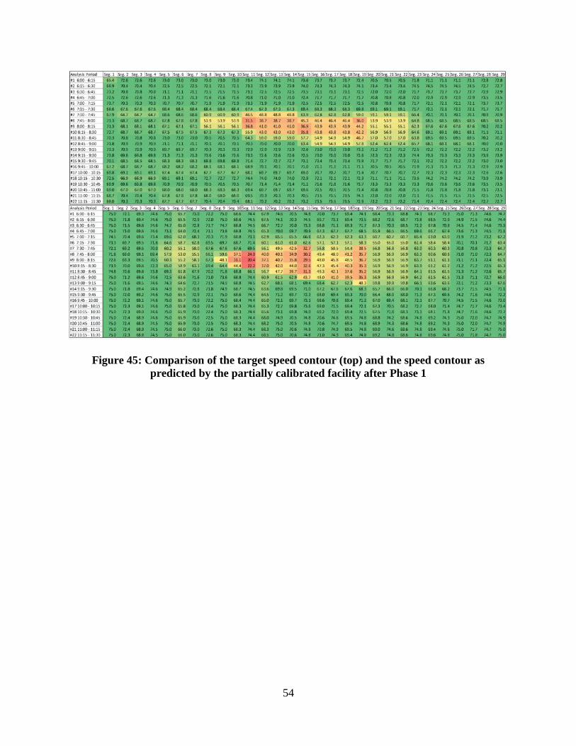
54
Figure 45: Comparison of the target speed contour (top) and the speed contour as
predicted by the partially calibrated facility after Phase 1

55
Table 19: Facility travel times based on the target speeds compared to those from the
facility after Phase 1 calibration

56
4.3.9 Phase 2 Calibration Results
Overall, the Phase 1 calibration showed a large improvement over the initial uncalibrated
model and reduced many of the largest speed errors. Though there was a small increase in the
average facility error, the maximum error for an individual study period was reduced, and the
speed contour reflects the target behavior much more faithfully. However, this only represents a
partial calibration, and two key aspects of capacity calibration have yet to be addressed. This
partially calibrated model can now be run through Phase 2 of the calibration to estimate the set of
pre-breakdown capacity adjustments, as well as the adjust the facility wide jam density. A range
of 0.85 to 1.05 was specified for the set of pre-breakdown CAFs of each HCM segment. A range
of 180 to 220 veh/mi/ln was used for the facility-wide jam density. Based on the size of the facility
and the length of the study period, an initial population size of 200 organisms was specified. Table
20 summarizes the parameters, and five GA runs were conducted to calibrate the facility.
Table 20: Summary of the parameters used for the Phase 2 calibration runs
Running Phase 2 calibration successfully estimated a set of pre-breakdown capacity
adjustments as well as the facility-wide jam density. The set of pre-breakdown CAFs can be seen
in Figure 47, and the capacity drop was estimated to be 5%, while the facility-wide jam density
was estimated to be 189 veh/mi/ln. A summary of the average absolute speed errors for different
speed regimes can be found in Table 21. Additionally, Figure 46 shows a comparison of the target
speed contour and the new partially calibrated speed contour, while Table 22 provides a full
breakdown of the remaining error between the target and predicted travel times, as well as
improvements over the Phase 1 calibration. The Phase 2 calibration show improvement on both
the total speed error, as well as for the individual speed regimes. Perhaps most importantly, a
model calibrated through the two stage process showed a reduction in speed error of over 60% for
speeds lower than 65mph, and a reduction of 70% for all speeds lower than 55 mph! In terms of
travel time, Table 22 shows a further reduction in error for most analysis periods. All but one
analysis period falls within 10% of the target travel time, and the average error is just 2.1%.
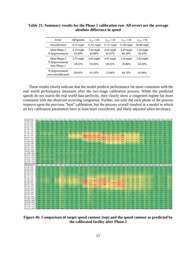
57
Table 21: Summary results for the Phase 1 calibration run. All errors are the average
absolute difference in speed
These results clearly indicate that the model predicts performance far more consistent with the
real world performance measures after the two-stage calibration process. While the predicted
speeds do not match the real world data perfectly, they clearly show a congested regime far more
consistent with the observed recurring congestion. Further, not only did each phase of the process
improve upon the previous “best" calibration, but the process overall resulted in a model in which
all key calibration parameters have at least been considered, and likely adjusted when necessary.
Figure 46: Comparison of target speed contour (top) and the speed contour as predicted by
the calibrated facility after Phase 2

58
Table 22: Facility travel times based on the target speeds compared to those from facility
after Phase 2 calibration

59
Figure 47 shows the set of pre-breakdown CAFs as estimated by the GA algorithm. It is
immediately clear that there exists some “noise" within the generated values, and the capacity of
some segments has been adjusted even when no adjustment was needed. This can occur due a lack
of sensitivity to the parameter for segments whose D/C ratio is significantly below 1.0. In these
cases, neither increasing nor decreasing the capacity has much if any effect on the predicted speeds.
Consequently, it may be prudent for an analyst to perform a basic sensitivity analysis to re-adjust
some of the estimated CAFs back to the default value. Alternatively, the encoding proposed
previously could be adjusted to explicitly constrain the location and/or number of allowed pre-
breakdown adjustments. It will be clear for certain facilities, for geometric or other factors, there
are a specific number of bottlenecks, or bottlenecks at specific locations, that require pre-
breakdown adjustments to be estimated. It is possible to constrain how the set of pre-breakdown
CAFs is determined by altering the existing coding for pre-breakdown CAFs proposed earlier. The
altered encoding should allow both the location and the value of a pre-specified number of CAFs
to be varied by the GA framework. A special case of this encoding can be developed where both
the number and location of the CAFs is specified by an analyst, and only the adjustment value is
varied by the GA search process.
Figure 47: Chart showing the set of pre-breakdown CAFs for all segments of the facility as
estimated during the Phase 2 calibration process
If an analyst specifies that n pre-breakdown CAFs should be determined, the encoding will
have 2n variables, one segment index variable and one adjustment value for each location. The
adjustment can be encoded into a binary string in the same manner as for the full set of adjustments
106 presented previously, but the array of segment locations must be treated as a real-valued array
if it is not fixed by the analyst. Unfortunately, the segment locations cannot be encoded as binary
values because a single integer value that is not a power of two cannot readily be represented as a
binary string. Unlike floating point values, when dealing solely with integers, step sizes and basic
rounding cannot be employed as there is no general way to ensure the representation is balanced
across the full search range. However, when dealing with an array of integer values, the individual
values can maintain their base 10 representation, and the array can be treated in largely the same
manner as a binary string. Most common crossover operators would require no adjustment as they
simply switch values between arrays. Mutation operators will require slight alterations as they
have to consider the range of values for the integer value using a probability distribution (e.g.,

60
uniform or Gaussian) instead of just the two binary possibilities. While real-value GA encodings
such as this are not uncommon, they do lack many of the most desirable properties of a binary
encoding, and may result in slower convergence. In the event that the number adjustments is
limited to just one segment, an exhaustive search is likely a better option than the GA framework.
Further, an exhaustive search is computationally tractable regardless of whether the location of the
single adjustment is fixed or allowed to vary. The computational time should not exceed that of
the GA approach, and the optimal solution is guaranteed to be found. With a CAF step size of
0.001 and a range of [0.5,1.0], there are 500 potential values for the adjustment. If the location of
the adjustment is fixed, the FREEVAL core engine would need to be invoked 500 times, which
would have a computational burden equivalent to evolving a population of 100 organisms for 5
generations. This is less than 1% of the effort spent in each of the calibration phases for this case
study where a population of 200 organisms was evolved over 400 generations. Even if the location
of the adjustment is not fixed, and is allowed to be any of a facility’s segments, the burden still
remains comparatively small. It is highly unlikely a facility will have more than 50 segments, and
if the exhaustive search must be conducted for as many as 50 segments, the computational burden
still remains less than 50% of a typical phase of the calibration process. Further, if the step size is
limited to 0.01, the burden is reduced by a factor of ten! This special case of allowing a single CAF
to be adjusted was explored for the I-540 case study. The exhaustive search approach for the single
pre-breakdown capacity adjustment at an unknown segment location was performed. The search
determined that the optimal location for the CAF is at segment 15, and the optimal CAF value is
0.94. Table 23 shows a breakdown of the remaining errors in speeds by regime for this special case
Phase 2 calibration, and Figure 48 shows the new speed contour. While the reduction in speed
error is not quite as good as when the full set of CAFs is allowed to be adjusted, the special case
Phase 2 still showed significant improvement over the Phase 1 calibration. Further, it provides a
more easily justifiable alteration of capacities for the facility. 107 The adjustment at segment 15
caused the D/C ratio to be above 1.0 for analysis periods 8 and 9 (7:45am-8:15am) leading to the
active bottleneck as seen in both the target and predicted contours.
Table 23: Summary results for the Phase 1 calibration run, all errors are the average
absolute difference in speed

61
Figure 48: Comparison of target speed contour (top) and the speed contour as predicted by
the methodology after the special case Phase 2 calibration with a single CAF
62
5.0 CONCLUSIONS
This project focused on the HCM freeway facilities analysis which plays the core role in other
freeway analysis types. Other facility-based analysis in HCM is built on freeway facilities
methodology such as travel time reliability, Active Traffic and Demand Management (ATDM), or
Work Zone analyses. This research focused on the use of avaible data sources to streamline the
HCM freeway analysis. Examples of availble data sources were investigated are a) online mapping
tools and b) sensor data providing speeds. These data sources can be utilized to aid analysts
perform freeway segmentation as well as demand estimation and calibration.
The research team investigated different online mapping services and evaluated information
that can be gathered through these data sources. Google Maps API selected to be the best data
provider for geometric data needs for freeway analysis. Beside this effort, the project team
developed a segmentation procedure that can divide a freeway strech into HCM segments. The
resulting HCM segments are completely matching with HCM definitions. The project team
implemented the developed segmentation procedure in FREEVAL. Google Maps API also
emplyed to assist analysts fill requried information (e.g. sections lengths) automatically. As a
result, the entire procedure of segmentatin automated in FREEVAL computational engine.
The project also developed methods to estimate demand and calibrate analysis based on
availble sensor data. The most uniform sensor database availble across US is probe-based speed
data. There are several number of probe-based speed data providers such as INRIX, Here.com,
and etc. The developed models to estimate demand and calibrate FREEVAL to target speed
profiles/contours carried out by tuning speed, capacity and demand adjustment factors. The
proposed method implemented in FREEVAL, and can be invoked to perform demand estimation
and analysis calibration.
The calibration approach uses a genetic algorithm metaheuristic to automate the arduous
process of concurrently adjusting large numbers of parameters to ensure the model predicts
performances that matches observed real-world conditions. This project presents two encoding
approaches for traffic demand estimation and adjustment. Each encoding requires an analyst to
have access to average annual daily traffic (AADT) values for each entry and exit node of the
facility, and allows general knowledge of demand patterns to be incorporated when available.
Considering model calibration phase, it was found that demand estimation and adjustment
using the GA framework was shown to significantly improve upon uncalibrated facilities without
any manual adjustments of inputs by the analyst. Combining the approach for demands with key
capacity parameters resulted in an even more effective unified calibration framework. Each phase
of the calibration shows significant improvement over both the uncalibrated facility and the
previous best available calibration. Calibrating for both facility travel time and individual segment
speeds in conjunction yields a more accurate model than calibrating facility travel time only and
can eliminate cases where closely matching target and predicted travel times are misleading. When

63
the capacity of every segment along a facility is allowed to be adjusted, it was found that situations
may arise where conflicting or unrealistic adjustments occur, likely due to overparameterization.
In summary, the automated system identification approach developed in this project represents
a major improvement over the existing best practice for model calibration. The genetic algorithm
framework greatly reduces the burden placed on the user and closes the gap between model
creation and model utilization, a process that represents the biggest challenge for prospective
analysts. Uncalibrated or poorly calibrated models have little to no practical use and consequently
facility calibration is critical for utilizing the HCM methodology effectively.
Finally, the genetic algorithm framework in this research dealt strictly with calibrating a
facility of the core HCM freeway facilities level. However, with slight modification, the scope of
the calibration approach can be greatly expanded. Remaining within the HCM, in the event that
data is available, encodings could be developed and studied for calibration of aspects of reliability
analysis that spans study periods of months or even years.

64
6.0 REFERENCES
Blum, C. & Roli, A. (2003). “Metaheuristics in combinatorial optimization: Overview and
conceptual comparison”. ACM Computing Surveys (CSUR) 35.3, pp. 268–308.
Carey, M. & Watling, D. (2012). “Dynamic traffic assignment approximating the kinematic
wave model: System optimum, marginal costs, externalities and tolls”. Transportation Research
Part B: Methodological 46.5, pp. 634–648.
Carey, M. et al. (2014a). “Extending travel-time based models for dynamic network loading and
assignment, to achieve adherence to first-in-first-out and link capacities”. Transportation
Research Part B: Methodological 65, pp. 90–104.
Carey, M. et al. (2014b). “Implementing first-in–first-out in the cell transmission model for
networks”. Transportation Research Part B: Methodological 65, pp. 105–118.
Chiu, Y.-C. et al. (2011). “Dynamic traffic assignment: A primer”. Transportation Research E-
Circular E-C153.
Coello, C. A. C. (2002). “Theoretical and numerical constraint-handling techniques used with
evolutionary algorithms: a survey of the state of the art”. Computer Methods in Applied
Mechanics and Engineering 191.11, pp. 1245–1287.
Daganzo, C. F. (1994). “The cell transmission model: A dynamic representation of highway
traffic consistent with the hydrodynamic theory”. Transportation Research Part B:
Methodological 28.4, pp. 269 –287.
— (1995). “The cell transmission model, part 2: Network traffic”. Transportation Research Part
B: Methodological 29.2, pp. 79 –93.
De Nicolao, G (1997). “System identification: Problems and perspectives”. 12th Workshop on
Qualitative Reasoning, pp. 379–386.
Delbem, A. C. et al. (2012). “Efficient forest data structure for evolutionary algorithms applied
to network design”. Evolutionary Computation, IEEE Transactions on 16.6, pp. 829–846.
Doan, K. & Ukkusuri, S. V. (2012). “On the holding-back problem in the cell transmission based
dynamic traffic assignment models”. Transportation Research Part B: Methodological 46.9, pp.
1218 –1238.
Elefteriadou, L. & Lertworawanich, P. (2003). “Defining, measuring and estimating freeway
capacity”. Washington: Transportation Research Board Meeting.
Gendreau, M. & Potvin, J.-Y. (2005). “Metaheuristics in combinatorial optimization”. Annals of
Operations Research 140.1, pp. 189–213. 117

65
Goldberg, D. E. (1989). Genetic Algorithms in Search, Optimization and Machine Learning. 1st.
Boston, MA, USA: Addison-Wesley Longman Publishing Co., Inc.
Gomes, G. & Horowitz, R. (2006). “Optimal freeway ramp metering using the asymmetric cell
transmission model”. Transportation Research Part C: Emerging Technologies 14.4, pp. 244 –
262.
Gomes, G. et al. (2008). “Behavior of the cell transmission model and effectiveness of ramp
metering”. Transportation Research Part C: Emerging Technologies 16.4, pp. 485 –513.
Hadi, M. et al. (2014). “Pilot Testing of SHRP 2 Reliability Data and Analytical Products:
Florida Pilot Site”. SHRP 2 Report.
Hallenbeck, M. et al. (1997). Vehicle volume distributions by classification. Tech. rep.
Han, L. et al. (2011). “Complementarity formulations for the cell transmission model based
dynamic user equilibrium with departure time choice, elastic demand and user heterogeneity”.
Transportation Research Part B: Methodological 45.10, pp. 1749 –1767.
Highway CapacityManual(2016). 6th Edition: A Guide forMultimodalMobility Analysis.
Washington, D.C.: Transportation Research Board.
Hu, J. et al. (2012). “On linear programs with linear complementarity constraints”. English.
Journal of Global Optimization 53.1, pp. 29–51.
Juan, W. et al. (2012). “Genetic algorithm for multiuser discrete network design problem under
demand uncertainty”. Mathematical Problems in Engineering 2012.
Karoonsoontawong, A. & Waller, S. (2006). “Dynamic Continuous Network Design Problem:
Linear Bilevel Programming and Metaheuristic Approaches”. Transportation Research Record:
Journal of the Transportation Research Board 1964, pp. 104–117. eprint: http://dx.doi.org/10.
3141/1964-12.
Li, Y. et al. (2003). “A Decomposition Scheme for System Optimal Dynamic Traffic
Assignment Models”. Networks and Spatial Economics 3.4.
Li, Z.-b. et al. (2014). “Development of control strategy of variable speed limits for improving
traffic operations at freeway bottlenecks”. English. Journal of Central South University 21.6, pp.
2526– 2538.
Lighthill, M. J. & Whitham, G. B. (1955a). “On Kinematic Waves. I. Flood Movement in Long
Rivers”. English. Proceedings of the Royal Society of London. Series A, Mathematical and
Physical Sciences 229.1178, pp. 281–316.
Lighthill, M. J. & Whitham, G. B. (1955b). “On Kinematic Waves. II. A Theory of Traffic Flow
on Long Crowded Roads”. Proceedings of the Royal Society of London A: Mathematical,
Physical and Engineering Sciences 229.1178, pp. 317–345.

66
Lim, G. J. et al. (2015). “Reliability analysis of evacuation routes under capacity uncertainty of
road links”. IIE Transactions 47.1, pp. 50–63. eprint: http://dx.doi.org/10.1080/0740817X.
2014.905736.
Lin, D.-Y. et al. (2011). “A Dual Variable Approximation Based Heuristic for Dynamic
Congestion Pricing”. English. Networks and Spatial Economics 11.2, pp. 271–293.
Lin, W.-H. & Ahanotu, D. (1995). “Validating the basic cell transmission model on a single
freeway link”. PATH technical note; 95-3.
Ljung, L. (2010). “Perspectives on system identification”. Annual Reviews in Control 34.1, pp.
1–12.
Lo, H. K. (2001). “A Cell-Based Traffic Control Formulation: Strategies and Benefits of
Dynamic Timing Plans”. English. Transportation Science 35.2, pp. 148–164.
Lu, C.-C. et al. (2013). “Dynamic origin–destination demand flow estimation under congested
traffic conditions”. Transportation Research Part C: Emerging Technologies 34, pp. 16–37.
Luathep, P. et al. (2011). “Global optimization method for mixed transportation network design
problem: A mixed-integer linear programming approach”. Transportation Research Part B:
Methodological 45.5, pp. 808 –827.
Ma, T. et al. (2015). “Nonlinear multivariate time space threshold vector error correction model
for short term traffic state prediction”. Transportation Research Part B: Methodological 76.0, pp.
27 –47.
Malveo, A. E. (2013). Assessing the Impact of Congestion During a Multi-County Evacuation.
Tech. rep. DTIC Document.
Maryland CATT Lab, U. of (2008). RITIS:Regional Integrated Transportation Information
System. URL: https://www.ritis.org/ (visited on 08/11/2016).
Mitchell, M. (1998). An introduction to genetic algorithms. MIT press.
Morbidi, F. et al. (2014). “A new robust approach for highway traffic density estimation”.
Control Conference (ECC), 2014 European, pp. 2575–2580.
Mudchanatongsuk, S. et al. (2008). “Robust Solutions for Network Design under Transportation
Cost and Demand Uncertainty”. English. The Journal of the Operational Research Society 59.5,
pp. 652–662. 119
Munoz, L. et al. (2003). “Traffic density estimation with the cell transmission model”. American
Control Conference, 2003. Proceedings of the 2003. Vol. 5, 3750–3755 vol.5.
Muñoz, L. et al. (2004). “Methodological calibration of the cell transmission model”. American
Control Conference, 2004. Proceedings of the 2004. Vol. 1. IEEE, pp. 798–803.

67
NCDOT (2016). Planning Level Extensions to NCDOT Freeway Analysis Tools. URL: https://
connect.ncdot.gov/projects/planning/Pages/ProjDetails.aspx?ProjectID= 2015-09.
Nisbet, J. et al. (2014). Pilot Testing of SHRP 2 Reliability Data and Analytical Products:
Washington.
North Carolina Department of Transportation (2016). Traffic Surveys. URL: https://www.ncdot.
gov/projects/trafficsurvey/ (visited on 08/11/2016).
Pascale, A. et al. (2013). “Estimation of highway traffic from sparse sensors: Stochastic
modeling and particle filtering”. Acoustics, Speech and Signal Processing (ICASSP), 2013 IEEE
International Conference on, pp. 6158–6162.
Pascale, A. et al. (2014). “Cooperative Bayesian Estimation of Vehicular Traffic in Large-Scale
Networks”. Intelligent Transportation Systems, IEEE Transactions on 15.5, pp. 2074–2088.
Richards, P. I. (1956). “Shock Waves on the Highway”. English. Operations Research 4.1, pp.
42–51.
Smilowitz, K. & Daganzo, C. (1999). “Predictability of time-dependent traffic backups and other
reproducible traits in experimental highway data”. California Partners for Advanced Transit and
Highways (PATH).
Sobolewski, M. et al. (2014). Pilot Testing of SHRP 2 Reliability Data and Analytical Products:
Minnesota.
Stankova, K. & De Schutter, B. (2010). “On freeway traffic density estimation for a jump
Markov linear model based on Daganzo’s cell transmission model”. Intelligent Transportation
Systems (ITSC), 2010 13th International IEEE Conference on, pp. 13–18.
Sumalee, A. et al. (2011). “Stochastic cell transmission model (SCTM): A stochastic dynamic
traffic model for traffic state surveillance and assignment”. Transportation Research Part B:
Methodological 45.3, pp. 507 –533.
Sun, H. et al. (2014). “Dynamic Network Design Problem under Demand Uncertainty: An
Adjustable Robust Optimization Approach”. Discrete Dynamics in Nature and Society 2014.
Tampère, C. & Immers, L. (2007). “An Extended Kalman Filter Application for Traffic State
Estimation Using CTM with Implicit Mode Switching and Dynamic Parameters”. Intelligent
Transportation Systems Conference, 2007. ITSC 2007. IEEE, pp. 209–216.
Travis Waller, S. & Ziliaskopoulos, A. K. (2006). “A Combinatorial user optimal dynamic traffic
assignment algorithm”. English. Annals of Operations Research 144.1. Copyright - Springer
Science+Business Media, LLC 2006; Last updated - 2014-08-30, pp. 249–261.
Ukkusuri, S. V. & Waller, S. T. (2008). “Linear Programming Models for the User and System
Optimal Dynamic Network Design Problem: Formulations, Comparisons and Extensions”.
English. Networks and Spatial Economics 8.4, pp. 383–406.

68
Ukkusuri, S. V. et al. (2012). “Dynamic user equilibrium with a path based cell transmission
model for general traffic networks”. Transportation Research Part B: Methodological 46.10, pp.
1657 –1684.
Waller, S. & Ziliaskopoulos, A. (2001). “Stochastic Dynamic Network Design Problem”.
Transportation Research Record: Journal of the Transportation Research Board 1771, pp. 106–
113. eprint: http: //dx.doi.org/10.3141/1771-14.
Williges, C. et al. (2014). Pilot Testing of SHRP 2 Reliability Data and Analytical Products:
Southern California Pilot Site. Tech. rep.
Xu, T. et al. (2009). “Study on continuous network design problem using simulated annealing
and genetic algorithm”. Expert Systems with Applications 36.2, Part 2, pp. 2735 –2741.
Yao, T. et al. (2009). “Evacuation Transportation Planning Under Uncertainty: A Robust
Optimization Approach”. English. Networks and Spatial Economics 9.2, pp. 171–189.
Zeng, Q. & Mouskos, K. C. (1997). “Heuristic search strategies to solve transportation network
design problems”. Final report to the New Jersey Department of Transportation and the National
Center for Transportation and Industrial Productivity.
Zheng, H. & Chiu, Y.-C. (2011). “A Network Flow Algorithm for the Cell-Based Single-
Destination System Optimal Dynamic Traffic Assignment Problem”. Transportation Science
45.1, pp. 121– 137. eprint: http://dx.doi.org/10.1287/trsc.1100.0343.
Zhong, R. et al. (2013). “A linear complementarity system approach to macroscopic freeway
traffic modeling”. Cyber Technology in Automation, Control and Intelligent Systems (CYBER),
2013 IEEE 3rd Annual International Conference on, pp. 18–23.
Zhong, R. et al. (2014). “Towards automatic model calibration of first-order traffic flow model”.
Control Conference (CCC), 2014 33rd Chinese, pp. 3423–3428.
Zhu, F. & Ukkusuri, S. V. (2013). “A cell based dynamic system optimum model with non-
holding back flows”. Transportation Research Part C: Emerging Technologies 36, pp. 367 –380.
Ziliaskopoulos, A. K. (2000). “A Linear Programming Model for the Single Destination System
Optimum Dynamic Traffic Assignment Problem”. English. Transportation Science 34.1, pp. 37–
49.