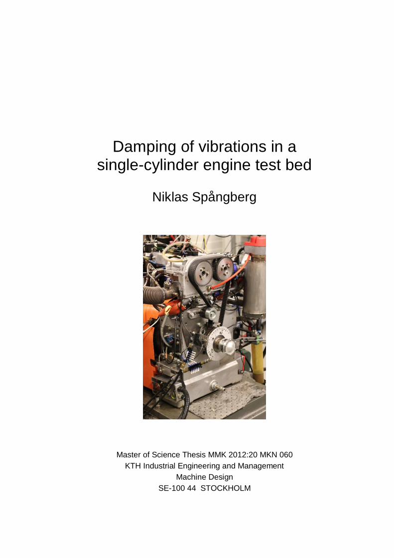
Damping of vibrations in a single-cylinder engine test bed

NIKLAS SPÅNGBERG

Master of Science Thesis

Stockholm, Sweden 2012

Damping of vibrations in a single-cylinder engine test bed

Niklas Spångberg

Master of Science Thesis MMK 2012:20 MKN 060

KTH Industrial Engineering and Management

Machine Design

SE-100 44 STOCKHOLM

i

Master of Science Thesis MMK 2012:20 MKN 060

Damping of vibrations in a

single-cylinder engine test bed

Niklas Spångberg

Approved

2012-06-05

Examiner

Ulf Sellgren

Supervisor

Ulf Sellgren, KTH

Björn Zachrisson,AVL MTC

Commissioner

AVL MTC

Contact person

Erik Karlsson

Abstract

A study has been conducted to analyze the vibration behavior of one of AVLs light-duty engine

test beds, used to develop and test new combustion engine concepts.

It has previously been observed that the test bed exerts large vibrations as the engine speed

approaches 3000 rpm. As the test bed is mainly used for testing spark-ignited combustion engine

concepts, it is desired to conduct measurements at engine speeds up to 6000 rpm. Therefore the

purpose of the study is to find a new design for the test bed which reduces the speed-related

vibrations and allow the engine to run at speeds up to 6000 rpm. In addition, the study has sought

to find an appropriate method of measuring the engine torque in a more precise way than

previous measurement methods.

The test bed components such as the engine, driveshaft, flywheel, couplings and the electric

motor have been analyzed to determine the influence the mentioned components have on the

vibration modes of the test bed. A theoretical model of the test bed components as a system was

built in MATLAB, the model was then used to find the optimal dimensions of each component

in order to reduce the vibrations. The accuracy of the model was verified using measured engine

data; In addition, the vibration modes of the test bed were measured using an accelerometer

mounted on the electric motor. The measured data was processed using PULSE. A CAD model

of a new test bed concept was created using Autodesk Inventor. The vibration modes of the new

test bed were verified using ANSYS.

The study concludes that the components generally need to have a higher stiffness as well as a

lower moment of inertia in order to reduce the risk of critical resonances being generated at

speeds below 6000 rpm. In particular, the inertia of the engine flywheel and the couplings for the

driveshaft should be reduced by 50% and 57 % respectively. Furthermore, the counterweight

mass of the engine crankshaft should be reduced to 1.32 kg for the balance degree of the engine

to lower than 36%, in order to reduce lateral inertial forces in the engine. However, the study

concludes that lowering the inertia of these components will cause the fluctuations in speed to

increase from the current average value of 2 rpm to 4 rpm.

Finally, the study concludes that a digital torque sensor should be used to achieve the desired

measurement accuracy.

ii

iii

Examensarbete MMK 2012:20 MKN 060

Dämpning av vibrationer i en

encylindrig motorprovcell

Niklas Spångberg

Godkänt

2012-06-05

Examinator

Ulf Sellgren

Handledare

Ulf Sellgren, KTH

Björn Zachrisson, AVL MTC

Uppdragsgivare

AVL MTC

Kontaktperson

Erik Karlsson

Sammanfattning En studie har genomförts för att analysera vibrationsbeteendet hos en av AVLs encylindriga

motorprovceller som används för att utveckla och testa nya förbränningsmotorkoncept.

Det har tidigare konstaterats att stora vibrationer uppstå i provcellen då motorvarvtalet närmar

sig 3000 varv/min. Eftersom provcellen främst används att testa bensinmotorkoncept är det

önskvärt att kunna utföra mätningar vid motorvarvtal upp till 6000 varv/minut. Syftet med

studien är därför att analysera och utveckla ett koncept för en konstruktionsförändring av riggen

som minskar de hastighetsrelaterade vibrationerna och tillåter att motorn körs i hastigheter upp

till 6000 rpm. Förutom detta så har studien syftat till att hitta en lämplig metod för att mäta

motorns vridmoment på ett mer precist sätt än tidigare.

Provcellens komponenter såsom motor, drivaxel, svänghjul, kopplingar och elmotorn har

analyserats för att avgöra hur komponenterna påverkar vibrationer i provcellen.

En teoretisk modell av provcellskomponenterna som ett system upprättades i MATLAB,

modellen användes sedan för att hitta de optimala dimensionerna för varje komponent för att

minska vibrationerna. Noggrannheten av modellen verifierades med uppmätt motordata.

Vibrationerna i provcellen mättes dessutom med en accelerometer som fästes på elmotorn,

mätdatan från provningarna bearbetades sedan med PULSE. En CAD-modell av det nya

provcellskonceptet skapats med Autodesk Inventor, och vibrationsmoderna verifierades i

ANSYS.

I studien dras slutsatsen att provcellens komponenter i allmänhet behöver ha en högre styvhet

samt ett lägre tröghetsmoment för att motverka att kritiska resonanser uppkommer före 6000

varv/minut. I synnerhet bör tröghetsmomenten för motorns svänghjul och drivaxelns kopplingar

minskas med 50% respektive 57%. Vidare bör motviktsmassan för motorns vevaxel reduceras

1.32 kg för att motorns balansgrad skall understiga 36 %, i syfte att minska horisontella

svängningar i motorn som orsakas av tröghetskrafter. Dock konstateras även att om trögheten

sänks för dessa komponenter, medför det att variationerna för rotationshastigheten ökar från i

snitt 2 varv/minut till i snitt 4 varv/minut

Slutligen fastställer studien att en digital vridmomentsensor bör användas för att uppnå den

önskade mätnoggrannheten.

iv

v

ACKNOWLEDGEMENTS

I would like to extend my thanks to the following people at AVL for your invaluable help during

the period of my thesis:

Björn Zachrisson for supervising the thesis work.

Johannes Andersén for providing additional supervision and support.

Gustav Ericsson for all the time spent in the test bed and for getting the engine up-and-running.

Fredrik Königsson for lending me the knock-module for the test bed control system.

Joakim Karlsson for assisting in operating the test bed control system.

Christer Thelin for all the help and guidance during the vibration measurements.

Carl-Henrik Ericson, Petri Fransman and Anders Knutsson for the additional help in the test bed.

Richard Backman, Erik Karlsson and Johan Wohlfart for accepting me to start the thesis to begin

with, and for the input during the initial phase of the work.

Last but not least: my supervisor at KTH, Ulf Sellgren, for the supervision and support.

Niklas Spångberg

Stockholm, June 2012

vi

vii

NOMENCLATURE

This section describes the denotations and abbreviations used in the thesis.

Denotations

Symbol Description

a Acceleration (m/s2)

A Area (m2)

c Torsion stiffness (Nm/rad)

d Diameter (m2)

D Bending stiffness (Nm)

E Young’s modulus (Pa)

G Shear modulus (Pa)

F Force (N)

H Power (W)

J Moment of inertia (kgm2)

k Spin effect (rad/m)

K Polar moment of inertia of area (m4)

l Connecting rod length (m)

L Driveshaft length (m)

m mass (kg)

n Speed (rev/min)

p pressure (bar)

P Vibration constant (-)

q Pulse ratio (-)

r Radius (m)

t Time (s)

T Torque (Nm)

v Velocity (m/s)

V Volume (m3)

W Work (Nm)

x Position (m)

X Displacement (m)

viii

y Spin-inertia (m-2

)

z Transverse inertia (m-4

)

Equivalent inertia (m-1

)

Equivalent inertia (m-1

)

Transverse frequency (rad/s)

ε Compression ratio (-)

ζ Balance degree (-)

Rod angle (°)

Specific heat ratio (-)

Shaft/rod ratio (-)

Poisson’s ratio (-)

Density (kg/m3)

Crank angle degree (°)

Degree of speed fluctuation (-)

Ψ Degree of work fluctuation (-)

Angular velocity (rad/s)

Abbreviations

BDC Bottom Dead Center

BSFC Brake Specific Fuel Consumption

CAD Computer Aided Design

FEM Finite Element Method

TDC Top Dead Center

ix

TABLE OF CONTENTS

1 INTRODUCTION 1

1.1 Background 1

1.2 Problem description 1

1.3 Aims 2

1.4 Delimitations 2

1.5 Methodology 2

2 FRAME OF REFERENCE 3

2.1 Test bed overview 3

2.2 Combustion engines 10

2.3 Couplings 11

2.4 Flywheels 14

2.5 Driveshafts 15

2.6 Torque sensors 16

3 ANALYSIS & DIMENSIONING 19

3.1 Engine torque dynamics 19

3.2 Inertia and stiffness of components 29

3.3 Resonance frequencies and critical speeds 32

3.4 Dimensioning the flywheel 35

3.5 Dimensioning the drive shaft 43

3.6 Dimensioning the couplings 43

3.7 Dimensioning the crankshaft 45

3.8 Dimensioning the torque sensor 47

4 RESULTS 49

4.1 Overview 49

4.2 Crankshaft 50

4.3 Flywheel 50

4.4 Driveshaft 51

4.5 Couplings 51

x

4.6 Torque sensor 52

5 VERIFICATION 55

6 DISCUSSION AND CONCLUSIONS 57

6.1 Discussion 57

6.2 Conclusions 57

7 RECOMMENDATIONS AND FUTURE WORK 59

7.1 Recommendations 59

7.2 Future work 59

8 REFERENCES 61

APPENDIX A: Test bed specifications 63

APPENDIX B: Bessel functions 65

1

1 INTRODUCTION

This chapter describes the background, problem description, aims, delimitations, and methods

used in the thesis work.

1.1 Background

AVL uses a spark-ignited, single-cylinder engine test bed to perform research on new engine

concepts such as free valve timing and the use of alternative fuels. The test bed is designed to

measure important engine performance parameters such as torque, speed, power and efficiency

as well as specific fuel consumption and emission levels.

As of today, the engine can only run at a maximum speed of 3000 rpm due to high vibration

levels. These vibrations are believed to be caused by the flywheel mounted on the driveshaft

between the engine and the test bed dynamometer. The difficulty is to maintain a relatively large

moment of inertia to ensure minimal deviations in crank angle speed versus the oscillating loads

that crankshaft and main bearing are exposed to. As a means to minimize the oscillations, AVL

intends to replace to existing drive shaft with a torsion stiff coupling mounted on a cardan shaft.

Another major concern with the test bed is the fact that the total accuracy level of the instruments

and sensors measuring the output torque of the engine has not yet been fully determined. A more

precise method for measuring the torque should lead to better accuracy when measuring engine

power, specific fuel consumption among others.

1.2 Problem description

The thesis is divided into subsections based on the different problems that are sought to be

solved.

1.2.1 Damping of vibrations at high speed

How should the new drive driveshaft be designed and dimensioned in order to minimize the

engines vibration at high speeds? How should the flywheel position and inertia be dimensioned

to eliminate the vibration?

1.2.2 Engine balance

How should the crankshaft be designed to eliminate lateral forces?

1.2.3 Measurement accuracy

How can a torque sensor be installed to increase the accuracy of the torque measurements?

2

1.3 Aims

The primary aims of the thesis are to raise the speed limit of the test bed to 6000 rpm, increase

the accuracy of the torque measurement, and to determine the ideal position, mass, and energy

storage capacity of the flywheel.

The secondary aim is to recommend a more ideal balancing degree of the crankshaft

counterweight in order to minimize the free inertial forces in the vertical direction.

1.4 Delimitations

The work presented in the thesis is limited to study the effects of damping the vibrations in the

test bed by means of using a stiff driveshaft and the influence the flywheel has on the overall

vibrations. The damping will be entirely mechanical, in other words no actively controlled

damping is studied. The study is limited to the analysis of the torsion vibrations in the engine test

bed resonances created due to the rotational motions and torques of the components, therefore no

investigation of the bending critical speeds is perform.

The components studied are limited to the main components of the test bed, i.e. the engine,

driveshaft, and the electric motor – and the components that are part of these subsystems.

The improvement of the measurement accuracy will be based on the implementation of a torque

sensor.

1.5 Methods

The methods for solving the problems presented in the thesis will be based on experiments,

calculations, and simulations. A series of tests will be performed in the test bed in order to

determine the resonance frequencies of the test bed components at critical speeds, as well as

measure the cylinder pressure and inertial force among others. An analytical model based on

theory vibration will be developed based on the results of the test bed measurement. This model

will then be used to find the optimal solutions for drive shaft design and flywheel properties to

minimize the vibrations at high speeds. These results will be verified by solving the model using

FEM.

In order to find the optimal balance degree for the crankshaft of the engine, the inertial forces

from the engine will be measured. The results from the measurements will then be implemented

into an analytical model find the most suitable balance degree. The results will be verified using

FEM.

To improve the accuracy of the torque measurements, a torque sensor will be chosen based on

torque limit and the accuracy after manufacture.

3

2 FRAME OF REFERENCE

This section describes the information that was processed during the thesis literature study. This

information forms the basis for further design and analysis work.

2.1 Test bed overview

Engine test beds are used to test engine parameters that are difficult or impossible to correctly

measure in an in-vehicle environment.

Typical test parameters include fuel efficiency, torque-speed performance; component durability;

aging of oil and lubrications; and exhaust emissions.

An engine test bed typically consists of three major subsystems:

A combustion engine.

An electric motor used during start-up acceleration and braking deceleration of the

engine.

A driveshaft which connects the engine to the electric motor.

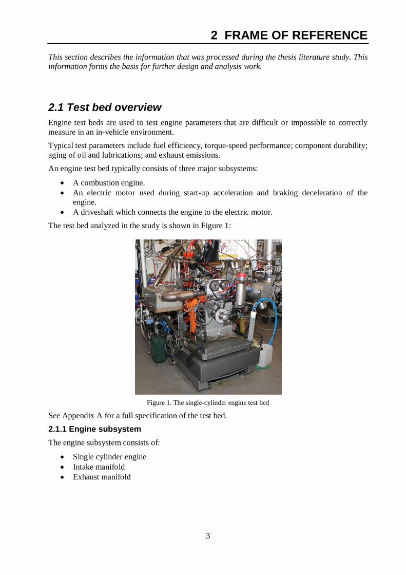
The test bed analyzed in the study is shown in Figure 1:

Figure 1. The single-cylinder engine test bed

See Appendix A for a full specification of the test bed.

2.1.1 Engine subsystem

The engine subsystem consists of:

Single cylinder engine

Intake manifold

Exhaust manifold

4

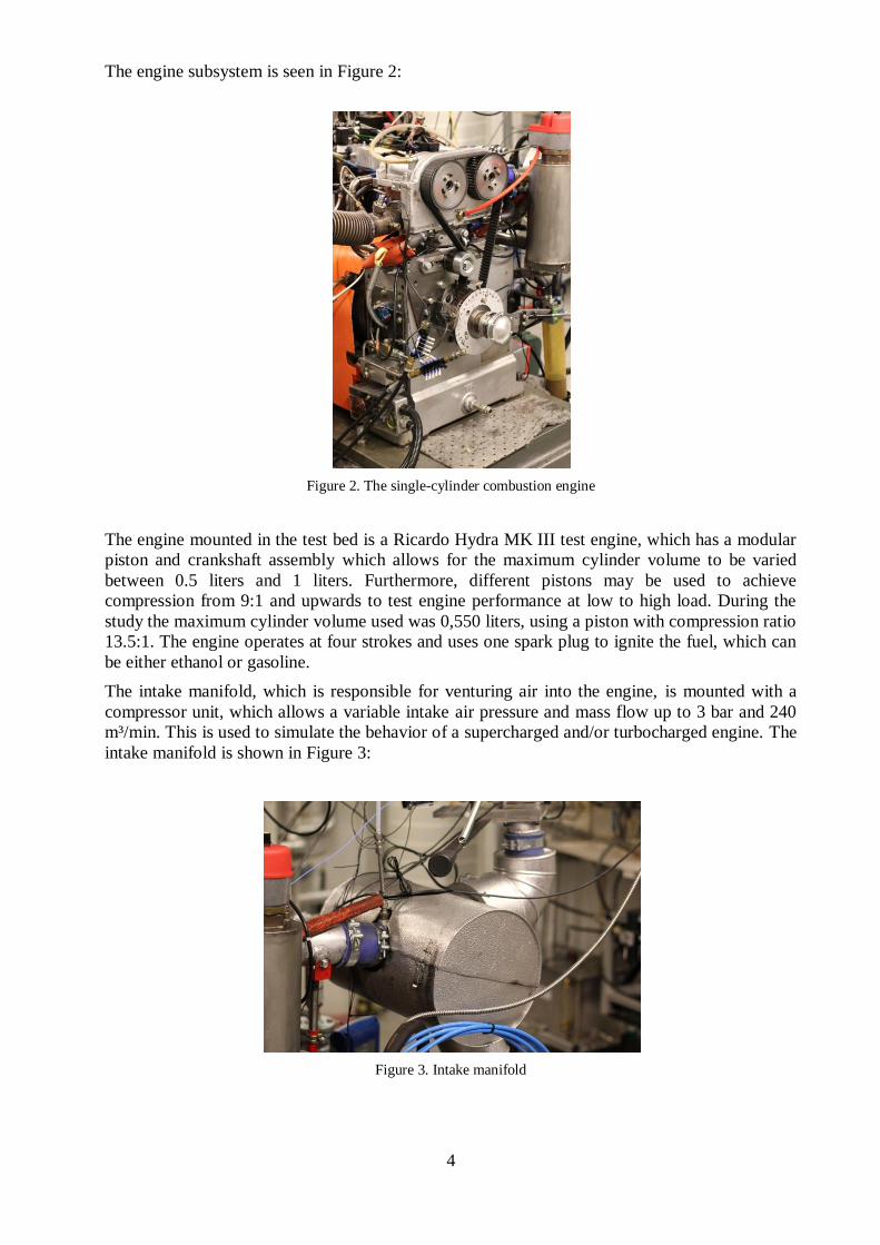
The engine subsystem is seen in Figure 2:

Figure 2. The single-cylinder combustion engine

The engine mounted in the test bed is a Ricardo Hydra MK III test engine, which has a modular

piston and crankshaft assembly which allows for the maximum cylinder volume to be varied

between 0.5 liters and 1 liters. Furthermore, different pistons may be used to achieve

compression from 9:1 and upwards to test engine performance at low to high load. During the

study the maximum cylinder volume used was 0,550 liters, using a piston with compression ratio

13.5:1. The engine operates at four strokes and uses one spark plug to ignite the fuel, which can

be either ethanol or gasoline.

The intake manifold, which is responsible for venturing air into the engine, is mounted with a

compressor unit, which allows a variable intake air pressure and mass flow up to 3 bar and 240

m³/min. This is used to simulate the behavior of a supercharged and/or turbocharged engine. The

intake manifold is shown in Figure 3:

Figure 3. Intake manifold

5

The exhaust manifold releases the hot exhaust gases from the combustion engine at the end of

the combustion. The exhaust manifold of the engine is mounted together with a muffler box,

used to minimize the pressure pulses during the exhaust stroke. The exhaust manifold is shown

in Figure 4:

Figure 4. Exhaust manifold

2.1.2 Driveshaft subsystem

The driveshaft is used for transferring the torque and rotational motion between the engine and

the electric motor.

The driveshaft subsystem consists of:

Shaft

Couplings

Flywheel

A model of the driveshaft subsystem is seen in Figure 5:

Figure 5. Model of the driveshaft subsystem

6

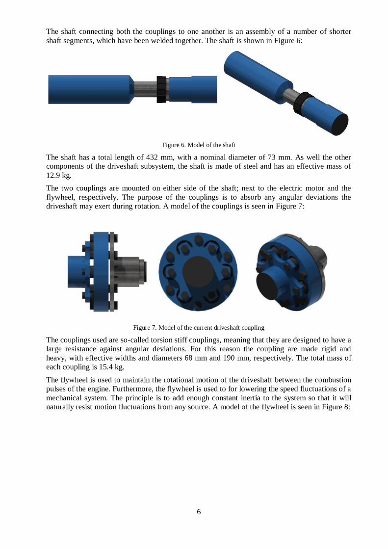
The shaft connecting both the couplings to one another is an assembly of a number of shorter

shaft segments, which have been welded together. The shaft is shown in Figure 6:

Figure 6. Model of the shaft

The shaft has a total length of 432 mm, with a nominal diameter of 73 mm. As well the other

components of the driveshaft subsystem, the shaft is made of steel and has an effective mass of

12.9 kg.

The two couplings are mounted on either side of the shaft; next to the electric motor and the

flywheel, respectively. The purpose of the couplings is to absorb any angular deviations the

driveshaft may exert during rotation. A model of the couplings is seen in Figure 7:

Figure 7. Model of the current driveshaft coupling

The couplings used are so-called torsion stiff couplings, meaning that they are designed to have a

large resistance against angular deviations. For this reason the coupling are made rigid and

heavy, with effective widths and diameters 68 mm and 190 mm, respectively. The total mass of

each coupling is 15.4 kg.

The flywheel is used to maintain the rotational motion of the driveshaft between the combustion

pulses of the engine. Furthermore, the flywheel is used to for lowering the speed fluctuations of a

mechanical system. The principle is to add enough constant inertia to the system so that it will

naturally resist motion fluctuations from any source. A model of the flywheel is seen in Figure 8:

7

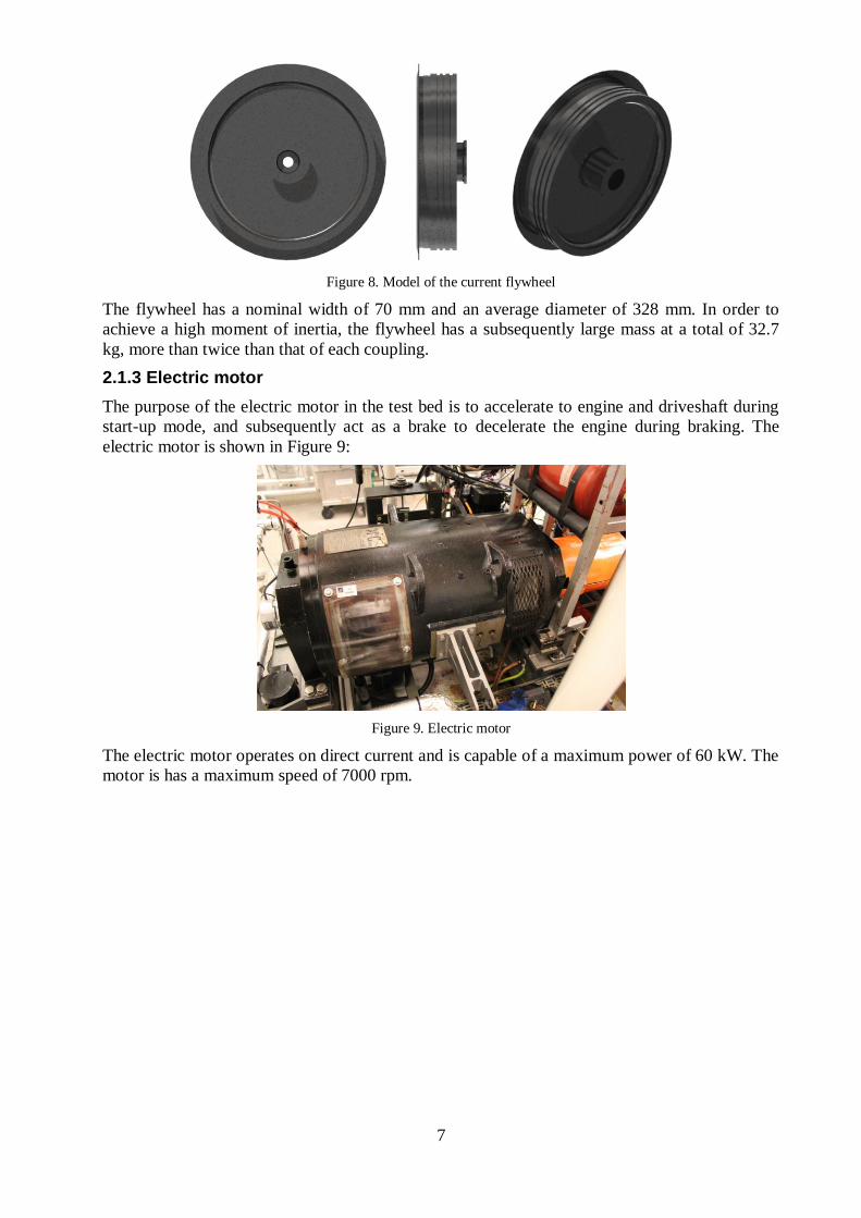
Figure 8. Model of the current flywheel

The flywheel has a nominal width of 70 mm and an average diameter of 328 mm. In order to

achieve a high moment of inertia, the flywheel has a subsequently large mass at a total of 32.7

kg, more than twice than that of each coupling.

2.1.3 Electric motor

The purpose of the electric motor in the test bed is to accelerate to engine and driveshaft during

start-up mode, and subsequently act as a brake to decelerate the engine during braking. The

electric motor is shown in Figure 9:

Figure 9. Electric motor

The electric motor operates on direct current and is capable of a maximum power of 60 kW. The

motor is has a maximum speed of 7000 rpm.

8

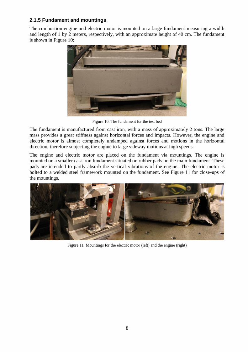
2.1.5 Fundament and mountings

The combustion engine and electric motor is mounted on a large fundament measuring a width

and length of 1 by 2 meters, respectively, with an approximate height of 40 cm. The fundament

is shown in Figure 10:

Figure 10. The fundament for the test bed

The fundament is manufactured from cast iron, with a mass of approximately 2 tons. The large

mass provides a great stiffness against horizontal forces and impacts. However, the engine and

electric motor is almost completely undamped against forces and motions in the horizontal

direction, therefore subjecting the engine to large sideway motions at high speeds.

The engine and electric motor are placed on the fundament via mountings. The engine is

mounted on a smaller cast iron fundament situated on rubber pads on the main fundament. These

pads are intended to partly absorb the vertical vibrations of the engine. The electric motor is

bolted to a welded steel framework mounted on the fundament. See Figure 11 for close-ups of

the mountings.

Figure 11. Mountings for the electric motor (left) and the engine (right)

9

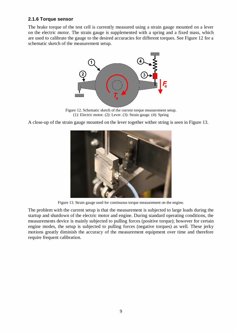
2.1.6 Torque sensor

The brake torque of the test cell is currently measured using a strain gauge mounted on a lever

on the electric motor. The strain gauge is supplemented with a spring and a fixed mass, which

are used to calibrate the gauge to the desired accuracies for different torques. See Figure 12 for a

schematic sketch of the measurement setup.

Figure 12. Schematic sketch of the current torque measurement setup.

(1): Electric motor. (2): Lever. (3): Strain gauge. (4): Spring

A close-up of the strain gauge mounted on the lever together wither string is seen in Figure 13.

Figure 13. Strain gauge used for continuous torque measurement on the engine.

The problem with the current setup is that the measurement is subjected to large loads during the

startup and shutdown of the electric motor and engine. During standard operating conditions, the

measurements device is mainly subjected to pulling forces (positive torque); however for certain

engine modes, the setup is subjected to pulling forces (negative torques) as well. These jerky

motions greatly diminish the accuracy of the measurement equipment over time and therefore

require frequent calibration.

10

2.2 Combustion engines

An internal combustion engine is a power unit used to transform chemical energy into useful

mechanical through the combustion of fuel and air within a combustion chamber. The expansion

of the high-temperature and high-pressure gases produced by the combustion apply a force on a

piston, which is moved downwards in the cylindrical piston chamber. The piston is connected

via a rod to a rotating crankshaft, thereby converting the oscillating motion produced by the gas

force into a rotational output torque.

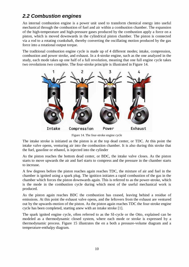
The traditional combustion engine cycle is made up of 4 different modes; intake, compression,

combustion and power stroke, and exhaust. In a 4-stroke engine, such as the one analyzed in the

study, each mode takes up one half of a full revolution, meaning that one full engine cycle takes

two revolutions two complete. The four-stroke principle is illustrated in Figure 14.

Figure 14. The four-stroke engine cycle

The intake stroke is initiated as the piston is at the top dead center, or TDC. At this point the

intake valve opens, venturing air into the combustion chamber. It is also during this stroke that

the fuel, gasoline or ethanol, is injected into the cylinder

As the piston reaches the bottom dead center, or BDC, the intake valve closes. As the piston

starts to move upwards the air and fuel starts to compress and the pressure in the chamber starts

to increase.

A few degrees before the piston reaches again reaches TDC, the mixture of air and fuel in the

chamber is ignited using a spark plug. The ignition initiates a rapid combustion of the gas in the

chamber which forces the piston downwards again. This is referred to as the power-stroke, which

is the mode in the combustion cycle during which most of the useful mechanical work is

produced.

As the piston again reaches BDC the combustion has ceased, leaving behind a residue of

emissions. At this point the exhaust valve opens, and the leftovers from the exhaust are ventured

out by the upwards-motion of the piston. As the piston again reaches TDC the four-stroke engine

cycle has been completed, starting anew with an intake stroke [1].

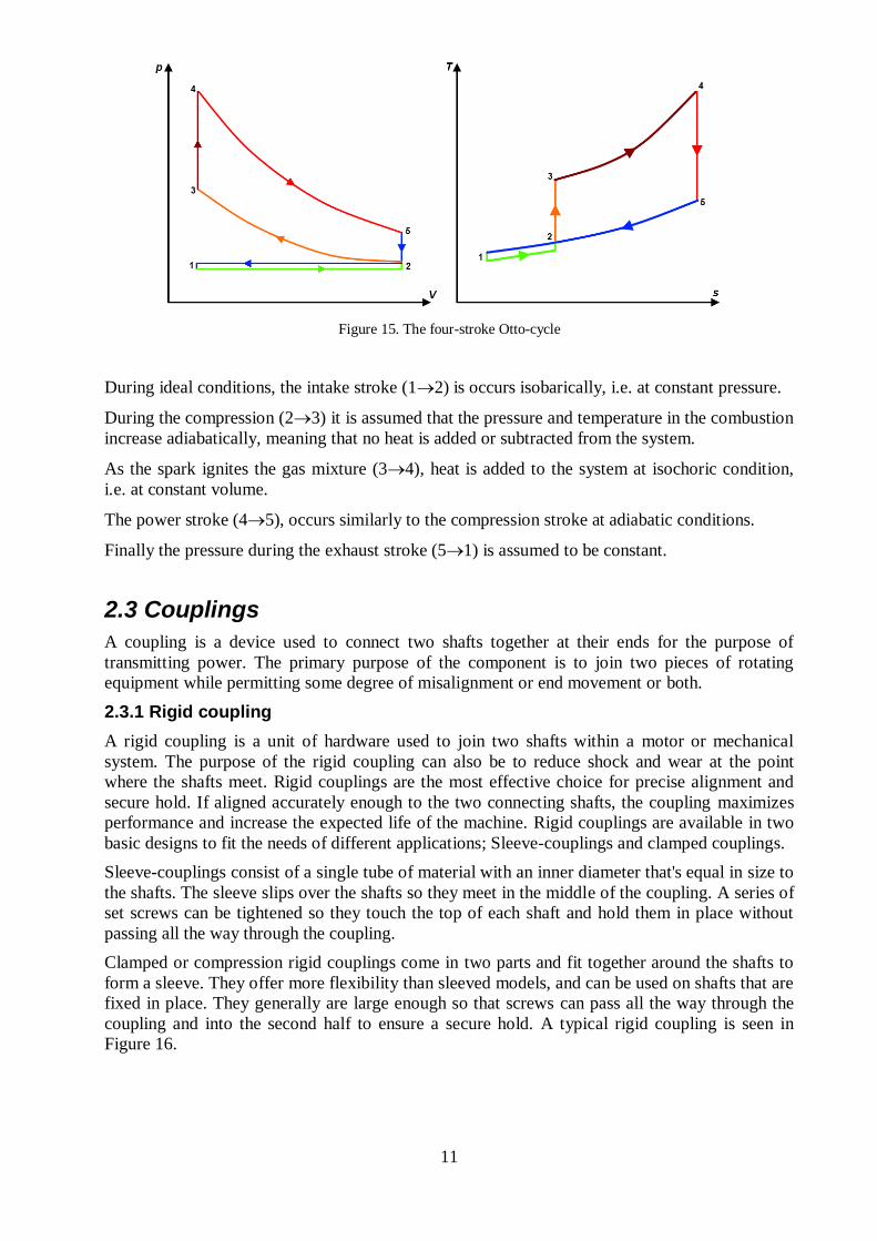
The spark ignited engine cycle, often referred to as the SI-cycle or the Otto, explained can be

modeled as a thermodynamic closed system, where each mode or stroke is expressed by a

thermodynamic process. Figure 15 illustrates the en a both a pressure-volume diagram and a

temperature-enthalpy diagram.

11

Figure 15. The four-stroke Otto-cycle

During ideal conditions, the intake stroke (12) is occurs isobarically, i.e. at constant pressure.

During the compression (23) it is assumed that the pressure and temperature in the combustion

increase adiabatically, meaning that no heat is added or subtracted from the system.

As the spark ignites the gas mixture (34), heat is added to the system at isochoric condition,

i.e. at constant volume.

The power stroke (45), occurs similarly to the compression stroke at adiabatic conditions.

Finally the pressure during the exhaust stroke (51) is assumed to be constant.

2.3 Couplings

A coupling is a device used to connect two shafts together at their ends for the purpose of

transmitting power. The primary purpose of the component is to join two pieces of rotating

equipment while permitting some degree of misalignment or end movement or both.

2.3.1 Rigid coupling

A rigid coupling is a unit of hardware used to join two shafts within a motor or mechanical

system. The purpose of the rigid coupling can also be to reduce shock and wear at the point

where the shafts meet. Rigid couplings are the most effective choice for precise alignment and

secure hold. If aligned accurately enough to the two connecting shafts, the coupling maximizes

performance and increase the expected life of the machine. Rigid couplings are available in two

basic designs to fit the needs of different applications; Sleeve-couplings and clamped couplings.

Sleeve-couplings consist of a single tube of material with an inner diameter that's equal in size to

the shafts. The sleeve slips over the shafts so they meet in the middle of the coupling. A series of

set screws can be tightened so they touch the top of each shaft and hold them in place without

passing all the way through the coupling.

Clamped or compression rigid couplings come in two parts and fit together around the shafts to

form a sleeve. They offer more flexibility than sleeved models, and can be used on shafts that are

fixed in place. They generally are large enough so that screws can pass all the way through the

coupling and into the second half to ensure a secure hold. A typical rigid coupling is seen in

Figure 16.

12

Figure 16. A rigid coupling together with a schematic sketch of the coupling

2.3.2 Torsional couplings

Torsional couplings are a type of coupling designed to transfer large torques between the two

connecting shafts. Torsional couplings are divided into two groups: Torsional stiff and torsional

rigid couplings. As the names imply, the difference between the two is the amount of stiffness

each coupling provides. Torsional flexible coupling typically has a lower stiffness which allows

for a higher angular displacement during rotation. Torsional stiff couplings are designed to

minimize these angular displacements and therefore have a higher rotational stiffness.

In either case, torsional couplings are mostly designed using a rubber element to transmit torque

between two hubs. The rubber damps any vibrations moving from one shaft to the other. See

Figure 17 for an example of a typical torsion coupling.

Figure 17. Torsional coupling

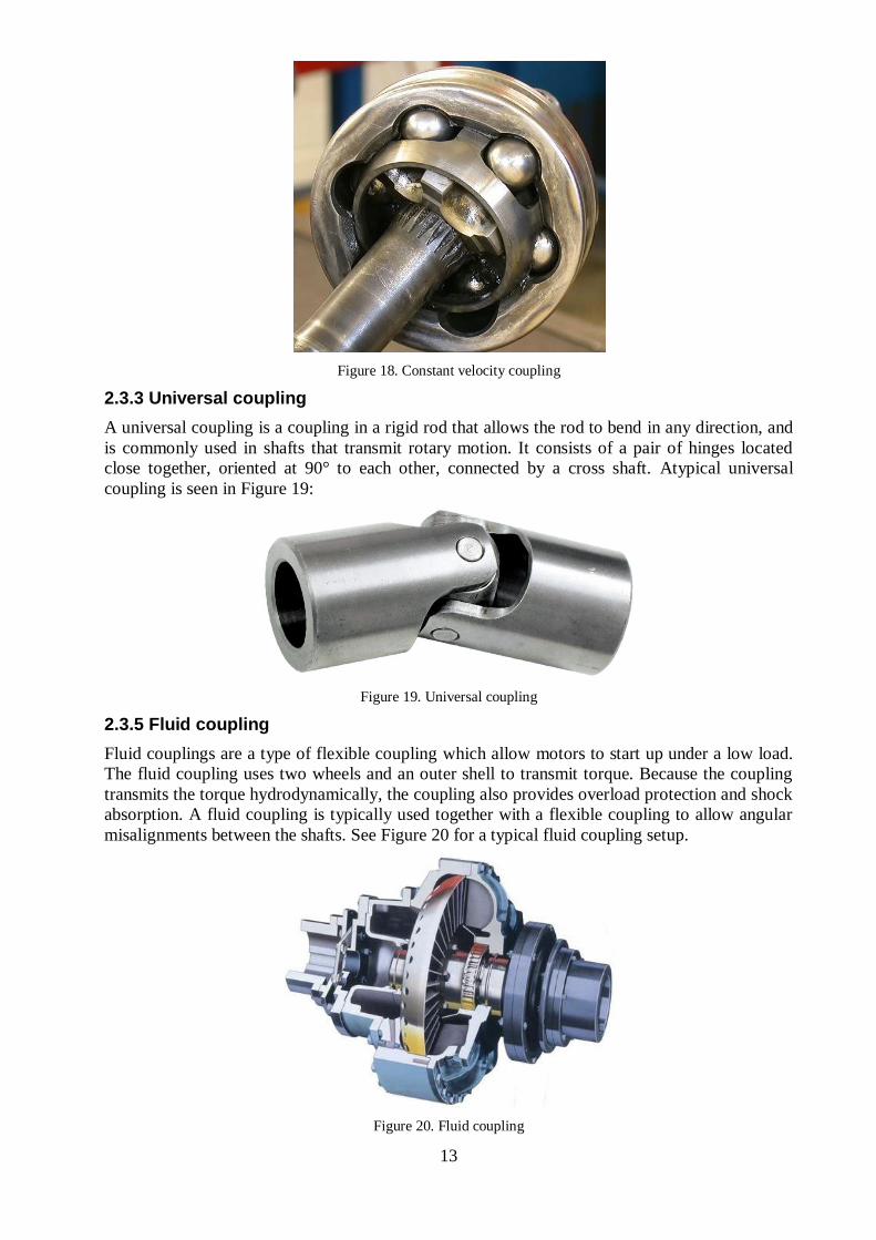
2.3.4 Constant velocity coupling

Constant-velocity couplings allow a drive shaft to transmit power through a variable angle, at

constant rotational speed. They are mainly used in front wheel drive and all wheel drive cars.

Constant-velocity joints are protected by a rubber boot, a gaiter. Cracks and splits in the boot

will allow contaminants in, which would cause the joint to wear quickly. A constant velocity

coupling of rzeppa-type is seen in Figure 18.

13

Figure 18. Constant velocity coupling

2.3.3 Universal coupling

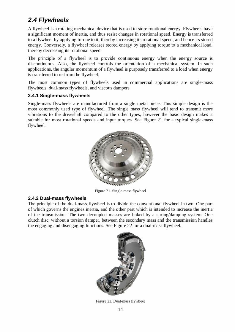
A universal coupling is a coupling in a rigid rod that allows the rod to bend in any direction, and

is commonly used in shafts that transmit rotary motion. It consists of a pair of hinges located

close together, oriented at 90° to each other, connected by a cross shaft. Atypical universal

coupling is seen in Figure 19:

Figure 19. Universal coupling

2.3.5 Fluid coupling

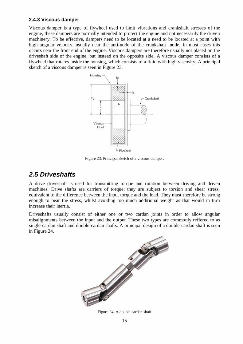
Fluid couplings are a type of flexible coupling which allow motors to start up under a low load.

The fluid coupling uses two wheels and an outer shell to transmit torque. Because the coupling

transmits the torque hydrodynamically, the coupling also provides overload protection and shock

absorption. A fluid coupling is typically used together with a flexible coupling to allow angular

misalignments between the shafts. See Figure 20 for a typical fluid coupling setup.

Figure 20. Fluid coupling

14

2.4 Flywheels

A flywheel is a rotating mechanical device that is used to store rotational energy. Flywheels have

a significant moment of inertia, and thus resist changes in rotational speed. Energy is transferred

to a flywheel by applying torque to it, thereby increasing its rotational speed, and hence its stored

energy. Conversely, a flywheel releases stored energy by applying torque to a mechanical load,

thereby decreasing its rotational speed.

The principle of a flywheel is to provide continuous energy when the energy source is

discontinuous. Also, the flywheel controls the orientation of a mechanical system. In such

applications, the angular momentum of a flywheel is purposely transferred to a load when energy

is transferred to or from the flywheel.

The most common types of flywheels used in commercial applications are single-mass

flywheels, dual-mass flywheels, and viscous dampers.

2.4.1 Single-mass flywheels

Single-mass flywheels are manufactured from a single metal piece. This simple design is the

most commonly used type of flywheel. The single mass flywheel will tend to transmit more

vibrations to the driveshaft compared to the other types, however the basic design makes it

suitable for most rotational speeds and input torques. See Figure 21 for a typical single-mass

flywheel.

Figure 21. Single-mass flywheel

2.4.2 Dual-mass flywheels The principle of the dual-mass flywheel is to divide the conventional flywheel in two. One part

of which governs the engines inertia, and the other part which is intended to increase the inertia

of the transmission. The two decoupled masses are linked by a spring/damping system. One

clutch disc, without a torsion damper, between the secondary mass and the transmission handles

the engaging and disengaging functions. See Figure 22 for a dual-mass flywheel.

Figure 22. Dual-mass flywheel

15

2.4.3 Viscous damper

Viscous damper is a type of flywheel used to limit vibrations and crankshaft stresses of the

engine, these dampers are normally intended to protect the engine and not necessarily the driven

machinery, To be effective, dampers need to be located at a need to be located at a point with

high angular velocity, usually near the anti-node of the crankshaft mode. In most cases this

occurs near the front end of the engine. Viscous dampers are therefore usually not placed on the

driveshaft side of the engine, but instead on the opposite side. A viscous damper consists of a

flywheel that rotates inside the housing, which consists of a fluid with high viscosity. A principal

sketch of a viscous damper is seen in Figure 23.

Figure 23. Principal sketch of a viscous damper.

2.5 Driveshafts

A drive driveshaft is used for transmitting torque and rotation between driving and driven

machines. Drive shafts are carriers of torque: they are subject to torsion and shear stress,

equivalent to the difference between the input torque and the load. They must therefore be strong

enough to bear the stress, whilst avoiding too much additional weight as that would in turn

increase their inertia.

Driveshafts usually consist of either one or two cardan joints in order to allow angular

misalignments between the input and the output. These two types are commonly reffered to as

single-cardan shaft and double-cardan shafts. A principal design of a double-cardan shaft is seen

in Figure 24.

Figure 24. A double cardan shaft

16

2.6 Torque sensors

Torques can be divided into two major categories, static and dynamic. Depending on which type

is desired to be measured, certain measurement techniques are more appropriate than others. As

the test bed exerts both static and dynamic torques during operation, special considerations must

be made when determining how best to measure it.

The methods for measuring torque are also divided into two categories: reaction measurements

and in-line measurements.

In-line torque measurements are made by inserting a torque sensor between torque carrying

components, this method allows the torque sensor to be placed as close as possible to the torque

of interest and avoid possible errors in the measurements.

A reaction torque sensor takes advantage of reaction forces. To measure the torque produced by

the engine, the reaction torque is required to prevent the motor from turning would be measured.

Reaction measurements avoid the problem of making the electrical connection to the sensor in a

rotating application, but do come with drawbacks. A reaction torque sensor is often required to

carry significant extraneous loads, for instance as the weight of an electric motor [2].

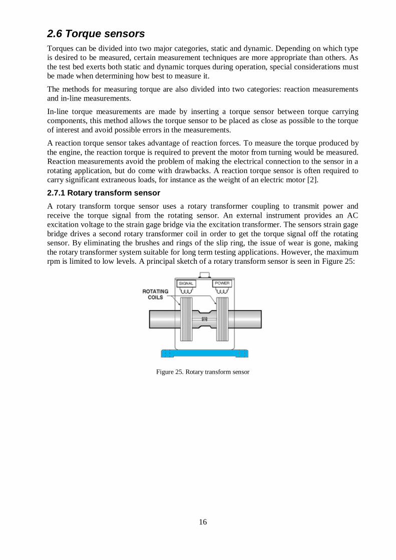
2.7.1 Rotary transform sensor

A rotary transform torque sensor uses a rotary transformer coupling to transmit power and

receive the torque signal from the rotating sensor. An external instrument provides an AC

excitation voltage to the strain gage bridge via the excitation transformer. The sensors strain gage

bridge drives a second rotary transformer coil in order to get the torque signal off the rotating

sensor. By eliminating the brushes and rings of the slip ring, the issue of wear is gone, making

the rotary transformer system suitable for long term testing applications. However, the maximum

rpm is limited to low levels. A principal sketch of a rotary transform sensor is seen in Figure 25:

Figure 25. Rotary transform sensor

17

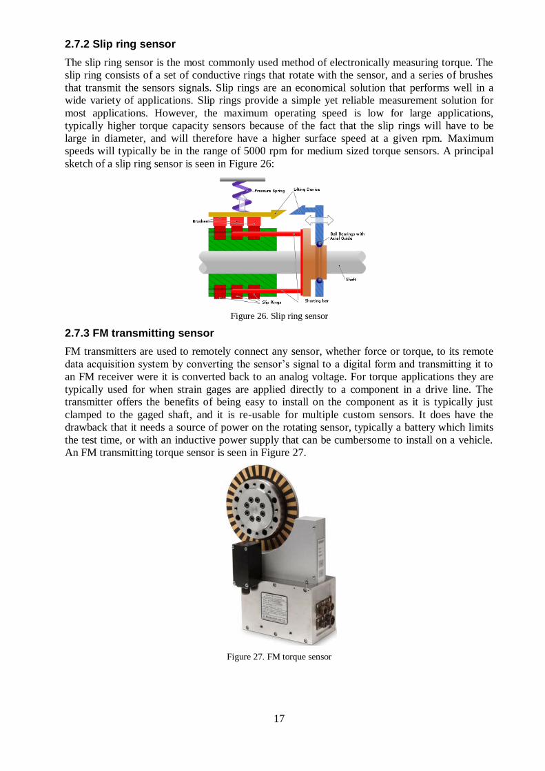
2.7.2 Slip ring sensor

The slip ring sensor is the most commonly used method of electronically measuring torque. The

slip ring consists of a set of conductive rings that rotate with the sensor, and a series of brushes

that transmit the sensors signals. Slip rings are an economical solution that performs well in a

wide variety of applications. Slip rings provide a simple yet reliable measurement solution for

most applications. However, the maximum operating speed is low for large applications,

typically higher torque capacity sensors because of the fact that the slip rings will have to be

large in diameter, and will therefore have a higher surface speed at a given rpm. Maximum

speeds will typically be in the range of 5000 rpm for medium sized torque sensors. A principal

sketch of a slip ring sensor is seen in Figure 26:

Figure 26. Slip ring sensor

2.7.3 FM transmitting sensor

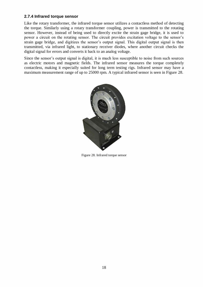
FM transmitters are used to remotely connect any sensor, whether force or torque, to its remote

data acquisition system by converting the sensor’s signal to a digital form and transmitting it to

an FM receiver were it is converted back to an analog voltage. For torque applications they are

typically used for when strain gages are applied directly to a component in a drive line. The

transmitter offers the benefits of being easy to install on the component as it is typically just

clamped to the gaged shaft, and it is re-usable for multiple custom sensors. It does have the

drawback that it needs a source of power on the rotating sensor, typically a battery which limits

the test time, or with an inductive power supply that can be cumbersome to install on a vehicle.

An FM transmitting torque sensor is seen in Figure 27.

Figure 27. FM torque sensor

18

2.7.4 Infrared torque sensor

Like the rotary transformer, the infrared torque sensor utilizes a contactless method of detecting

the torque. Similarly using a rotary transformer coupling, power is transmitted to the rotating

sensor. However, instead of being used to directly excite the strain gage bridge, it is used to

power a circuit on the rotating sensor. The circuit provides excitation voltage to the sensor’s

strain gage bridge, and digitizes the sensor’s output signal. This digital output signal is then

transmitted, via infrared light, to stationary receiver diodes, where another circuit checks the

digital signal for errors and converts it back to an analog voltage.

Since the sensor’s output signal is digital, it is much less susceptible to noise from such sources

as electric motors and magnetic fields. The infrared sensor measures the torque completely

contactless, making it especially suited for long term testing rigs. Infrared sensor may have a

maximum measurement range of up to 25000 rpm. A typical infrared sensor is seen in Figure 28.

Figure 28. Infrared torque sensor

19

3 ANALYSIS & DIMENSIONING

This chapter describes the methods used to analyze and dimension the test bed components.

3.1 Engine torque dynamics

The torque Te produced by the engine is the sum of a number of different torque components

(1)

where Tmass is the torque produced by the oscillating and reciprocating motion of the piston; Tin is

the torque produced during the intake of air in the piston chamber; Tcomp is the torque produced

during the compression stroke, when the air/fuel mixture is compressed inside the cylinder; Tcomb

is the torque produced by the ignition of the fuel in the piston chamber; Texp is the torque

produced during the power-stroke, when the expansion of the hot gas from the combustion is

forcing the piston down; Texh is the torque subtracted during the exhaust stroke, when the piston

is venturing the residual gases from the chamber; Tfric is total frictional losses due to friction

between the piston and cylinder walls etc.

The useful output torque is created by the combustion, power-stroke, blow-down intake pressure,

and the momentum created by the inertia, while the compression, exhaust back pressure and

friction between piston and cylinder walls are considered as losses to the output torque. The

positive and negative components are summarized in Table 1:

Table 1. Torque component

Torque component Sign

Tin +

Tmass +/-

Tcomp -

Tcomb +

Texp +

Texh -

-

The torque components are analyzed in the following paragraphs:

20

3.1.1 Mass torque

The mass torque is created as a result of the inertial forces exerted by the motions of the piston,

connecting rod and crankshaft. A principal sketch of these components is seen in Figure 29:

Figure 29. Principal sketch of the piston, connecting rod and crankshaft

The vertical position xp of the piston is given by:

( ) ( ) (2)

where rcrank is the crankshaft radius, is the crank angle degree, lrod is the length of the

connecting rod, is the angle adjacent to the crankshaft radius.

The following trigonometric relationship exists between the angles and :

(3)

Solving equation (2) for theta gives:

(4)

The Pythagorean trigonometric identity gives:

(5)

Solving equation (5) for cos and inserting equation (4) gives:

√ √ (

)

(6)

Inserting equation (6) into equation (1) gives:

( ) ( √ (

)

) (7)

21

Rewriting equation (7) gives:

(

√ (

)

) (8)

In order to simplify the expression, the ratio between crankshaft radius and the connecting rod

length is used:

(9)

The crank angle is expressed as a function of the angular velocity and the time t:

(10)

where the following relationship exists between the angular velocity and the speed n.

(11)

Inserting equations (9) and (10) into (8) gives:

(( )

( √ ( ) )) (12)

The vertical velocity vp of the piston is the time derivative of xp:

(

√ ( ) ) (13)

The vertical acceleration ap of the piston is the 2nd

time derivative of xp:

(

√ ( )

(√ ( ) ) ) (14)

The first part of equation (14), simply involving the cost term, is referred to as the first-order

inertial acceleration; and the remaining part, dependent on the ratio , represent the inertial

forces of order 2nd

, 4th etc. As equation (14) shows, a value of close to zero would result in that

the multi-order free forces would be omitted completely. An infinitely small -value would

however require an infinitely long connecting rod. This illustrates the fact that a small ratio

between the crank radius and rod length is beneficial for the reduction of the inertial vibration in

a reciprocating engine [3].

The single cylinder engine has a connecting rod length of 156.5 mm and crankshaft radius of

47.3 mm, resulting in a -value of 0.3.

The position, velocity and acceleration over a full combustion cycle are illustrated in Figure 30:

22

Figure 30. Piston position, velocity and acceleration during one engine cycle.

The oscillating accelerations of the piston results in a likewise oscillating piston force Fp, which

is converted through the connecting rod into a rotational force Ft force, tangential to the

crankshaft [4]. A free-body diagram of the forces acting on the piston, connecting rod and

crankshaft is shown in Figure 31:

Figure 31. Free body diagram of forces in the piston, connecting rod and crankshaft

The piston force Fp is defined as:

(15)

where mp is the piston mass, 0.987 kg. The contact force FW between the piston and the chamber

walls is defined as:

(16)

where μ is the friction coefficient between the piston and the cylinder wall, as the contact area

between piston and cylinder is kept lubricated, the friction coefficient is assumed to be small

enough that the wall force may be negliable.

23

The reciprocating-oscillating force Fh in the connecting rod is defined as a function of the piston

acceleration and mass:

(17)

The centrifugal force Fc of the crankshaft is defined as:

(18)

where mcrank is the mass of the crankshafts rotating part. The tangential force Ft is defined as:

( ) (19)

The equation is rewritten using equation (6) in (19):

(

√ ( ) ) (20)

The oscillating and tangential forces are illustrated in Figure 32:

Figure 32. Piston and crankshaft forces during one engine revolution

The mass torque Tmass is proportional to the tangential force:

(21)

24

The mass torque is illustrated in Figure 33:

Figure 33. The mass torque over one engine cycle

As seen in the figure, a positive mass torque is exerted as the piston moves downwards, and a

negative torque is exerted as to piston is forced upwards.

3.1.2 Compression & expansion torque

The compression and expansion torques are the results of the forces exerted by the compression

and expansion of the gas mixture in the combustion chamber. This is represented by the upper

half of the Otto cycle, see Figure 34:

Figure 34. Pressure-volume diagram of an ideal Otto cycle.

The compression of the fuel and air gas mixture (2-3) is assumed to be adiabatic, meaning that

no additional heat is added or rejected [5]. The adiabatic equilibrium between two states is given

by:

(22)

where p1 and p2 are the pressures at closing of the intake valve and the end of compression

respectively, V1 is the volume at BDC, V2 is the volume at TDC, is the specific heat ratio.

(23)

25

Rewriting equation (23) for the compression pressure gives:

(

)

(24)

Similarly during the power stroke (4-5), the expansion of the hot gas mixture is assumed to be

adiabatic, given by the equilibrium:

(25)

Rewriting equation (25) for the expansion pressure gives:

(

)

(26)

The cylinder volume V is a function of the piston position and area:

(

( )

( √ ( ) )) (27)

where Acyl is the cylinder area, ε is the compression ratio. The cylinder area is determined by:

(28)

where dp is the diameter of the piston.

The compression and expansion of the gas creates a horizontal force proportional to the pressure:

(29)

(30)

Similarly to the mass torque, the torque produced compression and expansion is perpendicular to

the crankshaft motion:

(

√ ( ) ) (31)

(

√ ( ) ) (32)

26

The compression and expansion torque is illustrated in Figure 35.

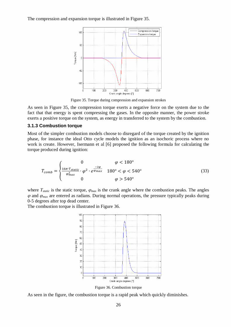
Figure 35. Torque during compression and expansion strokes

As seen in Figure 35, the compression torque exerts a negative force on the system due to the

fact that that energy is spent compressing the gases. In the opposite manner, the power stroke

exerts a positive torque on the system, as energy in transferred to the system by the combustion.

3.1.3 Combustion torque

Most of the simpler combustion models choose to disregard of the torque created by the ignition

phase, for instance the ideal Otto cycle models the ignition as an isochoric process where no

work is create. However, Isermann et al [6] proposed the following formula for calculating the

torque produced during ignition:

{

(33)

where Tstatic is the static torque, max is the crank angle where the combustion peaks. The angles

and max are entered as radians. During normal operations, the pressure typically peaks during

0-5 degrees after top dead center.

The combustion torque is illustrated in Figure 36.

Figure 36. Combustion torque

As seen in the figure, the combustion torque is a rapid peak which quickly diminishes.

27

3.1.5 Intake and exhaust torque

The pressures in the combustion chamber during intake and exhaust strokes were measured to an

average static value of 0.78 and 1.2 bar, respectively. However as seen in Figure 37, these

pressures highly dynamic.

Figure 37. Intake and exhaust pressures

Due to the preset camshaft timings, the exhaust and intake valves close and open slightly before

and after TDC. Moreover, due to the design of the exhaust chamber, pressure pulses are created

that oscillate over the exhaust stroke. These pulses creates a back pressure to the combustion

may have a negative impact on the combustion efficiency.

3.1.6 Friction torque

The friction torque is created from the contact between the piston and the cylinder walls during

the reciprocating motion. The oil film and bushings are used to reduce the contact force,

regardless of this there will always be a friction force present between the piston and cylinder

walls.

The friction torque is difficult to both model and measure at a crank-angle resolved level, based

on measurement results it is therefore assumed that the losses in torque due to friction is roughly

10%.

3.1.7 Total torque

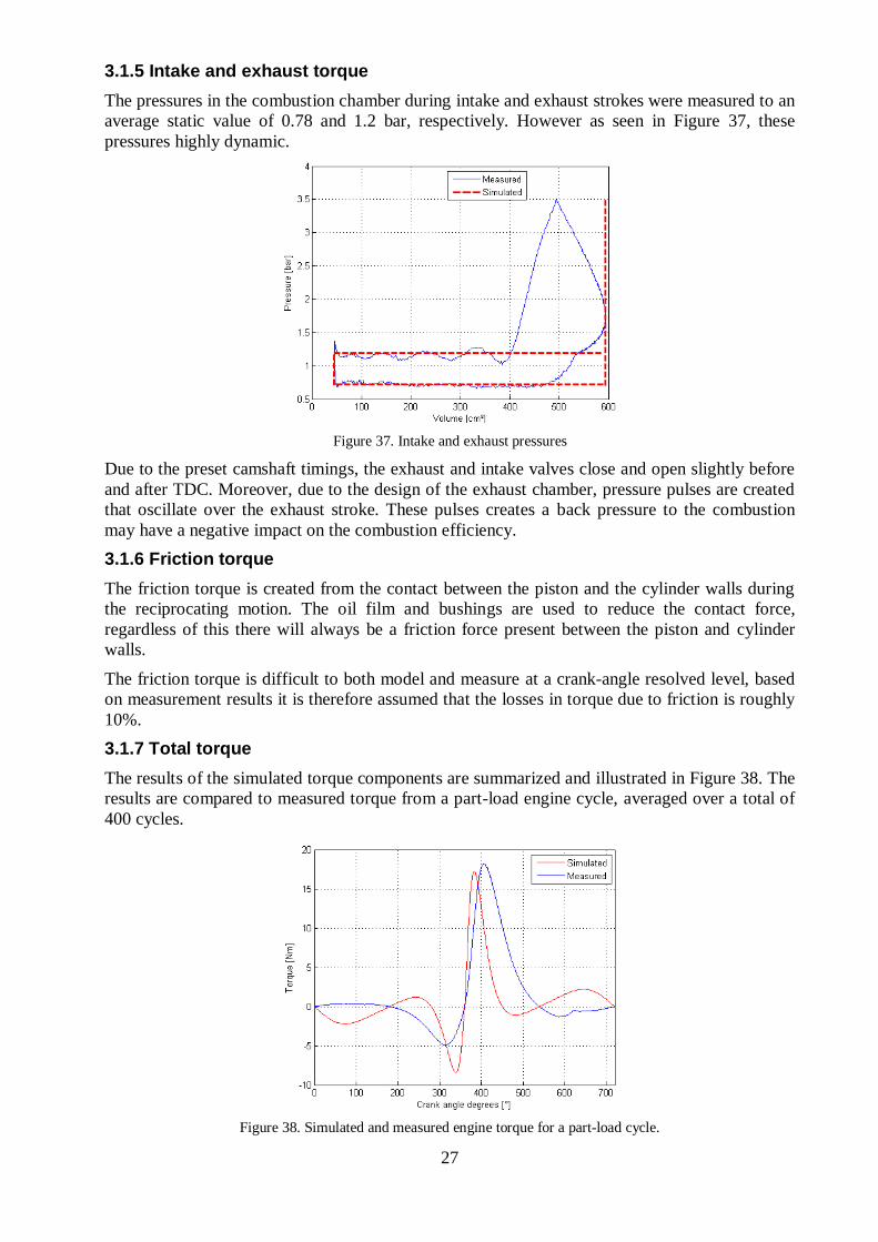
The results of the simulated torque components are summarized and illustrated in Figure 38. The

results are compared to measured torque from a part-load engine cycle, averaged over a total of

400 cycles.

Figure 38. Simulated and measured engine torque for a part-load cycle.

28

As the figure shows, the simulated results differ from the measured. Possible reasons for this are

that is that the model does not take into account heat losses during combustion and exhaust,

deviations in ignition point, burn rate etc. In order to match the simulated torque, a calibration

function is added to tune the results better to the measured. The results are shown in Figure 39.

Figure 39. Tuned simulated and measured engine torque.

The engine torque reaches a peak value once every second revolution, a peak pulse ratio of q=0.5

is therefore assumed.

29

3.2 Inertia and stiffness of components

In order to model the vibration modes of a system, it is necessary to first determine the rotational

inertia and stiffness of the subsystem components.

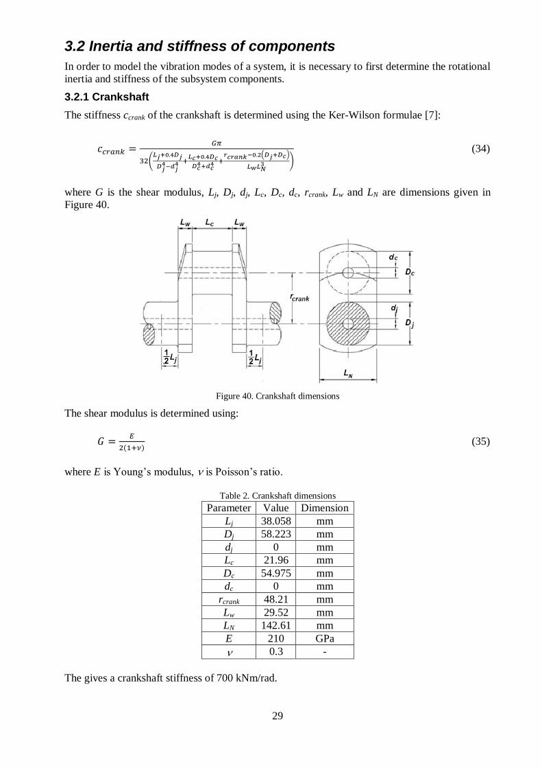
3.2.1 Crankshaft

The stiffness ccrank of the crankshaft is determined using the Ker-Wilson formulae [7]:

(

( )

)

(34)

where G is the shear modulus, Lj, Dj, dj, Lc, Dc, dc, rcrank, Lw and LN are dimensions given in

Figure 40.

Figure 40. Crankshaft dimensions

The shear modulus is determined using:

( ) (35)

where E is Young’s modulus, is Poisson’s ratio.

Table 2. Crankshaft dimensions

Parameter Value Dimension

Lj 38.058 mm

Dj 58.223 mm

dj 0 mm

Lc 21.96 mm

Dc 54.975 mm

dc 0 mm

rcrank 48.21 mm

Lw 29.52 mm

LN 142.61 mm

E 210 GPa

0.3 -

The gives a crankshaft stiffness of 700 kNm/rad.

30

The rotational inertia of the engine is given as a sum of the crankshaft inertia and the inertia of

the rotating part of the connecting rod [8]:

(

( )

)

(36)

where mr is the sum of the rotating masses and mo is the sum of the oscillating masses. Usually

the connecting rod is considered to have a 2/3 rotating and 1/3 oscillating part:

(37)

(38)

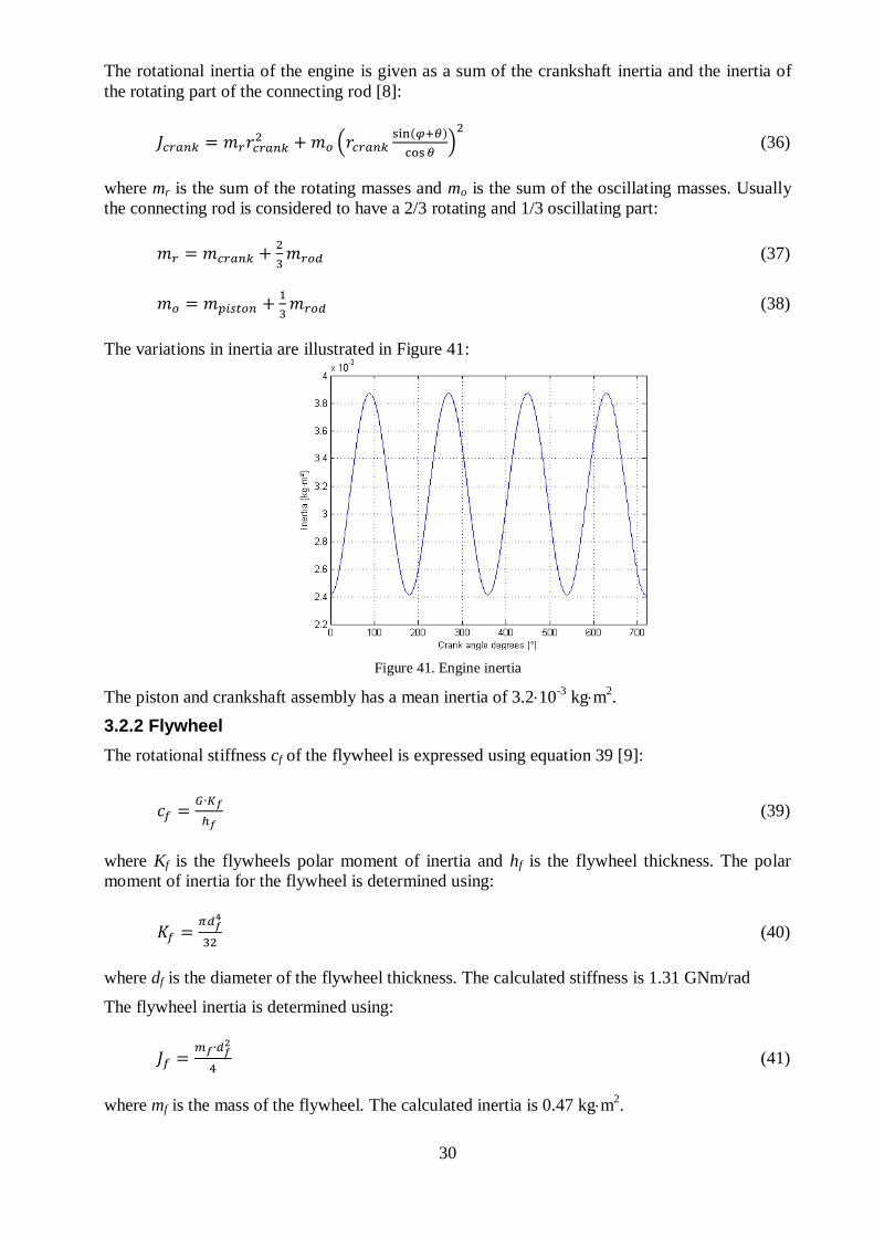
The variations in inertia are illustrated in Figure 41:

Figure 41. Engine inertia

The piston and crankshaft assembly has a mean inertia of 3.210-3

kgm2.

3.2.2 Flywheel

The rotational stiffness cf of the flywheel is expressed using equation 39 [9]:

(39)

where Kf is the flywheels polar moment of inertia and hf is the flywheel thickness. The polar

moment of inertia for the flywheel is determined using:

(40)

where df is the diameter of the flywheel thickness. The calculated stiffness is 1.31 GNm/rad

The flywheel inertia is determined using:

(41)

where mf is the mass of the flywheel. The calculated inertia is 0.47 kgm2.

31

3.2.3 Couplings

The stiffness and inertia of the coupling are determined using equations (39) and (41) with

corresponding physical parameters. The stiffness and inertia of the couplings is 152 MNm/rad

and 0.139 kgm2, respectively.

3.2.4 Driveshaft

The rotational stiffness cd of the driveshaft is determined by:

(42)

where Kf is the flywheels polar moment of inertia and hf is the flywheel thickness. The stiffness

is determined to 521 kNm/rad.

The driveshaft inertia is determined to 1.7210-2

kgm2.

3.2.5 Electric motor

According to data sheets from the manufacturer, the motor has a rotational stiffness 2.45

GNm/rad and a moment of inertia of 2.1 kgm2.

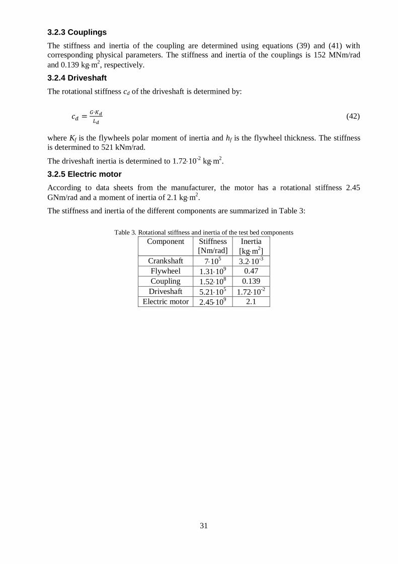
The stiffness and inertia of the different components are summarized in Table 3:

Table 3. Rotational stiffness and inertia of the test bed components

Component Stiffness

[Nm/rad]

Inertia

[kgm2]

Crankshaft 7105 3.210

-3

Flywheel 1.31109 0.47

Coupling 1.52108 0.139

Driveshaft 5.21105 1.7210

-2

Electric motor 2.45109 2.1

32

3.3 Resonance frequencies and critical speeds

Torsional vibrations occur in a rotor when the rotational interference has a frequency such that

the rotor is subjected to resonance. The interference frequency is usually related to the rotor

speed in a known way, at which point it is necessary to determine the rotational speed which lead

to the interference frequency which makes the rotor come in resonance. This is known as a

critical speed.

Bending critical speeds could also be achieved by exciting with general interference frequencies,

but in that case there are always interference frequencies that are consistent with the rotational

frequency due to the imbalance of the rotational mass. Corresponding disturbances are not

present for torsional vibrations, at least lot for vertical rotors. For horizontal rotors, the

gravitational field will create one disturbance per revolution [10].

Before calculating the critical speeds, the disturbance frequencies must be identified and their

frequency-speed relationship determined.

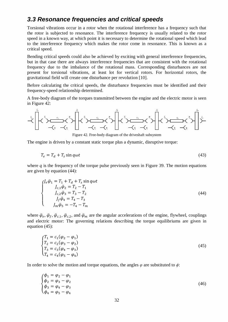
A free-body diagram of the torques transmitted between the engine and the electric motor is seen

in Figure 42:

Figure 42. Free-body diagram of the driveshaft subsystem

The engine is driven by a constant static torque plus a dynamic, disruptive torque:

(43)

where q is the frequency of the torque pulse previously seen in Figure 39. The motion equations

are given by equation (44):

{

(44)

where , , , , and are the angular accelerations of the engine, flywheel, couplings

and electric motor: The governing relations describing the torque equilibriums are given in

equation (45):

{

( )

( )

( )

( )

(45)

In order to solve the motion and torque equations, the angles φ are substituted to ϕ:

{

(46)

33

Equations (45) and (46) in (44) gives, after rewriting, a set of four 2nd

order differential

equations:

{

(47)

Equation (47) is rewritten in matrix form:

[

]

[

]

[

]

[

] (48)

Equation (47) is rewritten in matrix form:

(49)

Equation (49) is solved for the critical speeds cr which theoretically give infinite values for ϕ

there by infinite resonance to the system. The solution is given by:

{

√ (

)

√ (

)

√ (

)

√ (

)

(50)

As observed in equation (50), the critical speeds that generate large resonances to the system is

governed by the stiffness of the engine, flywheel, couplings and electric motor; and the stiffness

of their connections; i.e. the driveshaft. In order to achieve a high limit for a critical system

speed, it is therefore necessary the components are dimensioned with a low enough inertia and

high enough stiffness.

Since the optimization strategy is based on increasing the increasing the limit of the critical

speed over 6000 rpm, the critical speed of interest for the system analysis is the minimum of the

four. The overall critical speed of the system is thus given by:

( ) (51)

As previously mentioned, the flywheel stands for a substantial part of the total system inertia.

34

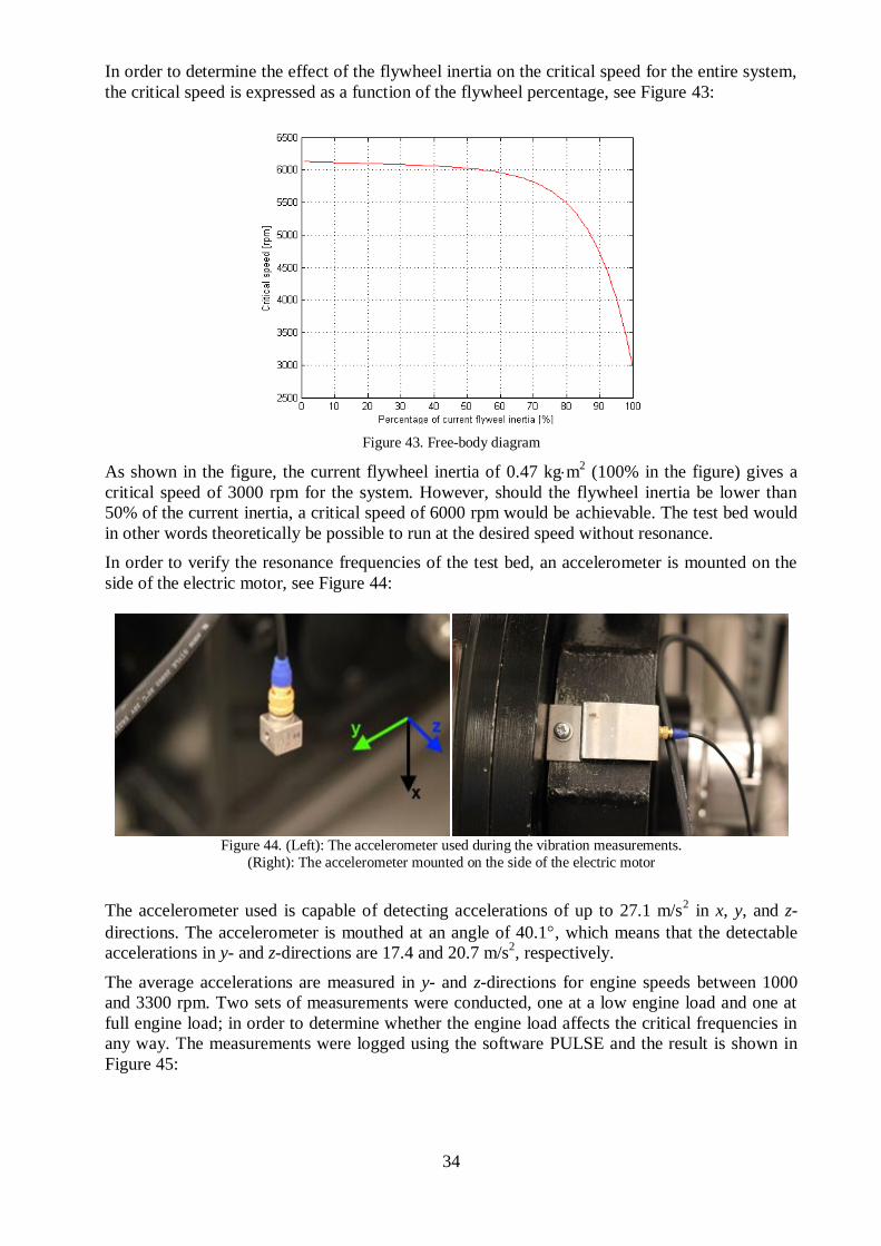
In order to determine the effect of the flywheel inertia on the critical speed for the entire system,

the critical speed is expressed as a function of the flywheel percentage, see Figure 43:

Figure 43. Free-body diagram

As shown in the figure, the current flywheel inertia of 0.47 kgm2 (100% in the figure) gives a

critical speed of 3000 rpm for the system. However, should the flywheel inertia be lower than

50% of the current inertia, a critical speed of 6000 rpm would be achievable. The test bed would

in other words theoretically be possible to run at the desired speed without resonance.

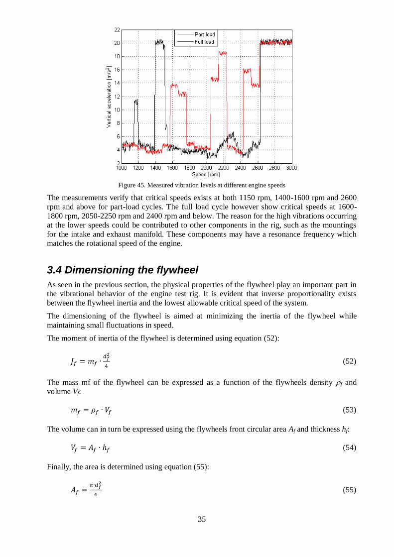
In order to verify the resonance frequencies of the test bed, an accelerometer is mounted on the

side of the electric motor, see Figure 44:

Figure 44. (Left): The accelerometer used during the vibration measurements.

(Right): The accelerometer mounted on the side of the electric motor

The accelerometer used is capable of detecting accelerations of up to 27.1 m/s2 in x, y, and z-

directions. The accelerometer is mouthed at an angle of 40.1, which means that the detectable

accelerations in y- and z-directions are 17.4 and 20.7 m/s2, respectively.

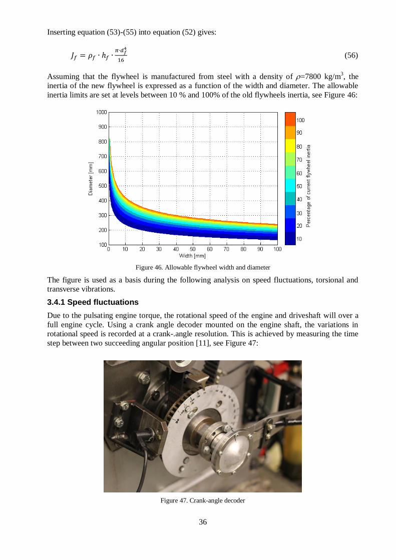
The average accelerations are measured in y- and z-directions for engine speeds between 1000

and 3300 rpm. Two sets of measurements were conducted, one at a low engine load and one at

full engine load; in order to determine whether the engine load affects the critical frequencies in

any way. The measurements were logged using the software PULSE and the result is shown in

Figure 45:

35

Figure 45. Measured vibration levels at different engine speeds

The measurements verify that critical speeds exists at both 1150 rpm, 1400-1600 rpm and 2600

rpm and above for part-load cycles. The full load cycle however show critical speeds at 1600-

1800 rpm, 2050-2250 rpm and 2400 rpm and below. The reason for the high vibrations occurring

at the lower speeds could be contributed to other components in the rig, such as the mountings

for the intake and exhaust manifold. These components may have a resonance frequency which

matches the rotational speed of the engine.

3.4 Dimensioning the flywheel

As seen in the previous section, the physical properties of the flywheel play an important part in

the vibrational behavior of the engine test rig. It is evident that inverse proportionality exists

between the flywheel inertia and the lowest allowable critical speed of the system.

The dimensioning of the flywheel is aimed at minimizing the inertia of the flywheel while

maintaining small fluctuations in speed.

The moment of inertia of the flywheel is determined using equation (52):

(52)

The mass mf of the flywheel can be expressed as a function of the flywheels density f and

volume Vf:

(53)

The volume can in turn be expressed using the flywheels front circular area Af and thickness hf:

(54)

Finally, the area is determined using equation (55):

(55)

36

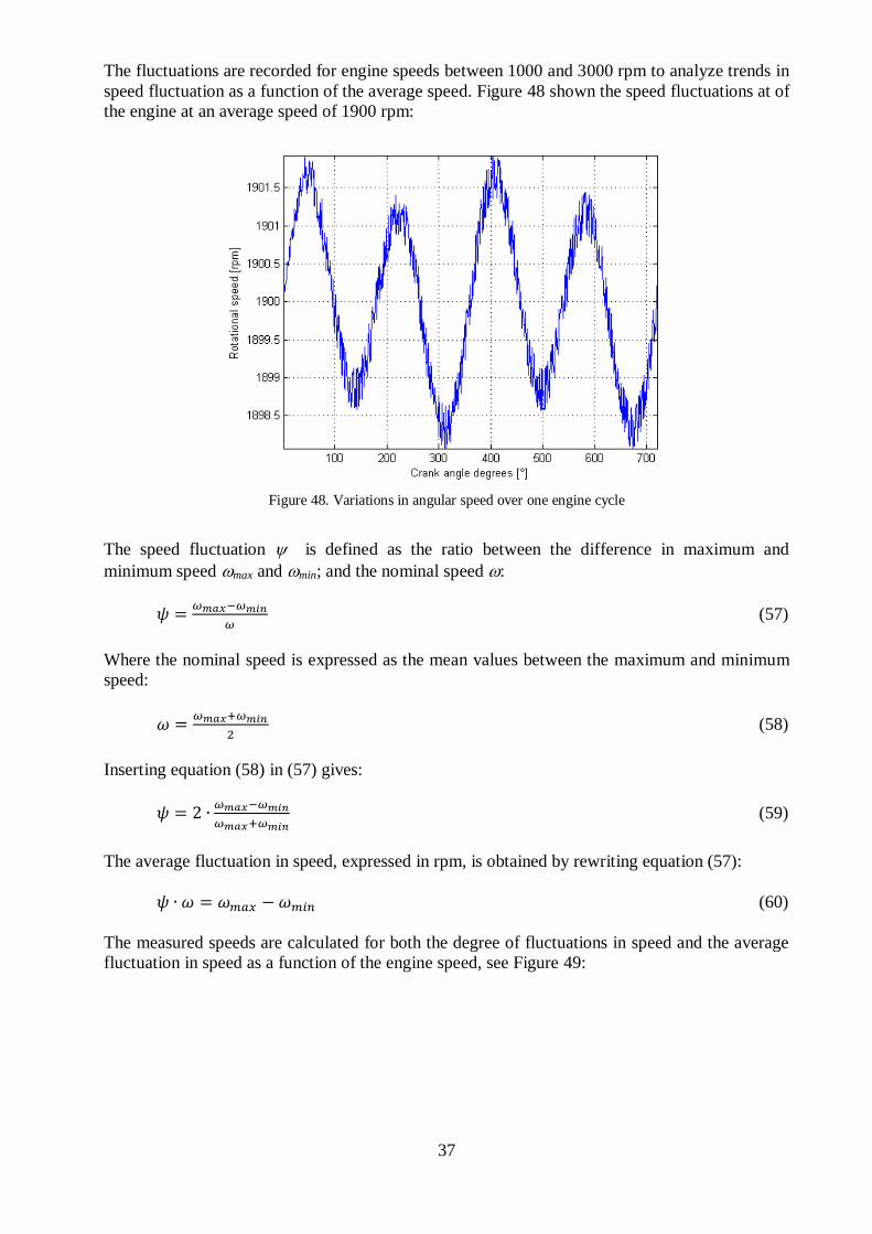
Inserting equation (53)-(55) into equation (52) gives:

(56)

Assuming that the flywheel is manufactured from steel with a density of =7800 kg/m3, the

inertia of the new flywheel is expressed as a function of the width and diameter. The allowable

inertia limits are set at levels between 10 % and 100% of the old flywheels inertia, see Figure 46:

Figure 46. Allowable flywheel width and diameter

The figure is used as a basis during the following analysis on speed fluctuations, torsional and

transverse vibrations.

3.4.1 Speed fluctuations

Due to the pulsating engine torque, the rotational speed of the engine and driveshaft will over a

full engine cycle. Using a crank angle decoder mounted on the engine shaft, the variations in

rotational speed is recorded at a crank-.angle resolution. This is achieved by measuring the time

step between two succeeding angular position [11], see Figure 47:

Figure 47. Crank-angle decoder

37

The fluctuations are recorded for engine speeds between 1000 and 3000 rpm to analyze trends in

speed fluctuation as a function of the average speed. Figure 48 shown the speed fluctuations at of

the engine at an average speed of 1900 rpm:

Figure 48. Variations in angular speed over one engine cycle

The speed fluctuation is defined as the ratio between the difference in maximum and

minimum speed max and min; and the nominal speed :

(57)

Where the nominal speed is expressed as the mean values between the maximum and minimum

speed:

(58)

Inserting equation (58) in (57) gives:

(59)

The average fluctuation in speed, expressed in rpm, is obtained by rewriting equation (57):

(60)

The measured speeds are calculated for both the degree of fluctuations in speed and the average

fluctuation in speed as a function of the engine speed, see Figure 49:

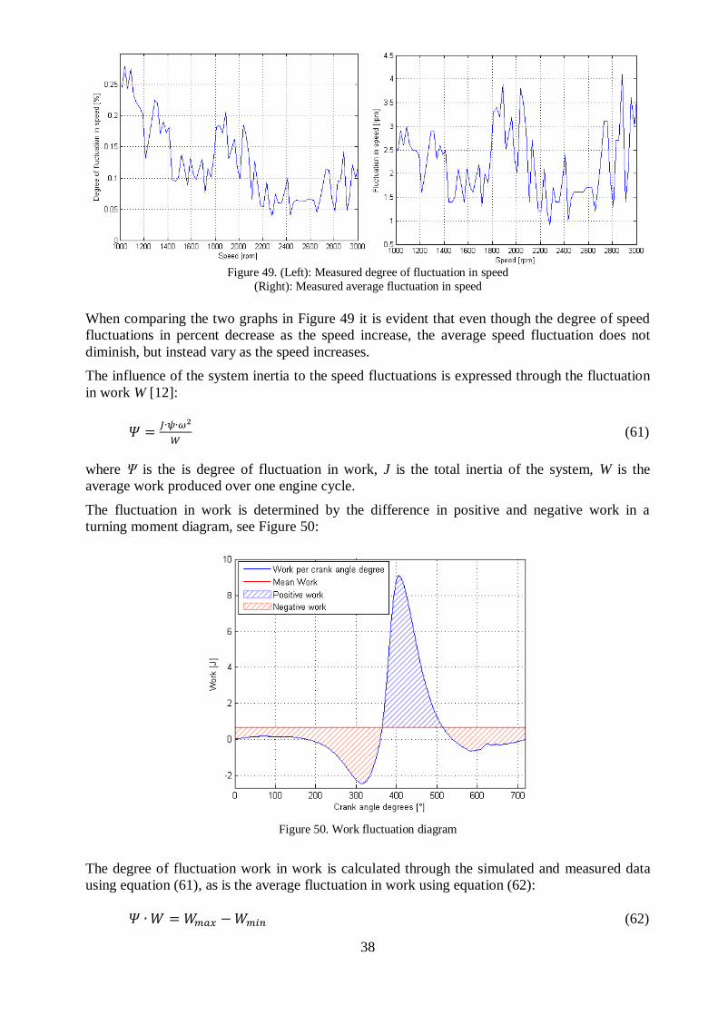
38

Figure 49. (Left): Measured degree of fluctuation in speed

(Right): Measured average fluctuation in speed

When comparing the two graphs in Figure 49 it is evident that even though the degree of speed

fluctuations in percent decrease as the speed increase, the average speed fluctuation does not

diminish, but instead vary as the speed increases.

The influence of the system inertia to the speed fluctuations is expressed through the fluctuation

in work W [12]:

(61)

where Ψ is the is degree of fluctuation in work, J is the total inertia of the system, W is the

average work produced over one engine cycle.

The fluctuation in work is determined by the difference in positive and negative work in a

turning moment diagram, see Figure 50:

Figure 50. Work fluctuation diagram

The degree of fluctuation work in work is calculated through the simulated and measured data

using equation (61), as is the average fluctuation in work using equation (62):

(62)

39

Similarly to speed fluctuations, the degree of fluctuation work as well as the average fluctuation

in work in illustrated, see Figure 51:

Figure 51. (Left): Degree of fluctuation in speed

(Right): Average fluctuation in speed

Using the measured and calculated degrees of fluctuation s in speed and work, the maximum

allowable limit for the dimensioning of the flywheel is set to a speed fluctuation of +/- 4 rpm;

and a fluctuation in work of 1250 J.

3.4.2 Torsional vibrations

As previously stated, one of the key to reduce the lateral vibrations is to lower the mass of the

flywheel. However reducing the inertia of the flywheel this causes the fluctuation in speed to

increase.

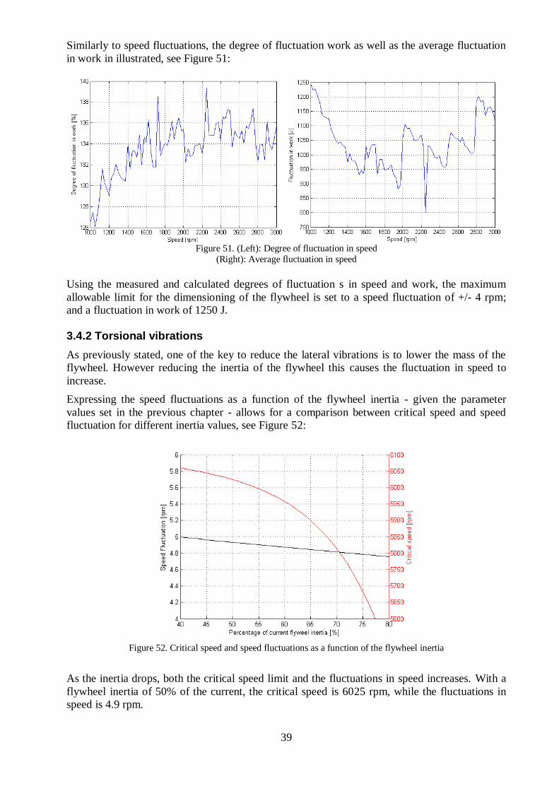
Expressing the speed fluctuations as a function of the flywheel inertia - given the parameter

values set in the previous chapter - allows for a comparison between critical speed and speed

fluctuation for different inertia values, see Figure 52:

Figure 52. Critical speed and speed fluctuations as a function of the flywheel inertia

As the inertia drops, both the critical speed limit and the fluctuations in speed increases. With a

flywheel inertia of 50% of the current, the critical speed is 6025 rpm, while the fluctuations in

speed is 4.9 rpm.

40

3.4.3 Transverse vibrations

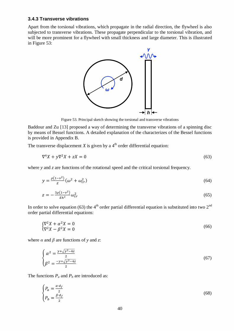
Apart from the torsional vibrations, which propagate in the radial direction, the flywheel is also

subjected to transverse vibrations. These propagate perpendicular to the torsional vibration, and

will be more prominent for a flywheel with small thickness and large diameter. This is illustrated

in Figure 53:

Figure 53. Principal sketch showing the torsional and transverse vibrations

Baddour and Zu [13] proposed a way of determining the transverse vibrations of a spinning disc

by means of Bessel functions. A detailed explanation of the characterizes of the Bessel functions

is provided in Appendix B.

The transverse displacement X is given by a 4th order differential equation:

(63)

where y and z are functions of the rotational speed and the critical torsional frequency.

( )

(

) (64)

( )

(65)

In order to solve equation (63) the 4th order partial differential equation is substituted into two 2

nd

order partial differential equations:

{

(66)

where α and β are functions of y and z:

{

√

√

(67)

The functions Pa and Pb are introduced as:

{

(68)

41

The spin-effect factor k is defined as:

√ ( )

(69)

The transverse bending stiffness of the flywheel is defined as:

( ) (70)

For a spinning disc with rotary inertia included, Pb is given by:

√(

(

)

)

(

)

(71)

The solution to equation (66) is formulated as a series of Bessel functions:

( ) ( ) ( ) ( ) ( )

( ) ( )

( ) (72)

where is the Bessel function of the first kind, is the modified Bessel function of the first

kind; and

are differentiations of the Bessel and modified Bessel functions; A11, A21, A12 and

A22 are constants given by:

{

( ) (

)

[( ) ( ( ) ) ]

[( ( )

) ( ) ]

( ) (

)

(73)

where j=1,2,3… is the mode number.

the values for Pa and Pb which satisfy both equation (71) and (73) gives the critical transverse

frequencies:

√

(74)

A numerical solution to equation (74) is possible by find the points in a graph where equations

(71) and (73) intercept. The interception points will vary with the mode number j. For the sake of

the analysis, mode number up to 6 is analyzed.

42

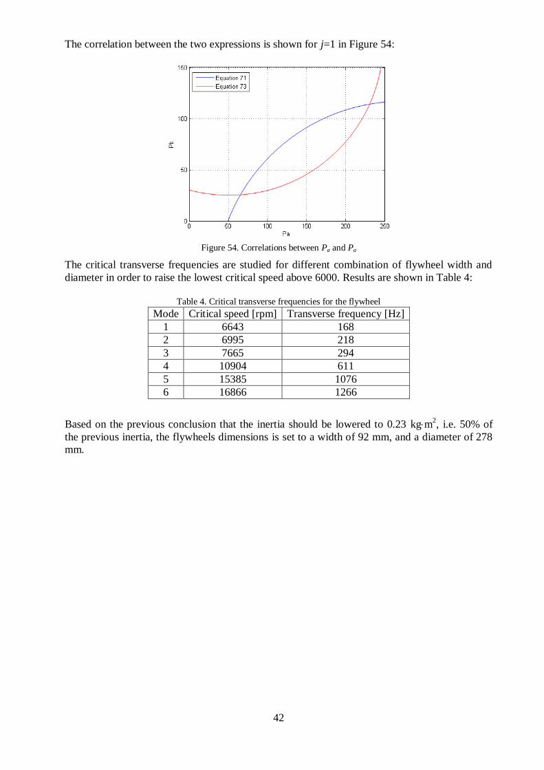
The correlation between the two expressions is shown for j=1 in Figure 54:

Figure 54. Correlations between Pa and Pa

The critical transverse frequencies are studied for different combination of flywheel width and

diameter in order to raise the lowest critical speed above 6000. Results are shown in Table 4:

Table 4. Critical transverse frequencies for the flywheel

Mode Critical speed [rpm] Transverse frequency [Hz]

1 6643 168

2 6995 218

3 7665 294

4 10904 611

5 15385 1076

6 16866 1266

Based on the previous conclusion that the inertia should be lowered to 0.23 kgm2, i.e. 50% of

the previous inertia, the flywheels dimensions is set to a width of 92 mm, and a diameter of 278

mm.

43

3.5 Dimensioning the drive shaft

The driveshaft is dimensioned to have high torsion stiffness, achieved by a diameter large

enough to withstand the shear stress as the shaft rotates at high speeds and power [14].

The shear stress τ in the shaft is given by:

(76)

where Tmax is the maximum torque produced by the engine, ds is the shaft diameter, Ks is the

polar moment of inertia for the shaft.

The shear stress τ must be lower than the yield stress τlim of the material, with the safety factor s:

(77)

The polar moment of inertia Ks is determined by equation (40): Inserting (40) and (77) in (76)

solved for the least diameter ds gives:

√

(78)

For stainless steel, the yield limit is 540 MPa. The maximum torque is 2000 Nm, the safety

factor is set to value of 1.3.

This gives a minimum shaft diameter of 39 mm. As the current shaft diameter has a diameter of

the shaft is 73 mm, a downsizing of the shaft would be a possibility.

3.6 Dimensioning the couplings

The couplings are dimensioned to have a low inertia and high torsion stiffness. The torsional

stiffness of the current coupling are 400 kNm/rad, which is a relatively high value, this however

comes as a price of a high moment of inertia.

The torsional stiffness cc of the coupling is given by:

(79)

The stiffness of the new coupling should be equal to or greater than the stiffness of the current

coupling.

(80)

The where s is a safety factor, cref is.

The moment of inertia Jc of the coupling is given by:

(81)

44

The inertia of the new coupling should be lower than or equal to the inertia of the current

coupling.

(82)

A comparison of the coupling dimensions for the least allowable stiffness and the highest

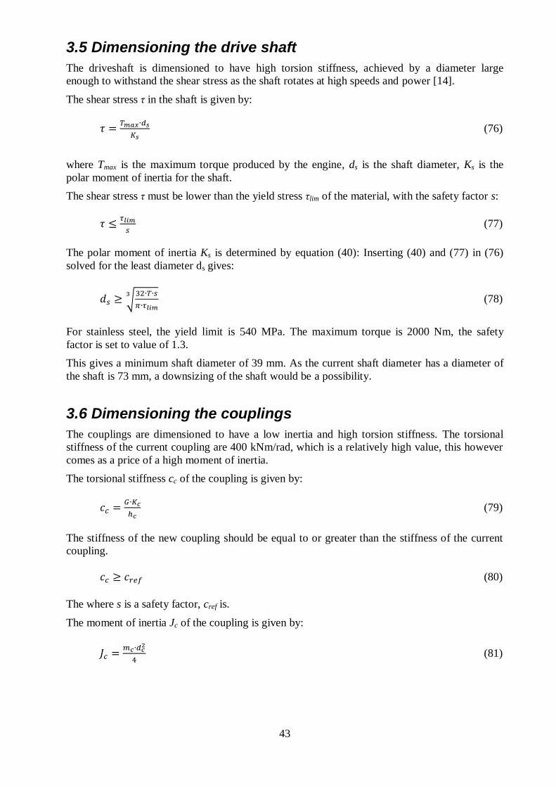
allowable inertia is seen in Figure 55:

Figure 55. Dimensions for the highest allowable inertia and the lowest allowable stiffness

The geometry of the new coupling is dimensioned to a width of 68 mm, and a diameter of 128

mm. This gives a torsional stiffness 450 kNm/rad and an inertia of 0.85 kgm2.

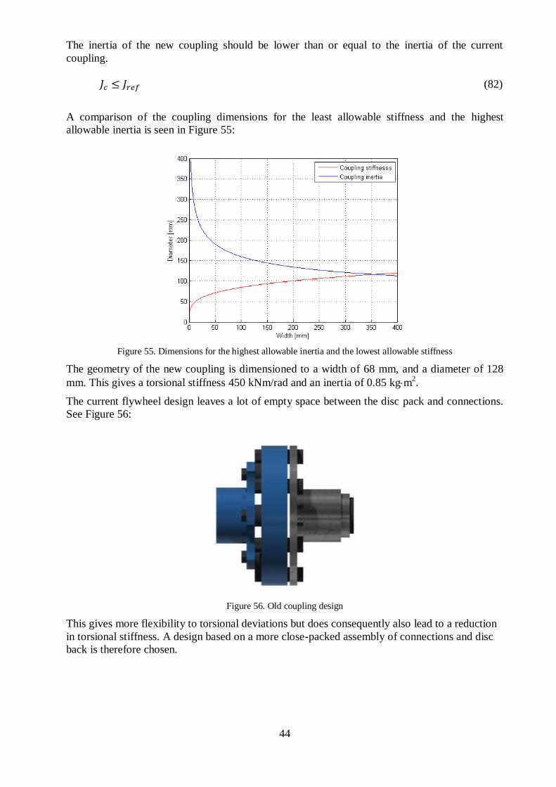
The current flywheel design leaves a lot of empty space between the disc pack and connections.

See Figure 56:

Figure 56. Old coupling design

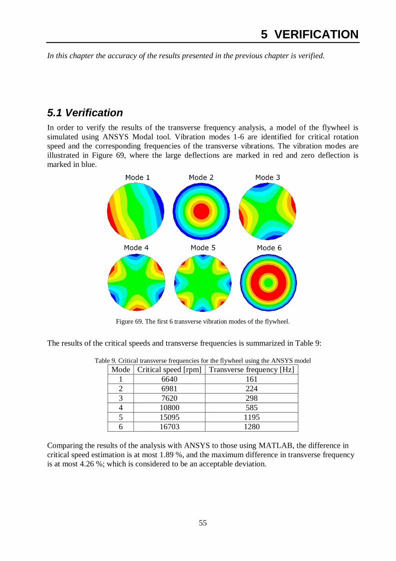
This gives more flexibility to torsional deviations but does consequently also lead to a reduction

in torsional stiffness. A design based on a more close-packed assembly of connections and disc

back is therefore chosen.

45

3.7 Dimensioning the crankshaft

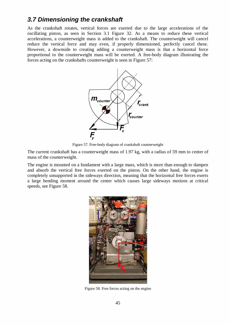
As the crankshaft rotates, vertical forces are exerted due to the large accelerations of the

oscillating piston, as seen in Section 3.1 Figure 32. As a means to reduce these vertical

accelerations, a counterweight mass is added to the crankshaft. The counterweight will cancel

reduce the vertical force and may even, if properly dimensioned, perfectly cancel these.

However, a downside to creating adding a counterweight mass is that a horizontal force

proportional to the counterweight mass will be exerted. A free-body diagram illustrating the

forces acting on the crankshafts counterweight is seen in Figure 57:

Figure 57. Free-body diagram of crankshaft counterweight

The current crankshaft has a counterweight mass of 1.97 kg, with a radius of 59 mm to center of

mass of the counterweight.

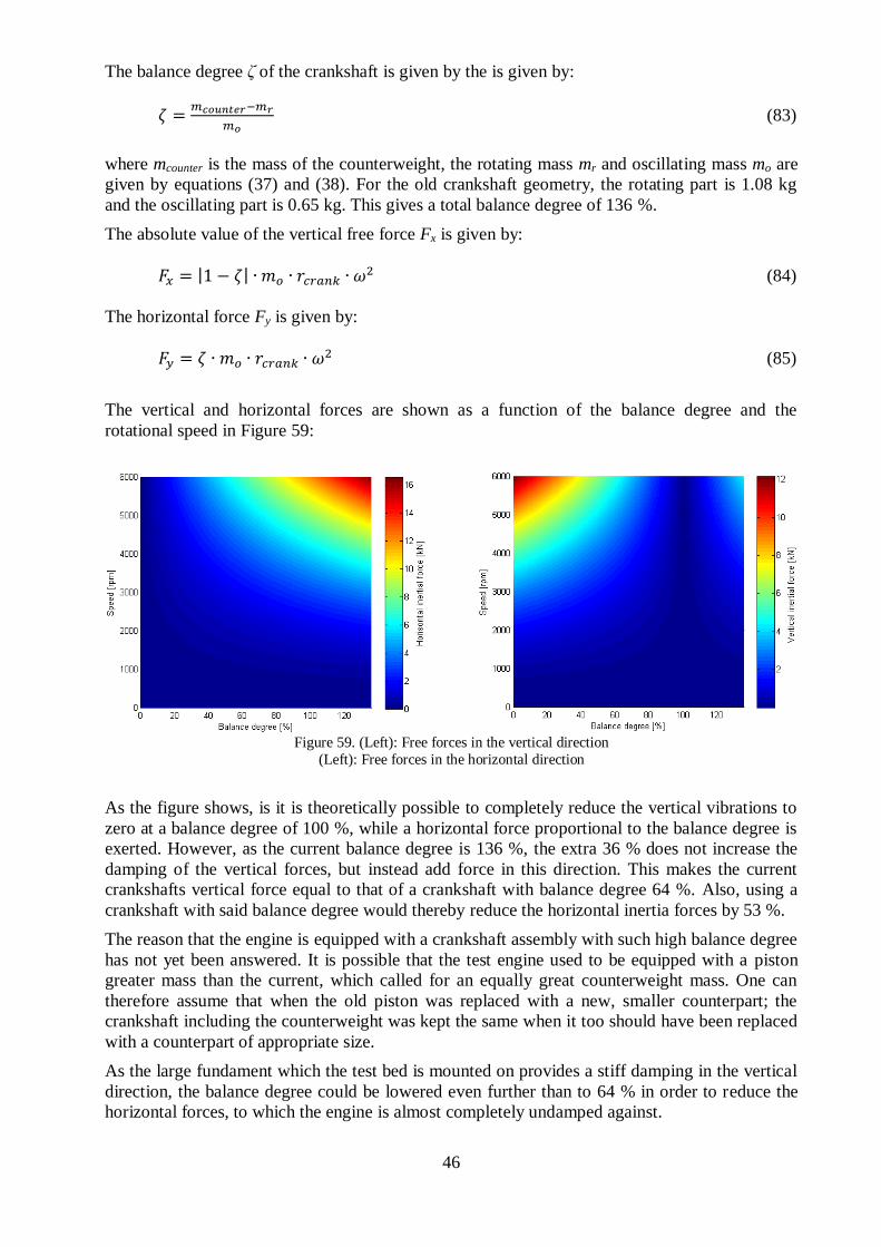
The engine is mounted on a fundament with a large mass, which is more than enough to dampen

and absorb the vertical free forces exerted on the piston. On the other hand, the engine is

completely unsupported in the sideways direction, meaning that the horizontal free forces exerts

a large bending moment around the center which causes large sideways motions at critical

speeds, see Figure 58.

Figure 58. Free forces acting on the engine

46

The balance degree ζ of the crankshaft is given by the is given by:

(83)

where mcounter is the mass of the counterweight, the rotating mass mr and oscillating mass mo are

given by equations (37) and (38). For the old crankshaft geometry, the rotating part is 1.08 kg

and the oscillating part is 0.65 kg. This gives a total balance degree of 136 %.

The absolute value of the vertical free force Fx is given by:

| | (84)

The horizontal force Fy is given by:

(85)

The vertical and horizontal forces are shown as a function of the balance degree and the

rotational speed in Figure 59:

Figure 59. (Left): Free forces in the vertical direction

(Left): Free forces in the horizontal direction

As the figure shows, is it is theoretically possible to completely reduce the vertical vibrations to

zero at a balance degree of 100 %, while a horizontal force proportional to the balance degree is

exerted. However, as the current balance degree is 136 %, the extra 36 % does not increase the

damping of the vertical forces, but instead add force in this direction. This makes the current

crankshafts vertical force equal to that of a crankshaft with balance degree 64 %. Also, using a

crankshaft with said balance degree would thereby reduce the horizontal inertia forces by 53 %.

The reason that the engine is equipped with a crankshaft assembly with such high balance degree

has not yet been answered. It is possible that the test engine used to be equipped with a piston

greater mass than the current, which called for an equally great counterweight mass. One can

therefore assume that when the old piston was replaced with a new, smaller counterpart; the

crankshaft including the counterweight was kept the same when it too should have been replaced

with a counterpart of appropriate size.

As the large fundament which the test bed is mounted on provides a stiff damping in the vertical

direction, the balance degree could be lowered even further than to 64 % in order to reduce the

horizontal forces, to which the engine is almost completely undamped against.

47

At a balance degree of 36%, the maximum horizontal force at 6000 rpm will be lowered by 72.7

%, from 16.5 kN to 4.5 kN. At the same time, the vertical force will only be increased by 3.5 kN;

from 4 kN to 7.5 kN.

Lowering the balance degree to 36 % would mean that the counterweight mass is lowered from

1.97 kg to 1.32 kg.

3.8 Dimensioning the torque sensor

The proper dimensions and properties of the torque sensor are chosen based on the parameters

desired accuracy and range of the measurements.

The primary motivation for using a torque sensor is to allow an accurate continuous

measurement of the engine torque, which may be used to calculate Brake Specific Fuel

Consumption, BSFC continuously.

The BSFC is calculated using:

(86)

where is the fuel flow into the engine, H is the engine power:

(87)

The maximum engine torque is approximated to 2000 Nm, which means that for a BSFC

accuracy with a maximum deviation of 0,002 %, the torque sensor must be a be able to measure

at a maximum deviation of 0.04 Nm.

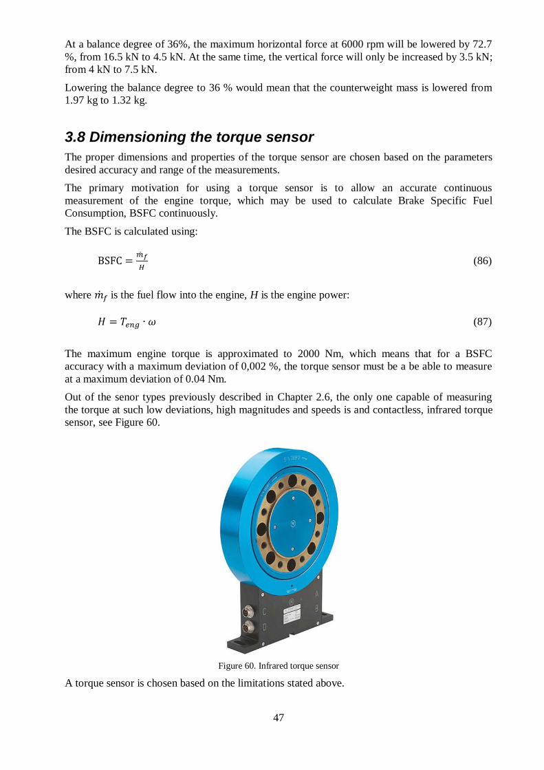
Out of the senor types previously described in Chapter 2.6, the only one capable of measuring

the torque at such low deviations, high magnitudes and speeds is and contactless, infrared torque

sensor, see Figure 60.

Figure 60. Infrared torque sensor

A torque sensor is chosen based on the limitations stated above.

48

49

4 RESULTS

This chapter presents the results achieved by the methods described in the previous chapter

4.1 Overview

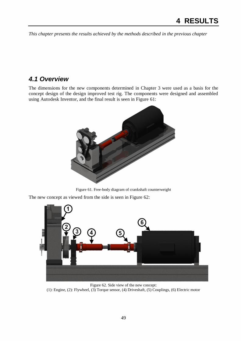
The dimensions for the new components determined in Chapter 3 were used as a basis for the

concept design of the design improved test rig. The components were designed and assembled

using Autodesk Inventor, and the final result is seen in Figure 61:

Figure 61. Free-body diagram of crankshaft counterweight

The new concept as viewed from the side is seen in Figure 62:

Figure 62. Side view of the new concept:

(1): Engine, (2): Flywheel, (3) Torque sensor, (4) Driveshaft, (5) Couplings, (6) Electric motor

50

4.2 Crankshaft

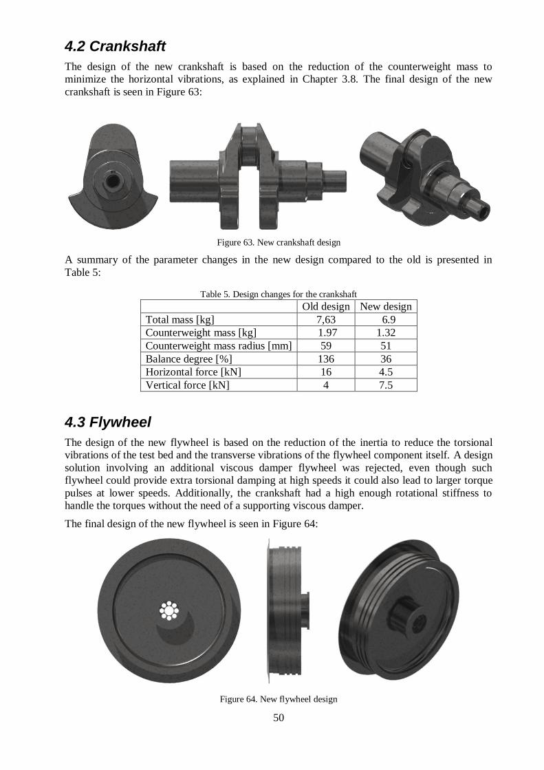
The design of the new crankshaft is based on the reduction of the counterweight mass to

minimize the horizontal vibrations, as explained in Chapter 3.8. The final design of the new

crankshaft is seen in Figure 63:

Figure 63. New crankshaft design

A summary of the parameter changes in the new design compared to the old is presented in

Table 5:

Table 5. Design changes for the crankshaft

Old design New design

Total mass [kg] 7,63 6.9

Counterweight mass [kg] 1.97 1.32

Counterweight mass radius [mm] 59 51

Balance degree [%] 136 36

Horizontal force [kN] 16 4.5

Vertical force [kN] 4 7.5

4.3 Flywheel

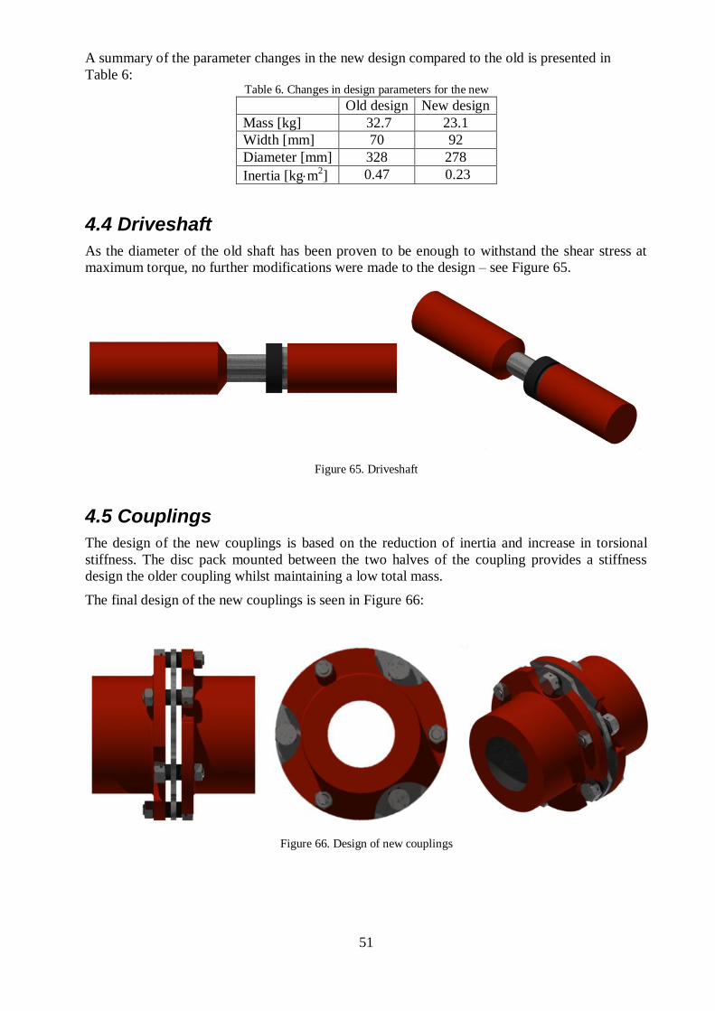
The design of the new flywheel is based on the reduction of the inertia to reduce the torsional

vibrations of the test bed and the transverse vibrations of the flywheel component itself. A design

solution involving an additional viscous damper flywheel was rejected, even though such

flywheel could provide extra torsional damping at high speeds it could also lead to larger torque

pulses at lower speeds. Additionally, the crankshaft had a high enough rotational stiffness to

handle the torques without the need of a supporting viscous damper.

The final design of the new flywheel is seen in Figure 64:

Figure 64. New flywheel design

51

A summary of the parameter changes in the new design compared to the old is presented in

Table 6: Table 6. Changes in design parameters for the new

Old design New design

Mass [kg] 32.7 23.1

Width [mm] 70 92

Diameter [mm] 328 278

Inertia [kgm2] 0.47 0.23

4.4 Driveshaft

As the diameter of the old shaft has been proven to be enough to withstand the shear stress at

maximum torque, no further modifications were made to the design – see Figure 65.

Figure 65. Driveshaft

4.5 Couplings

The design of the new couplings is based on the reduction of inertia and increase in torsional

stiffness. The disc pack mounted between the two halves of the coupling provides a stiffness

design the older coupling whilst maintaining a low total mass.

The final design of the new couplings is seen in Figure 66:

Figure 66. Design of new couplings

52

A summary of the parameter changes in the new design compared to the old is presented in

Table 7:

Table 7. Changes in design parameters for the new couplings

Old design New design

Mass [kg] 15.4 4.5

Width [mm] 69 30

Diameter [mm] 190 128

Stiffness [kNm/rad] 400 450

Inertia [kgm2] 0.139 0.085

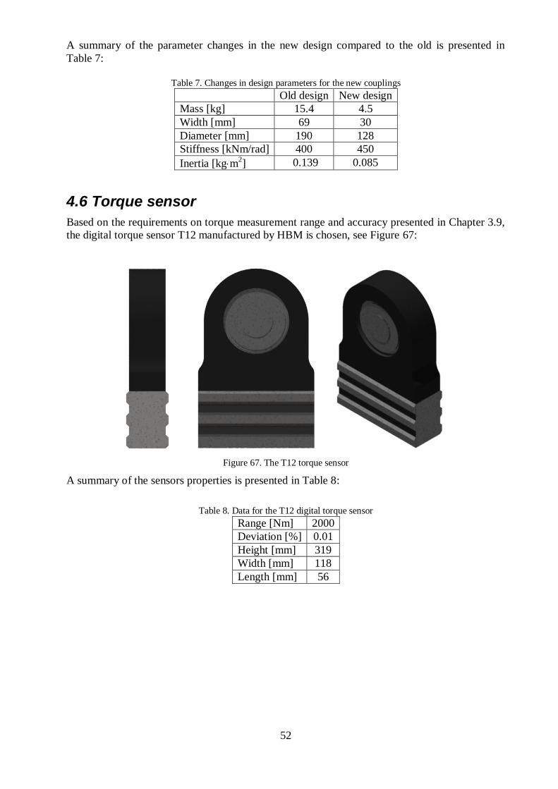
4.6 Torque sensor

Based on the requirements on torque measurement range and accuracy presented in Chapter 3.9,

the digital torque sensor T12 manufactured by HBM is chosen, see Figure 67:

Figure 67. The T12 torque sensor

A summary of the sensors properties is presented in Table 8:

Table 8. Data for the T12 digital torque sensor

Range [Nm] 2000

Deviation [%] 0.01

Height [mm] 319

Width [mm] 118

Length [mm] 56

53

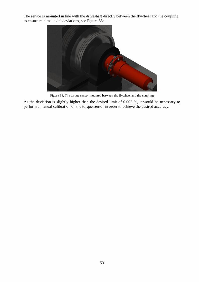
The sensor is mounted in line with the driveshaft directly between the flywheel and the coupling

to ensure minimal axial deviations, see Figure 68:

Figure 68. The torque sensor mounted between the flywheel and the coupling

As the deviation is slightly higher than the desired limit of 0.002 %, it would be necessary to

perform a manual calibration on the torque sensor in order to achieve the desired accuracy.

54

55

5 VERIFICATION

In this chapter the accuracy of the results presented in the previous chapter is verified.

5.1 Verification

In order to verify the results of the transverse frequency analysis, a model of the flywheel is

simulated using ANSYS Modal tool. Vibration modes 1-6 are identified for critical rotation

speed and the corresponding frequencies of the transverse vibrations. The vibration modes are

illustrated in Figure 69, where the large deflections are marked in red and zero deflection is

marked in blue.

Figure 69. The first 6 transverse vibration modes of the flywheel.

The results of the critical speeds and transverse frequencies is summarized in Table 9:

Table 9. Critical transverse frequencies for the flywheel using the ANSYS model

Mode Critical speed [rpm] Transverse frequency [Hz]

1 6640 161

2 6981 224

3 7620 298

4 10800 585

5 15095 1195

6 16703 1280

Comparing the results of the analysis with ANSYS to those using MATLAB, the difference in

critical speed estimation is at most 1.89 %, and the maximum difference in transverse frequency

is at most 4.26 %; which is considered to be an acceptable deviation.

56

57

6 DISCUSSION AND CONCLUSIONS

In this chapter the results presented in the previous chapter is discussed and summarized. The

summary is based on an analysis of results and aims to answer the questions formulated in

chapter 1.

6.1 Discussion

Based on the methods used in Chapter 3 and 5, the results presented in Chapter 4 show that the

new test bed design would be possibly to run at speeds up to 6000 rpm without disruptive

frequencies. However, the methods and models used to obtain the results are based on

simplifications of the physics governing the vibration characteristics of the test rig.

For one, only the vibrations in the engine, driveshaft and electric motor was analyzed in the

study. It is possible that the resonance frequencies of the intake and exhaust manifolds, the

engine and motor mounts, and the rest of the setup could have an influence on the resonance.

Much of the engines combustion characteristics were simplified for the sake of complexity. The

thermodynamic processes were modeled as ideal, and no consideration were taken to more

complex phenomenon such as burn rate, misfire, and cycle-to-cycle variations in pressure which

all affects the engine torque.

The vibration measurements on the test rig were conducted using one accelerometer mounted on

the side of the motor. In order to gain a further understanding of the speed-dependent resonance

frequencies, measurements could have been performed at other parts of the rig as a comparison.

Moreover, a supposed dependency of the engine load on the resonance frequencies was only

analyzed at the lowest and highest load.

Though the methods and results presented in previous chapter were verified and validated using

alternative methods, vibrations and resonances are difficult to model to model fully accurately,

due to the superpositioning of waves and non-linearities of materials. A verification on a

physical adaptation of the design concept would therefore a have been desirable.

The dimensioning of a new electric motor was left out of the analysis, as the acquisition of a new

electric motor was deemed to financially ineffective; even though it is estimated that the

performance of the electric motor should have an influence on the speed-dependent vibrations of

the test bed.

The study has been based on solely damping the test bed vibrations in a passive, mechanical

manner. No consideration was taken into active, controlled damping; which may or may not

have proven more useful for the application.

6.2 Conclusions

The study concludes that:

A design concept for a new single-cylinder engine test bed has been developed.

The new concept shows improved vibrations characteristics and should be possible to run

at the desired max speed of 6000 rpm.

The counterweight of the crankshaft should be lowered to 1.32 kg

The inertia of the flywheel should be lowered to 0.23 kgm2.

The inertia of couplings should be lowered to 0.1 kgm2.

The digital torque sensor T12 of size 2000 is recommended.

58

59

7 RECOMMENDATIONS AND FUTURE WORK

This chapter presents recommendations for more detailed solutions and/or future work.

7.1 Recommendations

In order for further verification of the FE models, it is recommended that further simulations are

conducted using alternate FE programs such as ABAQUS or AVL EXCITE. EXCITE has a

built-in analysis tool specifically designed for the analysis of test bed vibrations, among other

features making it suitable as a tool for further simulations.

In order to improve the accuracy of the engine torque model, simulations in programs such as

GT-Power and AVL Boost is recommendable. These programs are specialized in 1-D

combustion and flow models, which would give further depth to the model accuracy.

Vibration measurements using a larger number of accelerometers mounted at different parts of

the test bed is advisable, as it could verify whether for instance the vibration amplitudes differ

across the test bed.

Measurement on the transverse vibrations of the flywheel could further verify the model

accuracy. These vibrations could be measured using laser mounted perpendicular to the front

side area of the flywheel.

7.2 Future work

Further work is advised in the measurement analysis of the test bed vibrations, in order to

determine what is necessary to measure.

In order to improve the development and testing capabilities of diesel engine, a study on the

dimensioning and design of a single-cylinder diesel engine test bed would be advisable. A test

bed setup with the possibility of testing both spark-ignited engines and diesel engine using a

modular interface for the driveshaft components could also be a the potential subject of a future

study.

A study on active damping of the vibrations may serve as a supplement to the mechanical

damping strategy.

As described in Chapter 4.5, the torque sensor chosen should be calibrated in order to meet the

desired accuracy levels.

A further analysis on the relative accuracy of the test bed measurement equipment is advised.

60

61

8 REFERENCES

[1] Heywood., (2009) “Internal Combustion Engine Fundamentals”,

[2] D. Schrand (2011), “The Basics of Torque Measurement”, Sensor Developments Inc, Orion,

USA

[3] “Bosch Automotive Handbook”, 7th edition, Plochingen, Germany

[4] S. Petersen (1993) “Omkonstruktion av transmissionssystemet mellan en 1-cylindermotor

och en elbroms”, Saab-Scania, Södertälje, Sweden

[5] H. Havtun (2010), “Applied Thermodynamics – Collection of formulas”, Department of

Applied Thermodynamics and Cooling Technology, KTH, Stockholm, Sweden

[6] R. Isermann, J. Schaffnit, S. Sinsel (1999), “Hardware-in-the-loop simulation for the design

and testing of engine-controlsystems”, Technical University of Darmstadt, Germany

[7] W. van Wezel, W.J. Jorna (2009) “Prevention of torsional vibration problems in

reciprocating machinery”, Proceedings of the 38th turbomachinery symposium, Austin, USA

[8] E.J. Nestorides (1958) “A Handbook on Torsional Vibration”, Cambridge University,

Cambridge, Great Britain

[9] E.I. Rivin (1999), “Stiffness and Damping in Mechanical Design”, Wayne State University,

Detroit, USA

[10] L. Vedmar (2006) “Transmissioner”, Lund University, Lund, Sweden

[11] Å. Ekengren (2000), “Mätning av vevaxelns varvtalsvariationer”, KTH, Stockholm,

Sweden

[12] P. Engdahl (2000), ”Mobilt motorförbränningsanalysverktyg”, KTH, Stockholm, Sweden

[13] N. Baddour, J.W. Zu (2000), ”A Revisit of Spinning Disc Models. Part II: Linear Transverse

Vibrations”, Department of Mechanical Engineering and Industrial Engineering, University of

Toronto, Canada

[14] A.J. Mazzei Jr., A. Argento, R.A. Scott (1998), ”Experimental Stability Study of a Two-

Cardan Joint Shaft System”, University of Michigan, USA

[15] L. Råde, B. Westergren (2004), ”Beta – Mathematics Handbook for Science and

Engineering”, Lund, Sweden

62

63

APPENDIX A: TEST BED SPECIFICATION

Engine

Ricardo Hydra MK III. Maximum capacity 110mm x 110mm (Bohr x stroke).

Modular with removable cylinder liners and cylinder heads.

Volume: 550 cm2

Compression ratio: 13.5

Dynamometer

DC brake with pulsed speed stance.

Maximum power 60 kW/81.5 hp

Maximum speed 7000 rpm

Charge Air Cooler

FEV Chargecon. Screw compressor controlling the pressure and temperature of the intake air to

the engine.

Maximum airflow 240 m³/min.

Maximum charge pressure 3.0 bar.

Maximum temperature 150 °C.

Mass flow meter: ABB Sensyflow

DN25 1- 60 kg/h.

DN50,10-400kg/h.

Built-in bypass to run the engine in naturally aspirated conditions with Sensyflow.

Fuel system

Prepared for Petrol, Diesel, E85.

Low Pressure System 0-5 bar,

AVL fuel weight scale.

System for cooling the recirculated fuel in the fuel panel.

High-pressure system 20-320 bar. Limitation today on wires to the motor and accumulators.

Pumping capacity up to 1030 bar.

Cylinder pressure

AVL 670 Indimaster compact

2 channels for cylinder pressure

8 channels of analog signals with crank angle resolution

Emission measurements

Horiba mexa 9100 EGR.

AVL smoke meter 415s.

Data Collection

Rigging sockets for fixed measurement variables

100 pt100 (x100)

15 K-elements (x15)

16 pressure sensors of various types (x16)

4 analog inputs

9 digital inputs

4 analog outputs

4 digital outputs

64

65

APPENDIX B: BESSEL FUNCTIONS

In mathematics, Bessel functions are canonical solutions y(x) of Bessel's differential equation:

( ) (B-1)

where n is an arbitrary real or complex number. [15]

Bessel functions of the first kind:

Bessel functions of the first kind, denoted as Jn(x), are solutions of Bessel's differential equation

that are finite at the origin (x=0) for integer n, and diverge as x approaches zero for negative non-

integer n. It is possible to define the solution by its Taylor series expansion around x =0:

( ) ∑( )

( ) (

)

(B-2)

where Γ is the gamma function, a generalization of the factorial function to non-integer values.

Bessel functions have the characteristics of oscillating sine and cosine functions that decay

proportionally to √ ⁄ , see Figure B-1 for the Bessel functions of the first kind of order n=0, 1,

2:

Figure B-1. Bessel function of the first kind, Jn(x), for integer orders n=0, 1, 2.

Modified Bessel functions of the first kind:

The Bessel functions are valid even for complex arguments x, and an important special case is

that of a purely imaginary argument. In this case, the Bessel equation is rewritten to what is

called the modified Bessel’s equation:

( ) (B-3)

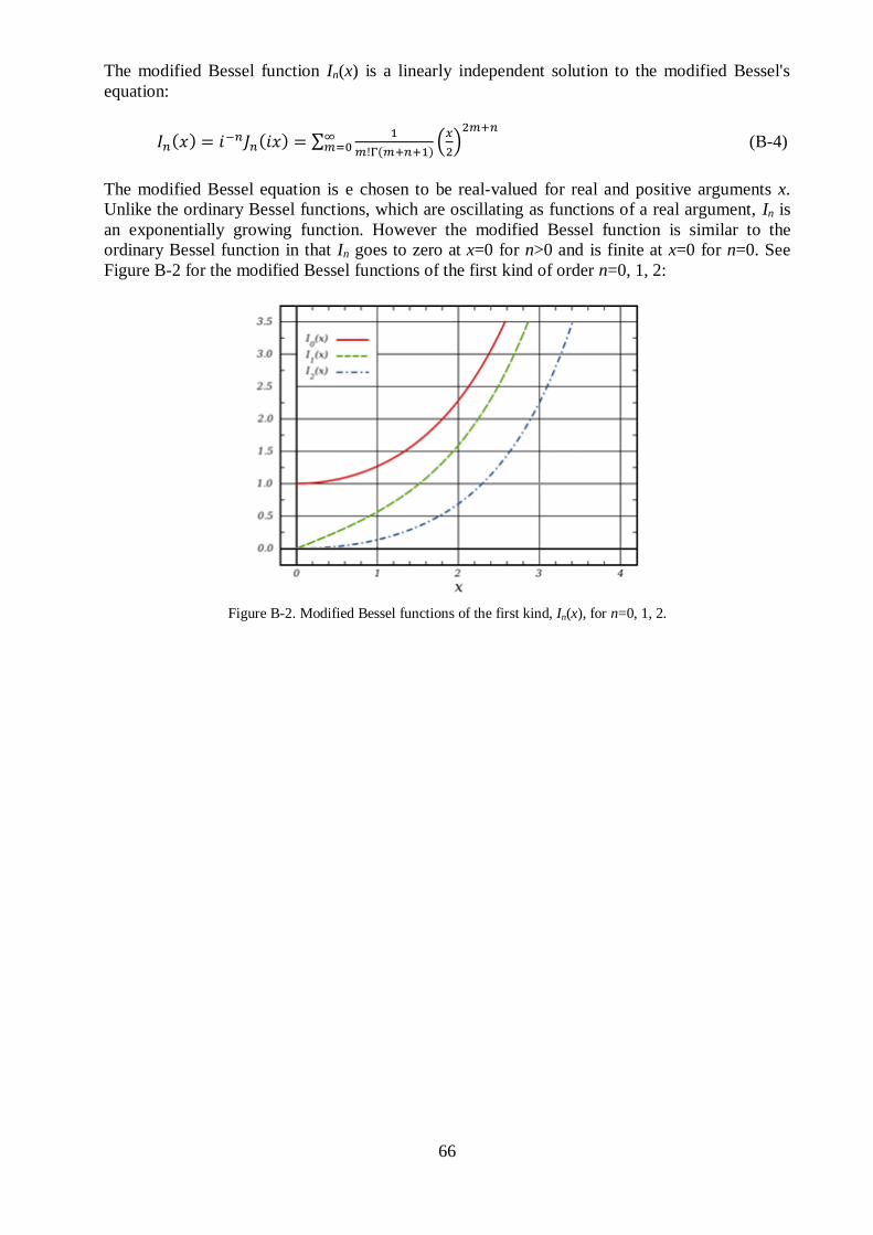
66

The modified Bessel function In(x) is a linearly independent solution to the modified Bessel's

equation:

( ) ( ) ∑

( ) (

)

(B-4)

The modified Bessel equation is e chosen to be real-valued for real and positive arguments x.

Unlike the ordinary Bessel functions, which are oscillating as functions of a real argument, In is

an exponentially growing function. However the modified Bessel function is similar to the

ordinary Bessel function in that In goes to zero at x=0 for n>0 and is finite at x=0 for n=0. See

Figure B-2 for the modified Bessel functions of the first kind of order n=0, 1, 2:

Figure B-2. Modified Bessel functions of the first kind, In(x), for n=0, 1, 2.