daily egg production, spawning biomass and recruitment for...

ABSTRACTThis paper updates estimates of critical stock assess-

ment parameters for the central subpopulation of north-ern anchovy (Engraulis mordax). Ichthyoplankton data from the CalCOFI database were used to implement the historical egg production method and estimate annual mortality curves, from which daily egg production, and egg and larval mortality parameters were derived. Spawning biomass was estimated using historical data under the assumption of a constant daily specific fecun-dity. A Ricker recruitment model, augmented with envi-ronmental factors, was estimated based on historical data and used to predict recruitment using the new spawning biomass data. We found that egg densities were highly variable while larval densities have been persistently low since 1989. Recruitment estimation suggests that poor environmental conditions have potentially contributed to the low productivity. Mortality estimation reveals through an increasing egg mortality rate that low lar-val densities were primarily the result of high mortality during the pre-yolk-sac period.

1 InTRoduCTIonThis paper updates the egg production statistics,

spawning stock biomass, and recruitment time series from 1981–2009 for the central subpopulation of north-ern anchovy (Engraulis mordax) which occupies the Cali-fornia Current Ecosystem from San Francisco, California south to Punta Baja, Baja California, Mexico. It is the largest of the North Pacific subpopulations, and sup-ported a significant U.S. fishery throughout the 1970s and 1980s. In 1978 the fishery came under federal man-agement through the Pacific Fisheries Management Council’s (PFMC) Northern Anchovy Fishery Man-agement Plan (FMP) (PFMC 1978). In 1983 the FMP was amended (Amendment 5) in recognition that harvest should be adjusted annually to reflect the current status of the stock (PFMC 1983) and annual stock assessments were conducted to inform the annual U.S. anchovy har-vest quota.

During the 1980s anchovy abundance started to decline as environmental conditions in the California Current ecosystem became less favorable for anchovy

productivity. Concurrently, the conditions were favor-able for the recovery of the Pacific sardine (Sardinops sagax caerulea) population and fishing effort began to shift from anchovy to sardine. With the shift in fishing effort from anchovy to sardine, conservation and management resources were redirected toward managing the expand-ing sardine fishery, and since 1995 no stock assessments have been conducted for the central subpopulation of northern anchovy (Jacobson et al. 1995). Our updated stock statistics are intended to provide valuable infor-mation about the anchovy’s abundance trajectory over the past 15 years.

The core range of the bulk of the central subpopu-lation lies within the California Bight. Portions of the central subpopulation, thought to be smaller, exist north off the coast of San Francisco and Monterey, as well as south in Mexico (PFMC 2010). The bight has been reg-ularly sampled by research cruises since 1949 and cata-loged in the California Cooperative Oceanogrpahic and Fisheries Investigation (CalCOFI) database. The cruises conducted ichthyoplankton surveys at regular intervals, known as CalCOFI stations (Eber and Hewitt 1979). Anchovy ichthyoplankton from the surveys is preserved and later larvae are counted and lengths recorded, while eggs are only counted. The perserved lengths allow for the binning of larvae counts and aging, known as stag-ing (Lo 1985a).

Numerous methods have been developed to analyze anchovy ichthyoplankton data (Hewitt 1981; Zweifel and Smith 1981; Hewitt and Methot 1982; Lasker 1985). The historical egg production method (HEPM) of Lo (1985a) is the method most amenable to the available CalCOFI data and is the closest to the daily egg pro-duction method (DEPM) (Lasker 1985) currently used for sardine (Lo et al. 2008). The HEPM is a method for estimating daily egg production (P0) and other early life history mortality parameters of archived ichthyoplank-ton data. The HEPM was designed to provide indices of abundance for anchovy dating back to 1951 when no staging data for anchovy eggs were available. The DEPM was designed to estimate the spawning biomass for fish populations with indeterminate fecundity like anchovy and sardine (Hunter and Macewicz 1985) but requires

FISSEL ET AL.: dAILy Egg PRoduCTIon oF noRThERn AnChovyCalCoFI Rep., vol. 52, 2011

116

Daily Egg ProDuction, SPawning BiomaSS anD rEcruitmEnt for thEcEntral SuBPoPulation of northErn anchovy 1981–2009

BENJAMIN E. FISSELNOAA, Alaska Fisheries Science Center

Economics and Social Sciences Research Program 7600 Sand Point Way NE

Seattle, WA 98115 Email: [email protected]

NANCy C. H. LOFisheries Resources Division

Southwest Fisheries Science Center 8604 La Jolla Shores Drive

La Jolla, CA 92037Email: [email protected]

SAMUEL F. HERRICk JR.Fisheries Resources Division

Southwest Fisheries Science Center 8604 La Jolla Shores Drive

La Jolla, CA 92037Email: [email protected]

Fissel r4.indd 116 11/7/11 10:02 AM


117

daily egg production on historical spawning biomass data (Jacobson et al. 1995) thereby assuming constant daily specific fecundity over time. Historical stock and envi-ronmental data was used to estimate the environmental Ricker stock-recruitment model and statistical validity of the model was explored. Bootstrapping was used to characterize variation in mortality.

2 dATA And METhodS

2.1 DataData for the analysis was obtained from the Cal-

COFI database. Data were constrained to the central subpopulation’s core range of the 75 CalCOFI stations (fig. 1) south of CalCOFI line 76.7 and north of line 93.3. Ichthyoplankton surveys over the core range from 1981–2009 were used. Our analysis was constrained to data collected during the peak anchovy spawning season between January and April (Hewitt and Methot 1982; Hewitt and Brewer 1983). We verified in our data that the peak spawning season has remained in this interval. The 75 stations analyzed had a median sampling fre-quency of 2.03 samples per year between Jan–April. Each cruise was weighted equally in our analysis.

Three different types of nets were used for ichthy-

staged eggs. While the more data intensive DEPM is pre-ferred, HEPM provides an unbiased index of the daily egg production (Lo 1985a). The spawning stock bio-mass can then be estimated using daily egg production and daily specific fecundity of the stock (Parker 1980; Hewitt 1985).

The Ricker stock-recruitment model (Ricker 1954) can in turn be used to estimate recruitment from spawn-ing biomass. The stock-recruitment relationships are typ-ically highly variable as it spans the development phases of growth which are subject to a variety of influence. Theories explaining the dynamics of fishes often cite sensitivity in recruitment linked to environmental factors (Aydin 2005) as being a major driver. Previous research shows that anchovy recruitment success is influenced by wind stress driven upwelling (Husby and Nelson 1982; Peterman and Bradford 1987; Rykaczewski and Check-ley 2008) and temperatures in the upper strata of the ocean (Butler 1989; Zweifel et al. 1976; Fiedler et al. 1986). We augment the Ricker model with wind stress and temperature to produce an environmental Ricker stock-recruitment model.

In this paper, daily egg production and mortality parameters were estimated using the HEPM. Spawn-ing biomass was estimated using a model that regressed

Figure 1. CalCOFI Stations in the core range. From: http://www.calcofi.org/cruises/stapos-depth/75stapattern.html accessed 08/23/10

Fissel r4.indd 117 11/7/11 10:02 AM


118

class ages were used to construct larval mortality curves (Lo 1985c). The mortality curve was parameterized such that the fitted DLP at the age of incubation time, t = tI, gives the production at the time of hatching (Ph). Under the assumption that the egg instantaneous mortality rate (IMR) is constant across egg stages3, the egg IMR can be found as the value that is consistent with the observed standing stock of (unstaged) eggs (the dark shaded region in fig. 2). Having obtained the egg IMR over the time of incubation, production of eggs at age 0 (P0), can be estimated using the egg mortality curve from Ph back to the time of spawning.

Residual bootstrapping (Mackinnon 2006) of the annual mortality curves was used to provide annual esti-mates of variability for larval and egg mortality param-eters (appendix B). Bootstrap based variation is reported as 95% confidence intervals (CIs) which were con-structed by taking the 0.025 and 0.975 quantiles of the relevant bootstrapped distribution. Details on the boot-strap procedure are provided in appendix B.

2.2.1 Mortality curves and daily egg production. An annual Pareto type mortality curve was used to model the mortality of larvae from the time of hatching. The variables of daily larval production, dlpc,s, average age of larvae (tc,s) and incubation time tI

s for larval class c in year s (see appendix A) are used to identify the parameters

oplankton surveys over 1981–2009. The CalBOBL or Bongo net (CB), the CalVET (CVT ) and two con-nected CalVET nets called the PairOVET (PV ) (CVT and PV are referred to collectively as CVT/PV )1. Our analysis utilizes ichthyoplankton samples from CB and CVT nets for 1981–1984 and CB and PV nets for 1985–2009.

2.2 Daily egg productionEgg production methods estimate the production of

eggs at age zero, the time of spawning. Estimation of age-zero egg production per 10 m2 (P0) from the counts of eggs and larvae was carried out in a series of steps. Pro-cedures for correcting raw ichthyoplankton counts and aging have followed the literature closely and incorpo-rate previously derived parameters. Appendix A provides details on the methods used for egg and larval density construction and aging, and they are summarized in the following paragraph.

First, larvae were sorted into size classes based on pre-served larval size. The size classes were 2.5 mm, 3.25 mm, 4.25 mm,…, 9.25 mm2. Extrusion and avoidance correc-tions were applied and standard haul factors were used to rescale egg and larval counts to a 10 m2 area-density (appendix A1). The time it takes eggs to reach the devel-oped stage, incubation time (tI), was calculated using a temperature-dependent relationship (Lo 1983). A live larval length correction was made to preserved samples, and live lengths were used in a temperature and month-dependent two-stage Gompertz growth curve (GGC) (Lo 1983; Hewitt and Methot 1980) to estimate larval age (t) (appendix A2). The first stage of the GGC spans the first three larval classes (2.5 mm, 3.25 mm, 4.25 mm) and is designed to model growth over the period of yolk-sac consumption. The second stage of the GGC covers post-yolk-sac consumption growth (5.25 mm,…, 9.25 mm) when larvae must seek out food in their envi-ronment. Aggregation of the samples over cruises and stations yielded annual age and density statistics for the region. The daily larval production (DLP) is the daily production of larvae in a size class per 10 m2 areadensity, and was constructed as the standing stock of larvae in a size class over the number of days that larvae spend in that size class as determined by the growth curve.

Methods for the estimation of the mortality curves are presented in the following subsection 2.2.1. However, it is useful to first summarize the approach. Figure 2 dis-plays a conceptual graph of the HEPM estimation pro-cess. First, daily larval production and corresponding size

(Labels indicate larval classes)Age (t)

eggs 2.5

3.75

4.75

5.75

6.75

7.75

8.75

9.75

Log

daily

pro

duct

ion

Conceptual graph of mortality estimation

�

�

�

�

�

�

�

�

log(Ph)

log(eggs)

Egg mortality line

tI

log(P0)

00

� Log daily larval productionLog larval mortality curve

Figure 2. Conceptual graph of HEP mortality estimation, on log-linear axes.

1Further details on sampling procedures and nets are available from the South-west Fisheries Science Center (SWFSC), CalCOFI, Smith and Richardson (1977). 2Larval class sizes greater than 9.25 mm were discarded because mature larvae are more adept at avoiding nets thereby introducing significant bias into production calculations (appendix A3). 3This assumption was verified in Lo (1985a) for select years.

Fissel r4.indd 118 11/7/11 10:02 AM


119

the SSBs is proportional to P0,s. With this assumption a simple linear regression without a constant is estimated:

SSBs = γ P0,s105Λ + ηD1s + ϵs (4)

where P0,s105 is the daily egg production per km2 Λ is the area of the core CalCOFI region (approx. 200,500 km2). From 1981–1986 data from south of the Mexi-can border was used by National Marine Fisheries Service's Southwest Fisheries Science Center (SWFSC) to calculate SSBs and other stock statistics, D1 is a categorical vari-able accounting for this: 1981–1986 (D1=1) and 1987-2009 (D1=0). The model was fit using the estimated P̂0,s (equation 3) and SSBs from Jacobson et al. (1995)

over the years 1981–1995. The fitted model was used to estimate the SSBs from 1981–2009. The standard esti-mate of prediction error associated with ordinary least squares is reported.

2.4 RecruitmentEstimates of spawning stock biomass were used in

conjunction with a Ricker curve to provide recruit-ment estimates and explore the impact of environmental conditions. The last anchovy stock assessment (Jacobson et al. 1995) provided estimates of both spawning stock biomass and recruitment for the years 1964–1995. Con-sistent with Jacobson et al. (1995) we refer to recruits as age-0 anchovy on July 1.

Two environmental factors were incorporated into our recruitment model, north-south (N-S) wind stress and sea surface temperature5. The Ricker stock- recruitment model was augmented with these vari-ables in the exponential, which yields an environmental Ricker model:

Rs = A*SSBs * eB *SSBs+ρ1*NSWind5s+ρ2*tanoms + εs (5)

where Rs is recruitment in year s, tanoms is the mean annual sea surface temperature (SST) anomay at Scripps pier and NSWind5s is the 5% quantile of the annual north-south wind stress anomaly distribution. Wind stress and sea surface temperature anomalies were com-puted as deviations from the monthly means across all available years. Recruitment and spawning biomass were normalized by their standard deviation, then fit using NLS over the stock and environmental data from 1964–1995. The standard Ricker curve (ρ1 = ρ2 = 0) was used as the null model, M 0, to evaluate the benefit of added

in the model. Each year was estimated independently using the equation:

dlpc,s = Ph,s (tc,s ∕ t Is )

– βs + εc,s (1)

where the mortality curve parameterization was chosen by Lo (1985a) so that Ph,s is the production at the time of hatching (t = t I

s), and βs is the coefficient of the lar-val instantaneous mortality rate. The larval instantaneous mortality rate decreases as larvae age, and at age t is β/t (Hewitt and Brewer 1983). We assume the error term, εc,s, is distributed with a mean-zero, however, we allow for heteroskedasticity across ages through our bootstrap methods (appendix B). Equation 1 was fit using nonlin-ear least squares (NLS). A grid search over initial condi-tions was performed and the parameters that minimized the sum-of-squared errors were used. A residual boot-strap of equation 1 was used to construct 95% CIs for βs and Ph,s (appendix B).

An exponential curve, which applied a constant instantaneous mortality rate (IMR), α, was used to model egg mortality to Ph,s: log(P0) – α*t = log(egg production at age t), for t∈(0,t I ), where log(P0) – α*t I = log(Ph)4. Manipulation of the definition for the observed standing stock of eggs and the production at the time of hatching (Lo 1985a) yields a definition that was used to calculate the egg IMR:

ms eαs*tIs – 1 = (2) Ph,s αs

where ms is the observed corrected standing stock of eggs, and the egg IMR, αs, was estimated by iterative method. Daily egg production can now be estimated as the production at time zero, P0,s, necessary to produce the estimated Ph,s give the egg mortality rate αs, and the time it takes to incubate t I:

P0,s = Ph,s eαs*tIs (3) Ninety-five percent CIs for αt and P0,s were derived

by re-estimating equations 2 and 3 at each iteration of the larval bootstrap (appendix B).

2.3 Spawning stock biomass estimation To obtain estimates of SSB overlapping, historical data

from Jacobson et al. (1995) was used and daily specific fecundity, Ds, was assumed constant over time so that

4Lo (1985a) provided two separate mortality estimates: first under the assump-tion of constant IMR to yolk-sac larval stage, and second constant through the first yolk-sac larval stage. Constant mortality through the first larval stage was a helpful assumption for the historical data used because CVT/PV samples were not present. The use of the CVT/PV nets in our data gives us sufficiently ac-curate sampling from from smaller larvae classes.

5North-south (N-S) wind stress data were obtained from the Environmental Research Division of the SWFSC through their Live Access Server http://www.pfeg.noaa.gov/products/las.html. The wind stress vectors are National Center for Environmental Predictions derived monthly wind stresses from the location 32.5 degrees north and 117.5 degrees west, and span 1948–2009. Data on Scripps pier SST data were obtained from the ocean informatics datazoo http://oceaninformatics.ucsd.edu/datazoo/data/ hosted by Scripps Institution of Oceanography.

Fissel r4.indd 119 11/7/11 10:02 AM


120

had a range of 6.3/10 m2 to 648.8/10 m2 and a mean of 166.3/10 m2 with pronounced episodes of high den-sity particularly in 2005–2006 (table 1). Larvae densities do not track the dynamics of egg densities closely and are considerably smaller than densities observed through the mid to late 1980s; similar to patterns in 1951–1982 (Lo 1985a).

Egg density closely mirrors P0 (figs. 3 and 4, table 1). P0 displays high post-1989 production around 1997, 2001 and a pronounced episode of high density in 2005. In the early ’80s DEP appears comparatively low in con-trast to the relative egg density owing to the low egg IMR (α) during that period (fig. 4 upper-right panel, table 1). The larval mortality coefficient (β) has been variable but has maintained an average value of approx-imately –1.89 (fig. 4 lower right panel). In contrast, the egg IMR has been increasing from low levels in the early ’80s to over 2 in the late 2000s. A linear time trend has been superimposed on the egg IMR time series and shows that the egg IMR has been increasing by approxi-mately 0.06 per year. Bootstrap CIs indicate that estima-tion of the egg IMR is more precise than the coefficient of larval mortality (fig. 4 right panel). The imprecision in the estimation of β is largely due to higher residual variance in the pre-yolk-sac-consumption larval phases (fig. B1). CIs for DEP indicate that the random varia-tion in larval mortality does not significantly contribute to the observed pattern of DEP.

The spawning stock has shown periods of low bio-mass since 1989, but has been highly variable (fig. 5, table 2) with high post-1990 biomass around 1997, 2001

information from the full environmental Ricker model, MWT (ρ1, ρ2 unconstrained). The Akaike information cri-terion (AIC) was used to compare the models. The ratio of likelihoods was formed as L(M0)/L(MWT) = exp((AICWT – AIC0)/2), which is the likelihood that the constrained null model minimizes the information loss relative to the unconstrained model that uses the environmental fac-tors (Burnham, k. P. and D. R. Anderson (2002)), which we denote by I(MWT) ≤ I(M0). Similar AIC probability calculations were carried out on different model speci-fication to assess the relative contribution of the individ-ual environmental factors. SSB estimates obtained from equation 4 were used with the fitted environmental Ricker model to estimate recruitment from 1981–2009.

3 RESuLTS Annual density plots for the core CalCOFI stations

show the temporal variation of eggs and larvae (fig. 3, table 1). Since approximately 1989, egg densities in general, have been lower although more highly vari-able than the years preceding. Prior to 1989 densities ranged from 2182/10 m2 to 7063/10 m2 with a mean of 4276/10 m2, while later densities showed a range of 508/10 m2 to 11091/10 m2 and a mean of 2070/10 m2 with pronounced episodes of high density particularly in 2005–2006 (table 1). In contrast, larvae densities have declined fairly steadily since 1989 except for 2005 when an increase in larval density was associated with the cor-respondingly high egg density (fig. 3 right panel). Lar-val densities ranged from 394.1/10 m2 to 2870.2/10 m2 with a mean of 1177.9/10 m2 prior to 1989, and after

1981 1984 1987 1990 1993 1996 1999 2002 2005 2008

Northern anchovy egg densities 1981−2009

year

020

0040

0060

0080

0010

000

Eggs

/10m

2

1981 1984 1987 1990 1993 1996 1999 2002 2005 2008

Northern anchovy larval densities 1981−2009

year0

500

1000

1500

2000

2500

Larv

ae/1

0m2

Figure 3. Annual egg and larval densities per 10 m2 in the core CalCOFI region 1981–2009.

Fissel r4.indd 120 11/7/11 10:02 AM


121

discrepancy but the respective trends are nearly identi-cal (R2 = 0.825) (table 3). The high biomass in 2005 is not without precedent; similar levels were seen around 1976. The parameter on SSB, γ, was significant at the

and a pronounced episode of high biomass in 2005–2006. SSB has been comparatively lower in recent years. For the overlapping years of Jacobson et al. (1995) SSB, and our SSB estimates (fig. 5 left panel) there is some

TABLE 1Annual egg, larval and mortality statistics

Year Egg dens. 10 m2 Larvae dens. 10 m2 β Ph α P0

1981 2685.26 1673.18 –1.96 1015.49 –0.04 912.35 [–2.05,–1.84] [866.5,987.3] [–0.05,0.04] [862,983]1982 2896.23 693.44 –1.56 255.62 0.7 2279.5 [–1.74,–1.23] [186.4,280.1] [0.61,0.8] [2052,2495]1983 2181.7 928.23 –2.02 616.87 0.24 1139.14 [–2.17,–1.85] [504.4,616.2] [0.2,0.34] [1061,1242]1984 3869.8 1189.92 –1.82 598.47 0.56 2770.29 [–1.92,–1.68] [497,572.3] [0.52,0.6] [2601,2826]1985 3853.01 394.07 –2.67 263.97 0.76 3177.28 [–2.93,–2.06] [191,282.3] [0.71,0.88] [3022,3578]1986 7063.25 1144.54 –2.54 1196.2 0.43 4239.8 [–2.69,–2.41] [1129.7,1322.1] [0.38,0.47] [3993,4434]1987 5595.11 2870.22 –2.2 1719.78 0.05 2021.12 [–2.24,–2.15] [1647.7,1714.2] [0.05,0.08] [1994,2069]1988 6060.64 529.37 –2.22 282.93 0.82 5254.26 [–2.48,–1.85] [234.7,346] [0.77,0.93] [5011,5846]1989 745.66 155.23 –2.06 80.66 0.62 542.7 [–2.46,–1.2] [43,87] [0.5,0.82] [464,656]1990 1862.97 534.85 –1.96 313.13 0.5 1239.04 [–2.18,–1.69] [191.5,255.6] [0.47,0.61] [1133,1336]1991 1634.47 421.06 –1.28 114.16 0.94 1658.65 [–1.47,–0.91] [80.1,129.2] [0.82,1.05] [1467,1791]1992 1095.67 167.43 –1.89 85.94 0.98 1165.09 [–2.35,–1.28] [54.9,105.3] [0.83,1.16] [1011,1331]1993 507.68 108.98 –1.52 37.55 0.87 476.87 [–2.01,–0.68] [18.7,56.5] [0.68,1.23] [403,642]1994 932.9 271.69 –2.15 125.74 0.52 609.87 [–2.5,–1.83] [123.2,165.1] [0.44,0.6] [571,684]1995 1857.66 99.84 –2.1 33.36 1.2 2270.21 [–2.63,–1.26] [28.8,59.5] [1.24,1.56] [2370,2927]1996 2041.04 259.41 –2.65 156.04 0.86 1912.72 [–2.93,–2.1] [142.5,201.6] [0.8,0.98] [1836,2151]1997 3753.55 130.25 –1.41 39.92 1.82 6884.84 [–1.88,–0.83] [22.8,56.1] [1.57,1.94] [5952,7319]1998 572.02 85.71 –1.73 36.36 1.23 740.98 [–2.08,–1.07] [22.3,39.3] [1.09,1.39] [662,816]1999 795.65 140.46 –1.97 71.66 0.64 581.51 [–2.33,–1.5] [45.3,77.2] [0.53,0.75] [499,646]2000 1106.24 93.36 –2.47 55.3 1.06 1226.33 [–2.85,–1.6] [28.9,56.2] [0.97,1.26] [1127,1420]2001 2722.55 101.16 –2.49 63.22 1.33 3689.34 [–2.86,–1.65] [31,57.7] [1.22,1.46] [3391,4010]2002 823.98 49.78 –0.9 7.39 1.45 1200.32 [–1.57,–0.28] [4,14.3] [1.24,1.7] [1038,1401]2003 862.19 70.08 –1.58 21.63 1.31 1150.54 [–1.93,–1.05] [14.3,27.5] [1.22,1.5] [1078,1307]2004 1693.4 55.18 –2.61 33.95 1.51 2592.44 [–2.99,–1.7] [15.9,40] [1.32,1.7] [2274,2892]2005 11091.12 648.81 –1.27 143.84 1.53 17161.25 [–1.39,–1.12] [137.3,171.6] [1.57,1.67] [17617,18637]2006 6394.01 57.13 –1 9.41 2.34 14972.47 [–1.8,0] [3.5,26.3] [1.99,2.73] [12610,17272]2007 1142.23 19.76 –1.13 3.41 2.03 2320.7 [–1.87,–0.36] [1.7,5.8] [1.77,2.21] [2023,2524]2008 808.21 6.3 –1.92 1.89 2.02 1633.54 [–2.46,–0.13] [0.6,2.5] [1.79,2.27] [1447,1836]2009 1044.16 14.8 –1.6 3.42 1.92 2012.21 [–1.9,–0.32] [2,4.5] [1.86,2.15] [1945,2249]

Egg and larval densities, the coefficient of the larval instantaneous mortality rate (IMR) (β), larval production at the time of hatching (Ph), egg IMR (α), and egg production at age at age zero per 10 m2 (P0). 95% bootstrap larval mortality confidence intervals are in brackets below the estimates.

Fissel r4.indd 121 11/7/11 10:02 AM


122

ton of SSB6. However, because of the assumptions and the reduced form nature of the regression γ may be capturing some latent changes over time. The implied daily specific fecundity (number of eggs produced per day per unit fish weight) per metric ton of biomass was 1/γ = 2.532 E+08. Aggregate specific fecundity can be obtained by multiplying this by the SSB.

0.1% level (table 3) and can be roughly interpreted as the inverse of the daily specific fecundity per metric

1981 1984 1987 1990 1993 1996 1999 2002 2005 2008

Northern anchovy daily egg production 1981−2009

year

050

0010

000

1500

0P 0

/10m

2

1980 1985 1990 1995 2000 2005 2010

0.0

0.5

1.0

1.5

2.0

2.5

year

IMR

α̂ = 0.17 + 0.062(year − 1981)

1980 1985 1990 1995 2000 2005 2010−3.5

−2.5

−1.5

−0.5

year

IMR

β = − 1.886

Figure 4. Annual daily egg production (P0) (left panel) and egg IMR and coefficient of larval IMR (right panel). IMR regression coefficients displayed have a p-value ≤ 0.01. Error bars represent 95% bootstrapped larval mortality confidence intervals.

1964 1968 1972 1976 1980 1984 1988 1992 1996 2000 2004 2008

Fissel et al. 2011Jacobson et.al. 1995

Spawning Stock Biomass 1964−2009

year

Biom

ass

mt

020

0000

4000

0060

0000

8000

0010

0000

012

0000

0

1981 1984 1987 1990 1993 1996 1999 2002 2005 2008

Spawning Biomass 1981−2009

year

Biom

ass

mt

050

0000

1000

000

1500

000

Figure 5. Comparison of historical and new annual spawning stock biomass (SSBs) 1964–2009 (left panel). Annual spawning stock biomass 1981–2009 (right panel).

6The fecundity parameters of the stock relate SSB to P0 (Parker 1980; Hewitt 1985). The stocks sex-ratio (Q), the proportion of mature females spawning (F), and the average batch fecundity (E) relative to the mature female weight (W) give the daily specific fecundity, 1/γ = Q*F*(E/W). The daily specific fecundity and daily egg production can be related to the spawning biomass by: P0 = SSB*(1/γ).

Fissel r4.indd 122 11/7/11 10:02 AM


123

TABLE 2Annual spawning biomass and recruitment statistics

Year Spawning biomass SSB Predic. Error Recruitment Wind S. .05 quant Temp. mean

1981 411825.77 76469.05 670506.17 –0.848 0.5121982 520106.22 68050.61 2292236.85 –1.728 0.0221983 429787.65 74202.51 557112.61 –0.850 0.8551984 558977.70 68459.06 1058457.90 –1.633 1.1991985 591212.10 70215.62 482741.42 –0.320 0.1091986 675365.57 80059.39 282065.59 –0.115 0.6121987 160075.84 46971.72 393716.32 –0.732 0.4511988 416146.22 122111.51 851826.18 –0.739 –0.1131989 42983.16 12612.73 193872.87 –0.886 0.0811990 98134.15 28795.91 240347.47 –0.790 0.7861991 131368.04 38547.87 331156.59 –0.384 –0.1441992 92276.93 27077.20 102489.76 –0.221 1.1371993 37769.26 11082.79 38983.16 –0.056 1.1491994 48302.66 14173.65 56698.02 –0.070 0.9101995 179804.42 52760.76 594143.98 –1.170 0.6811996 151490.66 44452.53 261865.36 –0.600 0.8581997 545291.08 160007.02 352430.96 –1.067 2.0841998 58686.52 17220.63 71883.07 –0.218 1.0771999 46056.91 13514.67 311754.70 –0.906 –0.6092000 97127.44 28500.51 154578.31 –0.273 0.5822001 292202.02 85742.05 389139.87 –0.308 0.2762002 95067.77 27896.13 224820.84 –0.487 0.2902003 91125.05 26739.20 180510.05 –0.443 0.5362004 205325.91 60249.63 195895.29 –0.344 1.2372005 1359200.63 398835.88 117862.60 –0.214 1.1662006 1185845.47 347967.55 190403.04 –0.378 0.9962007 183803.71 53934.28 212452.88 –0.132 0.5762008 129379.08 37964.24 175467.13 –0.100 0.4272009 159370.30 46764.69 590413.16 –0.965 0.167

Spawning biomass (SSB) (mt) with prediction error and recruitment (mt). Mean sea surface temperature anomaly (Temp.) and the 0.05 quantile of the north-south wind stress anomaly distribution (Wind S.).

TABLE 3Spawning Stock Biomass Regression

Coefficients Estimate Std. Error t value Pr(>|t|)

γ 3.950E-09 1.159E-09 3.408 0.00467** η 3.396E+05 8.822E+04 3.849 0.00201**

Signif. codes: 0 '***' 0.001 '**' 0.01 '*' 0.05 '.' 0.1 ' ' >0.1 Residual standard error: 166500 on 13 deg. of freedomMultiple R2: 0.848, Adjusted R2: 0.825F-statistic: 36.34 on 2 and 13 DF, p-value: 4.749E-06

Coefficients of the regression are the inverse of the daily specific fecundity per metric ton of SSB (γ) and a categorical variable for the inclusion of Mexican data, 1981–1986 (η).

TABLE 4Standard and environmental Ricker regressions

Standard Ricker M0 Environmental Ricker MWT

Coefficient Estimate Std. Error Coefficient Estimate Std.Error

A 1.3991* 0.5437 A 0.5659 0.2959 B –0.5074* 0.1384 B –0.5074** 0.1384 ρ1 –106.171** 36.359 ρ2 –0.5663* 0.2145

Resid std. error: 0.9815 Resid std error: 0.8026 df = 3; AIC = 93.5538 df = 5; AIC = 82.4666

Signif. codes: 0 '***' 0.001 '**' 0.01 '*' 0.05 '.' 0.1 ' ' >0.1

Comparison of the standard and environmental Ricker recruitment models with coefficient estimates for Ricker model parameters, the 0.05 quantile of the N-S wind stress anomaly (ρ1) and mean sea surface temperature anomaly (ρ2).

Fissel r4.indd 123 11/7/11 10:02 AM


124

0 200000 400000 600000 800000 1000000 1200000 1400000

0e+0

01e

+06

2e+0

63e

+06

4e+0

6

Fitted values from the environmental Ricker curve 1964−1995

SSB mt

Rec

ruitm

ent m

t

19641965

1966

19671968

1969

1970

1971

1972

1973

1974

1975

1976

1977

1978

1979

1980

1981

1982

1983

1984

1985

19861987

1988

1989 19901991

19921993

1994

1995

1964

1965

19661967

19681969

1970

1971

1972

1973

19741975

19761977

1978

1979

1980

1981

1982

1983

1984

1985

1986

19871988

19891990

1991

199219931994

1995

Fitted valuesJacobson et al. 1995Standard Ricker

0 200000 400000 600000 800000 1000000 1200000 1400000

050

0000

1000

000

1500

000

2000

000

Stock−recruitment estimates 1981−2009

SSB mt

Rec

ruitm

ent m

t

1981

1982

1983

1984

1985

1986

1987

1988

19891990

1991

199219931994

1995

19961997

1998

1999

2000

2001

20022003 2004

2005200620072008

2009

Fissel et al. 2011Standard Ricker

Figure 6. Fitted values of environmental Ricker model 1964–1995 (left panel) and predicted recruitment from the environmental Ricker curve 1981–2009 based on our ^SSBs (right panel).

Fissel r4.indd 124 11/7/11 10:02 AM


125

1964 1968 1972 1976 1980 1984 1988 1992 1996 2000 2004 2008

Fissel et al. 2011Jacobson et.al. 1995

Recruitment 1964−2009

year

Biom

ass

mt

0e+0

01e

+06

2e+0

63e

+06

4e+0

6

1981 1984 1987 1990 1993 1996 1999 2002 2005 2008

Recruitment 1981−2009

year

Biom

ass

mt

050

0000

1000

000

1500

000

2000

000

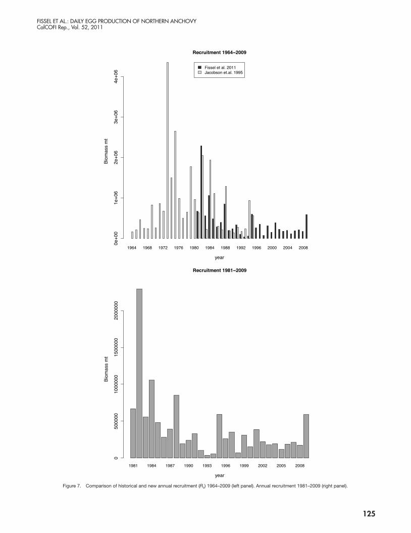
Figure 7. Comparison of historical and new annual recruitment (Rs) 1964–2009 (left panel). Annual recruitment 1981–2009 (right panel).

Fissel r4.indd 125 11/7/11 10:02 AM


126

without precedent and were observed in the mid to late ’60s (fig. 7 left panel).

4 dISCuSSIonThe anchovy ichthyoplankton data are not without

their shortcomings. Previous anchovy assessments (Jacob-son et al. 1995) used the CB, CVT and PV surveys with targeted adult and juvenile trawl surveys, and aerial spot-ter plane data. The latter two surveys are no longer con-ducted, hindering the calculation of a time-varying daily specific fecundity. Previous assessments also had staged eggs allowing the implementation of the DEPM and fundamental growth parameters had been recently esti-mated. While the precision of available parameters (Lo 1983) should be sufficiently accurate for HEPM estima-tion, parameters could hypothetically be time-varying and require updating to reflect the current environmen-tal regime. Updated and extended sampling and research could provide further accuracy in future studies, but would not affect the trend in our estimates as these are driven by observed egg and larval densities.

The episodes of high egg densities, SSB and P0 around 1997 and particularly in 2005 are prominent fea-tures of the data (fig. 3). Despite the periodic surges in spawning productivity we observed comparatively low larval densities (fig. 3). The low larval counts result in low corresponding estimates of the production at the time of hatching (Ph) which by the estimation proce-dure then translates into a high egg IMR. However, Ph is not directly observed and is estimated. Thus, the hatching transition itself has the potential to be a source of mortality, and one potentially susceptible to a vari-ety of influences. Mortality at, or very shortly after, the time of hatching could confound egg IMR estimates. Regression discontinuity could be used to test this but would require staged eggs and thorough sampling to ensure accurate densities estimates around the hatch-ing threshold.

Interpreted within the context of the modeling approach, the steady increase in the egg IMR is the primary cause of the low larval densities as opposed to the comparatively more stable coefficient of larval mortality (fig. 4). High mortality during the larval post-

The environmental factors were significant in the Ricker stock-recruitment model (fig. 6, table 4). The .05 quantile of the north-south wind stress anomaly was sig-nificant at the 0.1% level, and mean sea surface temper-ature anomaly at the 1% level. The contribution of the variables to explaining recruitment was further explored through an analysis of the AIC statisitics from different models (table 5). The unconstrained model MWT had the lowest AIC. Models with only temperature (MT) and only wind stress (MW) were compared to the null model (M0), the standard Ricker curve (section 2.4). The likelihood ratio statistic shows the contribution of the incorporating environmental information (table 5). The information gain in predicting recruitment provided by both environmental factors relative to the null model I(MWT) ≤ I(M0) is 0.004, below a 1% significance thresh-old. Temperature alone provides some improvement relative to the null model I(MT) ≤ I(M0) with a likeli-hood statistic of 0.08 which is below a 10% significance threshold, while a model with only wind stress I(MT) ≤ I(M0) is marginally above a 5% significance threshold with statistic of 0.05. The full model was compared to the model with only wind stress I(MWT) ≤ I(Mw) and had a likelihood ratio statistic of 0.08 which is below a 10% level of significance. Both wind stress and temper-ature are significant in explaining recruitment, however wind stress has a comparatively larger influence. Both environmental variables were used in reported recruit-ment estimation (table 2). Graphical comparison of the standard Ricker and the environmental Ricker (fig. 6 left panel) shows that the temperture and wind stress produce improved fits for many years (e.g. 1975, 1977, 1982, and others), although this is not uniformly true for all years (e.g. 1976, 1980, and others).

The difference between the recruitment estimates and the standard Ricker curve shows the estimated influence of the environmental factors for 1981–2009 (fig. 6 right panel). Recruitment estimates above the standard Ricker line indicate favorable environmental conditions, while estimates below indicate the opposite. Many recent years, even when spawning biomass is high, fall below the stan-dard Ricker curve. Comparison of Jacobson’s historical data to ours show that the low recruitment levels are not

TABLE 5AIC comparisons of the Ricker model specifications

AIC statistics

Model M 0 (ρ1 = ρ2 = 0) MT (ρ1 = 0, ρ2uc) MW (ρ1uc,ρ2 = 0) MWT (ρ1uc,ρ2uc) AIC 93.5538 88.5827 87.5796 82.4666

Relative information likelihood statistics

Model Comp. I(MWT) ≤ I(M 0) I(MT) ≤ I(M 0) I(MW) ≤ I(M 0) I(MWT) ≤ I(Mw) Likelihood 0.0039 0.0833 0.0504 0.0776

Model M 0 is the standard Ricker null model, MWT is the full environmental Ricker model, and MW and MT are models with only wind and temperature respectively. Likelihood ratios show relative information (I (*)) content. (uc means the coefficient was unconstrained).

Fissel r4.indd 126 11/7/11 10:02 AM


127

tify the point during the development process that these factors (or factors for which they’re proxying) are influ-encing mortality. Nonetheless, one can interpret envi-ronmental Ricker as a linear model for the growth rate and carrying capacity. Equation 5 can be algebraically manipulated to express the growth rate as log(A) + ρ*x where x is vector of environmental factors8. If one inter-prets the growth rate as an aggregate index of potential, then survival/mortality is a component of this index and the environmental Ricker serves as a model for the influence of environmental factors on ELH mortality. Stock-recruitment modeling, in general, cannot single out specific ELH stage(s) that the environmental fac-tors influence, nor can it provide the direct linkage to the physiological mechanism impacting mortality. How-ever, these mechanisms may be complex, nonlinear and difficult to model parametrically on a small scale. The environmental Ricker can be viewed as testing the asso-ciation between the aggregate ELH mortality impact on growth rates and the environment. The utility of this interpretation clearly depends on one's perspec-tive regarding stock-recruitment growth rates and ELH mortality. The significance of wind stress in particular (table 4) coupled with the biological research of Peter-man and Bradford (1987) on larval survival support the straight forward incorporation of environmental factors in Ricker model as useful method for potentially cap-turing some environmental influences on ELH mortality.

Recruitment estimates indicated that the strong years of productivity (e.g. 1997 and 2005, 2006) did not trans-late into large recruitment classes due to poor environ-mental conditions. Warmer than normal sea surface temperatures and unfavorable wind patterns have con-tributed to poor recruitment. However, the vast major-ity of changes in mortality for the egg through 9.25 mm larval class appears to have occurred during the egg phase. Temperature is a potential cause of the increasing egg IMR; however, were temperature a significant con-tributor one would think it should be a stronger pre-dictor of recruitment. Other potential explanations for the increasing egg IMR could be conceived, such as an increased abundance of euphausiids that can prey on the stationary eggs more easily than the mobile mature larvae. Exploration of hypotheses such as this are left for future research. Also, stock-recruitment modeling may not be ideal for identifying factors influencing the egg IMR, as large variation in the late larval and juve-nile phases may leave a strong signature on recruitment, masking the straightforward identification of environ-mental influences on egg mortality. Ultimately, we are

yolk-sac consumption period, or critical period, would come through in mortality estimation as a lower (more negative) coefficient of larval mortality which does not appear in the data. Residual analysis does, however, show a slight negative residual bias in the later size classes that can be viewed as indicative of a critical period. The first feeding for anchovy larvae typically occurs at approxi-mately 5mm (fig. B1 left panel). However, the magnitude of the residuals and the high egg IMR suggest post-yolk-sac stages are not the dominant source of mortality in anchovy ELH.

The assumption of a constant specific fecundity over time, used to estimate SSB (section 2.3), could bias esti-mates of SSB. Because anchovy are indeterminant spawn-ers they will adjust their daily specific fecundity according to the environmental conditions: in high productivity years they will have a higher daily specific fecundity. The likely effect of our inability to capture this is overestima-tion of the spawning biomass in high egg productivity years (e.g. 2005–2006, fig. 5)7. Lacking data on spawning parameters it is unclear how to adjust the daily specific fecundity to account for temporal variation. Time trends and environmental factors in the specification of the daily specific fecundity were not significant. Despite our sim-plifying assumptions and inferior data, our estimates SSB fit the Jacobson et al. (1995) data quite well.

The failure of strong SSB to translate into strong R is analogous to the observation that high egg den-sities failed to translate into high larval densities. We observe higher pre-1989 larval densities and estimate strong pre-1989 recruitment classes. Larval densities after 1989 appear markedly smaller and correspondingly the environmental conditions estimate a lower recruitment through the environmental Ricker (fig. 6 right panel). The inclusion of environmental factors in the recruit-ment estimation was intended to provide insight into the potential sources of larval mortality by estimating a reduced form relationship between SSB and R. The time between spawning and recruitment spans the egg and larval phases of development. These phases of develop-ment are thought to be when pre-recruitment mortality is greatest. Motivated by Peterman and Bradford (1987), who examined the impact of wind speed exceeding a threshold on larval survival and hence recruitment, we use the 5% quantile of the north-south wind stress anomaly to capture this. Cooler temperatures are thought to allow for the fuller development of anchovy larvae; as such we use the mean temperature anomaly. The envi-ronmental variables are incorporated into the regression in a straightforward fashion as exponential terms.

The reduced form approach to examining environ-mental influences employed in this paper does not iden-

127

7Daily specfic fecundity is 1/γ, so underestimating fecundity results in over-estimation of SSB, SSB = P0*γ.

8The Ricker model R = SSB*e r(1+SSB/K) has growth rate r and carrying capacity K. Let x be a vector of environmental factors. Rewrite Equation 5 as A*SSB*eB*SSB + ρ* x = SSB*e (log(A)+ρ*x)(1+(B/(log(A)+ρ*x))SSB). By analogy, the environmental Ricker has growth rate r = log(A) + ρ* x and capacity K = (log(A) + ρ*x)/B.

Fissel r4.indd 127 11/7/11 10:02 AM


128

in the status of the central subpopulation of northern anchovy.

6 ACknowLEdgMEnTSWe thank Ed Weber for providing the data; partici-

pants at the CalCOFI conference 2010 for their many helpful comments; kevin Hill; John Field; and reviewers for insightful comments on earlier versions of this paper. The findings and conclusions in the paper are those of the authors and do not necessarily represent the views of the National Marine Fisheries Service.

LITERATuRE CITEd Aydin, k. 2005. Fisheries and the Environment: Ecosystem Indicators for the

North Pacific and Their Implications for Stock Assessment. NMFS AFSC Proceeds of the First Annual Meeting of the National Marine Fisheries Service's Ecological Indicators Research Program.

Butler, J. 1989. Growth during the larval and juvenile stages of the north-ern anchovy in the California Current during 1980–84. Fishery Bulletin. 87:645–652.

Burnham, k. P. and D. R. Anderson. 2002. Model Selection and Multimodel Inference: A Practical Information-Theoretic Approach. Springer Verlag.

CalCOFI Net Descriptions. 2010. Description of Nets Cal1MOBL (C1), CalBOBL (CB), CalVET (CVT), PairOVET (PV). http://swfsc.noaa.gov/textblock.aspx?Division=FRD&ParentMenuId=213&id=1376. Accessed 08–23–2010.

Clark. J. S. 2007. Models for Ecological data, an Introduction. Princeton Uni-versity Press. 817pp.

Eber, L. E. and R. P. Hewitt. 1979. Conversion Algorithms of the CalCOFI Station Grid. Calif. Coop. Oceanic Fish Invest. Rep. 20:135–137.

Fiedler, P., R. D. Methot, and R. P. Hewitt. 1986. Effects of California El Niño 1982–1984 on the northern anchovy. Journal of Marine Research. 44:317–338.

Hewitt, R. P. 1981. The Value of Pattern in the Distribution of young Fish. Rapp. P.-v. Reun. Cons. Int. Explorer. Mer. 178:229–245.

Hewitt, R. P. and R. D. Methot. 1982. Distribution and Mortality of North-ern Anchovy Larvae in 1978 and 1979. Calif. Coop. Oceanic Fish Invest. Rep. 23:226–137.

Hewitt, R. P. and G. D. Brewer. 1983. Nearshore Production of young An-chovy. Calif. Coop. Oceanic Fish Invest. Rep. 24:235–244.

Hewitt, R. P. 1985. Comparison between Egg Production Methods and Larval Census Method for Fish Biomass Assessment. An egg production method for estimating spawning biomass of pelagic fish: application to the northern anchovy, Engraulis mordax. US Dep. Commer., NOAA Tech. Rep. NMFS. 36:95–99.

Hushby, D. and C. Nelson. 1982. Turbulence and vertical stability in the Cali-fornia Current. Calif. Coop. Oceanic Fish Invest. Rep. 23:113–129.

Hunter, J. R. and B. J. Macewicz. 1985. Measurement of spawning frequency in multiple spawning fishes. Lakser ed. NOAA Technical Report NMFS. 36(iii):79–94.

Jacobson, L. D., N. C. H. Lo, S. F. Jr. Herrick, and T. Bishop. 1995. Spawning Stock Biomass of the Northern Anchovy in 1995 and Status of the Coastal Pelagic Fishery During 1994. Administrative Report LJ-95-11. NMFS.

Jacobson, L. D., N. C. H. Lo, and J. T. Barnes. 1994. A biomass-based as-sessment model for northern anchovy, Engraulis mordax. Fishery Bulletin. 92(4):711–724.

Lasker, R. 1981. Factors contributing to variable recruitment of the northern anchovy in the California current: contrasting years, 1975–1978. Rapp. P.-v. Reun. Cons. Int. Explorer. Mer. 178:375–388.

Lasker, R. 1985. An egg production method for estimating spawning biomass of pelagic fish: application to the Northern Anchovy, Engraulis mordax. NOAA Technical Report NMFS. 36(iii):1–99.

Lo, N. C. H. 1983. Re-estimation of three parameters associated with an-chovy egg and larval abundance: temperature dependent incubation time, yolk-sac growth rate and egg and larval retention in mesh nets. NOAA Technical Memorandum NMFS. NOAA-TM-NMFS-SWFC-33:1–33.

Lo, N. C. H. 1985a. Egg production of the central stock of northern anchovy, Engraulis mordax, 1951–1982. Fishery Bulletin, 83:137–150.

currently unable to explain through biological or envi-ronmental reasons the increases in the egg IMR.

While this paper does not give an overall estimate of the stock size, prolonged regimes of low productiv-ity and recruitment combined with the short life spans of anchovy will eventually translate into a lower over-all stock size. Given that the regime of low productiv-ity has persisted for fifteen plus years, there is reason to believe that the northern anchovy stock as a whole is not as large and strong as it once was in its heyday of the ’80s or even the mid ’90s, and impacts on the stock and potentially the ecosystem may be at risk if a large fishery for anchovy develops. Recognizing the global demand for small pelagic fish is strong and that U.S. landings in the anchovy fishery have been on the increase (PFMC 2010), additional attention, sampling, and research into the anchovy fishery would be prudent.

5 IMPRovIng FuTuRE AnALySISOur analysis was based on the best available data and

well-established methods for estimating key population parameter. However, there are shortcomings which are not defects in the analysis, but rather directions for future research and data collection. We highlight these issues so that they may be considered for improving future anchovy stock assessments. • Unstagedeggsprecludetheuseofthemoreaccurate

DEPM. The staging of anchovy eggs would provide data on egg production-at-age which could be used to model the egg mortality curve and provide more precise estimates of egg production and the IMR (Lo 1985b).

• Parameterestimatesobtainedfromtheliterature(e.g.aging, see appendix A2), were estimated around 1985 and may require updating. It’s possible that parameter values could have changed over time.

• Becausenotrawlsurveyswereundertaken,wehadtoassume constant stock parameters to infer spawning stock biomass. Targeted trawl sampling of the anchovy stock would enable the estimation of a time-varying daily specific fecundity.

• Themethodsusedhereweredevelopedtwentyyearsago. More complex Bayesian hierarchical models (BHM) might be considered, enabling one to utilize data from other years (Clark 2007). Research into developing up-to-date statistical methods for anchovy that explicitly account for the various stages of esti-mation could improve estimation precision. A sampling scheme tailored for the range of northern

anchovy and updated parameters and methods would improve the accuracy of estimation but would not sub-stantially affect the trends in the data or the conclusions. Despite these areas where improvements are needed, the results provided in this paper accurately reflect trends

Fissel r4.indd 128 11/7/11 10:02 AM


129

PFMC 2010. Status of the Pacific Coast Coastal Pelagic Species Fishery and Recommended Acceptable Biological Catches: Stock Assessment and Fishery Evaluation. PFMC, Portland, OR.

Peterman, R. and M. Bradford. 1987. Wind speed and mortality rate of ma-rine fish: northern anchovy. Science. 235:354–365.

Ricker, W. E. 1954. Stock and Recruitment. Fisheries Research Board of Canada.

Rykaczewski, R. and D. Checkley. 2008. Influence of ocean winds on the pelagic ecosystem in upwelling regions. Proceedings of the National Acad-emy of Sciences. 105:1965–1970.

Smith, P. E. and S. L. Richardson. 1977. Standard techniques for pelagic fish eggs and larval survey. FAO Fisheries Techniques Paper. 175:27–73.

Weber, E. and S. McClatchie. 2009. rcalcofi: Analysis and Visualization of CalCOFI Data in R. Calif. Coop. Oceanic Fish Invest. Rep. 50:178–185.

Zweifel, J. and R. Lasker. 1976. Prehatch and posthatch growth of fishes: a general model. Fisheries Bulletin. 74:609–621.

Zweifel, J. and P. E. Smith. 1981. Estimates of Abundance and Mortality of Larval Anchovies (1951–75): Application of a New Method. Rapp. P.-v. Reun. Cons. Int. Explorer. Mer. 178:284–259.

Lo, N. C. H. 1985b. A model for temperature-dependent northern anchovy egg development and an automated procedure for the assignment of age to staged eggs. An egg production method for estimating spawning biomass of pelagic fish: application to the northern anchovy, Engraulis mordax. US Dep. Commer., NOAA Tech. Rep. NMFS. 36:43–50.

Lo, N. C. H. 1985c. Modeling life-stage-specific instantaneous mortality rates, an application to northern anchovy, Engraulis mordax, eggs and larvae. Fish-ery Bulletin. 84:395–407.

Lo, N. C. H., B.J. Macewicz, D.A. Griffith, and R.L. Charter. 2008. Spawn-ing biomass of Pacific sardine (Sardinops sagax) off U.S. in 2008. NOAA Technical Memorandum NMFS. 430:1–33.

Mackinnon, J. G. 2006. Bootstrapping methods in econometrics. The Eco-nomic Record. 82:S2–S18.

Methot, R. D. and R. P. Hewitt. 1980. A Generalized Growth Curve For young Anchovy Larvae: Derivation and Tabular Example. Administrative Report LJ-80-17, NMFS.

PFMC. 1978. 1983. Northern anchovy fishery management plan. PFMC, Portland, OR. Federal Register 43(141):31655–31783. PFMC Amend-ment 5 to the Northern anchovy fishery management plan: Incorporating the final supplementary EIS/DRIR/IRFA. PFMC, Portland, OR.

Fissel r4.indd 129 11/7/11 10:02 AM

A1 Egg And lArvAE dEnsity corrEctionsAssignment into larval size classes was necessary prior

to adjusting for extrusion and avoidance as the likelihood of extrusion decreases with length but avoidance increases with age (which is an increasing function of length). Sorting is based on preserved larval size which is recorded at the time of staging. Length thresholds for the larval size classes (Lo 1985a) are listed in table A1. Because of differences in mesh sizes of the nets, CVT/PV and CB nets differ in their sampling efficiency. Smaller larvae and eggs are more likely to extrude through the CB net, but are retained more efficiently in the finer mesh size of the CVT/PV. However, CB is more efficient at catching larger larvae. Extrusion factors (table A1), calculated by Lo (1983) to compensate for these differences, were applied to the size classes to obtain extrusion free counts (0.075 mm mesh was treated as extrusion free (Lo 1983)).

Avoidance corrections were made to CB samples to correct for the propensity for older developed larvae to avoid the net. No avoidance corrections are necessary for CVT/PV because the net is pulled vertically through the water column. The avoidance equation from Lo et al. (1989) was used for the correction:

1 + DNlc 1 – DNlc avdc = + * cos(2π * hr/24) (1) 2 2

where hr is the time of day on a 24 hour clock the tow was taken, and DNlc represents the day/night catch ratio for larval size class c. The DNlc used here differs from

the one used in Lo et al. (1989). In contrast to Lo et al. (1989) we calclated DNlc as DNlc = e–0.229*c because it is more uptodate and logically consistent.

Raw egg and larval counts were standardized to an areadensity using standard haul factors (SHF) (Kramer et al. 1972); where SHF = 10*(tow depth/volume of water filtered) which represents abundance beneath an area of 10 m2 integrated over the depth of the tow. This 10 m2 areadensity will be refered to simply as a 10 m2 density. A second adjustment was made for the percentage of total plankton volume sorted from the samples. The overall adjustment can be represented as rctk*shfk/prstk where rctk is the raw count (egg or larval), prstk is the percentage sorted and shfk is the SHF for sample k1.

A2 Egg incubAtion timE And Aging of lArvAE

Unstaged egg data precluded us from aging individual or even groups of eggs, however, the incubation time has a known temperature dependent functional from Lo (1983). Missing temperature data from the surveys were rare; occurances were interpolated using an inverse distance spatially weighted average of other observed temperatures during that cruise. Temperature measurements at each sample, k, were used in the relationship specified by Lo (1983) to calculate incubation times:

tIk = 18.726*e–0.125*tmpk (2)

where t Ik is the incubation time and tmpk is the tempera

ture measured in degrees Celsius. The calculation of larvae age requires the live larval

length. Preserving agents used at the time of sampling and tow time can shrink larvae. Therefore adjustments for these factors were made before aging using the correction function specified in Theilaker (1980):

lk = log( ff*plsk)+0.289*exp(–0.434*ff*plsk*q–0.68) (3)

where lk is the estimated length of live larvae in millimeters (mm) from sample k with a preserved larval length of plsk mm, a tow time of q minutes, and ff is a paramter base on the preserving agent. Formalin was the preserving agent so ff = 1.03 (Theilaker 1980). Tow time was not included in our data set and was assumed to be 15.5 minutes based on CalCOFI sampling guidelines (Cal

fissEl Et Al.: dAily Egg Production of northErn Anchovy APPEndix Acalcofi rep., vol. 52, 2011

130

Appendix A: Methods for density cAlculAtions And Aging

tAblE A1Larval size classes and length ranges, extrusion correction

factors for bongo (CB), calvet and pairovet (CVT/PV) and growth curve coefficients.

Size Class Range a CBb CVT/PVc Month amn d

eggs N/A 12.76 1.10 Jan. 0.0462.5 [2,3.25] 6.08 1.46 Feb. 0.0483.75 [3.25,4.25] 2.58 1.37 March 0.054.75 [4.25,5.25] 1.62 1.30 April 0.0525.75 [5.25,6.25] 1.24 1.25 6.75 [6.25,7.25] 1.10 1.21 7.75 [7.25,8.25] 1.00 1.00 8.75 [8.25,9.25] 1.00 1.00 9.75 [9.25,10.25] 1.00 1.00 aAssignment to classes is based on preserved larval lengths (section 2.2.2). All larval sizes are measured in mm.bExtrusion factors for CB computed directly from the logistic model of Lo (1983) equation (6), table 4.cExtrusion factors for CVT and PV are fitted values of a logistic regression on the raw estimates from Lo (1983).dGompertz growth second stage parameter (Methot and Hewitt 1980).

1Sample indices k are specific to a year, cruise, and station. Furthermore, occasionally multiple samples were observed at a station on a cruise, each would have its own index k. Without loss of generality, a single index is used here, and later, as explicitly specifying all dimensions of the indices would provide no further insight.

Fissel App A r4.indd 130 11/7/11 10:03 AM

fissEl Et Al.: dAily Egg Production of northErn Anchovy APPEndix Acalcofi rep., vol. 52, 2011

131

characterize densities. To minimize small sample biases, aggregation over cruises was necessary prior to the calculation of production statistics and mortality estimation. Each sample tow was assigned to a CalCOFI station (Weber and McClatchie 2009; Eber and Hewitt 1979) and multiple samples observed at a station on a cruise were averaged. No weighting of cruises was used and all data were averaged across cruises occuring during Jan uary through April of a year to obtain annual station specific data. A final average over stations was needed to obtain accurate annual mortality curve estimates for the region as a whole.

The production of larvae in a size class per day per unit area, DLP, is estimated as standing stock of larvae in a size class over the days that larvae spend in that class, or duration. Duration is the difference between the ages (equations 4 and 5) at the size class break points (table A1). Let nc,s be the standing stock of larvae3 and dc,s be the duration of size class c in year s. DLP is then calculated as dlpc,s = nc,s /dc,s . Avoidance by larvae older than twenty days (Lo 1985a) biases estimates of DLP. Larvae were found to have reached an age of twenty days towards the end or just after the 9.75 mm size class. To mitigate these biases we omitted class sizes larger than 9.75 mm from the analysis.

3The standing stock of larvae is the total corrected count of all larvae in a size class and can be viewed as the integral over ages in that size class, e.g.

nc =3.75 mm = Ph ∫t(l = 4.25 mm) (x/t I)–β dx.

t(l = 3.25 mm)

APPEndix A litErAturE citEdEber, L. E. and R. P. Hewitt. 1979. Conversion Algorithms of the CalCOFI

Station Grid. Calif. Coop. Oceanic Fish Invest. Rep. 20:135–137. Kramer, D., M. Kalin, G. Stevens, J. R. Thrailkill, J. R. Zweifel. 1972. Collect

ing and processing data on fish eggs and larve in the California Current Region. NOAA Tech. Rep. NMFS Circ.370:38.

Lo, N. C. H. 1983. Reestimation of three parameters associated with anchovy egg and larval abundance : temperature dependent incubation time, yolksac growth rate and egg and larval retention in mesh nets. NOAA Technical Memorandum National Marine Fisheries Services. NOAATMNMFSSWFC33:1–33.

Lo, N. C. H. 1985a. Egg production of the central stock of northern anchovy, Engraulis mordax, 1951–1982. Fishery Bulletin, 83:137–150.

Lo, N. C. H., J. R. Hunter, and R. P. Hewitt. 1989. Precision and bias of estimates of larval mortality. Fishery Bulletin, 87(3):399416.

Methot, R. and R. P. Hewitt. 1980. A Generalized Growth Curve For Young Anchovy Larvae: Derivation and Tabular Example. Administrative Report LJ8017, National Marine Fisheries Services.

Theilacker, G. H. 1980. Changes in body measurements of larval northern anchovy, Engraulis mordax, and other fishes due to handling and preservation. Fishery Bulletin. 78(3):685–692.

COFI 2010). The remaining numeric values were taken from Theilaker (1980). No rounding of pls by grouping into size classes was carried out prior to estimation of l and pls was recorded up to the precision of 0.1 mm in our data set.

Larvae were aged using a twostage Gompertz growth curve (GGC). This approach was first proposed for the use on anchovy larvae by Methot and Hewitt (1980) and later with updated firststage parameter estimates by Lo (1983). The first stage of the GGC accounts for growth through yolksac consumption, which is approximately the first two size classes 2.5 mm and 3.75 mm. Aging during the first stage of the GGC is temperature dependent while aging during the second stage is monthofsampling dependent. Because of this, it is necessary to compute ages as sample specific. The first stage of the GGC is specified as:

–1 log(lk/4.25)T1(lk) = ( ) *log ( ) for lk ≤ 4.1 mm ak

tmp log(0.32/4.25)

aktemp = 0.1108*e 0.1173*tmpk (4)

where T1(lk) is the estimated age of larvae with length lk (equation A3). The value 4.25 controls the upper bound of the growth curve (mm) during the first stage of growth while the value 0.32 is the hypothetical minimum larval size. The temperature dependent parameter ak

tmp was specified by Lo (1983). The second stage of the GGC is meant to capture the post yolksac consumption period of larval growth, and is specified as:

–1 log(lk/27)T2(lk)= ( ) *log ( ) for 4.1 mm < lk < 27 mm amn log(4.1/27) (5)

where T2(lk) is the age of larvae length lk (from equation A3) since the first stage. The value 27 controls the upper bound of the secondstage GGC and 4.1 is the length at which larvae transition into the second stage of growth. The monthly parameter αmn was estimated by Methot and Hewitt (1980) and its values are listed in table A1. The total age of the larvae is t(lk) = T1(lk) for yolksac larvae which haven’t entered the second stage of growth (lk ≤ 4.1 mm) and t(lk) = T1(4.1) + T2(lk) for larvae beyond the yolksac stage (lk > 4.1 mm)2.

A3 dAily lArvAl ProductionEven with regularly scheduled ichtyoplankton sur

veys the number of eggs or larvae from a single sample on a given cruise at a station is too few to accurately

2Frequently, age will be referred to simply as t, and the functional dependence of age on length t(lk) being explicit only where needed.

Fissel App A r4.indd 131 11/7/11 10:03 AM

B1 IntroductIonThis appendix explains the bootstrapping methods

used to estimate the annual variability of the early life-history parameters: production at the time of hatching (Ph), the coefficient of larval mortality (β), egg instanta-neous mortality (IMR) (α) and the daily egg production (P0). Mortality curves estimated in the main manuscript (section 2.2.1), used a Pareto type mortality curve (this regression will be referred to as MC 0). The iterative pro-cedure used to identify the egg IMR (α) (equation 2) and the calculation of P0 (equation 3) yields only point estimates for α and P0. Lo (1985a) approached the prob-lem of estimating variability for these point estimates using an approximation based on the delta method. When applied to our data the standard errors produced were too large to be meaningful, frequently displaying a coefficient of variation greater than 1.

The bootstrap is used to provide more precise esti-mates of the variability using confidence intervals of the bootstrapped distributions. An advantage of this approach is that it characterizes confidence intervals for a general class of true underlying distributions, in par-ticular accurate interval construction is more robust to fat tails and extreme tail events. The residual bootstrap method (MacKinnon 2006) is used, which samples from the residual empirical cumulative distribution function (cdf) of MC 0 and applies the resampled residuals to the fitted daily larval production estimates d̂lp to for boot-strapped d̂lp *, on which new mortality curves with new parameters were estimated. Normalization is required to stabilize the heteroskedasticity in the residual distribu-tion. When applied to equations 1–3 annual bootstrap distribution of β, Ph, α, and P0 are created from which we take the 0.025 and 0.975 quantiles as the 95% con-fidence interval of the associated statistics.

The results of methods used in this appendix are 95% confidence intervals for β, Ph, α, and P0. In addition, the residual analysis necessary for the heteroskedastic-ity stabilization is discussed in the results and discus-sion section.

The next section describes the bootstrapping methods in detail. Section three reports some of the intermediate estimation results and section four discusses the methods used and the residual distribution. Confidence intervals were referenced in the text of the main manuscript and can be found in table 1, and figure 4.

B2 Methods The residual bootstrap uses the empirical cdf of the

residuals from the initial estimation of the mortality

curve MC0 (section 2.2.1) as a measure of the true error term associated with larval mortality estimation. Residu-als are given by ^ ^ ^ ^

^

εc,s = dlpc,s – dlpc,s, where dlpc,s = Ph,s (tc,s ∕ t Is )

–βs (B1)

and ^βs and ^Ph,s are the annual (s = 1981, 1982, …, 2009) estimated parameter values relating daily larval produc-tion (dlpc,s) to larval ages (tc,s) over the incubation time (tI

s) for larval size class (c ∈{larval class 2.5 mm, 3.75 mm, …, 9.75 mm}) (appendix A1 and table A1).

There were eight larval size classes in a year and sim-ply resampling from the eight residuals on that year would not provide a sufficiently rich set of residuals to characterize the true residual distribution. Furthermore, size class dependent heteroskedasticity precluded resa-mpling from this small set of residual. To overcome this residuals from all 29 years of mortality estimation nor-malized by exploiting the longitudinal structure were of the residual data. Linear approaches to bootstrap nor-malization are not applicable for nonlinear regression (MacKinnon 2006)1. We use a linear regression with ages and years as independent variables to model the hetero-skedasticity and purge the residuals of class and temporal dependence. Higher-order polynomial terms and other categorical variables were tried, and a first-order linear regression minimized the AIC criterion. The heteroske-dasticity stabilizing regression is:

^ s – mean(s) ωc,s = |εc,s| , ys = stdev(s)

ωc,s = θ0 + θ1tc,s + θ2ys + θ3D2s + νc,s (B2)

where ωc,s is the absolute deviation of the residual, ys is the normalized year, tc,s is the larval size class age, D2s is a categorical 0–1 variable capturing the anomalous years 2005 and 2006 (D2s = 1) (section 2.3) and νc,s is the error term. Outliers exerted excessive leverage and led to a poor fit. Outliers were determined from a pre-liminary regression of B2 as observations associated with a preliminary residual z-score greater than six, 6 ≤ ν̂c,s –

mean0.01(ν̂)/stdev0.01(ν̂) (where the 0.01 subscript indicates a trimmed mean/standard deviation). This identified three observations as outliers. Equation B2 was then fit with outliers removed to determine the final fit. The fitted root-squared residuals were then used to normalize the residuals distribution.

FIsseL et AL.: dAILy egg ProductIon oF northern Anchovy APPendIx BcalcoFI rep., vol. 52, 2011

132

Appendix B: BootstrApping mortAlity pArAmeters

1E.g. using the diagonal element of the hat data matrix X(X'X)X' where X is the data matrix used in liear regression.

Fissel App B r4.indd 132 11/7/11 10:04 AM


133

and the incubation time (t Is ) to determine the egg IMR

(α̂s*) by iterative method (section 2.2.1, equation 2).

ms eαs*tIs – 1 α̂s* is the αs such that = (B7)

^Ph,s

* αs

Bootstrapped ^P0,s* was obtained by the calculation

(section 2.2.1, equation 3):

^P0,s* = ^Ph,s

* e α̂s**tI (B8)

The preceding bootstrap algorithm (equations B1–B6) was repeated 1000 times. On occasion, some of the bootstrap residuals (ε*

c,s) would be sufficiently nega-tive to produce a daily larval production value less than zero (dlp*

c,s < 0) which was treated as if no larvae were observed for that class. If this happened for more than two size classes during an iteration then that iteration was discarded and repeated. If NLS failed to converge or βs was estimated to be positive (illogical curvature of the mortality curve) or βs < –3 (suggesting convergence in a bad area of the parameter space) then a log linear-ization was performed and parameters were estimated using OLS. Final estimates of Ph,s were then calculated assuming normality of log(Ph,s) (i.e. Ph,s is log normally distributed).

This algorithm produced bootstrap distributions ({^βs

*}, {^Ph,s*}, {^αs

*}, {^P0,s*}) each with 1000 obser-

vations. The 0.025 and 0.975 quantiles of these distri-

~εc,s = εc,s /|̂ωc,s| (B3)

where

ω̂c,s = θ̂0 + θ̂1tc,s + θ̂2ys + θ̂3D2s (B4)

This procedure produces a set (29 years x 8 classes = 232) of temporally and class “independent” residu-als forming a distribution that was used to perform the bootstrapped. For each year s, eight residuals (one for each size class) were randomly sampled with replace-ment from the set of residual, εBS∈{~εc,s}. Residuals were centered and rescaled to the have the size class and tem-poral variance as determined by equation B4. The new resampled residuals were added to the fitted daily larval production from the initial estimation stage (equation 1 and B1) to obtain bootstrapped DLP estimates.

1 8 εBS ' = εBS – ∑ εiBS , ε*

c,s = εBS ' *| ω̂c,s|,

8 i = 1

and dlp*

c,s = d̂lpc,s + ε*c,s (B5)

The bootstrapped DLP dlp*c,s estimates were then used

to fit a new mortality curve.

^ ^*

dlpc,s* = Ph,s

* (tc,s ∕ t Is )

–βs (B6)

The estimated production at the time of hatching ^Ph,s

* was then used with the standing stock of eggs (ms)

5 10 15 20

−30

−20

−10

010

2030

Larval mortality regression residuals over ages

Outliers (+) are labeled with their valueAverage size class age

mor

talit

y re

sidu

al

104.5

−1.5 −1.0 −0.5 0.0 0.5 1.0 1.5−30

−20

−10

010

2030

Larval mortality regression residuals 1981−2009

Outliers (+) are labeled with their valueyear

mor

talit

y re

sidu

al

104.5

Figure B1. Larval mortality residuals (from equation 1) over the average size-class ages (tc,s) (left panel), and normalized years (ys) (right panel) 1981–2009.



134

ginal increases in the number of iterations to 1500 and 2000 iteration failed to noticeably change the distribu-tion or confidence intervals from it.

Bootstrapped confidence intervals were referenced in the text of the main manuscript and can be found in table 1, and figure 4.

B4 dIscussIonResidual bootstrapping treats the empirical distribu-

tion formed by the set of residuals as sufficient for the true distribution. Resampling randomly reassigns residual from other classes and times to the fitted dlp estimates. Failing to account for the class and temporal differences in the residual distribution would introduce spurious variation into the residuals upon resampling for the bootstrap. The linear model for the heteroskedasticity is based on a Breusch-Pagan test for heteroskedasticity (Breusch-Pagan 1979), except it uses the absolute devia-tion. The normalization is identical to the normalization performed in a feasible weighted least squares hetero-skedasticity correction (Cameron and Trivedi 2005). The heteroskedasticity stabilizing regression appears to have stabilized the variation as indicated by the more homo-geneous variance (fig. B2). The heavy tails or extreme tail events of the normalized residual distribution is quite likely a feature of the true mortality error distribution which should be retained during resampling.

An implied assumption in this approach of the estima-tion variability for P0 and α is that all variability comes from random error at the larval stage, εc,s (equation 1).

butions were taken as a nonparametric estimate of their respective 95% confidence intervals.

B3 resuLts The residuals from MC0 (section 2.2.1, equation 1)

displayed heteroskedasticity across both ages and years (fig. B1). Coefficient estimates for the heteroskedasticity stabilizing regression support the visual observation of a decreasing volatility with both age and time (table B1).

Based on the observed heteroskedasticity in the resid-uals, failing to stabilize the class and temporally depen-dent variation would introduce spurious nonstationarity into the residuals upon resampling for the bootstrap. The heteroskedasticity stabilizing regression (equation B2) does an acceptable job of modeling the heteroskedas-ticity in MC0 (table B1). Graphical analysis shows that dispersion around the mean is more evenly distributed (fig. B2) after the variance stabilization. Outliers are still outliers in the normalized residuals as they were inten-tionally removed during the regression. The normalized residual distribution is still highly leptokurtotic even with the outliers removed with a kurtosis of 12.08 (a standard normal distribution has a kurtosis of 3). Thus, heavy tails and extreme tail events are still a feature of the residual distribution used for resampling.

The grid search algorithm over initial condition dur-ing the NLS estimation (section 2.23) made more itera-tions computationally prohibitive in R. Furthermore, it was verified through histograms of 1000 iterations per-year that the number of iterations was sufficient. Mar-

5 10 15 20

−15

−10

−50

510

15

Larval mortality normalized regression residuals over ages

Outliers (+) are labeled with their valueAverage size class age

norm

alize

d m

orta

lity

resi

dual

32.1

−1.5 −1.0 −0.5 0.0 0.5 1.0 1.5−15

−10

−50

510

15

Larval mortality normalized regression residuals 1981−2009

Outliers (+) are labeled with their valueyear

norm

alize

d m

orta

lity

resi

dual

32.1

Figure B2. Larval mortality residuals over average size-class ages from hatching (tc,s) (left panel), and normalized years (ys) (right panel) after normalization.



135

tively, our bootstrapped distributions can be interpreted as conditional on the observed m and t I.

Calculations of higher order moments (such as the variance) of the data can be particularly sensitive to extreme tail events. Thus, confidence intervals for param-eter estimates can have poor coverage when constructed using standard errors based on a distribution prone to extreme tail events. The large standard error estimates for αs and P0 based on the delta method were likely the result of the heavy-tailed distributions. Furthermore, extreme events can also result in uncentered distribu-tions. We obtain accurate coverage for parameter con-fidence intervals by reporting bootstrapped confidence intervals in place of the regression standard errors for the NLS estimation of MC0 (equation 1).

APPendIx B LIterAture cItedBreusch, T. and A. Pagan. 1979. A Simple Test for Heteroscedasticity and

Random Coefficient Variation. Econometrica. 47:1287–1294.Cameron, A. C. and P. K. Trivedi. 2005. Microeconometrics: methods and

appli cations. Cambridge University Press.Lo, N. C. H. 1985a. Egg production of the central stock of northern anchovy,

Engraulis mordax, 1951–1982. Fishery Bulletin, 83:137–150.MacKinnon, J. G. 2006. Bootstrapping methods in econometrics. The Eco-

nomic Record. 82:S2–S18.

Other potential sources of variation in P0 and α were explored. The calculation of P0 and the iterative method for α are simple definitional relationships and any error in the methods for the point estimates calculated after mortality estimation is negligible. The standing stock of eggs (m) and incubation time (t I) are also used in HEP estimation and can potentially have a stochastic compo-nent. Reduced form attempts to model this stochasticity, that attempted to exploit the spatial variation over sta-tion within a year, were explored. A residual bootstrap method was again used with residual taken as deviation from a reduced form spatial model such as a spatial mov-ing average process, spatial autoregressive process or a spatial distributed lag process. The results were that some additional variation was introduced but did not widen the confidence intervals for the parameters of interest significantly. The ad-hoc nature of this approach cou-pled within its marginal contribution led us to abandon this approach. Furthermore, aggregation over samples, cruises, and stations is likely to smooth the stochasitic components of m and t I. Thus, we assume that the calcu-lated values of m and t I are accurate annual statistics for the region in the sense that randomness in sampling or other sources is minimized by the aggregation. Alterna-

135


daily egg production, spawning biomass and recruitment for...

Documents