Fishery Data Series No. 16-31

Spawning Location, Run Timing, and Spawning Frequency of Kobuk River Sheefish, 2008–2014

2015 Final Report for Study 12-103 USFWS Office of Subsistence Management Fishery Information Service Division

by

James W. Savereide

and

Jiaqi Huang

August 2016

Alaska Department of Fish and Game Divisions of Sport Fish and Commercial Fisheries

Symbols and Abbreviations The following symbols and abbreviations, and others approved for the Système International d'Unités (SI), are used without definition in the following reports by the Divisions of Sport Fish and of Commercial Fisheries: Fishery Manuscripts, Fishery Data Series Reports, Fishery Management Reports, and Special Publications. All others, including deviations from definitions listed below, are noted in the text at first mention, as well as in the titles or footnotes of tables, and in figure or figure captions. Weights and measures (metric) centimeter cm deciliter dL gram g hectare ha kilogram kg kilometer km liter L meter m milliliter mL millimeter mm Weights and measures (English) cubic feet per second ft3/s foot ft gallon gal inch in mile mi nautical mile nmi ounce oz pound lb quart qt yard yd Time and temperature day d degrees Celsius °C degrees Fahrenheit °F degrees kelvin K hour h minute min second s Physics and chemistry all atomic symbols alternating current AC ampere A calorie cal direct current DC hertz Hz horsepower hp hydrogen ion activity pH (negative log of) parts per million ppm parts per thousand ppt, ‰ volts V watts W

General Alaska Administrative Code AAC all commonly accepted abbreviations e.g., Mr., Mrs.,

AM, PM, etc. all commonly accepted professional titles e.g., Dr., Ph.D., R.N., etc. at @ compass directions:

east E north N south S west W

copyright corporate suffixes:

Company Co. Corporation Corp. Incorporated Inc. Limited Ltd.

District of Columbia D.C. et alii (and others) et al. et cetera (and so forth) etc. exempli gratia (for example) e.g. Federal Information Code FIC id est (that is) i.e. latitude or longitude lat or long monetary symbols (U.S.) $, ¢ months (tables and figures): first three letters Jan,...,Dec registered trademark trademark United States (adjective) U.S. United States of America (noun) USA U.S.C. United States

Code U.S. state use two-letter

abbreviations (e.g., AK, WA)

Mathematics, statistics all standard mathematical signs, symbols and abbreviations alternate hypothesis HA base of natural logarithm e catch per unit effort CPUE coefficient of variation CV common test statistics (F, t, χ2, etc.) confidence interval CI correlation coefficient (multiple) R correlation coefficient (simple) r covariance cov degree (angular ) ° degrees of freedom df expected value E greater than > greater than or equal to ≥ harvest per unit effort HPUE less than < less than or equal to ≤ logarithm (natural) ln logarithm (base 10) log logarithm (specify base) log2, etc. minute (angular) ' not significant NS null hypothesis HO percent % probability P probability of a type I error (rejection of the null hypothesis when true) α probability of a type II error (acceptance of the null hypothesis when false) β second (angular) " standard deviation SD standard error SE variance population Var sample var

FISHERY DATA REPORT NO. 16-31

SPAWNING LOCATION, RUN TIMING, AND SPAWNING FREQUENCY OF KOBUK RIVER SHEEFISH, 2008–2014

by James W. Savereide

and Jiaqi Huang

Division of Sport Fish, Fairbanks

Alaska Department of Fish and Game Division of Sport Fish, Research and Technical Services 333 Raspberry Road, Anchorage, Alaska, 99518-1599

August 2016

Development and publication of this manuscript were partially financed by the Federal Aid in Sport Fish Restoration Act (16 U.S.C.777-777K).

ADF&G Fishery Data Series was established in 1987 for the publication of Division of Sport Fish technically oriented results for a single project or group of closely related projects, and in 2004 became a joint divisional series with the Division of Commercial Fisheries. Fishery Data Series reports are intended for fishery and other technical professionals and are available through the Alaska State Library and on the Internet: http://www.adfg.alaska.gov/sf/publications/. This publication has undergone editorial and peer review.

James W. Savereide, Alaska Department of Fish and Game, Division of Sport Fish

1300 College Road, Fairbanks, AK 99701-1599, USA

and

Jiaqi Huang, Alaska Department of Fish and Game, Division of Sport Fish

333 Raspberry Road, Anchorage, AK 99518-1565, USA This document should be cited as follows: Savereide, J. W., and J. Huang. 2016. Spawning location, run timing, and spawning frequency of Kobuk River

sheefish 2008–2014. Alaska Department of Fish and Game, Fishery Data Series No. 16-31, Anchorage.

The Alaska Department of Fish and Game (ADF&G) administers all programs and activities free from discrimination based on race, color, national origin, age, sex, religion, marital status, pregnancy, parenthood, or disability. The department administers all programs and activities in compliance with Title VI of the Civil Rights Act of 1964, Section 504 of the Rehabilitation Act of 1973, Title II of the Americans with Disabilities Act (ADA) of 1990, the Age Discrimination Act of 1975, and Title IX of the Education Amendments of 1972.

If you believe you have been discriminated against in any program, activity, or facility please write: ADF&G ADA Coordinator, P.O. Box 115526, Juneau, AK 99811-5526

U.S. Fish and Wildlife Service, 4401 N. Fairfax Drive, MS 2042, Arlington, VA 22203 Office of Equal Opportunity, U.S. Department of the Interior, 1849 C Street NW MS 5230, Washington DC 20240

The department’s ADA Coordinator can be reached via phone at the following numbers: (VOICE) 907-465-6077, (Statewide Telecommunication Device for the Deaf) 1-800-478-3648,

(Juneau TDD) 907-465-3646, or (FAX) 907-465-6078 For information on alternative formats and questions on this publication, please contact:

ADF&G, Division of Sport Fish, Research and Technical Services, 333 Raspberry Road, Anchorage AK 99518 (907) 267-2375

TABLE OF CONTENTS Page LIST OF TABLES ......................................................................................................................................................... ii

LIST OF FIGURES ....................................................................................................................................................... ii

ABSTRACT .................................................................................................................................................................. 1

INTRODUCTION ......................................................................................................................................................... 1

OBJECTIVES ................................................................................................................................................................ 3

METHODS .................................................................................................................................................................... 3

Data Analysis ................................................................................................................................................................. 8 Spawning Locations .................................................................................................................................................. 8 Run Timing ............................................................................................................................................................... 8 Spawning Frequency ................................................................................................................................................ 9 Spawning Frequency Strategies .............................................................................................................................. 12

RESULTS .................................................................................................................................................................... 12

Spawning Locations ................................................................................................................................................ 12 Run Timing ............................................................................................................................................................. 16 Spawning Frequency .............................................................................................................................................. 16 Spawning Frequency Strategies .............................................................................................................................. 30

DISCUSSION .............................................................................................................................................................. 30

Spawning Locations ................................................................................................................................................ 30 Run Timing ............................................................................................................................................................. 37 Spawning Frequency .............................................................................................................................................. 38 Spawning Frequency Strategies .............................................................................................................................. 39

ACKNOWLEDGMENTS ........................................................................................................................................... 39

REFERENCES CITED ............................................................................................................................................... 40

i

LIST OF TABLES Table Page 1. Reported and estimated commercial, sport, and subsistence sheefish harvests from Northwest Alaska

communities and fisheries ............................................................................................................................... 4 2. Number of radio transmitters deployed by day of run in 2008 and 2009. ....................................................... 7 3. List of possible fates of radiotagged sheefish in the Kobuk River. ............................................................... 10 4. Tracking flights, dates, and number of sheefish located by year. .................................................................. 14 5. P-values from contingency tests comparing radiotagged fish located in the 6 reaches of the spawning

area from year to year and combined ............................................................................................................ 14 6. Number and percentage of radiotagged sheefish located by section within the spawning area, 2008–

2014. .............................................................................................................................................................. 17 7. Habitat characteristics recorded from the Kobuk River spawning area, 2014. .............................................. 20 8. Mean dates of upstream and downstream passage, dates of first and last fish, and duration of migration

in days for all fish, females, and males from 2008 to 2014. .......................................................................... 21 9. Number and proportion estimates from each tagging year of sheefish returning to spawn from the basic

model by return year and sex. ....................................................................................................................... 29 10. Number and proportion estimates from the JLD model of sheefish returning to spawn from tagging

year 2008. ...................................................................................................................................................... 31 11. Number and proportion estimates from the JLD model of sheefish returning to spawn from tagging

year 2009. ...................................................................................................................................................... 32

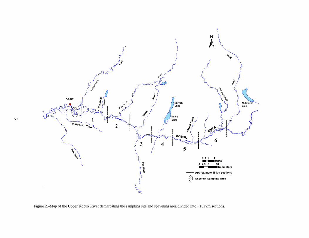
LIST OF FIGURES Figure Page 1. Map of the Kobuk and Selawik River drainages, Hotham Inlet, and Selawik Lake. ...................................... 2 2. Map of the Upper Kobuk River demarcating the sampling site and spawning area divided into ~15 rkm

sections. ........................................................................................................................................................... 5 3. A schematic of the joint live and dead encounters model ............................................................................. 12 4. Proportion of radiotagged male and female sheefish by 25 mm length category, 2008 and 2009. ............... 13 5. Map of the spawning area in the Upper Kobuk River demarcating the 2008–2014 spawning locations

of sheefish radiotagged in 2008 and 2009 ..................................................................................................... 15 6. Map of the Kobuk River demarcating the July 2009–2011 locations of sheefish ......................................... 18 7. Map of the Upper Kobuk River demarcating the temperature and habitat sampling locations in 2008

and 2014 ........................................................................................................................................................ 19 8. Temperature profiles from 3 data loggers located in the spawning area and the average downstream

migration timing of all radiotagged sheefish, 2008–2014. ............................................................................ 20 9. Downstream migratory timing of radiotagged sheefish past tracking stations, 2008–2009, 2011–2014. ..... 22 10. Upstream migratory timing of radiotagged sheefish past tracking stations, 2009, 2011–2013. .................... 23 11. Downstream migratory timing of female radiotagged sheefish past tracking stations, 2009, 2011–2014. ... 24 12. Downstream migratory timing of male radiotagged sheefish past tracking stations, 2009, 2011–2014. ...... 25 13. Upstream migratory timing of female radiotagged sheefish past tracking stations, 2009, 2011–2013. ........ 26 14. Upstream migratory timing of male radiotagged sheefish past tracking stations, 2009, 2011–2013. ........... 27 15. Number and proportion estimates without natural mortality, and 95% CIs of sheefish from each

tagging year returning to spawn by return year and sex. ............................................................................... 28 16. MLE proportion estimates from the JLD model and 95% CIs of sheefish from each tagging year

returning to spawn by return year. ................................................................................................................. 33 17. Bayesian proportion estimates from the JLD model and 95% CIs of sheefish from each tagging year

returning to spawn by return year. ................................................................................................................. 34 18. Spawning frequency estimates of male, female, and all radiotagged sheefish from 2008. ........................... 35 19. Spawning frequency estimates of male, female, and all radiotagged sheefish from 2009. ........................... 36

ii

ABSTRACT Radiotelemetry methods were used to document spawning locations, describe the timing of upstream and downstream spawning migrations, and estimate the spawning frequency of inconnu (sheefish) Stenodus leucichthys in the Kobuk River. In 2008 and 2009, 150 mature sheefish were captured each year and radiotagged from 17 July to 28 August. Aerial and stationary tracking data were used to document their spawning area, estimate the proportion that returned annually to spawn, and record their upstream and downstream migrations before and after spawning. Aerial tracking surveys were completed annually between July and October, 2008–2014. Numerous models were explored to estimate the annual proportion of sheefish that returned to spawn from each tagging year. The model chosen produced return proportion estimates that ranged from 0.33 (SE = 0.05) to 0.63 (SE = 0.07) for fish tagged in 2008, and 0.14 (SE = 0.03) to 0.80 (SE = 0.05) for fish tagged in 2009. The mean date of downstream passage (2008–2009, 2011–2014) ranged from 28 September in 2009 and 2014 to 5 October in 2012. The mean date of upstream passage (2009, 2011–2013) ranged from 21 August in 2011 to 4 September in 2013. Tracking station data from 2010 were lost because spring floods damaged the equipment. Sequential year spawning was documented for males and females in all years of the study. Sheefish exhibited a variety of spawning strategies but 32%–42% of males and 32%–37% of females spawned at least every other year. Key words: Kobuk River, inconnu, radiotelemetry, sheefish, spawning frequency, spawning location, spawning

migrations, Stenodus leucichthys

INTRODUCTION Inconnu Stenodus leucichthys, commonly known as sheefish in Alaska, are found in large rivers and associated lakes of northwestern North America and northeastern Asia as well as the White and Caspian Sea drainages (Berg 1948; Morrow 1980; Lee et al. 1980). Sheefish are an extremely important resource in northwest Alaska; their importance stems from their extensive use as a subsistence food, their value as a commercial resource, and their reputation as a trophy sport fish (Georgette and Loon 1990). There are only 2 known spawning populations that support the Northwest Alaska sheefish fisheries: one in the Upper Kobuk River; and the other in the Upper Selawik River near the confluence of Ingruksukruk Creek (Alt 1987; Figure 1). Over 20,000 sheefish are harvested annually throughout the Kobuk and Selawik River drainages; however, the majority of the harvest occurs during the winter subsistence fishery in Hotham Inlet and Selawik Lake where both stocks are mixed (Figure 1; Taube 1997; Savereide 2002).

Sheefish are the largest member of the whitefish subfamily Coregoninae and can be distinguished by their relatively large size, streamlined body, and extended lower jaw (Morrow 1980). They are iteroparous and usually mature around 8 to

12 years of age and can live for more than 30 years (Brown 2000; Howland et al. 2004). Their life history typically includes fall upriver migrations to freshwater spawning areas followed immediately by a downriver migration to overwintering and feeding areas within an estuary system; however, there are some stocks that do not exhibit these migrations and are considered resident populations (Alt 1987; Howland 1997; Brown 2000; Stuby 2012).

In particular, Kobuk River sheefish are estuarine anadromous, which means the majority of their life is spent in the brackish waters of Hotham Inlet (locally known as Kobuk Lake), Selawik Lake, and Kotzebue Sound (Smith et al. 2015). They are also known to be amphidromous, which means they migrate back and forth from the sea to fresh water looking for food. Young sheefish hatched in the Kobuk River do so during early spring before ice-out. After hatching, they are carried downstream by high spring flows to a wide array of destinations that include backwaters along the river, off-channel lakes, and the estuary regions mentioned above (Alt 1987). Juvenile sheefish feed mainly on insects and other small prey, but as they mature, they feed almost exclusively on fish including herring Clupea pallasi, smelt Osmerus mordax, lamprey Lampetra camtschatica, juvenile Dolly Varden Salvelinus malma, and various species of

1

2

Figure 1.–Map of the Kobuk and Selawik River drainages, Hotham Inlet, and Selawik Lake.

juvenile whitefish and Pacific salmon. Once mature, typically between age 5–9 for males and 7–12 for females, they return to their spawning grounds, which is described as a 90 km stretch of the mainstem Kobuk River from Kalla (an area ~10 km downstream from the Mauneluk River) upstream to the Reed River (Alt 1969; Figure 1). After spawning, the stock migrates back to the estuary system to overwinter and the cycle starts over.

Considerable research has been conducted on these stocks, with the first directed efforts initiated by the University of Alaska in the 1960s (Alt 1969). Since that time projects have been conducted to enumerate both spawning populations (Taube and Wuttig 1998; Underwood 2000; Hander et al. 2008), monitor region-wide harvests (Georgette and Loon 1990; Taube 1997; Savereide 2002), determine the composition of the mixed-stock winter fishery (Hander et al. In prep) and gather life history information (Miller et al. 1998).

Even with all of this information, the exploitation of these stocks is poorly understood. This is due to incomplete estimates of total annual harvest and unknown total exploitable stock abundance. The annual harvest (sport, commercial, and subsistence) is not assessed on a consistent basis (Table 1). In addition, the distribution of juveniles and adults throughout the estuary system coupled with the inability to differentiate stocks using genetics (Hander et al. In prep) makes it unfeasible to estimate total abundance using mark–recapture methodology.

An understanding of these basic elements is necessary to describe the population dynamics of each stock and identify sustainable harvest levels. However, before conducting additional spawning population assessments, a better understanding of spawning locations, run timing, and spawning frequency is required. The general consensus among scientists who study iteroparous fish in high latitudes is that most skip a year or more between spawning events because the energetic requirements of spawning in sequential years are too high (Alt 1969; Reist and Bond 1988; Lambert and Dodson 1990). Evidence of skip spawning has been observed in the Kobuk, Selawik, Yukon, and Kuskokwim

River populations (Alt 1987, Taube and Wuttig 1998, Underwood 2000; Brown and Burr 2012; Stuby 2012). Some Russian populations are believed to spawn every 3–4 years (Nikol’skii 1954), and Scott and Crossman (1973) suggested that some Canadian populations may spawn every 2–4 years. Because of this life history trait, estimates of spawning frequency are critical in determining whole population sizes based on spawning population estimates. In addition, describing the spawning locations and calculating estimates of run timing will provide the basis for improving and/or assessing the design of population assessment techniques like mark-recapture experiments or sonar.

OBJECTIVES The objectives for this study were to use radiotelemetry techniques to:

1. document spawning locations within the Kobuk River upstream of the village of Kobuk;

2. describe the timing of spawning migrations (upstream and downstream) for mature sheefish within the Kobuk River drainage;

3. estimate the proportion of the sheefish spawning population in 2008 and 2009 that return annually to spawning areas upstream of the village of Kobuk from 2009 to 2014; and

4. identify and characterize different spawning frequency strategies used by adult sheefish in the Kobuk River, estimate the proportion of adults using each strategy, and estimate the potential variation in the proportion of adult sheefish spawning in any given year.

METHODS Radiotelemetry techniques were used to estimate spawning frequency, document spawning areas, and estimate run timing (upriver and downriver migrations) of mature sheefish in the Kobuk River. Migrating fish were captured and radiotagged upstream of the village of Kobuk (Figure 2) to ensure that all fish sampled were mature and bound for upriver spawning areas. The duration of the migratory period past the

3

4

Table 1.–Reported and estimated commercial, sport, and subsistence sheefish harvests from Northwest Alaska communities and fisheries (sport and winter gillnet harvests were estimated, all other harvests were reported).

Subsistence

Sport

Community

Year Commercial

Northwest AKa

Kobuk River

Selawik River

Selawik Kobuk Noorvik Kiana Ambler Shungnak

Kobuk Drainage

Kotzebue Districtb

Winter Gillnet

1996 308 485 360 6,953 15,161 1997 0 906 304 9,805 13,704 1998 254 414 145 5,350 1999 635 621 8,256 2000 1,195 361 119 7,446 14,533 2001 19 1,305 552 59 3,838 2002 30 500 352 58 2,020 3,882 2003 122 2,509 676 0 7,823 2004 37 1,634 477 0 10,163 2005c 393 393 0 2006 0 810 566 0 5,129 1,298 2007 0 1,066 742 0 2008 0 61 0 0 2009 0 946 747 0 2010 0 595 86 221 2011 0 385 257 0 6,190 2012 0 104 50 0 1,062 6,032 1,156 1,556 2013 0 218 188 0 a Northwest Alaska includes all waters north of the Yukon River drainage in Norton Sound, the Seward Peninsula, and Kotzebue Sound. b Kotzebue District includes all waters flowing into Kotzebue Sound including the Kobuk, Noatak, and Selawik river drainages. c Less than 4 commercial deliveries, which is confidential under Alaska Statute 16.05.815. Prior to 2005, confidentiality was waived by permit holders.

5

Figure 2.–Map of the Upper Kobuk River demarcating the sampling site and spawning area divided into ~15 rkm sections.

capture site is known to last ~6 weeks from mid-July to late August, with the majority of the run passing during the first 3 weeks of August. Efforts were made to distribute radio transmitters over the entire duration of the run and in proportion to run strength to guard against potential differences in run-timing related to spawning areas (e.g., upper vs. lower reaches of spawning area) or spawning frequency. Sex-related differences in spawning behavior are more likely because of the higher energetic demands of producing eggs; therefore, attempts were made to distribute radio transmitters equally among males and females. Data related to movements, run timing, and spawning locations were collected using a combination of aerial tracking surveys and stationary tracking stations.

A 3-person crew was used to capture, sample, and radiotag 150 sheefish each year in 2008 and 2009. All sheefish were captured with hook and line gear. Radio transmitters were surgically implanted following the surgical methods detailed by Brown (2006) and Morris (2003). Radio transmitters were deployed in a systematic manner, and 2 h of fishing effort was expended at the capture site during each sampling day. For each sheefish radiotagged, data collected included:

1) measurement of fish length to the nearest 5 mm FL;

2) sex;

3) location (river-kilometer and GPS coordinate); and

4) date.

The 2008 deployment schedule (Table 2) was based on the approximate upstream migration past Kobuk village, which is just downstream of the capture site, and the 2009 schedule was based on catches observed in 2008. The first day of the run corresponded to the first day the crew caught a sheefish. The daily tagging schedule, angling effort, and sampling goals required adjustments based on perceptions of run timing and run strength using catch rates (current and prior years) and local knowledge.

Radio transmitters were distributed by sex and size. Sex was identified by inspecting external characteristics (i.e., gravidness and presence of swollen vent for females) or by examining the gonads through the incision. Because all fish were in spawning condition with fully developed gonads, all gonads were generally identifiable. In cases where sex could not be determined, no radio transmitter was inserted. Radio transmitters were nearly equally partitioned into 3 length categories, but because length composition can vary annually, minor adjustments to the length categories were needed. The categories were as follows: for males, ≤799 mm FL, 800-849 mm FL, and ≥850 mm FL; and for females, ≤899 mm FL, 900-974 mm FL, and ≥975 mm FL.

Implanted radio transmitters operated on 1 frequency for each year with individual transmitters digitally coded for identification. Transmitters were programmed to operate for 18 weeks per year (July through mid-November) transmitting 24 hours per day. Guaranteed transmitter operational life was 4 years, but potentially they could last up to 6 years.

Radiotagged sheefish were located using a combination of stationary tracking stations and aerial surveys. A combination of techniques is required to maximize the number of tagged sheefish detected on the spawning grounds and their upstream and downstream migration timing. Typically, a majority of the tagged fish are detected by the tracking stations and aerial surveys; however, fish can be detected on the aerial survey and not by the tracking stations and vice versa. For these reasons, multiple tracking stations and aerial surveys were conducted each year.

Three tracking stations were erected in 2008 to ensure that all fish migrating to and from spawning areas were identified. The farthest downstream station was located across from Kobuk and local students monitored and downloaded the information as part of their class work; the remaining 2 stations were located just upstream of Kobuk and downstream from the sampling site (Figure 2). In 2010, the farthest upriver station was removed and never replaced because spring flood conditions washed away

6

Table 2.–Number of radio transmitters deployed by day of run in 2008 and 2009.

2008 2009 Day of Runa Scheduled Actual Cumulative

Scheduled Actual Cumulative

1 1 1 1 1 1 1 2 2 2 3 2 2 3 3 2 1 4 2 2 5 4 2 3 7 2 2 7 5 2 2 9 2 2 9 6 2 2 11 2 2 11 7 2 2 13 2 2 13 8 2 2 15 2 2 15 9 2 2 17 2 2 17 10 2 2 19 2 2 19 11 2 2 21 2 3 22 12 3 3 24 3 1 23 13 3 3 27 3 4 27 14 3 3 30 3 5 32 15 3 3 33 3 5 37 16 3 3 36 3 4 41 17 3 3 39 3 4 45 18 3 3 42 3 3 48 19 3 3 45 3 2 50 20 4 4 49 4 4 54 21 4 4 53 4 4 58 22 4 4 57 4 2 60 23 4 3 60 4 1 61 24 4 5 65 4 9 70 25 4 4 69 4 6 76 26 5 5 74 5 5 81 27 5 5 79 5 5 86 28 5 5 84 5 5 91 29 5 5 89 5 7 98 30 5 5 94 5 6 104 31 5 5 99 5 7 111 32 5 5 104 5 7 118 33 5 5 109 4 7 125 34 4 4 113 4 6 131 35 4 4 117 4 6 137 36 4 4 121 4 5 142 37 4 4 125 4 3 145 38 4 4 129 4 2 147 39 4 4 133 4 2 149 40 4 4 137 4 1 150 41 4 4 141 3 0 150

42 3 3 144 3 0 150 43 3 6 150 3 0 150 44 3 0 150 2 0 150 45 0

0 150 2 0 150

46 0 0 150 1 0 150 a Day 1 corresponded to the first day a sheefish was caught.

7

the cut-bank where the station was located and the remaining 2 stations located all of the fish recorded on the third. Each station included a deep-cycle battery, a solar array, an antenna switch box, a steel housing box, 2 Yagi antennas, and a Lotek SRX 600 receiver and data logger. The tracking stations were operational between July and November. The receiver monitored the frequencies continuously and received from all antennas simultaneously. When a signal of sufficient strength was encountered, the receiver would pause for 8 s on each antenna, and then transmitter frequency, transmitter code, signal strength, date, time, and antenna number were recorded on the data logger. Depending on the swimming speed of the tagged fish, this configuration allowed the data logger to record multiple radiotagged sheefish migrating past the tracking station at the same time.

A series of aerial tracking surveys (2–5 each year) over the spawning area during the spawning period, which were believed to extend from Kalla to the Reed River during late September through early October (Alt 1987; Taube and Wuttig 1998; Figure 1), were conducted from a small fixed-wing aircraft from mid-July to early October. Tracking surveys in July and August were performed to document the upstream migration of radiotagged sheefish from Hotham Inlet to spawning and/or feeding areas. Tracking surveys were done in cooperation with the U.S. Fish and Wildlife Service.

Site visits to the lower and middle reaches of the spawning area were conducted in 2008 and 2014 to collect water quality data. Spawning habitat characteristics were measured using a HACH HQ Series portable meter and a Flow Probe FP101 to acquire water temperature, flow rate, dissolved oxygen, pH, and conductivity. A Secchi disk was used to discern water transparency. In addition, 6 Hobo v2 temperature data loggers were deployed to record temperature changes before, during, and after the spawning period.

DATA ANALYSIS Spawning Locations

From 2008 through 2014, aerial surveys conducted throughout the spawning area were used to document the maximum upstream extent sheefish were located. The spawning area was partitioned into 6 sections of river ~15 rkm and each section was weighted by the proportion of transmitters present to identify patterns in fish densities (Figure 2). Contingency table analysis using chi-square tests were performed to explore for independence of spawning location and year. The partitioning was examined for each year and over all years pooled to identify any variation in the selected spawning area.

Run Timing

For all fish migrating past the tracking stations, an upstream and downstream run-timing profile was constructed. Contingency table analysis using chi-square tests were performed to explore for independence of migratory timing and sex. For example, the ratio of males to females from the beginning of the downstream migration until the mean date of passage were compared to the ratio from the mean date of passage to the end of the downstream migration. A generalized description of migratory patterns along the length of their migration from Hotham Inlet to their spawning area and back (i.e., from July through October) was developed using data from all aerial surveys and tracking stations.

Run timing profiles were described as time-density functions, where the relative abundance of sheefish migrating upstream and downstream of the tracking stations during time interval t were described by (Mundy 1979):

( )∑=

= T

tt

t

R

Rtf

1

(1)

where:

f (t) = the empirical temporal probability distribution over the total span of the spawning migration (upstream and downstream)

8

for sheefish spawning in the Kobuk River; and,

tR = the subset of radiotagged sheefish that migrated past the tracking stations during day t.

The mean date of passage ( t ) past the tracking stations (upstream and downstream) were estimated as:

( )∑=t

tftt , (2)

the variance of the mean date of passage was estimated as:

( ) ( )

∑

∑

=

=

−= T

tt

T

t

R

tftttVar

1

2

1)( . (3)

Spawning Frequency

To facilitate data analysis, all radiotagged sheefish were assigned a “fate” (Table 3). The known fates of all radio transmitters are required to attain unbiased parameter estimates. Fates were determined from a combination of information collected from tracking stations, aerial tracking surveys, “ground-truthing” of radio transmitters with suspect fates (harvested and not reported), and harvested fish for which radio transmitters were returned.

Mortality can be easily inferred because sheefish are highly migratory. In other words, if a sheefish is located twice and fails to move a significant distance (e.g., 10 rkm) over a period of 1 month or greater, then it is likely to have died or lost the transmitter. In contrast, accounting for all non-spawners could be problematic because radio transmitters cannot transmit through the brackish waters of Hotham Inlet where they seasonally reside for foraging during years when they do not spawn. However, a number of non-spawning sheefish enter the lower portions of the Kobuk River and Selawik Lake during the open-water period to forage (Alt 1987), which makes it possible to locate them from the air. Because natural mortality is

thought to be minimal during summer, fish that were located at least once would have likely survived to the fall, and therefore would be considered to have been alive at the time of spawning for that year. Non-reporting of a radiotagged sheefish in the subsistence and sport fisheries could occur, but tagging studies in the area indicate that the majority of fishermen report tagged fish in their harvest. In addition, unreported harvested fish were easily deduced during aerial surveys. Radio transmitters removed from the water have a sharp increase in their signal strength and range, and a non-reported harvest was inferred if such a transmitter was located from the air within a village, established fish camp, or cabin.

To further aid in accounting for all fates, radio transmitters had return information printed on them and a monetary reward was offered. Local residents voiced their support for this project and good cooperation and reporting was expected if transmitters were caught. Informational flyers and posters describing the project and encouraging transmitter returns were posted in all villages where harvests may have occurred and announcements were made at appropriate stakeholder meetings and over the radio.

Attaining unbiased estimates assumes that the behavior expressed by radiotagged sheefish is the same as that of the untagged population. There was no explicit test for this assumption because we cannot observe the behavior of unhandled fish. However, sheefish surviving until the following open-water period would be used as evidence that the stress of bearing radio transmitters had abated and spawning-related behavior (run timing, selection of spawning area, and spawning frequency) was representative of the population.

To estimate the proportion of sheefish spawning in a given year, we explored 3 different models. The first, considered the basic model, estimated the proportion of sheefish spawning in a given year and its variance (Cochran 1977) as:

t

tt n

xp =ˆ (4)

9

10

Table 3.–List of possible fates of radiotagged sheefish in the Kobuk River.

Fate Description

Unknown (U) A fish that was never located because of radio transmitter failure or could never be located after tagging. Fish with this fate were culled from the data set.

Tagging Mortality (TM) A fish that died in response to transmitter implantation prior to the first aerial survey. Fish with this fate were culled from the data set.

Fishing Mortality (FM) In a given year, a fish reported harvested in one of the fisheries prior to passing the tracking station near the village of Kobuk.

Indefinite (I) A sheefish that was alive the prior year but was never located during a subsequent year. These fish were either alive or dead but not enough information existed to designate them as S or NS.

Spawner (S) In a given year, a fish that migrated past the tracking station near Kobuk and either died immediately thereafter due to fishing or natural mortality, a fish that completed its upstream and downstream spawning migration, or based on several observations (e.g., 4 surveys during the summer/fall), a fish that displayed an obvious migration pattern towards the spawning area.

Non-Spawner (NS) In a given year, a fish that was located at least once during the summer in the lower portions of the Kobuk or Selawik rivers but did not pass the tracking station at Kobuk, a fish that did not display an obvious migration pattern towards the spawning area, or a fish that was not located and judged to be alive (e.g., returned to spawn) in subsequent years.

1np1ppV

t

ttt

)ˆ(ˆ)ˆ(ˆ (5)

where:

tp̂ = the proportion of sheefish spawning in

year t;

tx = the number of sheefish with fate (S) in

year t; and

nt = all sheefish with fate (S), (NS), and (I) in year t.

Ninety percent confidence intervals around tp̂were calculated using exact binomial confidence limits (Cochran 1977). These estimates account for fishing mortality because all harvested fish were accounted for and culled from the analysis; however, the estimates could be biased low because fish with fate (I) can be alive or dead from natural mortality. Brown and Burr (2012) estimated Innoko River sheefish annual survival using historical age data and a catch curve procedure outlined by Robson and Chapman (1961). Even though this procedure is logical and relatively accurate, the derived estimate of

total mortality (37%) would not be plausible for sheefish in the Kobuk River. In fact, applying a fixed total mortality rate of 20% results in culling radiotagged sheefish from the analysis that are known to still be alive.

Fitting mark and recapture models to our data was a second way we estimated spawning and mortality rates. The Cormack-Jolly-Seber (CJS) model for open populations is a restricted version of the Jolly-Seber model that allows for specific estimates of apparent survival ϕ and the probability of capture/recapture p. The model assumptions are as follows: 1) tagged fish are representative of the population; 2) fish must retain their tags; 3) tagging does not affect the behavior of fish; and 4) every fish must have an equal probability of being tagged/recaptured during each event or all tagged fish mix completely with unmarked fish. The capture history takes the form of LLLLL depending on the number of occasions and whether an individual is captured (L = 1) or not (L = 0). For example, a capture history of 10101 means a fish was captured during the first, third, and fifth occasions and was not captured during the second and fourth. In our case, we assumed the

probability of a radiotagged fish being detected on the spawning grounds was 100%; therefore, the capture probability depicted in the CJS model is equivalent to the probability of a sheefish returning to spawn given that it survived the previous year. The CJS model data only reflect live encounters. This means that individuals with a 0 or multiple 0 designations in their capture history were just not present on the spawning grounds; however, over the course of our study we know some of these fish were captured in the subsistence fishery or died from natural mortality, and this information cannot be incorporated in the CJS model.

The third model we used was a joint live and dead encounters (JLD) model developed by Burnham (1993) and contained within the program MARK (White and Burnham 1999) that incorporated dead recovery information into the estimation of spawning frequency. The assumptions of this model are the same as the CJS model. The difference between the joint model and the live recaptures model is the recapture history for the joint model is in pairs for each occasion. The input data takes the form of a mark–recapture experiment where sheefish encountered on the spawning grounds in any particular year are considered a live encounter and any known mortality between spawning events is a dead encounter. The data input takes the form of LDLD, where L = 1 when a fish is encountered alive on the spawning grounds and L = 0 when not encountered, and when a fish is not encountered between spawning events D = 0 and when found dead D = 1. For example, a sheefish found on the spawning grounds in year 1 and 2 but reported dead after spawning in year 2 would have a capture history of 10 in year 1 and 11 in year 2, or 1011. A schematic of the model and its parameters illustrates the model structure (Figure 3).

There are 4 parameters in the JLD model: S for survival probability, F for fidelity to the area, p for recapture probability, and r for the probability of being reported if a fish is dead. In the context of this study, the recapture probability p equates to the proportion that returns to spawn and 1-S equals the probability a radiotagged sheefish does not survive to the next spawning event.

Two scenarios of the JLD model were explored (constant S and varying S) in a maximum likelihood (MLE) and Bayesian (implemented by Markov Chain Monte Carlo MCMC) framework. The r parameter in the last year was fixed at zero because there was no information available after that time to determine whether a fish was alive or dead. In other words, the r parameter is derived from reported mortalities between spawning events and there were no efforts to acquire mortality information after the last spawning event, so the probability of reporting fish mortality is set to zero. Fidelity to the spawning area F was fixed at 1.0 because multiple tagging studies, including this one, have shown that Kobuk and Selawik River sheefish stocks only spawn in their respective natal streams (Taube and Wuttig 1998; Underwood 2000).

The most appropriate scenario in the maximum likelihood setting was chosen using the Akaike Information Criterion (AIC) that measures the relative quality of statistical models for a given set of data; the model with the lowest AIC score is considered to best represent the data with the fewest parameters.

The program MARK has 4 options for estimating the variance-covariance matrix of the model’s parameters: 1) the inverse of the Hessian matrix obtained from a numerical optimization of the likelihood function; 2) an information matrix determined by the numerical derivatives of the probabilities of each capture history; 3) an information matrix determined by the expected values of the probabilities of each capture history; and 4) an information matrix using central difference approximations of the second partial derivatives (White and Burnham 1999). The second partial derivative method is preferred because it provides more accurate estimates of the standard errors, and the program sets it as the default method.

The program also has a number of functions that “link” the linear model specified in the design matrix to the parameters of the model. The link functions allow parameters between zero and one to be transformed, so they can vary between ± infinity, in order to fit the linear regression model in MARK.

11

Three linanalysis aaffected plogistic linthe most a

Spawning

If distinctobserved between sspawn moyear), thdescribedeach stratby:

s

ss n

xp ˆ

pV sˆ(ˆ

where:

sp̂ =

sx =

ns =

Figure 3.–

k functions wand the resultparameter esnk function wappropriate fu

g Frequency S

t spawning f(i.e., some fis

spawning eveore regularly hen the in. The proportegy and its

n1p

s

s(ˆ

)

the proport

spawning y

the numbe

spawning y

total numbe

–A schematic o

were explorets revealed th

stimates of vwas chosen bunction based

Strategies

frequency strsh consistentl

ents while othskipping eve

ndividual partion of adulvariance we

1p1

s

s

)ˆ

tion of shee

times over t y

er of sheef

times over t y

er of sheefish

of the joint live

ed during thehat they onlyvariance. Theecause it was

d on the data.

rategies werely skip 1 yearhers appear toery 3rd or 4thatterns werelts exhibiting

ere calculated

(5)

(6)

efish (sex s)

years;

fish (sex s)

years; and

(sex s).

12

e and dead enc

e y e s

e r o h e g d

)

)

A toand fromwere2009radiothe dand femadownd.f. =downd.f. =p = 0

Spaw

A nucondinrivradionumsheeRiveKallacondweretimenot jradioto be

counters model

otal of 150 msurgically im

m 17 July to 3e implanted 9 (Table 2).otagged sheedifference infemales (Fig

ales was simnstream mea= 1, p = 0.86nstream mea= 1, p=0.48 0.80 downstre

wning Locati

umber of annuducted from 2ver spawningotagged fish

mber located vefish were fouer and downa (Figure 5).

ducted in 20e expected toe and money justified. Thotagged fish,e justified.

l (Burnham 19

RESULTSmature sheef

mplanted with0 August 200during 18 Ju Length com

efish from ean length betwgure 4). The

milar before aan date of p6) and the 20an dates of p

upstream; χeam).

ions

ual aerial trac2008 to 2014g and feed

h (Table 4; varied each yund as far upsnstream to an. Only 2 trac

014 because o start shuttirequired for

he 2014 flighso this assu

93).

S fish were caph radio transm08 and anotheuly to 28 Ampositions oach year illu

ween mature ratio of ma

and after the passage (χ2 =009 upstreampassage (χ2 =χ2 = 0.07, d.f

cking surveys4 to determinding location

Figure 5). year but spawstream as the n area just bcking flights radio transm

ing down an3 to 5 flight

hts only founumption turne

ptured mitters er 150

August of the ustrate males les to 2008

= 0.03, m and = 0.49, f. = 1,

s were ne the ns of

The wning Reed below

were mitters nd the ts was nd 14 ed out

13

Figure 4.–Proportion of radiotagged male and female sheefish by 25 mm length category,

2008 and 2009.

0.00

0.05

0.10

0.15

0.20

0.25

675 725 775 825 875 925 975 1025

Pro

port

ion

of s

heef

ish

Length Categories (mm)

2008

Males

Females

0.00

0.05

0.10

0.15

0.20

0.25

0.30

675 725 775 825 875 925 975 1025 1075

Pro

port

ion

of s

heef

ish

Length Categories (mm)

2009

Males

Females

Table 4.–Tracking flights, dates, and number of sheefish located by year.

Number of flights

Date range

Number located

2008 5 9/3 - 9/30 81 2009 5 7/23 - 9/30 70 2010 4 7/26 - 9/29 44 2011 3 7/22 - 9/28 47 2012 5 7/3 - 10/9 71 2013 4 7/19 - 10/4 24 2014 2 7/21 - 10/3 14

Table 5.–P-values from contingency tests

comparing radiotagged fish located in the 6 reaches of the spawning area from year to year and combined (bold values are significant).

2008 2009 2010 2011 2012 2013 2014 2009 0.07 - - - - - - 2010 <0.00 0.82 - - - - - 2011 0.02 0.80 0.96 - - - - 2012 <0.00 0.26 0.69 0.69 - - - 2013 0.14 0.96 0.97 0.99 0.76 - - 2014 0.07 0.81 0.96 0.92 0.82 0.97 - All Years 0.67 0.58 0.07 0.18 <0.00 0.58 0.33

14

15

Figure 5.–Map of the spawning area in the Upper Kobuk River demarcating the 2008–2014 spawning locations of sheefish radiotagged in 2008 and 2009

(vertical lines indicate ~15 km sections).

A series of contingency tests indicated the number of radiotagged fish located in the 6 reaches of the spawning area were similar from year to year and across all years more often than they were different (Table 5). The largest proportions of radiotagged sheefish were located in sections 3, 4, and 5 (Table 6).

Radiotagged fish located inriver during July (2009–2013) were either migrating up to their spawning grounds or feeding at or near the mouths of a number of chum salmon Oncorhynchus keta, whitefish, and Dolly Varden spawning/rearing tributaries (Figure 6). Sheefish that did not spawn in a particular year were located in the same areas as sheefish that continued upstream to spawn that year (Figure 6).

Basic water quality characteristics were collected from the middle and lower reaches of the spawning area in 2008 and 2014. Three of the 6 temperature loggers deployed in the spawning area during 2008 were lost due to ice scouring during spring breakup; however, 3 were retrieved during August 2009 (Figure 7). The temperature profiles from these loggers illustrate the temperature drop that triggers the spawning event (Figure 8). Seven sampling sites revealed that pH values ranged from 7.75 to 8.57, conductivity ranged from 76.4 to 168.7 µS/cm, and temperature ranged from 6.70 to 8.63 °C (Figure 7; Table 7). Turbidity measured from a Secchi disk revealed that depths greater than 1.5 m were easily achieved (Table 7).

Run Timing

Tracking stations were downloaded 2 to 3 times during late September and early October, using satellite modems, which worked very well except in 2010; a blown fuse in one modem and an animal-damaged power cord on the other modem precluded remote data collection. The situation worsened the following spring when an early ice breakup and strong winds prevented the project leader from retrieving the tracking station equipment before an ice jam near Kobuk village caused serious flooding; the equipment was recovered and repaired but unfortunately all the run-timing data for the 2010 season was lost. In 2014, a conflict between the radio transmitters and software in the receivers

recorded nonsensical data during the upstream migration from 15 July through 4 September; the software conflict was corrected on 5 September.

The mean date of downstream migration from 2008 to 2014 varied from 29 September to 6 October (Table 8; Figure 9). The mean date of upstream migration from 2009 to 2013 varied from 22 August to 5 September (Table 8, Figure 10). The longest downstream migration was in 2013 and lasted 50 days, whereas the longest upstream migration was in 2011 and lasted 85 days (Table 8). Upstream and downstream migration timing was also determined by sex where mean dates of passage were similar, but females did tend to arrive later to the spawning grounds (Table 8; Figures 11–14).

Spawning Frequency

Proportion estimates of sheefish from each tagging year that returned to spawn in 2014 are not presented because the number that returned was small and biased low due to the radio transmitters’ life span. The transmitters were guaranteed to transmit for 4 years; the number returning from each tagging year suggests that the majority of the 2008 transmitters effectively lasted 5 years whereas the majority of 2009 transmitters only lasted 4 (Figure 15 Panel A).

Sequential year spawning was observed by males and females in all years of the study. After their year of tagging, 60–67% of males returned to spawn the following year. In contrast, only 33–40% of females returned to spawn the year after being radiotagged (Figure 15 Panel B).

The return proportion estimates from the basic model varied by return year and sex with a higher proportion of males returning annually to spawn (Table 9, Figure 15 Panel C). Annual return proportions for all fish ranged from 0.13 to 0.68, whereas return proportions for females ranged from 0.26 to 0.51 and 0.49 to 0.74 for males.

16

Table 6.–Number and percentage of radiotagged sheefish located by section within the spawning area, 2008–2014.

2008 2009 2010 Area # Located Percentage Area # Located Percentage

Area # Located Percentage

1 4 4.9%

1 8 11.4% 1 7 15.9% 2 6 7.4%

2 9 12.9%

2 6 13.6%

3 25 30.9%

3 20 28.6%

3 10 22.7% 4 9 11.1%

4 15 21.4%

4 13 29.5%

5 30 37.0%

5 13 18.6%

5 6 13.6% 6 7 8.6%

6 5 7.1%

6 2 4.5%

Total 81 Total 70 Total 44

2011

2012

2013 Area # Located Percentage Area # Located Percentage

Area # Located Percentage

1 6 12.8%

1 5 7.0%

1 3 12.5% 2 6 12.8%

2 9 12.7%

2 4 16.7%

3 9 19.2%

3 17 23.9%

3 5 20.8% 4 14 29.8%

4 28 39.4%

4 6 25.0%

5 10 21.3%

5 10 14.1%

5 5 20.8% 6 2 4.3%

6 2 2.8%

6 1 4.2%

Total 47 Total 71

Total 24

2014 Area # Located Percentage 1 2 14.3% 2 3 21.4% 3 3 21.4% 4 4 28.6% 5 2 14.3% 6 0 0% Total 14

17

18

Figure 6.–Map of the Kobuk River demarcating the July 2009–2011 locations of sheefish. Diamond symbols represent fish that were located at

feeding areas in July and did not spawn in that particular year, but did spawn in a following year. Ovals represent fish that did spawn in that particular year.

Figure 7.–Map of the Upper Kobuk River demarcating the temperature (●) and habitat (◊) sampling locations in

2008 and 2014 (the campsite is lowest point on the river where radiotagged sheefish were located during spawning).

19

Figure 8.–Temperature profiles from 3 data loggers located in the spawning area (2008) and the average downstream migration timing of all radiotagged sheefish, 2008–2014.

Table 7.–Habitat characteristics recorded from the Kobuk River spawning area, 2014.

Date/Time Site pH Temperature

oC Conductivity

µS/cm

Secchi Deptha

m Flow Rate

m/sec

Pah River 9/14/14 13:40 1 7.75 6.70 76.4 - -

Kobuk River 9/14/14 14:00 2 8.01 8.25 154.6 1.2+ - 9/14/14 14:30 3 7.90 7.40 88.6 1.5+ 0.50 9/14/14 15:20 4 8.54 8.57 146.1 1.5+ 0.50 9/14/14 14:00 5 8.57 8.63 153.3 1.5+ - 9/14/14 14:00 6 7.95 8.20 166.5 1.5+ - 9/14/14 14:00 7 8.23 8.10 168.7 1.5+ -

a It was not possible to keep the Secchi disk vertical in the water column because of strong current; however, Secchi depths of 1.5 m were easily discernable.

0.00

0.25

0.50

0.75

1.00

0

2

4

6

8

10

12

14

16

8-Aug 28-Aug 17-Sep 7-Oct 27-Oct

Cum

ulative percentage Te

mpe

ratu

re °C

Temp Logger 1

Temp Logger 2

Temp Logger 3

Downstream Average

20

21

Table 8.–Mean dates of upstream and downstream passage, dates of first and last fish, and duration of migration in days for all fish, females, and males from 2008 to 2014.

Downstream Migration Upstream Migration

All Fish Mean Date First Fish Last Fish Duration

All Fish Mean Date First Fish Last Fish Duration

2008 2-Oct 14-Sep 17-Oct 33

2009 3-Sep 1-Aug 29-Sep 59

2009 28-Sep 5-Sep 8-Oct 33

2011 21-Aug 7-Jul 30-Sep 85

2011 2-Oct 4-Sep 8-Oct 34

2012 3-Sep 11-Aug 28-Sep 48

2012 5-Oct 17-Sep 18-Oct 31

2013 4-Sep 28-Aug 19-Sep 22

2013 29-Sep 16-Sep 5-Nov 50

2014 28-Sep 13-Sep 5-Oct 22

Female Mean Date First Fish Last Fish Duration

Female Mean Date First Fish Last Fish Duration 2008 1-Oct 17-Sep 15-Oct 28

2009 5-Sep 8-Aug 29-Sep 52

2009 27-Sep 5-Sep 8-Oct 33

2011 22-Aug 7-Jul 24-Sep 79 2011 30-Sep 4-Sep 8-Oct 34

2012 6-Sep 11-Aug 27-Sep 47

2012 5-Oct 17-Sep 17-Oct 30

2013 6-Sep 30-Aug 17-Sep 18 2013 4-Oct 22-Sep 5-Nov 44

2014 28-Sep 16-Sep 5-Oct 19

Male Mean Date First Fish Last Fish Duration

Male Mean Date First Fish Last Fish Duration 2008 2-Oct 14-Sep 17-Oct 33

2009 3-Sep 1-Aug 29-Sep 59

2009 29-Sep 11-Sep 8-Oct 27

2011 20-Aug 7-Jul 30-Sep 85 2011 3-Oct 22-Sep 8-Oct 16

2012 1-Sep 11-Aug 28-Sep 48

2012 5-Oct 25-Sep 18-Oct 23

2013 2-Sep 28-Aug 19-Sep 22 2013 27-Sep 16-Sep 2-Oct 16

2014 28-Sep 13-Sep 2-Oct 19

Figure 9.–Downstream migratory timing of radiotagged sheefish past tracking stations, 2008–2009,

2011–2014.

0.00

0.25

0.50

0.75

1.00

29-Aug 8-Sep 18-Sep 28-Sep 8-Oct 18-Oct 28-Oct 7-Nov

Cum

ulat

ive

prop

ortio

n

Downstream migration date past tracking stations

200820092011201220132014Average

22

Figure 10.–Upstream migratory timing of radiotagged sheefish past tracking stations, 2009, 2011–2013.

0.00

0.25

0.50

0.75

1.00

24-Jun 14-Jul 3-Aug 23-Aug 12-Sep 2-Oct

Cum

ulat

ive

prop

ortio

n

Upstream migration date past tracking stations

2009201120122013Average

23

Figure 11.–Downstream migratory timing of female radiotagged sheefish past tracking stations, 2009,

2011–2014.

0.00

0.25

0.50

0.75

1.00

29-Aug 8-Sep 18-Sep 28-Sep 8-Oct 18-Oct 28-Oct 7-Nov

Cum

ulat

ive

prop

ortio

n

Female downstream migration date past tracking staions

200820092011201220132014Average

24

Figure 12.–Downstream migratory timing of male radiotagged sheefish past tracking stations, 2009,

2011–2014.

0.00

0.25

0.50

0.75

1.00

29-Aug 8-Sep 18-Sep 28-Sep 8-Oct 18-Oct 28-Oct 7-Nov

Cum

ulat

ive

prop

ortio

n

Male downstream migration date past tracking staions

200820092011201220132014Average

25

Figure 13.–Upstream migratory timing of female radiotagged sheefish past tracking stations, 2009,

2011–2013.

0.00

0.25

0.50

0.75

1.00

30-Jun 10-Jul 20-Jul 30-Jul 9-Aug 19-Aug 29-Aug 8-Sep 18-Sep 28-Sep

Cum

ulat

ive

prop

ortio

n

Female upstream migration date past tracking stations

2009

2011

2012

26

Figure 14.–Upstream migratory timing of male radiotagged sheefish past tracking stations, 2009, 2011–2013.

0.00

0.25

0.50

0.75

1.00

30-Jun 10-Jul 20-Jul 30-Jul 9-Aug 19-Aug 29-Aug 8-Sep 18-Sep 28-Sep

Cum

ulat

ive

prop

ortio

n

Male upstream migration date past tracking stations

2009

2011

2012

2013

27

Figure 15.–Number (Panel A) and proportion estimates without natural mortality, and 95% CIs

(Panels B and C) of sheefish from each tagging year returning to spawn by return year and sex.

0

10

20

30

40

50

60

70

80

2009 2010 2011 2012 2013 2014

Num

ber r

etur

ning

to sp

awn

Return year

Panel A

Tagged in 2008

Tagged in 2009

0.00

0.25

0.50

0.75

1.00

2009 2010 2011 2012 2013

Prop

ortio

n re

turn

ing

to sp

awn

Return year

Panel B

Tagged in 2008

Tagged in 2009

0.000.100.200.300.400.500.600.700.800.901.00

Female Male Female Male

Tagged 2008 Tagged 2009

Prop

ortio

n re

turn

ing

to sp

awn Panel C 2009 2010 2011 2012 2013

28

Table 9.–Number and proportion estimates from each tagging year of sheefish returning to spawn from the basic model by return year and sex.

Tagged in 2008

All Fish

Females

Males

Return Year Number

Proportion SE

Proportion SE

Proportion SE 2009 64

0.56 0.05

0.33 0.06

0.67 0.06

2010 32

0.29 0.04

0.34 0.09

0.66 0.09 2011 40

0.37 0.05

0.35 0.08

0.65 0.08

2012 51

0.47 0.05

0.39 0.07

0.61 0.07 2013 38 0.35 0.05 0.26 0.07 0.74 0.07

Tagged in 2009

All Fish

Females

Males

Return Year Number

Proportion SE

Proportion SE

Proportion SE

2009 2010 15

0.13 0.03

0.40 0.13

0.60 0.13

2011 56

0.50 0.05

0.48 0.07

0.52 0.07 2012 75

0.68 0.04

0.51 0.06

0.49 0.06

29

The proportion returning annually to spawn from the JLD models also varied by return year, but similar patterns were observed (Tables 10–11, Figures 16–17). Return proportion estimates ranged from 0.13 to 0.80 for all fish. The estimates from the JLD models were not broken down by sex because of the similarities across years compared to the basic model and the fact that the length compositions and run-timing patterns suggest that radiotagged sheefish of both sexes were representative of the spawning stock.

The survival probability estimates from both scenarios and estimators of the JLD model are similar for each tagging year (Tables 10–11). They range from 0.88 to 0.91 for the constant S scenarios and 0.78 to 0.98 for the varying S scenarios (Tables 10–11). Even though these are not estimates of apparent survival, they do reflect the probability that a fish survived between spawning events, while accounting for all forms of mortality.

The model with the lowest AIC score using the MLE was the constant S scenario. The varying S scenarios were unable to estimate SEs for some of the estimates of S, p, and r (Tables 10–11), which is why the AIC scores indicated that the constant S scenarios fit better. In contrast, the Bayesian (MCMC) estimator was able to produce sensical variance estimates for all parameters, but with larger CIs in later years (Tables 10–11).

Spawning Frequency Strategies

The proportion of sheefish that exhibited a particular spawning strategy illustrates that males spawn more often, whereas the majority of females spawn every other year (Figures 18 and 19). The proportion that spawned at least 50% of the time ranged from 0.32 to 0.42 for males and 0.31 to 0.37 for females. The proportion that returned to spawn at least 80% of the time was ~0.17 for males and females (Figures 18 and 19).

DISCUSSION Previous studies and local knowledge have established that sheefish in the Kobuk River tend to reach spawning areas upstream from Kobuk village by late August (Alt 1987, Taube and

Wuttig 1998). Capturing and radiotagging 150 sheefish in 2 consecutive years just upstream from Kobuk for approximately 6 weeks before the end of August ensured that a representative proportion of the spawning population was sampled (Table 6).

Efforts were also made to deploy radio transmitters in proportion to their upstream migration, sex, and length. Length compositions of the radiotagged sheefish (Figure 4) are normally distributed and suggest a representative sample of the spawning stock. In addition, contingency tests revealed that the ratio of males to females before and after the mean dates of passage were similar, which implies both sexes were tagged proportionally to their downstream and upstream migrations.

Spawning Locations

Habitat characteristics like water temperature and substrate composition limit available spawning areas. Sheefish have specialized spawning habitats that possess similar geologic landscapes among different tributaries throughout their natural range (Alt 1987; Howland 2005; Gerken 2009; Stuby 2012). The areas all contain specific geologic features that are associated with specific water quality characteristics like pH, temperature, and conductivity (Brabets et al. 2000). A combination of limestone, dolomite, and sandstone is common to all of the known spawning areas on the Alatna, Selawik, Sulukna, Kuskokwim, Selawik, and Kobuk rivers (Beikman 1980; Gerken 2009; Stuby 2012).

Studies have shown that sheefish prefer habitat composed of differentially sized sediments with varying degrees of distribution, area, and proportions of cobble, gravel, and sand, which describes the composition in the Kobuk River spawning area (Alt 1987; Gerken 2009; Stuby 2012). In addition, Alt (1987), Howland (2005), Gerken (2009), and Stuby (2012) have all noted that sheefish prefer water temperatures between 0°C and 6°C for spawning; the temperature profiles (Figure 8) collected during this study coupled with estimates of run timing (Figures 9–14) demonstrate that this is also true for the Kobuk River spawning stock.

30

Table 10.–Number and proportion estimates from the JLD model of sheefish returning to spawn from tagging year 2008.

Maximum Likelihood Estimator Scenario 1: Constant S, F = 1

Tagged in 2008

All Fish

Survival

Reported Dead

Return Year Number

Proportion SE

S SE

r SE 2009 64

0.57 0.05

0.88 0.02

0.79 0.17

2010 32

0.32 0.05

0.23 0.13 2011 40

0.47 0.06

0.15 0.11

2012 51

0.64 0.07

0.10 0.10 2013 38 0.53 0.08 0.000000012 0.000039

Scenario 2: Varying S, F = 1 Tagged in 2008

All Fish

Survival

Reported Dead

Return Year Number

Proportion SEa

S SEa

r SE 2009 64

0.58 0.05

0.85 0.04

0.70 0.17

2010 32

0.30 0.05

0.97 0.02

0.99 0.13 2011 40

0.48 0.06

0.78 0.07

0.08 0.11

2012 51

0.63 0.08

0.92 0.11

0.19 0.10 2013 38 0.58 0.00 0.78 0.00 0.000000041 0.000049

Bayesian Estimator Scenario 1: Constant S, F = 1 Tagged in 2008

All Fish

Survival

Reported Dead

Return Year Number

Proportion SD

S SD

r SD 2009 64

0.57 0.05

0.88 0.02

0.77 0.13

2010 32

0.33 0.05

0.28 0.14 2011 40

0.46 0.06

0.22 0.13

2012 51

0.63 0.07

0.18 0.13 2013 38 0.52 0.08 0.11 0.09

Scenario 2: Varying S, F = 1

Tagged in 2008

All Fish

Survival

Reported Dead

Return Year Number

Proportion SD

S SD

r SD 2009 64

0.58 0.05

0.85 0.04

0.72 0.15

2010 32

0.32 0.05

0.92 0.05

0.48 0.25 2011 40

0.47 0.06

0.83 0.07

0.19 0.16

2012 51

0.62 0.07

0.90 0.14

0.3 0.24 2013 38 0.54 0.13 0.86 0.30 0.19 0.23

a Numbers in bold designate parameter estimates without SEs.

31

Table 11.–Number and proportion estimates from the JLD model of sheefish returning to spawn from tagging year 2009.

Maximum Likelihood Estimator Scenario 1: Constant S, F = 1

Tagged in 2009

All Fish

Survival

Reported Dead

Return Year Number

Proportion SE

S SE

r SE 2010 32

0.13 0.03

0.91 0.02

0.96 0.24

2011 40

0.55 0.05

0.20 0.14 2012 51

0.80 0.05

0.0000000003 0.0000029

2013 38 0.45 0.06 0.35 0.21

Scenario 2: Varying S, F = 1 Tagged in 2009

All Fish

Survival

Reported Dead

Return Year Number

Proportion SEa

S SEa

r SEa

2010 32

0.15 0.04

0.82 0.04

0.52 0.13 2011 40

0.56 0.05

0.98 0.01

1.00 0.00

2012 51

0.78 0.06

0.96 0.07

0.000000077 0.00014 2013 38 0.60 0.00 0.66 0.00 0.09 0.00

Bayesian Estimator Scenario 1: Constant S, F = 1 Tagged in 2009

All Fish

Survival

Reported Dead

Return Year Number

Proportion SD

S SD

r SD 2010 32

0.14 0.03

0.91 0.02

0.82 0.12

2011 40

0.55 0.05

0.29 0.17 2012 51

0.80 0.05

0.11 0.11

2013 38 0.44 0.05 0.44 0.21 Scenario 2: Varying S, F = 1

Tagged in 2009

All Fish

Survival

Reported Dead

Return Year Number

Proportion SD

S SD

r SD 2010 32

0.15

0.84 0.05

0.62 0.16

2011 40

0.56

0.95 0.03

0.52 0.26 2012 51

0.78

0.95 0.04

0.23 0.23

2013 38 0.56 0.75 0.18 0.29 0.26 a Numbers in bold designate parameter estimates without SEs.

32

Figure 16.–MLE proportion estimates from the JLD model (Panel A–Constant S; Panel B–

Varying S) and 95% CIs of sheefish from each tagging year returning to spawn by return year.

0.000.100.200.300.400.500.600.700.800.901.00

2009 2010 2011 2012 2013

Prop

ortio

n re

turn

ing

to sp

awn

Return year

Panel A - Constant S

Tagged in 2008

Tagged in 2009

0.000.100.200.300.400.500.600.700.800.901.00

2009 2010 2011 2012 2013

Prop

ortio

n re

turn

ing

to sp

awn

Return year

Panel B - Varying S

Tagged in 2008

Tagged in 2009

33

Figure 17.–Bayesian proportion estimates from the JLD model (Panel A–Constant S; Panel B–

Varying S) and 95% CIs of sheefish from each tagging year returning to spawn by return year.

0.000.100.200.300.400.500.600.700.800.901.00

2009 2010 2011 2012 2013

Prop

ortio

n re

turn

ing

to sp

awn

Return year

Panel A - Constant S

Tagged in 2008

Tagged in 2009

0.000.100.200.300.400.500.600.700.800.901.00

2009 2010 2011 2012 2013

Prop

ortio

n re

turn

ing

to sp

awn

Return year

Panel B - Varying S

Tagged in 2008

Tagged in 2009

34

Figure 18.–Spawning frequency estimates (number of times spawning from 2008 through 2013) of male,

female, and all radiotagged sheefish from 2008.

35

Figure 19.–Spawning frequency estimates (number of times spawning from 2009 through 2013) of

male, female, and all radiotagged sheefish from 2009.

36

Alt (1969) believed the likely spawning grounds stretched from an area on the river known as Kalla upstream to the Reed River. Radiotagged sheefish located during spawning from 2008 through 2014 were distributed downstream from Kalla all the way up to the Reed River, which is essentially the same area described by Alt (1969). Even though sheefish are distributed throughout this area, the majority of spawning takes place around the Pah River and a series of unnamed creeks just downstream from Akpelik Creek (Figure 5).

Sheefish exhibit a high degree of fidelity to these spawning areas and the data collected on the Kobuk River are similar to spawning areas in the Kuskokwim and Sulukna rivers (Gerken 2009; Stuby 2012). In fact, the contingency tests show that sheefish exhibit fidelity not only to their spawning area as a whole but also within the spawning area itself (Tables 5 and 6). Every year the range was similar but aggregations of sheefish were centered on 3 specific areas of the river. Even though the habitat throughout the spawning area is suitable for spawning, it is possible these concentrated areas are preferred because they are beneficial to production. This implies density dependence because the stock could be limited in production from the size and quality of the spawning area. In other words, these particular areas provide a suite of habitat characteristics that are more beneficial to production than others but that can only support a limited number of fish.

Run Timing

Local residents have known for years the general up and downstream migration of spawning sheefish because their subsistence lifestyle relies on the resource. In addition, Taube and Wuttig (1998), Underwood (2000), Howland et al. (2000), Brown and Burr (2012), and Stuby (2012) verified that post-spawning sheefish migrate quickly back to overwintering areas in the lower rivers or estuaries. Estimates of downstream migration from this study support these findings with a rapid increase in number and compressed timing toward the end of September (Figures 9, 11–12). The only exception was in 2013 when the last radiotagged fish to leave the spawning area was on

5 November; however, 95% of the radiotagged fish were gone by 8 October (Figure 9). Note how the run timing patterns vary each year but the mean date of passage regardless of the environmental conditions only varied by 8 days over 6 years (Table 8; Figure 9). This makes sense because sheefish are broadcast spawners and it is likely that spawning success is directly related to the number of mature adults in the area with the appropriate water temperature; therefore, the spawning event would take place during the point of highest abundance and over the shortest amount time.

In contrast, upstream migration takes place over a prolonged period with a relatively consistent increase in number over time (Figures 10, 13–14). This pattern has also been observed in the Kuskokwim and Yukon River stocks and the Mackenzie River in Canada (Howland et al. 2000; Brown and Burr 2012; Stuby 2012). Again, notice how the duration varied substantially from year to year but the mean date of passage only varied by 15 days. The substantial differences in duration stem from the early first fish arrival in 2011 and the late arrival in 2013.

Previous work on the Kobuk River documented immature sheefish feeding as far upstream as the village of Kiana at the same time mature sheefish were migrating to their spawning grounds (Alt 1969). Since that time, it was believed that only mature spawning sheefish continued farther upstream. However, in early July of 2008 and 2009, on our way upriver to set up the tagging camp, a number of sheefish were captured by hook-and-line at the mouth of the Salmon River and not all of these sheefish were spawners. Visual inspection of the internal organs from a few fish that died from handling proved that immature and mature (spawning and non-spawning) sheefish were feeding in this area. This is evidence that immature and non-spawning mature sheefish migrate farther upriver to feed then Kiana. These feeding areas tend to be located at the mouths of major spawning and rearing tributaries for chum salmon, northern pike, Dolly Varden, and whitefish. This pattern of summer feeding near the mouths of major tributaries was also seen in the Kuskokwim River (Stuby 2012).

37

Kirilov (1962) noted that mature sheefish continue to feed during their spawning migration, but other studies have documented a feeding cessation until after spawning (Vork 1948; Nikol’skii 1954). During 2009–2011, mature radiotagged sheefish that were known not to spawn that particular year were noted upstream from Ambler (Figure 6). In addition, mature radiotagged sheefish that did spawn that particular year were found in the same areas as these mature feeding fish. This evidence coupled with the visual evidence from the Salmon River proves that spawning sheefish in the Kobuk River are feeding alongside the non-spawning fish as they migrate to their spawning area. In fact, 3 fish that did not survive the radiotagging process near Kobuk, which is much farther upriver than the Salmon River, all had stomachs containing remnants of juvenile fish.

Spawning Frequency

It is commonly accepted among scientists who study iteroparous fish in high latitudes that most fish skip a year or more between spawning events because the energetic requirements of spawning in sequential years are too high. This is considered especially true for females. Evidence of non-sequential spawning has been observed in the Kobuk and Selawik River sheefish populations (Alt 1987, Taube and Wuttig 1998, Hander et al. 2008) as well as some Russian (Nikol’skii 1954) and Canadian stocks (Scott and Crossman 1973). This study has shown that a significant proportion of sheefish spawn every other year; however, a substantial proportion also exhibit sequential year spawning, including males and females. A year after being radiotagged on their way to spawn, 60–67% of males and 33–40% of females retuned the following year to spawn again. In fact, one female sheefish tagged in 2008 spawned 5 out of 6 years and one female tagged in 2009 spawned 5 out of 5 years. This evidence implies that Kobuk River sheefish choosing a particular spawning strategy are not limited by the energetic requirements needed to spawn.

Typically, the model chosen that best describes the data uses the fewest number of parameters and produces plausible parameter estimates. The

fact that all models explored produced similar results suggests that all model parameter estimates are robust. The basic model that includes known mortalities from fishing possesses the fewest parameters but does not incorporate natural mortality, which we know is occurring. The JLD models estimate either constant or varying survival probabilities between spawning events, and incorporates all sources of mortality. Parameter estimates from the JLD models were plausible but the scenarios that allowed S to vary over time were unable to estimate SEs for some of the parameters. The main reason for this is that the amount of data available to estimate the model’s parameters diminishes through time, which increases the uncertainty around the parameter estimates. This was reflected in the AIC scores for models using the MLE because constant S scenarios (i.e., fewer parameters) consistently described the data better than the varying S scenarios. In contrast, the Bayesian procedure was able to estimate parameters and their subsequent SEs for both constant and varying S scenarios. MCMC parameter estimation is proved to be most useful for estimating variance components in program MARK.

We believe the most appropriate model is the Bayesian constant S model because parameter estimates are similar to the varying S approach and fewer parameters are used. However, it is likely that the spawning stock from each tagging year were subjected to differing environmental conditions that would lead to different survival probabilities. Both scenarios estimated relatively high survival probabilities, but this makes sense because applying an annual generic mortality rate of 20% to the actual data culls fish from the analysis that are known to be alive. Whatever model is chosen, Kobuk River sheefish are known to be longer-lived and larger than stocks from the Yukon and Kuskokwim rivers (Hander et al. 2015; Stuby 2012), and the estimates of the survival probabilities from both scenarios reflect these life-history traits.

The return proportion estimates varied for each tagging year (except 2010), but they were relatively comparable. Sheefish tagged in 2008 returned at a much higher proportion the

38

following year than fish tagged in 2009. It is possible this was caused by a combination of spawning and poor overwintering conditions; however, return proportions from fish tagged in 2008 never experienced this decline and they were subjected to the same overwintering conditions because both stocks are mixed during the winter (Smith et al. 2015). This suggests that the significant decrease was a combination of being radiotagged during their spawning migration, spawning, and a particularly hard winter.

Estimates of the proportion that returned to spawn in 2010 could be biased low because the migratory timing data was lost due to damaged equipment during spring floods. Typically, the aerial surveys locate a substantial portion of the spawning sheefish, but tracking stations run 24 h/d and can record fish entering and leaving the spawning grounds that the aerial tracking survey may have missed. However, results from this study and others have shown that even if this happens the bias would be relatively small because the number missed is typically not substantial (Savereide 2005; Stuby 2005).

Spawning Frequency Strategies

Sonar studies on the Kobuk and Selawik rivers (Hander et al. 2015; Wuttig et al. 2015) have successfully enumerated the outmigration of spawning sheefish, but their complex life-history makes it difficult to estimate the total stock abundance. First of all, during the majority of their lifespan, the spatial and temporal distribution of mature sheefish throughout the estuary complex of Hotham Inlet, Selawik Lake, and the Lower Kobuk River makes it feasibly impossible to use traditional mark–recapture techniques. Second, the Selawik and Kobuk River stocks are mixed throughout the estuary (Smith et al. 2015) and current genetic techniques are unable to decipher between these 2 stocks (Hander et al. In prep), so stock-specific harvests cannot be determined. Finally, there is very little information on the spatial and temporal distribution of juvenile sheefish, which are even more difficult to capture with traditional fishing gear.

Even though these life-history traits deter estimates of total stock abundance, if the sex

composition and spawning frequency of the annual spawning stock were relatively consistent then a reliable index of total stock abundance could be established. This study has shown that the sex composition is similar across years (Figure 4) and that approximately 30–40% of all mature sheefish spawn at least 50% of the time (Figures 18–19). Couple this information with spawning abundance estimates and an index could be derived. In other words, an outmigration of 25,000 sheefish that was 30% of the spawning stock would equate to 83,000 mature sheefish in the population.

ACKNOWLEDGMENTS This study was a cooperative project between the Alaska Department of Fish and Game, U.S. Fish and Wildlife Service, and the National Park Service. The U.S. Fish and Wildlife Service, Office of Subsistence Management provided $74,371 in funding under agreement number 701818J685. Additional funding was provided by the US Fish and Wildlife Service through the Federal Aid in Sport Fish Restoration Act (16 U.S.C. 777-777K). The author would like to especially thank Randy Brown with the U.S. Fish and Wildlife Service for his advice, surgical training, and motivation. The author would also like to thank the sampling crew: Heather Scannell, Loren St. Amand, Randy Brown, Bill Carter, David Lorring, Miles Cleveland Jr., and Jason Moyer; whose efforts and dedication led to a successful study. Thanks also go to the Cleveland family for all of their logistic support, room and board, and friendship. The author would also like to thank the following people for their logistic support and advice: the Kobuk Traditional Council, Rosie and Elmer Ward, Kenny Barr, Agnes Bernhardt, Shungnak Village Store, Shungnak Village Public Safety Officer, Kiana Village Office, and a countless number of local river residents.

39

REFERENCES CITED Alt, K. T. 1969. Taxonomy and ecology of the

inconnu, Stenodus leucichthys nelma, in Alaska. Biological Papers of the University of Alaska 12:1-61.

Alt, K. T. 1987. Review of inconnu Stenodus leucichthys studies in Alaska. Alaska Department of Fish and Game, Federal Aid in Fish Restoration, Fishery Manuscript No. 3, Juneau.

Beikman, H. M. 1980. Geologic Map of Alaska: Special publication SG0002-1T and Sg0002-2T, U. S. Government Printing Office, Washington, D. C. U. S. Geological Survey.

Berg, L. S. 1948. The fish of the fresh waters of the U.S.S.R. and contiguous countries. 3rd edition. Publication of the ALL Union Institute of the Lake and River Fisheries. Leningrad. Pg. 191–195.

Brabets, T. P., B. Wang, and R. H. Meade. 2000. Environmental and hydrologic overview of the Yukon River basin, Alaska and Canada. Water-Resources Investigations Report 99-4204. U. S. Geological Survey, Anchorage, Alaska.

Brown, R. J. 2000. Migratory patterns of Yukon River inconnu as determined with otolith microchemistry and radio telemetry. Master's Thesis, University of Alaska Fairbanks.

Brown, R. J. 2006. Humpback whitefish Coregonus pidschian of the upper Tanana River drainage. U.S. Fish and Wildlife Service, Alaska Fisheries Technical Report Number 90, Fairbanks.

Brown, R. J., and J. M. Burr. 2012. A radiotelemetry investigation of the spawning origins of Innoko River inconnu (sheefish). Alaska Department of Fish and Game, Fishery Data Series No. 12-54, Anchorage.

Burnham, K. P. 1993. A theory for combined analysis of ring recovery and recapture data. In Marked Individuals in Bird Population Studies (Edited by J. D. Leberton and P. North), 199-213. Birkhauser Verlag, Basel.

Cochran, W. G. 1977. Sampling techniques, 3rd edition. John Wiley and Sons, New York.

Georgette, S., and H. Loon. 1990. Subsistence and sport fishing on sheefish on the upper Kobuk River, Alaska. Technical Paper No. 175. Alaska Department of Fish and Game, Division of Subsistence, Kotzebue.

Gerken, J. D. 2009. Identification and characterization of inconnu spawning habitat in the Sulukna River, Alaska. MS Thesis, University of Alaska, Fairbanks.

Hander, R. F., R. J. Brown, and T. J. Underwood. 2008. Comparison of inconnu spawning abundance estimates in the Selawik River, 1995, 2004, and 2005, Selawik National Wildlife Refuge. U.S. Fish and Wildlife Service, Alaska Fisheries Technical Report Number 99, Anchorage, Alaska.

Hander, R. F., R. J. Brown, and W. K. Carter. 2015. Selawik River inconnu age structure evaluation and spawning population abundance. U.S. Fish and Wildlife Service, OSM Annual Report for Study 12-100.

Hander, R. F., J. B. Olsen, J. W. Savereide, R. J. Brown, J. K. Wenburg, A. Whiting, and O. L. Schlei. In prep. Genetic mixed-stock analysis and composition of inconnu from the Hotham Inlet and Selawik Lake winter subsistence gillnet fishery. U.S. Fish and Wildlife Service, Alaska Fisheries Technical Report, Anchorage, Alaska.

Howland, K. L. 1997. Migration patterns of freshwater and anadromous inconnu, Stenodus leucichthys, within the Mackenzie River system. Master’s Thesis, University of Alberta, Edmonton, Alberta, Canada.

Howland. K. L., R. F. Tallman, and W. M. Tonn. 2000. Migration patterns of freshwater and anadromous inconnu in the Mackenzie River system. Transactions of the American Fisheries Society. 129:41-59.

40

REFERENCES CITED (Continued)Howland, K. L., M. Gendron, W. M. Tonn, and

R. F. Tallman. 2004. Age determination of a long-lived coregonid from the Canadian north: comparison of otoliths, fin rays and scales in inconnu (Stenodus leucichthys). Annales Zoologici Fennici 41:205-214.

Howland, K. L. 2005. Population differentiation of inconnu, Stenodus leucichthys, in the Mackenzie River system. Doctoral Thesis. University of Alberta, Edmonton, Alberta.

Kirilov, F. N. 1962. Fauna of fish and invertebrates from the basin of the Vilvui River. Isdat. Akad. Nauk. USSR. Moskva.

Lambert, Y., and J. J. Dodson. 1990. Freshwater migration as a determinant factor in the somatic cost of reproduction of two anadromous coregonines of James Bay. Canadian Journal of Fisheries and Aquatic Sciences 47:318-334.

Lee, D. S., C. R. Gilbert, C. H. Hocutt, R. E. Jenkins, D. E. McAllister, and J. R. Stauffer Jr. 1980. Atlas of North American freshwater fishes. North Carolina State Museum of Natural History, Raleigh.

Miller, S., T. J. Underwood, and W. J. Spearman. 1998. Genetic assessment of inconnu (Stenodus leucichthys) from the Selawik and Kobuk rivers, Alaska, using PCR and RFLP Analyses. U.S. Fish and Wildlife Service, Fish Genetics Laboratory, Alaska Fisheries Technical Report Number 48, Anchorage, Alaska.

Morris, W. 2003. Seasonal movements and habitat use of Arctic grayling (Thymallus arcticus), burbot (Lota lota), and broad whitefish (Coregonus nasus) within the Fish Creek drainage of the National Petroleum Reserve-Alaska, 2001-2002. Technical Report No. 03-02, Alaska Department of Natural Resources, Fairbanks, Alaska.

Morrow, J. E. 1980. The freshwater fishes of Alaska. Alaska Northwest Publishing Company, Anchorage, Alaska.

Mundy, P. R. 1979. A quantitative measure of migratory timing illustrated by application to

management of commercial salmon fisheries. Ph.D. Dissertation. University of Washington.

Nikol’skii, G. V. 1954. Chastnaya ikhtiologiya (Special Ichthyology) Gosudarslvennoe Izdatel. “Sovetskaya nauka” Moskva. Translated by Israel Program for Scientific Translations, Jeruselum, 1961.

Reist, J. D., and W. A. Bond. 1988. Life history characteristics of migratory coregonids of the lower Mackenzie River, Northwest Territories, Canada. Finnish Fisheries Research 9:133-144.

Robson, D. S., and D. G. Chapman. 1961. Catch curves and mortality rates. Transaction of the American Fisheries Society 90:181-189.

Savereide, J. W. 2002. Under-ice gillnet harvest of sheefish in Hotham inlet in 2000-2001. Alaska Department of Fish and Game, Fishery Data Series No. 02-04, Anchorage.

Savereide, J. W. 2005. Inriver abundance, spawning distribution, and run timing of Copper River Chinook salmon, 2002–2004. Alaska Department of Fish and Game, Fishery Data Series No. 05-50, Anchorage.

Scott, W. B., and E. J. Crossman. 1973. Freshwater fishes of Canada. Fisheries Research Board of Canada. Bulletin 184, Ottawa.

Smith, N. J., T. M. Sutton, and J. W. Savereide. 2015. Seasonal movement patterns of inconnu in an Arctic estuary delta complex, North American Journal of Fisheries Management, 35(4):698-707.

Stuby, L. 2005. Inriver abundance of Chinook salmon in the Kuskokwim River, 2002–2004. Alaska Department of Fish and Game, Fishery Data Series No. 05-39, Anchorage.

41

REFERENCES CITED (Continued) Stuby, L. 2012. Spawning locations, seasonal

distribution, and migratory timing of Kuskokwim River sheefish using radiotelemetry, 2007-2011. Alaska Department of Fish and Game, Fishery Data Series No. 12-65, Anchorage.

Taube, T. T. 1997. Abundance and composition of sheefish in the Kobuk River, 1996. Alaska Department of Fish and Game, Division of Sport Fish, Fishery Manuscript Number 97-1, Anchorage.

Taube, T. T., and K. G. Wuttig. 1998. Abundance and composition of sheefish in the Kobuk River, 1997. Alaska Department of Fish and Game, Fishery Manuscript Number 98-3, Anchorage.

Underwood, T. J. 2000. Population characteristics of spawning inconnu in the Selawik River, Alaska, 1994-1996. North American Journal of Fisheries Management 20:386-393.

Vork, F. I. 1948. The Yenisei Stenodu leucichthys nelma Siberia Otd. V. Sesoyuznogo Nauchno-usledovatel’skogo Inst. Ozernogo I Rechnogo Ryb. Khoz., T. 7, No. 2.

White, G. C., and K. P. Burnham. 1999. Program MARK: Survival estimation from populations of marked animals. Bird Study 46 Supplement, 120–138.

Wuttig, K. G., M. L. Albert, A. E. Behr, and J. W. Savereide. 2015. Fishery investigations along the proposed Ambler Road corridor, 2014. Alaska Department of Fish and Game, Fishery Data Series No. 15-37, Anchorage.

42

The U.S. Fish and Wildlife Service, Office of Subsistence Management conducts all programs and activities free from discrimination on the basis of sex, color, race, religion, national origin, age, marital status, pregnancy, parenthood, or disability. For information on alternative formats available for this publication please contact the Office of Subsistence Management to make necessary arrangements. Any person who believes she or he has been discriminated against should write to: Office of Subsistence Management, 3601 C Street, Suite 1030, Anchorage, AK 99503; or O.E.O., U.S. Department of Interior, Washington, D.C. 2040.

43