8/17/2019

Master thesis Cycle time reduction by inventory

management

Public Version

Lars Tijhuis s1540823

Industrial Engineering & Management

Production & Logistic Management

Company supervisors: University supervisors:

Person Y Dr. I. Seyran - Topan

Person Z Dr. E. Topan

I

II

Colophon

Document Master thesis

Version Final report

Title Cycle time reduction by inventory management

Author L.J.B. Tijhuis larstijhuis@hotmail.com

Educational institution University of Twente Postbus 217 7500 AE Enschede

Faculty Faculty of Behavioural, Management and Social sciences

Study Program MSc Industrial Engineering and Management

Specialisation Production and Logistic Management

Examination Committee University of Twente Company X Dr. I. Seyran – Topan Person Y Dr. E. Topan Person Z

Date of publication 17-8-2019

Copyright ©L.J.B Tijhuis, the Netherlands

All rights reserved. Nothing in this publication may be reproduced, stored or distributed, in any form or in any way, without permission of the author.

III

IV

Preface This master thesis is part of my graduation project that I executed at Company X. This thesis is the final part of my Master Industrial Engineering and Management at the University of Twente. Within this master, I completed courses of the specialization Production and Logistic Management. Executing this graduation project has been an exciting experience to apply theory in practice.

First, I would like to thank my supervisors at Company X, Person Y and Person Z, for their guidance during my graduation project. They gave me the opportunity to conduct my research within their department at Company X. Next to this, they took time and effort to discuss my findings and progress. In addition, I would like to thank all other employees who have given me an enjoyable internship at Company X.

Second, my gratitude goes to my first supervisor from the University of Twente, Ipek Seyran-Topan. She provided me with constructive feedback and gave me new insights, which improved the quality of my research. Furthermore, I would like to thank Engin Topan for being the second supervisor and providing useful input to improve my report.

Lastly, I want to thank my family and friends for their support during my graduation project.

Enjoy reading my master thesis! Lars Tijhuis

V

Management summary This research is conducted at Company X, which is a leading provider of comprehensive design and manufacturing solutions to customers on a global basis. Company X is a business-to-business company, which means that Company X engineers and produces products for other companies. This study focusses on reducing the Integral Cycle Times (ICT) of products of Customer Y, which contains the following type of products: cabinets, spare parts, small boxes and Printed Circuit Board Assemblies. The characteristics of the products and process resulted in the decision to focus on cycle time reduction by inventory management. Therefore, the following research question is developed which has to be answered during this research:

Which inventory policy should be used at Company X to reduce the Integral Cycle Times of the products for Customer Y taking into account financial risks

and reliability risks?

The answer of this research question is formulated by answering several sub questions during the different chapters in this report.

First, Chapter 1 introduces the company and its products to get familiar with it before starting with the research. The chapter described the products involved in this research and which processes are important for this research. Besides, the stakeholders of this research are identified. This will be used in the next phase, where the problem identification is executed and the design of the research is done.

Secondly, Chapter 2 elaborates on the problem identification and the design of this research. There is described which research questions are formulated based on the problem identification. In this chapter is explained that a large part of the cycle time is determined by a couple of Stock Keeping Units (SKUs). This resulted in the decision to focus on the application of safety stocks for these SKUs.

Thereafter, Chapter 3 is dedicated to analyzing the current situation at Company X. This analysis gives insights in the current cycle times and aspects of inventory management, such as safety stocks and inventory turnover. Besides, the characteristics of the involved products and SKUs are analyzed, which will be used later on in this research.

Then, Chapter 4 present the executed literature review to find out which inventory policies can be applied at Company X. These inventory policies consists of finding the reorder point, order quantity and safety stock. This showed us the importance of determining the right order quantities and safety stock levels for SKUs. This literature presented us the formula for the Economic Order Quantity, which optimizes the order quantity while minimizing the resulting order and holding costs. Thereafter, there is investigated how the safety stocks should be calculated to capture uncertainty in demand of the SKUs. The findings of this chapter are applied in the modelling phase to apply the right calculations.

In Chapter 5 is the constructed model and corresponding calculations presented. This model is used to determine the right inventory policy parameters for SKUs and analyze the resulting outcome. This analysis is presented in Chapter 6, where the inventory value, annual costs, financial risks and performances are discussed.

First, there is investigated which safety stocks are needed to achieve a certain ICT. Therefore, there are distinguished two types of safety stock. The first type of safety stock has to cover

VI

the average demand outside the ICT of an SKU. The second type of safety stock has to cover the demand variation outside the ICT of an SKU. Analyzing the relationship between the safety stocks and the obtained ICT showed us that shortening the ICTs results in an exponential increase of the safety stock value. This is caused by the fact that the number of SKUs with safety stock increases and next to this the average demand and demand variation to be covered also increases. Therefore, Company X have to investigate together with the customer what the optimal ICTs and prevent excessive safety stocks.

The analysis phase focuses on a scenario of an obtained ICT of 16 weeks for the involved products and the corresponding performances are estimated with the model and compared with the current situation. The required safety stocks to achieve this ICT reduction have a value of € 995,913. Important to note is that 10 SKUs cause more than half of the value of this safety stock. Despite, the value of the safety stock is just 2.3% of the expected annual sales of the products. Applying these safety stocks results in annual holding costs of € 84,852. ICTs of 16 weeks for all involved products results in a ICT reduction of 43.1 %.

Next to the analysis of the required safety stocks, the overall performances of the application of inventory management with respect to inventory value is analyzed. The application of the EOQ formula to determine the order quantities has a positive influence on the average cycle inventory. Combining this together with the safety stock to reduce ICT still results in a reduction of the average inventory value of € 939,356. This is 22.1% less than the current inventory value of the SKUs. This results in an improvement of the inventory turnover from 6.7 to 8.6.

Another important aspect of inventory management is the resulting annual order and holding costs. The annual order costs are dependent of the number of order per year and the cost per order and the holding costs depend on the average inventory value and holding cost rate. Again the influence of the application of EOQs and safety stocks to reduce the ICT on the annual costs is analyzed. Applying both results in a decrease in ordering and holding costs, which is quantified with an annual saving of € 327,669.

Lastly, Chapter 7 elaborates on the resulting conclusions and recommendations of this research. These conclusions and recommendations are based on the findings throughout the whole research. The following three conclusions are formulated: - ICTs can be reduced by applying safety stocks for SKUs with long lead times . - Determining order quantities by using the EOQ formula results in savings on annual order costs and holding costs. - Applying the suggested inventory management results in a reduction of average inventory value and indirectly an increase of the inventory turnover.

The following recommendations are formulated for Company X based on this research: - Use the model as starting to point to achieve ICT reduction by inventory management - Purchase SKUs with order quantities based on EOQ, regardless of the ICT reduction of products - Involve Customer Y in the topic of ICT reduction of the products and negotiate about liabilities

VII

Table of Contents Management summary ..............................................................................................................V

List of figures .............................................................................................................................. X

List of tables ............................................................................................................................. XII

List of abbreviations ................................................................................................................ XIII

1 Company profile ................................................................................................................. 1

2 Research design ................................................................................................................. 2

2.1 Research context ......................................................................................................... 2

2.2 Research motivation ................................................................................................... 4

2.3 Problem description .................................................................................................... 4

2.4 Research objective ...................................................................................................... 5

2.5 Research questions ..................................................................................................... 6

2.6 Scope ........................................................................................................................... 7

2.7 Deliverables ................................................................................................................. 7

3 Current situation analysis .................................................................................................. 8

3.1 Qualitative analysis ..................................................................................................... 8

3.2 Lead times of components .......................................................................................... 9

3.3 Internal assembly times ............................................................................................ 10

3.4 Safety stock for components .................................................................................... 13

3.5 Minimum Order Quantity for components ............................................................... 16

3.6 Inventory On Hand .................................................................................................... 16

3.7 Inventory turnover .................................................................................................... 17

3.8 Causes of high lead times .......................................................................................... 18

3.9 Conclusion ................................................................................................................. 19

4 Literature review .............................................................................................................. 21

4.1 Inventory management ............................................................................................. 21

4.1.1 Functional classification of inventories ............................................................. 21

4.1.2 Cycle and safety inventory ................................................................................. 22

4.2 Inventory control policies ......................................................................................... 23

4.2.1 Continuous review policies ................................................................................ 23

4.2.2 Periodic review policies ..................................................................................... 25

4.3 Item classification ...................................................................................................... 26

4.3.1 ABC analysis ....................................................................................................... 26

4.3.2 Multi-criteria ABC analysis ................................................................................. 27

4.3.3 XYZ-analysis ........................................................................................................ 27

VIII

4.4 Economic Order Quantity (EOQ) ............................................................................... 28

4.5 Reorder point ............................................................................................................ 29

4.6 Safety stock ............................................................................................................... 30

4.7 Application of literature in the research’s context ................................................... 32

4.7.1 Inventory policy ................................................................................................. 32

4.7.2 EOQ and safety stock determination ................................................................. 33

4.8 Conclusion ................................................................................................................. 34

5 Model construction .......................................................................................................... 35

5.1 Conceptual model ..................................................................................................... 35

5.1.1 Input ................................................................................................................... 36

5.1.2 Model ................................................................................................................. 37

5.1.3 Output ................................................................................................................ 37

5.2 Inventory policy parameters ..................................................................................... 39

5.2.1 Order quantities ................................................................................................. 39

5.2.2 Safety stocks ...................................................................................................... 42

5.2.3 Reorder points ................................................................................................... 45

5.3 Output ....................................................................................................................... 46

5.3.1 Inventory value .................................................................................................. 47

5.3.2 Annual costs ....................................................................................................... 49

5.3.3 Financial risks ..................................................................................................... 50

5.3.4 Performances ..................................................................................................... 53

5.3.5 Dashboard .......................................................................................................... 55

5.4 Conclusion ................................................................................................................. 56

6 Model analysis ................................................................................................................. 57

6.1 Scope of the analysis ................................................................................................. 57

6.2 Safety stocks for ICT reduction ................................................................................. 58

6.2.1 Safety stock to cover average demand .............................................................. 58

6.2.2 Safety stock to cover demand variation ............................................................ 60

6.2.3 Total safety stocks value .................................................................................... 62

6.3 Inventory value.......................................................................................................... 63

6.3.1 Cycle inventory .................................................................................................. 63

6.3.2 Safety stock ........................................................................................................ 64

6.3.3 Inventory turnover ............................................................................................. 64

6.4 Annual costs .............................................................................................................. 65

6.4.1 Ordering costs .................................................................................................... 66

IX

6.4.2 Holding costs ...................................................................................................... 67

6.4.3 Total annual costs .............................................................................................. 67

6.5 Financial risks ............................................................................................................ 69

6.5.1 Open PO value ................................................................................................... 69

6.5.2 Liability before SO .............................................................................................. 70

6.5.3 Stock of LLI needed ............................................................................................ 70

6.6 Performances ............................................................................................................ 71

6.6.1 ICT reduction ...................................................................................................... 71

6.6.2 OLT reduction ..................................................................................................... 72

6.7 Conclusion ................................................................................................................. 73

7 Conclusions and recommendations ................................................................................. 74

7.1 Conclusion ................................................................................................................. 74

7.2 Recommendations .................................................................................................... 75

References ............................................................................................................................... 76

Appendices ............................................................................................................................... 77

Appendix 1: Thesis planning................................................................................................. 77

Appendix 2: List of products involved in this research ........................................................ 78

Appendix 3: Demand component Y to assume normal distribution ................................... 79

Appendix 4: Analysis of the fill rate goal .............................................................................. 80

X

List of figures Figure 2.1 - Cost build up profile Product X ............................................................................... 2

Figure 2.2 - Problem cluster ....................................................................................................... 5

Figure 3.1 - Histogram of lead time of components .................................................................. 9

Figure 3.2 - Delivery reliability of purchase orders .................................................................. 10

Figure 3.3 - Internal assembly times ........................................................................................ 11

Figure 3.4 - Internal assembly times subassemblies ............................................................... 11

Figure 3.5 - Histogram of lead time makes only of end products ........................................... 12

Figure 3.6 - Precedence diagram of production steps to produce Product X ......................... 13

Figure 3.7 - Company X's safety stock options ........................................................................ 14

Figure 3.8 - Relation between total value of safety stock and number of SKUs ..................... 15

Figure 3.9 - Minimum Order Values of SKUs with a MOQ ....................................................... 16

Figure 3.10 - Inventory On Hand in 2018 ................................................................................. 17

Figure 3.11 - Inventory turnover in 2018 ................................................................................. 18

Figure 3.12 - Histogram of lead times products ...................................................................... 19

Figure 4.1 - Inventory profile with cycle and safety inventory ................................................ 22

Figure 4.2 - (s,Q) policy ............................................................................................................ 24

Figure 4.3 - (s,S) policy ............................................................................................................. 24

Figure 4.4 - (R,S) policy............................................................................................................. 25

Figure 4.5 - Distribution by Value of SKUs ............................................................................... 26

Figure 4.6 - Reorder point, lead time and order quantity ....................................................... 30

Figure 4.7 - Item ordering parameters in the ERP-system ...................................................... 33

Figure 5.1 - Overview of the model ......................................................................................... 35

Figure 5.2 - Conceptual model of determining the order quantities ...................................... 39

Figure 5.3 - Conceptual model of determining safety stock to cover average demand ......... 42

Figure 5.4 - Conceptual model of determining safety stocks to cover demand variation ...... 44

Figure 5.5 - Conceptual model of determining reorder points ............................................... 45

Figure 5.6 - Conceptual model of determining inventory value performances ...................... 47

Figure 5.7 - Conceptual model of determining annual costs performances ........................... 49

Figure 5.8 - Conceptual model of determining financial risks performances ......................... 51

Figure 5.9 - Conceptual model of determining ICT and OLT performances ............................ 53

Figure 5.10 - Dashboard of the model ..................................................................................... 55

Figure 6.1 - Number of products per category in the scope of this analysis ........................... 57

Figure 6.2 - Expected annual sales per category ..................................................................... 58

Figure 6.3 - Value of safety stock to cover average demand per ICT ...................................... 59

Figure 6.4 - Relation between total value of safety stock to cover average demand and

number of SKUs ....................................................................................................................... 60

Figure 6.5 - Value of safety stock to cover demand variation per ICT..................................... 61

Figure 6.6 - Relation between total value of safety stock to cover demand variation and

number of SKUs ....................................................................................................................... 62

Figure 6.7 - Total value of safety stock per ICT ........................................................................ 63

Figure 6.8 - Relationship between cycle inventory and restricted order quantities ............... 64

Figure 6.9 - Comparison of average inventory value ............................................................... 65

XI

Figure 6.10 - Relationship between annual order costs and restricted order quantities ....... 66

Figure 6.11 - Relationship between annual holding costs and restricted order quantities .... 67

Figure 6.12 - Relationship between total annual costs and restricted order quantities......... 68

Figure 6.13 - Comparison between annual costs of inventory management ......................... 69

Figure 6.14 - Comparison of open PO value ............................................................................ 70

Figure 6.15 - Relationship between liability before SO and OLT ............................................. 71

Figure 6.16 - Relationship between percentage of ICT reduction and obtained ICT .............. 72

Figure 6.17 - Relationship between percentage of OLT reduction and obtained OLT ............ 72

XII

List of tables Table 3.1 - General safety stock statistics ................................................................................ 14

Table 4.1 - Inventory control policies ...................................................................................... 23

Table 4.2 - XYZ-analysis categories .......................................................................................... 28

Table 5.1 - Variables related to the order quantity of a SKU................................................... 40

Table 5.2 - Calculation of ordering cost ................................................................................... 40

Table 5.3 - Calculation of annual holding cost rate ................................................................. 41

Table 5.4 - Variables related to the safety stocks to cover average demand ......................... 43

Table 5.5 - Variables related to the safety stocks of a SKU ..................................................... 44

Table 5.6 - Variables related to the reorder point of a SKU .................................................... 46

Table 5.7 - Variables related to the inventory value performances ........................................ 47

Table 5.8 - Variables related to annual costs performances ................................................... 49

Table 5.9 - Variables related to the financial risks performance ............................................. 51

Table 5.10 - Variables related to the ICT and OLT performance ............................................. 54

Table 6.1 - SKUs with highest value of safety stock to cover average demand ...................... 60

Table 6.2 - SKUs with highest value of safety stock to cover demand variation ..................... 62

XIII

List of abbreviations BOM Bill Of Materials EOQ Economic Order Quantity EOL End Of Life ERP Enterprise Resource Planning ESC Expected Shortage per replenishment Cycle HMT Hand Mounted Technology ICT Integral Cycle Time KPI Key Performance Indicator MOQ Minimum Order Quantity MTO Make-To-Order NPI New Product Introductions OLT Order Lead Time PCBA Printed Circuit Board Assembly PO Purchase Order SKU Stock Keeping Unit SMD Surface Mounted Devices SO Sales Order

1

1 Company profile Removed due to confidentiality.

2

2 Research design This chapter introduces the research conducted at Company X. First, Section 2.1 describes the context of the research. Thereafter the research motivation is clarified in Section 2.2. The problem description of this research is given in Section 2.3 and the research objective is provided in Section 2.4. Then, in Section 2.5 are the research question and sub questions presented. The scope of the research is addressed in Section 2.6 and the chapter is concluded with Section 2.7, which presents the deliverables of this research.

2.1 Research context The production and other relevant processes are shortly described in Section 1.3, and the relationship between inventory management and the production process is explained. The main topic of this research is cycle time reduction. The cycle time is defined as the Integral Cycle Time (ICT), which is the time between placement of the first purchase order for a component needed for the requested product by Company X until delivery of the order at the customer. At the moment, the ICT of Company X is relatively high and strongly dependent on lead time of components of suppliers. The ICTs vary per product between 7 and 37 weeks and is high compared to the MCTs at Company X. During the ICT, components are ordered at suppliers based on their lead times and the remaining MCT after receiving the component. This result in costs at different moments during the ICT for Company X and this can be displayed in a cost build up profile. A cost build up profile of a product shows the cumulative cost of the product during the ICT. The cumulative cost of the product depends on the cumulative material costs and the cumulative assembly costs, which is called added value. Figure 2.1 shows the cost build up profile of Product X.

Figure 2.1 - Cost build up profile Product X

3

Logically, there are zero cumulative costs in the beginning of the ICT and if the customer receives the product, then all costs are made for the product. The cost build up profiles of the products of Company X have a relatively big tail at the left side, as can be seen in the example of Product X. This shows that there is just a small percentage of the product’s value added during a large part of the ICT. Figure 2.1 shows that only a small percentage of the total costs are made in the first 13 weeks of the ICT. Next to this, the figure shows that the assembly of Product X is executed in the last seven weeks, which is displayed by the green bars in the figure. Lastly, the figure shows that the part of the value that is added by purchasing components is bigger than the value added by assembling the product. In the context of this research, it is interesting for Company X if the ICT can be reduced by reducing or eliminating the left tail of the cost build up profiles by applying inventory management.

The size of the left tail of the cost build up profile depends on the components for which costs arise in the beginning of the ICT. Therefore, high lead time components are often the cause of a big tail at the left side. The costs for these components are made in an early stage, but there is waiting time in the process of Company X due to the high lead time. This waiting time can be prevented by applying safety stocks or specific order policies for these components. The safety stock and order policies of Company X influence when the components are available in the warehouse. For this reason, safety stocks and order policies can prevent the left tail of the cost build up profile causing a high ICT.

As mentioned above, the safety stocks and order policies determine the availability of components. Components are available at Company X, when these are on hand in the warehouse at the plant. If components are not on hand in the warehouse, then production cannot be done and will be delayed, which disturbs the production process and planning. As a result, the OLT and service level of the products are negatively influenced. The availability of components is not only dependent on the safety stocks and ordering policies, but also dependent on the lead time and reliability of the suppliers. This research will focus on the effects of the safety stocks and ordering policies on the ICT and OLT of Company X. The ICT and OLT are both dependent on the MCT and the availability of the needed components. If the components are not available and not ordered at the supplier, then the OLT to the customer will be at least the sum of the lead time of the supplier and the MCT.

As mentioned above, the availability of components is dependent on the stock positions and ordering policies and the reliability of the supplier. The stock positions and ordering policies determine when orders are placed and which quantities are ordered. An MOQ given by the supplier for this component can affect the order quantity for this component. Next to these ordering policies, there can be a policy for a component to have a safety stock in the warehouse at the site. This safety stock can increase the availability of a component by covering uncertainty in demand of the component. The decisions made with respect to inventory management are based on the financial risks. The financial risks depend mainly on the price of the components and the holding costs. The lead time of the components of suppliers are dependent on the supplier and negotiated by the purchasing department. The involved risk shows that there is a trade-off between costs and performance. This research has to give insights in the relationship between safety stocks, ordering policies, cycle times and lead times of the products and the resulting costs and financial risks.

4

2.2 Research motivation The relatively high ICT is a motivation to execute a research into cycle time reduction by inventory management. Besides, one of the important customers of Company X requested for smaller ICTs of the products of Company X. This important customer will be called Customer Y due to confidentiality. The ICTs for a lot of products as requested by Customer Y are lower than the sum of the supplier lead time and the MCTs of Company X. This means that the ICT will be higher than requested by the customer in case the components are not on stock or not ordered at the supplier. This request of Customer Y shows the urgency of a research into reducing cycle times by inventory management. Besides, if this research shows that ICT reduction for this Customer Y is possible, then the approach can be used to reduce the cycle times of products of other customers.

Next to this specific request of Customer Y, cycle time reduction is also one of the goals of supply chain management at Company X. Cycle time reduction makes it possible to respond faster to the demand of the customer. This increases flexibility of the process of the company and this flexibility makes it possible to respond to fluctuations in demand. Besides, lower cycle times can increase competitiveness and it can influence the customer satisfaction. Another aspect of reducing cycle times are the financial benefits for the company. One of the benefits is that the cash flow will change in a positive way, because the time between making costs for an order and receiving payment is shorter. Next to this, reducing the cycle times will decrease the value of open sales orders of Customer Y to Company X, because the total amount of products with open sales orders will decrease if the cycle times are reduced.

2.3 Problem description After describing the context and motivation of this research, we need to get a clear view of the problem of this research. The problem of Company X is that the ICTs are too high. This topic is important and needs attention, because of the recent request for shorter ICTs by Customer Y. The decision is made that the norm of the ICTs will be a variable during this research and can differ per product. Currently, the ICTs of the products for Customer Y are between 7 and 37 weeks. The action problem of Company X is the difference between the actual ICT and the preferred ICT, which is dependent on the costs and risks to reduce the ICT.

The next step after identifying the action problem is finding the causes of this action problem and defining the knowledge problem behind the causes. The high ICTs can have two different causes, namely that the internal assembly time is too high or that the time needed before start of production is too high. The internal assembly time is too high because of high waiting times or high processing times during the assembly process. In addition, too high lead times can be caused by too much time needed before start of production. This can be a result of the current amount of Work In Progress in production, which cannot always be prevented. Next to this, if components are not available in the warehouse, then production cannot start and waiting time is created. Unavailability of components can be a result of components that are not delivered at the right time. This is caused by the supplier or by Company X. The supplier’s side has two main causes, namely that the supplier do not deliver the components on time or the components of the supplier do not pass the quality check. The causes of Company X’s side can be a buyer mistake or issues in the warehouse, which results in not receiving the components on time. Another cause of unavailability of components in the warehouse is fluctuations in demand of components. This can be prevented by having safety stock and if components are not available due to fluctuations in demand, then the

5

components do not have the right safety stock. Lastly, if the supply of components does not match with the demand of the components, then the components are also not available to start production. This shows that order quantities do not match with the demand during lead time. The problems of not having the right safety stock and order quantities not matching with demand during lead time have a big influence on the process and performances at Company X. Company X does not have the optimal safety stock and order quantities of components to shorten their ICTs and OLTs. Currently, the safety stocks and order quantities are static and not dependent on demand of products. These causes are selected as knowledge problem for this research. The relationships between causes and identification of the knowledge problem are displayed in Figure 2.2.

2.4 Research objective The objective of this research is identifying the relationship between an inventory management policy and the cycle times at Company X. This inventory management policy includes the sizes of the safety stocks and order quantities of components. This relationship gives insights in how the cycle times of Company X can be reduced while minimizing the financial risks and maintain the reliability to the customer. This insight should be gained by modelling the relationships between safety stocks, order policies and cycle times. After discovering, analyzing and modelling this relationship, the goal is to determine the safety stocks and order quantities of the involved components. A safety stock and specific order policy could reduce the tails of the cost build up profile of the products of Company X. If it is

Figure 2.2 - Problem cluster

6

recommended to have a safety stock, then the size of the safety stock needs to be determined. Lastly, the expected costs and risks of the policies should be estimated. The expected costs has to take the costs of inventory into account. The risks of the policies has to show the costs of ordering components without having a SO of the customer at that time. Then Company X can negotiate with Customer Y about liabilities for these costs.

2.5 Research questions The problem as described in the previous sections lead to the following research question:

Which inventory policy should be used at Company X to reduce the Integral Cycle Times of the products for Customer Y taking into account financial risks

and reliability risks?

The answer to this research question is obtained with several sub questions. Based on the research problem and the steps of a general managerial problem-solving method (Heerkens & Van Winden, 2012), four sub questions are formulated. These sub questions and a brief description of the content are discussed below:

1) What is the current situation at Company X with respect to inventory policy and resulting cycle times? a) What does the inventory management process at Company X look like? b) What are values and correlations of the current cycle and lead times? c) What are the causes of the cycle times higher than the norm cycle time? d) Which causes should be taken care of to improve the cycle times of Company X?

2) What methods are suggested in the literature to achieve smaller cycle times considering

the inventory policy? a) Which methods are suggested in the literature to reduce the cycle times with the use

of a proper inventory policy? b) What are the preconditions, assumptions and restrictions of those methods? c) What are the preferences, restrictions and limitations from the company? d) Which methods can be used to reduce the cycle times at Company X given the

preconditions, assumptions and restrictions?

3) What are the performances of the alternatives regarding the cycle times and the other KPIs of Company X in a model/simulation? a) How should the performances of the cycle times and other KPIs be measured and

assessed? b) What is the scope of the model and which assumptions are made to construct the

model? c) What data is required to construct, validate and execute the model? d) What is the output of the model and how should it be interpreted?

4) How should the inventory policy be implemented and monitored at Company X?

After answering these sub questions, the research question is answered and the conclusion to the research problem is drawn.

7

2.6 Scope This research will focus on reducing the cycle times with safety stocks and ordering policies. The production process (i.e. MCT) is not extensively analyzed during this research, because the needed cycle time reduction cannot be achieved by reducing the cycle times in production. Because of the request for smaller cycle times from Customer Y, the products and items related Customer Y are taken into account in this research. Customer Y orders around 150 different products, with different components in their Bill Of Material (BOM). In the current situation analysis are all products and underlying components into account. Later in this research, the decision is made that the scope of products in the model is reduced to 86 products. Those products are volume products with reliable data. The other products are NPIs or EOL products, which means that the underlying components can have a different inventory policy. Focusing on these products of Customer Y keeps the project manageable within the given time window. Despite, some of the results and insights of this research and eventually the model can be partly applied to more customers within Company X.

2.7 Deliverables This research consists of a number of deliverables:

- A qualitative and quantitative analysis of the current lead times, safety stocks and ordering policies.

- A model that gives insights in the risks with respect to costs, liabilities and reliability. There is a manual or tool delivered next to this model to make it usable for Company X in the future. (Specifying what can be expected and what is feasible)

- An advice how the model and generated output should be implemented at Company X.

8

3 Current situation analysis This chapter describes an analysis on the current situation at Company X. Executing qualitative interviews with the stakeholders of the problem is the first step of the analysis. In Section 3.1 are the outcomes of those interviews described and discussed which variables are important during this research. In the following sections are the relevant variables described and quantified. The information described in those section are used to discuss the high ICT and its causes in Section 3.8. The chapter ends with Section 3.9, which gives a conclusion of this chapter and answers the first research question mentioned in Section 2.5:

What is the current situation at Company X with respect to inventory policy and resulting cycle times?

3.1 Qualitative analysis To analyze the current situation regarding inventory management and the performances of Company X, we need to describe the process and related parameters and variables. In Section 1.3 is the process at Company X already shortly described, but in this Section we will go into more detail. The connection with the related information systems gets attention, because relevant data for this research is stored and monitored in those systems.

As mentioned earlier, production requires having the right components in the warehouse at the right time. Managing this process is called inventory management, which has the objective to minimize inventory investment subject to achieving a minimum level of customer service (Hopp & Spearman, 2008). In the case of Company X, customer service is partly expressed in ICT in weeks and percentage of on time deliveries. Both components of customer service are related to each other, because shortening the ICTs could result in a lower percentage of on time deliveries. At Company X are different variables involved in the inventory management process. The values of the involved variables are determined and this is stored in Rapid Response. Rapid Response is one of the IT systems of Company X to store data of their products and processes. The following variables are related to the ICT and inventory management process:

- Lead time of components - Internal assembly time of subassemblies and products - Safety stock of components - Minimum Order Quantity (MOQ) of components

The first mentioned variable is the lead time of the component. This can be divided in fixed lead time and safety lead time. The fixed lead time of a component is negotiated with the supplier. Despite, the safety lead time is determined by Company X based on uncertainties in the processes related to the involved component. Those safety lead times are static, which could make them less accurate. Next to the lead time of the suppliers, the internal assembly times influence the lead time and determine when components need to be in the warehouse. A third important variable is the safety quantity of a component, which can also be called safety stock or safety inventory. This is the amount of inventory of a component held in case demand exceeds expectations; it is held to counter uncertainty (Chopra & Meindl, 2013). Next to this, components can have a MOQ, which can influence the inventory management process. Lastly, there are Key Performance Indicators (KPIs) involved with inventory management and this research. In the case of Company X, the amount of inventory on hand

9

and inventory turnover are important indicators of the performances with respect to inventory management.

3.2 Lead times of components The current situation analysis will focus on the 154 products sold to this specific customer, who requested shorter cycle times. Production of these products require purchasing 4,367 components from 127 different suppliers. The lead times of these components stored in the ERP-system vary in a range of 1 week until 46 weeks. Figure 3.1 shows a histogram of the lead times of components. The control of the inventory of components with a long lead time is most critical, because those components can have big influence on the cycle times and on time deliveries. As can be seen in Figure 3.1, the percentage of components with a lead time above 63 days (9 weeks) is more than 25% and even more than 10% of the components have a lead time of 182 days (26 weeks) or longer. A large part of those last ten percent of components is allocation parts. The lead times of allocation parts is uncertain and dependent on the current market situation. In general, Company X assumes a lead time of 26 weeks for those components. This seems to be a good assumption based on recent deliveries of those parts. Therefore, the lead time of allocation parts involved in this research is determined as 26 weeks.

The above described lead times are committed with the suppliers. Unfortunately, the suppliers do not always deliver within the lead time. The supplier can cause delivering not on time, but also Company X delays deliveries on purpose. A reason for that can be delaying the start date of production. In that case, if the suppliers do not deliver on time, then it does not have a direct impact on the production. In Figure 3.2, the blue bars show the percentages of purchase orders, which are not delivered on time. And the green bars show the percentage of not delivered purchase orders with production impact. In other words, the green bars show which part of the blue bars have production impact. Those percentages are calculated based on planned purchase order deliveries per week. The percentage of purchase orders not

Figure 3.1 - Histogram of lead time of components (March 1, 2019)

10

delivered is relatively high and week 5 of 2019 shows an extreme value. Despite, the percentages of not delivered purchase orders with production impact is lower. This value varies around 10 percent in the last nine weeks, which means that between 50 and 150 purchase orders are not delivered and result in impact on production. This confirms the need for a proper inventory policy to respond to these uncertainties at the supplier side of the supply chain. Therefore, these uncertainties need to be modelled in the right way to determine a proper inventory policy. The decision is made to focus in this research on reducing the lead times by anticipating on uncertainties instead of improving the supplier performances.

3.3 Internal assembly times The second important variable related to the cycle time is the internal assembly time of a product. The internal assembly time of a product consist of assembling all components and/or subassemblies to get the product. Subassemblies are a result of assembling components in a production step and these subassemblies are used in a sequencing production step, which will result in another subassembly or end product. Those internal assembly times do include processing time, but also waiting times in production. Company X has determined the internal assembly time based on experience with the particular product. There is made a distinction between products produced in the PCBA department and the Clean Room/White Room (CR WR) department. A histogram of the internal assembly times of the products delivered to Customer Y are displayed in Figure 3.3. The figure shows that all products have assembly times smaller or equal to twenty working days, which is exactly four weeks. Besides most of the products have an internal assembly time of one, two or three weeks. The figure shows that the PCBA products do have more frequent an internal assembly time of 15 working days compared to the CR WR products. Therefore, it can be useful in the modelling phase to distinguish PCBA products from CR WR products, because of different internal assembly times.

Figure 3.2 - Delivery reliability of purchase orders

11

The length of the internal assembly time of products determines in which stage of the cycle time components and subassemblies need to be on hand. Products with higher assembly times need to have the components or subassemblies available in an earlier stage of the cycle time. Important note is that subassemblies need to be produced before the product can be assembled. The subassemblies are divided in to two groups, PCBA subassemblies and CR WR subassemblies. Figure 3.4 shows a histogram of the lead times of PCBA subassemblies, CR WR subassemblies and both types together. In general, the assembly times of PCBA subassemblies are higher than the assembly times of CR WR products. This is caused by the wire harnesses, which are grouped in the CR WR subassemblies. The wire harnesses have short internal assembly times and cause the higher frequency at five days.

Figure 3.3 - Internal assembly times (March 1, 2019)

Figure 3.4 - Internal assembly times subassemblies (March 1, 2019)

12

The internal assembly times of subassemblies increases the total internal assembly time of a product. As mentioned above, there is a specific sequence of assembling different subassemblies and end products. Therefore, this precedence constraint has to be modelled to determine the right inventory policy of the components needed for the products. The sum of the internal assembly time of the subassemblies and the internal assembly time of the product indicates when a component needs to be available at Company X. The precedence constraint can be displayed in a precedence diagram. Figure 3.6 shows a precedence diagram of a product for Customer Y, where every node is a production step in the process where is subassembly is assembled. The diagram shows the sequence of the assembly process of 27 different subassemblies into the end product. The subassemblies are numbered from 1 to 17 and if the nodes are serial, then there is a precedence constraint between subassemblies. Next to this, the diagram shows that the last assembly step consist of assembling seven subassemblies and components into the product. The longest path in the precedence diagram results in the minimum internal throughput time of the product, because this amount of time is needed to execute that sequence of assembly steps.

As mentioned above, the precedence relationships and internal assembly times result in a minimum internal throughput time, which Company X calls lead time makes only. For every end product are these relationships and corresponding internal assembly times known. Given these knowledge and values, the lead time makes only can be determined for every product. Figure 3.5 displays a histogram of the lead time makes only of products. The histogram shows that there are several products with a lead time longer than 45 working days (9 weeks). Despite, Company X calculates one week safety time within this lead time which increases the lead time of every product with 5 working days. The products with a longer lead time makes only are mainly products with subassemblies from the PCBA department. This lead time makes only will be used to determine when components need to be on hand, but this research will not investigate opportunities to reduce those lead time makes only.

Figure 3.5 - Histogram of lead time makes only of end products (March 20, 2019)

13

3.4 Safety stock for components The third important variable related to the inventory policy is the safety stock at Company X. Company X uses safety stock to mitigate the risk of a shortage of material and absorb the variability in customer demand. Important is to determine where and at which level the safety stock is held. The level and place of the safety stock determines the flexibility and costs. For Company X, this results in several options with respect to using safety stock. By negotiating and taking it down level for level results in finding the right level of safety stock. Figure 3.7 shows how Company X should execute this procedure of finding the right level for safety

Figure 3.6 - Precedence diagram of production steps to produce Product X

14

stock. For Company X resulted this procedure in applying safety stocks for components without safety stocks for products or subassemblies. Despite this theoretical approach for selecting at which level safety stock are applied, the determination of the amount of safety stock is not based on theory or calculations at Company X. Currently, components have safety stock if there were issues in the past with that component and the size is determined based on expertise knowledge.

After deciding at which level safety stocks are used, the sizes of the safety stocks have to be determined. As mentioned earlier, for the production of the products of Customer Y are 4,367 components purchased. Company X decided to use safety stocks for 1,104 components. All the other components do not have a safety stock regarding the data of Rapid Response. Table 3.1 gives an overview of the numbers presented above.

Table 3.1 - General safety stock statistics (March 1, 2019)

The amount of safety stocks are often dependent on characteristics of the components. The lead time, variations in those lead time and demand of a component are the most important characteristics to determine safety stocks of a components for a company. Despite, the value of a component is an important characteristic for a company to decide about the safety stock sizes. Comparing safety stocks of different components and analyzing the current safety stock sizes is complex due to the dependency on the various characteristics of the components. Besides many components of Company X are used in different subassemblies and/or products. This means that different internal assembly times are involved in the calculations of the right safety stock. The current safety stocks of Company X are static and there is no clear reasoning behind the sizes of the current safety stocks. There is also a lack of reasoning

General safety stocks statistics

Number of end products 154

Number of end products with safety stock 0

Number of subassemblies 305

Number of subassemblies with safety stock 0

Number of components 4,367

Number of components with safety stock 1,104

Number of components without safety stock 3,263

Figure 3.7 - Company X's safety stock options

15

behind having no safety stocks for components. The sizes of safety stock vary between 1 and 20,435 for a single component. The total size of safety stock of all 1,104 components is 600,541. Even more important is the cost related to the safety stock.

Therefore, the total values of the safety stock of a component, which will be called later on Stock Keeping Unit (SKU), gives insight in the proportional costs between different components. The total values per SKU do also vary within a wide range, namely € 0.01 and € 35,000. Company X has with their current safety stock sizes a total value of € 316,326.41 in their warehouse. The total value of safety stock per SKU is calculated by multiplying the standard cost and the safety stock size of the SKU. The total value of safety stock per SKU can also be expressed in a percentage of the total value of the safety stocks of all SKUs. Ranking the SKUs based on total value in descending order and calculating the cumulative percentage of the total value of the safety stocks of all SKUs results in Figure 3.8. The graph shows that a small number of the components contribute to a big percentage of the total value of the safety stock, which indicates that the Pareto principle is applicable to the total value of safety stocks. This is quantified with the fact that 10 percent of the SKUs with safety stock contribute to 85% to the total value of the safety stock. Besides, the figure shows that the last 50% of the number of SKUs contribute to less than 1% to the total value of the safety stocks. These numerical facts show the differences in total value in the safety stocks per SKU.

This research have to give insight in the optimal safety stocks needed to achieve the shorter ICTs with minimized costs. Therefore, it is important to analyze the components without safety stock and find out whether it is necessary to use safety stock for those components to reduce the ICT. There are 3,263 components at Company X without a safety stock. This does not have to be a problem if components have short lead times or if there are not a lot of uncertainties in supply or demand. The inventory management of components with a long lead time is important, otherwise the ICT will not be reduced.

Figure 3.8 - Relation between total value of safety stock and number of SKUs (March 1, 2019)

16

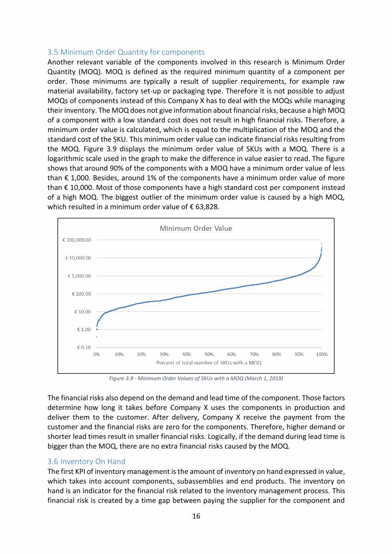
3.5 Minimum Order Quantity for components Another relevant variable of the components involved in this research is Minimum Order Quantity (MOQ). MOQ is defined as the required minimum quantity of a component per order. Those minimums are typically a result of supplier requirements, for example raw material availability, factory set-up or packaging type. Therefore it is not possible to adjust MOQs of components instead of this Company X has to deal with the MOQs while managing their inventory. The MOQ does not give information about financial risks, because a high MOQ of a component with a low standard cost does not result in high financial risks. Therefore, a minimum order value is calculated, which is equal to the multiplication of the MOQ and the standard cost of the SKU. This minimum order value can indicate financial risks resulting from the MOQ. Figure 3.9 displays the minimum order value of SKUs with a MOQ. There is a logarithmic scale used in the graph to make the difference in value easier to read. The figure shows that around 90% of the components with a MOQ have a minimum order value of less than € 1,000. Besides, around 1% of the components have a minimum order value of more than € 10,000. Most of those components have a high standard cost per component instead of a high MOQ. The biggest outlier of the minimum order value is caused by a high MOQ, which resulted in a minimum order value of € 63,828.

The financial risks also depend on the demand and lead time of the component. Those factors determine how long it takes before Company X uses the components in production and deliver them to the customer. After delivery, Company X receive the payment from the customer and the financial risks are zero for the components. Therefore, higher demand or shorter lead times result in smaller financial risks. Logically, if the demand during lead time is bigger than the MOQ, there are no extra financial risks caused by the MOQ.

3.6 Inventory On Hand The first KPI of inventory management is the amount of inventory on hand expressed in value, which takes into account components, subassemblies and end products. The inventory on hand is an indicator for the financial risk related to the inventory management process. This financial risk is created by a time gap between paying the supplier for the component and

Figure 3.9 - Minimum Order Values of SKUs with a MOQ (March 1, 2019)

17

receiving the payment of the customer for the product. In this research, the amount of inventory hold for Customer Y is only taken into account. Therefore, for every month in 2018 is the amount of inventory on hand for Customer Y determined. This value is dependent on the sales and operations planning of Company X, because increasing sales will result in a higher amount of inventory on hand. The inventory on hand has to be compared with the projected amount of inventory and the corporate goal of the amount of inventory. Figure 3.10 shows the development of the amount of inventory on hand per month through 2018. The graph shows that the inventory on hand decreased in the second part of the year. Next to this, the inventory on hand comes closer to or becomes even less than the inventory on hand projection in the last months of 2018. In general, companies always have the goal to reduce the amount of inventory on hand. Despite, this research focusses on reducing the cycle time for products for Customer Y. Therefore, an analysis of the amount of inventory on hand always have to take the performances of the company with respect to cycle time or sales into account.

3.7 Inventory turnover The second KPI related to inventory management at Company X is the inventory turnover of the total inventory on hand, which includes components, subassemblies and end products. The inventory turnover measures the number of times inventory turns over in a year. (Chopra & Meindl, 2013) It is the ratio of average inventory to either the cost of goods sold or sales. The cost of goods sold is relevant in this research, because the management of inventory of components is investigated. The following formula is used to calculate the inventory turns:

𝐼𝑛𝑣𝑒𝑛𝑡𝑜𝑟𝑦 𝑡𝑢𝑟𝑛𝑜𝑣𝑒𝑟 =𝐶𝑜𝑠𝑡 𝑜𝑓 𝑔𝑜𝑜𝑑𝑠 𝑠𝑜𝑙𝑑 𝑖𝑛 𝑚𝑜𝑛𝑡ℎ∗12

𝐴𝑣𝑒𝑟𝑎𝑔𝑒 𝑖𝑛𝑣𝑒𝑛𝑡𝑜𝑟𝑦 € ( 3.1 )

Inventory turnover can be a very useful measure, especially when comparing divisions of a firm or firms in an industry. (Silver, Pyke, & Thomas, 2017) Firms in different industries or with a different strategy can have different inventory turnovers due to a difference in for example Work In Progress. Therefore, strategic competitive advantage can have a significant effect on the determination of the appropriate inventory turnover number. (Silver, Pyke, & Thomas, 2017) The equation of the inventory turnover shows that an increase in sales without a

Figure 3.10 - Inventory On Hand in 2018

18

corresponding increase in inventory will increase the inventory turnover, as well a decrease in inventory without a decline in sales. During this research, the goal is to reduce the cycle time by applying efficient inventory management. Therefore, the objective is to have an appropriate inventory turnover instead of maximizing the inventory turnover, because otherwise the requested cycle time will not be achieved. The inventory turnover per month of Company X in 2018 is shown in Figure 3.11. The number have to be compared with the corporate goal, which is for the first eleven months 6.5. The figure shows that in most months the inventory turnover is lower than the goal of 6.5. There are three exceptions and two of them are in the last months of the year. The higher inventory turnover are mainly caused by a decrease in inventory on hand.

3.8 Causes of high lead times The previous sections describes the aspects and variables related to the cycle time of the products for Customer Y at Company X. This cycle time influence directly the committed lead time for the products with Customer Y. The Order Lead Time (OLT) is defined as the total time between confirming SO and delivering the order at the customer. A part of this lead time is used for assembling components to subassemblies and sequentially assembling the end products. In the past, Company X and Customer Y agreed about OLTs for the products and applied those lead times in their supply chain. Figure 3.12 shows the percentage of products with a specific lead time between 0 en 40 weeks. This confirms that not only the ICTs of Company X are high, but also the OLTs are high.

The above described analysis of the different aspects of the cycle time and lead time already showed which causes should be investigated in this research. Mainly the long lead times of components and relatively short internal assembly times of subassemblies and products showed the urgency of improving the inventory management of components. The lead times of components showed that reducing the cycle time and lead time is not achievable without having safety stocks or open orders at suppliers. Besides, the percentage of late deliveries of suppliers with impact on production confirmed that executing a research into the safety stocks is necessary. This can be beneficial for the cycle and lead time, but also reduce the disruptions in the planning and production departments.

Figure 3.11 - Inventory turnover in 2018

19

3.9 Conclusion This chapter describes an analysis of the current situation of inventory management at Company X. This analysis results in an answer to the first research question:

What is the current situation at Company X with respect to inventory policy and resulting cycle times?

First, it is important to understand which aspects determine the cycle times. Therefore, Section 3.1 describes which variables are relevant during this research. As mentioned earlier, the first part of the process consists of purchasing components at suppliers. Therefore, the current situation with respect to lead times of components and the reliability of those lead times are important for the inventory policy and resulting cycle times of products. Section 3.2 elaborates on the lead times of components and shows that those lead times are relatively long compared to the cycle time and lead time of products. Besides, this section shows that the supplier do not always deliver the components within the agreed lead time, which results in disruptions in the production and planning processes. The production processes consist of assembling subassemblies and sequentially assembling the product. Section 3.3 quantifies the internal assembly times of products and subassemblies. Those assembly times are relatively short compared to the lead time of components. Those first two sections confirm that the cycle times have to be reduced by applying the right inventory policies for components.

In Section 3.4 is described what the current situation is with respect to safety stocks. At Company X, safety stocks are only applied at component level. However, a large part of components does not have a safety stock. Besides, there is no clear explanation for the current safety stock and they are often not aligned with the demand and order quantities of the components. The order quantities have to be determined during this research given the MOQs of components, which are shortly discussed in Section 3.5. In the case of the components relevant for this research, most of the MOQs do not result in extreme order values.

Figure 3.12 - Histogram of lead times products

20

Another important aspect of inventory management is the financial side of having inventory. Section 3.6 discusses the historical amount of inventory on hand for Customer Y and compares this with the projection and goal. The research has to take the amount of inventory into account when optimizing the inventory management. And Section 3.7 shows that the inventory turnover of Company X is in general lower than the corporate goal, which also confirms the need for an improved inventory policy.

Section 3.7 relates the different aspects of cycle and lead time with the current lead times. This section shows that the inventory management of Company X should be investigated. In the upcoming chapter, there is literature related to inventory management presented. The literature study focusses on inventory policies, item classification, calculating safety stock and reorder points, because this chapter confirmed that with the current management of inventory is it not possible to reduce the cycle time and lead time. The analysis of this literature has to give insights in how inventory management can be applied to reduce cycle times and lead times at Company X. Thereafter, there is a model constructed to determine which inventory policy should be applied. This model has to take financial risk into account. Besides, the input of the model has to be configurable and generic to make it possible to implement it at Company X over a longer time horizon.

21

4 Literature review Now the problem and current situation of Company X are clear, this chapter will present relevant inventory management concepts and link them to the situation within Company X. The inventory management concepts are retrieved from existing literature. The importance of inventory management and the relevant types of inventory are described in Section 4.1. Thereafter, Section 4.2 elaborates on different inventory control policies and their advantages and disadvantages. Thereafter, Section 4.3 gives insights in classification methods, which can be applied to select different inventory policy per class. In the following three sections is theory about the Economic Order Quantity (EOQ), reorder point and safety stock presented. These sections will also present the corresponding formulas. In Section 4.7 is presented how the literature can be applied in the research’s context. This chapter will be closed by a conclusion in Section 4.8 with an answer to the following research question:

What methods are suggested in the literature to achieve smaller cycle times considering the inventory policy?

4.1 Inventory management The strategic benefits of inventory management have become obvious since the mid-1980s. Nowadays many firms coordinate with other firms in their supply chains. Instead of responding to unknown and highly variable demand, companies in the supply chain share information so that the variability of the demand they observe is significantly lower (Silver, Pyke, & Thomas, 2017). The objective of a company is having an effective and efficient inventory control. Companies try to reduce inventories to decrease the costs of inventory. Nevertheless, there are limits on reducing inventories, because companies cannot perform at a competitive level without inventories. The most important and relevant reasons for having inventories are:

- Economies of scale - Shortening cycle times to the customers - Buffering against uncertainties in supply and/or demand

4.1.1 Functional classification of inventories The term inventory does not clearly specify the function of the involved inventory. For this reason, Silver, Pyke, and Thomas (2017) provide functional classifications of inventories. The following classification of inventory types is made:

- Cycle inventories: inventories resulting from ordering or producing batches.

- Congestion stocks: inventories due to items competing for limited capacity. - Safety stocks: inventories to anticipate on uncertainty of demand and

the uncertainty of supply. - Anticipation inventories: stock accumulated in advance of an expected peak in

sales. - Pipeline inventories: goods in transit between levels of a multi-echelon

distribution system or between adjacent workstations in a factory.

- Decoupling stocks: inventories used in a multi-echelon situation to permit the separation of decision making at the different echelons.

22

4.1.2 Cycle and safety inventory In this research, the cycle inventories and safety stocks are investigated and the other types of inventory are not relevant for the situation of Company X. As mentioned above, cycle inventory is caused by ordering or producing batches. Chopra and Meindl (2013) do have a similar definition as Silver, Pyke and Thomas (2017), namely cycle inventory is the average inventory in a supply chain due to either production or purchases in lot sizes that are larger than those demanded by the customer. The reasons for larger lot sizes include economies of scale, quantity discounts in purchase price or freight cost, and technological restrictions. This results in a trade-off between ordering and freight costs and inventory costs for a company. The frequency of orders directly influences the amount of cycle stock on hand at any time. Less frequently ordering results in larger order sizes, which results in a higher cycle inventory. Figure 4.1 shows the relationship between order size (Q) and cycle inventory given deterministic and constant demand.

Safety stock is the amount of inventory kept on hand to allow for the uncertainty of demand and the uncertainty of supply in the short run (Silver, Pyke, & Thomas, 2017). Therefore, safety stocks are not needed when the future demand and the length of time it takes to get complete delivery of an order are known with certainty. The level of safety stock is directly related to the desired level of customer service. This results in a tradeoff between holding costs and customer service level. Desiring a higher level of customer service results in a higher level of safety stock, which increases the holding costs. The influence of safety stock on the inventory profile is displayed in Figure 4.1. Higher safety stock results in higher inventory levels and a higher average inventory, which means that the financial investment will be higher. Important to note is that Figure 4.1 shows an inventory profile with a deterministic and constant demand. However, in this research annual demand will be modelled as deterministic demand, but there are fluctuations in the weekly demand. Despite, the definition of cycle and safety inventory is the same in both cases.

Figure 4.1 - Inventory profile with cycle and safety inventory (Kim)

23

4.2 Inventory control policies Another aspect of inventory management is the type of inventory control policy. The inventory control policy is dependent on how often the inventory status should be determined. This determines the review interval (R), which is the time that elapses between two consecutive moments at which we know the stock level (Silver, Pyke, & Thomas, 2017). There are two possibilities of review, namely continuous review and periodic review. In the first case, the stock status is always known by immediately updating the stock status after each transaction (shipment, receipt, demand, etc.). With periodic review, the stock status is determined every R time units. During this review period may be uncertainty considered in the stock level. Therefore, the major advantage of continuous review is that, to provide the same level of customer service, it requires less safety stock compared to periodic review. The period over which safety protection is required is longer under periodic review. This results in the opportunity for the stock level to drop between review instants without any reordering action.

After distinguishing a continuous or periodic review, there have to be specified which form of inventory control policy is used. The form of the inventory policy determines when an order should be placed and what quantity should be ordered (Silver, Pyke, & Thomas, 2017). The different policies with their characteristics with respect to order quantity and review period are shown in Table 4.1. In these policies, s is the reorder point, Q is the order quantity, S is the order-up-to-level and R is the review period.

Table 4.1 - Inventory control policies

Continuous review Periodic review

Fixed order quantity (s,Q) (R,s,Q)

Variable order quantity (s,S) (R,S) or (R,s,S)

4.2.1 Continuous review policies

(s,Q) policy This system is continuously reviewed and a fixed order quantity Q is ordered when the inventory position drops to or lower than the reorder point s. An important side note is that the inventory position is used to trigger an order and not the net stock. Otherwise, the on-order stock will not be taken into account and this can result in placing unnecessarily orders. The (s,Q) system is often called a two-bin system. The first bin satisfies the demand, as long as there are units in the first bin. The amount of units in the second bin corresponds to the reorder point. As soon as the first bin is empty, the second bin is opened and a replenishment order is placed. When the replenishment order arrives, first the second bin is filled and the remaining units is put into the first bin. The advantages of using this fixed order-quantity system include that it is quite simple, that errors are less likely to occur and that the required production of the supplier is quite predictable (Silver, Pyke, & Thomas, 2017). Figure 4.2 displays a numerical example of the (s,Q) policy.

24

(s,S) policy

The (s,S) system again assumes continuously reviewing the inventory position and a replenishment order is placed whenever the inventory position drops to the reorder point s or lower. The difference with the (s,Q) system is that a variable replenishment quantity is used. This quantity is determined by ordering enough to raise the inventory position to the order-up-to-level S. In the case of unit sized demand transactions, the two systems are identical because a replenishment order will always be placed when the inventory position is equal to s and the order-up-to-level will be S = s + Q. Once the demand transactions are larger than unit size, the quantity of the replenishment order becomes variable. The (s,S) policy is frequently referred to a min-max system, because the inventory position is almost always between a minimum value of s and a maximum value of S. The inventory position can only drop below the minimum in the case of a temporary fall below the reorder point. The advantage of finding the best (s,S) policy in comparison with the best (s,Q) policy is lower total costs of replenishment, carrying inventory and shortage. However, finding the best (s,S) policy requires a substantially greater computational effort. Therefore, the potential savings of calculating the best (s,S) policy need to be significant. The disadvantage of the (s,S) policy is the variable order quantity, which reduce predictability for the supplier and therefore could increase the frequency of errors in delivering the right quantity at the right time. A numerical example of a (s,S) policy is shown in Figure 4.3 - (s,S) policy .

Figure 4.3 - (s,S) policy (Silver, Pyke, & Thomas, 2017)

Figure 4.2 - (s,Q) policy (Silver, Pyke, & Thomas, 2017)

25

4.2.2 Periodic review policies

(R,s,Q) policy The (R,s,Q) policy only reviews the inventory position every interval period R. If the inventory level is equal or lower than the reorder point s, then a replenishment order of a fixed quantity Q is placed. This Q has to be high enough to get the inventory position above the reorder point s (Kuncoro, Aurachman, & Santosa, 2018). A disadvantage of this policy is the fixed order quantity Q, because during the interval period R is demand uncertain. This makes it difficult to determine an acceptable Q for a component with uncertainties in demand during the review period. This policy is therefore only reliable for components with a constant demand.

(R,S) policy The (R,S) policy is also known as a replenishment cycle system, because every R units of time is the inventory position raised to the order-up-to-level S. This system is in common use in companies without sophisticated computer systems to continuously adapt and monitor the inventory positions. An advantage of the (R,S) policy is the regular opportunity to adjust the order-up-to-level S, if the demand pattern is changing with time. Despite, disadvantages of the (R,S) system are the variable replenishment quantities and the higher carrying costs compared to the continuous review systems (Silver, Pyke, & Thomas, 2017). Figure 4.4 shows an example of a (R,S) policy with R is 10 weeks and a lead time of 2 weeks.

(R,s,S) policy The last policy is a combination of the (s,S) and (R,S) policy, namely the (R,s,S) policy. The inventory position is checked every R units of time. If the inventory position is at or lower than the reorder point s, there is a replenishment order placed to raise the inventory position to the order-up-to-level S. Otherwise, if the inventory position is above s, there is nothing done until the next review moment. The (s,S) policy is a special case of the (R,s,S) policy where R is zero. The (R,S) policy is also a special case of the (R,s,S) policy where s is equal to S-1. The best (R,s,S) systems result in lower replenishment, carrying and shortage costs than the other systems. However, there is more computational effort required to obtain the values of the three parameters. Therefore, the trade-off between computational effort and potential savings have to be made before selecting this policy (Silver, Pyke, & Thomas, 2017).

Figure 4.4 - (R,S) policy (Silver, Pyke, & Thomas, 2017)

26

4.3 Item classification Decision regarding inventory management should be made at the level of an individual item or product. A specific unit of stock to be controlled is called a stock-keeping unit (SKU). A SKU is defined as an item of stock that is specified with respect to function, style, size, color and location. Production companies generally have to deal with hundreds or even thousands of SKUs. Differences in SKU-characteristics can result in different production and inventory policies (Van Kampen, Akkerman, & van Donk, 2012). Companies with a wide variety of SKUs often struggle with the control of their production and inventory systems. For this reason, classifying SKUs provides companies guidance in decision making for entire SKU classes instead of each SKU separately.

4.3.1 ABC analysis There are several SKU-classification methodologies established through the years. One of the most well-known methodologies is the ABC analysis. This methodology classifies SKUs based on dollar volume. It is very common that a relatively small percentage of the SKUs account for a large share of the total volume. Typically twenty percent of the SKUs accounts for about eighty percent of the dollar volume. Therefore, the SKUs with a high contribution to the dollar volume are often more important, and this makes it reasonable to put more effort in the inventory control and evaluation of those SKUs (Axsäter, 2015). Based on the Distribution by Value (DBV) of SKUs can be decided to which extent the inventory of the SKUs should be controlled. A DBV curve can be developed by identifying the value in dollars per unit and the annual demand of each SKU. Thereafter, the product of the value in dollars and demand is taken, and ranked in descending order starting with the largest value (Silver, Pyke, & Thomas, 2017). Then the values of the cumulative percent of total dollar usage and the cumulative percent of the total number of SKUs in inventory are plotted on a graph such as Figure 4.5 - Distribution by Value of SKUs . This confirms that approximately 20% of the SKUs contribute to 80% of the DBV. The SKUs with the highest contribution to the DBV, should get a higher priority assigned with respect to allocation of management time and financial resources. In general, three priority ratings are made: A (most important), B (intermediate in importance), and C (least important).

Figure 4.5 - Distribution by Value of SKUs (Silver, Pyke, & Thomas, 2017)

27

4.3.2 Multi-criteria ABC analysis The ABC analysis is famed for its ease of use, but it has been criticized for its exclusive focus on dollar usage. Other criteria such as lead-time, commonality, obsolescence, durability, inventory cost, and order size requirements have also been recognized as critical for inventory classification (Yu, 2011). Therefore, classifying items based on value and demand is not always optimal for an organization. Through the years, there are developed two main approaches to classify items based on multiple criteria, namely the joint criteria matrix and the Analytic Hierarchy Process (AHP).

The first approach is the joint criteria matrix, which considers two criteria for classification. The matrix consists of nine different cells, which has the consequence that a two criteria joint matrix may require nine different policies to deal with inventory items. Implementing and managing nine different policies would be difficult. Therefore a reclassification of items into an appropriate number of categories is often done (Flores & Whybark, 1986).

Secondly, the Analytic Hierarchy Process (AHP) is the second approach, which is based on the experience gained by its developer T.L. Saaty. The decisions with respect to generate priorities in an organized way are decomposed into the following steps (Saaty, 2008):

1) Define the problem and determine the type of knowledge needed. 2) Structure the decision hierarchy from the top level with the objective of the decision, then

continue to objectives from a broad perspective, through the intermediate levels to the lowest level.

3) Construct pairwise comparison matrices, where each element in an upper level is compared with elements in the level immediately below.

4) Use the priorities obtained from the comparison to weigh the priorities in the level immediately below. Execute this for every element. Then for each element in the level below add its weighed values and obtain its overall priority. Continue with this step of weighing and adding until the final priorities in the lowest level are obtained.

AHP generates a consistent measure for classifying items and the assignment of items of classes is more uniform and the quality and completeness of the inventory analysis. Disadvantages of AHP are the managerial time needed to develop the needed information for each item and the subjectivity involved in the analysis.

4.3.3 XYZ-analysis The last method for classifying components is the XYZ-analysis. During this analysis is the predictability of items evaluated. The prediction accuracy is determined by the coefficient of variation (CV), which is a relative measure of variation (Stoll, Kopf, Schneider, & Lanza, 2015). The standard deviation indicates the variation, but the relative measure depends on the corresponding mean. Therefore, the coefficient of variation is calculated by dividing the standard deviation by the mean, which results in the following formula:

𝐶𝑜𝑒𝑓𝑓𝑖𝑐𝑖𝑒𝑛𝑡 𝑜𝑓 𝑣𝑎𝑟𝑖𝑎𝑡𝑖𝑜𝑛 (𝐶𝑉) = 𝜎

𝜇 ( 4.1 )

The standard deviation and mean have to be determined per item. The standard deviation can include demand variation, supply variation or even a combination of both. Therefore, it is important to know what kind of predictability is included while using the XYZ analysis. After calculating the CVs of the items, the items can be divided into the different categories. The XYZ limits are determined in collaboration with experts (Stoll, Kopf, Schneider, & Lanza, 2015).

28

The description and limits of the categories are shown in Table 4.2. The items of different categories may need different inventory policies. For items in category X is a fixed order quantity applicable, because the variation is predictable. Despite, items in category Z may require a manual inventory control with order sizes based on received demand, because the variation in demand is random.

Table 4.2 - XYZ-analysis categories

Category Description Limits

X Uniform, constant course of demand CV < 1.5

Y Average prediction accuracy 1.5 ≤ CV < 3

Z Random course of demand CV > 3

4.4 Economic Order Quantity (EOQ) There is a direct relation between the cycle inventory and order quantities of a product. There have to be three different types of annual costs considered when finding the optimal order quantity, namely material cost, order cost and holding cost. The annual material costs depends on the purchase price and the annual demand. The annual order costs depends on the order costs and the number of orders placed per year, which is dependent on the annual demand and the lot size. Lastly, the annual holding costs are determined by the average inventory and holdings cost of a product. This holding cost of a product can be calculated with the cost of the product and the holding costs per year as fraction of the product cost. With those cost components are the total annual cost per year calculated with the following formula (Chopra & Meindl, 2013):

𝑇𝑜𝑡𝑎𝑙 𝑎𝑛𝑛𝑢𝑎𝑙 𝑐𝑜𝑠𝑡 = 𝑀𝑎𝑡𝑒𝑟𝑖𝑎𝑙 𝑐𝑜𝑠𝑡 + 𝑂𝑟𝑑𝑒𝑟𝑖𝑛𝑔 𝑐𝑜𝑠𝑡 + 𝐻𝑜𝑙𝑑𝑖𝑛𝑔 𝑐𝑜𝑠𝑡

𝑇𝐶 = 𝐶 ∗ 𝐷 + (𝐷

𝑄) ∗ 𝑆 + (

𝑄

2) ∗ ℎ ∗ 𝐶 ( 4.2 )

𝐶 = 𝐶𝑜𝑠𝑡 𝑝𝑒𝑟 𝑢𝑛𝑖𝑡 𝐷 = 𝐴𝑛𝑛𝑢𝑎𝑙 𝑑𝑒𝑚𝑎𝑛𝑑 𝑜𝑓 𝑡ℎ𝑒 𝑝𝑟𝑜𝑑𝑢𝑐𝑡 𝑄 = 𝑂𝑟𝑑𝑒𝑟𝑖𝑛𝑔 𝑞𝑢𝑎𝑛𝑡𝑖𝑡𝑦 𝑆 = 𝐹𝑖𝑥𝑒𝑑 𝑐𝑜𝑠𝑡 𝑖𝑛𝑐𝑢𝑟𝑟𝑒𝑑 𝑝𝑒𝑟 𝑜𝑟𝑑𝑒𝑟 ℎ = 𝐻𝑜𝑙𝑑𝑖𝑛𝑔 𝑐𝑜𝑠𝑡 𝑝𝑒𝑟 𝑦𝑒𝑎𝑟 𝑎𝑠 𝑓𝑟𝑎𝑐𝑡𝑖𝑜𝑛 𝑜𝑓 𝑝𝑟𝑜𝑑𝑢𝑐𝑡 𝑐𝑜𝑠𝑡

The optimal order quantity is the one that minimizes the total cost. This is obtained by taking the first derivative of the total cost with respect to Q and setting it equal to 0. The optimal order quantity is called the Economic Order Quantity (EOQ). The formula to determine the EOQ of a product is (Silver, Pyke, & Thomas, 2017):

𝐸𝑂𝑄 = √2∗𝐷∗𝑆

ℎ∗𝐶 ( 4.3 )

There need to be made assumption before the above mentioned EOQ can be calculated. Some of these assumptions are quite strong and may be quite limiting, but Zheng (1992) has shown that the fractional cost penalty of using the EOQ instead of a more complex calculation is not that significant. In other words, the extra complexity and computational time needed does not weigh up to the benefits. The following assumptions have to be made to determine the basic EOQ (Silver, Pyke, & Thomas, 2017):

29

1) The demand rate is constant and deterministic. 2) The order quantity does not need to be an integer. 3) The cost per unit does not depend on the order quantity. 4) The cost factors do not change appreciably with time. 5) The item is treated entirely independently of other items. 6) The replenishment lead time is deterministic. 7) No shortages are allowed. 8) The entire order quantity is delivered at the same time. 9) The planning horizon is pretty long, which means parameters keep constant.

As mentioned earlier, some of these assumptions are more strict than others. Therefore, it is often possible to first calculate the EOQ given these assumptions. Thereafter, by relaxing the assumptions, the optimal order quantity can be adjusted to the real life situation for the item.

4.5 Reorder point Managing inventory has the goal to prevent stock outs of components, which would disrupt the production planning and eventually increase the cycle time. Section 4.1.2 elaborates on how the Economic Order Quantity is determined. The EOQ considers constant demand and does not consider uncertainties in the inventory management process. Next to the quantity of an order, the decision about when an order should be placed is part of inventory management. An order should be placed early enough so that the expected demand during lead time does not exceed the inventory level at the moment of placing the order. Lead time is defined as the time that expires from the moment at which is decided to place an order, until it is stored physically on the shelf and ready to satisfy demand (Silver, Pyke, & Thomas, 2017).

When the demand and lead time of an item are known, the exact time to place an order can be calculated. In that case there is no excess stock or unsatisfied demand. This is called defining the reorder point, which reflects the level of inventory that triggers the placement of an order for additional units (Chen, 1998). However, in practice there might be some variation in the demand and the lead time. Therefore, it is useful for a company to consider safety stocks. Safety stock is the amount of inventory of a component held in case demand exceeds expectations; it is held to counter uncertainty (Chopra & Meindl, 2013).

Concluding there are three factors related to the reorder point of an item, namely the demand per time unit (D), lead time (LT) and the safety stock (SS). The relation between the reorder point, lead time and order quantity is shown in Figure 4.6. The figure shows how the stock level behaves over time given a continuous review policy. The reorder point is determined based on the lead time and demand, which result in orders arriving when the stock level is equal to zero.

30

As the figure shows, if demand is constant and lead time is known, there is no safety stock needed for an item. Then the reorder point needs to be exactly high enough to cover the demand during lead time. Therefore, the formula for the reorder point is as follows (Waters, 2003):

𝑅𝑒𝑜𝑟𝑑𝑒𝑟 𝑝𝑜𝑖𝑛𝑡 = 𝑙𝑒𝑎𝑑 𝑡𝑖𝑚𝑒 ∗ 𝑑𝑒𝑚𝑎𝑛𝑑 𝑝𝑒𝑟 𝑡𝑖𝑚𝑒 𝑢𝑛𝑖𝑡 = 𝐿𝑇 ∗ 𝐷 ( 4.4 )

Despite, it is almost never the case that demand and lead time is constant and known. Therefore, there is kept safety stock for an item, which results in the following calculation for the reorder point (Waters, 2003):

𝑅𝑒𝑜𝑟𝑑𝑒𝑟 𝑝𝑜𝑖𝑛𝑡 = (𝑙𝑒𝑎𝑑 𝑡𝑖𝑚𝑒 ∗ 𝑑𝑒𝑚𝑎𝑛𝑑 𝑝𝑒𝑟 𝑡𝑖𝑚𝑒 𝑢𝑛𝑖𝑡) + 𝑠𝑎𝑓𝑒𝑡𝑦 𝑠𝑡𝑜𝑐𝑘 𝑅𝑒𝑜𝑟𝑑𝑒𝑟 𝑝𝑜𝑖𝑛𝑡 = 𝐿𝑇 ∗ 𝐷 + 𝑆𝑆 ( 4.5 )

The formula above does not show which variables should be selected to calculate the reorder point. Therefore, the following formula has to be used to calculate the reorder point in case of variability in demand and supply (Hopp & Spearman, 2008):

𝑅𝑒𝑜𝑟𝑑𝑒𝑟 𝑝𝑜𝑖𝑛𝑡 = 𝐿𝑇 ∗ 𝜇𝐷 + 𝑆𝑆 ( 4.6 )

Because of uncertainty in demand and supply, the D is replaced by 𝜇𝐷, which is the average demand per time unit. Next to this, the calculation of the safety stock depends on the fill rate and the 𝜎 of demand and supply. Section 4.6 elaborates on the calculation of those variables and the resulting safety stock.

4.6 Safety stock Obviously, it is very important to calculate the safety stock with an accurate and effective method. There are various methods established through the years with different assumption with respect to variability in demand and variability in lead time. An important assumption in this section is that if there is variability in demand and/or lead time, then the demand and/or lead times are normally distributed. In this research related to the case of Company X, only variation in demand is considered in determining the safety stock. This is because there is no data available for variation in supply and this is too unpredictable that it is not possible to quantify the variation in supply. This is partly caused by the industry, because of allocation parts with a very long and variable lead time.

Figure 4.6 - Reorder point, lead time and order quantity (modified from (Waters, 2003))

31

The first step in determining an appropriate level of safety inventory is measuring product availability. There are three main measurement known in the literature, namely product fill rate, order fill rate and cycle service level. The goal of this research is increasing availability of components to production, which has to reduce the cycle time. Therefore, it makes sense to apply the product fill rate as availability measurement, because it measures the fraction of demand that is satisfied from inventory. The order fill rate measures the fraction of orders that are filled and the cycle service level measures the fraction of replenishment cycles that end with all the demand being met. (Chopra & Meindl, 2013) The last two do not quantify the number of components involved in an order or replenishment cycle.

After measuring the product availability, the variability in demand has to be measured and quantified. As mentioned above, the assumption is often made that demand is normally distributed and for this reason the standard deviation is used to measure the demand. In this research, the standard deviation of demand per week is measured with the following formula: (Chopra & Meindl, 2013)

𝑆𝑡𝑎𝑛𝑑𝑎𝑟𝑑 𝑑𝑒𝑣𝑖𝑎𝑡𝑖𝑜𝑛 𝑝𝑒𝑟 𝑤𝑒𝑒𝑘 (𝜎) = √1

𝑁∗ ∑ (𝑥𝑖 − 𝜇)2𝑁

𝑖=1 ( 4.7 )

𝑥𝑖 = 𝑑𝑒𝑚𝑎𝑛𝑑 𝑖𝑛 𝑤𝑒𝑒𝑘 𝑖 𝜇 = 𝑎𝑣𝑒𝑟𝑎𝑔𝑒 𝑑𝑒𝑚𝑎𝑛𝑑 𝑝𝑒𝑟 𝑤𝑒𝑒𝑘 𝑁 = 𝑡𝑜𝑡𝑎𝑙 𝑛𝑢𝑚𝑏𝑒𝑟 𝑤𝑒𝑒𝑘𝑠 𝑤𝑖𝑡ℎ 𝑑𝑒𝑚𝑎𝑛𝑑 𝑑𝑎𝑡𝑎

The standard deviation per week can be easily translate to the standard deviation during the period of demand uncertainty. This can be done by multiplying the standard deviation with the square root of the period in weeks, which results in this formula:

𝑆𝑡𝑎𝑛𝑑𝑎𝑟𝑑 𝑑𝑒𝑣𝑖𝑎𝑡𝑖𝑜𝑛 𝑑𝑢𝑟𝑖𝑛𝑔 𝑝𝑒𝑟𝑖𝑜𝑑 (𝜎) = 𝜎 ∗ √𝑝𝑒𝑟𝑖𝑜𝑑 𝑖𝑛 𝑤𝑒𝑒𝑘𝑠 ( 4.8 )

The next step is calculating the Expected Shortage per replenishment Cycle (ESC). This variable is calculated based on the desired fill rate and determined order quantity, as described earlier. This ESC is used to calculate the required safety stock to obtain the desired fill rate. The following formula is used to calculate the ESC (Chopra & Meindl, 2013):

𝐸𝑆𝐶 = (1 − 𝑓𝑟) ∗ 𝑄 ( 4.9 ) 𝑓𝑟 = 𝑓𝑖𝑙𝑙 𝑟𝑎𝑡𝑒 𝑄 = 𝑜𝑟𝑑𝑒𝑟 𝑞𝑢𝑎𝑛𝑡𝑖𝑡𝑦

Now, the safety stock can be determined given the ESC and the standard deviation. The safety stock sizes are determined based on a desired fill rate and the standard deviation of demand. The formula above calculates the ESC based on fill rate and order quantity. The formula beneath calculates the ESC based on safety stocks and standard deviation of demand:

𝐸𝑆𝐶 = −𝑠𝑠 ∗ [1 − 𝐹𝑠 (𝑠𝑠

𝜎)] + 𝜎 ∗ 𝑓𝑠 (

𝑠𝑠

𝜎) ( 4.10 )

𝑠𝑠 = 𝑠𝑎𝑓𝑒𝑡𝑦 𝑠𝑡𝑜𝑐𝑘 𝑠𝑖𝑧𝑒 𝜎 = 𝑠𝑡𝑎𝑛𝑑𝑎𝑟𝑑 𝑑𝑒𝑣𝑖𝑎𝑡𝑖𝑜𝑛 𝑑𝑢𝑟𝑖𝑛𝑔 𝑔𝑎𝑝 𝐹𝑠(… ) = 𝑠𝑡𝑎𝑛𝑑𝑎𝑟𝑑 𝑛𝑜𝑟𝑚𝑎𝑙 𝑐𝑢𝑚𝑢𝑙𝑎𝑡𝑖𝑣𝑒 𝑑𝑖𝑠𝑡𝑟𝑖𝑏𝑢𝑡𝑖𝑜𝑛 𝑓𝑢𝑛𝑐𝑡𝑖𝑜𝑛 𝑓𝑠(… ) = 𝑠𝑡𝑎𝑛𝑑𝑎𝑟𝑑 𝑛𝑜𝑟𝑚𝑎𝑙 𝑑𝑒𝑛𝑠𝑖𝑡𝑦 𝑓𝑢𝑛𝑐𝑡𝑖𝑜𝑛

32

To determine the safety stock size, both formulas should result in the same value for the ESC. The Excel tool Goalseek can be used to determine the required safety stock size. (Chopra & Meindl, 2013)

The above mentioned formulas for calculating reorder point and safety stock are applicable to the continuous review policy. If a periodic review policy is used, the variable lead time (LT) has to be replaced for lead time plus review period (LT+R). Therefore, depending on which inventory control policy is selected for an item, the right formulas have to be selected to calculate the reorder point and safety stock.

4.7 Application of literature in the research’s context The above described methods found in the literature are of course not directly applicable in the context of this research without making any assumptions. The application of cycle and safety inventory is already justified in Section 4.1. The other types of inventory are not used in the process of Company X.

4.7.1 Inventory policy In Section 4.2, the different inventory control policies are extensively described. In the current situation of Company X, an ERP-system (Baan) is used to manage the inventory of items. Therefore, a continuous review policy can be applied, because the ERP-system monitors the inventory position based on production, purchase orders and planned deliveries. This ERP-system uses some specific input parameters with respect to inventory management. Figure 4.7 shows the options of the ERP-system with respect to the implementation of the parameters for an ordering policy. First, the order method is selected, which has four options:

- Lot for lot - Economic Order Quantity - Fixed Order Quantity - Replenish to maximum inventory

The order method of using the Economic Order Quantity can be used for applying a fixed order quantity in the case of applying the (s,Q) policy. And in the case of applying the (s,S) policy, the replenish to maximum inventory can be selected by setting the maximum inventory equal to the order-up-to-level.

33

Next to the order method, the order quantity settings have to be specified, which are shown in Figure 4.7. The first parameter makes sure that there is always a multiple of a specific number ordered. This is often the case if the supplier of an item deliver them in specific packages with more than one item per package. Secondly, the minimum order quantity can be specified, which is a result of a restriction of suppliers. This is the same for the maximum order quantity, which can be caused by limitations in production of the supplier or a specific allocation of their products to their customers. The fourth parameter is the fixed order quantity, which could be used if the supplier has one specific order size of the item. Lastly, the Economic Order Quantity has to be specified. This parameter can be calculated with the formula presented in Section 4.4.

4.7.2 EOQ and safety stock determination There are formulas presented in Section 4.4 and Section 4.6 to calculate the EOQ and safety stock for an item. As mentioned in those sections, there need to be made some assumption to use these formulas. In Section 4.4, there are nine assumptions mentioned for calculating the EOQ. Logically, the context of this research do not completely match with the assumptions mentioned, which is often the case with company data. However, the formula provides a good estimation of an optimal quantity. Besides, the model will calculate EOQs and analyzing these values will show if there need to be made adjustments.

Next to this, the calculation of safety stock is done with parameters based on a service factor, demand and lead time of an item. There are three different formulas to take demand variability, lead time variability or both into account. In the case of Company X, lead time variability can be captured by adding safety lead time in the system for specific items. Therefore, the application of the formula for safety stock that considers demand variability fits to the context of this research.

Figure 4.7 - Item ordering parameters in the ERP-system

34

4.8 Conclusion This chapter presents a review of literature related to inventory management. The review results in an answer to the second research question:

What methods are suggested in the literature to achieve smaller cycle times considering the inventory policy?

First, the importance of inventory management is shortly described to verify if it is applicable to shorten cycle times. Then, Section 4.1 presents the importance and classifications of literature. After classifying inventory, the decision is made that for this research is cycle and safety inventory relevant and further investigated.

Thereafter, Section 4.2 elaborates on the different inventory control policies which are used to get more control of the inventory position over time. There is made a distinction between continuous and periodic review policies, which results in the following five policies:

- (s,Q) policy: continuous review with reorder point s and order quantity Q - (s,S) policy: continuous review with reorder point s and order-up-to-level S - (R,s,Q) policy: periodic review with review interval R, reorder point s and order

quantity Q - (R,s,S) policy: periodic review with review interval R, reorder point s and order-up-

to-level S - (R,S) policy: periodic review with review interval R, order-up-to-level S

To select an appropriate inventory control policy for items and reduce managerial effort, the involved items can be classified in different classes. Items can be classified based on several criteria, such as value, variation in demand, lead time etcetera. The classification methods found in the literature are the ABC analysis, joint criteria matrix, Analytic Hierarchy Process and the XYZ analysis, which are described in Section 4.3.

After selecting the right policy, the involved parameters have to be determined. Therefore, the well known Economic Order Quantity is used to find the optimal order quantity. Section 4.4 elaborates on the EOQ and describes the relation with the total holding and order costs. The other parameter of the inventory control policy is the reorder point. Section 4.5 describes the relation of the reorder point to demand, lead time and order quantity. Because of uncertainties in the process, the reorder point can be raised with adding safety stock for an item. Section 4.6 describes different formulas to calculate the safety stock given different situation with respect to demand and lead time variability.

The above described theory is used in the following chapters to model the inventory management process of Company X. By modelling the inventory management process, the optimal order quantities and safety stocks have to be determined given restrictions related to Company X’s process, which is already discussed in Section 4.7. The model has to give insights in resulting costs, risks and performances by changing their inventory management.

35

5 Model construction This chapter describes the constructed model and the resulting output from the model. The first step of creating a model is designing a conceptual model. This conceptual model presents which input data is needed to execute the calculations in the model and receive the output data. Section 5.1 presents the conceptual model and includes a visualization of the conceptual model. Thereafter, required input data and the connection to the model and resulting output data is explained. In Section 5.2 is the constructed model to determine the inventory policy parameters described and are calculations in the model presented and explained. In Section 5.3, the inventory policy parameters are used to calculate the output data of the model. This output is used to measure the performances resulting from selected inventory policies. The performance measurement of the model is used in the analysis in the next chapter. Lastly, Section 5.4 presents a conclusion and overview of this chapter.

5.1 Conceptual model The goal of this research and the constructed model is reducing the ICT of products by optimizing the inventory policy of the underlying SKUs. Therefore, the model should determine the inventory policies for the SKUs based on input data. Figure 5.1 gives an overview of the conceptual model. The figure distinguishes the data into three categories, namely input data, model data and output data. The arrows in the figure show how the data is connected to calculate the output data.

Figure 5.1 - Overview of the model

36

The input data consists of data and parameters. The required input data is data of the demand, the SKU characteristics and the products characteristics. In this section and in the model is the abbreviation SKU used for components. This data is extracted from the ERP-system and therefore this input data is dependent on the actual data in the system. Next to this, there are parameters related to inventory management and the model, namely order costs and holding cost rate. The values of these parameters are determined for Company X during this research. Besides, to execute the calculations in the model, the products need to have an obtained ICT and OLT. The obtained ICTs and OLTs are variable inputs and influences the model data and output data. Lastly, the model has a fill rate goal as variable input parameter, which influence the safety stocks and reorder points of the model.

The above described input data is used in the model to calculate for every SKU the order quantity, safety stock and reorder point. Then the model has to calculate the output resulting from the inventory policies of the SKUs. This output has to measure the inventory value, annual costs, financial risks and performances resulting from the ICT and OLT input and inventory policies. The output is used to analyze different scenarios and determine appropriate ICTs for the products based on the above mentioned measurements.

5.1.1 Input In the previous section, the required input data is presented in the overview of the conceptual model. The definitions given in the previous section are shortly described in this section. The relationship between the model data and output data will be explained. The following input data is needed in the model:

Input data from the ERP-system - SKU demand: The demand data of every involved SKU is needed to determine the

annual demand and variation of demand per week. The annual demand is used for order quantity calculation for SKUs. The variation of demand per week is used to calculate the required safety stock size for the SKU.

- Product demand: The product demand is the direct source of the SKU demand data, because the product demand and the BOM of the products determine the SKU demand. Next to this, for every involved product is the demand data needed to calculate the performance measurements. The demand data is used to calculate the ICT reduction, OLT reduction and financial consequences.

- SKU characteristics: For every involved SKU, there is information needed of the standard cost, Minimum Order Quantity, Multiple Order Quantity and lead time given by the supplier. This data is used to calculate the optimal order quantities and safety stocks.

- Product characteristics: The characteristics of products are also important input data. The current ICT, OLT and sales order price are needed to determine the ICT reduction, OLT reduction and financial consequences. Next to this, the MCT of the products are needed in the model to determine when SKUs need to be ordered.

Parameters determined during the research - Order cost: This parameter indicates the costs of placing and processing a purchase

order at a supplier by Company X. This parameters is used to determine the order quantities of the SKUs.

- Holding costs rate: This rate is used to calculate the holding costs of SKUs by multiplying the value of the components with this specific holding costs rate. Besides,

37

the holding cost rate is used in the calculation to determine the order quantities for the SKUs.

Variable input - ICT and OLT input: The ICT and OLT are both variable inputs in the model. The input

value will influence the outcome of all performance measurements. Company X and the customer have to agree about ICTs and OLTs for the involved products. Next to this, Company X obtains a maximum ICT for the products, which can be achieved by having inventory of SKUs with a long lead time.

- Fill rate goal: This variable influences the safety stock sizes and the expected shortages of SKUs. Increasing the fill rate, results in higher costs and less shortages. Therefore, the tradeoff between costs and shortages has to be made with this parameter.

5.1.2 Model The model has to calculate three different inventory policy parameters for every SKU. These calculations are executed with formulas discovered in the literature and with the input data described above. The following parameters need to be calculated for every SKU:

- Order quantities: The order quantities of SKUs are calculated based on the input data of the model. In this model, the formula for the EOQ is applied to determine the optimal order quantity. Despite, some SKUs have a Minimum Order Quantity and Multiple Order Quantity, which has to be taken into account when determining the order quantity.

- Safety stock: The model calculates two different types of safety stocks based on the obtained ICT. The first type of safety stock is needed to cover the average demand of a SKU outside the ICT. Shortening the ICT results in a higher safety stock to cover this average demand outside the ICT. Besides, there is safety stock needed to cover the variation in demand of an SKU. These safety stock sizes of SKUS are determined based on the fill rate goal, order quantities and the demand variation of the SKUs. The demand variation is dependent on the obtained fill rate of the products.

- Reorder points: For every SKU is the reorder point calculated, which depends on the safety stock to cover average demand of a SKU and the safety stock to cover demand variation of a SKU.

5.1.3 Output The data and parameters presented in the previous two sections are used to determine the output of the model, which is used to quantify the performances of the inventory policies. Firstly, there are some performance measurements necessary with respect to inventory value. Next to this, there are annual costs related to the inventory policies, which has to be quantified. Thirdly, the model has to give some insights in the financial risks resulting from the inventory policies and committed ICTs and OLTs. Lastly, the performance improvement of Company X has to be measured, which is mainly done by the new ICTs and the ICT reduction. The following output data is required to quantify the above described measurements:

Inventory value - Cycle inventory: This is the value of the inventory on hand resulting from the selected

inventory policy. The value of the inventory depends on the standard cost of the SKU

38

and the amount of inventory on hand. The amount of inventory on hand depends on the order quantity, which is calculated in the model.

- Safety stock: The calculated safety stocks in the model are used to quantify the monetary value of the safety stock. Logically, this depends on the standard cost of the SKU and the safety stock size.

- Inventory turnover: This indicates the number of times inventory is used in a year. This depends on the total average inventory value and the costs of goods sold in a year. The total average inventory value depends on the cycle inventory and safety stock. Optimizing the inventory management of a company can result in a higher inventory turnover.

Annual costs - Ordering costs: The annual ordering costs depends on the order quantities of the SKUs

and the order costs, the cost of placing and processing a purchase order by Company X. Company X has to deal with a trade-off between ordering costs and holding costs and the resulting inventory value.

- Holding costs: This performance measurement is dependent on the total average inventory value and the percentage of holding costs of inventory. The total average inventory depends on the order quantities and selected safety stock sizes.

Financial risks - Open purchase order (PO) value: The selected inventory policies result in purchase

orders to the suppliers for every SKU. The characteristics of the SKU and the selected inventory policy determines the average value of open PO.

- Liability before sales order (SO): The reduction of OLT is achieved by applying the right inventory policy for SKUs. This can increase financial risks, because SKUs with a lead time above the committed OLT have to be purchased before the actual SO of the customer. The liability before SO indicates the financial risks of purchasing SKUs before receiving SO, which is needed to achieve a shorter OLT. In the case of Company X, Customer Y considers being liable for this financial risks in return for shorter OLTs. Therefore, it is important to quantify the liability for SKUs of Company X to their suppliers without coverage of a SO.

- Stock of Long Lead time Items (LLIs) needed: The reduction of ICTs of the products is achieved by applying stocks for LLIs, which is the safety stock to cover average demand. The amount of stock needed for these components and the standard cost of the components are used to calculate the value of the stock of LLIs. This performance measurement is dependent on the obtained ICT, which results in a higher stock value if ICTs are further reduced.

Performance - ICT reduction: The main performance measurement is the reduction of the ICT. This

performance is measured based on the current ICTs, obtained ICTs and the demand of the products. The annual demand is also involved, because a reduction of products with different demand volumes do not have the same contribution to the total ICT reduction.

- OLT reduction: Next to the ICT reduction, in the model is also OLT reduction included because it the calculation has similarities to the ICT reduction. The OLT reduction takes into account the current OLTs, the obtained OLTs and the demand of the products.

39

5.2 Inventory policy parameters In the previous section is the conceptual model of this research presented. The relation between the input, model and output data is explained. In this section, the logic and calculation of the model data is explained in detail. There are several calculations made with the model to determine the required model data, which is described in the previous section. This model data is used to calculate the output data of the model. In this section the calculations of the following three parameters per SKU are discussed:

- Order quantities - Safety stocks - Reorder points

5.2.1 Order quantities The first step in the inventory management model is determining the order quantities of the SKUs. In the literature review is presented how the optimal order quantity for a SKU can be calculated with the EOQ. The EOQ is applied in the model to determine the order quantity of the SKUs, because the annual demand for the SKUs is pretty constant and can also be predicted with the forecast of the customer. Appendix 3 showed that the assumption of a normally distributed demand can be applied in this research. Employees of Company X with expert knowledge confirm this. To calculate the EOQ, formula 4.3 is used and the required input is extracted from the ERP-system. And if the input was not available, then it is determined during this research. Figure 5.2 presents the logic of the model constructed for determining the order quantities.

The figure shows that the order quantity per SKU is determined based on six input variables. Therefore, Table 5.1 gives the definitions of the variables and eventually formulas and values of the variables. Below the table, there is explained how the order costs and annual holding cost rate are determined.

Figure 5.2 - Conceptual model of determining the order quantities

40

Table 5.1 - Variables related to the order quantity of a SKU

Variable Description

Annual demand SKU

The demand of a SKU on a yearly base is calculated with the demand in the ERP-system in the coming 90 days or 180 days. These time windows are selected based on expert knowledge, because it results in the most appropriate representation of the annual demand. Therefore, the following formula is applied:

𝐷𝑒𝑚𝑎𝑛𝑑 𝑆𝐾𝑈 = 𝑚𝑎𝑥 (90 𝑑𝑎𝑦𝑠 𝑑𝑒𝑚𝑎𝑛𝑑

90∗ 365,

180 𝑑𝑎𝑦𝑠 𝑑𝑒𝑚𝑎𝑛𝑑

180∗ 365) ( 5.1 )

Standard cost SKU

The standard cost of one SKU committed with the supplier.

Minimum Order Quantity SKU

This is a restriction of the supplier to purchase more than one single product per purchase order.

Multiple Order Quantity SKU

This is also a restriction of the supplier to purchase an order quantity, which has to be a multiple of a specified number.

Order costs The cost of placing and processing one purchase order by Company X. The order costs at Company X are € 29,40 per order and beneath the table is explained how this is determined.

Annual holding cost rate

The holding cost rate determines the cost of holding SKUs based on the standard cost of the SKU. The annual holding cost rate is 8.52% at Company X and beneath the table is explained how this is determined.

Order costs The process of placing and receiving an order consists of several different steps. The process starts at the purchasing department with placing an order at their supplier. In this research, the focus lies on purchasing at an operational level, which includes placing orders for existing components at known suppliers. Thereafter, the warehouse has to handle and process the products of the purchase order. Finally, the administration process has to be done to finish the process of a purchase order. Table 5.2 specifies the different steps in the process and corresponding duration at Company X. The total time per department and corresponding hourly wage of the responsible employee are multiplied to calculate the ordering cost. This results in an ordering cost of €29,40.

Table 5.2 - Calculation of ordering cost

Calculation of order costs

Step description Duration (minutes) Hourly wage (€)

Purchasing department € 60

Validating orders in Excel file 1

Making order in ERP-system 2

Sending and storage of order 1

Order confirmation 1

Monitoring status 3

Processing status and expediting 7

Total Purchasing department 15 € 15

41

Warehouse € 38

Unloading/Docking 3

Unpacking 2

Registering in Baan 1

Scanning 1

Inspection 4

Batching 2

Loading cart 1

Transporting cart to warehouse 1

Storage in racks/Kardex 3

Total Warehouse 18 € 11,40

Finance and administration € 45

Control and approve invoice 2

Registering in Baan and payment 2

Total Finance and administration 4 € 3

Ordering cost € 29,40

Annual holding cost rate The holding cost rate determines the cost of holding buy parts based on the standard cost of that buy part. Company X did not have a holding cost rate and therefore this is calculate based on the annual cost of the warehouse and the average inventory value. Table 5.3 shows the total annual warehouse costs and the average inventory value in 2018. Dividing the total warehouse costs by the inventory value results in an annual holding costs rate of 8.52%.

Table 5.3 - Calculation of annual holding cost rate

Holding cost rate based on 2018

Salary and hiring costs € 1,141,154

Annual rent warehouse € 191,000

Cost of building € 139,588

Depreciation € 121,786

Repair and maintenance € 51,319

Supplies € 23,153

Total annual warehouse costs € 1,668,000

Average inventory value € 19,585,748

Annual holding cost rate 8.52%

Order quantities After determining all input formulas, the order quantities of a SKU can be calculated with formula 4.3 and takes the Minimum and Multiple Order Quantity of that specific part into account. Formula 4.3 and corresponding input variables are:

42

𝐸𝑂𝑄 = √2 ∗ 𝐷 ∗ 𝑆

ℎ ∗ 𝐶

𝐷 = 𝐴𝑛𝑛𝑢𝑎𝑙 𝑑𝑒𝑚𝑎𝑛𝑑 𝑆𝐾𝑈 𝑆 = 𝑂𝑟𝑑𝑒𝑟 𝑐𝑜𝑠𝑡𝑠 ℎ = 𝐴𝑛𝑛𝑢𝑎𝑙 ℎ𝑜𝑙𝑑𝑖𝑛𝑔 𝑐𝑜𝑠𝑡 𝑟𝑎𝑡𝑒 𝐶 = 𝑆𝑡𝑎𝑛𝑑𝑎𝑟𝑑 𝑐𝑜𝑠𝑡 𝑆𝐾𝑈

If a SKU has a higher MOQ than the calculated EOQ, the order quantity is adjusted to the MOQ. Next to this, if a SKU has a Multiple Order Quantity, then the order quantity is adjusted to make sure it is a multiple of that specific number. Besides, the order quantities of the SKUs are always an integer and therefore all non-integer EOQs are rounded up. These order quantities are input to calculate the required safety stocks and output data of the model, which will be explained in the coming sections.

5.2.2 Safety stocks The next step in the modelling phase is determining the safety stock sizes of a SKU. As mentioned above, there are two kinds of safety stock involved in this research and this model. The first type of safety stock has to cover the average demand of the SKU outside the ICT. Logically, obtaining a shorter ICT results in a higher safety stock for the SKUs. Secondly, there is variation in demand and this has to be covered with the second type of safety stock.

Safety stock to cover average demand The literature review mentioned that safety stocks can be applied to reduce cycle times. Logically, the safety stock sizes are dependent on the ICT of the products and the demand of the products and underlying SKUs. The new ICT of products is an input variable and is used to determine how many days are between placing purchase order at the supplier for the SKU and the start of the ICT of the product. This variable is called Gap for SKU and is used in further calculation in the model. The Gap for SKU and the average demand of a SKU determine the demand of a SKU outside the ICT. And to reduce the ICT, the decision is made to cover this demand of a SKU outside the ICT with safety stocks. Figure 5.3 shows the relation and logic of the model constructed for determining the safety stock sizes.

The figure shows that the new ICT of the products and the demand of the SKUs are the input in this part of the model. This input is used to calculate the Gap for SKU and sequentially the demand during this gap. Lastly, this demand during this gap determine the safety stock for a SKU. The variables and calculations are shown in Table 5.4.

Figure 5.3 - Conceptual model of determining safety stock to cover average demand

43

Table 5.4 - Variables related to the safety stocks to cover average demand

Variable Description

New ICT product

The obtained new ICT of the products in the model.

Demand SKU The average demand of a SKU on a daily base is calculated with the demand in the ERP-system in the coming 90 days or 180 days. These time windows are selected based on expert knowledge, because it results in the most appropriate representation of the annual demand. Therefore, the following formula is applied:

𝐷𝑎𝑖𝑙𝑦 𝑑𝑒𝑚𝑎𝑛𝑑 𝑆𝐾𝑈 = 𝑚𝑎𝑥 (90 𝑑𝑎𝑦𝑠 𝑑𝑒𝑚𝑎𝑛𝑑

90,

180 𝑑𝑎𝑦𝑠 𝑑𝑒𝑚𝑎𝑛𝑑

180) ( 5.2 )

Gap for SKU This is a calculated variable and expresses how many days are between placing purchase order at the supplier and the start of the ICT. The number days a purchase order is placed before the end of the ICT, is the sum of the lead time (LT) of the SKU and the MCT of the product. Then, the gap is calculated by subtracting the obtained ICT from this value. Logically, the gap for SKU cannot have a negative value, because this means that placing a purchase order takes place after start of ICT. This results in the following formula: 𝐺𝑎𝑝 𝑓𝑜𝑟 𝑆𝐾𝑈 = 𝑚𝑎𝑥 (𝐿𝑇 𝑆𝐾𝑈 + 𝑀𝐶𝑇 𝑝𝑟𝑜𝑑𝑢𝑐𝑡 − 𝐼𝐶𝑇 𝑝𝑟𝑜𝑑𝑢𝑐𝑡, 0) ( 5.3 )

Demand during gap

The demand during the gap can be calculated with the daily demand of the SKU and the gap for the SKU. Those two values can be multiplied with each other and results in the demand outside the new ICT: 𝐷𝑒𝑚𝑎𝑛𝑑 𝑑𝑢𝑟𝑖𝑛𝑔 𝑔𝑎𝑝 = 𝐷𝑎𝑖𝑙𝑦 𝑑𝑒𝑚𝑎𝑛𝑑 𝑆𝐾𝑈 ∗ 𝐺𝑎𝑝 𝑓𝑜𝑟 𝑆𝐾𝑈 ( 5.4 )

After calculating these variables, the safety stock to cover average demand is easy to calculate. The required safety stock is equal to the demand during the gap for every SKU, because this has to be covered to reduce the ICT. Logically, the safety stock has to be an integer and therefore the demand during gap is rounded up.

Safety stock to cover demand variation Next to the safety stocks to cover the average demand, the SKUs can have some variation in demand. This variation in demand has to be covered with the second type of safety stock. The literature review showed us that the order quantity, fill rate goal and demand pattern of the SKU determine the required safety stock to cover demand variation. As already mentioned, the demand on a yearly basis is pretty constant, but there can be demand variation for SKUs per week. Formula 4.7-4.10 expresses the relation between those variables and these formulas are applied in the model. Logically, safety stocks are only necessary for SKUs with uncertainty in demand. SKUs, who need to be purchased at the supplier outside the Integral Cycle Time, are the only SKUs with demand uncertainty. Therefore, the new ICT of products is an input variable and is used to determine how many days are between placing purchase order at the supplier for the SKU and the start of the ICT of the product. This variable is called

44

Gap for SKU and is used in further calculation in the model. Figure 5.4 shows the relation and logic of the model constructed for determining the safety stock sizes.

The figure shows that there are three input variables and the order quantities of the SKUs used to determine the safety stocks for the SKUs. This is done in several steps with the use of calculated variables. The related input variables and calculated variables are explained in Table 5.5. Below the table, there is presented how this results in a safety stock per SKU.

Table 5.5 - Variables related to the safety stocks of a SKU

Variable Description

Fill rate goal This is the fraction of SKU demand, which is satisfied from inventory. Increasing the fill rate goal results in higher safety inventory, because there are fewer shortages allowed in a replenishment cycle.

New ICT product

The obtained new ICT of the products in the model.

Demand per week SKU

The demand per week for the SKUs stored in the ERP-system, which is translated from the production schedule based on customer demand.

Gap for SKU The formula presented in Table 5.4 is again applied: 𝐺𝑎𝑝 𝑓𝑜𝑟 𝑆𝐾𝑈 = 𝑚𝑎𝑥 (𝐿𝑇 𝑆𝐾𝑈 + 𝑀𝐶𝑇 𝑝𝑟𝑜𝑑𝑢𝑐𝑡 − 𝐼𝐶𝑇 𝑝𝑟𝑜𝑑𝑢𝑐𝑡, 0) ( 5.3 )

Standard deviation per week

This variable expresses the variation of demand of an SKU per week based on the demand data in the ERP-system. Formula 4.7 is used to determine the standard deviation per week.

Standard deviation during gap

The gap of the SKUs and standard deviation per week of the SKUs are used to determine the standard deviation during the gap per SKU. The gap for a SKU has to be expressed in weeks instead of days, and then formula 4.8 is used to determine the standard deviation during the gap.

Expected Shortage per replenishment Cycle

The Expected Shortage per replenishment Cycle (ESC) is calculated based on the desired fill rate and determined order quantity. This ESC is used to calculate the required safety stock to obtain the desired fill rate. Formula 4.9 is used to calculate the ESC per SKU.

After the model has determined the values of the calculated variables, the required safety stock sizes per SKU can be determined. The safety stock sizes of SKUs are determined based on the fill rate goal, order quantities and the demand variation of the SKUs during the gap.

Figure 5.4 - Conceptual model of determining safety stocks to cover demand variation

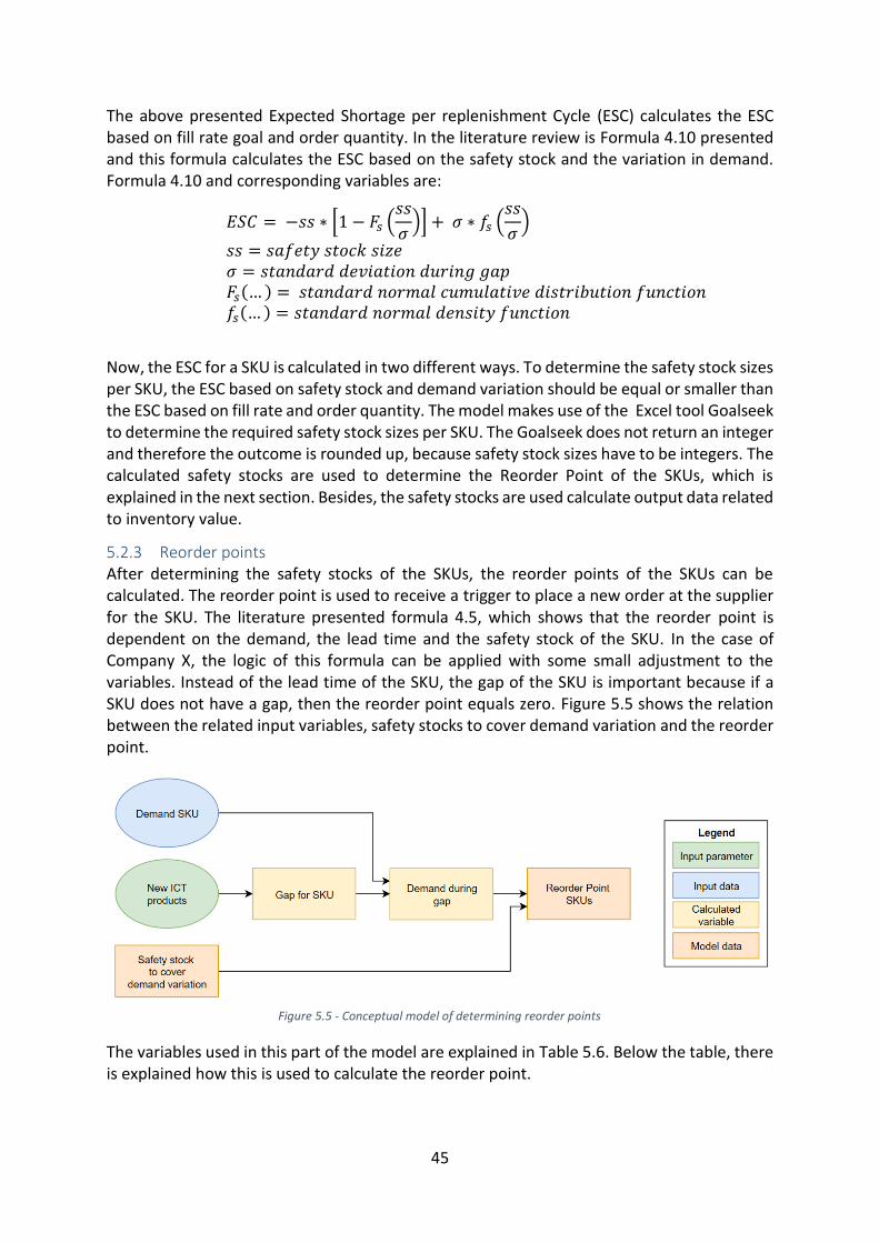
45

The above presented Expected Shortage per replenishment Cycle (ESC) calculates the ESC based on fill rate goal and order quantity. In the literature review is Formula 4.10 presented and this formula calculates the ESC based on the safety stock and the variation in demand. Formula 4.10 and corresponding variables are:

𝐸𝑆𝐶 = −𝑠𝑠 ∗ [1 − 𝐹𝑠 (𝑠𝑠

𝜎)] + 𝜎 ∗ 𝑓𝑠 (

𝑠𝑠

𝜎)

𝑠𝑠 = 𝑠𝑎𝑓𝑒𝑡𝑦 𝑠𝑡𝑜𝑐𝑘 𝑠𝑖𝑧𝑒 𝜎 = 𝑠𝑡𝑎𝑛𝑑𝑎𝑟𝑑 𝑑𝑒𝑣𝑖𝑎𝑡𝑖𝑜𝑛 𝑑𝑢𝑟𝑖𝑛𝑔 𝑔𝑎𝑝 𝐹𝑠(… ) = 𝑠𝑡𝑎𝑛𝑑𝑎𝑟𝑑 𝑛𝑜𝑟𝑚𝑎𝑙 𝑐𝑢𝑚𝑢𝑙𝑎𝑡𝑖𝑣𝑒 𝑑𝑖𝑠𝑡𝑟𝑖𝑏𝑢𝑡𝑖𝑜𝑛 𝑓𝑢𝑛𝑐𝑡𝑖𝑜𝑛 𝑓𝑠(… ) = 𝑠𝑡𝑎𝑛𝑑𝑎𝑟𝑑 𝑛𝑜𝑟𝑚𝑎𝑙 𝑑𝑒𝑛𝑠𝑖𝑡𝑦 𝑓𝑢𝑛𝑐𝑡𝑖𝑜𝑛

Now, the ESC for a SKU is calculated in two different ways. To determine the safety stock sizes per SKU, the ESC based on safety stock and demand variation should be equal or smaller than the ESC based on fill rate and order quantity. The model makes use of the Excel tool Goalseek to determine the required safety stock sizes per SKU. The Goalseek does not return an integer and therefore the outcome is rounded up, because safety stock sizes have to be integers. The calculated safety stocks are used to determine the Reorder Point of the SKUs, which is explained in the next section. Besides, the safety stocks are used calculate output data related to inventory value.

5.2.3 Reorder points After determining the safety stocks of the SKUs, the reorder points of the SKUs can be calculated. The reorder point is used to receive a trigger to place a new order at the supplier for the SKU. The literature presented formula 4.5, which shows that the reorder point is dependent on the demand, the lead time and the safety stock of the SKU. In the case of Company X, the logic of this formula can be applied with some small adjustment to the variables. Instead of the lead time of the SKU, the gap of the SKU is important because if a SKU does not have a gap, then the reorder point equals zero. Figure 5.5 shows the relation between the related input variables, safety stocks to cover demand variation and the reorder point.

The variables used in this part of the model are explained in Table 5.6. Below the table, there is explained how this is used to calculate the reorder point.

Figure 5.5 - Conceptual model of determining reorder points

46

Table 5.6 - Variables related to the reorder point of a SKU

Variable Description

Demand SKUs The following formula from Table 5.4 is again applied:

𝐷𝑒𝑚𝑎𝑛𝑑 𝑆𝐾𝑈 = 𝑚𝑎𝑥 (90 𝑑𝑎𝑦𝑠 𝑑𝑒𝑚𝑎𝑛𝑑

90,

180 𝑑𝑎𝑦𝑠 𝑑𝑒𝑚𝑎𝑛𝑑

180) ( 5.2 )

New ICT product

The obtained new ICT of the products in the model.

Gap for SKU The definition and formula is the same as in Table 5.4: 𝐺𝑎𝑝 𝑓𝑜𝑟 𝑆𝐾𝑈 = 𝑚𝑎𝑥 (𝐿𝑇 𝑆𝐾𝑈 + 𝑀𝐶𝑇 𝑝𝑟𝑜𝑑𝑢𝑐𝑡 − 𝐼𝐶𝑇 𝑝𝑟𝑜𝑑𝑢𝑐𝑡, 0) ( 5.5 )

Demand during gap

The definition and formula is the same as in Table 5.4: 𝐷𝑒𝑚𝑎𝑛𝑑 𝑑𝑢𝑟𝑖𝑛𝑔 𝑔𝑎𝑝 = 𝐷𝑎𝑖𝑙𝑦 𝑑𝑒𝑚𝑎𝑛𝑑 𝑆𝐾𝑈 ∗ 𝐺𝑎𝑝 𝑓𝑜𝑟 𝑆𝐾𝑈 ( 5.6 )

The input variables are used to calculate the reorder point. This is done by with the following formula, which is a modification of formula 4.5:

𝑅𝑒𝑜𝑟𝑑𝑒𝑟 𝑝𝑜𝑖𝑛𝑡 = 𝐺𝑎𝑝 𝑓𝑜𝑟 𝑆𝐾𝑈 ∗ 𝐷𝑒𝑚𝑎𝑛𝑑 𝑝𝑒𝑟 𝑑𝑎𝑦 + 𝑆𝑎𝑓𝑒𝑡𝑦 𝑠𝑡𝑜𝑐𝑘 𝑡𝑜 𝑐𝑜𝑣𝑒𝑟 𝑑𝑒𝑚𝑎𝑛𝑑 𝑣𝑎𝑟𝑖𝑎𝑡𝑖𝑜𝑛

The reorder points will be used in the inventory policies of the SKUs. The parts of the model described in this Section 5.2 determines for every SKU is the order quantity, safety stocks and reorder point determined. In the coming sections, this is used to determine the output data and measure the resulting inventory value, annual costs, performance and financial risks.

5.3 Output After determining the parameters of the inventory policies for every SKU, the resulting performances have to be calculated. As presented in the overview of the model, the inventory value, annual costs, financial risks and performances have to be measured. Therefore, the model calculates the output data based on both the input data and calculated model data. The outcome of the model consist of the following measurements:

- Inventory value - Cycle inventory - Safety stock - Inventory turnover

- Annual costs - Ordering costs - Holding costs

- Financial risks - Open PO value - Liability before SO - Stock of LLI needed

- Performances - ICT reduction - OLT reduction

47

5.3.1 Inventory value As presented in the conceptual model, part of the performances are the inventory value resulting from the inventory policy. Therefore, the model has to quantify this with monetary value and the inventory turnover, which is a KPI of Company X. The inventory value is dependent on the order quantities, safety stocks and standard costs of the SKUs. The order quantities of the SKUs determine the average cycle inventory of the SKU. Next to this, in the previous sections the calculation of the safety stocks is explained and this outcome is used to determine the value of safety stock. Thereafter, the total inventory value resulting from both cycle inventory and safety stock is calculated. This outcome is used together with the expected cost of goods sold to determine the inventory turnover. The relationships between all those variables are displayed in Figure 5.6.

As shown in the figure above, there is different data related to the performances with respect to inventory value. The variables and calculations are shortly described in Table 5.7.

Table 5.7 - Variables related to the inventory value performances

Variable Description

Demand SKUs The annual demand is again used in this part of the model to calculate the cost of goods sold per year. Therefore, the same formula as mentioned in Table 5.1 is applied:

𝐷𝑒𝑚𝑎𝑛𝑑 𝑆𝐾𝑈 = 𝑚𝑎𝑥 (90 𝑑𝑎𝑦𝑠 𝑑𝑒𝑚𝑎𝑛𝑑

90∗ 365,

180 𝑑𝑎𝑦𝑠 𝑑𝑒𝑚𝑎𝑛𝑑

180∗ 365) ( 5.7 )

Standard cost SKUs

The standard cost of one SKU committed with the supplier.

Costs of goods sold per year

The costs of goods sold per year are dependent on the annual demand of SKUs and the standard cost of SKUs. The cost of goods sold per year can be calculated per SKU and thereafter the sum of this for all SKUs involved is the total costs of goods sold per year, which results in the following formula:

Figure 5.6 - Conceptual model of determining inventory value performances

48

𝐶𝑜𝑠𝑡 𝑜𝑓 𝑔𝑜𝑜𝑑𝑠 𝑠𝑜𝑙𝑑 𝑝𝑒𝑟 𝑦𝑒𝑎𝑟 = ∑ 𝐷𝑒𝑚𝑎𝑛𝑑 𝑆𝐾𝑈 ∗ 𝑆𝑡𝑎𝑛𝑑𝑎𝑟𝑑 𝑐𝑜𝑠𝑡 𝑆𝐾𝑈 ( 5.8 )

Order quantities SKUs

The outcome of the model described in Section 5.2.1

Average cycle inventory

The average cycle inventory is dependent on the order quantities and the standard cost of the SKU. The assumption is made that demand is pretty constant and therefore the average cycle inventory is half of the order quantity for every SKU.

𝐴𝑣𝑒𝑟𝑎𝑔𝑒 𝑐𝑦𝑐𝑙𝑒 𝑖𝑛𝑣𝑒𝑛𝑡𝑜𝑟𝑦(€) = ∑(𝑂𝑟𝑑𝑒𝑟 𝑞𝑢𝑎𝑛𝑡𝑖𝑡𝑦

2∗ 𝑆𝑡𝑎𝑛𝑑𝑎𝑟𝑑 𝑐𝑜𝑠𝑡) ( 5.9 )

Safety stocks to cover average demand

The outcome of the model described in Section 5.2.2.

Safety stock to cover demand variation

The outcome of the model described in Section 5.2.2.

Safety stock The total safety stock needed to achieve the required ICT is the sum of the safety stock to cover average demand and the safety stock to cover demand variation.

Total average inventory

The total average inventory is the sum of the cycle inventory and the safety stock. Therefore, the following formula is used: 𝑇𝑜𝑡𝑎𝑙 𝑎𝑣𝑒𝑟𝑎𝑔𝑒 𝑖𝑛𝑣𝑒𝑛𝑡𝑜𝑟𝑦 = 𝐴𝑣𝑒𝑟𝑎𝑔𝑒 𝑐𝑦𝑐𝑙𝑒 𝑖𝑛𝑣𝑒𝑛𝑡𝑜𝑟𝑦 + 𝑆𝑎𝑓𝑒𝑡𝑦 𝑠𝑡𝑜𝑐𝑘 ( 5.10 )

Inventory turnover

The inventory turnover measures how effectively inventory is managed by comparing cost of goods sold with average inventory for a period. This measures how many times average inventory is sold during a period. The following formula is applied to calculate this:

𝐼𝑛𝑣𝑒𝑛𝑡𝑜𝑟𝑦 𝑡𝑢𝑟𝑛𝑜𝑣𝑒𝑟 =𝐶𝑜𝑠𝑡 𝑜𝑓 𝑔𝑜𝑜𝑑𝑠 𝑠𝑜𝑙𝑑 𝑝𝑒𝑟 𝑦𝑒𝑎𝑟

𝐴𝑣𝑒𝑟𝑎𝑔𝑒 𝑖𝑛𝑣𝑒𝑛𝑡𝑜𝑟𝑦 € ( 5.11 )

49

5.3.2 Annual costs Another measurement of performances are the annual costs resulting from the applied inventory management. These annual costs can be divided into annual ordering costs and annual holding costs. The annual ordering costs depends on the cost of placing an order and the number of orders per year. The number of order per year is dependent on the order quantity and annual demand of the SKUs. Next to this, the annual holding costs is dependent on the total average inventory and the holding cost rate. Figure 5.7 displays the relationships between the variables related to the annual costs.

As shown in the figure above, there is different data required to calculate the annual costs of the selected inventory management. This data varies from input data, model data and performances calculated in other parts of the model. The variables and calculations are shortly described in Table 5.8.

Table 5.8 - Variables related to annual costs performances

Variable Description

Order costs The cost of placing and processing one purchase order by Company X. The order costs at Company X are € 29,40 per order and in Section 5.2.1 is the explanation behind this variable presented.

Order quantities SKUs

The outcome of the model described in Section 5.2.1.

Demand SKUs The annual demand is again used in this part of the model to calculate the cost of goods sold per year. Therefore, the same formula as mentioned in Table 5.1 is applied:

𝐷𝑒𝑚𝑎𝑛𝑑 𝑆𝐾𝑈 = 𝑚𝑎𝑥 (90 𝑑𝑎𝑦𝑠 𝑑𝑒𝑚𝑎𝑛𝑑

90∗ 365,

180 𝑑𝑎𝑦𝑠 𝑑𝑒𝑚𝑎𝑛𝑑

180∗ 365)( 5.12 )

Figure 5.7 - Conceptual model of determining annual costs performances

50

Annual orders SKUs

The annual orders per SKU are dependent on the selected order quantity and the demand of the SKU. Therefore the following formula is applied:

𝐴𝑛𝑛𝑢𝑎𝑙 𝑜𝑟𝑑𝑒𝑟𝑠 𝑎𝑙𝑙 𝑆𝐾𝑈𝑠 = ∑𝐷𝑒𝑚𝑎𝑛𝑑 𝑆𝐾𝑈

𝑂𝑟𝑑𝑒𝑟 𝑞𝑢𝑎𝑛𝑡𝑖𝑡𝑦 𝑆𝐾𝑈 ( 5.13 )

Annual ordering costs

The annual ordering costs is the result of the annual orders multiplied with the order costs, which is equal to the following formula:

𝐴𝑛𝑛𝑢𝑎𝑙 𝑜𝑟𝑑𝑒𝑟𝑖𝑛𝑔 𝑐𝑜𝑠𝑡𝑠 = 𝐴𝑛𝑛𝑢𝑎𝑙 𝑜𝑟𝑑𝑒𝑟𝑠 𝑆𝐾𝑈𝑠 ∗ 𝑂𝑟𝑑𝑒𝑟 𝑐𝑜𝑠𝑡𝑠 ( 5.14 )

Holding cost rate The holding cost rate determines the cost of holding SKUs based on the standard cost of the SKU. The annual holding cost rate is 8.52% at Company X and in Section 5.2.1 is the calculation already shown.

Average cycle inventory

The outcome of the model described in Section 5.3.1.

Safety stocks The total safety stock needed to achieve the required ICT is the sum of the safety stock to cover average demand and the safety stock to cover demand variation.

Total average inventory

The total average inventory is the sum of the cycle inventory and the safety stock. The formula is explained in Section 5.3.1.

Annual holding costs

As mentioned earlier, the annual holding costs depends on the the value of the inventory and the holding cost rate. The value of the inventory is quantified by the total average inventory and the holding cost is determined in Section 5.2.1. This results in the following formula for the annual holding costs:

𝐴𝑛𝑛𝑢𝑎𝑙 ℎ𝑜𝑙𝑑𝑖𝑛𝑔 𝑐𝑜𝑠𝑡𝑠 = 𝑇𝑜𝑡𝑎𝑙 𝑎𝑣𝑒𝑟𝑎𝑔𝑒 𝑖𝑛𝑣𝑒𝑛𝑡𝑜𝑟𝑦 ∗ 𝐻𝑜𝑙𝑑𝑖𝑛𝑔 𝑐𝑜𝑠𝑡 𝑟𝑎𝑡𝑒( 5.15 )

5.3.3 Financial risks The last aspect of the performances related to inventory management is the financial risks. There are three different aspects of financial risks involved with inventory management in this research. First, the average value of open purchase orders to the suppliers has to be quantified. This depends on the order quantities, annual demand, lead times and standard cost of the SKUs. In the case of reducing OLTs of products, Company X has to purchase SKUs before receiving a SO from the customer. Therefore, the model has to calculate the extra liability before SO to the suppliers based on the obtained OLT. The last aspect of the financial risks is the stock of LLI needed to reduce the ICT. This depends on the safety stock to cover average demand and the safety stock to cover demand variation. All three aspects of financial risks and their related variables are shown in Figure 5.8.

51

The figure shows that there is various input necessary to calculate the financial risks involved with inventory management and the reduction of ICTs and OLTs. Therefore, Table 5.9 gives an overview of all related variables and the calculations behind some of the variables.

Table 5.9 - Variables related to the financial risks performance

Variable Description

Demand SKUs The annual demand is again used in this part of the model to determine the order interval in days. Therefore, the same formula as mentioned in Table 5.1 is applied:

𝐷𝑒𝑚𝑎𝑛𝑑 𝑆𝐾𝑈 = 𝑚𝑎𝑥 (90 𝑑𝑎𝑦𝑠 𝑑𝑒𝑚𝑎𝑛𝑑

90∗ 365,

180 𝑑𝑎𝑦𝑠 𝑑𝑒𝑚𝑎𝑛𝑑

180∗ 365) ( 5.16 )

Order quantities SKUs

The outcome of the model described in Section 5.2.1.

Order interval days

The order interval in days quantifies the average number of days between two consecutive purchase orders for a SKU. This depends on the order quantity and the annual demand of the SKU. The order interval is calculated with the following formula:

𝑂𝑟𝑑𝑒𝑟 𝑖𝑛𝑡𝑒𝑟𝑣𝑎𝑙 𝑑𝑎𝑦𝑠 = 𝑂𝑟𝑑𝑒𝑟 𝑞𝑢𝑎𝑛𝑡𝑖𝑡𝑦 𝑆𝐾𝑈

𝐴𝑛𝑛𝑢𝑎𝑙 𝑑𝑒𝑚𝑎𝑛𝑑 𝑆𝐾𝑈∗ 365 ( 5.17 )

Lead time SKUs The lead time of a SKU committed with the supplier.

Figure 5.8 - Conceptual model of determining financial risks performances

52

Average number of open orders

The average number of open orders indicates the average number of open orders based on the order interval and lead time of the SKU. If a SKU has a higher lead time then the order interval, then there is on average more than one open purchase order to the supplier. This variable is calculated with the following formula:

𝐴𝑣𝑒𝑟𝑎𝑔𝑒 𝑛𝑢𝑚𝑏𝑒𝑟 𝑜𝑓 𝑜𝑝𝑒𝑛 𝑜𝑟𝑑𝑒𝑟𝑠 =𝐿𝑒𝑎𝑑 𝑡𝑖𝑚𝑒 𝑆𝐾𝑈

𝑂𝑟𝑑𝑒𝑟 𝑖𝑛𝑡𝑒𝑟𝑣𝑎𝑙 𝑑𝑎𝑦𝑠 𝑆𝐾𝑈 ( 5.18 )

Standard cost SKUs

The standard cost of one SKU committed with the supplier.

Open PO value The open purchase order value depends on the average number of open orders, the order quantity and the standard cost per SKU. Multiplying these three variables results in the open purchase order value per SKU. Summing up this outcome for all SKUs results in the total open PO value, which results in the following formula: 𝑂𝑝𝑒𝑛 𝑃𝑂 𝑣𝑎𝑙𝑢𝑒 = ∑ 𝐴𝑣𝑔. # 𝑜𝑓 𝑜𝑝𝑒𝑛 𝑜𝑟𝑑𝑒𝑟𝑠 ∗ 𝑂𝑟𝑑𝑒𝑟 𝑞𝑢𝑎𝑛𝑡𝑖𝑡𝑦 ∗ 𝑆𝑡𝑎𝑛𝑑𝑎𝑟𝑑 𝑐𝑜𝑠𝑡 ( 5.19 )

New OLT products

The new OLT of products is variable input in the model and can be adjusted per product.

Gap for SKU The definition and formula is the same as in Table 5.4: 𝐺𝑎𝑝 𝑓𝑜𝑟 𝑆𝐾𝑈 = 𝑚𝑎𝑥 (𝐿𝑇 𝑆𝐾𝑈 + 𝑀𝐶𝑇 𝑝𝑟𝑜𝑑𝑢𝑐𝑡 − 𝐼𝐶𝑇 𝑝𝑟𝑜𝑑𝑢𝑐𝑡, 0) ( 5.20 )

Demand during gap

The definition and formula is the same as in Table 5.4: 𝐷𝑒𝑚𝑎𝑛𝑑 𝑑𝑢𝑟𝑖𝑛𝑔 𝑔𝑎𝑝 = 𝐷𝑎𝑖𝑙𝑦 𝑑𝑒𝑚𝑎𝑛𝑑 𝑆𝐾𝑈 ∗ 𝐺𝑎𝑝 𝑓𝑜𝑟 𝑆𝐾𝑈 ( 5.21 )

Minimum Order Quantity (MOQ)

This is a restriction of the supplier to purchase more than one single product per purchase order.

Exposure value for demand during gap

Obtaining shorter OLT results in purchasing SKUs before receiving a sales order. The exposure value for demand during gap calculates the involved value of purchasing SKUs before receiving a sales order. This variable depends on the demand during gap, Minimum Order Quantity and standard cost. If the MOQ of a SKU is higher than the demand during gap, then Company X has to increase their order quantity to this MOQ level. Therefore, the calculation of the exposure value for demand during gap per buy part is: 𝐸𝑥𝑝𝑜𝑠𝑢𝑟𝑒 𝑣𝑎𝑙𝑢𝑒 𝑓𝑜𝑟𝑑𝑒𝑚𝑎𝑛𝑑 𝑑𝑢𝑟𝑖𝑛𝑔 𝑔𝑎𝑝

= 𝑚𝑎𝑥(𝐷𝑒𝑚𝑎𝑛𝑑 𝑑𝑢𝑟𝑖𝑛𝑔 𝑔𝑎𝑝, 𝑀𝑂𝑄) ∗ 𝑆𝑡𝑎𝑛𝑑𝑎𝑟𝑑 𝑐𝑜𝑠𝑡 ( 5.22 )

Liability before SO

The liability before SO indicates the total value involved with purchasing before sales order. Having this liability to their suppliers is a consequence of the inventory policies applied to the SKU to shorten the OLTs. The exposure value of all SKUs have to be taken into account to calculate the liability before SO. This results in the following formula for this performance measurement:

𝐿𝑖𝑎𝑏𝑖𝑙𝑖𝑡𝑦 𝑏𝑒𝑓𝑜𝑟𝑒 𝑠𝑎𝑙𝑒𝑠 𝑜𝑟𝑑𝑒𝑟 = ∑ 𝐸𝑥𝑝𝑜𝑠𝑢𝑟𝑒 𝑣𝑎𝑙𝑢𝑒 𝑝𝑒𝑟 𝑆𝐾𝑈 ( 5.23 )

53

Safety stock to cover average demand

The outcome of the model described in Section 5.2.2.

Safety stock to cover demand variation

The outcome of the model described in Section 5.2.2.

Stock of LLI needed

The stock of LLI needed to reduce the ICTs is equal to the safety stock calculated in Section 5.3.1. The total safety stock needed to achieve the required ICT is the sum of the safety stock to cover average demand and the safety stock to cover demand variation.

5.3.4 Performances This research has to investigate if cycle times can be reduced by applying inventory management. Therefore, the reduction of ICTs of the products has to be quantified. Logically, this reduction depends on the current ICTs, the new ICTs and the demand of the products. During the modelling phase, the decision include the performances of the products related to OLT to the model, because calculations are comparable to the calculations related to the ICT. These calculations require data of the current OLTs, the new OLTs and the demand of the products. The relationships of the variables and data related to the ICT and OLT performances are shown in Figure 5.9.

The figure shows that the part of the model of ICT reduction and OLT reduction has similarities. The related variables and calculations are explained in Table 5.10.

Figure 5.9 - Conceptual model of determining ICT and OLT performances

54

Table 5.10 - Variables related to the ICT and OLT performance

Variable Description

Current ICT products

The first step in this part of the model is determining the current ICT of the products. The ICT is dependent on the lead time of SKUs and the remaining MCT for the SKUs. The lead time of SKUs and remaining MCT for the SKUs are determined based on the data in the ERP-system. The SKU with the highest sum of the lead time of the supplier and the remaining MCT determines the ICT of the product. This results in the following formula to calculate the ICT, where the maximum value over all SKUs is taken:

𝐼𝐶𝑇 𝑝𝑟𝑜𝑑𝑢𝑐𝑡 =𝑚𝑎𝑥

𝑜𝑣𝑒𝑟 𝑆𝐾𝑈𝑠(𝐿𝑒𝑎𝑑 𝑡𝑖𝑚𝑒 𝑆𝐾𝑈 + 𝑟𝑒𝑚𝑎𝑖𝑛𝑖𝑛𝑔 𝑀𝐶𝑇 𝑓𝑜𝑟 𝑆𝐾𝑈) ( 5.24 )

New ICT products

The new ICT of products is variable input in the model and can be adjusted per product.

ICT reduction per product

The ICT reduction per product indicates the improvement with respect to the current ICT. The delta between the current and new ICT can be divided by the current ICT to determine the ICT reduction per product, which is also displayed in this formula:

𝐼𝐶𝑇 𝑟𝑒𝑑𝑢𝑐𝑡𝑖𝑜𝑛 𝑝𝑒𝑟 𝑝𝑟𝑜𝑑𝑢𝑐𝑡 (%) = 𝐶𝑢𝑟𝑟𝑒𝑛𝑡 𝐼𝐶𝑇−𝑁𝑒𝑤 𝐼𝐶𝑇

𝐶𝑢𝑟𝑟𝑒𝑛𝑡 𝐼𝐶𝑇 ( 5.25 )

Demand products

The annual demand of products is calculated with the same formulae as the annual demand for SKUs. Therefore, the same formula as mentioned in Table 5.1 is applied:

𝐷𝑒𝑚𝑎𝑛𝑑 𝑝𝑟𝑜𝑑𝑢𝑐𝑡𝑠 = 𝑚𝑎𝑥 (90 𝑑𝑎𝑦𝑠 𝑑𝑒𝑚𝑎𝑛𝑑

90∗ 365,

180 𝑑𝑎𝑦𝑠 𝑑𝑒𝑚𝑎𝑛𝑑

180∗ 365) ( 5.26 )

ICT reduction The total performances related to the ICT reduction can be calculated with the current ICT, ICT reduction and the annual demand. The annual demand is added because an ICT reduction of a product with a higher demand rate contributes more to the ICT reduction than a product with a lower demand rate. The following formula is used to determine the value of this performance measurement:

𝐼𝐶𝑇 𝑟𝑒𝑑𝑢𝑐𝑡𝑖𝑜𝑛 (%) = ∑(𝐶𝑢𝑟𝑟𝑒𝑛𝑡 𝐼𝐶𝑇∗𝐼𝐶𝑇 𝑟𝑒𝑑𝑢𝑐𝑡𝑖𝑜𝑛∗𝐴𝑛𝑛𝑢𝑎𝑙 𝑑𝑒𝑚𝑎𝑛𝑑)

∑(𝐶𝑢𝑟𝑟𝑒𝑛𝑡 𝐼𝐶𝑇∗𝐴𝑛𝑛𝑢𝑎𝑙 𝑑𝑒𝑚𝑎𝑛𝑑) ( 5.27 )

Current OLT products

This is the committed OLT between Company X and the customer for a specific product. The OLT per product is retrieved from the current data of Company X and varies within a range of 5 weeks until 35 weeks.

New OLT products

The new OLT of products is variable input in the model and can be adjusted per product.

OLT reduction per product

The OLT reduction per product indicates the improvement with respect to the current OLT. The delta between the current and new OLT can be divided by the current OLT to determine the OLT reduction per product, which is also displayed in this formula:

𝑂𝐿𝑇 𝑟𝑒𝑑𝑢𝑐𝑡𝑖𝑜𝑛 𝑝𝑒𝑟 𝑝𝑟𝑜𝑑𝑢𝑐𝑡 (%) = 𝐶𝑢𝑟𝑟𝑒𝑛𝑡 𝑂𝐿𝑇 − 𝑁𝑒𝑤 𝑂𝐿𝑇

𝐶𝑢𝑟𝑟𝑒𝑛𝑡 𝑂𝐿𝑇 ( 5.28 )

55

OLT reduction The total performances related to the OLT reduction can be calculated with the current OLT, OLT reduction and the annual demand. The annual demand is added because an ICT reduction of a product with a higher demand rate contributes more to the OLT reduction than a product with a lower demand rate. The following formula is used to determine the value of this performance measurement:

𝑂𝐿𝑇 𝑟𝑒𝑑𝑢𝑐𝑡𝑖𝑜𝑛 (%) = ∑(𝐶𝑢𝑟𝑟𝑒𝑛𝑡 𝑂𝐿𝑇∗𝑂𝐿𝑇 𝑟𝑒𝑑𝑢𝑐𝑡𝑖𝑜𝑛∗𝐴𝑛𝑛𝑢𝑎𝑙 𝑑𝑒𝑚𝑎𝑛𝑑)

∑(𝐶𝑢𝑟𝑟𝑒𝑛𝑡 𝑂𝐿𝑇∗𝐴𝑛𝑛𝑢𝑎𝑙 𝑑𝑒𝑚𝑎𝑛𝑑) ( 5.29 )

5.3.5 Dashboard The previous sections elaborated on the performances measurement of the model and related calculations. The model execute these calculations in several Worksheets in Excel. For this reason, there is developed a dashboard to present the key outcomes to the user. The dashboard has several buttons to import actual data from the ERP-system or execute calculations based on the input parameters. These buttons are placed in the middle of the dashboard. The input parameters are presented in the left part of the dashboard. The user can adjust these parameters easily before executing calculations. Next to this, the outcome related to inventory value, annual costs, ICT and OLT performance and financial risks are presented in the right part of the model. The dashboard is used in the analysis phase to compare outcomes and give insights in the performances related to inventory management. Figure 5.10 gives a visual impression of the dashboard. Unfortunately, other parts of the model can not be shown in detail due to confidentiality of the information.

Figure 5.10 - Dashboard of the model

56

5.4 Conclusion This chapter elaborated on the created model related to cycle time reduction by inventory management. By explaining the created model, this chapter answers the third research question:

What are the performances of the alternatives regarding the cycle times and the other KPIs of Company X in a model/simulation?

The model has to give insights in several performances resulting from cycle time reduction by inventory management. As described in Section 5.3, the following performances have to be quantified by the model:

- Inventory value - Cycle inventory - Safety stock - Inventory turnover

- Annual costs - Ordering costs - Holding costs

- Performance - ICT reduction - OLT reduction

- Financial risk - Open PO value - Liability before SO - Stock of LLI needed

This outcome depends on the scope of the model, because the number of products as input is variable. In the next chapter, the decision is made to focus on a selection of products for further analysis. Next to this, the model is data driven and therefore the assumption is made that the data in the ERP-system is correct. In the conceptual model is defined, that the following input data has to be available or determined during this research:

- SKU demand - Product demand - SKU characteristics - Product characteristics - Order costs at Company X - Holding cost rate at Company X

The final output of the model is a dashboard, which presents the values of the above described performances. These performances are dependent on the selected parameters and applied inventory management. The applied inventory management means an inventory policy for every SKU involved with the products in the scope of the model. These inventory policies consists of order quantities, safety stocks and reorder points.

57

6 Model analysis The previous chapter described the constructed model during this research. The model calculates the output and performances needed to investigate the relationship between cycle times and inventory management. First, the products in the scope of this analysis is defined in Section 6.1. The main objective of this research is ICT reduction of these products by inventory management. Therefore, Section 6.2 elaborates on the analysis of ICT reduction by applying safety stocks. Thereafter, the other performances related to inventory management and ICT are analyzed and described. Section 6.3 elaborates on the resulting inventory value, which has to give insights in cycle inventory, safety stocks and inventory turnover. Then, Section 6.4 gives insights in the annual costs related to inventory management. Next to these financial performances, Section 6.5 focusses on the performances related to ICTs and OLTs. Lastly, Section 6.6 presents an analysis of the financial risks related to inventory management and cycle time reduction. This chapter ends with Section 6.7, which gives a conclusion of the executed analysis.

6.1 Scope of the analysis In the beginning of this research, Section 2.6 elaborated on the scope of this research. In this section, the decision was made that this research should take all products of Customer Y into account. During the modelling and analysis phase, it became clear that not every product gets reliable output from the model. This was the case with NPIs or EOL products, because the demand data of these products is not steady and reliable. Besides that, the customer does not request shorter ICTs for NPIs or EOL products. Therefore, the scope of this research is to 86 products. Those products are volume products of Customer Y with reliable data. The list of products involved in this analysis is given in Appendix 2. Next to this, the products are classified in four different product categories. These categories are cabinet, spare parts, small box and PCBA. Figure 6.1 shows the number of products in every category.

Figure 6.1 - Number of products per category in the scope of this analysis

58

The figure above gives insights in the number of products per category. Despite that, for Company X it is more important how much sales is generated per category. The annual sales of a product is dependent on the sales price and the annual demand per product. The model can calculate the expected annual sales of the products with data of the demand and sales prices of the products. Then, the annual sales per category is calculated by summing up the annual sales of the products in that category. Figure 6.2 presents the expected annual sales per category based on the 86 products in the scope of this analysis. The total expected annual sales is € 42,980,245 and the figure shows that cabinets have by far the highest expected annual sales. Despite that, there are just 12 products in this category. This outcome was already expected, because cabinets have higher sales prices. These insights in the products in the scope and the corresponding expected annual sales are useful to quantify the ratio of inventory value and annual costs compared to annual sales.

6.2 Safety stocks for ICT reduction The current situation analysis and literature review showed us that safety stocks should be applied to reduce the ICTs of the products of Company X. In Section 5.2.2 is described how the safety stock sizes are related to the ICT of the products. The model distinguishes two types of safety stock and the relationship between the value of these safety stocks and the ICT is analyzed in this section.

6.2.1 Safety stock to cover average demand First, the safety stock to cover average demand to reduce the ICTs is analyzed. The calculations of this output is extensively described in Section 5.2.2. Now, the output of this part of the model is analyzed by varying the obtained ICT of the products. Varying the ICT of the products shows the amount of safety stock needed to cover the average demand of products outside this ICT. Logically, a higher ICT than the current ICT results in no safety stock. Therefore, the analysis does not need to take ICT above 40 weeks into account and the ICTs are equal for all 86 products. The input of the ICTs in the model is varied from 40 weeks until 10 weeks. Besides, the input can be adjusted per product in the model. Figure 6.3 shows the required safety stock value to cover average demand per obtained ICT.

Figure 6.2 - Expected annual sales per category

59

The figure shows that shortening the ICTs increases the value of required safety stock exponentially. This exponential increase is caused by more SKUs with safety stock and a higher safety stock value per SKU. Shortening ICTs of products results in more SKUs with a gap with this ICT, which results in more SKUs with a required safety stock to achieve this ICT. Next to this, shortening ICTs results for SKUs in higher gaps with the ICT, which results in more demand to cover with safety stocks. These two factors together result in the exponential growth of safety stock to cover average demand while shortening ICTs. During this analysis, the decision is made to focus on a scenario of an ICT of 16 weeks and get insights in the outcome resulting from this ICT. In the case of an ICT of 16 weeks, the value of the safety stock to cover average demand is € 862,765.

Logically, not every SKU needs safety stocks and therefore is the safety stock value not equal for every SKU. Therefore, it can be beneficial for Company X to know which SKUs require a high value of safety stock. For every SKU can be determined which percentage of safety stock value is caused by this SKU. Ranking the SKUs based on total value in descending order and calculating the cumulative percentage of the total value of the safety stocks of all SKUs results in Figure 6.4. The graph shows that a small percentage of the SKUs contribute to a big percentage of the value of safety stock to cover average demand. This shows that it can be beneficial for Company X to investigate if there are possibilities to prevent high safety stock values for these SKUs. For example, supplier involvement or lead time reduction for SKUs with a high safety stock value.

Figure 6.3 - Value of safety stock to cover average demand per ICT

60

The figure above already showed that few SKUs contribute to a large part of the safety stock value. Therefore, the ten SKUs with the highest value of safety stock to cover average demand are presented in Table 6.1. Besides, the model provides a complete overview of the value of stock for all SKUs, which can be easily sorted from high to low values.

Table 6.1 - SKUs with highest value of safety stock to cover average demand

Part Safety stock Standard cost Value of stock

Confidential 15 € 5,316.00 € 79,740.00

Confidential 120 € 627.27 € 75,272.73

Confidential 92 € 777.03 € 71,486.48

Confidential 66 € 890.20 € 58,753.20

Confidential 9 € 5,782.52 € 52,042.68

Confidential 2238 € 16.48 € 36,882.25

Confidential 12 € 3,054.61 € 36,655.32

Confidential 24 € 1,418.00 € 34,032.00

Confidential 17 € 1,394.00 € 23,698.00

Confidential 395 € 44.70 € 17,656.50

6.2.2 Safety stock to cover demand variation Next to the safety stock to cover average demand, there is investigated how much safety stock is required to cover demand variation. The literature review presented the relationship between order quantity, the obtained fill rate and required safety stock. First, there is analyzed what the relation is between obtained fill rated, safety stocks and resulting overall fill rate. Based on Appendix 4 and the expertise in the company, there is decided to obtain fill

Figure 6.4 - Relation between total value of safety stock to cover average demand and number of SKUs

61

rates of 90 % for the SKUs. Then, the safety stock to cover demand variation is analyzed by varying the obtained ICT of the products. Varying the ICT of the products shows the amount of safety stock needed to cover the demand variation of products outside this ICT. A higher ICT than the current ICT results in no safety stock. Therefore, the analysis does not need to take ICT above 40 weeks into account and the ICTs are equal for all 86 products. The model is run for ICTs from 40 weeks until 10 weeks. Figure 6.5 shows the required safety stock value to cover demand variation per obtained ICT with an obtained fill rate of 90%.

This figure also shows that shortening the ICTs increases the value of required safety stock exponentially. This exponential increase is caused by more SKUs with safety stock and a higher safety stock value per SKU. Shortening ICTs of products results in more SKUs with a gap with this ICT, which results in more SKUs with demand variation to cover. Next to this, shortening ICTs results for SKUs in higher gaps with the ICT, which results in more demand variation to cover with safety stocks. These two factors together result in the exponential growth of safety stock to cover demand variation while shortening ICTs. During this analysis, the decision is made to focus on a scenario of an ICT of 16 weeks and get insights in the outcome resulting from this ICT. In the case of an ICT of 16 weeks, the value of the safety stock to cover demand variation is € 133,148.

There is again investigated how the cumulative percentage of the total value of the safety stocks is related to the cumulative percentage of all SKUs. Figure 6.6 shows that an extremely small percentage of the SKUs contribute to a big percentage of the value of safety stock to cover demand variation. This shows that it can be beneficial for Company X to investigate if there are possibilities to prevent high safety stock values for these SKUs. For example, supplier involvement or lead time reduction for SKUs with a high safety stock value.

Figure 6.5 - Value of safety stock to cover demand variation per ICT

62

The figure above shows that a couple of SKU are the main contributors of the safety stock to cover demand variation. Therefore, the ten SKUs with the highest value of safety stock to cover demand variation are presented in Table 6.2. And again, the model provides a complete overview of the value of safety stock for all SKUs, which can be easily sorted from high to low values.

Table 6.2 - SKUs with highest value of safety stock to cover demand variation

Part Safety stock Standard cost Value safety stock

Confidential 3 € 5,316.00 € 15,948.00

Confidential 13 € 890.20 € 11,572.60

Confidential 2 € 5,782.52 € 11,565.04

Confidential 7 € 1,418.00 € 9,926.00

Confidential 3 € 3,054.61 € 9,163.83

Confidential 11 € 777.03 € 8,547.30

Confidential 13 € 627.27 € 8,154.55

Confidential 5 € 1,394.00 € 6,970.00

Confidential 2 € 2,287.00 € 4,574.00

Confidential 248 € 16.48 € 4,087.04

6.2.3 Total safety stocks value In the sections above, the two types of safety stocks are analyzed. This analysis showed that shortening ICTs results in an exponential growth of both types of safety stocks. Besides, the analysis gave the insights that the safety stocks to cover average demand are significantly higher than the safety stocks to cover demand variation. As mentioned earlier, both types of safety stock are required to achieve the ICT reduction. Therefore, the sum of both safety stocks calculated per obtained ICT. Figure 6.7 displays the total value of safety stock required per obtained ICT. Logically, this figure shows again an exponential increase of the safety stock while reducing the ICT. The scenario of an ICT of 16 weeks results in a total safety stock value of € 995,913. The value of this safety stock is equal to 2.3% of the expected annual sales of the products in the scope of this research. Table 6.1 and Table 6.2 already showed that a small

Figure 6.6 - Relation between total value of safety stock to cover demand variation and number of SKUs

63

number of SKUs have a high value of safety stock. For the total safety stock required for an ICT of 16 weeks, 10 SKUs cause more than half of the value of the safety stock.

6.3 Inventory value Another important performance measurement of inventory management is the inventory value. Therefore, the model has to give insights in the cycle inventory, safety stock and resulting inventory turnover. These performances are dependent on the order quantities and safety stocks of SKUs. First, there is analyzed how cycle inventory is related to order quantities. Thereafter, the safety stocks of previous section are shortly discussed before the total inventory value and resulting inventory turnover are presented.

6.3.1 Cycle inventory The decision is made during this research to determine order quantities in the model based on the EOQs. Section 5.2.1 presented how the EOQ is applied in the constructed model and Section 5.3.1 shows how the model determines the resulting average cycle inventory. During the analysis of cycle inventory, there is added a restriction that the order quantity should not be higher than the demand for a variable number of months. This number of months is varied from one month of demand to twelve months of demand. By adding this restriction, Company X can prevent ordering to much of an SKU that could result in excess and obsolete inventory. With the use of the model, the average cycle inventory given this restriction is calculated and the outcome is presented in Figure 6.8. The figure shows that restricting the order quantities with a maximum of one month of demand results in the lowest average cycle inventory. Despite, this would result in ordering SKUs twelve times a year and this increases annual ordering costs. Next to this, relaxation of the restriction results in a higher average cycle inventory. Despite that, the figure shows that as the restriction further eases, the average cycle inventory increases less. Given this figure, the influence of this restriction on annual costs and the corporate goal to obtain an inventory turnover of 6.5, there is decided to restrict the order quantities with a maximum of three months of demand. This results in an average cycle inventory of € 2,066,545. The influence of this decision on the annual costs are presented in Section 6.4.

Figure 6.7 - Total value of safety stock per ICT

64

6.3.2 Safety stock The second aspect of inventory turnover is safety stock. In Section 6.2 is described which safety stocks are required to reduce the ICT to 16 weeks. Next to this, Company X has already safety stock for some of the SKUs in the scope of this analysis. The current value of this safety stock at Company X is € 320,645. Customer Y requested and pay for a large part of this safety stock, because of historical events in the supplier market for those SKUs. This invoiced safety stock has a value of € 251,075. Therefore, this safety stock cannot be reduced and has to be added to the calculated safety stock in Section 6.2. Despite, the remaining safety stock of € 69,570 can be replaced by the safety stock calculated in Section 6.2. In the next section, the total inventory value and resulting inventory turnover is further analyzed.

6.3.3 Inventory turnover The previous two sections gave insights in the cycle inventory and safety stocks resulting from applying inventory management. After analyzing these two outcomes separately, they are added to each other to calculate the total average inventory value. Section 5.3.1 described how this average inventory value is calculated and used to determine the inventory turnover. The outcome of the model has to be compared with the current inventory value at Company X. This inventory value consists of the cycle inventory, invoiced safety stock and extra safety stock. The current inventory value is calculated based on the data in the ERP-system. Figure 6.9 shows a comparison of the average inventory value based on the current situation and the model. The figure shows that the current situation has € 1,865,699 more cycle inventory compared to the model. This shows that Company X does not manage their inventory optimally. In the current situation is around one million of inventory caused by just 19 SKUs. By applying the EOQs to SKUs, the inventory levels of expensive SKUs are much lower which reduces the cycle inventory value. Besides, the extra safety stocks in the model are higher because of the obtained ICT reduction. Combining these aspects together, the total average

Figure 6.8 - Relationship between cycle inventory and restricted order quantities

65

inventory value reduces with € 939,356 for the involved SKUs. This is a 22.1% reduction of the current inventory value.

After determining the inventory value, the inventory turnover can be calculated and analyzed. Section 5.3.1 elaborated on the relationship between inventory value, costs of goods per year and resulting inventory turnover. The inventory value is known in the current situation and the inventory value is calculated based on the model. The cost of goods per year is equal for both and depends on the annual demand and standard cost of SKUs. The model calculated the cost of goods per year on € 28,441,740. This results in an inventory turnover for the SKUs of 6.7 in the current situation. Despite that, the inventory value of the proposed model results in an inventory turnover of 8.6. This is a significant increase of the inventory turnover of 28.3%. Besides, this is far above the corporate goal for inventory turnover of 6.5. This means that the inventory policies of the model makes sure that SKUs spend in general a shorter time in the warehouse before it is assembled at Company X.

6.4 Annual costs The second type of performance measurements are related to the annual costs of inventory management and calculations are described in Section 5.3.2. These annual costs consists of ordering costs and holdings costs. As mentioned earlier, EOQs are applied to optimize the annual costs related to inventory management by making the tradeoff between order costs and holding costs. In the previous section, the restriction related to order quantities is explained related to cycle inventory. In the analysis of annual costs is again this restriction

Figure 6.9 - Comparison of average inventory value

66

applied to order quantities, but now the relationship between annual order costs and holdings costs is analyzed. Thereafter, the current situation with respect to annual costs is compared to the annual costs based on the model.

6.4.1 Ordering costs The annual ordering costs depends on the number of orders per year. By calculating the annual orders per year, the annual ordering costs are sequentially calculated. The relationship between annual order costs and the restriction with respect to order quantities is analyzed. Figure 6.10 shows that easing the restriction results in lower annual order costs. Logically, restricting order quantities to a maximum of one month of demand results in more orders per year, which causes higher annual order costs. Despite, the EOQ makes a tradeoff between order costs and holding costs and therefore the influence of the restriction on holding costs need to be analyzed as well.

Figure 6.10 - Relationship between annual order costs and restricted order quantities

67

6.4.2 Holding costs The annual holding costs is dependent on the average inventory value, which depends on the average cycle inventory, invoiced safety stock and extra safety stock. Section 6.3 elaborated on the inventory value and this is used in the calculation of holding costs. In this section, the cycle inventory is again determined given the restriction related to order quantities. Besides, the safety stocks are equal to the safety stocks presented in Figure 6.9. Figure 6.11 shows the relationship between annual holding costs and the restriction with respect to order quantities. Easing the restriction results in higher annual order costs, because cycle inventories increase as already discussed in Section 6.3.1. In the next section, ordering costs and holding costs needs to be summed up because the EOQ should minimize the total annual costs of both together.

6.4.3 Total annual costs In the previous two section is the relationship between ordering and holding costs with the restriction on order quantities analyzed. By summing up both types of costs, the annual costs of inventory management is calculated. Figure 6.12 displays how the total annual costs decreases when the restriction on order quantities relaxes. After analyzing both Figure 6.12 and Figure 6.8, the decision is made to have a maximum order quantity of three months of demand per SKU. The reason for this is that the annual costs decrease slowly after relaxing the restriction more, but the financial risks increases when ordering more months of demand. And as mentioned before, restricting the order quantities on a maximum of three months of demand is in line with the corporate goal for inventory turnover.

Figure 6.11 - Relationship between annual holding costs and restricted order quantities

68

After selecting a maximum months of demand for the order quantities, the annual costs of the current situation can be compared with the model. Therefore, the annual holding costs in the current situation are based on the inventory value as mentioned in Section 6.3.3. The ordering costs in the current situation are based on the number of orders in the past twelve months for the involved SKUs. There were placed 19,731 orders in the past twelve months instead of 11,308 order resulting from the inventory management suggested by the model. The resulting ordering costs and holding cost are displayed in Figure 6.13. The inventory management suggested by the model results in a cost reduction of € 327,669 per year. This reduces the annual costs of inventory management of the involved SKUs with 34.8 %.

Figure 6.12 - Relationship between total annual costs and restricted order quantities

69

6.5 Financial risks The third type of performance measurements are related to the financial risks related to the applied inventory management. In Section 5.3.4 is described how these measurements are calculated in the model. These measurements will be quantified in this section to indicate the risks resulting from inventory management, OLT reduction and ICT reduction.

6.5.1 Open PO value Next to the cycle inventory and safety stock is the amount of open purchase orders to the suppliers important financial aspect of inventory management. Section 5.3.3 elaborates on the calculations of the open PO value and relates variables. The open PO value depends on the order quantities determined by the model. In this analysis again the order quantities are restricted to a quantity lower or equal to three months of demand. The current open PO value is determined based on the data in the ERP-system and compared with the outcome of the model. Figure 6.14 shows the comparison of open PO value of the current situation and the model. Applying the order quantities of the model results in a reduction of open PO value of € 686,378. This is a reduction of 13.1% of the open PO value based on the current situation.

Figure 6.13 - Comparison between annual costs of inventory management

70

6.5.2 Liability before SO During the model phase is decided to include OLT reduction in the model next to ICT reduction. OLT reduction can be applied by purchasing components before the sales order of the customer is received. Therefore, the model has to calculate the liability before SO and in Section 5.3.3 is this explained. This calculation has overlap with the calculation of safety stock needed to cover average demand. Therefore, there is analyzed how the liability before sales order is dependent on the obtained OLT for the products. In the analysis, the obtained OLTs are varied from 40 weeks to 5 weeks. Figure 6.15 shows how the liability before SO exponentially increases if he obtained OLT decreases. This is caused by the fact that more SKUs need to be ordered before SO and next to this, the needed quantity to be ordered per SKU increases as well. This insights with respect to OLT of products can be applied in the future if the customer requests for shorter OLTs.

6.5.3 Stock of LLI needed The last financial risk related to inventory management is stock of long lead time items. This part of the model is again described in Section 5.3.3. In that section is explained that the stock of LLIs is the sum of both types of safety stocks. The relationship between the total value of safety stock and obtained ICT is analyzed in Section 6.2.3. The outcome of this analysis is therefore exactly the same for the stock of LLI needed.

Figure 6.14 - Comparison of open PO value

71

6.6 Performances The last performance measurements are related to the improvement of the ICTs and OLTs. In Section 5.3.4 is described how this part this performance measurement is included in the model. The ICT reduction is possible by applying safety stocks for SKUs, which is presented in Section 6.2. Besides that, the OLTs can be reduced by purchasing SKUs before sales order and this results in liability before sales order, which is discussed in Section 6.5.2.

6.6.1 ICT reduction The ICT reduction is dependent on the current ICTs of the products and the corresponding demand of the products. The obtained ICT is again varied from 40 weeks to 10 weeks. Figure 6.16 shows the relationship between the percentual reduction of the ICT and the obtained ICT. Logically, obtaining a ICT of 40 weeks results in no reduction and while shortening the ICT, the percentual reduction increases exponentially. The reason for that is that shorter obtained ICTs affect more products and this increases the ICT reduction. Now, taking the scenario of an ICT of 16 weeks results in an ICT reduction of 43.1 %. As mentioned in 6.2.3, this requires a total safety stock value of € 995,913.

Figure 6.15 - Relationship between liability before SO and OLT

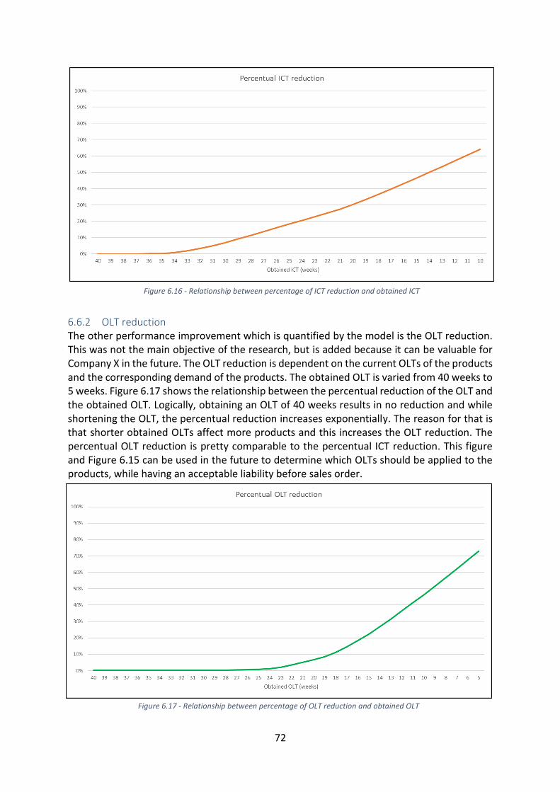
72

6.6.2 OLT reduction The other performance improvement which is quantified by the model is the OLT reduction. This was not the main objective of the research, but is added because it can be valuable for Company X in the future. The OLT reduction is dependent on the current OLTs of the products and the corresponding demand of the products. The obtained OLT is varied from 40 weeks to 5 weeks. Figure 6.17 shows the relationship between the percentual reduction of the OLT and the obtained OLT. Logically, obtaining an OLT of 40 weeks results in no reduction and while shortening the OLT, the percentual reduction increases exponentially. The reason for that is that shorter obtained OLTs affect more products and this increases the OLT reduction. The percentual OLT reduction is pretty comparable to the percentual ICT reduction. This figure and Figure 6.15 can be used in the future to determine which OLTs should be applied to the products, while having an acceptable liability before sales order.

Figure 6.16 - Relationship between percentage of ICT reduction and obtained ICT

Figure 6.17 - Relationship between percentage of OLT reduction and obtained OLT

73

6.7 Conclusion This chapter presented us an analysis of the performance measurements of the model. This gave us insights in the effects of inventory management on the inventory value, annual costs, financial risks and performances. First, the relationship between the required safety stock and the ICT of the products is extensively analyzed. This analysis showed us that the safety stocks increases exponentially if the obtained ICTs are shortened. In this analysis, there is selected a scenario of an obtained ICT of 16 weeks and fill rate goal of 90%. This scenario results in a required safety stock with a value of € 995,913. This safety stock results has annual holding costs, which are calculated with the holding cost rate and results in annual costs of € 84,852. Applying an obtained ICT of 16 weeks results in a reduction of the ICT of 43.1%.

Next to the safety stocks and ICT reduction, the inventory value is analyzed in this chapter. The application of EOQs to the SKUs can reduce the inventory value of the involved SKUs. Application of the EOQ together with applying safety stock to reduce the ICT results in a reduction of the total average inventory value of € 939,356. This is a 22.1% reduction of the current inventory value. Reducing the inventory value results in an improvement of the inventory turnover from 6.7 to 8.6.

Another aspect of inventory management is the resulting annual costs, which is also analyzed. The application of EOQs to the SKU contribute in a positive way to the inventory value, but the number of orders for the SKU do also decrease compared to the current situation. This results in annual savings of € 349,061 compared to the current annual costs. This reduces the annual costs of ordering and holding SKUs with 37.0%.

Lastly, the financial risks resulting from applying a certain way of inventory management. The application of EOQs results in a lower value of open PO to the suppliers. The average open PO value reduces with € 686,378 compared to the current situation, which is a reduction of 13.1%. Next to this, the financial risk of OLT reduction are indicated with liability before sales order. The analysis in this chapter showed an exponential increase of the liability while shortening the obtained OLT. This knowledge and the model can be used within Company X to negotiate future OLTs of the products.

After constructing the mathematical model and executing an extensive analysis of this model, the next chapter will formulate conclusions and recommendations with respect to this research. This recommendation will focus on how the model should be used in the future to implement proper inventory management at Company X.

74

7 Conclusions and recommendations This chapter will elaborate on the conclusion and recommendations of this research. The goal of this research was constructing a mathematical model to analyze Integral Cycle Times (ICT) reduction by inventory management. Therefore, the following research question had to be answered:

Which inventory policy should be used at Company X to reduce the Integral Cycle Times of the products for Customer Y taking into account financial risks and reliability risks?

First, the answer to this research question is presented together with the conclusion of this report. Thereafter, there are presented recommendations based on this research to improve the performances of Company X.

7.1 Conclusion The ICTs of the products of Company X are dependent on a couple of SKUs with a long lead time. Therefore, reducing this ICT can be achieved by applying proper inventory management. Based on the literature review, there is decided to focus on determining optimal safety stocks and order quantities for the involved SKUs. The order quantities are determined with the use of the EOQ formula while taking into account some restriction with respect to MOQs and demand of the SKU. Next to this, safety stocks have to cover demand of SKUs outside the ICT. Therefore, there are distinguished to types of safety stock, one to cover the average demand and one to cover demand variation. These safety stocks are calculated based on the average demand of the SKU and the Expected Shortage per replenishment Cycle. The analysis of the model showed us that decreasing the ICT results in an exponential increase of the total value of required safety stock. During the analysis, there is decided to point out a scenario of obtained ICTs of 16 weeks and an obtained fill rate of 90%. This scenario requires safety stock with a value of € 995,913. This amount of safety stock results in annual costs of € 84,852. On the other hand, the performances of Company X will improve and the ICTs are reduced with 43.1%. Lastly, the financial risks of this safety stock is minimized by the fact that volume products and underlying items are in the scope of this research. The chance of getting excess or obsolete inventory is small.

Another aspect of the inventory policies is the order quantity of SKUs. As mentioned above, the model determines these order quantities based on the EOQ formula. The literature review showed us that this formula optimizes the total costs of ordering and holding SKUs. The model showed us that the application of the EOQ to the SKUs involved in this research would be beneficial. This results in a total savings of the annual costs of € 327,669. These savings are 34.8 % of the current annual costs of inventory management. The main cause of lower costs is reducing the number of orders per year for the involved SKUs.

Lastly, the application of inventory management influences the inventory value of the involved SKUs. This inventory value is dependent on the cycle inventory, which effected by the application of the EOQs to the order quantities, and the safety stocks. The implementation of safety stocks for the obtained ICT of 16 weeks together with the already committed safety stock and the cycle inventory determine the total inventory value. This suggested inventory policy of the model results in a reduction of average inventory value of € 939,356, which is 22.1% reduction compared to the current situation. Next to this, the inventory turnover would increase from 6.7 to 8.6, which is far above the corporate goal of 6.5.

75

Concluding, the answer of the research question is that safety stocks should be applied for SKUs with long lead times to reduce the Integral Cycle Times of the products for Customer Y. Next to this, Company X should apply fixed order quantities for the inventory policies of the SKUs.

7.2 Recommendations The conclusion presented the answer to the research question and formulated the most important insights with respect to inventory management and ICT reduction. The model showed us that the savings of applying EOQ to the order quantities are higher than the costs of safety stocks to reduce the ICT reduction. Therefore, it is recommended to use the model as starting point to apply proper inventory management for the SKUs and reduce the ICT of the products. Important to note is that the data in the ERP-system has to be up to date and data integrity is important to make sure that the outcome of the model is valid. The calculations within the model should be updated on a regular basis, because the model execute the calculations based on the data in the ERP-system. Changes in demand data of the products are possible in the future and this influences the inventory policies of the SKUs. Next to this, Company X should consider alternatives for SKUs with a high value of inventory and/or safety stock. For example, cooperating with the supplier to reduce lead times, which reduces the amount of safety stock needed.

As already mentioned above, the application of EOQ results in savings for Company X. For this reason, it is recommended to purchase SKU with order quantities based on EOQ regardless of ICT reduction. The analysis and conclusion showed us the possible improvement of costs and inventory value compared to the current situation.

Lastly, this research and analysis of the model gave Company X insights with respect to inventory management and ICT reduction. A next step is involving the customer in the topic of ICT reduction to get a clear view on which ICTs are obtained for the involved products. Thereafter, Company X and the customer can negotiate with each other about liabilities for the inventory of LLIs. The current contracts with the customer should be reviewed. The input of the customer can be used together with the model to determine the needed inventory to improve the ICTs of the products.

Next to the recommendations mentioned above, there are some interesting topics for further research within Company X. Based on the outcomes and findings during this research it can be useful to execute a research related to the following topics: - Variability in lead times of SKU and the resulting deliver reliability of suppliers - Influence of quantity discount on the EOQs of SKUs - Improving insights in future forecast and demand of customers

76

References Axsäter, S. (2015). Inventory Control. Springer.

Company X . (2019). Retrieved from Company X

Chen, F. (1998). Echelon Reorder Points, Installation Reorder Points, and the Value of Centralized Demand Information. Management Science, 221-264.

Chopra, S., & Meindl, P. (2013). Supply Chain Management. Pearson.

Flores, B. E., & Whybark, D. C. (1986). Multiple criteria ABC analysis. International Journal of Operations & Production Management, 38-46.

Heerkens, H., & Van Winden, A. (2012). Geen Probleem. Business School Nederland.

Hopp, W., & Spearman, M. (2008). Factory Physics. Waveland Press.

Kim, C. (n.d.). prof1.incheon.ac.kr. Retrieved from Safety Inventory and Product Availability.

Kuncoro, E. G., Aurachman, R., & Santosa, B. (2018). Inventory policy for relining roll spare parts to minimize total cost of inventory with periodic review (R,s,Q) and periodic review (R,S). IOP Conference Series: Material Science and Engineering.

Radasanu, A. C. (2016). Inventory mangement, service level and safety stock. Journal of Public Administration, Finance and Law, 145-153.

Saaty, T. L. (2008). Decision making with the analytic hierarchy process. International Journal of Services Sciences, 83-98.

Silver, E. A., Pyke, D. F., & Thomas, D. J. (2017). Inventory and Production Management in Supply Chains. CRC Press.

Stoll, J., Kopf, R., Schneider, J., & Lanza, G. (2015). Criticality analysis of spare parts management: a multi-criteria classification regarding a cross-plant central warehouse strategy. In Production Engineering (pp. 225-235). Berlin Heidelberg: Springer.

Van Kampen, T. J., Akkerman, R., & van Donk, D. (2012). SKU classification: A literature review and conceptual framework. International Journal of Operations and Production Management, 850-876.

Waters, D. (2003). Inventory Control and Management. Wiley.

Yu, M.-C. (2011). Multi-criteria ABC analysis using artificial-intelligence-based classification techniques. Expert Systems with Applications - Elsevier, 3416-3421.

Zheng, Y.-S. (1992). On properties of stochastic inventory systems. Management Science, 87-103.

77

Appendices Appendix 1: Thesis planning

Activity Start week End week Duration

Problem identification 19-05 19-06 2

Research design 19-05 19-07 3

Current situation analysis 19-06 19-09 4

Literature study 19-07 19-10 4

Data gathering and analysis 19-09 19-13 5

Model construction 19-11 19-19 9

Model analysis 19-17 19-21 5

Results and implementations 19-21 19-24 4

Report and presentation 19-24 19-26 3

3

4

5

9

8

4

4

3

5 10 15 20 25

A C T I V I T Y

R E P O R T A N D P R E S E N T A T I O N

R E S U L T S A N D I M P L E M E N A T I O N S

M O D E L A N A L Y S I S

M O D E L C O N S T R U C T I O N

D A T A G A T H E R I N G A N D A N A L Y S I S

L I T E R A T U R E S T U D Y

C U R R E N T S I T U A T I O N A N A L Y S I S

R E S E A R C H D E S I G N

WEEK NUMBER

GANTT CHART THESIS PLANNING

78

Appendix 2: List of products involved in this research Removed due to confidentiality

79

Appendix 3: Demand component Y to assume normal distribution The demand per week of component Y is displayed. Based on this data is the standard deviation and average determined. Thereafter, dividing the standard deviation by the average results in a value smaller then 0.5. Therefore, the normal distribution for demand per week can be assumed. This assumption can be applied to all components.

Component Y

YearWeek Demand

201925 361

201926 587

201927 874

201928 1045

201929 546

201930 1095

201933 680

201934 737

201935 788

201936 810

201937 882

201938 480

201939 769

201940 903

201941 752

201942 624

201943 792

201944 579

201945 349

201946 459

201947 559

201948 369

201949 205

201950 162

Std. Deviation (σ) 241.675

Average (μ) 641.958

σ/μ 0.376

80

Appendix 4: Analysis of the fill rate goal