currency orders and exchange rate dynamics: an - brandeis
TRANSCRIPT

Currency Orders and Exchange Rate Dynamics: An Explanation for the Predictive Success of Technical Analysis
C. L. OSLER*
ABSTRACT This paper documents clustering in currency stop-loss and take-profit orders, and uses that clustering to provide an explanation for two familiar predictions from technical analysis: (1) trends tend to reverse course at predictable support and resistance levels, and (2) trends tend to be unusually rapid after rates cross such levels. The data are the first available on individual currency stop-loss and take-profit orders. Take-profit orders cluster particularly strongly at round numbers, which could explain the first prediction. Stop-loss orders cluster strongly just beyond round numbers, which could explain the second prediction.
May 2002 *Brandeis University, Waltham, MA 02454. [email protected] This paper has benefited extensively from thoughtful comments by an anonymous referee, as well as comments from Franklin Allen, Jose Campa, John Carlson, Rick Green, Keith Henthorn, Charles Himmelberg, Rich Lyons, Jim Mahoney, and Chris Neely. The author thanks Gijoon Hong and Priya Gandhi for excellent research assistance. Errors or omissions remain the responsibility of the author.
Exchange rate research has brought to light a robust but unexplained result: Technical analysis is
useful for predicting short-run exchange rate dynamics. This is true for a wide variety of technical
trading tools, including visual patterns, trend identification formulas, trend reversal signals, and genetic
algorithms.1 The one potential explanation for this phenomenon familiar to exchange-rate
economists—central bank intervention—does not survive rigorous scrutiny (Neely (2000) and Osler
(2002)). The ability of some technical methods to predict high-frequency exchange rate movements
contrasts with the predictive difficulties of structural exchange-rate models. Beginning with Meese and
Rogoff (1983), researchers have consistently found that structural models fail to outperform random
walk models at predicting short-run exchange rate movements out-of-sample (Frankel and Rose (1995)
and Faust, Rogers and Wright (2001)).
Technical analysts have long asserted that their predictions work because orders are clustered.
According to one technical analyst respected within the field: "A support zone represents a
concentration of demand, and a resistance zone a concentration of supply" (Pring (1985), p. 185, italics
in the original). Economists typically view the idea skeptically, since the clustering of order flow is not
predicted by theoretical models. Nevertheless, research indicates that stock market limit orders cluster,
and that round numbers are a favored cluster point (Kandel, Sarig, and Wohl (2001), Osborne (1962),
Niederhoffer (1965, 1966), Harris (1991), and Cooney, VanNess, and VanNess (2000)).
This paper examines order clustering in currency markets using the first available data on stop-
loss and take-profit orders. These orders, which differ structurally from limit orders (as described in
the text), are market or "at best" orders conditional on rates hitting a certain level. A stop-loss (take-
profit) buy order instructs the dealer to purchase currency once the market rate rises (falls) to a certain
level; sell orders are defined accordingly. The data include 9,655 orders with an aggregate value in

2
excess of $55 billion, and cover three currency pairs—(1) dollar-yen, (2) dollar-U.K. pound, and (3)
euro-dollar. The orders were placed at a large dealing bank from August 1, 1999 through April 11,
2000. The paper shows that currency stop-loss and take-profit orders cluster strongly at round numbers
(e.g., $1.4300/£, ¥123.50/$), consistent with the clustering found for equity limit orders. Clustering is
also evident for the subset of executed orders.
Based on order clustering patterns in executed orders, I propose an explanation for two widely
used predictions of technical analysis: (1) down-trends (up-trends) tend to reverse course at "support"
and "resistance" levels, which can be identified ex ante and which are often round numbers; and (2)
trends tend to be unusually rapid after rates cross support and resistance levels. In stock markets, limit
order clustering per se has been used to explain a tendency for trends to reverse at round numbers
(Niederhoffer and Osborne (1966)). In currency markets, explanations for price dynamics must be
based on differences in clustering patterns across order types, because the influence of stop-loss and
take-profit orders would be offsetting if the orders clustered similarly. This paper highlights two
differences in clustering patterns. First, executed take-profit orders cluster more strongly at round
numbers ending in 00 than do stop-loss orders. Thus order clusters at such levels would tend to be
dominated by take-profit orders. Since exchange rates generally rise in response to a preponderance of
buy orders, and vice versa (Evans and Lyons (1999), Rime (2000), Lyons (2001), and Evans (2001)),
trends would be likely to reverse when they hit take-profit dominated order clusters at round numbers,
fulfilling technical analysts' first prediction. Second, stop-loss buy orders cluster at rates just above
round numbers; stop-loss sell orders cluster just below round numbers; there are no similar
asymmetries for take-profit orders. Thus, clusters just beyond round numbers dominated by stop-loss
orders could propagate existing trends consistent with technical analysts' second prediction.
1 For visual patterns see Chang and Osler (1999), and Lo, Mamaysky, and Wang (2000); for trend identification formulas, see Dooley and Shafer (1984), and Levich and Thomas (1993); for trend-reversal signals, see Osler (2000, 2002); for genetic algorithms, see Neely, Weller, and Ditmar (1997), and Neely and Weller (2000).

3
Theory suggests that exchange rates might respond differently to clusters of take-profit orders
than they do to order flow on average. The average exchange rate response to order flow could be due
to "information effects," in which dealers respond to the news conveyed by individual orders. If only
information effects are operative, however, there should be no average effect of take-profit order
clusters on exchange rates: The unconditional expected size of each cluster, equal to average cluster
size, should have no effect on rates because it conveys no news. The surprise component should have
zero mean itself, and, since the effects of positive and negative take-profit order surprises should be
symmetric, there should also be zero mean effect on exchange rates. The connection between order
flow and exchange rate changes need not reflect information effects exclusively, however. It could also
reflect "inventory effects," in which order flow generates inventory adjustments among dealers, which
in turn generate a price response if the instantaneous elasticity of currency demand is finite (O'Hara
(1995)). Alternatively, the effect of order flow could reflect a downward sloping long-run demand for
currency, which in turn could be generated by heterogeneous agents dealing with assets for which there
are no perfect substitutes (Harris and Gurel (1986)). If inventory or downward demand effects are
operative, clusters of take-profit orders should affect exchange rates in a manner consistent with the
estimated response of exchange rates to aggregate order flow. Osler (2002) demonstrates that exchange
rates do tend to reverse course at round numbers, suggesting that information is not the only
connection between order flow and exchange rates.2
This paper also considers why orders might cluster at round numbers. It seems unlikely that the
use of round numbers is intended to balance the costs of negotiating precise prices against the benefits
of such prices (Grossman et al. (1997)). This is because large orders, which benefit the most from
precise pricing, are more likely to be placed at round numbers than small orders. Evidence presented
here is consistent with the communication efficiency hypothesis—that agents choose round numbers to
22 Osler (2002) shows that exchange rates do behave as predicted by technical analysts, while the present paper suggests why exchange rates behave that way. Note that the exchange rate's average response to stop-loss orders could be nonzero

4
minimize time and error in their communication with dealers (Grossman et al.). Evidence also supports
the hypothesis that agents prefer certain numbers for purely behavioral reasons (Yule (1927)), possibly
because they are easiest to process cognitively (Goodhart, Ito, and Payne (1996) and Kandel, Sarig,
and Wohl (2001)). Once the patterns of order clustering are established, they may be self-reinforcing
even in the presence of rational speculative activity.
To my knowledge this is the first empirical paper to analyze positive feedback trades at the
individual trade level. A number of theoretical papers have examined how stop-loss orders and other
forms of positive feedback trading, such as portfolio insurance, might affect price dynamics. These
papers consistently conclude that positive feedback trading may increase volatility (Grossman (1988),
DeLong et al. (1990), Frankel and Froot (1990), Krugman and Miller (1993), and Grossman and Zhou
(1996)). Genotte and Leland (1990) show that markets will have a tendency to move discontinuously,
or crash, if large but unanticipated amounts of stop-loss trading are triggered at certain levels. As
shown below, the preconditions for discontinuous price action are satisfied in currency markets: Stop-
loss orders cluster strongly, and the magnitude of individual clusters cannot be fully anticipated by the
market since information about orders is not publicly available. Osler (2002) provides evidence that
stop-loss orders contribute to large, rapid, self-reinforcing price moves, or "price cascades."
The paper has three sections and a conclusion. Section I provides background information on
stop-loss and take-profit orders (jointly, "price-contingent orders"), and describes the data. Section II,
the core of the paper, documents the clustering patterns of requested execution prices and discusses
how they could explain technical analysts' predictions that exchange rates tend to reverse course at
round numbers and to trend strongly after crossing such numbers. Section II also notes that order
clustering at round numbers could be self-reinforcing even in the presence of rational speculators.
Section III compares the implications of limit orders for stock markets with the implications of price-
even if information effects are the only ones operative (note 19).
5
contingent orders for exchange rates. The conclusion summarizes the analysis in Section IV, and
suggests some broad implications for short-run exchange rate behavior.
I. Currency Orders: Background
Stop-loss and take-profit orders are widely used in the foreign exchange market. Indeed, many
practitioners recommend their use. For example, a widely read trading manual advises: "Stops
placement is one of the most essential aspects of successful commodity trading. Protective stops are a
highly recommended trading technique" (Murphy (1986), p. 342). Despite their common use in the
foreign exchange market, stop-loss and take-profit orders are not included in standard theoretical
models of that market, and have not heretofore been examined empirically. This section begins by
providing background information that may serve as a useful context for later statistical work. It then
describes the data.
A. Background
As suggested by its name, a stop-loss order often represents an attempt to limit losses on a
given position. Likewise, a take-profit order often represents an attempt to capture profits that might
otherwise disappear. However, an order can be defined as a stop-loss or take-profit order even if the
agent placing it has no open currency position. The defining criteria for the order book are simply the
direction of the trade (buy/sell) and whether the requested execution rate is above or below the market
rate when the order is placed.
Stop-loss and take-profit orders differ structurally from limit orders, which have long been
common in stock markets and are also used in some brokered currency transactions. A stop-loss or
take-profit order requires the dealer to execute a transaction of a given size once the market reaches a
certain price; the execution price may be less favorable than that requested.3 A limit order indicates
that the customer is willing to transact at a particular price or better. If the market reaches the price
6
specified in a limit order, the customer may not trade the full amount if there is insufficient market
demand or supply at the desired price. The difference between the order types can be summarized this
way: With stop-loss and take-profit orders, the amount to be traded is fixed but the execution rate is
fully flexible. With limit orders, the amount to be traded is flexible but the execution rate is largely
fixed.
Dealers actively seek price-contingent order flow, which is useful to them in three ways. First,
it generates income via bid-ask spreads. Second, it provides private information about likely exchange-
rate movements (Osler (2002)). Third, it allows them to manage risk. Suppose the rate is 1.4300, and
the dealer has on his book a large take-profit sell order at 1.4310. The dealer can with relative safety
open a short position at 1.4300, knowing that if the rate moves unfavorably he can buy the currency
from the customer and cap his losses at 0.0010 per unit. In essence, any agent placing a take-profit
order gives an option to the dealer, an observation that also holds for limit orders (Harris (1998)). In
Lyons' (2001) taxonomy of the transparency of information, a dealer's price-contingent order book
constitutes pretrade order flow information that is available only to the dealer.
In the academic literature, the use of price-contingent orders, and especially stop-loss orders, is
often associated with imperfect rationality, either formally (Dybvig (1988)) or informally (Krugman
and Miller (1993) and DeLong et al. (1990)). Market participants reinforce this association when they
point out that price-contingent orders are often used to control speculators' own perceived tendencies to
time inconsistency.4 However, traders list other uses of stop-loss and take-profit orders that could be
rational given certain realities of the foreign exchange market: patient traders, non-trivial trading
frictions, costly information, and agency problems. I discuss these matters briefly.
3 Despite the decentralized nature of currency markets, dealers learn about many executed trades from voice brokers, who call out dealt prices, or through the electronic brokers EBS and Reuters Dealing 2000-2, which display a recent dealt price. 4 One such tendency is known by academics as the "disposition effect": individuals tend to hold onto losing positions longer than they hold winning positions, which is a money-losing strategy (Shefrin and Statman (1985), Odean (1998), and Grinblatt and Keloharju (2000)). This would only explain the use of stop-loss orders. One might wonder why placing a price-contingent order would provide self-discipline, since agents can cancel orders before execution. The answer to this question presumably lies in the behavioral realm.
7
Many foreign exchange market customers are “patient,” in the sense that they are indifferent to
the time of a transaction within a given window (Admati and Pfleiderer (1988) and Harris (1998)).
Patient customers, which include investment houses (Tschoegl (1988)) as well as goods and services
trading firms, choose whether to trade immediately or to wait, hoping to trade later at a more favorable
rate.5
Given the decision to wait, a customer faces another choice: He could actively monitor the
market and call a dealer at the appropriate time, or he could place a price-contingent order with a
dealer and let the dealer monitor the market. If the agent chooses to monitor the market himself, he
incurs monitoring costs and also incurs risks associated with trading frictions, specifically the time
required to place and execute an order. Because exchange rates change so rapidly (often more
frequently than once per second), the time delay involved in placing and executing market orders
imparts significant price risk.6 The market's high speed also makes monitoring costly, since it requires
one's full attention. The high cost of market monitoring can also explain why price-contingent orders
are sometimes used to hedge banks' own options positions (many options dealers do not choose to
monitor the spot market) and why the bank's own spot dealers use price-contingent orders (it is costly
for them to monitor the market at night).7
Currency dealers' use of price-contingent orders can also be traced to principal-agent problems
between individual dealers and their employing institutions (Bensaid and De Bandt (2000)). To reduce
their risk, foreign exchange dealing banks typically assign overnight loss limits to each dealer, which
effectively require the dealers to protect overnight positions with stop-loss orders.
5 For stop-loss and take-profit orders, the costs of waiting do not include the winner's curse problem associated with limit orders (Foucault (1999) and Hollifield, Miller, and Sandas (2001)), because execution is at market rates. 6 Payne (2000) reports that there were around 30,000 transactions in dollar-mark on Reuters Dealing 2000 during one week of October 1997. 7 Options dealers typically open a hedge position in the spot or forward markets at the same time they open an options position, in order to neutralize their directional risk. Though the size of the perfect hedge varies over time, transactions costs are non-zero so options dealers adjust their hedges discretely. Everything else equal, the appropriate time for adjusting a hedge can be mapped to the level of the underlying spot or forward rate. This provides a natural motivation for using price-contingent orders. Likewise, certain "exotic" currency options are best hedged with stop-loss orders (Malz (1995)).
8
B. Data
The data comprise stop-loss and take-profit orders placed at a large foreign exchange dealing
bank in three currency pairs—dollar-yen, dollar-U.K. pound, and euro-dollar—from August 1, 1999,
through April 11, 2000. All customer orders and the bulk of in-house orders are included.8 The bank
keeps track of these orders in an electronic order book, which facilitates order management across time
zones and allows detailed record-keeping. Information about each order includes its time of placement,
requested execution rate, and order amount, as well as the desk within the bank at which it was listed.
If an order is executed, the data also specify its time of execution and execution rate; otherwise, the
data specify the last time at which the order was handled by the electronic order system (to shift
responsibility for the order from the London to the New York office, for example).
There are 9,655 orders with an aggregate value in excess of $55 billion, of which 43 percent
were in dollar-yen, 33 percent in euro-dollar, and the rest in dollar-U.K. pound (24 percent). Twenty-
eight percent were executed, 70 percent were deleted, and the rest remained open at the end of the
sample period. On an average day, 48 new price-contingent orders were placed. Order placements for
dollar-yen peaked during the Asia afternoon/London morning, and order placement for dollar-pound
and euro-dollar peaked during the London afternoon/New York morning. Most orders were open for
less than one day (71.6 percent). The number of open orders typically peaked at about 10 a.m. New
York time, when there were on average 159 open orders in total; there was an overall peak for order
execution at around the same time. As is true for inter-dealer trades (Evans (2001)), most price-
contingent orders were executed during the roughly 10-hour interval spanning the Asian afternoon
through the London afternoon/New York morning.
8A few customer orders (roughly 10) were excluded due to errors in data entry. I also excluded twenty-eight doubly-price-contingent orders (orders that only become active once another order is executed), since these orders were never activated. At the suggestion of the bank, the set of in-house orders was adjusted to make the data more representative of the market-wide population of in-house orders, by excluding in-house orders with near-zero likelihood of execution at the time they were placed. In practice, this meant excluding 14 orders with requested execution rates farther from the market rate, at time of placement, than any of the customer orders (with the exception of two outliers).
9
Orders were fairly evenly distributed by type (Table I): Take-profit orders were 57.4 percent of
total orders, and the value of take-profit orders was 55.2 percent of total order value. There was also an
even distribution between buy and sell orders; buy orders represent 49.1 percent of orders and of order
value.9 The average order size was $5.78 million and the median order size was $3.0 million—figures
that are somewhat higher than the average deal size of $2.5 million estimated by Goodhart, Ito, and
Payne (1996), and which roughly bracket the average trade sizes of $3.9 million reported in Evans and
Lyons (1999) and four million dollars reported in Bank for International Settlements (1999). Large
orders had a statistically significant tendency to be placed farther away from current market rates than
other orders, to stay open longer, and to be executed less frequently.10
Customers placed an estimated 72.8 percent of orders (Table I); the majority of these were
placed by financial institutions (Table II).11 The customer orders, which represent the first individual
customer orders available for academic study, should be broadly representative of the market-wide
population of customer orders, since the bank deals with every major type of customer—financial
institutions, corporate customers, hedge funds, central banks, and wealthy individuals—from all over
the world. The other customer orders data available for research describe only executed orders,
aggregated on a daily basis, and do not specify the type of order—market order, stop-loss, or take-
profit (Lyons (2001)). The data most often used to analyze high-frequency exchange rates—indicative
quotes or transactions information from brokers—exclusively describe interbank transactions
(Goodhart and Payne (1996), Goodhart, Ito, and Payne (1996), Goodhart, Chang, and Payne (1997),
Evans and Lyons (1999), Rime (2000), and Evans (2001)).
9 A "buy" order is taken to be an order in which the dealer is instructed to buy the "commodity" or denominator currency of a given currency pair, as the exchange rate is conventionally quoted. The commodity currency is the dollar for dollar-yen, the pound for dollar-pound, and the euro for euro-dollar. 10 The lower likelihood of execution for large orders seems to be entirely due to the larger average gap between market rate and requested execution rate, rather than to any tendency for large orders to be deleted more swiftly. For orders placed within one percent of the market rate but ultimately deleted, the average time open did not differ significantly between large and small orders. Indeed, among all orders placed within one percent of the market rate, the fraction that were actually executed is higher for large than small orders.
10
Customer orders are generally considered the main driving force for short-run exchange rate
dynamics (Lyons (2001)). As noted by Yao (1997), "dealers emphasize the importance of customer
trades because without them their view and understanding of the market would be limited. Moreover,
customer trades generate the majority of trading profits for most FX dealers" (p. 6). Price-contingent
orders executed for customers may represent on the order of 15 percent of all customer business, given
the following three observations: (1) customer deals represent roughly 20 percent of all deals at this
bank (by value), according to deal records from the first week of October, 2001; (2) customer orders
account for 64 percent of all price-contingent orders (by value: Table II); and (3) the bank estimates
that executed price-contingent orders represent on the order of five percent of deal flow. Trader
comments suggest that a large fraction of all price-contingent orders, possibly greater than half, are
kept in mind but never formally placed with dealers.
II. Technical Analysis and the Distribution of Orders
This section first presents the two predictions of technical analysts that are the focus of the
paper. It then documents the clustering patterns of stop-loss and take-profit orders, and explains how
these patterns could generate exchange rate dynamics consistent with those predictions. Finally, it
discusses why the dynamics might persist.
A. Two Predictions of Technical Analysis
Most active currency market participants use technical analysis (Allen and Taylor (1992) and
Lui and Mole (1998)). The two predictions on which this paper focuses are among those used most
widely.
Prediction 1: Downtrends (uptrends) tend to reverse course at support (resistance) levels that
can be identified ex ante. According to one major technical analysis manual, "support is a level or area
on the chart under the market where buying interest is sufficiently strong to overcome selling pressure.
11 Whether the order is placed by a customer or the bank itself is inferred from the desk placing the order. The bank
11
As a result, a decline is halted and prices turn back again. . . Resistance is the opposite of support"
(Murphy (1986), p. 59). Osler (2000) shows that support and resistance levels distributed to customers
by six private firms successfully identify points where exchange rates are likely to reverse course.
Prediction 2: Trends tend to be unusually rapid after rates cross support and resistance levels
that can be identified ex ante. "A breakout occurs when the [price] moves outside the trendline or
channel. It indicates that there's been an important shift in supply and demand. When confirmed, it
should be acted on immediately" (Hardy (1978), p. 54). Brock, Lakonishok, and LeBaron (1992) show
that breakouts beyond recent highs and lows help predict stock market trends.
Technical analysts stress the importance of round numbers as support and resistance levels.
"There is a tendency for round numbers to stop advances or declines ... [R]ound numbers ... will often
act as 'psychological' support or resistance levels. . . . Traders tend to think in terms of important round
numbers ... as price objectives and act accordingly" (Murphy (1986), p. 67). Among support and
resistance levels for currencies distributed by technical analysts to their customers, 96 percent end in 0
or 5, and 20 percent end in 00 (Osler (2000)).
Osler (2002) provides empirical support for Predictions 1 and 2, by showing that exchange
rates reverse course upon reaching round numbers more frequently than they reverse at other numbers,
and that exchange rates tend to trend rapidly after crossing round numbers. The tendency to reverse
course upon reaching round numbers is short-lived: Behavior is once again indistinguishable from
average within an hour in most cases. The rapid trends associated with crossing round numbers remain
statistically significant for at least two hours. In addition, Osler (2002) shows that there is no support,
either empirical or conceptual, for the two other potential explanations from the literature for these
unusual behaviors—central bank intervention and chaotic exchange-rate processes. The analysis uses
minute-by-minute exchange rate quotes taken during New York trading hours for the period January
1996 through April 1998 for three currencies—dollar-yen, dollar-U.K. pound, and dollar-mark.
suggests the error in this estimate is not likely to be large.
12
Results, which are generally consistent across the three currencies, are based on bootstrap tests in
which exchange rate behavior near round numbers is compared with exchange rate behavior at
arbitrary numbers (Efron (1979, 1982)). 12
In currency markets, the concept of a round number is only well defined because of two
quotation conventions. First, market makers consistently quote rates in the three currency pairs as
follows: (1) yen per dollar, (2) dollars per pound, and (3) dollars per euro. Second, these rates are
consistently quoted to a fixed number of significant digits. For dollar-pound and euro-dollar (dollar-
yen) there are four (two) digits to the right of the decimal point. Below, the paper will refer repeatedly
to the "final two significant digits" of exchange rates; this means the two digits at the right end of the
rate as conventionally quoted. Existing exchange rate models, in which the key economic variable is
always the log of the exchange rate, implicitly assume the irrelevance of quotation conventions.
B. Order Clustering
To explain their predictions, technical analysts often appeal to unevenness in order flow.
Edwards and Magee (1997), the most widely-known source in this field, define support as "buying,
actual or potential, sufficient in volume to halt a downtrend in prices for an appreciable period," and
resistance as "selling, actual or potential, sufficient to satisfy all bids and hence stop prices from going
higher for a time" (p. 211).
Order clustering at round numbers, one potential source of uneven flow, has been documented
for stock market limit orders. Kandel, Sarig, and Wohl (2001) show that limit orders submitted by
Israeli investors at IPO auctions cluster at prices ending in 0 and 5. In U.S. stock markets, limit orders
also cluster at prices ending in 0 and 5, with stronger clusters at numbers ending in 0 (Harris (1991)).
Before the shift to decimal pricing (completed in April 2001), limit order prices not at whole numbers
12 The analysis of Osler (2002) applies to intraday data. While most historical applications of technical analysis have been at longer horizons, this probably reflects data availability. Technical analysts assert explicitly that their principles apply at any frequency. For example, "Regardless of the ‘periodicity’ of the data in your charts (i.e., hourly, daily, weekly, monthly, etc.), the basic principles of technical analysis endure. ... Opportunities exist in any time frame" (Achelis (2001)).
13
clustered most strongly at the halves, and secondarily at the other even eighths (Osborne (1962),
Niederhoffer (1965, 1966), and Harris (1991)).
Researchers suggest a number of reasons for order clustering. Harris (1991) suggests that
market participants use a subset of the available prices to simplify their negotiations. Grossman et al.
(1997) suggest that some clustering is appropriate in every market. "The optimal minimum tick will be
smaller than the unit of trade typically used during periods of normal trading activity. If market
participants typically used the minimum tick as the unit of trade, then the market would lack the
flexibility to reduce the minimum tick to allow for smaller units of trade when appropriate" (p. 26). To
explain how individual cluster points are selected, Goodhart and Curcio (1991), Kandel, Sarig, and
Wohl (2001), and Yule (1927) suggest that people simply prefer round numbers. A number of factors
could contribute to this preference. First, Grossman et al. (1997) provide what I call the
"communication efficiency" hypothesis, when they note that precision is costly because it raises both
the time required to communicate prices and the potential for communication errors. Second, the
preference could be related to cognitive efficiency, i.e., the ease with which numbers can be
remembered and mentally manipulated. Finally, the preference could be even more basic. As early as
1927, Yule identified a "human tendency to select and identify with round numbers (0s), halves (5s),
quarters, and even numbers" (Mitchell (2001), p. 408); Yule implies that this tendency derives from
deeper in the human psyche than a cognitive cost-benefit analysis.
Orders clustering at round numbers is evident in currency markets. To identify round numbers,
let Mij be the last two digits in the requested execution rate of order j in currency i (Xji), and let Ai be an
adjustment factor that is 1000 for dollar-pound and euro-dollar, and 100 for dollar-yen: Mij =
modulo(XjiAi:100). Figure 1 plots the overall frequency distribution of Mij for all orders in all
currencies. If requested execution rates did not cluster, these frequencies would be roughly uniform at

14
1.0 percent. Instead, the pattern of frequencies has high spikes at round numbers. The single greatest
cluster is at levels ending in 00 (such as ¥123.00/$, $0.9100/0, or $1.6700/£), where 9.9 percent of
order value is placed. There are also clusters, of declining magnitude, at levels ending in 50, at other
levels ending in 0, and at levels ending in 5. There is no special tendency for rates to cluster at levels
ending in 25 or 75. Though relatively few orders have requested execution rates ending in digits other
than 0 or 5, there are some intriguing preferences within this latter group: 2 and 8 are favored over 3
and 7, which, in turn, are favored over 1, 4, 6, and 9.13,14
The hypothesis that the overall distribution is consistent with the uniform can be rejected at far
beyond the 0.01 percent level using the Anderson-Darling test (D'Agostino and Stephens (1986)).15
With the full sample of 9,655 orders, any individual frequency above 1.17 percent or below 0.83
percent differs significantly from one percent at the five percent significance level (using the binomial
distribution). The frequencies for all levels ending with 0 or 5 surpass the higher critical value, and the
frequencies for all levels ending in 1, 3, 4, 6, 7, and 9, fall below the lower critical value. Frequencies
for most levels ending in 2 and 8 fall below the lower critical value.
Some but not all the reasons for order clustering reviewed above seem relevant to the clustering
of stop-loss and take-profit orders. All the preferences are consistent with Yule's "pure preference"
hypothesis. The preference for numbers ending in 00 relative to all other numbers is also consistent
with both the communication efficiency hypothesis and the cognitive efficiency hypothesis. However,
communication efficiency seems unlikely to be a complete explanation for the clustering phenomenon,
since levels ending in 5 (or halves or quarters when prices are quoted in eighths) are preferred to all
other levels that do not end in 0, though these other levels are equally costly in terms of
13 Marginal significance for the comparison between the joint frequency of orders at 2 and 8 on the one hand, and at 3 and 7 on the other hand, is 0.000 (z-statistic 10.9). Marginal significance for the comparison between joint frequencies at 3 and 7 on the one hand, and at 1, 4, 6, and 9 on the other hand, is also 0.000 (z-statistic 8.3). 14 Two additional observations strengthen the parallel between order clustering in stock and currency markets. First, clustering is stronger for stocks traded in dealer markets, whose structure is closest to the foreign exchange market, than for exchange-traded stocks. Second, limit orders are most similar to take-profit orders, which show the tiering of clusters more prominently than stop-loss orders (Figures 3 A to D).
15
communication efficiency. The preference for levels ending in 5, and other subsidiary preferences such
as that for 2 and 8 over 1 and 9, are consistent with the cognitive efficiency hypothesis. Further
evidence consistent with a behavioral component to agents' preferences among numbers is presented in
Section III.
The ease-of-negotiation hypothesis does not seem relevant to currency order clustering. This
hypothesis predicts that larger orders should be less likely than small orders to be placed at round
numbers, because the benefits of precision rise with order size while the costs of negotiation are
relatively invariant to order size (Grossman et al. (1997)). However, the data do not support this
prediction: 14.4 percent of large order value (with large orders defined as having dollar value at or
above $30 million) was placed at rates ending in 00, a figure that is statistically significantly higher
than the 9.4 percent figure for other orders.
Since our intent is to examine the impact of stop-loss and take-profit orders on exchange rates,
it is most important to focus on the subset of such orders that were actually executed, and to weight
those orders by their values. As shown in Figure 2, the pattern of order clustering among executed
orders weighted by value is qualitatively similar to the pattern for all placed orders, but less
pronounced. For example, the frequency of orders with requested execution rates ending in 00, which
is 9.9 percent in Figure 1, is only 7.2 percent in Figure 2. This difference can be traced to two aspects
of agents’ order placement strategies already noted. First, large orders have a stronger tendency to
cluster at round numbers than small orders. Second, large orders tend to be placed farther from the
current market rate than other orders, where they are less likely to be executed.
C. Differences Between Stop-loss and Take-profit Orders
The clustering of executed stop-loss and take-profit orders at round numbers, while suggestive
of the order clustering cited by technical analysts, cannot explain their predictions. The four types of
15 The Anderson-Darling test statistic is 74.6 on a scale of (0,4]; the critical value for 0.01 percent significance is 8.0.
16
orders included in the aggregate—(1) stop-loss buy, (2) take-profit buy, (3) stop-loss sell, (4) take-
profit sell—could each potentially affect rates differently. To account for exchange rate dynamics one
must examine each order type separately. Figures 3 A to D show the frequency distribution of Mij for
each order category. The tendency to cluster at round numbers is common to all four order types.
Nonetheless, two critical asymmetries are apparent, which are summarized in Table III. I argue later
that these two asymmetries could explain predictions (1) and (2). First, I document their statistical
significance and their origin.
Asymmetry (1): Executed take-profit orders cluster more strongly at numbers ending in 00 than
executed stop-loss orders. Exchange rates ending exactly at 00 trigger 9.8 percent of take-profit order
value but only 4.3 percent of stop-loss order value.
Statistical Significance: For hypothesis testing I use the bootstrap technique, because the
underlying frequency distributions do not conform to any standard parametric distribution. (For more
on the bootstrap, see Efron (1979, 1982)) The null hypothesis has two components: First, 00 is not
special among rates ending in 0; second, the frequencies for rates ending in 0 have the same
distribution for stop-loss and take-profit orders. The test focuses on the difference of 11.2 percentage
points between the sum of the actual frequencies at 00 for executed take-profit orders (8.2 (buy)+11.8
(sell)) and the sum of actual frequencies at 00 for executed stop-loss orders (4.4+4.3) (Table III).16 It is
necessary to find the likelihood of observing a value as large as 11.2 under the null.
Ten thousand sets of four numbers are chosen at random from the sample frequencies for all
rates ending in 0. From each set, the first two are summed, the last two are summed, and the difference
between sums is taken. The ranked absolute values of these 10,000 simulated differences provides the
distribution from which to calculate the marginal significance for the observed difference under the
null. That marginal significance is 0.5 percent, which indicates that executed take-profit orders are
indeed more strongly concentrated at 00 than executed stop-loss orders.
17
Origin: Only part of this asymmetry can be traced to patterns in the initial placement of
requested execution rates, in which the fraction of orders at 00 is 10.6 percent for all take-profit orders
and 8.9 percent for all stop-loss orders. The difference of 1.7 percentage points, though statistically
significant, is less than half the corresponding difference of 5.5 percentage points for executed order
value. To explain the rest of this asymmetry, recall that the fraction of order value at 00 is lower for
executed orders than for placed orders, because larger orders are executed relatively infrequently. It
turns out that the difference between placed and executed order value at 00 is greater for stop-loss than
take-profit orders, for two reasons. First, large stop-loss orders tend to be bigger than large take-profit
orders, and small stop-loss orders tend to be smaller than small take-profit orders. Second, the fraction
of large orders at 00 is larger for stop-loss than for take-profit orders. Table IV presents the details of
these comparisons.
Asymmetry (2): Stop-loss buy orders are more strongly clustered above than below round
numbers, and the opposite is true for stop-loss sell orders. For example, 17.0 percent of executed stop-
loss buy order value is found at rates ending in the range [01,10]; less than half as much, 7.3 percent, is
found at rates ending in [90,99]. A similar asymmetry can be observed above and below 50. Executed
take-profit orders exhibit no pronounced asymmetries above and below round numbers.
Statistical Significance: This asymmetry is formalized by comparing the frequency of orders in
the range [90,99] with their frequency in the range [01,10]; a similar comparison is undertaken for
orders placed at levels above and below 50. Once again, the bootstrap technique is used, and the null
hypothesis has two components. The first component is that agents' preferences for round numbers are
tiered into five categories: (1) all rates ending in 0; (2) all rates ending in 5; (3) all rates ending in 2 and
8; (3) all rates ending in 3 and 7; and (5) all rates ending in 1, 4, 6, and 9. The second component is
that differences between frequencies within each preference category are random—e.g., there is no
special preference for 55 over 25 or 35.
16 The difference between 11.2 and the 11.3 figure one would infer from the text is due to rounding.
18
For each type of order (stop-loss buy, stop-loss sell, take-profit buy, take-profit sell), I create
20,000 sums of 10 frequencies selected at random, where each set includes:
1. One of the sample frequencies for rates ending in 0
2. One of the sample frequencies for rates ending in 5
3. Two of the sample frequencies for rates ending in either 2 or 8
4. Two of the sample frequencies for rates ending in either 3 or 7
5. Four of the sample frequencies for rates ending in either 1, 4, 6, or 9
This construction ensures that each set of 10 has the same number of entries from each preference
category as the range it is intended to represent (e.g., [90,99]). Each set of 10 is summed, and paired
with another sum of 10; then the difference between the two sums is calculated. The ranked simulated
differences provide the distribution from which to calculate the marginal significance of the observed
difference under the null.17 Three of the four stop-loss asymmetries are significant at the five percent
level. Overall, this indicates rejection of the null hypothesis that the distributions of executed stop-loss
buy and sell orders are symmetric around 00 and 50. All four marginal significance levels for the take-
profit asymmetries exceed 10 percent by comfortable margins (Table III), indicating that we cannot
reject the symmetry hypothesis for executed take-profit orders.
Origin: The test just described yields qualitatively similar results when applied to the frequency
distribution of all placed orders unweighted by value. Since this is the distribution that best represents
agents' preferences among exchange rate levels, it appears that this second asymmetry originates in
agents' preferences for order location relative to round numbers, and is not strongly related to order
execution patterns.18
17 Note that this analysis assumes that there is no stronger preference for rates ending in 00 than there is for other rates ending in 0. If rates ending in 00 are excluded from the set of rates ending in 0, consistent with the asymmetry (1) (an approach more favorable to the asymmetry hypotheses under investigation), results differ only slightly from those reported. 18 For these asymmetries around 00 and 50, marginal significance levels for placed stop-loss orders, unweighted by value, are: Buy orders around 00, 0.9 percent; sell orders around 00, 1.4 percent; buy orders around 50, 5.0 percent; sell orders around 50, 1.1 percent. Marginal significance levels for corresponding data on take-profit orders are all above 19 percent.
19
E. Technical Analysis
This section discusses how asymmetries (1) and (2) could explain technical analysts'
predictions (1) and (2), respectively.
Asymmetry (1) and Prediction (1): The fact that take-profit orders cluster more than stop-loss
orders at levels ending in 00 could explain why technical analysts predict that trends often reverse
course at round numbers. To clarify this, it is helpful to note why the frequencies in Figures 3 A to D
might be related to exchange rate dynamics. Suppose that rates rise by one point between periods t-1
and t. This rise triggers the execution of stop-loss buy and take-profit sell orders in period t. The order
amounts depend in part on the last two digits of the exchange rate, kl, so let SLb(kl)t represent the
amount of active stop-loss buy orders, and TPs(kl)t represent the amount of active take-profit sales
orders, with requested execution rate kl at time t.
When these orders are executed, their effect on exchange rates should only be related to net
order flow, or SLb(kl)t- TPs(kl)t. The unconditional expected value of this difference is related to the
difference in population frequencies:
E[SLb(kl)t – TPs(kl)t] = sb(kl) – ts(kl)r]V (1)
where sb(kl) represent the share of all stop-loss buy order value executed at levels ending in l, ts(kl)
represents the corresponding proportion of take-profit sales order value, r represents the ratio of all
take-profit sell order value to all stop-loss buy order value, and V represents the value of the
population of executed stop-loss buy orders. Since our sample of orders is likely to be representative of
the broader population of orders, and r in the sample does not differ greatly from unity (Table I), any
large difference in sample frequencies should correspond to a large expected difference in executed
order amounts.
To finish connecting frequencies to exchange rate dynamics, we apply recent evidence that
exchange rates generally rise when buy orders dominate aggregate deal flow, and fall when sell orders
20
dominate (Evans and Lyons (1999), Rime (2000), Lyons (2001), and Evans (2001)). Suppose the
exchange rate rises to a level ending in 00. Assume for convenience that deal flow unrelated to price-
contingent orders nets to zero, so that price dynamics are determined by price-contingent order flow.
According to the data underlying Figures 3 A to D, only 4.4 percent of all stop-loss buy order value is
triggered at levels ending in 00—substantially less than the 11.8 percent of take-profit sell order value
triggered at such levels. Therefore, price-contingent order flow would likely be dominated by take-
profit sales orders and rates should fall, reversing the previous trend and fulfilling technical analysts'
first prediction.
The effect of take-profit order clusters on exchange rates might differ from the estimated effect
of aggregate order flow. Microstructure theory highlights three main reasons why order flow could
affect financial prices: one based on information, a second based on a downward sloping long-run
demand curve for currencies, and a third based on inventories. Only the latter two connections support
any average influence from take-profit order clusters to exchange rates.
Information: When order flow conveys private information about fundamental values (as in
Kyle (1985) and Glosten and Milgrom (1985)), then market makers will raise (lower) prices in
response to informative buy (sell) orders. Order clusters are partly predictable to market players, since
customers themselves place the orders, and dealers execute them. Only the surprising component of an
order cluster should convey news and, with unbiased expectations, this component should be zero, on
average. If the effects of positive and negative order surprises are symmetric, and if information is the
only connection between order flow and exchange rates, then average effect of order clusters should be
zero. The effects of take-profit order surprises are likely to be symmetric.
Downward Sloping Long-Run Demand: The long-run demand curve for an asset can be
downward sloping under two sets of conditions: The first is that agents are risk averse and the asset has
no perfect substitutes. In that case, an exogenous change in the asset's demand or supply can cause a
permanent price change even in the absence of new information (Harris and Gurel (1986)). It is well
21
known that the major exchange rates, of which there are only a few, are poorly correlated with each
other and with other financial assets. The second set of conditions under which demand for an asset
could be downward sloping is that arbitrage is limited and agents are heterogeneous. Limits to
arbitrage, such as position limits for dealers, limits to portfolio allocations among institutional
investors, and credit constraints (Shleifer and Vishny (1997)), certainly exist in currency markets.
Agent heterogeneity can arise along many dimensions, including agents' opinion of the asset's true
value and agents' risk tolerance. Substantial evidence indicates that agents in currency markets are in
fact heterogeneous, at least with respect to their expected future exchange rates (Goodman (1979); Ito
(1990)). In short, the conditions under which asset demand curves are downward-sloping could well be
satisfied in markets for the major liquid currencies.
Inventories: Inventory models suggest that dealers will manage their inventory positions
carefully, since all inventory is exposed to price risk (Amihud and Mendelson (1980) and Ho and Stoll
(1981)). Foreign exchange dealers, in particular, have been shown to prefer inventory levels near zero
(Lyons (1995), Yao (1997), and Bjonnes and Rime (2000)). Most theoretical models suggest that
dealers manage inventory positions by shading prices: In currency markets, a dealer finding himself
long might quote lower prices to attract buy orders and discourage sell orders. Evidence for price
shading in currency markets is mixed. Lyons shows that one dealer did respond by shading prices to
other dealers. Dealers analyzed in Bjonnes and Rime and Yao, however, did not shade prices to other
dealers.
The absence of price shading need not imply the absence of market-wide inventory effects. The
classic inventory effect models examine market makers for whom price shading is the only inventory
management tool available (Ho and Stoll (1981) and Amihud and Mendelson (1980)). In currency
markets, dealers can also trade with other dealers. Indeed, dealers studied in Bjonnes and Rime (2000)
and Yao (1997) all tended to unload excess inventory through brokered transactions with other dealers.
When a dealer offloads unwanted inventory through a broker, other dealers can observe the

22
transaction, including whether it is at the bid or the offer, and adjust their prices accordingly
(Goodhart, Ito, and Payne (1996)). In this way, the market as a whole may adjust rates in response to
an inventory imbalance, even though the individual dealer with the imbalance does not shade his rates
directly.
As noted earlier, rates reverse course relatively frequently at such levels, consistent with the
first prediction of technical analysis (Osler (2002)). This observation suggests that the average effect of
take-profit order clusters is non-zero which, in turn, suggests that non-informative order flow
influences exchange rates—though it does not clarify the source of that influence.
Asymmetry (2) and Prediction (2): The large stop-loss buy (sell) order clusters just above
(below) round numbers could explain why technical analysts predict that up-trends (down-trends) tend
to be relatively rapid after rates cross round numbers. Suppose rates fall through $1.4350/£ and reach
$1.4345/£; this triggers stop-loss sell and take-profit buy orders. According to the data underlying
Figure 3, 4.5 percent of all executed stop-loss sell orders have an execution rate ending in 45; the
corresponding percentage for executed take-profit buy orders is only 2.0. Thus price-contingent order
flow would likely be dominated by sell orders. If there are market-wide inventory effects or if agents
are heterogeneous, the execution of these sell orders would accelerate the existing downward trend,
fulfilling technical analysts' second prediction. Osler (2002) shows that exchange rates trend rapidly
after crossing round numbers, and thus conform to the second prediction of technical analysis. Osler
also provides evidence that this unusual exchange rate behavior derives from stop-loss order clusters,
and not from central bank intervention or any other possible source suggested in the literature.19
19 A nonzero average effect of stop-loss orders need not imply that rates respond to non-informative order flow. If price cascades occur in which stop-loss orders are executed in waves, the average (signed) exchange rate response to positive stop-loss order surprises should be larger than the (signed) response to negative responses. This asymmetry would cause the average (signed) effect of order surprises to be positive. Evidence presented in Osler (2002) suggests that such price cascades do occur in currency markets.
23
F. Equilibrium
Friedman (1953) argues that rational speculation is always stabilizing, which is sometimes
taken to imply that the constellation of order-placement and exchange-rate behaviors identified above
would not persist in the face of rational, fundamentals-based speculation. On the other hand, DeLong
et al. (1990) show that rational speculation need not be stabilizing. The following analysis suggests
that the order placement patterns and exchange-rate behavior under analysis are self-reinforcing, and
could represent a stable Nash equilibrium even in the presence of rational speculators.20
Consider a patient liquidity trader with a long position who places a take-profit sell order above
the market rate and a stop-loss sell order below it, knowing the unusual ways exchange rates behave at
round numbers. To maximize profits, it would probably be optimal for him to place the take-profit
order exactly on some round number: If it is placed below-but-near the round number, the trader could
miss profits by having his order executed before the rate actually turns around; if the order were placed
above-but-near the round number, the trader could miss profits by having no position when a trend
reversal begins. It is optimal to place the stop-loss order just below a round number: If the order were
placed above or just at the round number, the trader might have his position unwound just as prices
turned around and began to move in his favor. If the order were placed far below the round number,
the trader could incur an opportunity loss from failing to liquidate earlier. In short, a rational liquidity
trader placing price-contingent orders could well reinforce the order clustering pattern documented
above.21
This self-reinforcing equilibrium might survive the introduction of rational fundamentals-based
traders. Consider a rational trader who believes that the exchange rate is above its fundamental value.
In Friedman's world (1953), the rational trader sells. In the presence of any limit to arbitrage—e.g., risk
20 Formal proof of this conjecture is beyond the scope of this work. 21This logic is familiar to market participants. For example: "[A]void placing protective stops at obvious round numbers. A trader on the short side, for example, instead of putting a protective buy stop at $4.00, would put it at $4.01. Or, on the opposite side, a long position would be protected at $3.49 instead of $3.50" (Murphy (1986), p. 67, italics in the original).
24
aversion or position limits—the trader sells a limited amount, the rate moves part way to its long-run
equilibrium, and the story ends. In the world assumed here, however, the story continues. Suppose the
rate falls to a round number, where it is likely to reverse course at least briefly. If transactions costs are
small, and the expected reversal sufficiently large, the trader will temporarily reduce his short position
and might even open a long position, thus reinforcing the rate’s existing tendency to reverse course. If
transactions costs are large, and/or the expected reverse movement small, the trader may leave his
short position unchanged, thus remaining neutral with respect to the rate's behavior.22 Whichever
option the fundamentals-based trader choose, he will not undermine the self-reinforcing pattern of
order placement noted earlier, and may intensify it.
III. Limit Orders and Price-Contingent Orders
This section compares the implications of price-contingent and limit orders for asset price
behavior. Since limit orders are common in U.S. stock markets, and price-contingent orders are
common in currency markets, it is also relevant to examine whether stock prices conform to the
implications of limit orders and exchange rates conform to the implications of price-contingent orders.
A. Shared Implications: Trend Reversals
Niederhoffer and Osborne (1966) reasoned that stock prices might tend to reverse at limit order
cluster points. Their logic begins with the tendency of limit orders to cluster at even eighths, just as the
logic for trend reversals at take-profit cluster points begins with clustering patterns. However, the logic
for trend reversals at limit orders thereafter departs from that just presented for take-profit orders.
Stock prices should tend to reverse at limit-order cluster points because "limit orders act as a barrier to
continued price movement" (Niederhoffer and Osborne, p. 912), not because the execution of the
orders themselves propels prices backward, as would be true for take-profit orders. Suppose some
22 Conceivably, this analysis could help explain the following two asymmetries informally observed between currency and equity markets: (1) both technical analysis and stop-loss orders are more common in currency markets than in stock

25
firm's share price rises to $40, where there is a cluster of sell limit orders. Transactions will take place
at $40 until market buy orders exhaust the whole cluster of limit orders, or until another sell limit order
arrives at a lower price. In essence, a cluster of limit orders at a given level impedes further trending
and creates more opportunities for price reversals. This effect should grow with order cluster size,
which could explain the observation of Niederhoffer and Osborne that the tendency for prices to
reverse course at a given price level, such as 1/8, generally rises monotonically with the frequency with
which limit orders are placed at that level.23
B. Contrasting Implications: Financial Price Clustering
The implications of limit and price-contingent orders for financial price clustering are
diametrically opposed. In markets where limit orders are substantially more common than stop-loss
and take-profit orders, like U.S. stock markets, the frequency with which prices are found at limit order
cluster points should be relatively high. In markets where price-contingent orders are substantially
more common than limit orders, such as currency markets, the frequency with which prices are found
at cluster points of price-contingent orders should be relatively low.
Stocks should be found more frequently where limit orders cluster because rates should tend to
pause at such points, as suggested above. Niederhoffer (1966) shows that 58.5 percent of all NYSE
transactions in 1964 took place at even eighths, a value that is statistically significantly higher than the
value of 50.0 percent it would have if transactions were equally likely to take place at any level.
markets; (2) technical analysis seems to be more profitable in currency markets (Dooley and Shafer (1984) and Levich and Thomas (1993)) than in stock markets (Fama and Blume (1966) and Brock, Lakonishok, and LeBaron (1992)). 23 Kavacejz and Odders-White (2002), which joins Neiderhoffer and Osborne (1966) in noting that equity limit orders cluster at important technical trading levels, suggest that the significance of those levels may lie in the associated concentration of liquidity. This insight seems likely to help explain the continued importance of technical trading in stock markets, where such trading does not seem to be profitable. However, the insight may not be directly relevant to currency markets, since stop-loss and take-profit orders are market orders when executed, and should therefore drain liquidity like equity market orders, rather than supply liquidity like limit orders. In addition, the continued reliance on technical analysis in currency markets can be readily explained by the profitability of technical trading strategies in those markets (e.g., Levich and Thomas (1993)).
26
Similarly, Kandel, Sarig, and Wohl (2001) find that IPO prices in Israel cluster disproportionately at
prices ending in 0 and 5, where prices for IPO limit orders also cluster. 24
Exchange rates should spend relatively little time where stop-loss and take-profit orders cluster,
because these orders tend to push rates away from their requested execution rates. De Grauwe and
Decupere (1992) show that exchange rate quotes for dollar-mark and dollar-yen were relatively
unlikely to close the day at or near round numbers between 1980 and 1990. To extend this result to a
higher frequency I use indicative quotes for dollar-mark, dollar-yen, and dollar-U.K. pound collected
at one-minute intervals from 9 a.m. to 4 p.m. New York time from January 1996 through April 1998.25
Figure 4 shows the frequency distribution of the final two significant digits of quote mid-points,
grouped into 20 five-level buckets centered on price levels ending in 0 or 5. The overall distribution is
different from the uniform at a high level of significance.26 Exchange rate quotes spend relatively little
time near 00 and 50, the levels at which price-contingent orders cluster most strongly: Frequencies for
the rates around 00 and 50 are each statistically significantly lower than the five percent one would
expect under the uniform.27 This qualitative result extends to a subsidiary tendency for exchange rates
to spend more time near levels ending in 5 than at nearby levels ending in 0, which mirrors the
tendency of price-contingent orders' requested execution rates to end less frequently in 5 than in 0. The
24 Price clustering has also been observed in the London gold market (Ball, Torous, and Tschoegl (1985)) and the market for corn and soybean futures (Stevenson and Bear (1970)). As yet there is no evidence connecting this clustering to order flow. 25 Transactions data would be ideal but they are not available for this purpose. Fortunately, existing comparisons of quote and transactions data suggest no likely distortion in the results (Goodhart, Ito, and Payne (1996) and Danielsson and Payne (1999)). 26 The Anderson-Darling statistic for this test exceeds 39.6 (see note 15). 2727 The sample size here is 734,645 observations. The null hypothesis is a binomial distribution with probability five percent of an exchange rate's final two digits falling within a certain band (such as 98, 99, 00, 01, 02). The expected number of observations is 36,732.3, with standard deviation 186.8. According to the normal approximation to the binomial distribution, which is accurate for large samples in which p is close to zero, any frequency above 5.05 or below 4.95 differs significantly from 5.0 percent at the five percent confidence level.
27
differences between exchange rate frequencies at adjacent buckets ending in 0 and 5 are all statistically
significant at the five percent level.28
The full distribution of bid prices according to the final two significant digits is shown in
Figure 5, where the overall pattern of frequencies is essentially the same as that for mid-quotes, but
shifted five points downward. The pattern for ask prices (not shown) is similar, but shifted five points
upward from the pattern for mid-quotes. Within the broad tendency for rates to spend relatively little
time at levels near 00 and 50, subsidiary patterns in the placement of dealer quotes are identical to
patterns noted earlier in the placement of price-contingent orders. Dealers have a strong tendency to
place bid and ask quotes at levels ending in 0 and 5, and they place quotes at levels ending in 2, 3, 7,
and 8 more frequently than rates ending in 1, 4, 6, and 9. These patterns are also consistent with
yen/dollar clustering at the one-digit level reported by Grossman et al. (1997), which uses tic-by-tic
data. As noted there, the preference for rates ending in 0 may represent a concern for communication
efficiency. The subsidiary preference for rates ending in 5, and the preference for levels ending in 2, 3,
7, and 8 over levels ending in 1, 4, 6, and 9, cannot be explained in terms of communication
efficiency—and suggests the influence of behavioral factors such as cognitive efficiency or a pure
preference.
IV. Conclusions
This paper focuses on two predictions of technical analysis: (1) down-trends (up-trends) tend
to reverse course at pre-identifiable support (resistance) levels, which are often round numbers; (2)
trends tend to be relatively rapid after rates cross support and resistance levels. These are arguably the
predictions most commonly used in the foreign exchange market, where technical analysis is so
ubiquitous as to be part of the language of daily conversation. The present paper provides an
28 For each pairwise comparison, the number of observations for the second entry is taken as the total minus the number of observations for the first entry, and the frequency of the second entry is adjusted accordingly. All comparisons reject the equality hypothesis at better than the one percent significance level.
28
explanation for this anticipated price behavior, based on a close analysis of the complete set of stop-
loss and take-profit orders placed at a large foreign exchange dealing bank during August 1, 1999
through April 11, 2000.
The paper shows that requested execution rates for stop-loss and take-profit orders cluster at
round numbers, consistent with existing evidence on limit orders in stock markets. It also shows that
the pattern of clustering differs across order types and could produce the price behaviors predicted by
technical analysts. Executed take-profit orders cluster more strongly at round numbers than do stop-
loss orders. Since take-profit orders should tend to reverse price trends, exchange rates should tend to
reverse course at round numbers when they hit take-profit dominated order flow. Executed stop-loss
buy orders cluster most strongly just above round numbers, and executed stop-loss sell orders cluster
most strongly just below round numbers. Since stop-loss orders should tend to propagate price trends,
exchange rate trends should be relatively rapid after the rate crosses a round number and hits stop-loss
dominated order flow.
The evidence presented here is consistent with three reasons why stop-loss and take-profit
orders cluster at round numbers. First, the use of round numbers reduces the time and errors involved
when customers communicate with their dealers (Grossman et al. (1997)). Second, round numbers may
be easier to remember and to manipulate mentally (Goodhart and Curcio (1991), and Kandel, Sarig,
and Wohl (2001)). Third, humans may simply prefer round numbers, even without rational arguments
for their superiority (Yule (1927)). Once the pattern of order clustering is established, it may be self-
reinforcing even in the presence of rational speculators.
The clustering of orders at certain levels undermines any otherwise monotonic relation between
trading intensity and information flow. A monotonically positive relation is postulated formally in
Easley and O'Hara (1992) and Diamond and Verrecchia (1987), based on the intuition that trading
intensity rises when there is more private information. A negative relation is suggested in Lyons
(1996), based on the concept of "hot potato trading"—the process by which unwanted inventory gets
29
passed among currency dealers. Order clustering at round numbers makes price levels, per se, an
additional determinant of trading intensity.
The analysis in this paper suggests two additional lines of research. First, the clustering of
price-contingent orders implies that exchange rates are path dependent. This path dependence could
contribute to the "exchange-rate disconnect" problem, that is, the difficulties encountered by standard
structural exchange rate models in forecasting exchange rates over short horizons (Meese and Rogoff
(1983)). Second, the clustering of price-contingent orders induces excess kurtosis, relative to the
normal distribution, in price-contingent order flow. Since short-run exchange rate dynamics are
apparently dominated by the influence of order flow, excess kurtosis in price-contingent order flow
could contribute to excess kurtosis in high-frequency exchange rate changes.
30
REFERENCES
Achelis, Stephen B., 2001, Technical Analysis from A to Z (Equis International, Salt Lake City).
Admati, Anat R., and Paul Pfleiderer, 1988, A theory of intraday trading patterns: Volume and price variability, Review of Financial Studies 1, 3-40.
Allen, Helen, and Mark P. Taylor, 1992, The use of technical analysis in the foreign exchange market, Journal of International Money and Finance 11, 304-314.
Amihud, Yakov, and Haim Mendelson, 1980, Dealership market: Market-making with inventory, Journal of Financial Economics 8, 31-53.
Ball, Clifford A., Walter N. Torous, and Adrian E. Tschoegl, 1985, The degree of price resolution: The case of the gold market, The Journal of Futures Markets 5, 29-43.
Bank for International Settlements, 1999, Central bank survey of foreign exchange and derivatives market activity: 1998, Basle.
Bensaid, Bernard, and Olivier DeBandt, 2000, Les strategies 'stop-loss': Theorie et application au contrat notionnel du matif, Annales d'Economie et de Statistique 0, 21-56.
Bjonnes, Geir Hoidal, and Dagfinn Rime, 2000, FX trading . . . LIVE! Dealer behavior and trading systems in foreign exchange markets, Mimeo, Norwegian School of Management.
Brock, William, Josef Lakonishok, and Blake LeBaron, 1992, Simple technical trading rules and the stochastic properties of stock returns, Journal of Finance 48, 1731-64.
Chang, P.W. Kevin, and Carol L. Osler, 1999, Methodical madness: Technical analysis and the irrationality of exchange-rate forecasts, Economic Journal 109, 636-661.
Cooney, John W., Bonnie Van Ness, and Robert Van Ness, 2000, Do investors avoid odd-eighths prices? Evidence From NYSE Limit Orders, Mimeo, Gatton College of Business and Economics, University of Kentucky.
D'Agostino, Ralph B. and Michael A. Stephens, 1986, Goodness-of-fit techniques (Marcel Dekker, Inc., New York).
Danielsson, Jon, and Richard Payne, 1999, Real trading patterns and prices in spot foreign exchange markets, Financial Markets Group, London School of Economics.
De Grauwe, Paul, and Danny Decupere, 1992, Psychological barriers in the foreign exchange market, Journal of International and Comparative Economics 1, 87-101.
DeLong, J. Bradford, Andrei Shleifer, Lawrence H. Summers, and Robert J. Waldmann, 1990, Positive feedback investment strategies and destabilizing rational speculation, The Journal of Finance 54, 379-95.
Diamond, Douglas W., and Robert E. Verrecchia, 1987, Constraints on short-selling and asset-price adjustment to private information, Journal of Financial Economics 18, 277-311.
Dooley, Michael P., and Jeffrey Shafer, 1984, Analysis of short-run exchange rate behavior: March 1973 to November 1981, in Floating Exchange Rates and the State of World Trade and Payments, Bigman and Taya, eds. (Ballinger Publishing Company, Cambridge, MA), 43-70.
Dybvig, Philip H., 1988, Inefficient dynamic portfolio strategies or how to throw away a million dollars in the stock market, The Review of Financial Studies 1, 67-88.
31
Easley, David, and Maureen O'Hara, 1992, Time and the process of security price adjustment, Journal of Finance 47, 577-605.
Edwards, Robert D., and John Magee, 1997, Technical analysis of stock trends, Fifth edition (John Magee Inc., Boston).
Efron, Bradley, 1979, Bootstrap Methods: Another look at the Jackknife, Annals of Statistics, 7, 1-26.
Efron, Bradley, 1982, The Jackknife, the Bootstrap, and other resampling plans, (Society for Industrial and Applied Mathematics , Philadelphia).
Evans, Martin, and Richard K. Lyons, 1999, Order flow and exchange rate dynamics Journal of Political Economy 110: 170-180.
Evans, Martin, 2001, Foreign exchange trading and exchange rate dynamics, NBER Working Paper 8116.
Fama, Eugene F. and Marshall E. Blume, 1966, Filter rules and stock market trading, Journal of Business 39, 226-241.
Faust, John, John Rogers, and Jonathan Wright, 2001, Exchange rate forecasting: The errors we've really made, Mimeo, Federal Reserve Board.
Foucault, Thierry, 1999, Order flow composition and trading costs in dynamic limit order markets, CEPR Discussion Paper No. 1817.
Frankel, Jeffrey A., and Kenneth A. Froot, 1990, Chartists, fundamentalists, and trading in the foreign exchange market, American Economic Review 80, 181-185.
Frankel, Jeffrey, and Andrew Rose, 1995, Empirical research on nominal exchange rates, in Gene Grossman and Kenneth Rogoff (eds.): Handbook of International Economics (Elsevier Science, Amsterdam), 1689-1729.
Friedman, Milton, 1953, Essays in positive economics (University of Chicago Press, Chicago).
Genotte, Gerard, and Hayne Leland, 1990, Market liquidity, hedging, and crashes, American Economic Review 80, 999-1021.
Glosten, Lawrence R., and Paul R. Milgrom, 1985, Bid, ask, and transaction prices in a specialist market with heterogeneously informed traders, Journal of Financial Economics 14, 71-100.
Goodhart, Charles, Yuanchen Chang, and Richard Payne, 1997, Calibrating an algorithm for estimating transactions from foreign exchange rate quotes, Journal of International Money and Finance 16, 921-930.
Goodhart, Charles, and Richard Curcio, 1991, The clustering of bid/ask prices and the spread in the foreign exchange market, LSE Financial Markets Group Discussion Paper No. 110.
Goodhart, Charles, Takatoshi Ito, and Richard Payne, 1996, One day in June 1993: A study of the workings of Reuters D2000-2 electronic foreign exchange trading system, in Jeffrey Frankel, Gordi Galli and Alberto Giovannini (eds.): The microstructure of foreign exchange markets (University of Chicago Press, Chicago).
Goodhart, Charles, and Richard Payne, 1996, Microstructural dynamics in a foreign exchange electronic broking system, Journal of International Money and Finance 15, 829-52.
Goodman, Stephen H., 1979, Foreign exchange rate forecasting techniques: Implications for business and policy, Journal of Finance 34, 415-427.

32
Grinblatt, Mark, and Matti Keloharju, 2000, What makes investors trade? Yale International Center for Finance Working Paper No. 00-02.
Grossman, Sanford, 1988, An analysis of the implications for stock and futures price volatility of program trading and dynamic hedging strategies, Journal of Business 61, 275-298.
Grossman, Sanford, and Zhongquan Zhou, 1996, Equilibrium analysis of portfolio insurance, Journal of Finance 551, 1379-1403.
Grossman, Sanford, Kenneth Cone, Merton Miller, Daniel Fischel, and David J. Ross, 1997, Clustering and competition in asset markets, Journal of Law and Economics 40, 23-60.
Hardy, C. Colburn, 1978, The Investor's Guide to Technical Analysis (McGraw-Hill Book Company, New York).
Harris, Lawrence, 1991, Stock price clustering and discreteness, The Review of Financial Studies 4, 389-415.
Harris, Lawrence, 1998, Optimal dynamic order submission strategies in some stylized trading problems, Financial Markets, Institutions and Instruments 7, 1-75.
Harris, Lawrence, and Eitan Gurel, 1986, Price and volume effects associated with changes in the S&P 500 list: New evidence for the existence of price pressures, Journal of Finance 41, 815-829.
Ho, Thomas, and Hans R. Stoll, 1981, Optimal dealer pricing under transactions and return uncertainty, Journal of Financial Economics 9, 47-73.
Hollifield, Burton, Robert A. Miller, Patrik Sandas, 2001, Empirical analysis of limit order markets, Mimeo.
Ito, Takatoshi, 1990, Foreign exchange rate expectations: Micro survey data, American Economic Review 80, 434-449.
Kandel, Shmuel, Oded Sarig, and Avi Wohl, 2001, Do investors prefer round stock prices? Evidence from Israeli IPO auctions, Journal of Banking and Finance 25, 1543-1551.
Kavajecz, Kenneth A., and Elizabeth R. Odders-White, 2002, Technical analysis and liquidity provision, Mimeo, University of Pennsylvania.
Krugman, Paul, and Marcus Miller, 1993, Why have a target zone? Carnegie Rochester Conference Series on Public Policy 38, 279-314.
Kyle, Albert S., 1985, Continuous auctions and insider trading, Econometrica 53, 1315-1335.
Levich, Richard, and Lee Thomas, 1993, The significance of technical trading-rule profits in the foreign exchange market: A bootstrap approach, Journal of International Money and Finance 12, 451-474.
Lo, Andrew, Harry Mamaysky, and Jiang Wang, 2000, Foundations of technical analysis, Journal of Finance 54, 1705-1765.
Lui, Yu-Hon, and David Mole, 1998, The use of fundamental and technical analyses by foreign exchange dealers: Hong Kong evidence, Journal of International Money and Finance 17, 535-545.
Lyons, Richard K., 1995, Tests of microstructural hypotheses in the foreign exchange market, Journal of Financial Economics 39, 321-351.

33
Lyons, Richard K., 1996, Foreign exchange volume: Sound and fury signifying nothing? in Jeffrey Frankel et al. (eds.), The microstructure of foreign exchange markets (University of Chicago Press, Chicago).
Lyons, Richard K., 2001, The microstructure approach to exchange rates (M.I.T. Press, Cambridge, MA).
Malz, Allan M., 1995, Currency option markets and exchange rates: A case study of the U.S. dollar in March 1995, Current Issues in Economics and Finance 1.
Meese, Richard, and Kenneth Rogoff, 1983, Empirical exchange rate models of the seventies: Do they fit out-of-sample? Journal of International Economics 27, 3-24.
Mitchell, Jason, 2001, Clustering and the psychological barriers: The importance of numbers, Journal of Futures Markets 21, 395-428.
Murphy, John J., 1986, Technical analysis of the futures markets: A comprehensive guide to trading methods and applications (New York Institute of Finance).
Neely, Christopher J., 2000, The temporal pattern of trading rule returns and central bank intervention: Intervention does not generate technical trading rule profits, Mimeo, Federal Reserve Bank of St. Louis, Journal of International Economics forthcoming.
Neely, Christopher J., and Paul A. Weller, 2000, Predictability in international asset returns: A re-examination, Journal of Financial and Quantitative Analysis 35, 601-620.
Neely, Christopher J., Paul A. Weller, and Robert Dittmar, 1997, Is technical analysis in the foreign exchange market profitable? A genetic programming approach, Journal of Financial and Quantitative Analysis 32, 405-426.
Niederhoffer, Victor, 1965, Clustering of stock prices, Operations Research 13, 258-265.
Niederhoffer, Victor, 1966, A new look at clustering of stock prices, Journal of Business 39, 309-313.
Niederhoffer, Victor, and M.F.M. Osborne, 1966, Market making and reversals on the stock exchange, Journal of the American Statistical Association 61, 897-916.
Odean, Terrance, 1998, Are investors reluctant to realize their losses? Journal of Finance 53, 1775-1798.
O'Hara, Maureen, 1995, Market microstructure theory (Blackwell Publishers Ltd., Oxford).
Osborne, M.F.M., 1962, Periodic structure in the Brownian motion of stock prices, Operations Research 10, 345-79.
Osler, Carol L., 2000, Support for resistance: Technical analysis and intraday exchange rates, Federal Reserve Bank of New York Economic Policy Review 6, 53-65.
Osler, Carol L., 2002, Stop-loss orders and price cascades in currency markets, Mimeo, Federal Reserve Bank of New York.
Payne, Richard, 2000, Informed trade in spot foreign exchange markets: An empirical investigation, Mimeo, Financial Markets Group, London School of Economics.
Pring, Martin J., 1985, Technical analysis explained: The successful investor's guide to spotting investment trends and turning points, Third Edition (McGraw-Hill, Inc., New York).
Rime, Dagfinn, 2000, Private or public information in foreign exchange markets? An empirical analysis, Mimeo, Norwegian School of Management.

34
Shefrin, Hersh, and Meir Statman, 1985, The disposition to sell winners too early and ride losers too long: Theory and evidence, The Journal of Finance 40, 777-791.
Shleifer, Andrei, Robert Vishny, 1997, Limits to arbitrage, Journal of Finance 52, 35-55.
Stevenson, Richard A., and Bear, Robert M., 1970, Commodity futures: Trends or random walks, Journal of Finance 25, 65-81.
Tschoegl, Adrian E., 1988, The source and consequences of stop orders: A conjecture, Managerial and Decision Economics 9, 83-85.
Yao, Jian, 1997, Market making in the interbank foreign exchange market, New York University, Salomon Center, Working Paper S/98/03.
Yule, G. Undy, 1927, On reading a scale, Journal of the Royal Statistical Society 90, 570-579.
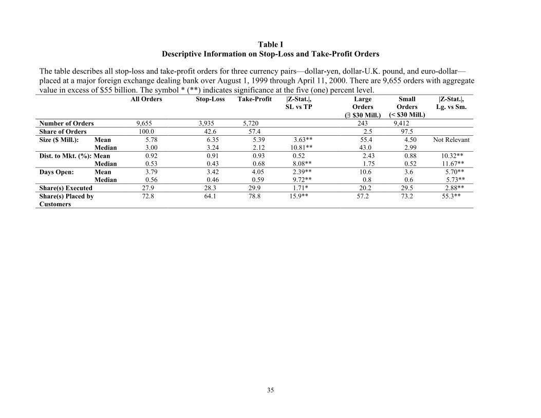
35
Table I Descriptive Information on Stop-Loss and Take-Profit Orders
The table describes all stop-loss and take-profit orders for three currency pairs—dollar-yen, dollar-U.K. pound, and euro-dollar— placed at a major foreign exchange dealing bank over August 1, 1999 through April 11, 2000. There are 9,655 orders with aggregate value in excess of $55 billion. The symbol * (**) indicates significance at the five (one) percent level. All Orders Stop-Loss Take-Profit |Z-Stat.|,
SL vs TP Large
Orders (∃ $30 Mill.)
Small Orders
(< $30 Mill.)
|Z-Stat.|, Lg. vs Sm.
Number of Orders 9,655 3,935 5,720 243 9,412 Share of Orders 100.0 42.6 57.4 2.5 97.5 Size ($ Mill.): Mean Median
5.78 3.00
6.35 3.24
5.39 2.12
3.63** 10.81**
55.4 43.0
4.50 2.99
Not Relevant
Dist. to Mkt. (%): Mean Median
0.92 0.53
0.91 0.43
0.93 0.68
0.52 8.08**
2.43 1.75
0.88 0.52
10.32** 11.67**
Days Open: Mean Median
3.79 0.56
3.42 0.46
4.05 0.59
2.39** 9.72**
10.6 0.8
3.6 0.6
5.70** 5.73**
Share(s) Executed 27.9 28.3 29.9 1.71* 20.2 29.5 2.88** Share(s) Placed by Customers
72.8 64.1 78.8 15.9** 57.2 73.2 55.3**
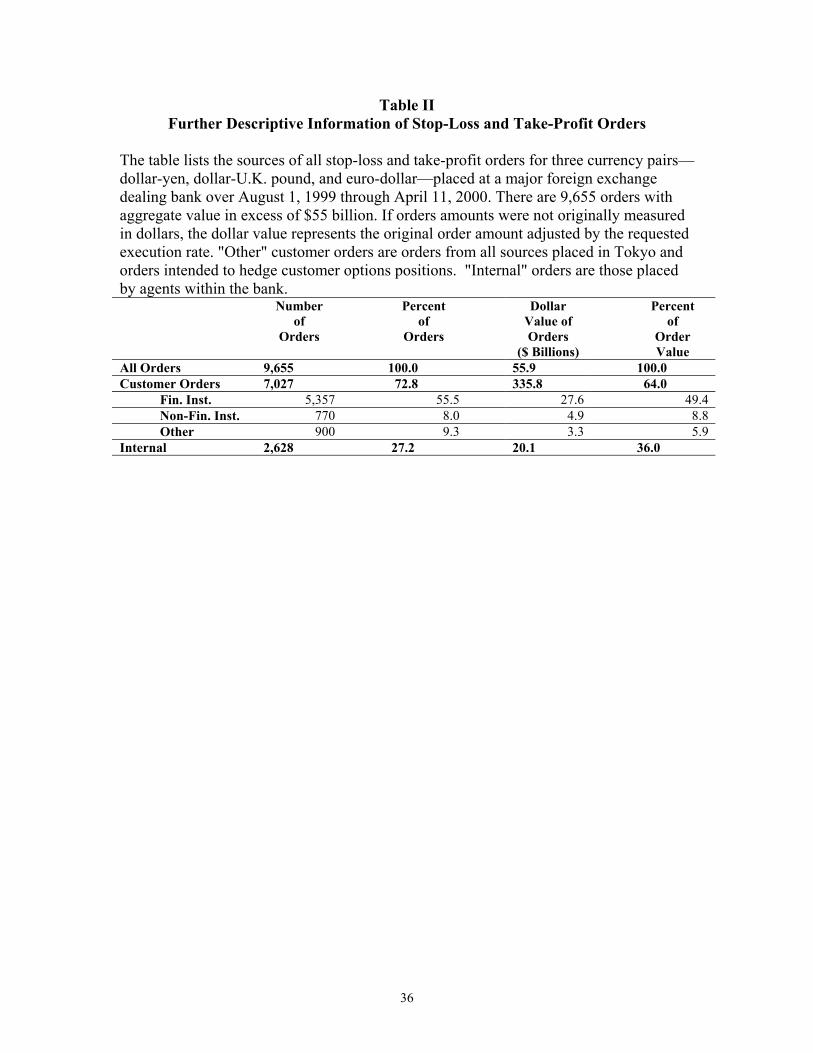
36
Table II Further Descriptive Information of Stop-Loss and Take-Profit Orders
The table lists the sources of all stop-loss and take-profit orders for three currency pairs—dollar-yen, dollar-U.K. pound, and euro-dollar—placed at a major foreign exchange dealing bank over August 1, 1999 through April 11, 2000. There are 9,655 orders with aggregate value in excess of $55 billion. If orders amounts were not originally measured in dollars, the dollar value represents the original order amount adjusted by the requested execution rate. "Other" customer orders are orders from all sources placed in Tokyo and orders intended to hedge customer options positions. "Internal" orders are those placed by agents within the bank. Number
of Orders
Percent of
Orders
Dollar Value of Orders
($ Billions)
Percent of
Order Value
All Orders 9,655 100.0 55.9 100.0 Customer Orders 7,027 72.8 335.8 64.0 Fin. Inst. 5,357 55.5 27.6 49.4 Non-Fin. Inst. 770 8.0 4.9 8.8 Other 900 9.3 3.3 5.9 Internal 2,628 27.2 20.1 36.0

37
Table III Requested Execution Rates Near Round Numbers
The table summarizes asymmetries in the distribution of requested execution rates near round numbers ending in 00 and 50 for price-contingent orders. Underlying data are all stop-loss and take-profit orders for three currency pairs–dollar-yen, dollar-U.K. pound, and euro-dollar—executed at a major bank over August 1, 1999 through April 11, 2000. There are 2,694 orders with aggregate value near $14.6 billion. For each entry, I take the percent of executed orders of each order type with requested execution rates ending in the indicated set of two-digit numbers, and sum them.
The marginal significance represents the likelihood of observing the actual difference between orders above and below the round number, under the following null hypothesis: Agents' preferences for round numbers are consistent with those in Figures 3 A to D, with a strongest preference for rates ending in (0) and successively weaker preferences for rates ending in (5), the set (2,3,7,8), and the set (1,4,6,9). However, agents' preferences do not differ significantly according to the digit preceding these numbers. For each type of order, 2,000 sums of 10 frequencies were generated, where each set included one observed frequency from rates ending in 0, one observed frequency from rates ending in 5, four observed frequencies from rates ending in 2, 3, 7, or 8, and four observed frequencies from rates ending in 1, 4, 6, or 9. From these, 1,000 differences were calculated and ranked. The ranked simulated differences provided marginal significance levels for the actual differences. Numbers in parentheses are marginal significance levels for the same tests applied to frequencies for all placed orders, weighted by order value. Stop-Loss Orders Take-Profit Orders Buy Sell Buy Sell At 00 4.4 4.3 8.2 11.8 Around 00 90-99 7.3 8.2 11.2 10.3 01-10 17.0 6.9 9.7 7.1 Difference 9.6 -1.3 -1.5 -3.2 Marg. Sig. 0.022 0.197 0.266 0.255 Around 50 40-49 4.8 15.0 9.1 8.3 51-60 17.0 6.7 7.6 7.6 Difference 12.2 -8.3 -1.5 -0.7 Marg. Sig. 0.005 0.000 0.264 0.461
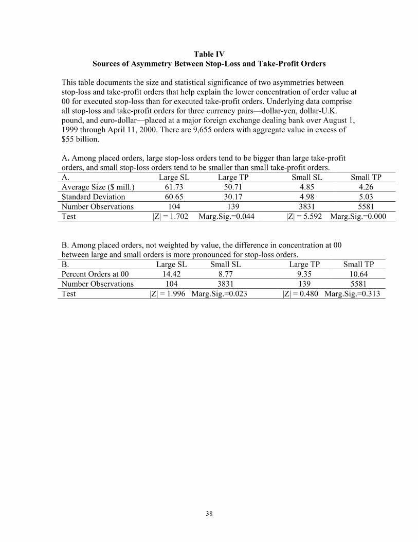
38
Table IV Sources of Asymmetry Between Stop-Loss and Take-Profit Orders
This table documents the size and statistical significance of two asymmetries between stop-loss and take-profit orders that help explain the lower concentration of order value at 00 for executed stop-loss than for executed take-profit orders. Underlying data comprise all stop-loss and take-profit orders for three currency pairs—dollar-yen, dollar-U.K. pound, and euro-dollar—placed at a major foreign exchange dealing bank over August 1, 1999 through April 11, 2000. There are 9,655 orders with aggregate value in excess of $55 billion. A. Among placed orders, large stop-loss orders tend to be bigger than large take-profit orders, and small stop-loss orders tend to be smaller than small take-profit orders. A. Large SL Large TP Small SL Small TP Average Size ($ mill.) 61.73 50.71 4.85 4.26 Standard Deviation 60.65 30.17 4.98 5.03 Number Observations 104 139 3831 5581 Test |Z| = 1.702 Marg.Sig.=0.044 |Z| = 5.592 Marg.Sig.=0.000 B. Among placed orders, not weighted by value, the difference in concentration at 00 between large and small orders is more pronounced for stop-loss orders. B. Large SL Small SL Large TP Small TP Percent Orders at 00 14.42 8.77 9.35 10.64 Number Observations 104 3831 139 5581 Test |Z| = 1.996 Marg.Sig.=0.023 |Z| = 0.480 Marg.Sig.=0.313
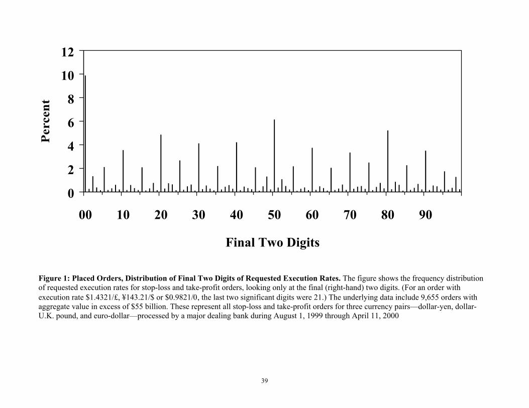
39
Figure 1: Placed Orders, Distribution of Final Two Digits of Requested Execution Rates. The figure shows the frequency distribution of requested execution rates for stop-loss and take-profit orders, looking only at the final (right-hand) two digits. (For an order with execution rate $1.4321/£, ¥143.21/$ or $0.9821/0, the last two significant digits were 21.) The underlying data include 9,655 orders with aggregate value in excess of $55 billion. These represent all stop-loss and take-profit orders for three currency pairs—dollar-yen, dollar-U.K. pound, and euro-dollar—processed by a major dealing bank during August 1, 1999 through April 11, 2000
0
2
4
6
8
10
12
00 10 20 30 40 50 60 70 80 90
Final Two Digits
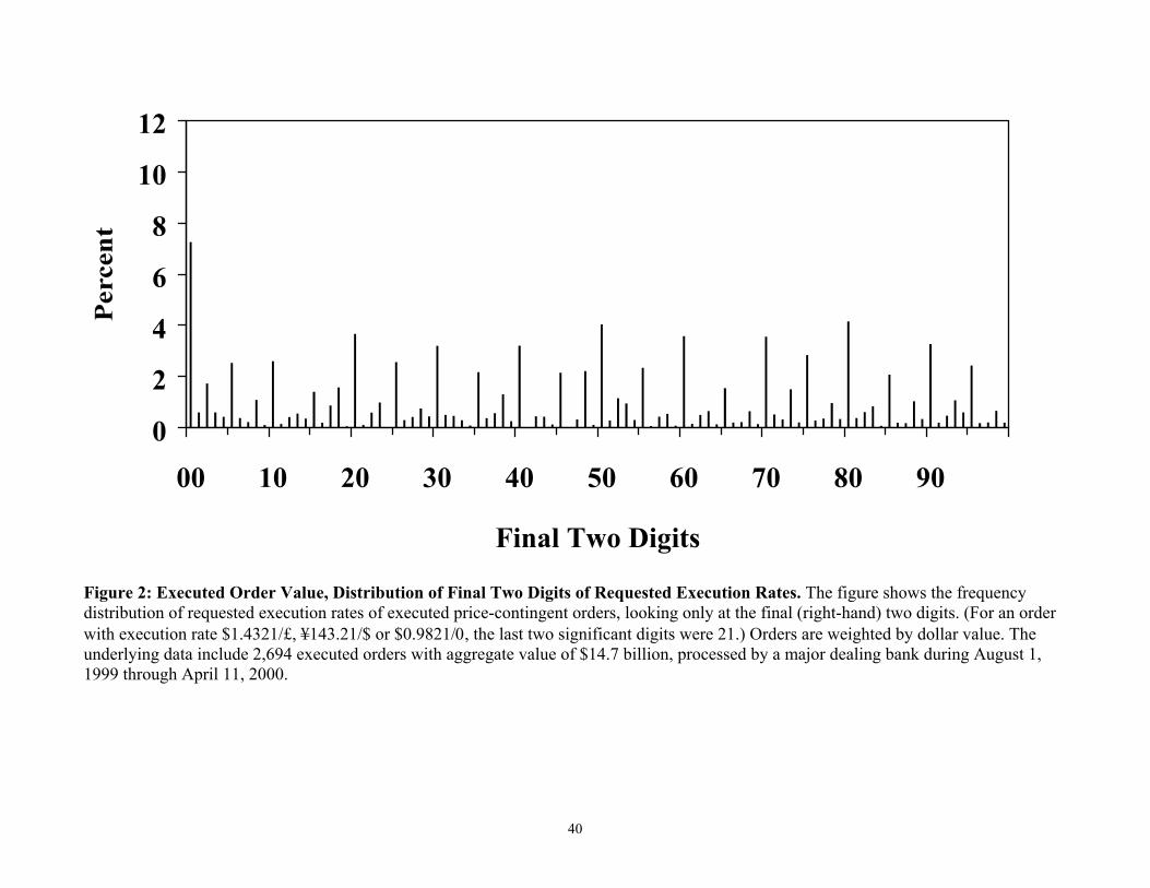
40
Figure 2: Executed Order Value, Distribution of Final Two Digits of Requested Execution Rates. The figure shows the frequency distribution of requested execution rates of executed price-contingent orders, looking only at the final (right-hand) two digits. (For an order with execution rate $1.4321/£, ¥143.21/$ or $0.9821/0, the last two significant digits were 21.) Orders are weighted by dollar value. The underlying data include 2,694 executed orders with aggregate value of $14.7 billion, processed by a major dealing bank during August 1, 1999 through April 11, 2000.
0
2
4
6
8
10
12
00 10 20 30 40 50 60 70 80 90
Final Two Digits
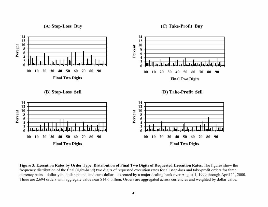
41
Figure 3: Execution Rates by Order Type, Distribution of Final Two Digits of Requested Execution Rates. The figures show the frequency distribution of the final (right-hand) two digits of requested execution rates for all stop-loss and take-profit orders for three currency pairs—dollar-yen, dollar-pound, and euro-dollar—executed by a major dealing bank over August 1, 1999 through April 11, 2000. There are 2,694 orders with aggregate value near $14.6 billion. Orders are aggregated across currencies and weighted by dollar value.
(A) Stop-Loss Buy
(B) Stop-Loss Sell
(C) Take-Profit Buy
(D) Take-Profit Sell
02468
101214
00 10 20 30 40 50 60 70 80 90
Final Two Digits
Perc
ent
02468
101214
00 10 20 30 40 50 60 70 80 90
Final Two Digits
Perc
ent
02468
101214
00 10 20 30 40 50 60 70 80 90
Final Two Digits
Perc
ent
02468
101214
00 10 20 30 40 50 60 70 80 90
Final Two Digits
Perc
ent
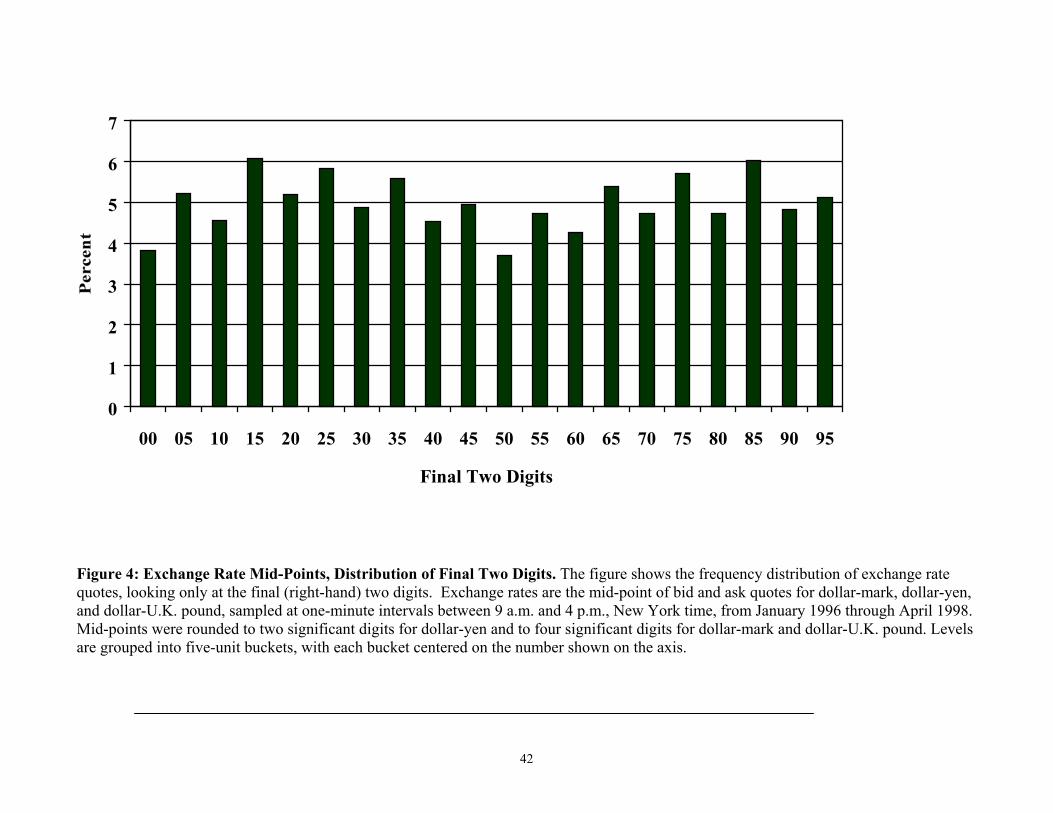
42
Figure 4: Exchange Rate Mid-Points, Distribution of Final Two Digits. The figure shows the frequency distribution of exchange rate quotes, looking only at the final (right-hand) two digits. Exchange rates are the mid-point of bid and ask quotes for dollar-mark, dollar-yen, and dollar-U.K. pound, sampled at one-minute intervals between 9 a.m. and 4 p.m., New York time, from January 1996 through April 1998. Mid-points were rounded to two significant digits for dollar-yen and to four significant digits for dollar-mark and dollar-U.K. pound. Levels are grouped into five-unit buckets, with each bucket centered on the number shown on the axis.
0
1
2
3
4
5
6
7
00 05 10 15 20 25 30 35 40 45 50 55 60 65 70 75 80 85 90 95
Final Two Digits
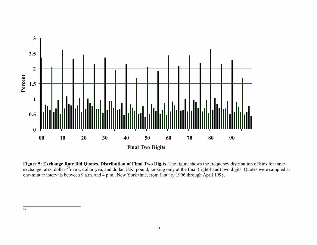
43
Figure 5: Exchange Rate Bid Quotes, Distribution of Final Two Digits. The figure shows the frequency distribution of bids for three exchange rates, dollar-29mark, dollar-yen, and dollar-U.K. pound, looking only at the final (right-hand) two digits. Quotes were sampled at one-minute intervals between 9 a.m. and 4 p.m., New York time, from January 1996 through April 1998.
29
0
0.5
1
1.5
2
2.5
3
00 10 20 30 40 50 60 70 80 90
Final Two Digits
Perc
ent
