Cross-Border Financial Surveillance: A Network Perspective

Marco A. Espinosa-Vega and Juan Solé

WP/10/105

© 2010 International Monetary Fund WP/10/105 IMF Working Paper Monetary and Capital Markets

Cross-Border Financial Surveillance: A Network Perspective

Prepared by Marco Espinosa-Vega and Juan Solé1

Authorized for distribution by Laura Kodres

April 2010

Abstract

This Working Paper should not be reported as representing the views of the IMF. The views expressed in this Working Paper are those of the author(s) and do not necessarily represent those of the IMF or IMF policy. Working Papers describe research in progress by the author(s) and are published to elicit comments and to further debate.

Effective cross-border financial surveillance requires the monitoring of direct and indirect systemic linkages. This paper illustrates how network analysis could make a significant contribution in this regard by simulating different credit and funding shocks to the banking systems of a number of selected countries. After that, we show that the inclusion of risk transfers could modify the risk profile of entire financial systems, and thus an enriched simulation algorithm able to account for risk transfers is proposed. Finally, we discuss how some of the limitations of our simulations are a reflection of existing information and data gaps, and thus view these shortcomings as a call to improve the collection and analysis of data on cross-border financial exposures. JEL Classification Numbers: F34, F35, G21 Keywords: Financial Surveillance, Network Analysis, Cross-Border Financial Linkages Author’s E-Mail Address: mespinosa@imf.org, jsole@imf.org

1 We are grateful to the following for their helpful comments and suggestions: Rama Cont, Sean Craig, Kay Giesecke, Kristian Hartelius, John Kiff, Laura Kodres, Lavan Mahadeva, Patrick McGuire, Diego Rodriguez-Palazuela, Carolynne Spackman (who also provided excellent research assistance), Thierry Tressel, Christian Upper, Götz von Peter, and seminar participants at the IMF, the Bank for International Settlements, the European Central Bank, the Bank of Japan, the Japanese Financial Services Agency, the Japanese Center for Economic Research, Bank Negara Malaysia, the South Africa Reserve Bank, the “Liquidity 2009 Conference” organized by E-MiD (Italy), and the 1st IMF Roundtable to Enhance Collaboration on Financial Stability Analysis. Graham Colin-Jones provided superb editorial assistance. We are also indebted to the BIS for the provision of data. All errors and omissions are the authors’.

2

Contents Page

I. Introduction ............................................................................................................................3

II. A Simple Interbank Exposure Model ....................................................................................4 A. Network Simulations of Credit and Liquidity Shocks ..............................................5 B. The Simulation Algorithms .......................................................................................8 C. The Data ....................................................................................................................9

III. Simulation Results .............................................................................................................12 A. Simulation 1: The Transmission of a Credit Shock ................................................12 B. Simulation 2: The Transmission of a Credit-plus-Funding Shock ..........................16 C. Simulations 3 and 4: Transmission of Shocks in the Presence of Risk Transfers ..18

IV. Concluding Remarks .........................................................................................................21

References ................................................................................................................................23

Appendix I: Comparing Results Based on the IBB and the URB Datasets .............................26 Tables 1. Results for Simulation 1 (Credit Channel)...........................................................................13 2. Country-by-Country Capital Impairment ............................................................................15 3. Results for Simulation 2 (Credit and Funding Channel) .....................................................17 4. Country-by-Country Capital Impairment (Credit and Funding Channel) ...........................18 Figures 1. Network Analysis based on Interbank Exposures .................................................................4 2. Effect of a Credit Shock on a Bank’s Balance Sheet .............................................................5 3. Effect of Credit and Funding Shock on a Bank’s Balance Sheet ..........................................7 4. Cross-Border Claims on Immediate Borrower Basis and Ultimate Risk Basis ...................10 6. Number of Induced Failures ................................................................................................14 7. Country-by-Country Vulnerability Level ............................................................................15 8. Contagion Path Triggered by the U.K. Failure Under the Credit Shock Scenario ..............16 9. Number of Induced Failures—Uniform Distribution ..........................................................19 10. Country-by-Country Vulnerability Level—Uniform Distribution ....................................19 11. Number of Induced Failures—Biased Distribution ...........................................................20 12. Country-by-Country Vulnerability Level—Biased Distribution .......................................20

3

I. INTRODUCTION

Effective financial system surveillance requires the monitoring of direct and indirect financial linkages, whose disruption could have important implications for the stability of the entire financial system. Indeed, the recent financial crisis has underscored the need to go beyond the analysis of individual institutions’ soundness and assess whether the linkages across institutions may have systemic implications. Furthermore, it has become clear that, due to these financial interconnections, during stress events, even actions geared to enhance the soundness of a particular institution may undermine the stability of other institutions. Consider, for instance, the depiction of the Northern Rock case by Morris and Shin (2008): “a prudent shedding of exposures from the point of view of Bank 2 is a run from the point of view of Bank 1. Arguably, this type of run is what happened to the U.K. bank Northern Rock, which failed in 2007” (italics added).2

Therefore, policymakers and regulators worldwide have become increasingly aware of the importance of proactively tracking potential systemic linkages. As pointed out by, for instance, Allen and Babus (2007), network analysis is a natural candidate to aid in this challenge, as it allows regulators and policymakers to assess externalities to the rest of the financial system, by tracking the rounds of spillovers likely to arise from direct financial linkages. 3

This paper shows how network analysis can be used for cross-border financial sector surveillance by simulating different credit and funding shocks to the banking systems of a number of selected countries. In addition, the paper illustrates how the inclusion of risk transfers (or contingent exposures) can alter the risk profile of an entire financial system. The basis of our analysis is the set of cross-country interbank exposures (including gross lending and borrowing and risk transfers) estimates of a selected number of countries that report their banking data to the BIS. For purely illustrative purposes we use BIS cross-country data. Our goal in carrying out this analysis is not to make specific pronouncements about particular countries, but to illustrate the techniques described in the paper as a useful tool for (macro-) financial surveillance.

2 While the quote rightly points to the liquidity squeeze suffered by Northern Rock, it is important to note that the main source of the squeeze came from the wholesale market and not the interbank market. 3 See Upper (2007) for an insightful survey of the network literature. While most of the network literature that will be referenced in this chapter is of an applied nature, see Allen and Gale (2000) and Freixas et al. (2000) for some theoretical underpinnings to the network approach. In addition, Nier et al. (2007) apply network theory to study contagion risk in simulated banking systems. There are also a number of papers that have focused on domestic banking systems—e.g., Boss et al. (2004) and Elsinger et al. (2006) for Austria; Furfine (2003) for the United States; Márquez, and Martínez (2008) for Mexico; Memmel and Stein (2008) and Upper and Worms (2004) for Germany; Sheldon and Maurer (1998) and Müller (2006) for Switzerland; and Wells (2004) for the United Kingdom, among others. Finally, see Chan-Lau, Espinosa, Giesecke, and Solé (2009) for a cross-border application.

4

Among other things, the paper tracks the systemic impact unleashed by the execution of cross-border interbank risk transfers following a credit event. The algorithm designed to track the domino effects triggered by hypothetical credit and funding shocks to each banking system in our sample is illustrated in Figure 1.

Figure 1: Network Analysis based on Interbank Exposures

Source: Márquez and Martínez (2008) and authors.

The rest of the paper is organized as follows. Section II provides a detailed explanation of the methodology for the simulations and the data. Section III presents the results of our simulations. Section IV concludes, while Appendix I presents some additional results obtained with an additional dataset.

II. A SIMPLE INTERBANK EXPOSURE MODEL

The point of departure for our analysis is a stylized bank balance sheet that highlights the role of cross-border interbank exposures. The first set of simulations (simulation 1) examines the domino effects triggered by the default of a banking system’s interbank obligations—we call this a credit shock. The second set of simulations (simulation 2) looks at the effects of a credit-plus-funding event, where the default of an institution also leads to a liquidity squeeze for those institutions funded by the defaulting institution (i.e., the credit shock is compounded by a funding shock and associated fire sale losses). After this, we look at the effects of incorporating risk transfers into our analysis (simulations 3 and 4).

5

A. Network Simulations of Credit and Liquidity Shocks

To assess the potential systemic implications of interbank linkages, the paper considers a network of N institutions. The point of departure is the following stylized balance sheet identity for bank i: (1) ji i i i i ijj j

x a k b d x+ = + + +∑ ∑ ,

where jix stands for bank i loans to bank j, ia stands for bank i’s other assets, ik stands for bank i’s capital, ib are long-term and short-term borrowing (excluding interbank loans),

id stands for deposits, and ijx stands for bank i borrowing from bank j. Transmission of Credit Shocks To analyze the effects of a credit shock, the paper simulates the individual default of each one of the 18 banking systems in the network, for different assumptions of loss given default (denoted by the parameter λ), it is assumed that banking system i’s capital absorbs the losses on impact, and then we track the sequence of defaults triggered by this event. For instance, after taking into account the initial credit loss stemming from the default of, say, institution h, the baseline balance sheet identity of bank i becomes:

(2) ( ) ∑+++−=−+∑+ ≠ j ijiihiihihj jii xdbxkxxa λλ)1( ,

and bank i is said to fail if its capital is insufficient to fully cover its losses (i.e., if 0i hik xλ− < ). These losses are depicted in light gray in Figure 2.4

Figure 2: Effect of a Credit Shock on a Bank’s Balance Sheet

4 Subsequent rounds in the algorithm take into account the losses stemming from all failed institutions up to that point.

6

Transmission of Credit-plus-Funding Shocks The extent to which a bank is able to replace an unforeseen withdrawal of interbank funding will depend on money market liquidity conditions. During the 2007–09 crisis, for instance, we saw a gradual freezing of money markets that started with financial institutions becoming reluctant to roll over their funding of counterparties whose portfolios or business models were perceived to be similar to those of seemingly weak institutions.5

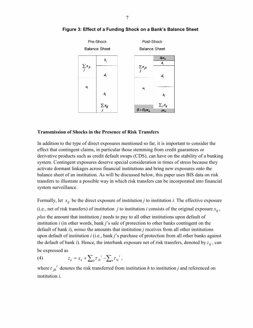
When liquidity is tight and in the absence of alternative sources of funding, a bank may be forced to sell part of its assets in order to restore its balance sheet identity. We study the situation where, as in the 2007–09 crisis, a bank is able to replace only a fraction of the lost funding and its assets trade at a discount (i.e., their market value is less than their book value). We exclude the possibility of institutions raising new capital, and assume that the loss induced by a funding shortfall is absorbed by the bank’s capital (Figure 3). Therefore, a bank’s vulnerability not only stems from its direct credit exposures to other institutions, but also from its inability to roll over (part of) its funding in the interbank market, and thus having to sell assets at a discount in order to re-establish its balance sheet identity.

In terms of our stylized model, it is assumed that institutions are unable to replace all the funding previously granted by the defaulted institutions, which, in turn, triggers a fire sale of assets. Thus, we study the situation where bank i is able to replace only a fraction )1( ρ− of the lost funding from bank h, and its assets trade at a discount, so that bank i is forced to sell assets worth ihxρδ )1( + in book value terms.6

ihxδρ The funding-shortfall induced loss, , is absorbed by bank i’s capital (Figure 3), and thus the new balance sheet identity for institution i is given by

(3) ( ) ( ) ihj ijiiihiihj jii xxdbxkxxa ρδρρδ −∑+++−=+−∑+ 1 .

5 Indirect linkages among financial institutions may arise when banks hold the same type of asset in their balance sheets. These linkages can represent an important source of systemic risk, as the forced sale of assets by some institutions may trigger a decline in the market value of the other institutions’ portfolios. Models with this type of portfolio linkages can be found, for instance, in Cifuentes et al (2005), Elsinger at al. (2006), Lagunoff and Schreft (2001), and Vries (2005). In addition, Furfine (2003), Nier et al. (2007) and Müller (2006) also analyze liquidity shocks.

6 An alternative way to see this is the following. Let xρ be the amount of funding that cannot be replaced. Let 1p be the current market price for assets and let y be the quantity of assets sold. That is, xyp ρ=1 . Suppose that

these assets had been bought at a higher price 0p , thus )1(01 δρρ +≡<= xypypx . Hence, it is possible to find

a relationship between the parameter δ and the change in asset prices: 110 /)( ppp −=δ , i.e., δ is a parameter reflecting the degree of distress in asset markets. Higher δ reflects higher distress in markets.

7

Figure 3: Effect of a Funding Shock on a Bank’s Balance Sheet

Transmission of Shocks in the Presence of Risk Transfers In addition to the type of direct exposures mentioned so far, it is important to consider the effect that contingent claims, in particular those stemming from credit guarantees or derivative products such as credit default swaps (CDS), can have on the stability of a banking system. Contingent exposures deserve special consideration in times of stress because they activate dormant linkages across financial institutions and bring new exposures onto the balance sheet of an institution. As will be discussed below, this paper uses BIS data on risk transfers to illustrate a possible way in which risk transfers can be incorporated into financial system surveillance. Formally, let ijx be the direct exposure of institution j to institution i. The effective exposure

(i.e., net of risk transfers) of institution j to institution i consists of the original exposure ijx , plus the amount that institution j needs to pay to all other institutions upon default of institution i (in other words, bank j’s sale of protection to other banks contingent on the default of bank i), minus the amounts that institution j receives from all other institutions upon default of institution i (i.e., bank j’s purchase of protection from all other banks against the default of bank i). Hence, the interbank exposure net of risk transfers, denoted by ijz , can be expressed as (4) ∑∑ −+=

hi

hjhi

jhijij xz ττ ,

where ijhτ denotes the risk transferred from institution h to institution j and referenced on

institution i.

8

B. The Simulation Algorithms

A. The algorithm without risk transfers For each of the simulations, we programmed a Matlab network algorithm of a system consisting of N nodes (each node representing a banking system) and with a structure of inter-node (or interbank) loans represented by the NN × matrix, X, with a generic element denoted by ijx —note that these loans are direct exposures across nodes. Let tF be the set of failed institutions and let tNF be the set of not-failed institutions in round t of the simulations. To initialize the credit shock simulation (simulation 1), assume that institution h fails at t=0, and thus a fraction λ of its debts to the rest of institutions will not be repaid. Then, for each one of the not-failed institutions, tNFj∈ , the algorithm checks whether the amount of losses suffered by that institution is larger than the amount of capital of that particular institution. If that is the case, then that institution is also driven to bankruptcy. That is,

(5) 1 : toodefaults if +∈

∈⇒>∑ tjtFh

hj Fjjkxλ

The algorithm is said to converge once there are no further failures: that is, 1+= tt FF . For the credit-plus-funding shock simulations (simulation 2), the previous shock is compounded by the funding-shortfall induced loss, ihxδρ . That is, at each stage of the simulation, an institution’s capital may be negatively affected by the asset fire sale (recall Figure 3), and hence the default condition is given by

(6) 1 : toodefaults if +∈∈

∈⇒>∑+∑ tjtFh

jhtFh

hj Fjjkxx δρλ .

B. The algorithm with risk transfers We also programmed an algorithm that takes into account the effects of risk transfers on the transmission of both the credit and the credit-plus-funding shocks through the network (simulations 3 and 4, respectively). For this, the previous algorithm was modified so that the default condition for the credit shock becomes

(7) 1 : toodefaults if +∈ ∈∈ ∈∈

∈⇒>∑ ∑+∑ ∑−∑ tjtFh tNFi

hji

tFh tNFi

hij

tFhhj Fjjkx λτθλτλ .

The default condition for the credit-plus-funding shock becomes (8) j

tFh tNFi

hji

tFh tNFi

hij

tFhjh

tFhhj kxx >∑ ∑+∑ ∑−∑+∑

∈ ∈∈ ∈∈∈λτθλτδρλ if ,

1 : toodefaults +∈⇒ tFjj , where the parameter θ captures the fraction of risk transfers that have not been provisioned for. Note that, in the last two equations above, outward and inward transfers are treated slightly differently: while both transfers are multiplied byλ , inward transfers are also

9

multiplied by the parameterθ . This is to recognize the possibility that institutions may make provisions for those risk transfers that they take onto their balance sheets. 7

After the default of an institution, the inward risk transfers of that institution are set to zero, since the defaulted institution will not be able to honor the guarantees it has extended. In terms of the notation above, this amounts to setting 0=i

hjτ , for all j, after the default of bank

h. For instance, if 5=ihjτ billion USD, this implies that if institution i defaults, then h needs

to make a transfer of $5 billion to institution j.

C. The Data8

To illustrate the use of network analysis for cross-border financial surveillance, we focused on cross-country bilateral exposures at end-December 2007, published in the BIS’ International Consolidated Banking Statistics database. The BIS compiles these data in two formats: (i) immediate borrower basis (IBB) and (ii) ultimate risk basis (URB). While both datasets consolidate the exposures of lenders’ foreign offices (i.e., subsidiaries and branches) into lenders’ head offices, the URB dataset also consolidates by residency of the ultimate obligor (i.e., the party that is ultimately responsible for the obligation in case the immediate borrower defaults) and includes net risk transfers.

9

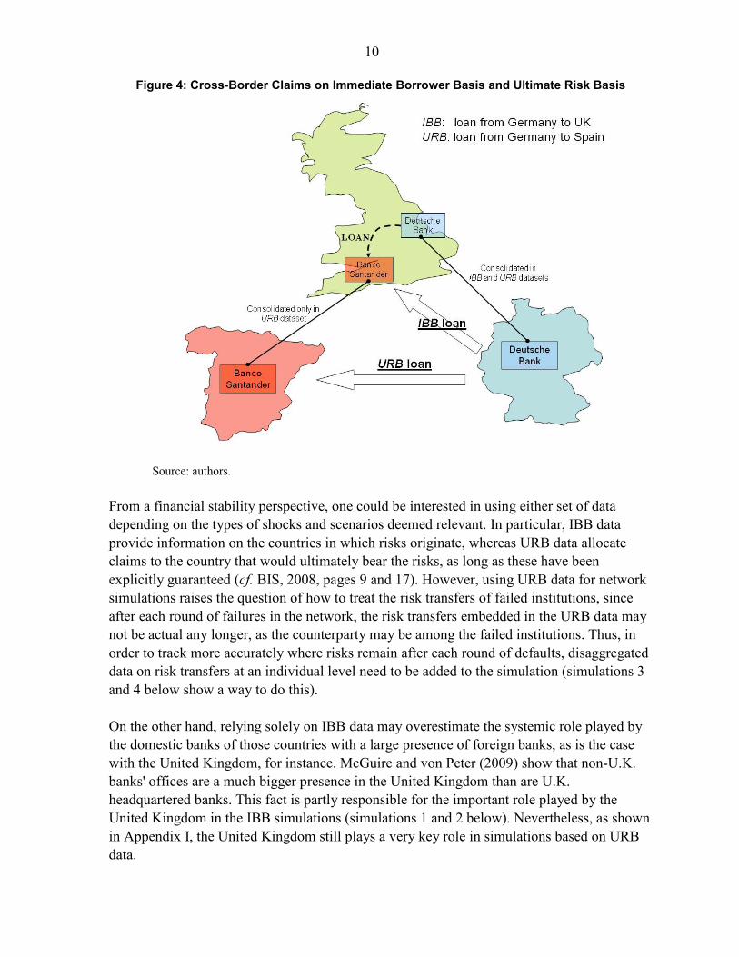
Thus, for example, on an immediate borrower basis, a loan from Deutsche Bank's subsidiary in London to Banco Santander's subsidiary in London would appear as a loan from Germany to the United Kingdom in the IBB statistics (Figure 4). On the other hand, on an ultimate risk basis, the borrower's balance sheet is also consolidated (as long as the parent entity explicitly guarantees the claim), and thus, the same loan described above would be accounted for as a loan from Germany to Spain.

7 For comparison purposes, and given the lack of reliable estimates for its empirical value, this parameter was arbitrarily set equal to the loss-given-default parameter, λθ = , in order not to bias the results in favor of or against the simulations that include risk transfers: simulations with λθ < would produce less defaults and vice versa. Factors that in practice would affect the numerical value of this parameter include: the fraction of risk transfers that have been provisioned for or the cheapest-to-deliver option available to the protection seller at the time a transfer needs to be made.

8 We are indebted to Patrick McGuire and Götz von Peter for extensive discussions on the BIS statistics.

9 See McGuire and Wooldridge (2005) and BIS (2008) for a detailed description of these data, and McGuire and Tarashev (2008) for applications of the BIS statistics to monitor the international banking system. Hattori and Suba (2001) also use BIS data to study the network topology of the international banking system from a historical perspective. However, their study does not assess contagion patterns.

10

Figure 4: Cross-Border Claims on Immediate Borrower Basis and Ultimate Risk Basis

Source: authors.

From a financial stability perspective, one could be interested in using either set of data depending on the types of shocks and scenarios deemed relevant. In particular, IBB data provide information on the countries in which risks originate, whereas URB data allocate claims to the country that would ultimately bear the risks, as long as these have been explicitly guaranteed (cf. BIS, 2008, pages 9 and 17). However, using URB data for network simulations raises the question of how to treat the risk transfers of failed institutions, since after each round of failures in the network, the risk transfers embedded in the URB data may not be actual any longer, as the counterparty may be among the failed institutions. Thus, in order to track more accurately where risks remain after each round of defaults, disaggregated data on risk transfers at an individual level need to be added to the simulation (simulations 3 and 4 below show a way to do this). On the other hand, relying solely on IBB data may overestimate the systemic role played by the domestic banks of those countries with a large presence of foreign banks, as is the case with the United Kingdom, for instance. McGuire and von Peter (2009) show that non-U.K. banks' offices are a much bigger presence in the United Kingdom than are U.K. headquartered banks. This fact is partly responsible for the important role played by the United Kingdom in the IBB simulations (simulations 1 and 2 below). Nevertheless, as shown in Appendix I, the United Kingdom still plays a very key role in simulations based on URB data.

11

From an operational standpoint, since both datasets have limitations, our inclination would be to conduct simulations using both datasets and compare results. For expository purposes, however, and given that our simulations including risk transfers build from data on an immediate borrower basis, we present first the results based on IBB data, and relegate the results obtained using URB data to Appendix I.10

We also obtained data on cross-border risk transfers from the BIS. These data represent inward and outward transfers of risks by reporting banks, and include credit guarantees and commitments, collateral, and credit derivatives in the banking book (cf. BIS 2008, page 16).11

Unfortunately, it was not possible to obtain a further disaggregation, either by sector and nationality of the referenced entities (i.e., the entities on whose performance the risk transfer is contingent) or by sector of the party receiving the risk transfer.

Therefore, we had to assume a distribution of risk transfers across countries of residence of the referenced institution, and that all risk transfers were interbank transfers. A generalized practice in the literature is to use maximum entropy to generate the unknown distribution. However, this procedure would be akin to assuming a uniform distribution of risk transfers across (referenced) countries, which would, in turn, spread the risk to the maximum amount possible and thus probably give an overly benign picture of systemic risk in the network. Alternatively, and in order to make a (perhaps more plausible) approximation of the distribution of risk transfers, we assumed that the distribution of referenced entities is the same as the distribution of direct credit exposures (simulation 3). As a robustness check, we also conducted an additional set of simulations assuming a concentrated distribution of risk transfers for some countries (simulation 4). Data on country specific bank capital at end-December 2007 were obtained from Bankscope. To match as closesly as possible the number and type of banks in both datasets (i.e., BIS and Bankscope), we gathered data from only commercial and investment banks in Bankscope, excluding smaller entities (such as cooperative banks and savings banks) which, arguably, are less likely to engage in international transactions.

10 There is another difference between the IBB and the URB datasets that deserves mention: the sectoral split (e.g., banks vs. other sectors) is not consistent across the two datasets. In the IBB data, the sectoral split is only available for international claims (cross-border claims plus local claims in foreign currency), whereas there is no information on the sectoral split for local claims in local currency. In consequence, we applied the same sectoral fraction available for international claims to local claims in local currency. In contrast, in the URB data, the sectoral split applies to total foreign claims (equal to international plus local claims in local currency).

11 The BIS defines credit guarantees as contingent liabilities arising from an obligation to pay to a third-party when a client fails to perform a contractual obligation; credit commitments are irrevocable obligations to extend credit at the request of a borrower (cf. McGuire and Tarashev, 2008).

12

Finally, the list of the 18 countries analyzed were Australia, Austria, Belgium, Canada, Finland, France, Germany, Greece, Ireland, Italy, Japan, Netherlands, Portugal, Spain, Sweden, Switzerland, the United Kingdom, and the United States. Before proceeding to the description of our simulation results, we would like to reiterate that due to the data constraints just described, the results of the paper should be seen as merely illustrative of the potential of network analysis as a tool for cross-border financial surveillance.

III. SIMULATION RESULTS

We begin this next section by studying how shocks to a country’s resident financial institutions unravel throughout the network before one considers risk transfers (simulations 1 and 2). That is, we track shocks to financial institutions that are incorporated and operate in a given jurisdiction regardless of the residency of the parent company. Or to put it in terms of our example above, British regulators would be interested in tracking shocks not only to British banks, but also to the subsidiaries of foreign entities operating in the United Kingdom; hence, a shock to Santander’s subsidiary in London would be important to track. After that, we present a second set of simulations that incorporate off-balance sheet data on risk transfers (simulations 3 and 4). Due to the lack of granularity of the data, our analysis is subject to a number of caveats. In particular, it is probably unrealistic to view the entire external sector of a country’s banking system as suffering a shock large enough to cause the entire banking system of another country to fail. Also, these data only cover a subset of bank exposures, namely direct credit exposures, and do not include OTC derivatives, specifically CDS contracts. However, our study provides a compelling illustration of the type of surveillance analysis that can be extracted from network analysis, including the identification of systemic and vulnerable institutions, as well as the detection of data gaps for the identification of potentially systemic exposures.

A. Simulation 1: The Transmission of a Credit Shock

The first simulation focuses on the transmission of a pure credit shock, thus assuming that institutions are able to roll over their funding sources and do not need to resort to fire sales of assets. 12 The credit shocks we analyze consist of the hypothetical default of a banking system’s debts to foreign banks.13

12 The simulations assume that the loss-given-default parameter equals 100 percent on impact. That is, when the credit event first materializes, banks are unable to recover any of their loans, as it takes time for secondary (and distress-debt) markets to price recently defaulted instruments. Thus, the simulation results should be interpreted as the on-impact transmission of systemic instability. In a similar vein, Wells (2004) argues that network studies should consider higher loss-given-default estimates than typically assumed, as banks tend to face substantial uncertainty over recovery rates in the short run.

The results of this simulation are reported in Table 1. Not

13 Admittedly, this is an extreme scenario but is considered for illustrative purposes.

13

surprisingly, what immediately emerges is that the U.K. and the U.S. banking systems are systemic players. Specifically, as of December 2007, the default of the U.K. and the U.S. systems would have led to losses—after all contagion rounds—of 45 and 96 percent, respectively, of the combined capital in our universe of banking systems. The second and third columns in Table 1 indicate the number of induced failures and the number of contagion rounds (the aftershocks) triggered by each hypothetical failure. The two countries that induce the highest number of contagion rounds are the United Kingdom and the United States (Figure 5). The failure of the U.K. banking system would trigger severe distress in 11 additional banking systems in three rounds of contagion. Similarly, the failure of the U.S. banking system would trigger the failure of 14 additional banking systems in three rounds of contagion.

Table 1. Results for Simulation 1 (Credit Channel)

CountryFailed Capital

(% of total capital)

Induced Failures

Contagion Rounds

Absolute Hazard 1/ Hazard Rate 2/

Australia 2.57 -- -- -- 0.0Austria 0.90 -- -- 3 17.6Belgium 1.62 -- -- 4 23.5Canada 3.49 -- -- 1 5.9Finland 1.24 1 1 -- 0.0France 6.59 -- -- 3 17.6Germany 3.65 -- -- 3 17.6Greece 0.73 -- -- -- 0.0Ireland 2.29 -- -- 2 11.8Italy 24.57 7 3 2 11.8Japan 15.02 1 1 1 5.9Netherlands 5.64 1 1 3 17.6Portugal 0.49 -- -- 2 11.8Spain 4.19 -- -- 2 11.8Sweden 0.77 -- -- 4 23.5Switzerland 1.78 -- -- 4 23.5United Kingdom 45.03 11 3 1 5.9United States 96.23 14 3 -- 0.0

1/ Number of simulations in which that particular country fails.2/ Percentage of failures as a percent of the number of simulations conducted.

14

Figure 5. Number of Induced Failures

0

2

4

6

8

10

12

14

16

18

Finland France Germany Italy Netherlands Japan Spain United Kingdom

United States

Credit Channel

Credit and Funding Channel

Note: the figure shows the number of countries whose banking systems would fail as a result of the initial failure of each country (e.g., the initial failure of France would induce no failure under the credit shock scenario and 14failures under the credit-plus-funding shock scenario).

It is important to emphasize that network analysis is useful not only in identifying potential failures, but also in estimating the amount of impaired capital after all aftershocks have taken place. In other words, even when domino effects do not lead to systemic failures, network analysis provides a measure of the degree to which a financial system will be weakened by the transmission of financial distress across institutions (Table 2). For instance, the failure of Germany would produce a capital loss to Greek banks of only 1.4 percent of their initial capital, whereas the loss for Ireland would amount to 38 percent of initial capital. In addition, this analysis facilitates not only the identification of institutions/systems whose stress poses systemic risks, but also “vulnerable” systems. For example, while the United Kingdom and the United States were identified as the most systemic systems (i.e., triggering the largest number of contagion rounds and the highest capital losses), Belgium, Sweden, and Switzerland appear the most vulnerable banking systems, exhibiting the highest hazard rates in the sample (Table 1). In other words, the banking systems of these countries are severely affected in four out of the 17 simulations in which they were not the trigger country (Figure 6). This is not to say that a crisis in these countries is imminent and/or unavoidable. The point is that this type of analysis allows for the identification of the weakest points within the network.

15

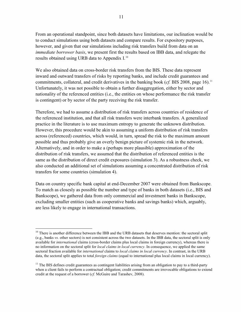
Table 2. Country-by-Country Capital Impairment (Credit Channel)

Australia Austria Belgium Canada Finland France Germany Greece Ireland Italy Japan Nether. Portugal Spain Sweden Switzer. U.K. U.S.Trigger Country:Australia -3.6 -5.7 -4.6 0.0 -12.3 -20.1 0.0 -4.0 -0.4 -4.8 -22.9 -1.1 -0.9 -5.2 -27.7 -13.6 -0.7Austria 0.0 -8.3 -0.5 -0.5 -5.6 -35.5 -0.7 -6.5 -23.4 -0.6 -2.8 -1.7 -0.8 -3.2 -14.9 -0.9 -0.1Belgium -0.7 -5.6 -1.1 -0.7 -23.6 -17.2 -1.1 -3.3 -3.8 -2.7 -43.5 -3.9 -4.3 -6.1 -20.4 -3.9 -0.2Canada 0.0 -1.9 -4.1 0.0 -5.9 -13.2 -0.1 -5.2 -0.4 -3.7 -10.3 -0.3 -0.6 -2.8 -20.8 0.0 -1.0Finland -0.1 -3.4 -4.6 -0.9 -5.4 -18.1 -0.1 -3.3 -1.1 -1.5 -5.0 -1.3 -1.3 Full -10.7 -2.4 -0.2France -2.9 -12.2 -81.6 -2.9 -3.3 -70.3 -1.5 -14.2 -11.8 -8.9 -43.8 -12.1 -15.5 -14.0 -71.4 -22.3 -1.0Germany 0.0 -70.2 -52.6 -3.8 -10.1 -54.2 -1.4 -38.0 -74.8 -11.1 -50.0 -15.6 -12.8 -96.1 -86.8 -11.0 -1.4Greece 0.0 -6.9 -9.2 -0.2 -1.2 -13.6 -12.8 -4.2 -1.6 -0.6 -5.3 -13.8 -0.2 -0.6 -45.6 -1.2 -0.1Ireland -2.0 -11.3 -62.2 -4.6 -2.7 -20.9 -62.4 -1.0 -5.8 -3.3 -12.5 -8.9 -5.9 -7.3 -28.3 -17.5 -0.5Italy -6.1 Full Full -12.7 -19.6 Full Full -6.7 -98.2 -34.5 Full -63.8 -58.2 Full Full -58.5 -4.5Japan -1.4 -11.7 -10.2 -2.0 0.0 -48.8 -47.9 -0.4 -7.7 -3.6 -19.1 -7.2 -1.5 -4.7 Full -12.4 -2.0Nether. -2.4 -25.4 Full -3.3 -3.7 -53.2 -69.8 -2.3 -11.1 -10.2 -7.3 -15.6 -18.1 -23.2 -60.1 -13.0 -1.1Portugal 0.0 -2.7 -6.0 -0.2 -0.3 -7.2 -14.5 0.0 -3.3 -1.5 -0.2 -3.9 -19.2 -0.7 -3.6 -1.4 -0.1Spain -0.6 -9.4 -30.3 -1.2 -2.7 -43.1 -89.9 -0.2 -16.9 -5.0 -2.3 -34.4 -59.1 -12.5 -18.0 -10.3 -0.6Sweden 0.0 -1.9 -2.6 -0.6 0.0 -3.5 -13.1 0.0 -3.3 -0.5 -1.1 -3.8 -1.1 -0.8 -8.7 -1.8 -0.2Switzer. -0.8 -11.2 -7.3 -0.8 0.0 -13.5 -22.3 -0.4 -1.9 -2.6 -1.4 -5.6 -7.0 -1.3 -4.1 -2.5 -0.3U.K. -53.2 Full Full -48.0 -25.3 Full Full -17.8 Full Full -57.3 Full Full Full Full Full -10.4U.S. -69.3 Full Full Full -42.2 Full Full -21.0 Full Full Full Full Full Full Full Full Full

Post Simulation Capital Impairment

(capital impairment in percent of pre-shock capital)

Source: Staff’s calculations. Note: the term ‘Full’ indicates that all the capital is impaired.

Figure 6. Country-by-Country Vulnerability Level

0

1

2

3

4

5

6

7

8

Credit Channel

Credit and Funding Channel

Note: This figure depicts each country’s absolute hazard level, defined as the number of simulations in which the banking system of the country failed as a result of another country’s failure (e.g., under the first scenario Switzerland would be induced to fail in four simulations, whereas under the second scenario it would be induced to fail in seven simulations). As suggested by Figure 1, an additional advantage of network simulations is that the path of contagion can be tracked. To illustrate, consider the case of a hypothetical default of Italy’s cross-border interbank loans. Figure 7 features the ensuing contagion path: France would be affected in the first round; Belgium, Germany, and Switzerland in the second; the combination of these five defaults would be systemic enough to severely affect Austria, Sweden, and the Netherlands, in the final round of contagion.

16

Figure 7: Contagion Path Triggered by the Italian Failure under the Credit Shock Scenario

Panel 1 (trigger failure) Panel 2 (1st

Affected Countries: Italy. Affected Countries: Italy, France. contagion round)

Panel 3 (2nd

Affected Countries: Italy, France, Affected Countries: Italy, France, Belgium, contagion round) Panel 4 (final round)

Belgium, Germany, Switzerland. Germany, Switzerland, Austria, Sweden, Netherlands. Source: Authors

B. Simulation 2: The Transmission of a Credit-plus-Funding Shock

Next, the paper considers the effects of a joint credit and liquidity shock assuming a 50 percent haircut in the fire sale of assets and a 65 percent roll-over ratio of interbank debt.14

14 Corresponding to parameter values of

1=δ and of 35.0=ρ .

17

Table 3 summarizes the effects of this type of disturbance for the whole sample. From a financial stability perspective, it is also important to track the number of contagion rounds that each simulation yields, as these give an indication of the sequence of the aftershocks that reverberate throughout the entire network.

Table 3. Results for Simulation 2 (Credit and Funding Channel)

CountryFailed Capital

(% of total capital)

Induced Failures

Contagion Rounds

Absolute Hazard 1/ Hazard Rate 2/

Australia 2.57 -- -- 6 35.3Austria 0.90 -- -- 6 35.3Belgium 1.62 -- -- 7 41.2Canada 3.49 -- -- 1 5.9Finland 1.24 1 1 6 35.3France 48.80 14 4 5 29.4Germany 48.80 14 5 5 29.4Greece 0.73 -- -- 6 35.3Ireland 2.29 -- -- 6 35.3Italy 48.80 14 4 5 29.4Japan 15.02 1 1 1 5.9Netherlands 5.64 1 1 6 35.3Portugal 0.49 -- -- 6 35.3Spain 48.80 14 5 5 29.4Sweden 0.77 -- -- 7 41.2Switzerland 1.78 -- -- 7 41.2United Kingdom 48.80 14 3 5 29.4United States 100.00 17 3 -- 0.0

1/ Number of simulations in which that particular country fails.2/ Percentage of failures as a percent of the number of simulations conducted.

Considering scenarios that compound different types of distress allows regulators to identify new sources of systemic risk that were previously undetected. That is the case, for instance, for France, Germany, and Spain, where the combined shock increases the systemic role played by these countries as providers of liquidity in addition to their importance as recipients of funding: now they all induce 14 defaults compared to none under the credit shock scenario. Similarly, the United Kingdom and the United States also increase their systemic profile. The addition of the funding channel also raises the vulnerability of all banking systems significantly, as measured by the hazard rate. This fact helps explain why numerous papers in the network literature—which focus only on credit events—have shown little contagion as a result of institutions’ defaults. In other words, the combination of several channels produces a higher number of induced failures. Here too, the most vulnerable banking systems continue to be the Belgian, Swedish, and Swiss systems. In addition, the hazard rate for most countries increases several fold. Table 4 features the distribution of capital impairment, highlighting, once again, the fact that even when stress events do not bring down a banking system, they may significantly weaken it.

18

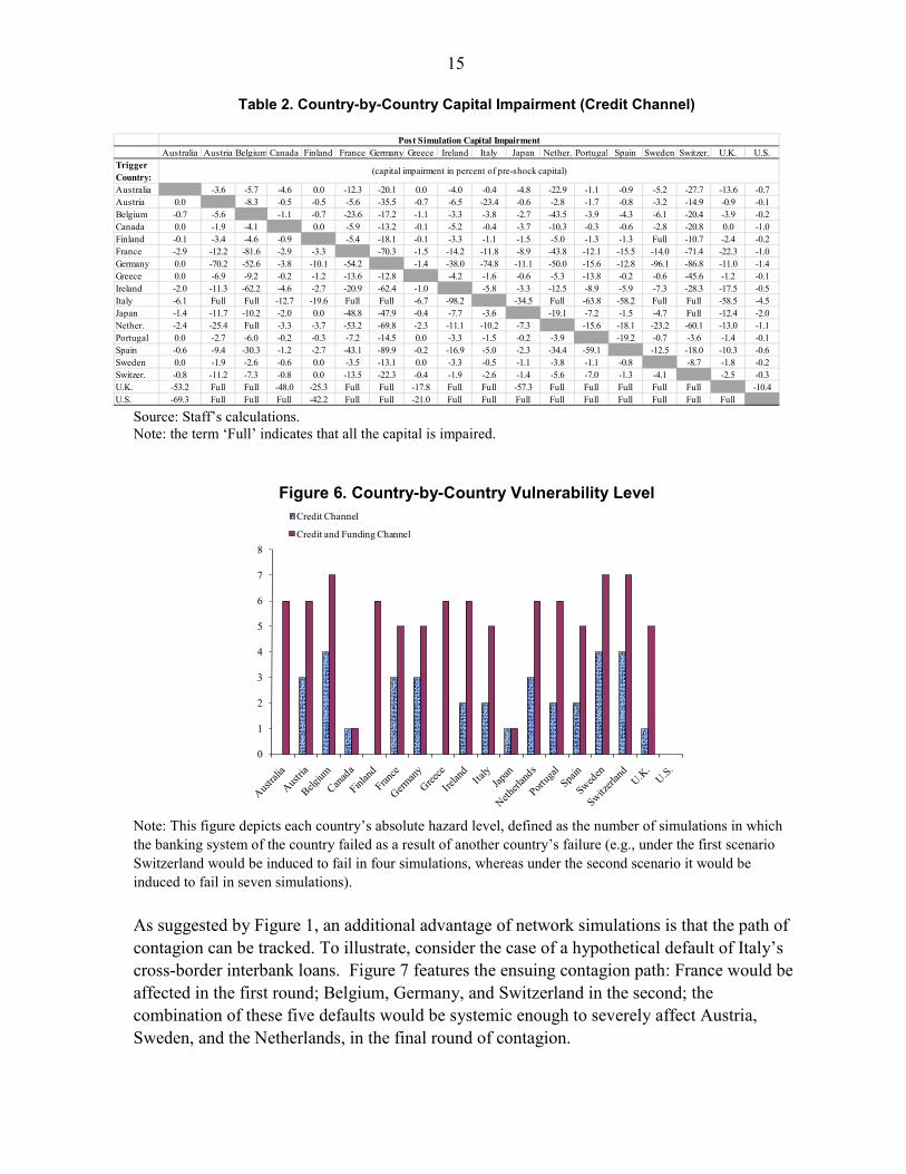
Table 4. Country-by-Country Capital Impairment (Credit and Funding Channel)

Australia Austria Belgium Canada Finland France Germany Greece Ireland Italy Japan Nether. Portugal Spain Sweden Switzer. U.K. U.S.Trigger Country:Australia -3.6 -6.0 -4.6 -0.1 -12.7 -20.1 -0.1 -4.8 -0.4 -4.8 -23.3 -1.1 -1.0 -5.3 -28.1 -16.5 -1.1Austria -0.5 -9.4 -0.6 -1.5 -6.2 -41.6 -3.6 -8.0 -25.2 -0.7 -4.4 -3.4 -1.5 -4.0 -16.9 -1.6 -0.4Belgium -1.9 -10.8 -1.8 -3.2 -30.6 -25.4 -8.2 -18.7 -7.5 -2.8 -66.4 -10.9 -8.4 -8.0 -22.7 -9.8 -2.0Canada -2.2 -2.5 -4.9 -0.7 -6.5 -14.5 -0.4 -7.6 -0.6 -3.8 -11.0 -0.6 -1.0 -3.8 -21.3 -2.7 -5.5Finland -0.6 -4.5 -5.7 -1.1 -6.0 -25.7 -0.6 -4.4 -1.4 -1.5 -6.3 -1.8 -2.2 Full -11.3 -3.8 -0.8France Full Full Full -72.4 Full Full Full Full Full -83.7 Full Full Full Full Full Full -72.1Germany Full Full Full -72.4 Full Full Full Full Full -83.7 Full Full Full Full Full Full -72.1Greece 0.0 -7.0 -9.4 -0.2 -1.2 -13.6 -12.9 -4.3 -1.6 -0.6 -5.3 -13.8 -0.2 -0.6 -45.7 -1.4 -0.1Ireland -3.3 -17.1 -63.9 -5.8 -2.7 -22.7 -70.7 -5.6 -9.3 -3.6 -14.1 -14.3 -9.2 -10.7 -29.2 -24.9 -1.4Italy Full Full Full -72.4 Full Full Full Full Full -83.7 Full Full Full Full Full Full -72.1Japan -16.7 -25.3 -25.8 -10.7 -7.1 -61.9 -76.8 -42.9 -22.0 -10.7 -30.5 -14.1 -6.7 -18.3 Full -33.1 -26.2Nether. -16.2 -35.0 Full -8.1 -9.9 -69.6 -97.3 -19.5 -34.2 -24.3 -8.8 -33.6 -33.7 -32.0 -66.8 -29.6 -7.9Portugal -0.1 -3.1 -6.5 -0.2 -0.4 -7.5 -15.3 -3.3 -4.0 -1.9 -0.3 -4.4 -21.6 -0.9 -4.3 -1.6 -0.1Spain Full Full Full -72.4 Full Full Full Full Full Full -83.7 Full Full Full Full Full -72.1Sweden -0.6 -2.9 -3.6 -0.8 -83.2 -4.1 -20.2 -0.3 -4.2 -0.8 -1.1 -4.9 -1.4 -1.6 -9.3 -3.2 -0.7Switzer. -7.5 -21.5 -15.2 -4.5 -2.7 -20.2 -37.2 -39.3 -9.6 -6.2 -7.8 -11.8 -11.6 -4.0 -11.2 -17.4 -16.4U.K. Full Full Full -72.4 Full Full Full Full Full Full -83.7 Full Full Full Full Full -72.1U.S. Full Full Full Full Full Full Full Full Full Full Full Full Full Full Full Full Full

Post Simulation Capital Impairment

(capital impairment in percent of pre-shock capital)

Source: Staff’s calculations. Note: the term ‘Full’ indicates that all the capital is impaired.

C. Simulations 3 and 4: Transmission of Shocks in the Presence of Risk Transfers

We now present two simulations that take into account the presence of risk transfers among the banking systems of the network. The results of these two simulations are presented in Figures 8 to 11, along with results from the previous simulations for ease of comparison. The point we want to make with these simulations is that the inclusion of risk transfers could change (sometimes even dramatically) the risk profile of the network. In particular, for the first distribution of risk transfer that we consider, the presence of risk transfers improves the resiliency of some countries to certain shocks (e.g., Belgium, the Netherlands, Sweden, and Switzerland) (Figure 9).15

15 Recall that the first distribution we assume is such that the distribution of risk transfers across referenced entities is the same as the distribution of direct credit exposures.

19

Figure 8. Number of Induced Failures—Uniform Distribution

0

2

4

6

8

10

12

14

16

18

Finland France Germany Italy Japan Netherlands Spain United Kingdom United States

Credit ChannelCredit (with Risk Transfer)Credit and Funding ChannelCredit and Funding Channel (with Risk Transfer)

Note: the figure shows the number of countries whose banking systems would fail, as of December 2007, as a result of the initial failure of each country.

Figure 9. Country-by-Country Vulnerability Level—Uniform Distribution

0

1

2

3

4

5

6

7

8 Credit ChannelCredit (with Risk Transfer)Credit and Funding ChannelCredit and Funding Channel (with Risk Transfer)

Note: This figure depicts each country’s absolute hazard level defined as the number of simulations in which the banking system of the country failed as a result of another country’s failure. Given that we do not know the true distribution of risk transfers across referenced entities, and to illustrate that it is key to know this distribution, we assumed an alternative distribution with a strong concentration of transfers on specific countries. In particular, we assumed that Belgium and Switzerland have only acquired risk transfers that have France as the referenced entity, and that the Netherlands has only acquired risk transfers that have Germany as the referenced entity. In other words, all the risk transfers that Belgium and Switzerland receive from all other countries are assumed to be referenced on France, and all the risk transfers that the Netherlands receives from all other countries are assumed to be referenced on Germany.

20

Figure 10: Number of Induced Failures—Biased Distribution

0

2

4

6

8

10

12

14

16

18

Finland France Germany Italy Japan Netherlands Spain United Kingdom

United States

Credit ChannelCredit (with Risk Transfer)Credit and Funding ChannelCredit and Funding Channel (with Risk Transfer)

Figure 11. Country-by-Country Vulnerability Level—Biased Distribution

0

1

2

3

4

5

6

7

8Credit ChannelCredit (with Risk Transfer)Credit and Funding ChannelCredit and Funding Channel (with Risk Transfer)

The results from assuming this distribution of risk transfers are presented in Figures 10 and 11, and show some differences from before. In particular, notice how, under the credit shock scenario, the inclusion of risk transfers increases the level of the systemic importance of France—now inducing 11 failures compared to none before. Similarly, Spain increases its systemic relevance under the credit-plus-funding shock—inducing now 14 failures compared to only one before. In terms of vulnerability levels (Figure 11), the results also point to an increased level of risk for almost all countries. In sum, these examples indicate that having accurate information on risk transfers across their three relevant dimensions (i.e., the originator of the risk transfers, the recipient, and the referenced party or entity) is key to the assessment of financial stability, as different distributions can give rise to very different risk profiles, as shown by the difference between Figures 8–9 and 10–11. Thus, having data that includes risks transfers enhances the knowledge of the risks actually present in a network—risks that could be realized if a distress

21

event were to occur. In other words, we view the variation in results—which in turn depends on the assumed distribution of risk transfers—as a call to improve on the collection and analysis of data on risk transfers.

IV. CONCLUDING REMARKS

Our illustration of network analysis has highlighted its usefulness as a cross-border surveillance tool. We have also stressed the need to give consideration to off-balance sheet risks in network analysis and proposed a simulation algorithm for this purpose. In addition, we emphasized the need for on- and off-balance sheet interbank linkages and cross-institutional linkages to be made increasingly available to those overseeing systemic stability. Going forward, financial regulators should continue to develop ways to systematically collect and analyze these data. Moreover, the global dimension of the 2007–09 crisis underscored the need to assess these exposures from a cross-border perspective, which would require further coordination and data sharing by national regulators. The analysis of how shocks reverberate throughout the system is important to get a sense of how a crisis could unravel once the initial shocks have taken place, assuming the authorities fail, or are too slow, to respond. This is not to say that the analysis of interconnectedness will unequivocally reveal where the next crisis will arise, but including an analysis of interlinkages in the supervisors’ repertoire may help identify institutions that need further scrutiny in terms of their vulnerability and/or level of systemic risk. If enough data are collected from various types of institutions, the perimeter of spillovers can be discerned and this could help distinguish which types of firms should be under a regulatory net. The 2007–09 crisis has proven that interconnectedness across institutions is present not only within the banking sector, but as importantly, with the nonbank financial sector (such as investment banking, hedge funds, etc.). In particular, the liquidity problems have demonstrated that roll-over risk can spill over to the whole financial system, thus requiring a better understanding and monitoring of both direct and indirect linkages. This paper also provides a potential approach to consider how to maintain an effective perimeter of prudential regulation without unduly stifling innovation and efficiency. It illustrates how network models should allow regulators to see which institutions are affected in subsequent rounds of spillovers and thus determine relative levels of supervision. Such an assessment would have to be conducted at regular intervals, as the structure of the network is likely to change over time. Similarly, network models can assist policymakers with their tough choices, such as how to design capital surcharges to lessen the too-connected-to fail problem. In sum, monitoring global systemic linkages will undoubtedly become increasingly relevant for financial regulators as well as for the IMF. Such monitoring can be enhanced in several ways:

22

• The development of reliable tools for this task should proceed expeditiously.

• Financial regulators need to strengthen their understanding of systemic linkages and improve their gathering of relevant data.

• New information-sharing agreements on cross-border financial exposures (including regulated and unregulated products and institutions) could strengthen the capacity of Fund members to provide it with the relevant data. In principle, such agreements could operate on a multilateral or bilateral basis and would ideally address both the domestic and cross-border dimensions.

23

REFERENCES

Allen, Franklin and Ana Babus, and others, 2007, Networks in Finance: Network-based Strategies and Competencies, Chapter 21, Working Paper 08–07 (Wharton School Publishing).

Allen, Franklin and Douglas Gale, 2000, Financial Contagion, Journal of Political Economy, Vol. 108, pp. 1–33.

Bank for International Settlements, 2008, Guidelines to the international consolidated banking statistics, (Basel: Bank for International Settlements).

Boss, Michael, Helmut Elsinger, Martin Summer and Stefan Thurner, 2005, “Network Topology of the Interbank Market,” Quantitative Finance, Vol. 4, pp. 677–684 (Austria: Department of Finance-Complex Systems Research Group).

Chan-Lau, Jorge, Marco Espinosa, Kay Giesecke, and Juan Solé, “Assessing the Systemic Implications of Financial Linkages,” Chapter 2, Global Financial Stability Report, April 2009.

Cifuentes, R., G. Ferrucci, and H. Shin, 2005, “Liquidity Risk and Contagion,” Journal of the European Economic Association, Vol. 3(2–3), pp. 556–66.

Degryse, Hans and Grégory Nguyen, 2007, “Interbank Exposures: An Empirical Examination of Contagion Risk in the Belgian Banking System,” International Journal of Central Banking, Vol., 3 No. 2.

Elsinger, Helmut, Alfred Lehar, and Martin Summer, 2006, “Risk Assessment for Banking Systems,” Management Science, Vol. 52, No. 9, pp. 1301–14.

Furfine, Craig H., 2003, “Interbank Exposures: Quantifying the Risk of Contagion,” Journal of Money, Credit and Banking, Vol. 35, No. 1.

Haldane, Andrew, 2009, “Why Banks Failed The Stress Test,” Marcus-Evans Conference on Stress-Testing, (London: Bank of England).

Hartmann, Philipp, Stefan Straetmans, and Casper G. de Vries, 2001, “Asset Market Linkages in Crisis Periods,” CEPR Discussion Paper No. 2916 (London: Centre for Economic Policy Research).

Hattori, Masazumi and Yuko Suda, 2001, “Developments in a Cross-Border Bank Exposure Network,” BIS International Financial Statistics, CGFS Workshop, “Research on Global Financial Stability,” BIS Workshop.

24

Issing, Otmar and Jan Krahnen, 2009, “Why the regulators must have a global ‘risk map,’” Financial Times of February 20, 2009.

Lagunoff, Roger and Stacey L. Schreft (2001), “A Model of Financial Fragility,” Journal of Economic Theory, Vol. 99, pp 220–264.

Márquez-Diez-Canedo, Javier and Serafín Martínez-Jaramillo, 2007, “Systemic Risk: Stress Testing the Banking System,” The International Conference on Computing in Economics and Finance.

Márquez-Diez-Canedo, Javier and Serafín Martínez-Jaramillo, 2009, “Systemic Risk: Stress Testing the Banking System”, International Journal of Intelligent Systems in Accounting, Finance and Management, Vol. 16:1, 2009.

McGuire, Patrick and Nikola Tarashev, 2008, “Global Monitoring with the BIS International Banking Statistics,” BIS Working Paper. No. 244, (Basel: Bank for International Settlements).

McGuire, Patrick and Götz von Peter, 2009, “The U.S. dollar shortage in global banking and the international policy response,” BIS Working Paper. No. 291, (Basel: Bank for International Settlements).

McGuire, Patrick and Philip Wooldridge, 2005, “The BIS consolidated banking statistics: structure, uses and recent enhancements,” BIS Quarterly Review, September, (Basel: Bank for International Settlements).

Memmel, Christoph and Ingrid Stein, 2008, “Contagion in the German Interbank Market,” (Frankfurt: Deutsche Bundesbank).

Müller, Jeanette, 2006, “Interbank Credit Lines as a Channel of Contagion” Journal of Financial Services Research 29:1 37–60, 2006 (Swiss National Bank).

Nier, Erlend, Jing Yang, Tanju Yorulmazer and Amadeo Alentorn, 2007, “Network Models and Financial Stability,” Journal of Economics Dynamics & Control, 31, pp. 2033–60.

Perotti, Enrico and Javier Suarez, 2009, “Liquidity insurance for systemic crises”, CEPR Policy Insight No. 31.

Stern, Gary H. and Ron J. Feldman, Too Big to Fail: The Hazards of Bank Bailouts

Stern, Gary H., 2008, “Repercussions From The Financial Shock,” (Minneapolis: Federal Reserve Bank).

(Washington, D.C.: Brookings Institution Press, 2004).

25

Upper, Christian, 2007, “Using Counterfactual Simulations to Assess the Danger of Contagion in Interbank Markets,” BIS Working Paper No. 234, (Basel: Bank for International Settlements).

Upper, Christian and Andreas Worms, 2004, “Estimating Bilateral Exposures in the German Interbank Market: Is There a Danger of Contagion?),” European Economic Review, 48 (2004), pp. 827–849.

Vassalou, Maria, and Yuhang Xing, 2004, “Default Risk in Equity Returns,” Journal of Finance, Vol. 59, pp. 831–68.

Vries, Casper G. de, 2005, “The Simple Economics of Bank Fragility,” Journal of Banking and Finance, Vol. 29(4), April, pp. 803–825.

Wells, Simon, 2002, “U.K. Interbank Exposures: Systemic Risk Implications,” Financial Stability Review, (London: Bank of England).

26

APPENDIX I: COMPARING RESULTS BASED ON THE IBB AND THE URB DATASETS

This appendix briefly summarizes the results from the simulations using ultimate risk basis data. As mentioned in Section II.C, URB data are consolidated by residency of the ultimate obligor (i.e., the party that is ultimately responsible for the obligation in case the immediate borrower defaults) and includes net risk transfers. Therefore, the simulation results could potentially differ substantially from those using immediate borrower basis data.

In order to assess whether the use of IBB or URB data would substantially alter our policy conclusions, we ran simulations using URB data. As Table A.1 below shows, the results of the simulations for the credit and the credit plus funding shocks retain some of their qualitative implications compared to our previous results: in both instances, the United Kingdom and the United States continue to be the two most systemic banking systems, and some other countries continue to maintain their (lower) profile as sources of contagion (e.g., Finland and Netherlands).

However, the comparison of IBB and URB data reveals some important differences for some other countries. For instance, Italy becomes less systemic with URB data in regard to credit shocks, going from seven to zero induced failures. Similarly, Germany, Italy, and Spain dramatically reduce their role under the credit plus funding shock scenario.

Table A.1: Comparing Simulation Results Using IBB and URB Datasets

CountryFailed Capital

(% of total capital)

Induced Failures

Contagion Rounds

Absolute Hazard 1/ Hazard Rate 2/ CountryFailed Capital

(% of total capital)

Induced Failures

Contagion Rounds

Absolute Hazard 1/ Hazard Rate 2/

Australia 2.6 -- -- -- 0.0 Australia 2.6 -- -- -- 0.0Austria 0.9 -- -- 3 17.6 Austria 0.9 -- -- 2 11.8Belgium 1.6 -- -- 4 23.5 Belgium 1.6 -- -- 3 17.6Canada 3.5 -- -- 1 5.9 Canada 3.5 -- -- -- 0.0Finland 1.2 1 1 -- 0.0 Finland 1.2 1 1 -- 0.0France 6.6 -- -- 3 17.6 France 6.6 -- -- 2 11.8Germany 3.6 -- -- 3 17.6 Germany 3.6 -- -- 2 11.8Greece 0.7 -- -- -- 0.0 Greece 0.7 -- -- -- 0.0Ireland 2.3 -- -- 2 11.8 Ireland 2.3 -- -- 2 11.8Italy 24.6 7 3 2 11.8 Italy 5.2 -- -- -- 0.0Japan 15.0 1 1 1 5.9 Japan 13.2 -- -- -- 0.0Netherlands 5.6 1 1 3 17.6 Netherlands 5.6 1 1 2 11.8Portugal 0.5 -- -- 2 11.8 Portugal 0.5 -- -- -- 0.0Spain 4.2 -- -- 2 11.8 Spain 4.2 -- -- 2 11.8Sweden 0.8 -- -- 4 23.5 Sweden 0.8 -- -- 3 17.6Switzerland 1.8 -- -- 4 23.5 Switzerland 1.8 -- -- 2 11.8United Kingdom 45.0 11 3 1 5.9 United Kingdom 39.3 9 3 1 5.9United States 96.2 14 3 -- 0.0 United States 73.8 10 4 -- 0.0

1/ Number of simulations in which that particular country fails. 1/ Number of simulations in which that particular country fails.2/ Percentage of failures as a percent of the number of simulations conducted. 2/ Percentage of failures as a percent of the number of simulations conducted.

Simulations with Immediate Borrower Basis Data Simulations with Ultimate Risk Basis DataEffects of Credit Shocks

27

CountryFailed Capital

(% of total capital)

Induced Failures

Contagion Rounds

Absolute Hazard 1/ Hazard Rate 2/ CountryFailed Capital

(% of total capital)

Induced Failures

Contagion Rounds

Absolute Hazard 1/ Hazard Rate 2/

Australia 2.6 -- -- 6 35.3 Australia 2.6 -- -- -- 0.0Austria 0.9 -- -- 6 35.3 Austria 0.9 -- -- 3 17.6Belgium 1.6 -- -- 7 41.2 Belgium 1.6 -- -- 4 23.5Canada 3.5 -- -- 1 5.9 Canada 3.5 -- -- 1 5.9Finland 1.2 1 1 6 35.3 Finland 1.2 1 1 3 17.6France 48.8 14 4 5 29.4 France 46.2 13 6 2 11.8Germany 48.8 14 5 5 29.4 Germany 4.4 1 1 3 17.6Greece 0.7 -- -- 6 35.3 Greece 0.7 -- -- 3 17.6Ireland 2.3 -- -- 6 35.3 Ireland 2.3 -- -- 3 17.6Italy 48.8 14 4 5 29.4 Italy 5.2 -- -- 3 17.6Japan 15.0 1 1 1 5.9 Japan 13.2 -- -- -- 0.0Netherlands 5.6 1 1 6 35.3 Netherlands 5.6 1 1 3 17.6Portugal 0.5 -- -- 6 35.3 Portugal 0.5 -- -- 3 17.6Spain 48.8 14 5 5 29.4 Spain 4.2 -- -- 3 17.6Sweden 0.8 -- -- 7 41.2 Sweden 0.8 -- -- 5 29.4Switzerland 1.8 -- -- 7 41.2 Switzerland 1.8 -- -- 3 17.6United Kingdom 48.8 14 3 5 29.4 United Kingdom 46.2 13 3 2 11.8United States 100.0 17 3 -- 0.0 United States 84.2 15 3 -- 0.0

1/ Number of simulations in which that particular country fails. 1/ Number of simulations in which that particular country fails.2/ Percentage of failures as a percent of the number of simulations conducted. 2/ Percentage of failures as a percent of the number of simulations conducted.

Effects of Credit and Funding ShocksSimulations with Immediate Borrower Basis Data Simulations with Ultimate Risk Basis Data