cover photos: spring chinook salmon, spring creek, … · tony grover. isab upper columbia tour of...
TRANSCRIPT


Cover design by Eric Schrepel
Cover photos: Spring Chinook salmon, Spring Creek, Methow River, Washington courtesy of
U.S. Fish and Wildlife Service. Wanapum Dam Juvenile Fish Bypass and California sea lion by
Tony Grover. ISAB Upper Columbia tour of Dillwater instream wood project site, Entiat River,
Washington by Erik Merrill.

Independent Scientific Advisory Board for the Northwest Power and Conservation Council,
Columbia River Basin Indian Tribes, and National Marine Fisheries Service
851 SW 6th Avenue, Suite 1100 Portland, Oregon 97204
Kurt D. Fausch, Ph.D., (ISAB Vice-chair) Professor Emeritus of Fisheries and Aquatic Sciences,
Department of Fish, Wildlife, and Conservation Biology at Colorado State University, Fort Collins, Colorado
Stanley Gregory, Ph.D., Professor Emeritus of Fisheries at Oregon State University, Corvallis, Oregon
William Jaeger, Ph.D., Professor of Applied Economics at Oregon State University, Corvallis, Oregon (also serves on IEAB)
Cynthia Jones, Ph.D., Eminent Scholar and Professor of Ocean, Earth, and Atmospheric Sciences; Director of the Center for Quantitative Fisheries Ecology; and A.D. and Annye L. Morgan Professor of Sciences at Old Dominion University, Virginia
Alec G. Maule, Ph.D., (ISAB Chair) Fisheries Consultant and former head of the Ecology and Environmental Physiology Section, United States Geological Survey, Columbia River Research Laboratory
Peter Moyle, Ph.D., Distinguished Professor Emeritus at the Department of Wildlife, Fish and Conservation Biology and associate director of the Center for Watershed Sciences, University of California, Davis
Katherine W. Myers, Ph.D., Research Scientist (Retired), Aquatic and Fishery Sciences, University of Washington, Seattle, Washington
Laurel Saito, Ph.D., P.E., Nevada Water Program Director, The Nature Conservancy of Nevada, Reno
Steve Schroder, Ph.D., Fisheries Consultant and Fisheries Research Scientist (Retired), Washington Department of Fish and Wildlife, Olympia, Washington
Carl J. Schwarz, Ph.D., Professor of Statistics and Actuarial Science at Simon Fraser University, Burnaby, British Columbia, Canada
Thomas Turner, Ph.D., Professor of Biology and Associate Dean for Research at the University of New Mexico, Albuquerque, New Mexico
ISAB Ex Officios and Manager
Michael Ford, Ph.D., Director of the Conservation Biology Program at the Northwest Fisheries Science Center, Seattle, Washington
Nancy Leonard, Ph.D., Manager, Fish, Wildlife, and Ecosystem Monitoring and Evaluation, Northwest Power and Conservation Council, Portland, Oregon
Zach Penney, Ph.D., Fisheries Science Manager at the Columbia River Inter-Tribal Fish Commission, Portland, Oregon
Erik Merrill, J.D., Manager, Independent Scientific Review, Northwest Power and Conservation Council, Portland, Oregon

i
ISAB Review of Spring Chinook Salmon in the Upper Columbia River
Contents List of Figures .................................................................................................................................. iv
List of Tables .................................................................................................................................. vii
Acknowledgments........................................................................................................................... ix
Executive Summary ......................................................................................................................... 1
1. Introduction .............................................................................................................................. 14
1.1. Review Charge .................................................................................................................... 14
1.2. Introduction to Upper Columbia Spring Chinook Salmon and Their Recovery ................. 16
1.3. Perspectives of Recovery ................................................................................................... 25
2. Review Process .......................................................................................................................... 27
3. Assessment of Upper Columbia River Spring Chinook ............................................................. 29
3.1. Identification of Limiting Factors ....................................................................................... 29
3.1.1. Potential Limiting Factors and Threats in UCR Tributary Basins ................................. 30
3.1.2. Consideration of Density Dependence in Analysis of Limiting Factors ....................... 38
3.1.3. Use of Life-Cycle Models to Identify Limiting Factors ................................................. 39
3.1.4. Influence of Factors Other Than UCR Habitat ............................................................. 43
3.1.5. Limiting Factors Conclusions ....................................................................................... 51
3.2. Comparison of UCR Spring Chinook Recovery with Snake River Spring Chinook Recovery
................................................................................................................................................... 53
3.2.2. Geography ................................................................................................................... 53
3.2.3. Conclusion for Snake River and Upper Columbia Chinook Comparison ..................... 75
3.3. Comparing the Abundance, Migration Timing, and Life History Strategies of Upper
Columbia River Summer and Spring Chinook ........................................................................... 76
3.3.1. Comparisons between Adult Summer and Spring Chinook Salmon ........................... 77
3.3.2. Comparisons between Juvenile Summer and Spring Chinook Salmon ....................... 87
3.4. Pinniped Predation ............................................................................................................. 95

ii
3.4.1. Background Information .............................................................................................. 95
3.4.2. ISAB’s Past Findings, Conclusions, and Recommendations......................................... 96
3.4.3. Conclusions about Pinniped Predation ..................................................................... 100
3.5. Recommendations ........................................................................................................... 103
4. Prioritization and Effectiveness of Habitat Restoration and Enhancement ........................... 107
4.1. Are Recovery Actions Being Prioritized and Sequenced Strategically? ........................... 108
4.1.1. Components for Effective Prioritization of Recovery Actions ................................... 109
4.1.2. Cost-effectiveness Estimates that Account for Time ................................................ 112
4.2. Evidence of Physical and Biological Responses to Past Habitat Restoration Projects ..... 114
4.2.1. Approaches for Measuring Effects of Habitat Restoration ....................................... 114
4.2.2. Evidence of Fish Responses to Habitat Restoration of Key Limiting Factors ............ 122
4.2.3. Application of Life-Cycle Models to Integrate Habitat Restoration with Other Effects
............................................................................................................................................. 128
4.2.4. Sample Designs and Sample Sizes Needed to Detect Biologically Significant Effects
............................................................................................................................................. 129
4.3. Approaches for Prioritizing Habitat Projects .................................................................... 130
4.3.1. Ecosystem Diagnosis and Treatment (EDT) Model ................................................... 130
4.3.2. Habitat Suitability Indices (HSI) ................................................................................. 133
4.3.3. Regional Technical Team (RTT) Biological Strategy ................................................... 135
4.4. Coordination and Interactions with Other Hs .................................................................. 137
4.4.1. Operational Structure ................................................................................................ 138
4.4.2. Strategies ................................................................................................................... 138
4.4.3. Coordinating Actions ................................................................................................. 139
4.5. Recommendations ........................................................................................................... 140
5. Research, Monitoring, Evaluation, and Validation ................................................................. 144
5.1. Research, Monitoring, and Evaluation (RME) Programs.................................................. 144
5.1.1. RME for Hatchery Programs in the Upper Columbia River ....................................... 144
5.2. Collecting Suitable Data, Testing and Validating Hypotheses ......................................... 147
5.3. Changes in the RME Process ............................................................................................ 151
5.4. Uncertainties Associated with Hatchery Fish Interactions in the Upper Columbia......... 155
5.4.1. Sufficiency of the Current M&E Program .................................................................. 155

iii
5.4.2. Effect of Historical and Current Hatchery Programs on Fitness of the Upper Columbia
Spring Chinook ESU.............................................................................................................. 155
5.4.3. Recommendations ..................................................................................................... 166
6. Modeling ................................................................................................................................. 173
6.1. Specific Comments about Life Cycle Models ................................................................... 173
6.1.1. Food Web Model for the Methow River ................................................................... 177
6.1.2. Wenatchee Model ..................................................................................................... 178
6.1.3. ISEMP Model for the Entiat River .............................................................................. 179
6.1.4. Ecosystem Diagnosis and Treatment (EDT) Model ................................................... 180
6.1.5. Recommendations ..................................................................................................... 180
7. Appendices .............................................................................................................................. 182
Appendix A. List of Presentations to ISAB ............................................................................... 182
Appendix B. Comparison of Ocean and Estuary Life Histories................................................ 185
Appendix C. Review of Appendix C in Murdoch et al. (2011) ................................................. 190
Appendix D. Editorial Comments on Murdoch et al. (2011). .................................................. 197
Appendix E. Review of BACI Analysis ...................................................................................... 201
Appendix F. Review of Hillman et al. 2017 ............................................................................. 211
Appendix G. Null Hypothesis Significance Testing (NHST) ...................................................... 228
8. Literature Cited ....................................................................................................................... 230

iv
List of Figures Figure 1.1. Map of mainstem Columbia River and location of the Wenatchee, Entiat, and
Methow basins .............................................................................................................................. 17
Figure 1.2. Map of spring Chinook salmon distributions in the Wenatchee River basin ............. 18
Figure 1.3. Map of spring Chinook salmon distributions in the Entiat River basin ...................... 19
Figure 1.4. Map of spring Chinook salmon distributions in the Methow River basin .................. 20
Figure 1.5. Abundance of natural origin spring Chinook salmon in the Upper Columbia River
from 1960-2016 ............................................................................................................................ 23
Figure 3.1. Estimates of relative contribution to habitat impairment as a limiting factor for the
Upper Columbia River spring Chinook salmon ............................................................................. 33
Figure 3.2. Cumulative number of habitat projects implemented in the Upper Columbia region
between 1996-2012 by project type ............................................................................................ 35
Figure 3.3. Assessment of the quantity (miles, acres, numbers) of recovery actions in the UCR
between 1996-2012 by year (red) and cumulatively (blue) ......................................................... 35
Figure 3.4. Number of limiting factors identified for all fish species of concern in the
Wenatchee, Entiat, and Methow Subbasin Plans ......................................................................... 37
Figure 3.5. Evidence for density dependence in Upper Columbia River spring and summer
Chinook populations, brood years 1980 to ~2005 ....................................................................... 39
Figure 3.6. Diagram of the life-cycle model for spring Chinook salmon in the Wenatchee
subbasin. ....................................................................................................................................... 40
Figure 3.7. Population responses to cumulative effects of scenarios of management actions,
measured by median spawner abundance and by estimates of extinction risk .......................... 41
Figure 3.8. Percent change in annual spawners relative to current conditions for scenarios of
historical conditions, restoration actions, no restoration, and increased habitat degradation in
the Wenatchee Basin .................................................................................................................... 42
Figure 3.9. Actual (open circles) and predicted (filled circles) mean Fish Travel Time (FTT, days)
for yearling Chinook between RIS -> MCN and MCN -> BON (upper graph) and relative variable
importance for predictive model of FTT from six covariates (lower graph) ................................ 47
Figure 3.10. Actual (open circles) and predicted (filled circles) for Instantaneous Mortality for
yearling Chinook between RIS -> MCN and MCN -> BON (upper graph of pair) and variable
importance (lower graph of pair) ................................................................................................. 48

v
Figure 3.11. Actual (open circles) and predicted (filled circles) of in-river survival for yearling
Chinook between RIS -> MCN and MCN -> BON .......................................................................... 48
Figure 3.12. SARs (including jacks) for MCN-BON (upper graph) and RRE-BON (lower graph) for
Upper Columbia spring Chinook with confidence intervals computed using bootstrapping ...... 49
Figure 3.13. Spring out-migrants’ yearling spring Chinook juvenile survival from RIS to MCN (top
graph) ............................................................................................................................................ 50
Figure 3.14. Mean spawning elevation available to spring Chinook salmon in the Upper
Columbia River and spring/summer Chinook in the Snake River ................................................. 57
Figure 3.15. Mean annual precipitation in the Upper Columbia and Snake river spring Chinook
ESU subbasins ............................................................................................................................... 57
Figure 3.16. Hydrologic regime of Upper Columbia spring Chinook and Snake River
spring/summer Chinook ESUs ....................................................................................................... 58
Figure 3.17. Geomorphic condition based on CHaMP analyses of subbasins of ESUs in the Upper
Columbia River (three on the right) and representative subbasins in the Snake River (three on
the left).......................................................................................................................................... 58
Figure 3.18. Abundance and productivity gaps for Snake River Spring/Summer Chinook ESU
populations ................................................................................................................................... 61
Figure 3.19. Estimates of in-river survival probability for release cohorts of hatchery (H) and
wild (W) yearling Chinook salmon (CH1) migrating in the LGR–MCN and RIS–MCN reaches,
1998–2016 .................................................................................................................................... 63
Figure 3.20. Snake River spring/summer Chinook salmon aggregate smolt to adult return rates
(solid blue), Upper Columbia spring Chinook (blue dashed line) ................................................. 66
Figure 3.21. Exploitation rate (total harvest) for Upper Columbia River spring Chinook salmon 68
Figure 3.22. Average mean passage date (points) at Bonneville Dam for wild spring and summer
Chinook salmon populations in 1998–2015 ................................................................................. 69
Figure 3.23. Number of ecological concerns (please see text for definition) for the three Upper
Columbia spring Chinook populations (yellow bars) and Snake River spring/summer Chinook
populations (all other bars) .......................................................................................................... 75
Figure 3.24. The abundance of natural origin adult summer (black circles) and spring Chinook
(open circles) returning to Upper Columbia River subbasins ....................................................... 77
Figure 3.25 A&B. Counts of hatchery and natural origin adult summer (black circles) and spring
Chinook (open circles) at Rock Island Dam from 1933 through 1968 (part A) and from 1973
through 2010 (part B) ................................................................................................................... 79
vi
Figure 3.26. The spatial distribution of spring and summer Chinook salmon redds in the Entiat
subbasin. ....................................................................................................................................... 86
Figure 3.27. Percentage of natural origin adults returning in the same year to the Wenatchee
and Methow subbasins that utilized the juvenile subyearling (A) and reservoir (B) strategies and
percentage of Wenatchee (black circles) and Methow (red circles) of naturally produced adults
that used the subyearling (C) and yearling (D) life histories by return year ................................ 95
Figure 3.28. Estimates of consumption of Chinook salmon by pinniped predators in the
Columbia River, with uncertainty, in terms of the biomass (primary axis) and number
(secondary axis) of Chinook salmon consumed, 1975-2015 ...................................................... 101
Figure 3.29. Preliminary estimated pinniped predation at Bonneville Dam in 2017, compared to
the 10-yr average (Tidwell et al. 2017) ....................................................................................... 101
Figure 3.30. The estimated number of upriver spring/summer Chinook mortalities (95%
confidence interval) in the Columbia River below Bonneville Dam ........................................... 102
Figure 4.1. Framework for assessing project management success .......................................... 110
Figure 4.2. Proportion of published studies of placing structures made of large wood that
reported positive effects, negative effects, or no change (equivocal) in physical habitat, fish
(juvenile and adult salmonids, or non-salmonids), or macroinvertebrate density or diversity
(Inverts) ....................................................................................................................................... 127
Figure E.1. Conceptual sources of variation in a BACI experiment with 1 supplemental stream (S)
and one reference stream (R) ..................................................................................................... 203
Figure E.2. Simulated results under three scenarios .................................................................. 204
Figure E.3. Simulated results under three scenarios with 1 supplemented stream and 3
reference streams ....................................................................................................................... 207
Figure E.4. Simulated results under three scenarios with 1 supplemented stream and 1
reference stream ........................................................................................................................ 209

vii
List of Tables Table 3.1. Rankings of ecological concerns across the four basins of the UCR ............................ 34
Table 3.2. Change in the number of smolts and spawners relative to current scenario from
improvement and degradation of individual habitat variables with other variables held at
estimated current values .............................................................................................................. 42
Table 3.3. Harvest rates for Chinook salmon in the Columbia River during the spring harvest
season ........................................................................................................................................... 51
Table 3.4. Intrinsic size and complexity ratings for historical populations within the Upper
Columbia River Spring Chinook ESU ............................................................................................. 55
Table 3.5. Intrinsic size and complexity ratings for extant Snake River Spring Chinook ESU
populations organized by Major Population Groupings ............................................................... 55
Table 3.6. Probability of smolt survival when migrating from hatcheries in the Upper Columbia
River (UCR) or the Snake River (SNR) to either Lower Granite Dam (LGR) or McNary Dam (MCN)
and from MCN to Bonneville Dam (BON) ..................................................................................... 64
Table 3.7. Reach-specific bird predation rates (percentage of tagged fish consumed, as means
with SE) and total mortality of tagged yearling Chinook salmon released into the mid/Upper
Columbia River .............................................................................................................................. 64
Table 3.8. Smolt-to-adult return rate for Upper Columbia River (UCR) natural origin spring
Chinook salmon (Sp Chin) and Snake River (SNR) natural origin spring/summer Chinook (Sp/Su
Chin) that passed Lower Granite Dam (LGR), Rocky Reach Dam (RRE) or McNary Dam (MCN) and
were subsequently detected at Bonneville Dam (BOA) as returning adults (jacks included) ...... 67
Table 3.9. Comparison of limiting factors for Upper Columbia River spring Chinook salmon
(UCRSC) with those for Snake River spring/summer Chinook salmon (SNRSC) ........................... 73
Table 3.10. Percentage of Upper Columbia River spring and summer Chinook passing over
Bonneville Dam by date ................................................................................................................ 81
Table 3.11. Return year and arrival timing relationships to the survival of adult Chinook salmon
in the lower Columbia River ......................................................................................................... 82
Table 3.13. Estimated pNOB, pHOS, and PNI values for Upper Columbia River Chinook salmon
populations ................................................................................................................................... 85
Table 3.14. Distribution patterns of summer and spring Chinook salmon juveniles rearing in the
Entiat subbasin during the summer (August) and winter (March) ............................................... 89
Table 3.15. Comparisons between assumed and observed life history patterns in Upper
Columbia River summer and spring Chinook juveniles ................................................................ 92

viii
Table 3.16. Smolt-to-adult return rates (SARs) in Chinook salmon returning to the Entiat that
adopted different life histories (yearling and subyearling) and juvenile rearing areas (natal
stream, reservoir, and ocean) by brood year ............................................................................... 93
Table 3.17. Results of Kendall’s Tau correlations conducted on the percentages of adults
possessing different juvenile life histories that returned in the same year but to different Upper
Columbia subbasins ...................................................................................................................... 94
Table 4.1. A hierarchy of approaches for measuring effects of habitat enhancement on
salmonids in streams and rivers ................................................................................................. 118
Table 5.1. The hatchery programs in the Upper Columbia River as of 2015 .............................. 146
Table 5.2. The objectives and management questions that were presented in the monitoring
and evaluation program of Murdoch et al. (2011) ..................................................................... 148
Table 5.3. Productivity and monitoring indicators along with objectives, and targets for Upper
Columbia River hatchery programs ............................................................................................ 153
Table 5.4. The number and spawning success of spring and summer Chinook transplanted into
the Wenatchee River from 1939-1943 ....................................................................................... 158
Table 5.5. Summary of some of the assessments made on NOR and HOR spring Chinook
originating from the Methow, Chewuch, and Twisp supplementation programs ..................... 163
Table 5.6 Average stray rates by brood year in spring Chinook salmon produced by Upper
Columbia River hatchery programs ............................................................................................ 165
Table 6.1. Summary of features of the life-cycle models developed for the Upper Columbia ESU
..................................................................................................................................................... 174
Table B.1. Comparison of smolt-to-adult (ocean and estuary) life history traits and status of
Upper Columbia (UC) spring Chinook and Snake River spring/summer Chinook ...................... 185
Table E.1. Mean abundance in two streams, before and after supplementation is started ..... 201

ix
Acknowledgments Numerous individuals and institutions assisted the ISAB with this report. Their help and
participation are gratefully acknowledged. Perhaps more than any past ISAB effort, this review
relied on the guidance and collaboration of scientists and restoration practitioners outside the
ISAB, Council, NOAA, and CRITFC.
A few individuals were especially helpful in providing input, support, information and
presentations from the assignment’s development to its completion: Greer Maier (Upper
Columbia Salmon Recovery Board [UCSRB]), Andrew Murdoch (Washington Department of Fish
and Wildlife [WDFW]), Tom Kahler (Douglas County Public Utility District [PUD]), Catherine
Willard (Chelan County PUD), Todd Pearsons (Grant County PUD), and Tracy Hillman (UCSRB
Regional Technical Team, BioAnalysts).
The following researchers and practitioners gave excellent presentations at site tours or
meetings:
Steve Parker and Brandon Rodgers (Yakama Nation)
John Arterburn (Confederated Tribes of the Colville Reservation)
Bill Gale, Tom Desgroseillier, Robes Parrish, and Greg Fraser (U.S. Fish and Wildlife Service [USFWS])
Jeromy Jording, Michelle Wargo Rubb, Jeff Jorgensen, Mark Sorel, Chris Jordan, and Robby Fonner (NOAA Fisheries)
Steve Kolk (U.S. Bureau of Reclamation)
Sean Welch (Bonneville Power Administration)
Jeremy Cram, Charlie Snow, and Dan Rawding (WDFW)
Greg Mackey and Shane Bickford (Douglas PUD)
Lance Keller, Alene Underwood, and Ian Adams (Chelan PUD)
Curtis Dotson, Peter Graf, and Tom Dresser (Grant PUD)
Mike Kane and Jennifer Hadersberger (Chelan County Natural Resource Department [CCNRD])
Jason Sims and Mike Cushman (Cascadia Conservation District)
Mickey Fleming (Chelan-Douglas Land Trust)
John Crandall (Methow Salmon Recovery Foundation)
Aaron Penvose (Trout Unlimited)
Keith Van den Broek (Terraqua Inc., Entiat IMW)
Brandon Chasco (Oregon State University)
Phil Roni (Cramer Fish Sciences)
Other individuals were responsive to inquiries, helped develop the review, or added critical
information for the report, especially Denny Rohr (consultant), Melody Kreimes and Joy Juelson
(UCSRB), BJ Kieffer and Conor Giorgi (Spokane Tribe of Indians), Randall Friedlander and Casey
Baldwin (Colville Confederated Tribes), Kurt Truscott and Tracy Yount (Chelan PUD), Deane
x
Pavlik-Kunkel (Grant PUD), Dale Bambrick and Tim Beechie (NOAA Fisheries), Tom Iverson
(consultant for Yakama Nation), Karl Polivka (U.S. Forest Service), Sarah Walker (Terraqua, Inc.),
and Eric Doyle (ICF International).
Bin Quan (QW Consulting) was extremely helpful in creating maps and tracking down numbers
that are included in the report.
The ISAB Ex Officio members helped define our review, organized briefings, provided context,
and commented on drafts: Mike Ford, Zach Penney, and Nancy Leonard. Tom Skiles of CRITFC
assisted Zach Penney in his Ex Officio duties, helped organize a site tour, and provided useful
contextual information.
The Council, NOAA, and CRITFC administrative staff supported our numerous meetings and
briefings. Eric Schrepel (Council staff) improved the quality of the report’s formatting and
graphics, and Kendra Coles helped with citations.

1
Executive Summary In response to a request from the Independent Scientific Advisory Board’s (ISAB) Administrative
Oversight Panel (April 2017 memorandum), the ISAB reviewed habitat assessment, research
and monitoring, and prioritization and coordination of recovery actions for spring Chinook
salmon in the Wenatchee, Entiat, and Methow basins of the Upper Columbia River. The review
was requested because spring Chinook populations in the Upper Columbia River remain at high
risk of extinction despite a decade of habitat restoration actions guided by the 2007 Upper
Columbia Spring Chinook Salmon and Steelhead Recovery Plan.
The Upper Columbia Salmon Recovery Board, tribes, state and federal managers, public utility
districts (PUDs), and local groups assisted the ISAB in its review. Leaders in these groups
presented valuable information to aid our review, including a field review of the Wenatchee
and Entiat subbasins and more than 25 presentations. The recovery program in the Upper
Columbia Basin is one of the better examples of an explicit strategy to guide local recovery
actions, monitoring, and adaptive management.
The ISAB developed the following key findings and recommendations to address the Oversight
Panel’s four major questions (see section 1.1 of the Report for the specific questions):
1. Is the identification of limiting factors for Upper Columbia River spring Chinook based on sound scientific principles and methods?
The Upper Columbia Salmon Recovery Board (UCSRB) has refined its analysis of limiting factors
substantially since the first assessments in the late 1990s. The scientific principles for
identifying factors limiting the recovery of Upper Columbia spring Chinook salmon are generally
sound. Limiting factors are defined in the 2007 Upper Columbia Recovery Plan as
environmental conditions that negatively affect the abundance, productivity, spatial structure,
and diversity of salmon populations. Analysis of limiting factors based on current habitat
conditions is useful for prioritizing restoration actions. The UCSRB recently refined their
traditional habitat-based approaches by weighting limiting factors based on anticipated survival
benefits and geographic extent. Assessments of limiting factors are used to prioritize recovery
actions, and the recent history of restoration is relatively consistent with the rankings of
limiting factors.
Limiting factors analyses of the headwater basins do not incorporate the full life history of the
fish and their geographic range from egg to adult spawner. Limiting factors for spring Chinook
salmon in the Upper Columbia have been assessed through traditional freshwater habitat
assessments, analysis of density dependence, and life cycle models. Each have important
applications in management of the four Hs, but to date there has been no integration of all
three approaches.

2
Empirical density dependence data and life-cycle modeling conducted by regional scientists in
the Upper Columbia provide more holistic analyses of limiting factors over the full life cycle of
spring Chinook salmon than traditional assessments of habitat-related limiting factors in
freshwater. These traditional habitat-based approaches can be used in planning and prioritizing
restoration actions, but more explicit integration of these approaches would strengthen future
efforts.
The goal of the UCSRB program is to identify limiting factors within four categories of human
impacts (threats), including habitat, harvest, hydrosystem, and hatcheries (four Hs), both within
and outside the Upper Columbia watershed. While the Recovery Plan recognizes the influence
of all Hs, analysis of limiting factors has not integrated the four Hs to determine which have the
greatest influence on spring Chinook populations. Life-cycle models for these subbasins are
beginning to provide evidence that addresses all Hs, but they are in early stages of
development. Limiting factors are considered to be working hypotheses that can be tested, and
monitoring and adaptive management are critical for understanding and addressing them. Key
uncertainties such as ocean productivity and global climate change are identified.
Recommendation: The ISAB recommends integrating the results of the different
approaches—limiting factors analysis, density dependence analysis, life-cycle modeling—for
identifying limiting factors to guide future revision of the Biological Strategy of the UCSRB’s
Regional Technical Team and the Recovery Plan for spring Chinook salmon. This integration
will require a collaborative process that includes significant participation by experts,
practitioners, and management teams from all Hs.
1a. Are Snake River spring Chinook doing better than Upper Columbia spring Chinook, in terms of abundance, diversity, spatial structure, and productivity?
Differences in geography and biology result in differences in the spatial structure and diversity
of the two evolutionarily significant units (ESUs). Nonetheless, most measures of population-
level abundance and productivity for spring Chinook and assessments of habitat are similar in
the two ESUs. In-river survival of spring Chinook smolts migrating in the Upper Columbia as
compared to Snake River spring/summer Chinook smolts does not appear to differ. Smolt-to-
adult survival (SAR) of wild Upper Columbia and Snake River Chinook also does not appear to
differ.
Because the Snake River ESU has many more populations and larger absolute abundance than
the Upper Columbia ESU, the consequences of the differences in relative proportions may be
worse for Upper Columbia spring Chinook than for Snake River spring/summer Chinook. If in-
river survivals are equal for the two ESUs, adverse events create greater risks for the Upper

3
Columbia populations because they are less buffered by adjacent populations. For example, if
the proportion of losses to pinniped predation continues to increase but are the same for the
two ESUs, the reduction of Upper Columbia spring Chinook spawners, which have smaller
numbers, might reduce their ability to find mates on the spawning grounds. Thus, the ISAB
believes that the Upper Columbia spring Chinook ESU may be exposed to greater risks than the
Snake River spring/summer Chinook ESU. The same concern was expressed by NOAA Fisheries
when the Upper Columbia ESU was originally listed as endangered and the Snake River ESU as
threatened, listings that were not changed in the most recent reviews.
Recommendation: The ISAB recommends continued comparison of Chinook recovery in both
ESUs to determine which restoration actions are most effective. Rigorous RME programs are
essential to understand the trends and factors that influence them in these two basins.
1b. Differences between summer Chinook and spring Chinook in the Upper Columbia
Differences between spring and summer Chinook in the Upper Columbia could identify limiting
factors for spring Chinook. Summer Chinook have greater juvenile life history diversity than
spring Chinook and therefore may have greater intrinsic resilience to limiting factors than
spring Chinook. Summer Chinook enter the estuary as subyearlings and yearlings over a much
longer period than spring Chinook. Later out-migration timing of summer Chinook subyearlings
coincides with the increased spill regime that was established to reduce dam related
mortalities. Their outmigration timing is also better synchronized with increased flows and
higher turbidity due to spring run-off. Smaller size at emigration may reduce vulnerability of
summer Chinook to avian predators that prefer larger prey (e.g., Caspian terns). Summer
Chinook typically rear for shorter periods in tributaries than spring Chinook and are less likely to
experience capacity limitations or survival bottlenecks in subbasins. Contrary to previous
understanding, some Upper Columbia spring Chinook juveniles rear in mainstem reservoirs for
prolonged periods. The lower 235 river kilometers between Bonneville Dam and the ocean was
identified as a feeding area for juvenile salmonids where competition for resources with other
species and age classes may occur.
Recommendation: The ISAB recommends continued investigations of the effects of summer
Chinook on spring Chinook in Upper Columbia River subbasins, including effects of hatchery
practices, redd superimposition, competition, outmigration behavior, relative rates of
survival and behavior in the mainstem Columbia, and the relative effects of pinnipeds and
harvest in the lower river and estuary. Management actions should be developed to lessen
constraints on spring Chinook abundance as information becomes available.

4
Analysis of demographic trends in the Upper Columbia may reveal relationships between
summer and spring Chinook more effectively if adult returns are grouped by broodyear.
Juveniles are counted by cohort or year class, and adults should be counted on a similar basis.
1c. Are pinnipeds potentially a significant source of mortality for Upper Columbia spring Chinook? Can the effect of pinniped predation of Upper Columbia spring Chinook be quantified?
Pinnipeds are potentially a significant source of mortality for Upper Columbia spring Chinook
adults. However, population-specific estimates of predation impacts on Upper Columbia spring
Chinook were not available to the ISAB at the time of this review. The estimated consumption
of all Chinook salmon populations combined by pinnipeds in the Columbia River increased
sharply over the past decade, likely exceeding mortality by fisheries. Potential impacts varied by
pinniped species, salmon life stage, and run timing. In 2017, the reduced salmonid runs and
persistently high numbers of pinnipeds later in the migration period suggested the total impact
by pinnipeds on this year’s salmonid run may be large.
Efforts to quantify the effects of pinniped predation on Upper Columbia spring Chinook
continue to make progress. However, additional data and evaluation of uncertainties in the
estimates and model structure are needed to improve estimates of pinniped predation on
Upper Columbia spring Chinook salmon. In-river mortality of upriver spring/summer Chinook
salmon adults peaked in 2014 and 2015 (~100,000 fish) and decreased in 2016 and 2017 to
levels (~22,000 fish) similar to those in 2010-2013 (~31,000 fish). Estimates of adult Chinook
mortality are highest in the estuary and Bonneville tailrace. A recent modeling study reported
that additional sea lion predation on Columbia River Chinook salmon in the ocean (ocean age-1
salmon) may be similar to in-river consumption rates of adult Chinook.
Recommendation: The ISAB reiterates its recommendations from past reviews (see 3.4.2),
and recommends proceeding with the pinniped recommendations listed in NOAA Fisheries
2016 Five-Year Upper Columbia Status Report: “(1) expand pinniped monitoring efforts to
assess interactions between pinnipeds and listed species, (2) maintain predatory pinniped
management actions at Bonneville Dam to reduce the loss of upriver listed salmon and
steelhead stocks, (3) complete life-cycle/extinction risk modeling to quantify predation rates
by predatory pinnipeds on listed salmon and steelhead stocks in the Columbia River and
Willamette River, and (4) expand research efforts in the Columbia River estuary on survival
and run timing for adult salmonids migrating through the lower Columbia River to Bonneville
Dam.” The second recommendation is a necessary precautionary measure while better data
are collected.
In addition, the ISAB recommends identifying and investigating other potentially significant
sources of mortality of Upper Columbia spring Chinook smolts and adults in the Columbia

5
River plume/ocean shelf habitats, estuary, and lower mainstem and tributaries. New
information from NOAA’s tagging and modeling efforts revealed important data gaps,
including lack of population-specific survival estimates for Upper Columbia spring Chinook.
The ISAB recommends use of a variety of approaches to quantify pinniped predation impacts,
such as the ongoing tagging studies and coast-wide bioenergetics/life-cycle modeling.
Comparison of multiple models could reduce structural uncertainty (e.g., comparing a
bioenergetics approach to individual-based models or time series models).
2a. Are habitat recovery actions being prioritized and sequenced strategically? How should habitat projects be prioritized?
The ISAB found the UCSRB’s system for solicitation, review, and project design to be
scientifically sound with regard to habitat conditions and potential effects of hatcheries and the
hydrosystem. Current methods of prioritization (e.g., Ecosystem Diagnosis and Treatment (EDT)
Model, Habitat Suitability Index (HSI), and Regional Technical Team’s (RTT) Biological Strategy)
are useful for planning and prioritizing ecological concerns and related habitat restoration
actions.
The UCSRB focuses most attention on determining which kinds of actions will be biologically
beneficial toward recovery of Upper Columbia spring Chinook and assesses fish abundance,
productivity, and risk of extinction. The procedure for characterizing cost effectiveness is not
quantitative and does not provide a rigorous basis for prioritizing actions. If funds are unlimited,
there would be no need to prioritize actions, but that clearly is not the case. The criteria used
by the Regional Technical Team and the Citizens Advisory Committee are vague, and the results
are weighted so they have little influence on project priorities. Cost effectiveness is considered
by the UCSRB and the Salmon Recovery Board, but there is no explicit analysis and the
evaluations are not documented.
The existing prioritization process could be strengthened by incorporating explicit analysis of
performance, time, and cost in a cost-effectiveness assessment. Studies have shown that doing
so can improve outcomes by an order of magnitude. However, this will require empirical or
other ways of estimating biological benefits as well as estimating project costs. Effectiveness in
terms of smolts per adult (i.e., freshwater productivity) is difficult to estimate, as are the effects
over time, but developing a clear method would better highlight knowledge gaps. In the
interim, eliciting estimates from a set of experts could provide an objective starting point for
assessing relative cost effectiveness of projects. We recommend developing a standard
estimation of cost-effectiveness ratios for evaluating each proposed project and describe a
simplified approach as a starting point (section 4.1.2).

6
Recommendation: The ISAB recommends applying a transparent cost-effectiveness analysis
of each proposed project, perhaps by using the approach in the simple example we describe
in this Report’s Box 4.1 as a starting point. The lack of rigorous cost effectiveness analysis and
its minor influence on prioritization of restoration actions for all Hs limit the USCRB and
participants in their recovery efforts. This is a common deficiency throughout the Columbia
Basin, but such analyses would allow the program to use its limited resources more
effectively.
2b. Is there evidence that past projects have improved habitat for this ESU? What types of habitat projects should be prioritized in the future?
There is evidence that some types of projects have improved habitat more than others. The
ISAB found that there is sufficient evidence that protecting habitat, removing barriers to restore
connectivity, and reconnecting side channels and floodplains have positive effects on
anadromous salmonids, including spring Chinook salmon. Projects at different scales within the
Upper Columbia provide strong evidence that structures that increase pools and habitat
complexity can increase fish production, survival, and abundance. Effects of log and boulder
structures should be measured to understand effects of specific types of structures in particular
watersheds.
Empirical data and modeling from the Upper Columbia and other locations within and beyond
the Columbia River Basin support ranking habitat protection as a high priority, followed by
removing barriers, and reconnecting floodplains and side channels. Increasing habitat
complexity using log and boulder structures is a useful short-term approach, but a long-term
strategy is needed to restore processes that maintain channel complexity and supply and retain
large wood in rivers. Less information was available on projects that increase instream flows or
address water quality, although these can also be effective.
Recommendation: Projects that restore and sustain key fluvial and ecological processes
should be considered high priority, given predictions for future climate and building on the
successes of the projects completed so far. A key goal will be to provide habitats that are
resilient to changing conditions and extreme events, and ones that provide connected
habitats needed to sustain the full range of life history diversity among spring Chinook in the
Upper Columbia.
The ISAB recommends designing rigorous experiments and continued careful monitoring to
measure the effectiveness of habitat restoration practices in the upper Columbia subbasins
across a hierarchy of biological responses, including use of habitats by fish, and their

7
abundance, growth, survival, and productivity. Viable Salmonid Population (VSP)
measurements should be compared against model predictions to verify and improve
modeling approaches.
2c. How well are actions in other management sectors (all H’s, i.e., habitat and hydrosystem, hatcheries, and harvest) aligned with recovery efforts?
The UCSRB has developed a useful process for prioritizing restoration projects and coordinating
recovery actions. The regional recovery plan, limiting factors assessment, life-cycle models, and
monitoring provide critical information for recovery actions. However, a continued challenge is
coordinating groups in the three subbasins responsible for the four Hs. More than 16
independent coordinating committees and several other major working groups make critical
decisions on recovery actions. Currently, there is no process for integrating their separate
efforts into a coordinated action plan across the three subbasins.
Coordination of habitat actions and harvest management and hatchery operations also could
be improved. Continued management to reduce effects of hatcheries on fitness of spring
Chinook in the three subbasins need to be coordinated with prioritizing and implementing
habitat restoration projects to improve recovery efforts. Collaborative discussions of the UCSRB
and harvest co-managers about influences of adult return rates on spring Chinook recovery and
potential harvest recommendations would strengthen recovery efforts of the UCSRB.
Recommendation: The ISAB encourages the UCSRB and its participants to develop a
systematic, collective process for coordination of the actions, monitoring efforts, and
decisions across the numerous working groups and coordinating committees in the three
subbasins.
If return of adult spawners or recruitment substantially limit recovery in the upper Columbia,
then discussions of the effects of harvest on escapement between co-managers and
participants in the UCSRB could improve recovery efforts. More dialogue between the
Regional Technical Team and harvest co-managers under U.S. v. Oregon could align habitat
restoration actions with returns of adult spawners needed for recovery.
Hatchery supplementation has not increased spring Chinook abundance or productivity and
genetic diversity has decreased compared to historical diversity. Coordination between
habitat restoration actions and hatchery operations and studies of the effects of hatchery
supplementation should remain critical components of spring Chinook salmon recovery in the
Upper Columbia.

8
3. Is a research, monitoring, and evaluation (RME) framework in place that can adequately address the questions in #2 above? Can this RME framework provide suitable data to test and validate hypotheses, inform management decisions, and confirm that limiting factors were correctly identified and are being addressed effectively?
The RME program is funded largely through the responsibilities of the PUDs under licensing
agreements. As a result, it is largely focused on assessing hatchery practices and the effects of
hatcheries on spring Chinook salmon populations. While this is a critical aspect of recovery in
the upper Columbia, it does not address all actions of the recovery program. Currently, there is
no RME Plan that encompasses all Hs and their related working groups, and there is no process
to coordinate monitoring efforts across the subbasins and address information needs related to
all Hs.
Approaches and methods of the Regional Technical Team, PUDs, and regional fisheries agencies
are generally appropriate and can be used to answer questions about effects of hatcheries and
the hydrosystem, but analyses could be improved. Upper Columbia RME planning efforts
among the PUDs, WDFW, UCSRB resulted in a thoughtful process to identify reference
populations that could be used to help assess how hatchery supplementation efforts were
influencing total spawner abundance, natural origin spawner abundance, and productivity
(recruits per spawner) in supplemented streams.
In many instances in the Upper Columbia, the RME program compares a supplemented
population to three or more reference populations, but the results of the individual
assessments are not aggregated. A more sophisticated analytical approach that simultaneously
examines data from the supplemented population and all reference populations would improve
the precision of the estimates and increase the power to detect effects.
The RME efforts track temporal changes in abundance, productivity, spatial structure, and
genetic diversity (VSP parameters) relative to control or reference populations. However, many
factors (e.g., environmental conditions experienced under artificial culture, genetic changes due
to domestication, environmental conditions experienced by adults and their offspring in natural
streams) can also alter VSP parameters. Influences of these factors on VSP parameters must be
disentangled before long-term effects of hatchery practices on fitness can be estimated. Life-
cycle models are a promising way to evaluate the relative effects of ecological concerns and
human actions to better design and prioritize information needs and potential effectiveness of
restoration actions.
Assessing potential impacts of early fish cultural practices is problematic because they rely on
historical accounts and speculations about possible consequences. Recent genetic studies of
Columbia River Chinook indicate hatchery practices and effects of mainstem and tributary dams
have reduced genetic diversity of Upper Columbia spring Chinook populations. Genetic analyses

9
offer increasing potential to quantify the influences of past practices on the fitness of
anadromous salmon and steelhead populations.
Recommendation: The ISAB recommends developing an integrated RME Plan that
encompasses all Hs and their related working groups to coordinate monitoring efforts related
to all Hs across the three subbasins.
The ISAB recommends that (a) biological criteria should be given more weight when selecting
reference populations in comparing supplementation streams with reference streams, and
(b) the treatment population should be compared to all of its reference populations
simultaneously rather than one-at-a-time. These will lead to reduced uncertainty about the
effects of supplementation and increase the power to detect effects.
Consideration should also be given to using Bayesian Analysis which allows for incorporation
of prior beliefs on the value of supplementation and integration of multiple performance
measures, and Bayesian Analysis can more easily address different sources of variability.
3a. To what extent has the fitness of the Upper Columbia spring Chinook ESU been negatively or positively affected by historical and current hatchery programs in this ESU?
Contemporary populations of Upper Columbia River Chinook salmon, including areas above
Grand Coulee Dam, exhibit significantly lowered genetic diversity compared with historical
stocks (i.e., before European colonization). Losses of genetic diversity occur when population
size diminishes and geographic range contracts over time. Snake River Chinook salmon
populations do not appear to have experienced the same degree of loss of genetic diversity
over time because comparative changes in abundance and distribution are not as pronounced
as those in the Upper Columbia River (Johnson et al. 2018).
Genetic monitoring indicates that past hatchery programs have contributed to further erosion
of genetic diversity in Upper Columbia River salmon through founder effects, reduced fitness of
hatchery-origin fish, and high variance in family size of brood stock. Some practices in Upper
Columbia hatcheries have increased straying rates, which have caused genetic differences
among spring Chinook populations returning to the same subbasins to decrease.
Lowered genetic diversity in Upper Columbia populations means fewer populations with local
adaptations and less ability of existing populations to adapt to changes in climate and other
factors. Preservation of existing genetic diversity in Upper Columbia populations should thus
remain a key goal and guiding principle for hatchery operations, stocking and supplementation,
resident fish mitigation, and other management activities. A recently updated and
comprehensive monitoring and evaluation plan is in place to provide guidance on best practices

10
for hatchery operations. Basinwide genetic monitoring of natural- and hatchery-origin fish is
also essential to inform adaptive management aimed at preserving the remaining genetic
diversity in Upper Columbia Basin Chinook salmon.
The extensive history of past transplant failures casts doubt on whether the Grand Coulee Fish
Maintenance Project (GCFMP) successfully preserved the genetic heritage of the salmonid
stocks located above Grand Coulee Dam. Small extant populations of salmonids existed in
Upper Columbia prior to the GCFMP. It is possible that these fish had fully seeded the poor
juvenile habitat then available. Additionally, spring and summer Chinook captured at Rock
Island Dam and used as hatchery broodstock or natural spawners, originated from multiple
upstream spawning areas, which may perform poorly relative to those originating from
populations closer to their transplant locations. Evidence indicates some hatchery programs
have altered genetic diversity and fitness of Columbia River Chinook salmon.
Recommendation: In view of the lack of response to supplementation programs in the Upper
Columbia, the ISAB recommends continued improvement of their hatchery practices and
RME program and additional studies to determine why spring Chinook have not responded to
supplementation. Additional investigations of genetic diversity and comparison of historical
samples with contemporary samples of spring Chinook from the Upper Columbia are also
needed to better understand the extent of loss of genetic diversity and likely causes.
Further investigations that explore the factors responsible for early maturation in male spring
Chinook salmon are also encouraged. Conservation benefits and risks associated with
releasing precocious parr are affected by the factors that drive early maturation in hatchery
stocks. Consequently, a thorough understanding of what enhances precocious maturation in
hatchery stocks would help determine if anything should be done to control the release of
early maturing male parr.
3b. To what extent have contemporary supplementation programs provided a demographic benefit to the natural populations?
Current hatchery operations have not increased overall abundance or the abundance of
natural-origin spring Chinook. Studies of supplemented and non-supplemented reaches
reported no differences in either total or natural origin returns. Recent trends in recovery of
spring Chinook in the Wenatchee (supplemented population) and Entiat (non-supplemented
populations) do not differ. Productivity of these populations appears to be stable.
In the Methow subbasin, three supplemented spring Chinook populations on the Twisp,
Chewuch, and Methow rivers did not have increased overall abundance or productivity relative

11
to reference populations. Natural-origin abundance did not change in the Chewuch and
Methow and decreased in the Twisp. In the Wenatchee subbasin, spring Chinook hatchery
programs include two supplementation programs (Chiwawa River and Nason Creek) and a
segregated harvest augmentation (Leavenworth Hatchery). The supplementation program in
the Chiwawa did not change overall abundance, natural-origin abundance, or productivity.
Straying rates in some hatchery programs are quite high (e.g., >3 5% for the Twisp and
Chewuch programs in the Methow and Chiwawa hatchery in the Wenatchee), with most fish
moving to other locations within the same watershed and some fish straying into other Upper
Columbia River subbasins. Genetic diversity of the Chewuch population is decreasing and
becoming similar to the Methow, which could be caused by straying. Some degree of straying
can expand the spatial diversity of a population, but high straying rates can erode stock specific
adaptations and lower productivity.
Recommendation: Continued development and validation of the life-cycle model being
developed for Wenatchee River spring Chinook is encouraged. The model is designed to
evaluate the effects of hatchery domestication, climate change, pinniped predation, ocean
conditions, and freshwater habitat on the population dynamics of Wenatchee spring Chinook.
At present, many of the model’s parameter values are fixed, with only a few being estimated
by an ad hoc calibration method. Given its many assumptions and fixed parameters, its
current outputs can only be used qualitatively (ISAB 2017-1). The model, however, appears to
have the flexibility to incorporate new data and efforts to refine it are underway. When
completed, it has the potential to be a valuable tool for management.
Understanding the genetic legacy from Chinook stocks of the Columbia River above the
Grand Coulee Dam and effects of past management is critical for managing spring Chinook in
the Upper Columbia. Historical samples (e.g., museum specimens, scale samples from the
early collections and hatchery operations) should be compared with contemporary spring
Chinook to measure changes in genetic diversity. It is also important to continually refine
RME activities that are focused on trends in contemporary genetic diversity of Upper
Columbia River Chinook salmon. To be maximally effective, RME activities should be designed
and coordinated for the entire Upper Columbia watershed.
4. Are the life-cycle and habitat models in development for the Upper Columbia ESU useful for informing the identification, prioritization, and evaluation of restoration actions?
In general, the life-cycle models being developed will be useful to investigate the relative
impacts of restoration actions. The ISAB recently reviewed life-cycle models, including those of
the Wenatchee, Entiat, and Methow rivers (ISAB 2017-1). Although these models are still

12
relatively early in their development, they have analyzed potential limiting factors for spring
Chinook salmon in the Wenatchee and Entiat basins and provided a food web model for the
Methow River floodplain.
Empirical studies of the benefits of management actions (e.g., fish-in and fish-out studies of
habitat improvements) are limited to short time and small spatial scales. They are difficult to
scale up and evaluate at larger system levels. Life-cycle models can be used to scale up
management actions to larger spatial (e.g., entire Columbia River, estuary and ocean) and
temporal scales (e.g., entire life cycles), with appropriate attention to model limitations.
Current models rarely model non-linearities and feedback mechanisms (e.g., density
dependence, interactions within and among species) in more than one life-cycle stage. At this
point, the models are useful for ranking the relative benefit of management actions at the
population level but may not perform well when predicting the exact numerical responses in
salmon populations. These models are also useful for identifying which life-cycle stages are
most sensitive and examining potential scenarios for improvements. They can also be used to
generate hypotheses for experiments and management actions. Life-cycle models strengthen
limiting factors analysis, prioritization, and RME programs by identifying data that are missing
and needed. The next steps in modelling are to better calibrate the models to actual life-cycle
data both at fine and large temporal and spatial scales and to include more complex
relationships in life-cycle stages where the models are most sensitive.
Recommendation: The ISAB recommends continued development of the life-cycle models,
incorporation of more recent information on fish habitat relationships, and development of
scenarios that more completely represent the restoration actions and factors that are likely
to influence recovery. The life-cycle models should be continually refined and improved. We
recommend using the life-cycle models to rank proposed restoration actions and incorporate
their results in analysis of cost effectiveness.
Some restoration actions are river specific, but other actions are common across the models.
It would be helpful to develop a set of scenarios for these actions (e.g., incorporate recent
restoration project types, use Comparative Survival Study predicted results for in-river
survival from changes in spill/flow to evaluate overall impacts of changes in river survival).
Sensitivity analyses should be performed on all models to identify which limiting factors are
most important. These sensitivity analyses should use a standardized set of options. The
models should be calibrated to earlier life-cycle stages. For example, the food web models
should be calibrated to actual data on smolts produced rather than trying to calibrate for the

13
entire life-cycle. This will improve confidence in the direct benefits of some restoration
actions.
We recommend leveraging the experience gained in applying the EDT models in the
Okanogan and Methow subbasins if EDT models are developed for the other subbasins. The
species habitat rules in the EDT model should be evaluated closely if the model is used.
Where possible, multiple models can be compared to better understand and quantify
uncertainties and relationships between limiting factors and responses in the basin.

14
1. Introduction
1.1. Review Charge
In an April 2017 memorandum, the Independent Scientific Advisory Board (ISAB) Administrative
Oversight Panel1 asked the ISAB to conduct a review to inform Upper Columbia River spring
Chinook recovery and research efforts. The Upper Columbia River spring Chinook evolutionary
significant unit (ESU) was listed as endangered in 1999 and includes three extant populations
for the Wenatchee, Entiat, and Methow subbasins as well as one extinct population for the
Okanogan subbasin. The Oversight Panel’s review request describes that despite a decade of
habitat restoration actions guided by the 2007 Upper Columbia Spring Chinook Salmon and
Steelhead Recovery Plan, Upper Columbia River spring Chinook populations remain at high risk
of extinction (NOAA 2016). The Oversight Panel asked for the ISAB’s high-level evaluation of
available information to inform the Council and recovery practitioners about aspects of their
programs, plans, and projects that would benefit from further refinement and consideration of
alternatives.
The Oversight Panel specifically asked:
1. Is the identification of limiting factors for Upper Columbia River spring Chinook based on
sound scientific principles and methods? Are the most important survival bottlenecks or
factors limiting this ESU’s recovery identified? Where and when do the most important
limiting factors occur? Is density dependence considered? Are the necessary data
available to identify the limiting factors? Are assumptions, data gaps, and key
uncertainties identified?
a) Based on recent status reviews and other relevant assessments, are Snake River
spring Chinook doing better than Upper Columbia spring Chinook, in terms of
abundance, diversity, spatial structure, and productivity? If so, do we know why?
Do limiting factors and life histories differ between Snake River and Upper
Columbia spring Chinook? For example, are there key limiting factors for Upper
Columbia spring Chinook upstream of Priest Rapids dam?
b) Pinniped predation appears to be increasing rapidly in the lower Columbia River.
Are pinnipeds potentially a significant source of mortality for Upper Columbia
1 The ISAB Administrative Oversight Panel consists of the Northwest Power and Conservation Council’s chair, the executive director of the Columbia River Inter-Tribal Fish Commission, and the science director of NOAA-Fisheries’ Northwest Fisheries Science Center.

15
spring Chinook? Can the effect of this predation on Upper Columbia spring
Chinook be quantified?
2. Are habitat recovery actions being prioritized and sequenced strategically, given existing
knowledge and data gaps? Is there evidence that past projects have improved habitat
for this ESU? How should habitat projects be prioritized and what types of habitat
projects should be prioritized in the future? Why? How well are actions in other
management sectors (all H’s, i.e., habitat and hydrosystem, hatcheries, and harvest)
aligned with recovery efforts? Specific input to inform development and refinement of
the Upper Columbia’s proposed prioritization framework for projects would be much
appreciated.
3. Is a research, monitoring, and evaluation (RME) framework in place that can adequately
address the questions in #2 above? Can this RME framework provide suitable data to
test and validate hypotheses, inform management decisions, and confirm that limiting
factors were correctly identified and are being addressed effectively? If not, what
changes need to be made to the RME Framework and what critical uncertainties
(ISAB/ISRP 2016-1; draft Research Plan) and hypotheses should be investigated to
provide the answers? Do we know how to test these hypotheses?
Specific questions associated with uncertainties regarding hatchery fish interactions and
research in the Upper Columbia include:
a) To what extent has the fitness of the Upper Columbia spring Chinook ESU been
negatively or positively affected by historical and current hatchery programs in
this ESU?
b) To what extent have contemporary supplementation programs provided a
demographic benefit to the natural populations?
c) Is the current methodology in the PUD hatchery monitoring and evaluation
program (see Appendix C) sufficient to answer the questions above (a and b)?
4. Are the life-cycle and habitat models in development for the Upper Columbia ESU useful
for informing the identification, prioritization, and evaluation of restoration actions? At
what resolution scale can this guidance be applied, for example, watershed, population,
or reach scale? Are there other approaches that would be useful?
The Oversight Panel encouraged the ISAB to organize briefings and site visits with researchers
and restoration practitioners involved with Upper Columbia spring Chinook recovery, many of
whom provided input on the review questions assigned to the ISAB. These entities include

16
NOAA Fisheries; the Upper Columbia Salmon Recovery Board (UCSRB); Washington Department
of Fish and Wildlife; the Tribes including the Colville Tribes, the Yakama Nation, and the Upper
Columbia United Tribes; and Grant, Chelan, and Douglas County Public Utility Districts. Finally,
the Oversight Panel recognized that several recent ISRP and ISAB reviews were related to
restoration and monitoring efforts in the Upper Columbia and should be considered in the
ISAB’s review, including the ISRP’s review of the UCSRB’s umbrella habitat restoration project
ISRP 2017-2 and the ISAB’s review NOAA’s Life-cycle Model (ISAB 2017-1).
1.2. Introduction to Upper Columbia Spring Chinook Salmon and Their Recovery
The Upper Columbia River (UCR) supports important species of fish and wildlife, water
resources, forests, and productive working lands for the Columbia River Basin. The four major
river basins—the Wenatchee, Entiat, Methow, and Okanogan—comprise 4.5% of the Columbia
Basin area and currently contribute approximately 3% of the total mean flow of the Columbia
River after domestic and agricultural water withdrawals (Figure 1.1). The Upper Columbia River
provides critical habitats for spring and summer Chinook salmon, sockeye salmon, coho salmon,
steelhead, and Pacific lamprey. Development of the Columbia River hydrosystem has strongly
impacted anadromous fish populations, and Chief Joseph Dam completely blocks upstream fish
passage on the mainstem Columbia River. Of the 19 evolutionarily significant units (ESU) of
salmon and steelhead in the Columbia Basin, 13 are listed as threatened or endangered under
the Endangered Species Act (ESA).
The questions addressed by the ISAB in this report focus on the ESU for spring Chinook salmon
Oncorhynchus tshawytscha in the Upper Columbia River, which includes three populations in
the Wenatchee, Entiat, and Methow subbasins (see distribution maps in Figures 1.2, 1.3, 1.4).
We did not include the Okanogan River in this review because spring Chinook salmon were
extirpated from the basin in the 1930s by hydropower development, overfishing, and habitat
degradation (see Box 1.1 below).

17
Figure 1.1. Map of mainstem Columbia River and location of the Wenatchee, Entiat, and Methow basins (source: www.digitalarchives.wa.gov/GovernorLocke/gsro/regions/upper.htm). Boundary of Columbia Basin is outlined in white and the three basins in this report are highlighted.

18
Figure 1.2. Map of spring Chinook salmon distributions in the Wenatchee River basin (Wenatchee Subbasin Plan 2004)

19
Figure 1.3. Map of spring Chinook salmon distributions in the Entiat River basin (Entiat Subbasin Plan 2004)

20
Figure 1.4. Map of spring Chinook salmon distributions in the Methow River basin (Methow Subbasin Plan 2004)

21
Fifty miles downstream of Grand Coulee Dam and 12 miles upstream of the Okanogan River
confluence, Chief Joseph Dam construction began in 1949, and it now creates the upstream
limit of anadromous salmon and steelhead in the mainstem Columbia River. The Colville Tribe,
Canadian government, and Upper Columbia River communities are exploring options to provide
passage above these dams to historical natal rivers (see Box 1.1). Though this report does not
include the Okanogan Basin, we review the Ecosystem Diagnosis and Treatment (EDT) model
used to prioritize habitat projects in the Okanogan River, which also is being developed in the
Methow Basin.
NOAA Fisheries listed the Upper Columbia River spring Chinook ESU as endangered under the
ESA in 1999. The Upper Columbia Salmon Recovery Board (UCSRB) and National Marine
Fisheries Service (NOAA Fisheries) developed the Upper Columbia Spring Chinook Salmon and
Steelhead Recovery Plan (2007) to guide management and restoration actions for recovery of
these populations. The overall goal of the recovery plan was “to secure long-term persistence
of viable populations of naturally produced spring Chinook and steelhead distributed across
their native range.” The plan included more specific objectives to reclassify (downlist) these
populations from endangered to threatened and then ultimately to delist the populations.
Recovery for naturally produced UCR spring Chinook populations ultimately will require viable
levels of abundance, low risk of extinction, spatial distributions throughout previously occupied
areas, and natural patterns of genetic and phenotypic diversity. The Recovery Plan for the UCR
requires populations of spring Chinook salmon to meet recovery criteria of less than a 5%
extinction risk over a 100- year period in each of three basins (Wenatchee, Entiat, and Methow)
(ICTRT 2007a, b). The Recovery Plan developed both short-term and long-term actions to
reduce impacts of harvest, hatcheries, the hydrosystem, and habitat degradation in each of the
three river basins. The actions were based on analysis of potential limiting factors identified in
previous landscape assessments of the Entiat (Andonaegui 1999), Wenatchee (Andonaegui
2001), and Methow (NPCC 2004).
NOAA Fisheries (NMFS 2016) concluded that spring Chinook salmon in the UCR have not
recovered substantially and remain at high risk of extinction after more than nine years of
management actions and more than 300 habitat projects in the three river basins (Figure 1.5).
Given the long history of multiple impacts on UCR spring Chinook, time required to achieve
restoration objectives, and the ESU’s relatively long generation time (3-5 years), major recovery
in less than 10 years would be unlikely. Nonetheless, the apparent slow rate of recovery in UCR
spring Chinook populations has raised questions about the reasons for the lack of improvement
in their status.

22
Box 1.1 Okanogan and Blocked Areas Spring Chinook Reintroduction Programs
The Upper Columbia spring Chinook salmon ESU currently contains three distinct populations in the Wenatchee, Entiat, and Methow subbasins. Spring Chinook populations once existed in the Okanogan and in multiple areas above the Grand Coulee Dam. Two reintroduction programs are attempting to expand the spatial distribution, genetic diversity, productivity, and abundance of spring Chinook in the Upper Columbia. The Confederated Tribes of the Colville Reservation (CCT) worked with NOAA Fisheries to establish an experimental non-essential population of spring Chinook in the Okanogan subbasin. In 2014, The CTT obtained spring Chinook parr and eyed eggs from Methow-Chewuch River. The parr were placed into an acclimation pond in the Okanogan subbasin and reared for five months before being released in mid-April, 2015. The eyed eggs were incubated at the newly constructed Chief Joseph Hatchery and were held and reared at an acclimation site in the Okanogan prior to being released. Eggs from Methow-Chewuch spring Chinook continue to be imported into the Chief Joseph Hatchery and used in the Tribes’ three-phased reintroduction program. The first phase is an attempt to colonize Omak Creek with spring Chinook; phase two focuses on local adaption, and phase three concentrates on spring Chinook conservation. The initial results are promising as adults from the first release of fish made in 2015 returned to the Okanogan in May 2017. The second effort, led by the Spokane Tribe of Indians and other Upper Columbia Tribal Nations and their partners, is designed to reintroduce spring Chinook and other salmonid species into areas blocked by the Grand Coulee Dam. Planning efforts include multiple tributary and mainstem habitat assessments, estimates of the rearing capacity of Lake Roosevelt, life cycle modeling, an evaluation of risks associated with reintroduction, appraisals of possible donor stocks, and a review of fish passage technologies at high head dams. Future reintroductions depend on results of these assessments. Reestablishing spring Chinook in currently blocked areas would not only be of tremendous cultural value but it would also expand existing VSP parameters for Upper Columbia spring Chinook.

23
Figure 1.5. Abundance of natural origin spring Chinook salmon in the Upper Columbia River from 1960-2016 (Todd Pearsons, presentation to ISAB)
The Upper Columbia River historically supported major runs of salmon and steelhead, but
overfishing, mining, logging, grazing, agriculture, water withdrawal, and growth of towns along
the river caused major declines in their abundance in the early 20th century (Fish and Hanavan
1948; Mullan et al. 1992). Even before construction of major dams on the Columbia River,
salmon and steelhead populations in the UCR had declined greatly:
“Their runs, however had been virtually decimated during the past thirty or forty
years largely through the construction of impassable mill and power dams and
by numerous unscreened irrigation diversions.” (Fish and Hanavan1948)
Commercial harvest of UCR salmon and steelhead exceeded 85% of returning adults in the
1930s and 1940s (Mullan 1987). Harvest remained high (40-60%) through 1974, decreasing to
5-18% from 1977-2013 (NOAA Salmon Population Summary database). Managers introduced
millions of spring Chinook fry raised in lower Columbia River hatcheries into UCR tributaries
from 1899-1931, potentially weakening local adaptations to the upper river habitats and
environmental conditions. Development of agriculture and towns in these subbasins removed
substantial quantities of water. More than 75% of the surface water of the Wenatchee is
allocated for irrigation, the majority of which occurs during the summer low-flow period
(Washington Department of Ecology 1995).
Development of the Columbia River hydrosystem in the 1930s had major impacts on all
anadromous fish in the Upper Columbia River. Starting in 1939, Grand Coulee Dam has

24
compressed 1,140 miles of river used for anadromous migration to less than 677 miles. From
1939 through 1943, fisheries managers intercepted all adult salmon and steelhead at Rock
Island Dam (at river mile 453) and fish were mixed together and held for redistribution as part
of the Grand Coulee Fish Maintenance Project (GCFMP) (Fish and Hanavan 1948). During the
initial period from 1939 to 1943, the GCFMP stocked spring Chinook and summer steelhead in
Nason Creek in the Wenatchee River basin and summer Chinook were released in the mainstem
Wenatchee and Entiat rivers (Fish and Hanavan 1948). During this period, construction of the
Leavenworth, Entiat, and Winthrop National Fish Hatcheries was completed and adult fish were
first held in the Leavenworth National Fish Hatchery in 1940. In-river racks blocked adult
salmon released into Nason Creek and the Entiat River from leaving the tributaries. Fisheries
managers also collected some brood stock from the lower Columbia River (Mullan 1987). The
upriver stocks were mixed together in the GCFMP hatchery program, and all UCR spring
Chinook stocks have been affected by the outplanting of hatchery fish from a variety of in- and
out-of-basin stocks. The history of human decimation of salmon populations, mixing of stocks,
and hatchery practices likely weakened or homogenized the prehistoric adaptations of Chinook
salmon to the local physical, environmental, and biological characteristics of the UCR basins.
Recent analysis of prehistoric and contemporary mitochondrial DNA variation in Chinook
salmon found reduced genetic diversity from the ancient to contemporary period and greater
loss of genetic diversity in the Upper Columbia than in the Snake River (Johnson et al. 2018).
The hydrosystem now creates significant migratory barriers with seven major dams between
the mouth of the Columbia River and the mouth of the Wenatchee River, eight before the
Entiat, and nine before the Methow and Okanogan. Currently, there is no anadromous fish
passage above Chief Joseph Dam, located on the Columbia River 12 miles upstream of the
Okanogan River confluence.
The biology, ecology, and migratory behavior of UCR spring Chinook salmon present challenges
for their survival, responses to restoration actions, and rate of recovery (see detailed discussion
in sections III.2 and III.3). UCR spring Chinook are stream-type Chinook, spending one year in
freshwater before migrating to the ocean. Adult UCR spring Chinook return to their natal
streams to spawn in August and September. This makes them vulnerable to low water, warm
temperatures, and harvest in the mainstem Columbia River and UCR tributaries. Young fish
emerge from the gravel in spring (April-May), and they either rear in their natal stream or
migrate to lower reaches or mainstem Columbia River. Water withdrawal, mining, logging,
agriculture, road building, and residential and urban development in the subbasins has affected
habitat quality. Cold temperatures and low food productivity of headwater streams in these
subbasins further limits survival and growth. Juvenile Chinook in these basins spend their first
summer and winter in the natal streams or lower river and migrate to the ocean through the
hydrosystem during their second spring, though some may migrate to the Columbia River as
subyearlings in their first summer or fall. Yearlings migrate rapidly downstream through the

25
hydrosystem, lower river and estuary (channel habitats), and northward to summer rearing
habitats (mid-shelf) in the northern Gulf of Alaska. We know much less about subsequent
oceanic distributions and migration patterns. UCR spring Chinook and similar fish (e.g., Carson
stock releases from Leavenworth Hatchery) are coded-wire tagged and are usually not
recovered in ocean salmon fisheries. Precocious spring Chinook (mostly males, referred to as
jacks) spend only one year in the ocean, returning to spawn at age 3. Adult salmon spend 2 to 3
years in the ocean and return to the Columbia River in March or April, primarily at ages 4 and 5.
Ocean conditions have been correlated to variation in abundance of returning adult salmon.
Early entry into the Columbia River potentially makes spring Chinook more vulnerable to
pinniped predators in the lower river than later arriving stocks. The long migration route from
and returning to the UCR decreases the likelihood of survival for both juvenile and adult spring
Chinook salmon.
1.3. Perspectives of Recovery
The Oversight Panel asked the ISAB to examine the alignment of management actions in all
sectors (all H’s) with recovery efforts for UCR spring Chinook salmon. The term “recovery” is
used frequently to express different and often confusing perspectives. Concepts of recovery are
important contexts for evaluating responses of threatened or endangered salmon and
steelhead to management and restoration actions (Liss et al. 2006 in Return to the River,
Lichatowich et al. 2017). Treaty obligations to U.S. Indian tribes establish criteria for providing
access to traditional fishing locations and adequate abundances to meet their traditional uses
(Fryer et al. 2016). Fisheries managers of the Columbia River Basin also have legal
responsibilities to implement actions to recover viable salmon populations under the
Endangered Species Act and are required to mitigate for resource values lost (Upper Columbia
River Umbrella Program ISRP 2017-2).
Though ESA-related requirements and Tribal obligations are the most immediate concerns of
recovery, other perspectives of recovery also are relevant in management decisions.
Abundance targets for delisting all salmon and steelhead in the Columbia Basin alone (delisting
requires achieving other criteria as well) amount to 234,000 adult spawners of natural origin
(compiled from www.nwcouncil.org/ext/maps/AFObjPrograms/). Even if these targets for ESA-
listed stocks are achieved, abundances of anadromous salmonids might still be substantially
less than historical numbers of approximately 5 to 9 million fish2 (p. 53 in ISAB 2015-1) and the
Northwest Power and Conservation Council’s goal of 5 million fish (NPCC 2014). The UCSRB
Recovery Plan (2007) is designed to “improve chances of meeting recovery goals and objectives
2The Fish and Wildlife Program includes an upper bound of 10 to 16 million returning adult salmon and steelhead for historical abundances (NPCC 1986). Higher estimates are based on summing the peak five-year average annual catches for individual species rather than the peak five-year average annual catches for all species combined.

26
while achieving sustainable, harvestable sport, commercial and cultural fisheries,” a goal
broader than simply delisting endangered salmon or meeting obligations for tribal fisheries.
Different interests and perspectives create a complicated and sometimes divisive discussion of
regional management actions for recovery (Williams et al. 2006, UCSRB Recovery Plan 2007,
NPCC 2014, Lackey 2017). Laws and management programs have evolved in an imperfect
attempt to reflect society’s preferences and values, but they also reflect the tradeoffs and
conflicts that arise between competing interests. Resource managers are responsible for
making decisions on behalf of society to achieve those outcomes. In evaluating recovery efforts
and analyses for UCR spring Chinook salmon, we recognize not only the legal requirements of
delisting, mitigation, and tribal obligations, but also the broader recovery goals of the partners
working to restore salmon populations in the UCR.

27
2. Review Process
2.1. Sources of Information
The methods used by the ISAB to provide the requested independent scientific advice and
recommendations followed the ISAB’s formal review procedures. Materials reviewed by the
ISAB primarily included published scientific journal articles and unpublished reports (grey
literature) by government agencies and other entities working in the Basin. ISAB members were
familiar with the foundational scientific literature on spring Chinook salmon in the Columbia
Basin. The ISAB also used computer search engines to find additional relevant sources of
information from academic journals and the internet.
The Fish and Wildlife Program is based on recommendations from the region’s federal and state
fish and wildlife agencies, appropriate Indian tribes, and other interested parties aimed at
protecting, mitigating, and enhancing fish and wildlife species and their habitat that are
affected by the hydrosystem. Many Upper Columbia fish and wildlife management and
monitoring projects and analyses are supported through the Fish and Wildlife Program and
reviewed by the ISAB and ISRP for their scientific merit. These efforts include the Umbrella
Habitat Restoration Projects, Wildlife Habitat Mitigation Programs, Comparative Survival
Studies (CSS) of the Fish Passage Center, Life-Cycle Monitoring Program (LCMP), and regional
habitat restoration effectiveness monitoring programs (CHaMP, ISEMP, AEM). Recent reviews
of programs in the UCR include the Upper Columbia River Umbrella Program (ISRP 2017-2),
Upper Columbia River Wildlife Habitat Mitigation Program, life-cycle models for the Wenatchee
and Entiat Rivers (ISAB 2017-1), and Comparative Survival Study’s draft annual report (ISAB
2017-2). In addition, several recent science reviews examined major issues related to salmon
and steelhead management in the UCR, including Climate Change (ISAB 2007-2), Human
Population Impacts (2007-3), Food Webs (ISAB 2011-1), Review of the 2009 FWP (ISAB 2013-1),
Density Dependence (ISAB 2015-1), Critical Uncertainties (ISAB/ISRP 2016-1), and Predation
(ISAB 2016-1). This review draws on these findings in assessing the effectiveness of
management actions to restore spring Chinook populations in the UCR.
2.2. Field Tours and Presentations at ISAB Meetings
The ISAB was briefed on the current status of UCR spring Chinook salmon populations, recent
findings from research, monitoring, and evaluation (RME), and management actions in the
three subbasins. The ISAB conducted a field tour of the Wenatchee and Entiat river basins, led
by local biologists and program leaders on July 19-21. The ISAB followed the field review with a
series of three 1-day meetings in Portland, Oregon on September 15, October 27, and
December 8, 2017 (see Appendix A for a list of meetings and links to presentations). This

28
report’s Acknowledgments section identifies the many individuals and organizations who
provided materials, briefings, and site tours to inform this review.

29
3. Assessment of Upper Columbia River Spring Chinook
3.1. Identification of Limiting Factors
One of the first steps in development of a recovery plan for a population is identification of
potential factors that limit the population (Booth et al. 2016). The ISAB considers limiting
factors to be environmental characteristics, ecological processes, or anthropogenic structures
or actions that constrain a population’s diversity, productivity, and abundance. Limiting factors
can be assessed for specific life stages, but from a recovery perspective, limiting factors are
those that influence the full life cycle and number of reproductive adults. Recent authors and
assessments also have distinguished ecological concerns from limiting factors (Hamm 2012).
Ecological concerns include abiotic features (e.g., temperature, oxygen, physical habitat) or
biotic interactions (e.g., competition, predation, disease, prey availability). Ecological concerns
may affect productivity and capacity, but they do not necessarily limit abundance. The
distinction is valid but blurred in practice because many factors listed in limiting factors
Questions submitted to ISAB:
Is the identification of limiting factors for Upper Columbia River spring
Chinook based on sound scientific principles and methods? Are the most
important survival bottlenecks or factors limiting this ESU’s recovery
identified? Where and when do the most important limiting factors
occur? Is density dependence considered? Are the necessary data
available to identify the limiting factors? Are assumptions, data gaps, and
key uncertainties identified?
a. Based on recent status reviews and other relevant assessments,
are Snake River spring Chinook doing better than Upper Columbia
spring Chinook, in terms of abundance, diversity, spatial
structure, and productivity? If so, do we know why? Do limiting
factors and life histories differ between Snake River and Upper
Columbia spring Chinook? For example, are there key limiting
factors for Upper Columbia spring Chinook upstream of Priest
Rapids dam?
b. Pinniped predation appears to be increasing rapidly in the lower
Columbia River. Are pinnipeds potentially a significant source of
mortality for Upper Columbia spring Chinook? Can the effect of
this predation on Upper Columbia spring Chinook be quantified?

30
analyses are ecological concerns but they are called limiting factors. Most limiting factors
analyses identify important habitat characteristics (Reeves et al. 1989, Mobrand Biometrics
1997) and attempt to determine how much positive change is possible in habitat factors (or
characteristics) that are limiting. Traditional identification of limiting factors integrates a diverse
array of habitat data, information on fish populations and habitat relationships, and
professional opinion. More recent habitat assessments have focused at larger scale processes
that shape local habitat conditions (Beechie et al. 2010, Booth et al. 2016) or weight the limiting
factors by their geographic extent and influence on fish survival (UCSRB 2014b). Evidence
related to adult returns and population dynamics often is scarce, and the analysis of habitat is
restricted to the freshwater portion of their range, often only their natal stream basins. Recent
studies of density dependence and life-cycle modeling provide more robust methods for
quantitatively and rigorously defining limiting factors.
3.1.1. Potential Limiting Factors and Threats in UCR Tributary Basins
Subbasin Plans
Early analyses of limiting factors primarily identified environmental or local habitat conditions
that potentially influence fish abundance by juvenile and adult fish in the freshwater
environment. The Washington State Conservation Commission conducted analyses of habitat
limiting factors for UCR spring Chinook in the Entiat (Andonaegui 1999) and Wenatchee basins
(Andonaegui 2001), providing the basis for the Subbasin Plans for the Entiat and Wenatchee
basins. The Methow Subbasin Plan (2004) relied on an unpublished report of a habitat limiting
factors analysis by Williams (2000). All of these assessments identified six major categories of
limiting factors:
1. Access to spawning and rearing habitat
2. Riparian Condition
3. Channel Conditions/Dynamics
4. Habitat Elements
5. Water Quality
6. Water Quantity
Sixteen additional attributes of habitat were assessed within these broader characteristics of
limiting factors, including factors such as riparian and streambank conditions, floodplain
connectivity, channel morphology and substrates, large wood, water temperature, fine
sediments, and changes in flow regimes. Habitat attributes were assessed for smaller
watersheds within the three subbasins, and the major potential limiting factors considered to
be “Not Properly Functioning” differed by watershed. The major limiting factors identified in
the Subbasin Plans were:

31
Elevated Temperature
Sediment
Riparian/Floodplain Function
Habitat Diversity
Obstructions and Barriers
Channel Stability
Flow
Competition (hatchery fish and non-native fish)
Basin planners identified objectives and management actions for each subbasin and developed
methods for monitoring and evaluating the program. However, the actions to address limiting
factors in the Subbasin Plans were largely limited to in-basin habitat and did not prioritize the
actions. In the limiting factors analysis for the Wenatchee River, the Technical Advisory Group
for the Wenatchee Subbasin Plan ranked their recommendations for habitat actions:
1. Maintain highly functional habitat in Wenatchee subbasin watersheds.
2. Maintain and restore habitat on the mainstem Wenatchee River
3. Restore ecosystem functions and connectivity within the Wenatchee subbasin
4. Evaluate the relationship between stream flows and water use in the subbasin
5. Increase instream low-flows negatively impacted by human activities
Weighted Analysis of Limiting Factors
After development of the UCR subbasin plans, several efforts attempted to improve the use of
habitat information and assessments of limiting factors by weighting factors based on survival
benefits for Chinook salmon and steelhead and geographic extent of the habitat condition.
Action Agencies (AAs)—U.S. Army Corps of Engineers, Bonneville Power Administration, and
Bureau of Reclamation—of the Federal Columbia River Power System (FCRPS) formed regional
expert panels after the court-ordered remand of the 2008 BiOp to estimate changes in habitat
quality improvements (HQIs) to address limiting factors for salmon and steelhead. The panels
examined past habitat improvements (look back analysis) and anticipated future improvements
(look forward analysis).
The U.S. Bureau of Reclamation attempted to assess the relative contribution of limiting factors
across the Wenatchee, Entiat, and Methow basins by accounting for the geographic extent and
spring Chinook populations in the three basins, based largely on professional judgment. The
Remand Habitat Workgroup developed a method for estimating habitat quality and egg-to-
smolt survival benefits based on professional judgment of local biologists (see
www.usbr.gov/pn/fcrps/habitat/panels/reference/1B-CA-AppC.pdf for a description of the
methods and analyses). Within each subbasin, regional experts identified limiting factors for

32
assessment units, which were weighted for their proportional contribution to the survival of
spring Chinook (Figure 3.1).3
Major factors related to habitat impairment in all three basins included riparian vegetation,
wetlands, floodplains, and instream structural complexity, which have been major limiting
factors in previous analyses. Sediment quantity was a substantial factor in the Methow and
Entiat basins, and decreased water quantity was a factor in the Methow. Such approaches to
integrating assessments of potential habitat limiting factors may be useful for future planning in
the UCR, but the analysis may be biased by the reference contexts (e.g., current landscapes,
past landscapes, plausible future landscapes) and reliance on collective professional judgment
rather than empirical analysis. In spite of these limitations, the assessment of the relative
importance of habitat conditions by the Remand Habitat Workgroup was consistent with
previous assessments of limiting factors in these basins.
3 Habitat quality was calculated by summing the limiting factor scores multiplied by the respective limiting factor weights. Habitat quality at the population level was estimated as the sum of the scores for the assessment unit multiplied by the weighting factor for the assessment unit. Habitat impairment was estimated as one minus the habitat quality score for the limiting factor. The sum of the fractional habitat impairment for all limiting factors in all three basins adds up to a value of one.

33
Figure 3.1. Estimates of relative contribution to habitat impairment as a limiting factor for the Upper Columbia River spring Chinook salmon (U.S. Bureau of Reclamation; illustrated in www.onefishtwofish.net/viz/HabitatLimitingFactors1d.html). Yellow represents the estimated improvements of restoration actions from 2009-2016, green represents anticipated improvement through 2018, and red represents remaining impairment expected after 2018. Note that the categories for floodplains and side channels and wetlands can be combined to represent overall floodplain features.

34
The UCSRB created a working group of the members of the 2012 FRCPS Expert Panel to refine
the habitat analyses of limiting factors for the Upper Columbia (UCSRB 2014b). The working
group ranked the ecological concerns (limiting factors weighted by assessment unit and
expected survival benefit) for each basin in the Upper Columbia (Table 3.1). Instream structural
complexity, riparian condition, bed and channel form, and increased sediment were ranked
highest for the four basins (including the Okanogan basin). These rankings were generally
consistent with the original limiting factors identified in the subbasin plans, but the approach to
weight limiting factors for their perceived survival benefit and assessment unit geographic
extent provided a more informative basis for designing recovery actions.
Interestingly, floodplain condition was ranked as a low ecological concern in contrast to other
assessment and recent restoration priorities in the UCR. This discrepancy may reflect the
evolution of geomorphic perspectives and habitat focus of regional scientists and practitioners.
In the late 1990s, attention was focused on instream habitat structure, with little emphasis on
the processes that shape instream habitat and the importance of floodplains as both
determinants of geomorphic structure and critical habitat and sources of food resources. The
recent assessments by the Expert Panels included ecological concern categories for floodplain
as well as side channels and wetlands, but the combination of these features more completely
represents floodplains in the landscape. The USCRB’s more recent emphasis on floodplains as
areas of higher ecological concern reflects the gradual recognition of the role of floodplains for
aquatic ecosystems over the last 30 years.
Table 3.1. Rankings of ecological concerns across the four basins of the Upper Columbia River. Average numerical scores of the panel members were categorized as high, moderate, low, and minimal (UCSRB 2014b)

35
Rankings of ecological concerns were compared to habitat improvement actions from 1996 to
2012 for the four UCR basins to evaluate the programmatic alignment between recovery
actions and assessment of major ecological concerns (UCSRB 2014b). Instream structure and
floodplain restoration accounted for the greatest number of projects and is consistent with the
ranking of ecological concerns (Fig 3.2). Riparian conditions were ranked as one of the highest
ecological concerns but were less numerous than several other ecological concerns. The
attempt of the UCSRB to align their recovery actions with their analysis of limiting factors is
useful, but it can be misleading because the different units of measure for different actions
(e.g., miles, acres, number of structures added or removed) make comparison difficult (Figure
3.3).
Figure 3.2. Cumulative number of habitat projects implemented in the Upper Columbia region between 1996-2012 by project type (UCSRB 2014b)
Figure 3.3. Assessment of the quantity (miles, acres, numbers) of recovery actions in the UCR between 1996-2012 by year (red) and cumulatively (blue) (UCSRB 2014b)

36
Process-based Analysis
Limiting factors analyses most often identify local habitat conditions and rank their potential
relative influence on fish populations, based primarily on professional judgment. The narrow
focus on local in-channel characteristics overlooks fundamental landscape processes that shape
freshwater habitats (ISAB 2011-4). A recent alternative approach focuses on landscape
characteristics at larger scales that are responsible to local habitat conditions (Beechie et al.
2010, Booth et al. 2016, Roni et al. 2017). One advantage of process-based approaches is that
they identify causal factors that create habitat features rather than the outcomes of habitat
change. As a result, they potentially inform the design and prioritization of habitat restoration
action more effectively than assessments of local habitat conditions. A second advantage is
they rely on larger scale information and can use remotely sensed information rather than
detailed field measurements, making them more cost effective. The process-based approach
has been initiated in a small section of the Methow Basin, but the assessment is not completed
(Tim Beechie, personal communication).
Integration with Limiting Factors Analysis for Other Fish Species
One of the challenges of synthesizing past reports on limiting factors is the diverse and non-
standardized names and groupings of limiting factors used by different agencies and
assessment groups. The Subbasins/Species Dashboard of the NPCC organized the diverse
limiting factors assessments from the subbasin plans into 22 impairment categories that are
further condensed into 7 major categories of limiting factors. This approach is similar to NOAA's
34 impairment categories grouped into 10 major categories of ecological concerns. The
Dashboard graphically illustrates the top six major limiting factors for the three basins:
Entiat
Methow
Wenatchee
Assessments of habitat in the three UCR subbasin plans have identified relatively similar
limiting factors. Limiting factors related to instantaneous mortality (e.g., migration
impediments, hatchery effects, harvest, predation, non-native species) were frequently
identified in all three basins (Figure 3.4). Habitat quantity and quality were the most numerous
type of limiting factor in the Wenatchee and Entiat basins, but this limiting factor was relatively
minor in the Methow basin. Sediment conditions were a greater concern in the Methow basin
than in the other two basins. While aggregation of different types of limiting factors makes the
subbasin assessments consistent with NOAA limiting factors and provides a simpler basis for
comparing basins, it has the disadvantage of obscuring details of limiting factors for individual
species and types of ecological concerns.

37
Figure 3.4. Number of limiting factors identified for all fish species of concern in the Wenatchee, Entiat, and Methow Subbasin Plans (www.nwcouncil.org/ext/dashboard)

38
3.1.2. Consideration of Density Dependence in Analysis of Limiting Factors
The ISAB recently reviewed evidence for density dependence in salmon and steelhead
populations in the Columbia Basin (ISAB 2015-1). Density dependence is related to the
influence of limiting factors because it represents the dynamics of a population in which
changes in fish density affect vital rates (e.g., birth rate, death rate, immigration, or emigration)
and result in changes in the growth rate of a population. Density dependence also can alter the
behavior, growth, body size and age at maturation, survival, or fecundity of individual fish. If
density dependence is occurring in a population, physical, environmental, or ecological factors
may limit population abundance by reducing the productive capacity of the habitat.
Analysis of density dependence in spring Chinook salmon populations revealed differing
degrees of density dependence in the Wenatchee, Entiat, and Methow Basins (Zabel and
Cooney 2013, Murdoch et al. 2011, Hillman et al. 2017). Productivity (adult returns per
spawner) for Chinook salmon in the three rivers was lower at moderate spawning abundances
(Figure 3.5). The relationship between spawners and adult returns was not significant for the
Wenatchee (p=0.18). Analysis of productivity for the Chiwawa River of the Wenatchee showed
density dependence for spring Chinook (presentation to ISAB by Pearsons and Graf). Though
the relationship was statistically significant for the Methow, the relationship is strongly
influenced by a single observation at very high numbers of adult returns. Evidence for density
dependence in the Methow is less compelling without this single observation. Of the three
major basins, only the Entiat exhibited strong and unambiguous density dependence. Within
these basins, Chinook populations in smaller watersheds, such as the Chiwawa and Twisp,
exhibited density dependence.
Recent analysis of the relationship between outmigrating smolts and adult returns in the
Methow subbasin revealed significant density dependence in spring Chinook in the Twisp River
but not in the Methow subbasin as a whole (U.S. Bureau of Reclamation Unpublished Data).
This analysis of smolts per spawner suggests that freshwater productivity for spring Chinook
may be limited by rearing habitat or food in some tributaries but not in the Methow subbasin
overall. This analysis of smolts per spawner focuses on the productivity of the juvenile portion
of their life cycle in their natal streams. In contrast, the analysis by Zabel and Cooney (2013)
was based on adult returns per spawner, reflecting the full life cycle and influence of factors
within and beyond the Methow subbasin. In combination, both analyses increase our
understanding of the relative influences of the freshwater conditions within the subbasin and
possible limitations in the mainstem Columbia, estuary, and ocean.
Further analysis of limiting factors is warranted for UCR spring Chinook salmon, but simply
listing potential limiting factors and eliciting professional opinions will not provide an accurate
or even relative basis for designing and ranking restoration actions in a recovery plan.

39
Moreover, a limiting factor at one life stage may not limit the abundance of the population at a
subsequent life stage. Analysis must include the full life cycle of the population and assess the
effects of physical, environmental, ecological, and anthropogenic factors on adult spawners
across multiple generations. This highlights the importance of developing better life-cycle
models to assess limiting factors and guide research, monitoring, and evaluation (RME),
management decisions, and policy development.
Spawners
Figure 3.5. Evidence for density dependence in Upper Columbia River spring and summer Chinook populations, brood years 1980 to ~2005 (from Zabel and Cooney 2013). Relationships based on the linearized form of the Ricker model. Recruitment includes ocean and in-river harvests. Dashed lines represent 95% prediction intervals for a specified number of spawners when regression was statistically significant (P < 0.05). Values less than log[R/S] < 0 indicate recruits are not replacing spawners.
3.1.3. Use of Life-Cycle Models to Identify Limiting Factors
Several life-cycle models have been developed for salmon and steelhead in the Columbia River
Basin. These models provide an approach for assessing limiting factors for the complete life
cycle of salmon and steelhead based on empirical data from research and monitoring,
published literature, and best available science. Figure 3.6 illustrates an example of the overall
structure of the life-cycle models. The ISAB recently reviewed life-cycle models, including those
of the Wenatchee, Entiat, and Methow rivers (ISAB 2017-1). Though these models are still
relatively early in their development, they demonstrate several critical outcomes that
rigorously identify limiting factors for UCR spring Chinook salmon. Life-cycle models also
provide the ability to examine the sensitivity of the model outputs to specific relationships or
parameters within the models. In particular, the life-cycle models for the Wenatchee and Entiat
river basins provide analyses of potential limiting factors for spring Chinook salmon and the
potential responses to restoration actions.

40
Figure 3.6. Diagram of the life-cycle model for spring Chinook salmon in the Wenatchee subbasin. Life-cycle models for spring Chinook in the Upper Columbia River Basin are structured similarly to represent the different life-cycle stages and freshwater, estuary, and ocean habitats (Jorgensen et al. 2017)
Wenatchee
NOAA Fisheries has developed a full life-cycle model for the Wenatchee population of spring
Chinook (Jorgensen et al. 2017). The model evaluated relative effects of hatchery operations,
hydrosystem operations, harvest, freshwater rearing habitat, pinniped predation, ocean
conditions, and climate change. Scenarios were examined for current conditions for these
major factors and compared with scenarios for improved habitat, reduced harvest, reduced
hatchery effects, increased spill in the hydrosystem, lower pinniped predation, and bad ocean
conditions. In general, hatchery practices, pinniped predation, and ocean conditions had the
greatest influences on quasi-extinction probabilities (Figure 3.7). In the Wenatchee Life Cycle
Model, outputs were most sensitive to ocean survival after the first year, parr-to-smolt survival,
and adult-upstream survival through the hydrosystem. These analyses allow fisheries managers
to identify critical life history stages and functional relationships for future RME and model
refinement.

41
Figure 3.7. Population responses to cumulative effects of scenarios of management actions, measured by median spawner abundance and by estimates of extinction risk (Jorgensen et al. 2017). QET represents Quasi-Extinction Threshold, an operational definition of abundance that represents extinction.
A full life-cycle model also has been used to examine the potential influences of habitat limiting
factors in the Wenatchee Basin related to the 2007 UCR Recovery Plan (Honea et al. 2009). The
model indicated that restoration actions (Table 3.2) potentially would increase numbers of
spawners, but the increases would be relatively small compared to numbers of spawners
projected for the scenario of historical conditions (Figure 3.8). Abundance of spawners
decreased without restoration actions, but spawner numbers decreased far more with
accelerated habitat degradation relative to current conditions. The model also provided
estimates of the sensitivity of the model outputs to different habitat components. Numbers of
smolts and spawners were most sensitive to fine sediments in the gravel and temperature
during incubation (Table 3.2). The model outputs were less sensitive to fry and adult capacity,
water temperature during other life stages, and coarse sediments. These findings indicate that
restoration actions represented in the scenario may have relatively small influences on
populations of UCR spring Chinook. However, the scenario in the model did not include the full
range of habitat restoration actions being implemented in the Wenatchee Basin.

42
Figure 3.8. Percent change in annual spawners relative to current conditions for scenarios of historical conditions, restoration actions, no restoration, and increased habitat degradation in the Wenatchee Basin (Honea et al. 2009)
Table 3.2. Change in the number of smolts and spawners relative to current scenario from improvement and degradation of individual habitat variables with other variables held at estimated current values (Honea et al. 2009)

43
The life-cycle model for the Wenatchee also was used to explore the influence of climate
change on spring Chinook salmon and their responses to habitat variables (Honea at al. 2016).
The model estimated that spawner abundances would decrease by 4 to 7% in response to
regional warming estimated by global climate models. Projected spawner abundances were
most sensitive to temperatures during spawning (August and September). Increased streambed
scour related to increases in flooding also had a significant negative effect on spawner
abundances. The model indicated that fine sediments had the greatest influence on spring
Chinook populations, but potential regional warming and changes in stream discharge may also
influence their recovery.
Entiat
NOAA Fisheries developed a life-cycle model for the Entiat River basin as well (Saunders et al.
2017). The model was used to examine scenarios of 1) current conditions, 2) current and
proposed habitat improvement actions (side-channel habitat creation and addition of large
wood and boulders), and 3) habitat improvement and 2% increase in juvenile Chinook salmon
survival (based on influence of habitat structures on overwinter survival). The model projected
that habitat improvement would only modestly increase spawner abundance compared to
current conditions, averaging only 7% greater numbers. Habitat improvements plus additional
survival related to over-wintering habitat increased spawner abundances slightly more, but
none of the scenarios met recovery goals for spawners over a 100-year period and all scenarios
predicted a high risk of extinction for UCR spring Chinook salmon.
The life-cycle models provide powerful tools for evaluating the potential success of the Upper
Columbia River Recovery Plan and the restoration actions designed to recover spring Chinook
salmon. All models for UCR spring Chinook projected only small increases in spawner
abundances in response to management actions, though the full range of habitat-related
recovery actions has not been included in the models. These projections are consistent with the
lack of change in the risk of extinction over the last 10 years (NMFS 2016). Habitat degradation,
hatchery influences, hydrosystem modifications, and harvest in the lower Columbia River have
affected these populations for more than 150 years. The slight improvements in adult spawner
populations projected by the life-cycle models are consistent with the lack of recovery of UCR
spring Chinook salmon observed since the Recovery Plan was developed in 2007.
3.1.4. Influence of Factors Other Than UCR Habitat
The Upper Columbia Spring Chinook Salmon and Steelhead Recovery Plan (2007) developed by
the Upper Columbia Salmon Recovery Board (UCSRB) and National Marine Fisheries Service
(NOAA Fisheries) expanded the scope of potential limiting factors and prioritized potential
restoration actions. Rather than focusing primarily on in-river habitat, identification of limiting

44
factors in the Recovery Plan was based on factors related to criteria for Viable Salmonid
Populations (McElhaney et al. 2000), including harvest, hydrosystem effects, hatchery effects,
and habitat degradation. While the Plan recognizes the influence of all Hs, analysis of limiting
factors has not integrated the four Hs to determine which have the greatest influence on spring
Chinook populations in the Upper Columbia. Life-cycle models for these subbasins are
beginning to provide evidence that addresses all Hs, but they are in early stages of
development.
Hatchery practices have had major influences on UCR spring Chinook salmon (see Chapter
5.4.2.2). Though hatchery management practices have improved greatly and the Entiat and
Leavenworth National Fish Hatcheries are operated as “segregated” programs (i.e., producing
spring Chinook that are not part of the ESU), out-of-basin strays have introgressed with local
populations and may have replaced some locally derived spring Chinook salmon populations
(McElhaney et al. 2000). After 2008, the Entiat Hatchery no longer produced spring Chinook and
now produces summer Chinook as part of a segregated harvest augmentation program. NOAA
Fisheries concluded that state hatchery operations may not be fully coordinated and pose risks
to natural origin fish.
3.1.4.1. Influence of the Hydrosystem on UCR spring Chinook Salmon
Hydrosystem development has had major impacts on the abundance, distribution, productivity,
and diversity of UCR spring Chinook salmon populations, affecting both juvenile and adult life
stages. The threats appear to be greatest on the juvenile and smolt life stages and are related
to dam-related mortality and predation influenced by the reservoir environment.
The three populations of spring Chinook (Wenatchee, Entiat, Methow) migrate out and return
via the mainstem Columbia River. The Wenatchee stock must pass through seven dams; the
Entiat stock must pass eight dams; and the Methow stock must pass nine dams (Figure 1.1).
Generally, the spring Chinook stocks return as spawners between May and August with a peak
in May and June at Priest Rapids Dam. Adults hold in tributaries before spawning in
August/September.
Fry emerge in early spring and the majority of juveniles spend a full year in tributaries. In spring,
they emigrate as yearlings to the Columbia River and out to sea. Some juveniles spend an
additional year in freshwater before emigration (NMFS 2016; summary taken from UCSRB
integrated recovery report). Recent information presented to the ISAB by Desgroseillier
indicated that a substantial proportion (about 50%) of Entiat spring Chinook juveniles emigrate
as sub-yearlings and overwinter in the mainstem Columbia River. Nevertheless, most Upper
Columbia spring Chinook are primarily exposed to the hydrosystem as yearlings emigrating to
sea and as adults returning to spawn.

45
The Comparative Survival Study report (CSS 2017) presents a comprehensive analysis of the
experience of many stocks as they migrate through the hydrosystem. About 30,000 juvenile
fish/year (mixture of steelhead/Chinook and wild and hatchery) are tagged in the Entiat,
Methow, Chiwawa, and Wenatchee tributaries. An additional 4000 spring Chinook juveniles are
captured, PIT-tagged, and released at Rock Island Dam as part of the Smolt Monitoring
Program, but the origins of these Chinook are not known.
The CSS (2017) examined travel times of Upper Columbia yearling Chinook (all stocks
combined) as they traveled downstream from Rock Island Dam (RIS) to McNary Dam (MCN) and
then to Bonneville Dam (BON). A regression model for fish travel time (FTT) was constructed
using several environmental covariates (see Figure 3.9). Yearling spring Chinook took about 15
days to migrate from RIS to MCN and then another 15 days to migrate from MCN to BON. Julian
day, water transit time (WTT), and temperature are important predictors of fish travel time for
the RIS-MCN leg, but spill percentages and number of dams with spillway weirs was not. All
these variables were important as predictors of fish travel time for the MCN-BON leg.
Similarly, models were developed for instantaneous mortality (Figure 3.10) and survival (Figure
3.11 and 3.12). The survival probability from RIS-MCN is about 0.60 and from MCN-BON is
about 0.70 for an overall in-river survival of about 0.40 (RIS-BON). However, the models for fish
travel time, survival, and instantaneous mortality for yearling hatchery/wild Chinook for the
RIS-MCN segment (Figure 3.15) had the worst fit compared to the fit of the regression models
for a) the Snake River Lower Granite Dam to MCN (LGR-MCN) for wild spring/summer Chinook,
b) LGR-MCN for hatchery Chinook, or c) MCN-BON for hatchery/wild groups. This indicates
considerable variation for the RIS-MCN segment has not been explained by the variables
considered in their modelling exercises. More modelling work is needed to identify explanatory
variables for this segment that can improve predictions, so they have similar predictive ability
compared to other release groups and river segments.
Estimates of SARs for UCR stocks likely are overstated because dams upstream of MCN in the
Upper Columbia do not have full detection capabilities for PIT-tagged juveniles, so mortality of
UCR Chinook smolts that occurs upstream of MCN is not accounted for. CSS (2017) reported
SARs both with and without jacks (1-salt male Chinook), and estimated SARs for juveniles
detected at MCN that return as adults to Bonneville (MCN–BON) for wild spring Chinook from
the Entiat/Methow River (2006–2014) and the Wenatchee River (2007–2014). Estimated SARs
(MCN-BON including jacks) for Upper Columbia wild spring Chinook ranged from 0.54% to
3.26% in 2006-2014. However, estimated SARs based on estimated smolts at Rocky Reach Dam
(RRE) were only about 58% of the SAR values estimated for MCN-BON, indicating substantial
mortality between RRE and MCN.

46
The CSS (2017) also used smolts PIT-tagged at RIS by the Smolt Monitoring Program (SMP) to
estimate SARs farther upriver. The SMP estimated survival from RIS to MCN for smolts
captured, PIT-tagged and released at RIS. Survival was estimated in 2-week periods across
several migration years and consistently indicated that a large mortality occurs from RIS to
MCN (geometric mean survival is about 0.60). Estimated SARs from RIS to BON (including jacks)
were consequently reduced by a similar factor as shown in Figure 3.13. Both analyses above
indicate that a substantial portion of mortality occurs in the mainstem above MCN, but there is
limited analysis in CSS (2017) to investigate why.
The CSS (2017) has not computed estimates for first year estuary survival (S.oa) or first year
adult survival (S.o1) for Upper Columbia spring Chinook populations (p. 128 of CSS 2017). When
completed, such analyses would be useful to determine if there are differential survival rates in
the ocean for these stocks and better inform the life-cycle models. There also appears to be
high-interregional correlation of SARs among wild/hatchery and spring/summer Chinook
populations indicating common environmental factors are influencing survival rates from
outmigration to the estuary and ocean environments.
The CSS (2017) started a new analysis on returning adult success rates, but no analysis has been
done for Upper Columbia stocks. Consequently, it is difficult to understand where the major
sources of mortality for adults occur. Analyses of survival for the first year in the estuary, first-
year adult survival, and survival of adult spawners from the Upper Columbia stocks should be
completed as soon as possible.
›
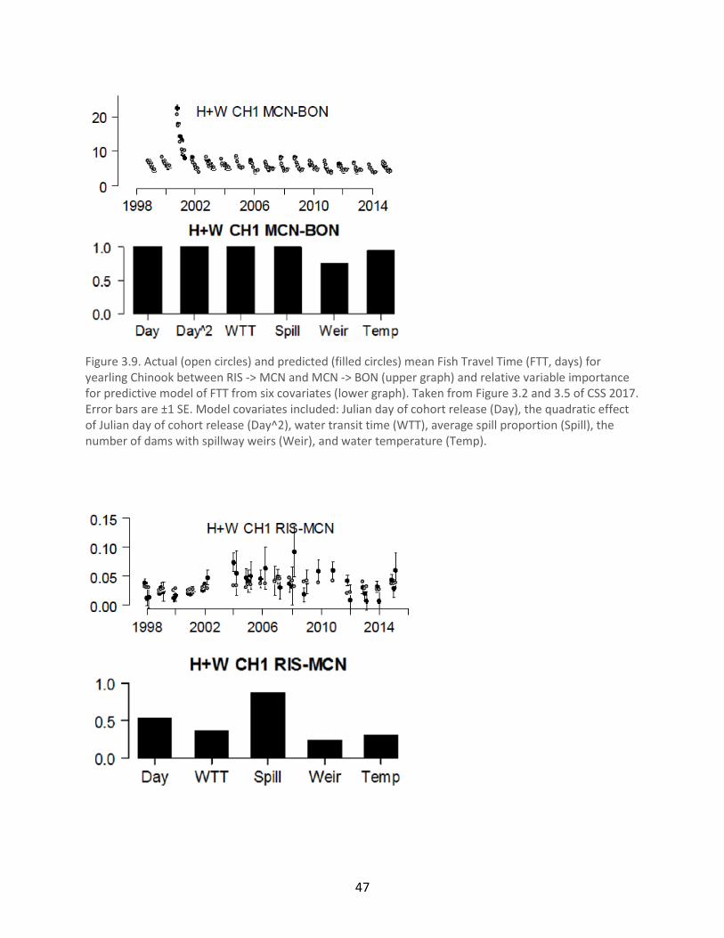
47
Figure 3.9. Actual (open circles) and predicted (filled circles) mean Fish Travel Time (FTT, days) for yearling Chinook between RIS -> MCN and MCN -> BON (upper graph) and relative variable importance for predictive model of FTT from six covariates (lower graph). Taken from Figure 3.2 and 3.5 of CSS 2017. Error bars are ±1 SE. Model covariates included: Julian day of cohort release (Day), the quadratic effect of Julian day of cohort release (Day^2), water transit time (WTT), average spill proportion (Spill), the number of dams with spillway weirs (Weir), and water temperature (Temp).

48
Figure 3.10. Actual (open circles) and predicted (filled circles) for Instantaneous Mortality for yearling Chinook between RIS -> MCN and MCN -> BON (upper graph of pair) and variable importance (lower graph of pair). Taken from Figures 3.3 and 3.6 of CSS 2017. Error bars are ±1 SE. Model variables included: Julian day of cohort release (Day), water transit time (WTT), average spill proportion (Spill), the number of dams with spillway weirs (Weir), and water temperature (Temp).
Figure 3.11. Actual (open circles) and predicted (filled circles) of in-river survival for yearling Chinook between RIS -> MCN and MCN -> BON. Take from Figure 3.4 of CSS 2017. Error bars are ±1 SE. Variable importance plots not given in CSS 2017. In-river survival was estimated by developing models for travel time (FTT) and for instantaneous mortality (Z) and then combining the estimates using S = exp(- Z * FTT). Consequently, variable importance plots are not applicable.

49
Figure 3.12. SARs (including jacks) for MCN-BON (upper graph) and RRE-BON (lower graph) for Upper Columbia spring Chinook with confidence intervals computed using bootstrapping. Taken from Figure 4.14 and 4.15 of CSS 2017. Migration year 2014 is complete through 2-salt returns only.

50
Figure 3.13. Spring out-migrants’ yearling spring Chinook juvenile survival from RIS to MCN (top graph). These are 2-week Cormack-Jolly-Seber estimates for smolts captured, PIT-tagged, and released at RIS as part of the SMP project (FPC 2015 annual report). The confidence interval plotted is 95%. The geometric means (through 2014) noted by the horizontal dashed line are 0.61 and 0.59 for Chinook. Taken from Figure 4.17 of CSS 2017. Lower graph is overall SARs (including jack, RIS-BOS). Taken from Figure 4.18 of CSS 2017.
3.1.4.2. Influence of Harvest on Upper Columbia River Spring Chinook Salmon
Commercial harvest of Upper Columbia River salmon and steelhead exceeded 85% of returning
adults in the 1930s and 1940s (Mullan 1987). UCR spring Chinook are still harvested both in the
ocean and lower river fisheries (NMFS 2016), though harvest of UCR spring Chinook in ocean
fisheries appears to be low based on coded wire tag recovery. A non-selective tribal fisheries
and selective sport harvest for spring Chinook occur in the lower Columbia River. A non-

51
selective sport fishery for Chinook was opened above Priest Rapids Dam in 2002 but was
modified to a selective fishery in 2014 to limit harvest of spring Chinook. The United States v.
Oregon Management Agreement manages and coordinates ocean and in-river harvest in the
Columbia River Basin under the jurisdiction of the federal court. Regional co-managers set
annual harvest levels based on abundance of returning adult Chinook salmon (Table 3.3).
Table 3.3. Harvest rates for Chinook salmon in the Columbia River during the spring harvest season (presented to ISAB by Jeromy Jording, NOAA Fisheries).
There have been no integrated assessments of limiting factors, including harvest, across the full
range of the life history of spring Chinook salmon. Life-cycle models recently provided initial
analyses of the relative effect of harvest on returning adult spring Chinook salmon. The life-
cycle model for the Wenatchee basin evaluated a scenario of reduced harvest and found that
harvest effects were less than those of estuarine adult survival and hatchery operations
(Jorgensen et al. 2017). Recent modeling analysis of competing tradeoffs between marine
mammal predation and fisheries harvest of Chinook salmon found that predators in the lower
river and ocean affected survival more than fisheries harvest (Chasco et al. 2017).
3.1.5. Limiting Factors Conclusions
The Upper Columbia Salmon Recovery Board (UCSRB) has refined its analysis of limiting factors
substantially since the first assessments in the late 1990s. The scientific principles for

52
identifying factors limiting the recovery of Upper Columbia spring Chinook salmon are generally
sound. Limiting factors are defined in the Recovery Plan of the Upper Columbia Salmon
Recovery Board (UCSRB) as environmental conditions that negatively affect the abundance,
productivity, spatial structure, and diversity of salmon populations. Analysis of limiting factors
based on current habitat conditions is useful for prioritizing restoration actions. The UCSRB
recently refined their traditional habitat-based approaches by weighting limiting factors based
on anticipated survival benefits and geographic extent. Assessments of limiting factors are used
to prioritize recovery actions, and the recent history of restoration is relatively consistent with
the rankings of limiting factors.
Analysis of potential limiting factors based on current habitat conditions in the basins that
contain natal streams is a useful context for planning and prioritizing restoration actions, but it
does not incorporate:
population dynamics of the fish and assessment of risk of extinction
the full life history of the fish and their geographic range from egg to adult spawner
temporal variation and climate change
hatchery effects
hydrosystem effects
in-river and ocean harvest
predation
out-of-basin management actions
Limiting factors analysis based on current habitat conditions is useful for prioritizing restoration
actions. The UCSRB recently refined their traditional habitat-based approaches by weighting
limiting factors based on anticipated survival benefits and geographic extent. To date, analysis
has focused on limiting factors related to habitat conditions. The limitations of four Hs on spring
Chinook populations are considered in isolation. Limiting factors analyses of the headwater
basins do not incorporate the full life history of the fish and their geographic range from egg to
adult spawner. Limiting factors for spring Chinook salmon in the Upper Columbia have been
assessed through traditional freshwater habitat assessments, analysis of density dependence,
and life cycle models. These methods are complementary rather than mutually exclusive. Each
have important applications in management of the four Hs, but to date there has been no
integration of all three approaches.
Empirical density dependence data and life-cycle modeling conducted by regional scientists in
the Upper Columbia provide more holistic analyses of limiting factors over the full life cycle of
spring Chinook salmon than traditional assessments of habitat-related limiting factors in
freshwater. These traditional habitat-based approaches can be used in planning and prioritizing
restoration actions, but more explicit integration of these approaches would strengthen future
efforts. As an example, monitoring data in the Okanogan basin is incorporated into an EDT
model, which includes a life-cycle model.

53
The UCSRB program’s goal is to identify limiting factors within four categories of human
impacts (threats), including habitat, harvest, hydrosystem, and hatcheries (four Hs), both within
and outside the Upper Columbia watershed. While the Recovery Plan recognizes the influence
of all Hs, analysis of limiting factors has not integrated the four Hs to determine which have the
greatest influence on spring Chinook populations. Life-cycle models for these subbasins are
beginning to provide evidence that addresses all Hs, but they are in early stages of
development. Limiting factors are considered to be working hypotheses that can be tested, and
monitoring and adaptive management are critical for understanding and addressing them. Key
uncertainties such as ocean productivity and global climate change are identified.
3.2. Comparison of Upper Columbia River Spring Chinook Recovery with Snake River Spring Chinook Recovery
The Oversight Panel asked the ISAB to compare the recovery of Upper Columbia River Spring
Chinook (UCRSC) to that of Snake River Spring Chinook (SNRSC). The ISAB believes that despite
geographic and biological differences in the two systems and the fact that only 10 years have
passed since completion of the UCRSC recovery plan (Upper Columbia Salmon Recovery Board
2007), this comparison may provide insights into recovery of UCR spring Chinook. Here we
describe the geographic and biological differences and similarities in the two ESUs and offer a
comparison of the recovery of spring Chinook in the two systems.
3.2.2. Geography
3.2.1.1. Spatial Structure
Population spatial structure describes how populations are arranged geographically based on
dispersal factors and quality of habitats (McElhany et al. 2000). There are three subbasins
containing extant populations in the Upper Columbia ESU amounting to about 940,000 hectares
(2.3 million acres), while the 26 subbasins in the Snake River ESU cover 11.5 million hectares
(28.3 million acres) (estimates include both current distribution and functionally extirpated
area). The ICTRT (2007) separated the populations into subbasin size categories and within
population complexity based on:
“A set of four population size categories (Basic, Intermediate, Large and Very
Large) for Interior basin stream type chinook… The smallest populations were
grouped into the Basic size category. Populations assigned to the Basic size
categories tended to be simple in complexity, often with a relatively linear
arrangement of spawning/rearing reaches. Median population size roughly
doubled between size categories. Populations with significantly higher amounts
of potential spawning habitat usually exhibited a higher degree of spatial
diversity—e.g., multiple tributary branches. Contemporary redd survey results

54
indicated that the distribution of spawners across sub-areas within a population
was likely to be patchy. Relatively high spawning concentrations in particular
sub-areas could be achieved in the larger, more complex population at lower
overall spawning densities… We used two methods to characterize the relative
within-population complexity of tributary spawning habitats—assigning each
population to one of four general structural complexity categories… and
estimating the number of relatively large, contiguous production areas within
each population... We defined a branch as a river reach containing sufficient
habitat to support 50 spawners. Major spawning areas (MaSAs) were defined as
a system of one or more branches that contain sufficient habitat to support 500
spawners... We defined contiguous production areas capable of supporting
between 50 and 500 spawners as minor spawning areas (MiSAs).” (ICTRT 2007,
pages 15-16).
Two of the three subbasins (66%) in the UCR (Table 3.4) are very large compared to just two
very large subbasins of 26 (8%) in the SNR (Table 3.5). The remaining SNR subbasins range in
size from basic to large. By virtue of the larger number of subbasins, the SNR has a broader
range of stream complexities (e.g., linear vs dendritic) than does the UCR; however, the UCR
tends to have more major (MaSA) and minor (MiSA) spawning areas per subbasin than does the
SNR (Tables 3.4 and 3.5).

55
Table 3.4. Intrinsic size and complexity ratings for historical populations within the Upper Columbia River Spring Chinook ESU. Organized by Major Population Groupings. Complexity categories: A = linear; B= dendritic; C= trellis pattern; D= core drainage plus adjacent but separate small tributaries (from ICTRT 2007a, page 20).
Table 3.5. Intrinsic size and complexity ratings for extant Snake River Spring Chinook ESU populations organized by Major Population Groupings. Complexity categories: A = linear; B=dendritic; C= trellis pattern; D= core drainage plus adjacent but separate small tributaries. Underlined entries represent a change from the previous designation. Size categories in parentheses represent core tributary production areas (page 17, ICTRT, 2007a).
Major Population
Group
Weighted Area
Category
Complexity
Population Category
#MaSA (#MiSA)
Lower Snake Tucannon R
Asotin R. (ext)
Intermediate
Basic
A
A 1 (0) 0 (1)
Grande
Ronde/Imnaha R
Lostine/Wallowa R.
Upper Grande Ronde R.
Catherine Creek
Imnaha R. Mainstem
Minam R.
Wenaha R.
Big Sheep Cr. (ext)
Lookingglass Cr. (ext)
Large
Large
Large
Intermediate
Intermediate
Intermediate
Basic
Basic
B
B
B
A
A
A
A
A
3 (1) 3 (2)
2 (2)
1 (1) 2 (0)
1 (0)
0 (1)
0 (1)
South Fork Salmon
South Fk Mainstem
Secesh R.
East Fk/Johnson Cr.
Little Salmon R.
Large
Intermediate
Large
Inter. (Basic)
C
A
B
D
2 (2) 1 (1)
2 (0)
0 (3)

56
Middle Fork Salmon
Big Creek
Bear Valley
Upper Mainstem MF
Chamberlain Cr.
Camas Creek
Loon Creek
Marsh Creek
Lower Mainstem MF
Sulphur Creek
Large
Intermediate
Intermediate
Inter. (Basic)
Basic
Basic
Basic
Basic
Basic
B
C
C
D
B
C
C
A
A
3 (0) 3 (0)
1 (2)
1 (3) 1 (1)
1 (0)
1 (0)
0 (1)
1 (0)
Upper Salmon
Lemhi Lower Mainstem
Pahsimeroi
Upper Salmon East Fk
Upper Salmon Mainstem
Valley Cr.
Yankee Fork
North Fork Salmon R.
Panther Cr. (ext)
Very Large
Very Large
Large
Large
Large
Basic
Basic
Basic
Intermediate
B
C
B
C
C
A
C
D
C
3 (2) 3 (5)
5 (0)
1 (0) 3 (0)
1 (0)
1 (0)
1 (0)
1 (2)
The more restricted geographic area of the UCR results in very homogeneous spawning
elevations—ranging from about 1600 to 3000 feet—as opposed to the SNR where spawning
areas are available up to 7000 feet (Figure 3.14). The UCR subbasins are located on the eastern
slopes of the Cascade Mountains and receive between 25 to 55 inches of precipitation annually
(Figure 3.15). The SNR is in the more arid eastern portion of the Columbia Basin, and SNR
subbasins tend to receive less precipitation than those in the UCR (Figure 3.15). Hydrologic
regimes in subbasins of both ESUs are a mix of rain, transition, and snow (Figure 3.16). The
CHaMP assessment of the geomorphic condition is similar for the subbasins; however, UCR
subbasins may contain a larger percent of intact and good areas than the SNR subbasins (Figure
3.17).
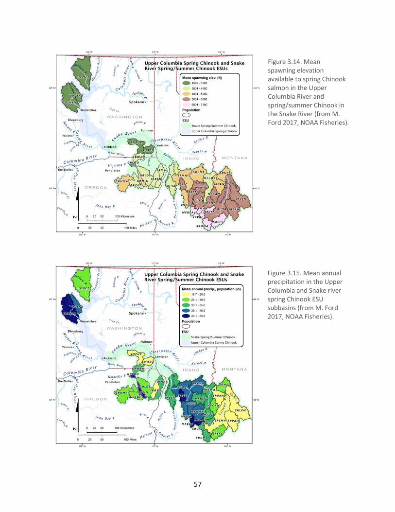
57
Figure 3.14. Mean spawning elevation available to spring Chinook salmon in the Upper Columbia River and spring/summer Chinook in the Snake River (from M. Ford 2017, NOAA Fisheries).
Figure 3.15. Mean annual precipitation in the Upper Columbia and Snake river spring Chinook ESU subbasins (from M. Ford 2017, NOAA Fisheries).

58
Figure 3.16. Hydrologic regime of Upper Columbia spring Chinook and Snake River spring/summer Chinook ESUs (from M. Ford 2017, NOAA Fisheries).
Figure 3.17. Geomorphic condition based on CHaMP analyses of subbasins of ESUs in the Upper Columbia River (three on the right) and representative subbasins in the Snake River (three on the left). Figure provided by M. Ford 2017, NOAA Fisheries with data from C. Jordan.

59
3.2.1 Comparison of Population Diversity
3.2.2.1 Life History and Genetic Diversity
Population diversity consists of the underlying genetic and life history characteristics that
provide for population resilience and persistence across space and time (McElhany et al. 2000).
Differences in the two ESUs may result in less population diversity in the UCR than the SNR.
There are only three extant populations of spring Chinook in the Upper Columbia compared to
26 populations in the Snake River. Furthermore, the SNR ESU includes summer Chinook while
summer Chinook in the UCR are not listed under the Endangered Species Act (ESA). Waples et
al. (2004) reported that interior Columbia Basin Chinook salmon were closely related based on
a yearling (stream-type) emigration life history. Additionally, yearling (stream-type) spring and
summer Chinook have an ocean migration that differs from subyearling (ocean-type) emigrants
that are readily harvested in the ocean (Myers et al. 1998). Genetic differences among Chinook
populations are more strongly correlated to yearling life-history strategy and marine
distribution than to spawning-run timing (Waples et al. 2004). Thus, the UCR summer Chinook
are genetically more similar to UCR fall Chinook than UCR spring Chinook, while SNR summers
are more genetically similar to springs than non-listed fall or summer Chinook in the mid and
Upper Columbia River (Narum et al. 2010, Waples et al. 2004, NMFS 2015). At the time of ESA
listing, the UCR spring Chinook were listed as endangered while spring Chinook in the SNR were
listed as threatened (Ford et al. 2015). This suggests that the UCR spring Chinook populations
were at a higher risk of extinction at the time of listing than were the SNR populations. These
ESA designations continue today.
Genetic research published recently (Johnson et al. 2018) concludes that contemporary
populations of Chinook salmon, including those originally from areas above Grand Coulee Dam,
have less genetic diversity compared to ancient Chinook present in the Columbia Basin 300 to
7600 years ago. Losses of genetic diversity occur when population size diminishes and
geographic range size contracts over time. Snake River Chinook salmon populations do not
appear to have experienced the same degree of loss of genetic diversity over time because
comparative changes in abundance and distribution are not as pronounced as those in the UCR
(Johnson et al. 2018). Based on genetic differences, the groups also differed demographically
with the UCR Chinook having experienced a reduction in effective population size, while the
SNR Chinook have not. The study included fall-, spring- and summer-run fish, and the authors
suggest that their findings could be the result of differing genetic contributions of the runs and
the cumulative effects of exploitation by native and non-native fishers both pre- and post-
European immigration to North America (Johnson et al. 2018).
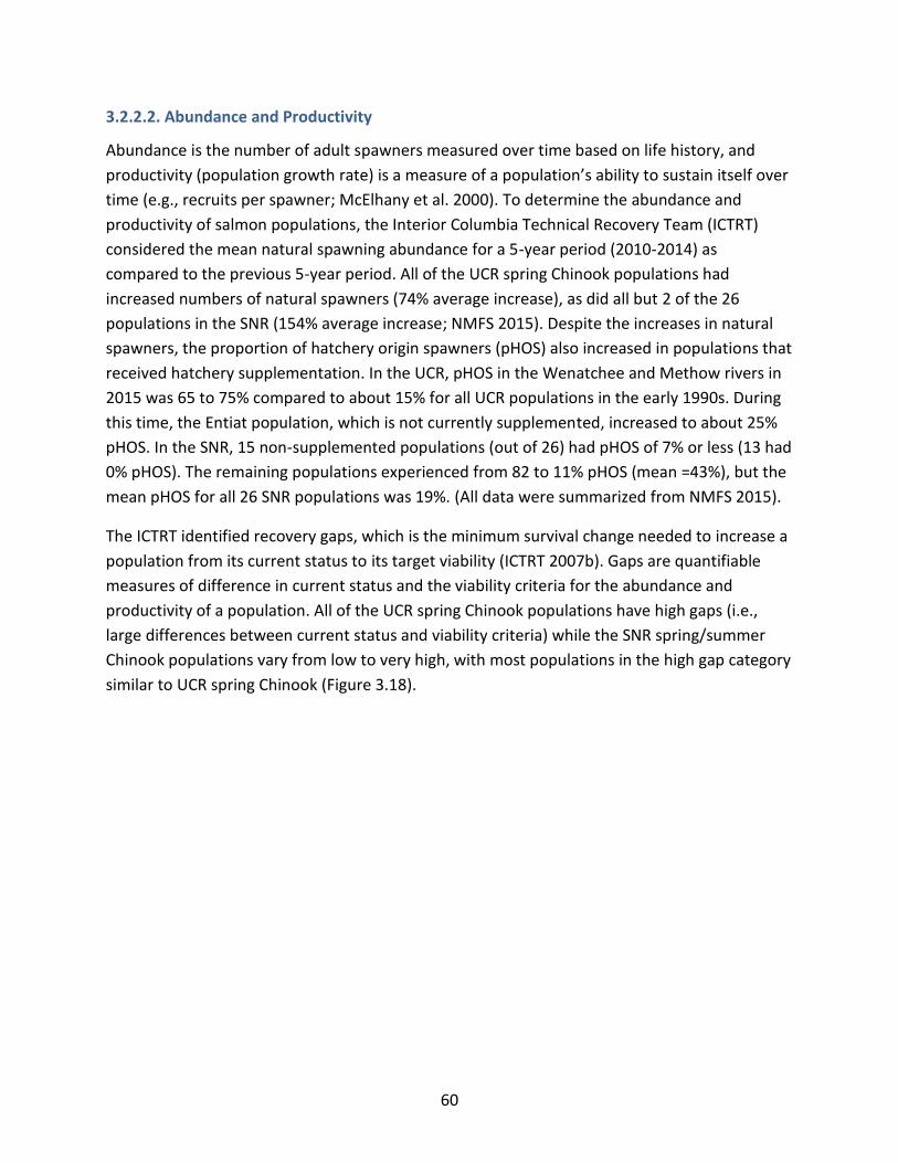
60
3.2.2.2. Abundance and Productivity
Abundance is the number of adult spawners measured over time based on life history, and
productivity (population growth rate) is a measure of a population’s ability to sustain itself over
time (e.g., recruits per spawner; McElhany et al. 2000). To determine the abundance and
productivity of salmon populations, the Interior Columbia Technical Recovery Team (ICTRT)
considered the mean natural spawning abundance for a 5-year period (2010-2014) as
compared to the previous 5-year period. All of the UCR spring Chinook populations had
increased numbers of natural spawners (74% average increase), as did all but 2 of the 26
populations in the SNR (154% average increase; NMFS 2015). Despite the increases in natural
spawners, the proportion of hatchery origin spawners (pHOS) also increased in populations that
received hatchery supplementation. In the UCR, pHOS in the Wenatchee and Methow rivers in
2015 was 65 to 75% compared to about 15% for all UCR populations in the early 1990s. During
this time, the Entiat population, which is not currently supplemented, increased to about 25%
pHOS. In the SNR, 15 non-supplemented populations (out of 26) had pHOS of 7% or less (13 had
0% pHOS). The remaining populations experienced from 82 to 11% pHOS (mean =43%), but the
mean pHOS for all 26 SNR populations was 19%. (All data were summarized from NMFS 2015).
The ICTRT identified recovery gaps, which is the minimum survival change needed to increase a
population from its current status to its target viability (ICTRT 2007b). Gaps are quantifiable
measures of difference in current status and the viability criteria for the abundance and
productivity of a population. All of the UCR spring Chinook populations have high gaps (i.e.,
large differences between current status and viability criteria) while the SNR spring/summer
Chinook populations vary from low to very high, with most populations in the high gap category
similar to UCR spring Chinook (Figure 3.18).

61
Figure 3.18. Abundance and productivity gaps for Snake River Spring/Summer Chinook ESU populations (map also includes Upper Columbia Spring Chinook ESU populations for comparison). Populations with insufficient data to generate gaps shaded in gray. Gaps are defined as relative improvement in productivity or limiting capacity required for a population to exceed its corresponding 5% risk viability curve (ICTRT 2007b). Figure is from NMFS (2015).
It appears that changes in abundance and productivity of the two ESUs are similar and the
number of natural spawners have increased in both systems. However, on average, the
increase in SNR populations in 2010-2014 was twice that of UCR populations. The proportion of
hatchery origin spawners has also increased in hatchery supplemented populations in both
systems, but since the SNR has a number of populations that are not supplemented, the
average pHOS for all 26 SNR populations is less than half that of the average of the three UCR
populations.

62
3.2.2.3. Smolt Migration and Survival through the Hydrosystem
Freshwater spawning and rearing habitats of SNR spring/summer Chinook populations are
located upstream of Lower Granite Dam (LGR), and smolts must emigrate through four Snake
River hydropower dams before reaching the mainstem Columbia River upstream of McNary
Dam (MCN). The UCR spring Chinook populations emigrate into the Columbia mainstem and
pass three, four, or five dams before reaching the free-flowing Hanford Reach and subsequently
McNary Dam.
The Comparative Survival Study (CSS) tracks smolt migration and survival from Rock Island Dam
(RIS) in the UCR and from LGR in the SNR to MCN, and from MCN to Bonneville Dam (BON).
There are significant differences in the Chinook populations. The number of emigrants in the
UCR is significantly less than in the SNR. To have adequate sample sizes and thus adequate
statistical power, the CSS creates smolt cohorts of all fish passing a dam during a specific time
period. In the UCR, the cohorts are composed of all wild and hatchery spring Chinook detected
at RIS during a two-week period. In the SNR, wild and hatchery fish are in separate cohorts that
pass LGR during a one-week period. With these caveats in mind, the probability of UCR spring
Chinook smolts surviving (RIS to MCN) is about 60%, while SNR smolt probability of survival
(LGR to MCN) is about 75 to 80% (Figure 3.19). It is important to note that the CSS reported that
“within-year estimates of (survival) varied by up to 39 percentage points for both wild yearling
Chinook and steelhead, and by up to 32 percentage points for hatchery yearling Chinook” (CSS
2017 Draft). As a result, they were not able to model the role of environmental factors on
survival. Faulkner et al. (2017) calculated the probability of survival for smolts emigrating from
hatcheries in the UCR and SNR to dams in the Columbia River beginning in the 1990s (Table
3.6). This study included mortalities from hatcheries in the tributaries to the dams. The results
are very similar to those reported by CSS (2017) but also suggest the possibility that UCR smolts
had better survival than the SNR smolts when the full emigration from hatchery to BON is
considered (Faulkner et al. 2017).

63
Figure 3.19. Estimates of in-river survival probability for release cohorts of hatchery (H) and wild (W) yearling Chinook salmon (CH1) migrating in the LGR–MCN and RIS–MCN reaches, 1998–2016. The error bars represent +/- 1 SE. Figure was provided by J. McCann, FPC and was derived from the CSS 2017 Draft.

64
Table 3.6. Probability of smolt survival when migrating from hatcheries in the Upper Columbia River (UCR) or the Snake River (SNR) to either Lower Granite Dam (LGR) or McNary Dam (MCN) and from MCN to Bonneville Dam (BON). Values are the means (SE) for the migration years listed. Data are from Faulkner et al. (2017). The ISAB derived values for Hatchery-BON by multiplying the mean values for the reaches.
Smolt Survival
ESU Reach Years Probability (SE) Hatchery-
BON
UCR Hatchery-MCN 1999-2016 0.555 (0.012) MCN-BON 0.809 (0.034) 0.449 SNR Hatchery-LGR 1993-2016 0.629 (0.012) LGR-MCN 0.736 (0.013)
MCN-BON 0.703 (0.021) 0.325
It is possible that avian and fish predation may be the cause of significant UCR Chinook
mortality (McMichael et al. 2017). However, comparing data from different years (i.e., 2012 and
2014), it appears that that yearling Chinook migrating from RIS through the Hanford Reach did
not experience any more avian predation, as a part of total mortality, than did yearling Chinook
migrating in the lower Snake River (Table 3.7; Evans et al. 2015, 2016). Based on existing data, it
is not possible to detect differences in smolt survival during their emigration from the UCR to
BON versus SNR to BON.
Table 3.7. Reach-specific bird predation rates (percentage of tagged fish consumed, as means with SE) and total mortality of tagged yearling Chinook salmon released into the mid/Upper Columbia River at river kilometer 729 in 2014 (bottom) or into the lower Snake River at river kilometer 562 in 2012 (top). Five-weekly releases started on 30 April 2012 and 24 April 2014. Data from Evans et al. (2015).
3.2.2.4. Smolt-to-Adult Returns
NMFS (2015) considered smolt-to-adult returns (SARs) from several ESA-listed salmonids in the
Columbia River Basin including UCR natural origin spring Chinook and SNR spring/summer
Chinook. These data were rescaled to three-year moving averages to reduce the impact of
short-term climate variability and relied on a long data series of smolt and adult natural-origin
spring Chinook in the Chiwawa River (Figure 3.20). All of the populations have similar patterns,
with low SARs in 1990s and peaks in the early 2000s (NMFS 2015).
Bird Predation Total Mortality Bird Predation Total Mortality % Total
2012 3.7% (1.7-7.2) 8.9% (8.7-8.9) 42.70%
2014 2.8% (1.0 - 5.9) 12.2% (11.3-12.6) 29.50%NA
UCR (Rkm 729-545) SNR (Rkm 562-525)
NA
65
The CSS calculates SARs for UCR spring Chinook smolts passing Rocky Reach Dam (RRE) to their
detection as adults at Bonneville Dam adult collection facility (BON-A). Snake River
spring/summer Chinook SARs are calculated from LGR to BON-A. The CSS calculates SARs for
individual hatcheries in both systems and also for the natural origin UCR spring Chinook (from
the Entiat and Methow rivers) and SNR natural origin spring/summer Chinook. SARs for these
groups of fish along with natural origin Wenatchee River spring Chinook are also calculated for
smolts passing McNary Dam (MCN) and returning to BON-A. Comparing the natural origin
Chinook groups is more appropriate than comparing the SARs from 3 UCR hatcheries with 10
SNR hatcheries. Furthermore, complete SNR data are from 2000 through 2014, as compared to
UCR data from 2008 through 2014. Here we considered this overlapping 7-year period and
found SARs for natural origin UCR spring Chinook did not differ from those of the natural origin
SNR spring/summer Chinook (Table 3.8). Thus, since the UCR recovery plan has been in place
(UCSRB 2007), there has been no difference in SARs of natural origin UCR spring Chinook
compared to that of natural origin SNR spring/summer Chinook.

66
Figure 3.20. Snake River spring/summer Chinook salmon aggregate smolt to adult return rates (solid blue), Upper Columbia spring Chinook (blue dashed line). Each SAR series is rescaled by dividing annual values by the corresponding series mean to facilitate relative comparison. (Figure and caption derived from NMFS 2015).

67
Table 3.8. Smolt-to-adult return rate for Upper Columbia River (UCR) natural origin spring Chinook salmon (Sp Chin) and Snake River (SNR) natural origin spring/summer Chinook (Sp/Su Chin) that passed Lower Granite Dam (LGR), Rocky Reach Dam (RRE) or McNary Dam (MCN) and were subsequently detected at Bonneville Dam (BOA) as returning adults (jacks included). The UCR fish come from the Entiat (Ent), Methow (Met) or Wenatchee (Wen) river. P-value is based on a t-test with unequal variances; data for the Wenatchee were not included in statistical analysis. Data are summarized from CSS (2017 draft, Appendix B).
Smolt-to-Adult Returns
LGR-BOA RRE-BOA
MCN - BOA
Brood Year SNR
Sp/Su Chin
UCR
Sp Chin (Ent +
Met)
SNR
Sp/Su Chin
UCR
Sp Chin (Ent +
Met)
UCR
Sp Chin
(Wen)
2008 4.13 1.72
4.07 3.26 2.89
2009 2.09 1.20
2.00 2.40 2.07
2010 1.16 1.21
1.28 1.97 1.70
2011 0.45 0.44
0.46 0.62 1.02
2012 1.84 1.03
2.32 1.77 1.14
2013 1.71 1.66
1.69 2.80 1.93
2014 0.68 1.07
0.43 1.87 1.11
Mean 1.72 1.19 1.75 2.10 1.69
SD 1.22 0.43 1.25 0.85 0.67
SE 0.17 0.06 0.18 0.12 0.10
P(t-test) 0.16 0.28
3.2.2.5. Adult Mortalities in the Columbia River
3.2.2.5.1. Harvest
Exploitation rates (total harvest) for UCR spring Chinook are the same as those for the SNR
spring/summer Chinook and have been averaging about 10% since 1980 (NMFS 2015).
However, the rate for both ESUs appears have been increasing since 2000 (Figure 3.21).

68
Figure 3.21. Exploitation rate (total harvest) for Upper Columbia River spring Chinook salmon. As reported in NMFS 2015, the exploitation rates for Snake River spring/summer Chinook were identical. Data are from Columbia River Technical Advisory Committee. Figure is from NMFS (2015).
3.2.2.5.2. Pinniped Predation
Researchers from NOAA-Fisheries have been investigating adult salmon migration timing and
pinniped predation in the lower Columbia River. Sorel et al. (2017) cites Rub et al. (in
preparation) as saying that survival of adult salmon migrating from Astoria to BON decreased
between 2010 and 2015 and that survival is lowest in the fish migrating earliest in the season.
These measures of survival coincide with increases in pinnipeds in the lower river. Sorel et al.
(2017) documented the passage times of UCR and SNR adults at BON from 1998 through 2015
(Figure 3.22). There is significant overlap in the UCR and SNR spring-run Chinook passage.
However, summer-run fish—which are part of the SNR ESU, but not the UCR ESU—arrive later
and potentially would not be preyed upon to the extent of the spring-run Chinook.
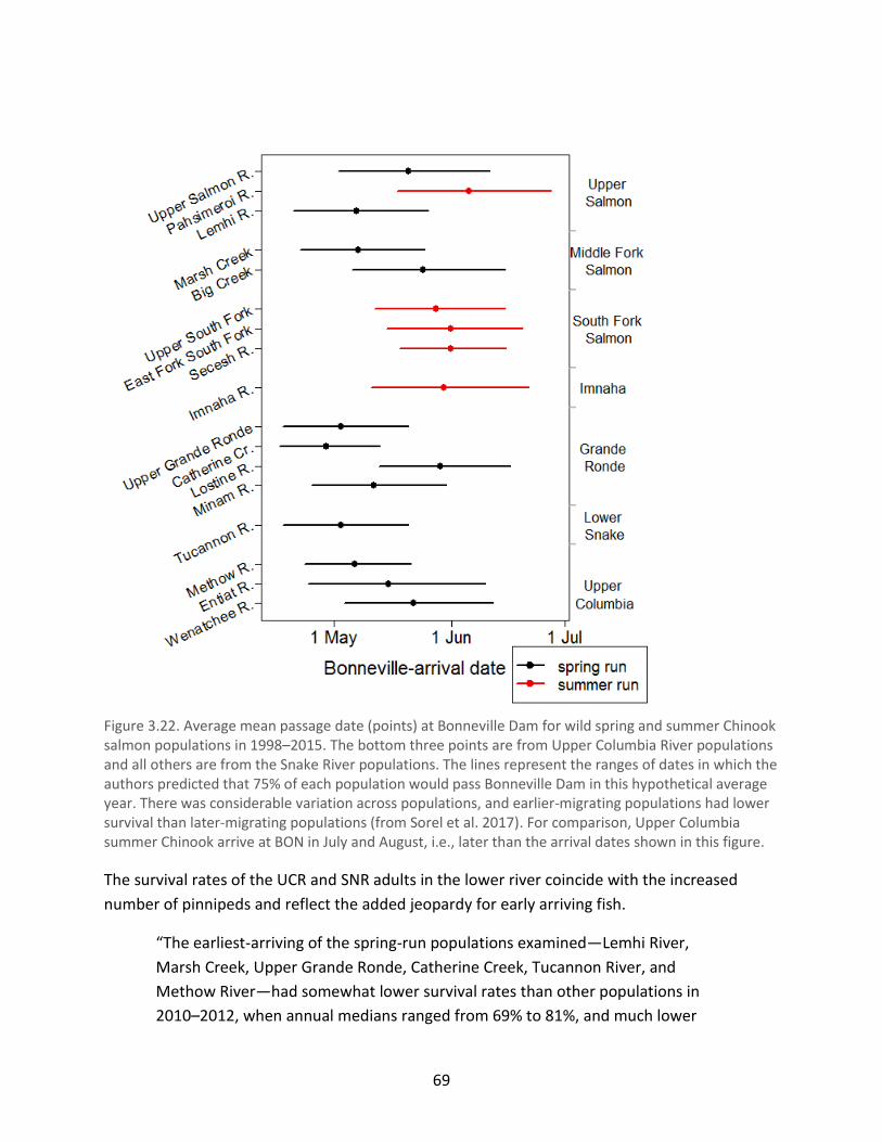
69
Figure 3.22. Average mean passage date (points) at Bonneville Dam for wild spring and summer Chinook salmon populations in 1998–2015. The bottom three points are from Upper Columbia River populations and all others are from the Snake River populations. The lines represent the ranges of dates in which the authors predicted that 75% of each population would pass Bonneville Dam in this hypothetical average year. There was considerable variation across populations, and earlier-migrating populations had lower survival than later-migrating populations (from Sorel et al. 2017). For comparison, Upper Columbia summer Chinook arrive at BON in July and August, i.e., later than the arrival dates shown in this figure.
The survival rates of the UCR and SNR adults in the lower river coincide with the increased
number of pinnipeds and reflect the added jeopardy for early arriving fish.
“The earliest-arriving of the spring-run populations examined—Lemhi River,
Marsh Creek, Upper Grande Ronde, Catherine Creek, Tucannon River, and
Methow River—had somewhat lower survival rates than other populations in
2010–2012, when annual medians ranged from 69% to 81%, and much lower

70
survival rates in 2013–2014, which had a 50–70% range in annual median
survivals. Populations with intermediate run timing such as the Upper Salmon
River, Big Creek, Minam River, Entiat River, and Wenatchee River had
experienced survival that was somewhat lower in 2013–2015, with annual
medians of 67–85%, than 2010–2012’s 79% to 88% range. Late-arriving
populations—Pahsimeroi River, Upper South Fork Salmon River, East Fork South
Fork Salmon River, Secesh River, Imnaha River, and Lostine River—most of which
are considered summer-run, had the highest survival rates with the least
interannual variability” (Sorel et al. 2017, page 14).
Sorel et al. (2018) recently indicated that average survival in the lower Columbia River (i.e.,
below BON) in 2013-2015 was 13% lower than in 2001–2012 for the Methow River population.
The Entiat River population experienced an 8% decline in survival between these periods, and
survival of the Wenatchee River population was 4% lower (Sorel et al. 2018). The extent of this
decreased survival correlates with the timing of arrival of these populations at BON (see Figure
3.11 in section 3.3.). The question of pinniped predation is also addressed in Section 3.4.
Pinniped Predation (below).
3.2.2.5.3. Pre-spawning Mortality (PSM)
Over the past 16 years, an average of 46% of the UCR spring Chinook females died prior to
spawning as compared to 15% of the UCR summer Chinook (Murdoch, 2017). A variety of
sources suggest that annual pre-spawning mortality of spring/summer Chinook in the SNR is
more like the UCR summer Chinook than the UCR springs. Cleary et al. (2014) reported PSM
averaged 16% for natural origin Chinook spawners in the Lostine River between 2002-2012;
Crump et al. (2017) reported the same 16% pre-spawning mortality for Chinook in the
Lookingglass Creek from 2004-2016. The variance of the reported pre-spawning mortality in
both SNR subbasins is high with the Lostine varying from 5% to 32% and Lookingglass ranging
from 0 to 54%.
3.2.2.6. Ocean and Estuary
The ISAB reviewed relevant scientific information on smolt-to-adult estuary and ocean life
history traits and population status indicators (see Appendix B), and concluded that UCR spring
Chinook and SNR spring/summer Chinook ESUs exhibit similar estuary-ocean life histories and
thus are likely to experience similar limiting factors in these habits. However, the ISAB found
large gaps in scientific knowledge and understanding of estuary-ocean life histories and
associated limiting factors for both ESUs. For example, there is a nearly complete absence of
data on seasonal and spatial distribution, abundance, and survival both during and after the
first winter at sea. Most of the available population-specific data for both ESUs are for
hatchery-origin fish, which do not always exhibit life history traits and population dynamics of

71
natural-origin conspecifics. Our review found that hatchery-origin fish differed between the two
ESUs in key traits that could influence marine ecological interactions (e.g., predation,
competition) and ocean growth and survival (e.g., smolt abundance and size at release, and
ocean distance traveled before offshore dispersal). As we discussed in section 3.1, analysis of
potential limiting factors based on current freshwater habitat conditions in natal basins is a
useful context for planning and prioritizing habitat restoration actions in the UCR but does not
account for the potential effects of highly variable out-of-basin factors, such as ocean
conditions, on abundance, survival, diversity, and extinction risk of UCR spring Chinook salmon.
The ISAB suggests that a practical approach to addressing and identifying estuary-ocean
information gaps and limiting factors for UCR spring Chinook would be to coordinate and
collaborate in this effort with the Council’s Plume and Ocean Science Forum (assuming some
form of that valuable forum continues to meet) and international treaty programs aimed at
addressing these issues, such as the Pacific Salmon Commission, North Pacific Anadromous Fish
Commission, North Pacific Fisheries Commission, and North Pacific Marine Sciences
Organization (PICES).
The ISAB considers the NOAA “Module for the Ocean Environment” (NOAA 2014) to be a highly
relevant document for the current review. The NOAA Ocean Module was developed to support
integrated recovery plans for four SNR ESUs including the spring/summer Chinook ESU. The
document summarizes recent (through 2014) scientific information on estuary-ocean life
history and ecology of SNR spring/summer Chinook and anthropogenic risks to this ESU during
the estuary-ocean life stages. In the context of recovery planning and implementation, NOAA
(2014) provides compelling reasons for addressing potential limiting factors during estuary and
ocean life stages. For example, the tidal freshwater/estuary/plume/ocean survival of yearling
hatchery-origin SNR spring Chinook is highly correlated with the overall smolt-to-adult survival
ratio (SAR) but not with in-river survival during the outmigration year (2000-2009). Thus, for
example, the negative effects of poor estuary-ocean conditions on SARs might mask any
positive effects of freshwater habitat restoration in the basin. The document also addresses key
information needs, recovery strategies, adaptive recovery actions based on ocean conditions,
and monitoring and research needs from the perspective of recovery planning (NOAA 2014).
The ISAB recommends development and implementation of a similar ocean module for the UCR
spring Chinook ESU.
3.2.2.7. Limiting Factors and Ecological Concerns
Comparing factors limiting the abundance of two listed but widely separated runs of salmon
with similar life histories can provide insights for managers (Section 3.1.1). However,
comparisons between UCR spring Chinook ESU and SNR spring/summer Chinook ESU should be
regarded with a degree of skepticism because of physical, chemical, and biological differences

72
between the watersheds, differences among tributaries within watersheds, and differences in
the evolutionary history of the two runs.
To isolate the effects of limiting factors, we assume that limiting factors outside the two regions
act in a similar fashion on both runs: both presumably experience similar ocean conditions,
similar predation issues in the estuary, and similar problems passing big dams and reservoirs in
the lower river, including predation by non-native fishes. Emigrating UCR spring Chinook must
pass three to five dams and SNR spring Chinook pass four before reaching McNary Dam, so
dams are roughly equivalent as sources of mortality. A complicating factor not adequately
considered in this comparison is the potentially complex role of hatchery fish as a limiting
factor. Hatcheries produce fish that can potentially compete for resources in both regions, but
their relative impacts are not discussed here. We assume that hatchery impacts in the two
basin are roughly equivalent, an assumption we acknowledge may be incorrect.
In the upstream areas in the two ESUs, most spawning and rearing takes place in tributary river
systems, so the limiting factors discussed here are mainly habitat factors in the tributaries. The
analysis of limiting factors in tributaries by the U.S. Bureau of Reclamation Remand Habitat
Workgroup (2015) is the basis for this comparison.
The analysis examined 21 factors related to habitat and gave them weighted importance ratings
for major tributaries/assessment units in each region. To provide a quick insight into similarities
and differences in limiting factors in the two regions, we compared the number of tributary unit
occurrences of significant ratings of impairment in habitat from the 21 factors in 2015 (n =30
tributary units for UCR spring Chinook and n=59 for SNRSC, Table 3.9). Factors important for
both regions were (a) water quantity, (b) sedimentation, (c) amount of instream habitat
complexity, (d) condition of riparian vegetation, and (e) effects of anthropogenic barriers.
Factors important to UCRSC but not to SNRSC included (a) altered primary production, (b)
condition of side channels and wetlands, (c) condition of floodplains, and (d) bed and channel
form. Factors important mainly to SNRSC were water temperature and recruitment of large
wood. The remaining 10 factors were not considered to be limiting for spring Chinook in most
areas of either region. What this analysis does not reflect is the variation among tributary units
in each region; each stream or site within a stream has its own particular challenges for spring-
run Chinook. Overall, this analysis should be regarded mainly as an indicator of the relative
importance of each factor for the purposes of comparison, with the numbers having little
meaning on their own.
The difficulty of rating limiting factors on a local scale is indicated by this statement by NMFS
(2016, page 47) that reflects the large-scale problems the SNRSC face:

73
“Both hydropower and land use activities have had significant impacts on habitat
in the mainstem Snake River above Lower Granite Dam. Twelve dams have
blocked and inundated habitat, impaired fish passage, altered flow and thermal
regimes, and disrupted geomorphological processes in the mainstem Snake
River. These impacts have affected juvenile and adult salmon and steelhead
through loss of historical habitat, altered migration timing, elevated dissolved
gas levels, juvenile fish stranding and entrapment, and increased susceptibility to
predation. In addition, land use activities, including agriculture, grazing, resource
extraction, and development have adversely affected water quality and
diminished habitat quality throughout this reach.”
Table 3.9. Comparison of limiting factors for Upper Columbia River spring Chinook salmon (UCRSC) with those for Snake River spring/summer Chinook salmon (SNRSC). Numbers of tributary units in which the factor is limiting (percent in parentheses) are based on ratings by experts for each factor, provided in www.onefishtwofish.net/viz/HabitatLimitingFactors1d. All of ratings in the top three (of five) categories were included in the total. For UCRSC, 30 tributary or management units were evaluated, while for SNRSC 59 tributary/management units were evaluated.
Factor UCRSC
# (%)
SNRSC
# (%)
Anthropogenic barriers 19 (63) 38 (64)
Habitat competition 0(0) 5(8)
Predation 0(0) 0(0)
Mechanical injury 0(0) 9 (15)
Altered primary production 14(47) 1(2)
Food, competition 0(0) 0(0)
Altered prey composition 0(0) 0(0)
Riparian vegetation 29(97) 40(68)
Large wood recruitment 0(0) 22(37)
Side channel, wetland conditions 16(53) 15(25)
Floodplain condition 21(70) 13(22)
Bed, channel form 28(93) 20(34)
Instream structural complexity 25(83) 37(63)
Decreased sediment quality 0(0) 1(2)
Increased sedimentation 17(57) 51(86)
Temperature 8 (27) 36(61)

74
Dissolved oxygen 0(0) 13(22)
Turbidity 0(0) 2(3)
Contaminants 0(0) 2(3)
Increased water quantity 0(0) 1(2)
Decreased water quantity 19 (63) 37 (63)
NMFS (2014) identified four major interrelated factors that limited viability of SNR
spring/summer Chinook salmon in the tributary systems: excess fine sediment, poor water
quality (primarily warm temperatures), low water quantity (primarily low summer flows), and
limited habitat quantity/diversity (primarily lack of deep pools and large wood). These factors
also become apparent in the analysis in Table 3.7 and are similar in both ESUs. Sediment, for
example, is a problem because runoff from surrounding lands is often laden with large
quantities of fine sediment that buries or cements the coarser sediment (gravel, cobbles)
needed for spawning by salmon. Excess sediment can also fill in pools and otherwise decrease
habitat diversity needed at all life stages. When water is diverted from the rivers, especially in
summer, capacity to flush or move sediment is reduced. Low flows also increase temperatures
in many stream reaches, further reducing their capacity to support salmon at diverse life history
stages.
In their five-year summary of spring Chinook status in the upper Columbia, NMFS (2016) stated,
“Despite significant efforts to improve habitat conditions, much of the habitat in
the range of UCR spring-run Chinook salmon...remains degraded. Restoring
habitat to historic conditions may not be needed to attain viability, but
considerable improvement is needed to restore habitat to levels that will
support viable populations of...spring-run Chinook salmon. In particular, the poor
status of the habitat is a major obstacle to achieving UCR spring-run Chinook
salmon ESU recovery.”
Barnas et al. (2015) compared ecological concerns in ESUs throughout the Columbia River Basin
using the data dictionary developed by Hamm (2012). Barnas et al. (2015) quantified ecological
concerns, which are about the same in the two ESUs in that SNR has some spring/summer
Chinook populations with fewer and some with more concerns than does UCR spring Chinook
populations (Figure 3.23).

75
Figure 3.23. Number of ecological concerns (please see text for definition) for the three Upper Columbia spring Chinook populations (yellow bars) and Snake River spring/summer Chinook populations (all other bars). Longer bars indicate more ecological concerns. Figure is from M. Ford 2017, NOAA-Fisheries with data from Barnas et al. (2015).
3.2.3. Conclusion for Snake River and Upper Columbia Chinook Comparison
Differences in geography and biology result in differences in the spatial structure and diversity
of the two evolutionarily significant units (ESUs). Nonetheless, most measures of population-
level abundance and productivity for spring Chinook and assessments of habitat are similar in
the two ESUs. In-river survival of spring Chinook smolts migrating in the Upper Columbia as
compared to Snake River spring/summer Chinook smolts, and smolt-to-adult survival (SAR) of
wild Upper Columbia and Snake River Chinook, do not appear to differ.
Because the Snake River ESU has many more populations and larger absolute abundance than
the Upper Columbia ESU, the consequences of the differences in relative proportions may be

76
worse for Upper Columbia spring Chinook than for Snake River spring/summer Chinook. If in-
river survivals are equal for the two ESUs, adverse events create greater risks for the Upper
Columbia populations because they are less buffered by adjacent populations. For example, if
the proportion of losses to pinniped predation continues to increase but are the same for the
two ESUs, the reduction of Upper Columbia spring Chinook spawners, which have smaller
numbers, might reduce their ability to find mates on the spawning grounds. Thus, the ISAB
believes that the Upper Columbia spring Chinook ESU may be exposed to greater risks than the
Snake River spring/summer Chinook ESU. The same concern was expressed when the Upper
Columbia ESU was originally listed as endangered and the Snake River ESU as threatened,
listings that were not changed in the most recent reviews (NMFS 2016a; 2016b).
3.3. Comparing the Abundance, Migration Timing, and Life History Strategies of Upper Columbia River Summer and Spring Chinook
During our site visit, Upper Columbia researchers indicated that the number of natural origin
summer Chinook returning to Upper Columbia subbasins was consistently greater than that
observed for spring Chinook. The question of why this might be the case was raised. The fish
are racial variants of the same species, therefore they are expected to be biologically similar.
Studies of the alternative life-history strategies of each race may provide important insights on
why Upper Columbia River summer Chinook are relatively successful while spring Chinook are
less so. Such differences could identify limiting factors for spring Chinook in the UCR subbasins,
and management actions could be developed to lessen their constraints on spring Chinook
abundance.
Andrew Murdoch (Washington Department of Fish and Wildlife) synthesized available data on
summer and spring Chinook returning to the Upper Columbia and presented this information to
the ISAB (Murdoch 2017). Much of this material was produced by the monitoring and
evaluation program funded by local PUDs (Chelan, Douglas, and Grant Counties). PUD scientists
also contributed to the presentation. Due to the availability of data, the comparisons made
were restricted to summer and spring Chinook returning to the Wenatchee, Methow, and
Okanogan subbasins. Fortuitously, U.S. Fish and Wildlife Service (USFWS) researchers have
been examining interactions between summer and spring Chinook in the Entiat River, which
also were presented to the ISAB by Tom Desgroseillier (Desgroseillier 2017).
The Murdoch presentation contrasted the two races of Chinook at distinct life-cycle stages,
based on differences observed for juveniles in freshwater, smolts before they enter the ocean,
and adults after they enter the Columbia River estuary. The USFWS study used genetic tools to
examine juvenile life history strategies of summer and spring Chinook salmon from the Entiat.

77
Life histories of UCR fish were compared to those observed in several other populations of
Upper Columbia Chinook salmon. Additionally, superimposition by summer Chinook on spring
Chinook redds and the possibility of hybridization between the two races in the Entiat subbasin
were evaluated.
3.3.1. Comparisons between Adult Summer and Spring Chinook Salmon
3.3.1.1. General Abundance Information
From 1989 to 2016, an average of 1,241 natural origin (NOR) spring Chinook have collectively
returned to the Wenatchee, Entiat, and Methow subbasins. During this time period no
temporal trend in spring Chinook abundance was detected (r2 = 0.002; p=0.83). During those
same return years, an average of 12,572 NOR summer Chinook returned to the Wenatchee,
Methow, and Okanogan subbasins. Even though summer Chinook exhibited a slight overall
increase in abundance (r2 = 0.142; p=0.048), numbers varied greatly (Figure 3.24). Additionally,
no temporal trend appears to exist in the percentage of spring Chinook returning to upper
Figure 3.24. The abundance of natural origin adult summer (black circles) and spring Chinook (open circles) returning to Upper Columbia River subbasins. Overall trends in abundance from 1989 – 2016 are shown for summer (solid line) and spring (dashed line) Chinook. From Murdoch (2017).
Columbia tributaries. This percentage has averaged 8.6% but is quite variable, ranging from a
low of 0.93% in 1995 when just 79 spring Chinook were counted to a high of 17.8% in 1993
when 2,179 returned.
Adult returns shown in Figure 3.24 do not include numbers of fish harvested in the Columbia
River or in ocean fisheries. A sport fishery and non-selective tribal fisheries for spring Chinook
occur in the lower river. In 2002, a non-selective sport fishery began for Chinook above Priest
Rapids Dam. This upriver fishery was changed to a selective fishery in 2014 to limit the harvest
0
5,000
10,000
15,000
20,000
25,000
1985 1990 1995 2000 2005 2010 2015 2020
Wild
Sp
awn
er
Ab
un
dan
ce
Return Year
78
of spring Chinook (Murdoch 2017). Addition of harvest numbers to the return values would
disproportionately increase abundance of summer Chinook, making the disparity in the current
abundance of naturally produced fish from these two races in the Upper Columbia even more
evident.
Summer Chinook have not always been the predominate race of Chinook returning to the
Upper Columbia. Counts of Upper River Columbia spring and summer Chinook began in 1933
after the Rock Island Dam was completed and have continued to the present day. The data we
were able to find did not separate hatchery from natural origin fish as was done in Figure 3.24.
Nevertheless, they show that the relative abundance of spring and summer Chinook in the
Upper Columbia has varied over time (Figure 3.25 A&B). In some years spring Chinook were
more abundant than summer Chinook. Perhaps the biggest change in relative abundance
between the two Chinook races occurred in the late 1990’s and early 2000’s.
The patterns of yearly abundance of NOR spring and summer Chinook in Figure 3.25 led to
three speculations. First, the substantial increase in NOR summer Chinook abundance in the
late 1990’s and early 2000’s was linked to the summer spill program that was initiated under
the 1995 BiOp. Second, the selective fishery started in 2014 has increased the abundance of
NOR spring Chinook. And finally, the abundance of both summer and spring Chinook NORs are
likely affected by some common factors. A weak but positive relationship (r2 = 0.20; p=0.017)
between the annual abundance levels of NOR spring and summer Chinook was detected when
return values were correlated with one another.

79
Figure 3.25 A&B. Counts of hatchery and natural origin adult summer (black circles) and spring Chinook (open circles) at Rock Island Dam from 1933 through 1968 (part A) and from 1973 through 2010 (part B). Jacks (3-yr-old males) are included in the counts made from 1933 to 1950. (Data are from Chelan PUD www.chelanpud.org/departments/yourPUD /RIAnnualFishCount.pdf)
0
20000
40000
60000
80000
100000
1970 1975 1980 1985 1990 1995 2000 2005 2010
Ad
ult
s C
ou
nte
d A
t R
ock
Isla
nd
D
am
Return Year
A
B

80
Return numbers can provide a general demographic overview of how population abundance
varies overtime, but grouping returns by brood year provides a number of important
advantages. Foremost among those is the development of recruitment curves that can
determine intrinsic productivity and the population carrying capacity in existing habitat (ISAB
2015-1). Additionally, smolt-to-recruit (SARs) estimates for each brood year can be made. SAR
values could be used to directly test the effects of the summer spill program on survival and
also allow a more refined assessment of how summer and spring Chinook abundance may be
related. The advantages of using brood year returns as opposed to annual returns have led us
to make several suggestions the researchers may wish to undertake if they are not already
underway:4
Add harvest values (by age) to the return numbers for years 1989 – 2016
Evaluate trends of abundance by brood year rather than by return year.
o Anadromous spring Chinook reach maturation at ages 3, 4, and 5. Summer
Chinook also mature at these ages and a few may return at age 6. If age data are
available, it will be possible to examine the abundance of fish returning from the
1986 brood year up to the 2010 brood year. This would create a dataset with 25
brood years as opposed to the existing one with 28 return years.
Use return data to populate brood year returns by subbasin rather than aggregating
them into a single number for each race of Chinook salmon. Summer and spring Chinook
returning to the Wenatchee River pass over two fewer dams than those returning to the
Methow and Okanogan River and therefore may be affected by different stressors.
3.3.1.2. Adult Entrance Timing, Mainstem Migration Speed and In-River Survival
Populations of Upper Columbia River spring Chinook enter the Columbia estuary and pass over
Bonneville Dam at consistently earlier dates than summer Chinook (Murdoch 2017, Sorel et al.
2017). A comparison of the cumulative passage of dates of Upper Columbia spring and summer
Chinook over Bonneville Dam, for instance indicates that this difference is greater than 40 days
and often exceeds 50 days throughout the migration period (Table 3.10). Sorel et al. (2017)
found that survival of adult Chinook moving upstream from Astoria to Bonneville (rkm 44 to
rkm 233) was low and decreased substantially from 2010 to 2015. Stressors and threats in the
4 Our request to compare the survival and life history strategies of spring and summer Chinook returning to upper Columbia subbasins occurred after our site visit to the upper Columbia. We appreciate the efforts undertaken to carry out this unexpected and new assignment. The scientists performing this work indicated that additional comparisons will be made in the future. It is likely that yearly return data will be deconstructed and assembled into brood year survival and abundance data. The suggestions for future analyses were made to affirm the importance of producing and analyzing brood year information.

81
estuary and lower river had a substantial impact on adult survival and there was a “gradient of
risk.” Stocks that had early arrival and transit timing were more vulnerable than those that
exhibited later migration timing patterns.
Table 3.10. Percentage of Upper Columbia River spring and summer Chinook passing over Bonneville Dam by date. Data provided by Andrew Murdoch (pers. comm.)
Race of Chinook
Cumulative Percentage and Arrival Dates of Upper Columbia Spring & Summer Chinook Passing Bonneville Dam
5% 25% 50% 75% 90%
Spring April 20 May 1 May 13 June 4 June 25 Summer June 13 June 24 July 4 July 21 Aug 5 Difference (days) 54 54 52 47 41
Migration timing varied slightly from one year to the next, but the order in which populations
entered the Columbia was consistent (Sorel et al. 2017). Additionally, the amount of time
needed to travel from the estuary to Bonneville decreased from late-winter and early spring to
mid-June. Fish entering the river in late March took an average of 30 to 40 days to pass through
the Lower River, while those making this passage in mid-June needed only 5 to 10 days to
transit this same portion of the river (Sorel et al. 2017). Thus, it is likely that adult Upper
Columbia River spring Chinook may spend over a month in this part of the river compared to a
week or less for summer Chinook.
Timing of river entry and residency in the lower river strongly affect population-specific survival
rates (Table 3.11). Lower survival may be related to increases in pinniped abundance in the
estuary and lower river. Surveys conducted by WDFW and ODFW indicated that up to 2,000 to
3,000 California sea lions and 1,000 Stellar sea lions were in the lower Columbia River near
Astoria during the spring in 2015. Since the 1980’s “California sea lions have been moving in
increasing numbers farther and farther up the Columbia River—first to the Astoria area then to
the Cowlitz and on to Bonneville Dam, 145 miles from the river mouth”(wdfw.wa.gov/help
/questions/261/Are+sea+lions+native+to+the+Columbia+River%3F). The continuing temporal
increase in pinniped numbers may be an important factor limiting Upper Columbia spring
Chinook abundance.

82
Table 3.11. Return year and arrival timing relationships to the survival of adult Chinook salmon in the lower Columbia River. Upper Columbia River spring Chinook stocks are shown in bold. Data are from Sorel et al. 2017. Upper Columbia River populations are in bold font.
Chinook Salmon Population
Lower River Survival Rates 2010 - 2012
Lower River Survival Rates 2013 - 2015
Early Arriving Populations Lemhi River
69% - 81% 50% - 70%
Marsh Creek Upper Grande Ronde River Catherine Creek Tucannon Methow
Intermediate Arriving Populations
Upper Salmon River
79% - 88% 67% - 85% Big Creek Minam River Entiat River Wenatchee River
Late Arriving Populations Pahsimeroi River
84% - 92% 83% - 92%
Upper South Fork Salmon River
East Fork South Fork Salmon River
Secesh River
Imnaha River
Lostine River
3.3.1.3. Pre-Spawning Mortality and Hatchery Wild Composition on Spawning Grounds
Differences in survival and migration speed in the mainstem of the Columbia River were also
observed between adult spring and summer Chinook. Survival rates in a portion of the
mainstem were estimated by using “conversion rates.” These rates were calculated by
estimating the number of adults passing Rock Island Dam and dividing that value by the number
that passed over McNary Dam. Mean travel time was determined by measuring how many days
it took fish passing over McNary Dam to reach Rock Island Dam, a distance of 293 rkm. Summer
Chinook had higher conversion rates and faster travel times than those observed for spring
Chinook (Table 3.12). River flows in the Columbia are typically higher and water temperatures
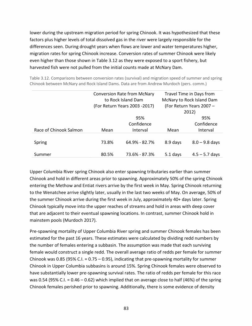
83
lower during the upstream migration period for spring Chinook. It was hypothesized that these
factors plus higher levels of total dissolved gas in the river were largely responsible for the
differences seen. During drought years when flows are lower and water temperatures higher,
migration rates for spring Chinook increase. Conversion rates of summer Chinook were likely
even higher than those shown in Table 3.12 as they were exposed to a sport fishery, but
harvested fish were not pulled from the initial counts made at McNary Dam.
Table 3.12. Comparisons between conversion rates (survival) and migration speed of summer and spring Chinook between McNary and Rock Island Dams. Data are from Andrew Murdoch (pers. comm.)
Race of Chinook Salmon
Conversion Rate from McNary to Rock Island Dam
(For Return Years 2003 -2017)
Travel Time in Days from McNary to Rock Island Dam
(For Return Years 2007 – 2012)
Mean
95% Confidence
Interval
Mean
95% Confidence
Interval
Spring 73.8% 64.9% - 82.7% 8.9 days 8.0 – 9.8 days Summer 80.5% 73.6% - 87.3% 5.1 days 4.5 – 5.7 days
Upper Columbia River spring Chinook also enter spawning tributaries earlier than summer
Chinook and hold in different areas prior to spawning. Approximately 50% of the spring Chinook
entering the Methow and Entiat rivers arrive by the first week in May. Spring Chinook returning
to the Wenatchee arrive slightly later, usually in the last two weeks of May. On average, 50% of
the summer Chinook arrive during the first week in July, approximately 40+ days later. Spring
Chinook typically move into the upper reaches of streams and hold in areas with deep cover
that are adjacent to their eventual spawning locations. In contrast, summer Chinook hold in
mainstem pools (Murdoch 2017).
Pre-spawning mortality of Upper Columbia River spring and summer Chinook females has been
estimated for the past 16 years. These estimates were calculated by dividing redd numbers by
the number of females entering a subbasin. The assumption was made that each surviving
female would construct a single redd. The overall average ratio of redds per female for summer
Chinook was 0.85 (95% C.I. = 0.75 – 0.95), indicating that pre-spawning mortality for summer
Chinook in Upper Columbia subbasins is around 15%. Spring Chinook females were observed to
have substantially lower pre-spawning survival rates. The ratio of redds per female for this race
was 0.54 (95% C.I. = 0.46 – 0.62) which implied that on average close to half (46%) of the spring
Chinook females perished prior to spawning. Additionally, there is some evidence of density

84
dependent mortality in spring Chinook as there was a positive relationship between pre-
spawning mortality and female abundance. Density dependent mortality was not observed in
summer Chinook females (Murdoch 2017).
UCR scientists plan to determine what habitat attributes are needed by spring Chinook while
they hold and mature prior to spawning (Murdoch 2017). For example, do cold water refuges,
baseflows, and water temperatures limit survival, or is survival dependent upon complex in-
river cover, dense riparian vegetation and cut banks, or a combination of all of these or other
factors? Such information could guide future habitat restoration actions and improve pre-
spawning survival rates.
Hatchery programs for both summer and spring Chinook occur in the Upper Columbia to
supplement natural populations or produce fish exclusively for harvest. In supplementation
programs, hatchery adults are allowed to escape into natural spawning areas. Hatchery fish
produced for harvest may also arrive on spawning grounds. Proportions of hatchery origin
spring and summer Chinook adults spawning in nature (pHOS) and proportions of natural origin
adults used as hatchery broodstock (pNOB) in the Wenatchee, Methow, and Okanogan have
been estimated annually from 1989 to 2016.
These two statistics, pHOS and pNOB, are commonly used to calculate a ratio referred to as the
Proportionate Natural Influence or PNI.5 PNI values approximate the degree to which a
population of salmon consisting of both hatchery and natural origin spawners maintains the
original natural population’s genetic properties. The higher the PNI value the greater the
genetic affinity to the natural population. The Hatchery Scientific Review Group, which co-
developed this concept, recommends that PNI values in integrated hatchery programs should
be greater than 0.67. PNI values for spring and summer Chinook were estimated from mean
values provided by Andrew Murdoch (Table 3.13). The advent of selective sport fisheries above
Priest Rapids Dam since 2014 have substantially reduced pHOS values (Murdoch 2017) so
current PNI values are likely greater than those shown in Table 3.12. Nonetheless, past PNI
values suggest that Upper Columbia River spring Chinook populations in the Wenatchee and
5 The general formula for PNI is: pNOB/(pNOB + pHOS). Recently the pHOS term has been modified in recognition
that hatchery fish may not produce as many adult offspring as natural origin adults. This new term is referred to as pHOSeff which equals RRS * pHOScensus. RRS is an estimate of the relative reproductive success of hatchery adults when compared to natural origin counterparts. Suppose that RRS is estimated to be 0.8, in this instance a census pHOS of 50% would be reduced down to 40% resulting in a higher PNI than if the original pHOScensus value had been used. For a detailed explanation of the PNI concept see HSRG (Hatchery Scientific Review Group). 2014. On the Science of Hatcheries: An updated perspective on the role of hatcheries in salmon and steelhead management in the Pacific Northwest. A. Appleby, H.L. Blankenship, D. Campton, K. Currens, T. Evelyn, D. Fast, T. Flagg, J. Gislason, P. Kline, C. Mahnken, B.Missildine, L. Mobrand, G. Nandor, P. Paquet, S. Patterson, L. Seeb, S. Smith, and K. Warheit. June 2014. Available online: hatcheryreform.us

85
Methow were likely exposed to higher levels of potential domestication selection than summer
Chinook.
Table 3.13. Estimated pNOB, pHOS, and PNI values for Upper Columbia River Chinook salmon populations ; mean pNOB and pHOS values (1989 – 2016) were obtained from Andrew Murdoch (pers. comm.).
Upper Columbia River Subbasin
Race of Chinook Salmon
% Natural Origin
Broodstock (pNOB)
% Hatchery Origin Spawners
(pHOS)
Proportionate
Natural Influence
Wenatchee River
Summer 92.4 13.8 0.869
Spring 54.6 45.0 0.548 Methow Summer 74.3 33.1 0.691 Spring 37.0 57.4 0.391 Okanogan Summer 74.3 40.7 0.646
3.3.1.4. Hybridization and Redd Superimposition
In 2006, the USFW began a RME study to measure redd superimposition and hybridization rates
between summer and spring Chinook salmon in the Entiat subbasin. Adult summer and spring
Chinook were found contemporaneously in portions of the Entiat River. Stream surveys were
conducted from August 9 through November 15, and an average of 441 spring and summer
Chinook redds were counted during 2006-2014. Generally, 60 or more were built when both
races were in the river together, suggesting hybridization was possible on ~14% of the Chinook
redds. Male summer Chinook could have been present at 9% (17/197) of the spring Chinook
redds, while spring Chinook males were potentially present at 18% (45/244) of the summer
Chinook redds (Figure 3.26; Desgroseillier et al. 2017). Hybridization was assessed on
approximately 1,000 Chinook juveniles leaving the Entiat River in 2011 and 3.6% (32) were
found to be hybrids. Additional hybrids were discovered rearing in the Entiat during the winter.
To date it has not been possible to determine whether hybrids have returned as adults or
contributed to the recruitment of juveniles. However, an examination of the effects of
hybridization between fall-run Chinook salmon (tule and up-river bright Chinook) in the
Columbia Basin (Smith and Engle 2011) concluded that hybrid juveniles were not viable and
thus likely reduce overall population productivity (Desgroseillier et al. 2017). Whether the same
is true for spring x summer hybrids is not known.

86
Figure 3.26. The spatial distribution of spring and summer Chinook salmon redds in the Entiat subbasin. Overlap of redds occurred in Valley Segments (VS) 2-3. Orange oval indicates area where temporal and spatial overlap occurred. (Image taken directly from Desgroseillier et al. presentation (2017)).
Redd superimposition or the multiple use of a spawning site within a spawning season was also
examined in the Entiat River. Because of differences in maturation timing, summer Chinook
females may excavate nest pockets in locations that were recently used by spring Chinook.
Murdoch (2017) reported that USFW researchers had observed superimposition on ~19% of the
spring Chinook redds they surveyed in the Entiat. The impact that superimposition may have on
egg-to-fry survival can be variable and depends upon a number of factors. For instance,
Chinook eggs are fairly immune to mechanical shock if embryos have accrued 190 temperature
Summer Chinook Redds
Spring Chinook Redds

87
units CO prior to dislodgement or movement (Jensen 2003). Additionally, nest depth is related
to female length and larger females are expected to create deeper nests (Steen and Quinn
1999). Because spring Chinook are generally smaller than summer Chinook, their deposited
eggs may be particularly vulnerable to dislodgement due to the digging activities of larger
summer Chinook. Finally, the majority of eggs deposited by a female are often placed into her
first two nests (de Gaudemar et al. 2000). These will be located at the tail end of a redd and are
often covered by a substantial layer of gravel placed there by the final digging actions of a
female. Typically, newly arriving females are attracted to the anterior portions of pre-existing
redds. This is where the previous occupant has created a depression or “pot” which accelerates
stream flows and accentuates water interchange into the substrate. Knowing when and which
portions of a redd were disturbed would help clarify the potential damage caused by multiple
usage of the same spawning area.
Temporal and spatial overlap information on adult spring and summer Chinook is likely
available for the Wenatchee and Methow subbasins. This information should be used to
determine the degree of overlap that exists between these two races in the above subbasins.
Since spawner density is known to affect distribution patterns (Murdoch 2017), multiple year
assessments should take place. Additionally, analyses on hybridization rates and the occurrence
of redd superimposition similar to those performed in the Entiat are encouraged in the
Wenatchee and Methow subbasins. Such analyses would increase our understanding of the
relative importance of these factors on spring Chinook productivity. Are redd superimposition
or hybridization major factors constraining spring Chinook abundance or do they occur rarely
and are of little demographic importance?
3.3.2. Comparisons between Juvenile Summer and Spring Chinook Salmon
Juvenile trapping operations occur throughout the Upper Columbia Basin and are implemented
to keep track of the abundance and timing of juvenile salmonid migrations. Such data are not
only useful for forecasting future adult abundances but also allow managers and researchers to
potentially detect changes in freshwater productivity, survival, growth, and alterations in
juvenile life histories. Recently, genetic methods have been used to identify the racial origin of
out-migrating juvenile Chinook salmon. These studies revealed that both juvenile spring and
summer Chinook had more diverse out-migration patterns than previously thought.
3.3.2.1. Juvenile Life Histories
In Upper Columbia River subbasins that support both summer and spring Chinook juveniles,
fisheries managers have assumed that subyearling emigrants leaving in the early summer (e.g.,
June and July), are summer Chinook while those emigrating as yearlings in late fall through the
early spring are spring Chinook. Similarly, 0+ spring Chinook smolts were believed to leave

88
beginning in August, peaking as new yearlings in mid- to late October and finishing as 1+
migrants in late December (Desgroseillier et al. 2017). Recent genetic analyses of tissue samples
from juvenile migrants revealed a much more complicated suite of emigration patterns than
expected (Desgroseillier et al. 2017).
Samples collected from mid-September through November revealed the expected upsurge in
spring Chinook juveniles. However, a surprisingly high percentage (~57%) of the subyearlings
leaving the Entiat in July were spring Chinook. This meant that thousands of juveniles that
previously had been assumed to be summer Chinook were actually spring Chinook. Samples
obtained from juveniles rearing in the Entiat during the summer and winter of 2012, 2013, and
2014 indicated that the percentage of each race rearing in different valley segments of the
Entiat remained relatively constant from one year to the next. During the summer sampling
period, a positive correlation between rkm and the proportion of spring Chinook juveniles
rearing in the subbasin was found. This tendency was not seen during the winter sampling
period suggesting that spring Chinook juveniles were moving downstream, most likely seeking
overwintering rearing areas. Surprisingly, a relatively high percentage (~12%) of summer
Chinook overwintered in the Entiat subbasin (Desgroseillier et al. 2017).
The results of the genetic analyses on sampled Chinook juveniles have a number of
management implications that were emphasized by Desgroseillier et al. (2017). First,
undervaluing the number of spring Chinook juveniles produced from the Entiat has inflated SAR
values and simultaneously underestimated egg-to-fry survival and emigrant per redd values.
Incorrect values in these metrics may disguise density dependence, obscure locations in the life
cycle where bottlenecks are occurring, and possibly lead to incorrect productivity or
recruit/spawner ratios and erroneous conclusions about the capacity of the environment to
produce juvenile spring and summer Chinook.
Second, the distribution patterns shown in Table 3.14 led Desgroseillier et al. (2017) to make
two general recommendations about where habitat restoration for Chinook juveniles ought to
be focused. If the goal is to enhance spring Chinook capacity during their first spring and
summer in freshwater, then upper portions of the Entiat should be targeted for restoration
where spring Chinook are concentrated. Conversely, restoration actions designed to provide
overwintering habitat for juvenile Chinook should be distributed throughout the subbasin. This
strategy would also benefit overwintering summer Chinook.

89
Table 3.14. Distribution patterns of summer and spring Chinook salmon juveniles rearing in the Entiat subbasin during the summer (August) and winter (March) as revealed by genetic analyses of 542 samples (405 from the summer period and 137 from the winter period). See Figure 3.26 for locations of valley segments. Percentage data are from Tom Desgroseillier (pers. comm.)
Sampling Area
(Valley
Segment)
Location
(River
Kilometer)
Summer Sampling Period
(August)
Winter Sampling Period
(March)
% Summer
Chinook
% Spring
Chinook
% Summer
Chinook
% Spring
Chinook
VS-1 4.2 47 53 0 100
VS-1 7.4 52 48 0 100
VS-1 10.3 52 48 0 100
VS-1 23.4 8 92 43 57
VS-2 28.1 52 48 29 71
VS-2 31.6 24 76 20 80
VS-3 36.7 12 88 6 94
VS-3 40.2 13 87 8 92
VS-3 42.7 5 95 0 100
VS-3 44.6 5 95 8 92
The abundance of yearling summer Chinook in the Entiat appears to be greater than
abundances in other Upper Columbia subbasins. Genetic assignments of yearling Chinook
rearing in the Wenatchee River over six sampling years (2004 – 2007 and 2012) indicated a
lower level of yearling summer Chinook (mean of 3.2%, range 0.9% - 7.2%). Similarly, a single
year of genetic analyses of overwintering Chinook in the Methow also showed just 1.7% of the
yearlings were summer Chinook (Murdoch 2017). The Entiat is a smaller and less complex
subbasin than the Wenatchee and Methow subbasins, which may explain why a substantial
percentage of spring Chinook emigrate as subyearlings from the Entiat. However, the higher
relative incidence of yearling summer Chinook in the Entiat remains to be explained. It appears
that the upper portions of valley segment 1 (VS-1) and valley segment 2 (VS-2) are favored by
this race as overwintering locations (Table 3.14). A careful inventory of habitat attributes in this
portion of the Entiat might provide information about overwintering habitat and discern if the

90
high percentage of summer Chinook in this portion of the river simply is due to a paucity of
juvenile spring Chinook at these locations.
Rotary screw trap (RST) data from the Upper Columbia subbasins indicated that a substantial
portion of Chinook juveniles exit their natal streams as subyearlings in late June and July. This
exodus of subyearling Chinook prompted Desgroseillier et al. (2017) to investigate where both
spring and summer subyearlings went after they left the Entiat subbasin. PIT tag detections at
tributary arrays and at mainstem dams on the Columbia were used to help decipher the
migratory and rearing strategies used by parr from the two races of Chinook. Additionally, the
residency and migratory patterns exhibited by Entiat spring chinook parr were compared to
those exhibited by spring Chinook parr originating from the Chiwawa (Wenatchee subbasin),
Chewuch, and Twisp rivers (both in the Methow subbasin). This evaluation was conducted to
see if subbasin origin affected parr migratory behavior. The migratory patterns of yearling
smolts produced by both races were also tracked and compared.
Juvenile trapping data showed that large numbers of subyearling Chinook out-migrate as fry (<
50 mm FL) for weeks to months from the Entiat and the Wenatchee subbasins (Murdoch 2017;
Desgroseillier et al. 2017). No assessments have been made on the percentage of the fry that
are of summer or spring origin. Additionally, little is known about fry behavior and survival once
they enter mainstem reservoirs. More is known about parr (> 50 mm) who continuously out-
migrate throughout summer and fall months. Desgroseillier et al. (2017) found that spring
Chinook subyearlings from the Entiat migrated downstream and overwintered in mainstem
reservoirs. None were observed directly migrating to the estuary as subyearlings. Conversely
subyearling summer Chinook parr that emigrated in mid-July through early September often
migrated directly downstream to the estuary. Summer Chinook that emigrated from the Entiat
later in the fall also migrated downstream but often overwintered in mainstem reservoirs prior
to entering the estuary during the following spring.
The general tendency of Entiat subyearling spring Chinook to enter the estuary as yearlings was
similar to the life history patterns of spring Chinook in the Twisp, Chiwawa, and Chewuch
subbasins. PIT tag detections on these fish showed that a large portion moved downstream
<150 rkm before overwintering. Unlike the Entiat fish, however, almost none of the Methow or
Wenatchee subyearlings left their natal streams prior to overwintering in downstream reaches
in the subbasins (Desgroseillier et al. 2017)
Fish that stayed in their natal subbasins and emigrated as yearlings entered the mainstem from
early February through the end of May. Spill to facilitate juvenile emigration in the mainstem
begins in mid-April and by that time almost 60% of the yearling Chinook smolts (largely spring
Chinook smolts) have already entered the mainstem. Conversely, less than 10% of summer
Chinook subyearlings have entered the mainstem before the onset of spill. Thus, the later

91
migration timing of summer subyearlings matches well with the increased spill regime
(Murdoch 2017) and they are expected to have lower mortality rates due to dam passage.
The life history patterns revealed by RST trapping and PIT Tag detections showed that the life
history patterns of both summer and spring Chinook juveniles in the Upper Columbia are more
complex than originally thought. Assumed and observed life history patterns of Entiat spring
and summer Chinook are compared in Table 3.15. This table and data from the Murdoch (2017)
and Desgroseillier et al. (2017) indicate that:
Summer Chinook have greater juvenile life history diversity than spring Chinook and
therefore may have greater intrinsic resilience than spring Chinook
Summer Chinook enter the estuary as subyearlings and yearlings over a much broader
span of time than spring Chinook
Later out-migration timing of summer Chinook subyearlings coincides with the
increased spill regime that was established to reduce dam related mortalities. Their
outmigration timing is also better synchronized with increased flows and higher
turbidity due to the spring run-off.
Smaller size at emigration may make summer Chinook less vulnerable to bird predation
if birds prefer larger prey (e.g., Caspian Terns)
Summer Chinook typically rear for shorter periods in tributaries than spring Chinook and
are less likely to experience capacity limitations or survival bottlenecks in subbasins
Contrary to previous thought, some Upper Columbia spring Chinook juveniles rear in
mainstem reservoirs for prolonged periods
The lower 235 rkm between Bonneville Dam and the ocean was identified as a feeding
area for juvenile salmonids where competition for resources with other species and age
classes may occur

92
Table 3.15. Comparisons between assumed and observed life history patterns in Upper Columbia River summer and spring Chinook juveniles. Newly acquired data indicate unexpected mainstem use by spring Chinook and tributary rearing and overwintering by summer Chinook. Table modified from Desgroseillier et al. (2017).
CLASSIC LIFE HISTORY (ASSUMED) OF ENTIAT CHINOOK SALMON
RACE LOCATION
Season
FALL WIN SPR SUM FALL WIN SPR
Summer
Gravel X X
Emergence X
Tributary X X X
Columbia R. X X
Estuary X X
Ocean X X
Spring
Gravel O O
Emergence O
Tributary O O O O O
Columbia R. O
Estuary O
Ocean O
OBSERVED LIFE HISTORY OF ENTIAT CHINOOK SALMON
RACE LOCATION
Season
FALL WIN SPR SUM FALL WIN SPR
Summer
Gravel X X
Emergence X
Tributary X X X X X
Columbia R. X X X X X
Estuary X X X X
Ocean X X X X
Spring
Gravel O O
Emergence O
Tributary O O O O O
Columbia R. O O O O O
Estuary O
Ocean O
Studies demonstrate that mainstem reservoirs and the lower reach of the Columbia provide
important rearing and overwintering areas for Upper Columbia River Chinook (e.g.,

93
Desgroseillier et al. 2017) and illustrate the need for additional mainstem research. Some
studies have assessed the effects of channel catfish, smallmouth bass, and walleye predation on
juvenile salmonids, but holistic, regional multi-species studies are needed to understand
cumulative effects (Sanderson et al. 2009). Additionally, possible effects of competition
between juvenile salmonids and American Shad for planktonic food in the lower river and
estuary is yet to be determined.
3.3.2.2. Juvenile Life History Strategies and the Production of Adults
Both Murdoch (2017) and Desgroseillier et al. (2017) examined the juvenile life history
strategies employed by adult salmon returning to Columbia River subbasins. Desgroseillier et al.
(2017) compared adult return rates (SARs) among three types of juveniles returning to the
Entiat; (1) yearlings, (2) subyearlings that emigrated from the Entiat in June – September, and
(3) subyearlings that left during the October-November out-migration period. They also
compiled data on Entiat adults that were grouped by rearing area; (1) yearlings that stayed in
the Entiat, (2) reservoir yearlings, and (3) subyearlings that immigrated directly to the ocean.
Out of the two yearling strategies employed, those that resided in mainstem reservoirs had
higher SAR values than yearlings that had remained in the Entiat prior to out-migration.
Additionally, juveniles that emigrated from the Entiat and entered the estuary as subyearlings
(summer Chinook) also had higher SAR values than yearling fish staying in the Entiat. Juveniles
that reared in reservoirs and out-migrated as yearlings had the highest SAR values (Table 3.16).
At present the factors responsible for these patterns in SAR values are not entirely understood.
Table 3.16. Smolt-to-adult return rates (SARs) in Chinook salmon returning to the Entiat that adopted different life histories (yearling and subyearling) and juvenile rearing areas (natal stream, reservoir, and ocean) by brood year. Data from Tom Desgroseillier (pers. comm.)
Brood Year
SARs in Yearling and Subyearlings Rearing Area Effects on SARs Yearling
Sub Yearling (Jun – Sep)
Sub Yearling (Oct –Nov)
Natal Stream Yearling
Reservoir Yearling
Ocean Type Subyearling
2006 0.80% 0.12% 0.56% 0.80% 2.99% N/A 2007 1.34% N/A 0.17% 1.34% 3.64% N/A 2008 0.90% N/A 0.20% 0.90% N/A N/A 2009 0.28% 0.11% 0.20% 0.28% 0.75% 0.51% 2010 0.82% 0.17% 0.26% 0.82% 2.81% 1.18% 2011 1.08% 0.36% 0.39% 1.08% 1.20% 2.25%
Murdoch (2017) examined the effect of juvenile life history on adult production with a different
approach. He documented the percentage of adults that had utilized a yearling, reservoir

94
yearling, and subyearling juvenile strategy on a return year basis. This was estimated for adult
Chinook returning to the Wenatchee, Methow, and Okanogan Rivers for return years 1993 –
2015. Percentage values from Andrew Murdoch (pers. comm.) were used in Kendall’s Tau
correlations to see if the proportion of adults using the subyearling, reservoir, and yearling
strategies were similar in each subbasin for each return year. The proportion of adults using
each strategy in each return year was remarkably similar among the three subbasins (Table
3.17). Additionally, a substantial increase in the subyearling strategy was observed along with a
corresponding decrease in the yearling and reservoir yearling strategies in adult Chinook from
the early 1990s to the present. Representative scatter plots illustrate these trends in Figure
3.27.
Table 3.17. Results of Kendall’s Tau correlations conducted on the percentages of adults possessing different juvenile life histories that returned in the same year but to different Upper Columbia subbasins (performed to see if adults returning in the same year but to different subbasins used similar juvenile life histories). Percentage data obtained from Murdoch presentation (2017).
Subbasins
Correlation
Juvenile Life History Type
Subyearling Reservoir Rearing
Yearling
Tau
p Value
Tau
p Value
Tau
p Value
Wenatchee & Methow
% of adults in the Wenatchee vs. % of adults in the Methow with the same
juvenile life history 0.836 <.01 0.737 <.01 0.605 <.01
Wenatchee & Okanogan
% of adults in the Wenatchee vs. % of adults in the Okanogan with the same
juvenile life history 0.787 <.01 0.649 <.01 0.512 <.01
Methow & Okanogan
% of adults in the Methow vs. % of adults in the Okanogan with the same
juvenile life history 0.810 <.01 0.735 <.01 0.728 <.01

95
Figure 3.27. Percentage of natural origin adults returning in the same year to the Wenatchee and Methow subbasins that utilized the juvenile subyearling (A) and reservoir (B) strategies and percentage of Wenatchee (black circles) and Methow (red circles) of naturally produced adults that used the subyearling (C) and yearling (D) life histories by return year. Data from Murdoch (2017).
The marked increase in the subyearling strategy and corresponding decrease of the yearling
strategy in all three subbasins might be due to conditions in the subbasins or conditions they
encountered in the mainstem after leaving their natal subbasins. Exploring how environmental
and biological variables (e.g., flow, water temperature, water travel time, predator abundance,
habitat attributes) influence the survival of fish using these different life history strategies may
help identify population bottlenecks and guide future restoration actions.
3.4. Pinniped Predation
3.4.1. Background Information
The Upper Columbia Salmon Recovery Board (UCSRB) Recovery Plan (Final 9-13-2007) identifies
pinnipeds, including harbor seals (Phoca vitulina), California sea lions (Zalophus californianus),
and Stellar sea lions (Eumetopia jubatus), as the primary marine mammals preying on Chinook
and steelhead originating from the Upper Columbia Basin. As part of the Recovery plan, “the
UCSRB supports immediate adoption of more effective predator control programs, including
lethal removal when necessary, of the marine and avian predators that have the most
significant negative impacts on returns of Upper Columbia Basin ESA-listed salmonid fish
stocks.”
96
The 2016 five-year Upper Columbia status report provides an updated review of information on
pinniped predation and predatory pinniped management (through 2015), including the
following conclusions and recommendations:
“The effect of marine mammal predation on the productivity and abundance of
Columbia River basin salmon and steelhead stocks has not been quantitatively
assessed at this time. The absolute number of animals preying upon salmon and
steelhead throughout the lower Columbia River and Willamette River is not
known. The information available since the last status review clearly indicates
that predation by pinnipeds on listed stocks of Columbia River basin salmon
[including Upper Columbia spring Chinook] and steelhead, as well as eulachon,
has increased at an unprecedented rate. So while there are management efforts
to reduce pinniped predation in the vicinity of Bonneville Dam, this management
effort is insufficient to reduce the severity of the threat, especially pinniped
predation in the Columbia River estuary (river miles 1 to 145), and at Willamette
Falls. Recommendations: (1) expand pinniped monitoring efforts to assess
predator-prey interactions between pinnipeds and listed species, (2) maintain
predatory pinniped management actions at Bonneville Dam to reduce the loss of
up- river listed salmon and steelhead stocks, (3) complete life-cycle/extinction
risk modeling to quantify predation rates by predatory pinnipeds on listed
salmon and steelhead stocks in the Columbia River and Willamette River, and (4)
expand research efforts in the Columbia River estuary on survival and run timing
for adult salmonids migrating through the lower Columbia River to Bonneville
Dam.”
3.4.2. ISAB’s Past Findings, Conclusions, and Recommendations
Most of the theoretical and existing evidence available to the ISAB to answer pinniped
predation questions in the current review has been thoroughly reviewed in past ISAB reports on
food webs (ISAB 2011-1), density dependence (ISAB 2015-1), critical uncertainties (ISAB/ISRP
2016-1), predation metrics (ISAB 2016-1), and Interior Columbia Basin life-cycle models (ISAB
2013-5, ISAB 2017-1). Therefore, we briefly summarize ISAB’s relevant past findings,
conclusions, and recommendations.
The ISAB’s Food Web Report (ISAB 2011-1) included a review of information through 2010 on
the increasing abundance of pinniped predators and predation by sea lions at Bonneville Dam.
The ISAB concluded that an important knowledge gap is the lack of data on rates of predation
by apex predators (birds, fish, marine mammals) on the region’s fish (salmon, steelhead,
lamprey, sturgeon, eulachon, etc.) resources. These data are needed to better understand food
web dynamics and total ecosystem productivity in the Columbia River Basin. The ISAB
recommended: (1) using models to estimate system-scale consequences of increases or
decreases in predation rates, (2) quantifying predator abundance in space and time and using

97
bioenergetic and community process models to estimate system-scale consequences, and (3)
determining the effects of predation on salmonids by piscivorous fish, seabirds, and mammals
and whether these effects are additive or compensatory; doing this by comparing predation
rates as a percent of the juveniles passing Bonneville Dam or PIT tag detectors in the lower
estuary with appropriate smolt-to-adult survival estimates (SARs) for different ESUs and run
timings.
The ISAB’s Density Dependence Report (ISAB 2015-1) reviewed evidence of predation effects on
density dependence of salmon populations in the Upper Columbia and Snake river basins, and
identified the lack of information about predation on adult salmon by pinnipeds (seals and sea
lions) as a primary data gap. The ISAB considered predation on adult salmon during upstream
migration to be of particular concern because it may reduce the potential spawning population
more than an equivalent rate of predation at earlier life stages. By the time adult salmon enter
the Columbia River estuary, they have already survived numerous threats in both freshwater
and marine environments, and all are potentially valuable for harvest or spawning. Evidence
reviewed by the ISAB showed that the escapement goal for spring Chinook counted at
Bonneville Dam (115,000 fish) had been met or exceeded since 2008 despite evidence that
predation of salmon by pinnipeds is increasing. Moreover, there is evidence for density
dependence over the entire life cycle for most interior populations of spring and summer
Chinook salmon (24 out of 26 populations remained strongly compensatory; Zabel and Cooney
2013), even though depensatory mortality6 likely occurs at some life stages. However, among
Upper Columbia spring Chinook populations evaluated (Entiat, Methow, and Wenatchee), only
the Wenatchee population did not exhibit a significant density-dependent relationship (Zabel
and Cooney 2013).
Surprising new evidence indicated a steady decline in estuarine survival of the combined runs
of adult middle and Upper Columbia River spring Chinook and Snake River spring/summer
Chinook (from 90% in 2010 to 69% in 2013) (Wargo Rub et al. 2014). Survival was consistently
higher for Chinook arriving late in the run compared to those returning early or at the peak,
when predation by pinnipeds would have been more intense (Wargo Rub et al. 2014). The
declining survival rates also coincided with the growing presence of sea lions and seals in the
estuary. The number of sea lions identified at haul out sites near Astoria in 2013 was five times
that observed during each of the previous three years, and a still larger number was observed
in 2014 (Wargo Rub et al. 2014). The ISAB concluded that there were no reliable estimates of
total pinniped abundances in the Columbia River estuary, integrated over all seasons, and the
impacts of pinniped predation on salmonids in the Columbia River were still unknown or largely
speculative. For example, in theory, even if pinniped predation on interior populations of
6 Mortality caused by individual predators is typically depensatory, which means that the impact on a salmon prey population from individual pinniped predators is highest when fewer prey are present and decreases when more salmon prey are available because predators become satiated and reduce their feeding rate. This typical functional response can be offset by an increase in the number of predators due to aggregation in the short term or increased predator reproduction and abundance in the long term.

98
spring/summer Chinook was reduced, salmon productivity (recruits per spawner) would not
increase because escapement goals (at Bonneville) were met and most populations exhibited
density dependence. Because depensatory mortality may pose a threat to ESA-listed
populations, the ISAB recommended further quantification of mortality and evaluation of life-
cycle recruitment in salmon populations targeted by pinnipeds. Further studies were needed to
track pinniped abundance in the estuary, and to confirm that salmon mortality attributed to
pinnipeds is depensatory, as expected, and as suggested by studies to date.
The ISAB’s Critical Uncertainties Report (ISAB/ISRP 2016-1) identified predation as a new critical
uncertainty for the Council’s Fish and Wildlife Program and two critical questions for this
uncertainty: (1) To what extent is the viability or abundance of native fish and wildlife
populations in the Columbia River Basin jeopardized by predation? and (2) How effectively can
undesirable impacts of predation be ameliorated by management actions including
hydrosystem operations, habitat modifications, and predator population control? These critical
questions were included in the Council’s 2017 Research Plan.
The ISAB’s Predation Metrics Report (ISAB 2016-1) reviewed and recommended potential
alternative metrics for evaluating and comparing the effects of predation at different stages in
the life cycle of anadromous salmon and steelhead in the Columbia River Basin. The ISAB
considered compensatory mortality to be the most important uncertainty to address when
developing a predation metric. The ISAB reviewed evidence for mechanisms of compensation,
including (1) density dependent survival due to factors other than predation, (2) selective
predation based on fish size and condition, and (3) switching behavior of predators, which may
be caused by a change in abundances of alternative prey species or when secondary predators
increase predation on salmon following control of the primary predator. Considerable
compensation in predation-related mortality may occur between juvenile and adult life stages,
but additional compensation may also occur during the subsequent spawner-to-smolt stage,
indicating the need to consider predation within the context of the entire life cycle.
A review and comparison of three alternative metrics using a standard set of evaluation criteria
revealed that a single metric would not be adequate for evaluating all goals. The ISAB
recommended: (1) using and further refining two types of metrics currently in use in the Basin,
that is, Equivalence-factor metrics (for example, adult equivalents), which can be used to
compare the effects of predation on salmon and steelhead at different points in their life cycle,
and a population growth rate metric (also called delta-lambda, Δλ), which can be used to
compare how different predation scenarios affect rates of population recovery or decline; (2)
adjusting the equivalence-factor metrics and the population growth rate metric (Δλ) to account
for assumed or estimated compensation in mortality, and (3) placing predation mortality in the
context of a life-cycle model that can be used to evaluate multiple factors affecting salmon
survival and interactions among those factors in modeled scenarios and verified with data. This
approach could help guide research, monitoring, and evaluation of predation throughout the
99
salmonid life cycle, both to provide the data necessary to parameterize and verify models, and
to refine metrics.
The ISAB’s Life Cycle Modeling Report (ISAB 2017-1) reviewed NOAA’s 2017 report on Interior
Columbia Basin Life Cycle Modeling, and builds on a previous ISAB review in 2013 (ISAB 2013-5).
In Chapter 6.a of the NOAA report (Population-specific pinniped predation; Sorel et al. 2017),
modelers used tag-recapture data to estimate population-specific survivals of adult spring-
summer Chinook salmon migrating from the mouth of the Columbia River to Bonneville Dam.
The modeling results indicated a decline in Chinook salmon survival as pinniped density
increased. Early-migrating spring Chinook salmon populations that entered the lower river in
late winter or early spring had a higher risk of mortality from pinniped predation than later
migrating populations. Compared to a baseline period (1998-2012), apparent survival of adult
Upper Columbia spring Chinook in 2013-2015 decreased substantially, i.e., average survival was
22% lower than survival during the baseline period for the earliest-arriving population
(Methow) and 11% lower for intermediate-arriving populations (Entiat and Wenatchee).
Investigators speculated that a 22% decrease in survival would significantly affect population
viability if sustained.
The ISAB’s review concluded that treatment and communication of assumptions and
uncertainties in the analysis were not fully addressed by the authors. For example, salmon
mortality due to handling and tagging is presumed to be equal in all years, without discussion of
how variable mortality might affect estimates. Small sample sizes necessitated simplifying
assumptions like constant year effects across populations and constant variances within
populations across years, but discussion was limited on robustness to violation of these
assumptions. Uncertainty remains as to whether other causal factors or estimation error—for
example, disease, permanent straying below Bonneville of upriver fish, underestimation of
harvest, artifact of learned behavior by predators (Wargo-Rub et al. 2014)— may be involved in
the apparent decline in survival of adult Upper Columbia spring Chinook from the river mouth
to Bonneville Dam. The ISAB’s recommendations for some specific areas of future research and
implementation of results in life-cycle models included: (1) apply the results of Sorel et al.
(2017) to existing life-cycle models, as recommended by Sorel et al. (2017) and ISAB 2016-1
(Predation Metrics Report) and evaluate the risk of extinction caused by pinniped predation
and tradeoffs between fishing mortality and this predation mortality and the risk of extinction;
(2) extend the model to include parameters for marine mammal predation on adult salmon in
the Columbia River Plume. Explore spatial variation in predation pressure in the plume and
lower river. (3) investigate relationships of fishing and marine mammal predation on adult
salmon; (4) investigate relationships of forage fish density and marine mammal predation on
adult salmon survival; and (5) develop methods to investigate marine mammal predation on
the juvenile freshwater/estuary/early ocean life stages.
A preliminary life-cycle model for Upper Columbia spring Chinook in the Wenatchee subbasin,
reviewed by ISAB in 2013 (ISAB 2013-5), was updated (Jorgensen et al. 2017). Two pinniped

100
predation scenarios of adult salmon survival were modeled, and results indicated the biggest
increase in spawner abundance occurred when estuarine adult survival increased to historical
levels, as might result from reduced pinniped predation, and when the hatchery programs
resumed operations to current levels. The ISAB’s review (ISAB 2017-1) concluded:
“Given the many assumptions and fixed parameter values, the [model] outputs
should be used in a qualitative fashion only, e.g., to rank actions in terms of
effectiveness. It would be difficult to assign a quantitative gain to any of the
scenarios that were performed.”
“Similarly, it will be difficult to use the model in its current stage of development
for adaptive management, because it will be unknown whether a failure to see a
predicted response to a management action in the real world is due to stochastic
variability or to inadequacy of the life-cycle model.”
3.4.3. Conclusions about Pinniped Predation
Are pinnipeds potentially a significant source of mortality for Upper Columbia spring Chinook?
The best available scientific evidence, as reviewed by ISAB in past reports (see above, ISAB’s
Past Findings, Conclusions, and Recommendations) and in new (2017) reports and publications,
indicates that pinnipeds are potentially a significant source of mortality for Upper Columbia
spring Chinook adults. However, population-specific estimates of predation impacts on Upper
Columbia spring Chinook were not available to the ISAB at the time of this review. The
estimated consumption of combined populations of Chinook salmon by pinnipeds in the
Columbia River increased sharply over the past decade, likely exceeding removals by fisheries
(Chasco et al. 2017) (Figure 3.28). Potential impacts varied by pinniped species and salmon life
stage. For example, in 2015 estimated biomass (metric tonnes, t) and numbers of Chinook
salmon consumed in the Columbia River estuary varied among harbor seals (14 t, including
1000 adults and 312,000 smolts), California sea lions (219 t, including 46,000 adults), and Steller
sea lions (227 t, including 47,000 adults) (Chasco et al. 2017). In 2017, the reduced salmonid
runs and persistently high numbers of pinnipeds in the latter part of the season suggests that
the total impact by pinnipeds on the year’s salmonid run may be large (Tidwell et al. 2017)
(Figure 3.29).

101
Figure 3.28. Estimates of consumption of Chinook salmon by pinniped predators in the Columbia River, with uncertainty, in terms of the biomass (primary axis) and number (secondary axis) of Chinook salmon consumed, 1975-2015. Source: Figure 7, Chasco et al. (2017).
Figure 3.29. Preliminary estimated pinniped predation at Bonneville Dam in 2017, compared to the 10-yr average (Tidwell et al. 2017). Between 13 May and 2 June 2017 an estimated 1837 ± 130 adult salmonids were consumed (10-yr average estimate of 494 adult salmonids for the same time period). From 1 January to 2 June 2017, an estimated, but not adjusted, 4993 ± 234 adult salmonids (82% spring Chinook) were consumed by pinnipeds. The combined runs were delayed relative to previous years and smaller than the long-term average. As such, the duration of pinniped presence and levels of fish predation were protracted relative to the 10-year average. The reduced salmonid runs and persistently high numbers of pinnipeds in the latter part of the season suggests that the total impact by pinnipeds on 2017’s salmonid run may be large.
The Chasco et al. (2017) estimates of in-river consumption of adult (ocean age two and greater)
Chinook salmon by sea lions in the Columbia River from January to August in 2015 was 65,000
(49,000–81,000), were lower than the most recent direct, tagging-based estimate of 95,000
(61,000–127,000) spring/summer Chinook (Michelle Rub, pers. comm., August 7, 2017, as cited
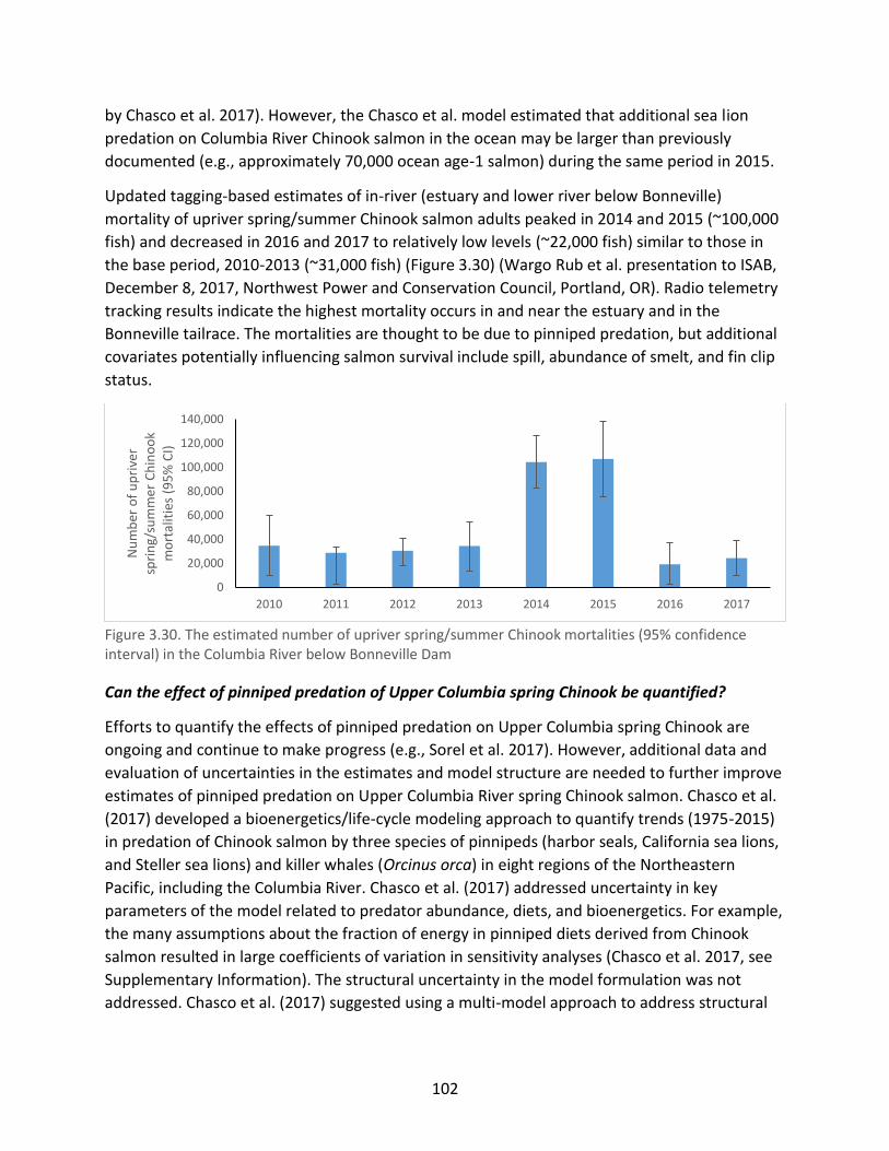
102
by Chasco et al. 2017). However, the Chasco et al. model estimated that additional sea lion
predation on Columbia River Chinook salmon in the ocean may be larger than previously
documented (e.g., approximately 70,000 ocean age-1 salmon) during the same period in 2015.
Updated tagging-based estimates of in-river (estuary and lower river below Bonneville)
mortality of upriver spring/summer Chinook salmon adults peaked in 2014 and 2015 (~100,000
fish) and decreased in 2016 and 2017 to relatively low levels (~22,000 fish) similar to those in
the base period, 2010-2013 (~31,000 fish) (Figure 3.30) (Wargo Rub et al. presentation to ISAB,
December 8, 2017, Northwest Power and Conservation Council, Portland, OR). Radio telemetry
tracking results indicate the highest mortality occurs in and near the estuary and in the
Bonneville tailrace. The mortalities are thought to be due to pinniped predation, but additional
covariates potentially influencing salmon survival include spill, abundance of smelt, and fin clip
status.
Figure 3.30. The estimated number of upriver spring/summer Chinook mortalities (95% confidence interval) in the Columbia River below Bonneville Dam
Can the effect of pinniped predation of Upper Columbia spring Chinook be quantified?
Efforts to quantify the effects of pinniped predation on Upper Columbia spring Chinook are
ongoing and continue to make progress (e.g., Sorel et al. 2017). However, additional data and
evaluation of uncertainties in the estimates and model structure are needed to further improve
estimates of pinniped predation on Upper Columbia River spring Chinook salmon. Chasco et al.
(2017) developed a bioenergetics/life-cycle modeling approach to quantify trends (1975-2015)
in predation of Chinook salmon by three species of pinnipeds (harbor seals, California sea lions,
and Steller sea lions) and killer whales (Orcinus orca) in eight regions of the Northeastern
Pacific, including the Columbia River. Chasco et al. (2017) addressed uncertainty in key
parameters of the model related to predator abundance, diets, and bioenergetics. For example,
the many assumptions about the fraction of energy in pinniped diets derived from Chinook
salmon resulted in large coefficients of variation in sensitivity analyses (Chasco et al. 2017, see
Supplementary Information). The structural uncertainty in the model formulation was not
addressed. Chasco et al. (2017) suggested using a multi-model approach to address structural
0
20,000
40,000
60,000
80,000
100,000
120,000
140,000
2010 2011 2012 2013 2014 2015 2016 2017
Nu
mb
er o
f u
pri
ver
spri
ng/
sum
mer
Ch
ino
ok
mo
rtal
itie
s (9
5%
CI)

103
uncertainty, e.g., by comparing their bioenergetics approach to other methods such as
individual-based models or time series modeling.
3.5. Recommendations
Identifying limiting factors
The ISAB recommends integrating the results of the different approaches—limiting factors
analysis, density dependence analysis, and life-cycle modeling—for identifying limiting factors
to guide future revision of the Biological Strategy of the RTT and the Recovery Plan for spring
Chinook salmon. This integration will require a collaborative process that includes significant
participation by experts, practitioners, and management teams from all Hs. To date, analysis
has focused on limiting factors related to habitat conditions. The limitations of four Hs on spring
Chinook populations are considered in isolation.
We recommend the UCSRB, RTT, and co-managers to consider an effort to synthesize the
results of the different approaches for identifying limiting factors to guide future revision of the
Biological Strategy of the RTT and the coordination of actions for spring Chinook salmon by the
UCSRB.
If return of adult spawners or recruitment substantially limit recovery in the Upper Columbia,
then discussions of the effects of harvest on escapement between co-managers and
participants in the UCSRB could strengthen future approaches to improve recovery efforts.
Integration of Biophysical and Economic Evaluation of Recovery Actions
Biophysical limitations on spring Chinook are considered in limiting factors analysis, density
dependence analysis, and life-cycle modeling. Economic analysis—relaxing which constraint can
most cost-effectively improve abundance in the shortest period of time—has rarely has been
used to measure the operational importance of different limiting factors. We recommend the
development of integrated analyses in which biophysical analyses of limiting factors and
economic analysis of the costs associated with different management actions to better inform
recovery actions for UCR spring Chinook salmon. Such analyses would provide quantitative
estimates of the relative cost-effectiveness of alternative recovery actions
Snake River and Upper Columbia River spring Chinook salmon
The ISAB recommends continued comparison of Chinook recovery in both ESUs to determine
which restoration actions are most effective. Rigorous RME programs are essential to
understand the trends and factors that influence them in these two basins. The lower number
of populations and total abundances of the Upper Columbia River spring Chinook ESU
potentially expose them to greater threats than the Snake River spring/summer Chinook ESU.
104
Spring and summer Chinook in the Upper Columbia River
The ISAB recommends continued investigations of the effects of summer Chinook on spring
Chinook in Upper Columbia River subbasins, including effects of hatchery practices, redd
superimposition, competition, outmigration behavior, relative rates of survival and behavior in
the mainstem Columbia, and the relative effects of pinnipeds and harvest in the lower river and
estuary. Summer Chinook may affect the recovery of spring Chinook through competition, redd
superimposition, and introgression. In addition, differences in life histories, habitat
relationships, survival, population demographics, and responses to potential limiting factors by
summer Chinook may reveal critical factors for the recovery of spring Chinook salmon in the
Upper Columbia River.
Analysis of natural origin return numbers for spring and summer Chinook provide a general
demographic overview of how population abundance varies over time. However, grouping
returns by brood year provides a number of important advantages. Juveniles are counted by
cohort or year class, and adults should be counted on a similar basis in demographic analyses.
Foremost among those is the development of recruitment curves that can determine intrinsic
productivity and the population carrying capacity in existing habitat (ISAB 2015-1). Additionally,
smolt-to-recruit (SARs) estimates for each brood year can be made. SAR values could be used to
directly test the effects of the summer spill program on survival and also allow a more refined
assessment of how summer and spring Chinook abundance may be related. Advantages of
using brood year returns as opposed to annual returns have led us to make several suggestions
the researchers may wish to undertake if they are not already underway:7
Add harvest values (by age) to the return numbers for years 1989 – 2016
Evaluate trends of abundance by brood year rather than by return year.
o Anadromous spring Chinook reach maturation at ages 3, 4, and 5. Summer
Chinook also mature at these ages and a few may return at age 6. If age data are
available, it will be possible to examine the abundance of fish returning from the
1986 brood year up to the 2010 brood year. This would create a dataset with 25
brood years as opposed to the existing one with 28 return years.
7 Our request to compare the survival and life history strategies of spring and summer Chinook returning to upper Columbia subbasins occurred after our site visit to the upper Columbia. We appreciate the effort undertaken to carry out this unexpected and new assignment. The scientists performing this work indicated that additional comparisons will be made in the future. It is likely that yearly return data will be deconstructed and assembled into brood year survival and abundance data. The suggestions for future analyses were made to affirm the importance of producing and analyzing brood year information.

105
Use return data to populate brood year returns by subbasin rather than aggregating
them into a single number for each race of Chinook salmon. Summer and spring Chinook
returning to the Wenatchee River pass over two fewer dams than those returning to the
Methow and Okanogan River and therefore may be affected by different stressors.
Temporal and spatial overlap information on adult spring and summer Chinook is likely
available for the Wenatchee and Methow subbasins. This information should be used to
determine the degree of overlap that exists between these two races in the above
subbasins. Since spawner density is known to affect distribution patterns (Murdoch
2017) multiple year assessments should take place. Additionally, analyses on
hybridization rates and the occurrence of redd superimposition similar to those
performed in the Entiat are encouraged. They would help determine the relative
importance of these factors on spring Chinook productivity. Are they major factors
constraining spring Chinook abundance or occur rarely and are of little demographic
importance?
Pinniped predation
The ISAB reiterates its recommendations from past reviews (see 3.4.2) and recommends
proceeding with pinniped recommendations in the 2016 five-year Upper Columbia status
report:
“(1) expand pinniped monitoring efforts to assess predator-prey interactions
between pinnipeds and listed species, (2) maintain predatory pinniped
management actions at Bonneville Dam to reduce the loss of up- river listed
salmon and steelhead stocks, (3) complete life-cycle/extinction risk modeling to
quantify predation rates by predatory pinnipeds on listed salmon and steelhead
stocks in the Columbia River and Willamette River, and (4) expand research
efforts in the Columbia River estuary on survival and run timing for adult
salmonids migrating through the lower Columbia River to Bonneville Dam.”
The ISAB considers the second recommendation a necessary precautionary measure while
better data are collected.
The ISAB recommends identifying and investigating other potentially significant sources of
mortality of Upper Columbia spring Chinook smolts and adults in the Columbia River
plume/ocean shelf habitats, estuary, and lower mainstem and tributaries. New information
from NOAA’s tagging and modeling efforts revealed important data gaps, including lack of
population-specific survival estimates for Upper Columbia spring Chinook.
The ISAB recommends use of a variety of approaches to quantify pinniped predation impacts,
such as the ongoing tagging studies and coast-wide bioenergetics/life-cycle modeling. New
information from NOAA’s tagging and modeling efforts revealed some important data gaps,

106
including the lack of population-specific estimates for UCR spring Chinook salmon. To evaluate
assumptions and reduce uncertainties in estimates, modeling efforts would benefit from better
information on the abundance and spatial-temporal distribution of pinnipeds, particularly in the
lower river and estuary, pinniped body mass and digestion efficiencies, and the fraction of
Chinook salmon prey in pinniped diets, as well as better estimates of natural-origin smolt
production, smolt and adult spatial distribution and residence time, size-at age and growth, and
energy density of UC spring Chinook. Comparison of multiple models could reduce structural
uncertainty (e.g., comparing a bioenergetics approach to individual-based models or time series
models).

107
4. Prioritization and Effectiveness of Habitat Restoration and Enhancement
Many habitat protection, restoration, and enhancement projects have been planned and
completed in the Upper Columbia River region since spring Chinook salmon were listed as an
endangered species in 1999. In large part, this is because restoration of tributary habitat is
considered a key requirement for recovery of this salmon stock and one of the most feasible
actions possible to mitigate for degradation of the hydrosystem by dams, native and nonnative
predators, and poor and changing ocean conditions, among other stressors. Toward that end, a
total of $74 million dollars from all funding sources was been spent between 1996 to 2012 to
plan and carry out these habitat projects (UCSRB 2014b).
The effects of habitat restoration interact with those of actions to address the other three Hs—
Hatchery, Hydropower, and Harvest—making it difficult to separate their effects and determine
which actions provide optimum benefits. As a result, biologists and managers have focused on
smolts produced from UCR subbasins as one measure of the effectiveness of habitat projects,
because it is relatively free from influence by other mitigation actions, except for introduction
of hatchery fish (UCSRB 2007). A key measure of smolt productivity is smolts per redd,
determined by dividing smolt output measured using screw traps by redd abundance measured
using field surveys or estimated from counts of adults. Another measure is parr-to-smolt
survival, measured by detections of PIT-tagged fish at PIT-tag antennas in lower river locations
Questions submitted to ISAB:
Are habitat recovery actions being prioritized and sequenced
strategically, given existing knowledge and data gaps?
Is there evidence that past projects have improved habitat for this ESU?
How should habitat projects be prioritized and what types of habitat
projects should be prioritized in the future? Why?
How well are actions in other management sectors (all H’s, i.e., habitat
and hydrosystem, hatcheries, and harvest) aligned with recovery
efforts? Specific input to inform development and refinement of the
Upper Columbia’s proposed prioritization framework for projects would
be much appreciated.

108
or at the first downstream dam, although the accuracy of this measure can be affected by
conditions in the mainstem Columbia River for outmigrants.
Habitat restoration consists of a wide range of actions, many of which require decades or
longer to see their full effects. Therefore, detecting and summarizing the effects of these efforts
is expected to be difficult. In this section, we discuss how habitat restoration projects can be
prioritized, the evidence that the most commonly-used types produce better physical habitat
and more fish, three primary methods used to set priorities for habitat projects, and how
habitat restoration is aligned with other Hs to achieve recovery.
4.1. Are Recovery Actions Being Prioritized and Sequenced Strategically?
The Upper Columbia Salmon Recovery Board (UCSRB) is the primary entity that prioritizes
habitat restoration actions for spring Chinook in the Upper Columbia River. Formed in 1999, the
UCSRB is a partnership of counties, tribes, state and federal agencies, and local conservation
groups. They have established several key organizational components and processes:
rigorous structure for governance
regional technical team
explicit recovery plan and biological strategy
economic analysis of regional cost/benefit considerations
staff for implementation
staff for fiduciary management
a framework for adaptive management
regular schedule of meetings
outreach and education
The UCSRB is one of eight regional salmon recovery organizations as part of the State of
Washington’s Governor’s Salmon Recovery Office. The UCSRB consists of five members: one
County Commissioner from each of Chelan, Douglas, and Okanogan counties and one
representative from each of the Colville Confederated Tribes and the Yakama Nation. The
UCSRB has a staff that includes an executive director, science program manager, natural
resource program manager, fiscal manager, and natural resources program coordinator.
The UCSRB established the Regional Technical Team (RTT) to recommend regional strategies,
evaluate monitoring data, review salmon recovery projects, and guide monitoring plans. The
RTT developed the Upper Columbia Biological Strategy as a framework for identifying,
designing, and implementing habitat projects to recover native salmonid stocks (RTT 2014). The
UCSRB also works with local partners to share new syntheses of Upper Columbia science and

109
assist the community in linking healthy communities with restoration of the aesthetic,
economic and cultural values in the Upper Columbia. Each county either individually or
collectively holds public meetings, open houses, workshops, and informational sessions. Both
general and technical information are provided in brochures, websites, and published
documents.
Since 2010, the ISRP has participated in six iterative reviews of the UCSRB’s Upper Columbia
Programmatic Habitat Project (BPA project #2010-001-00). Most recently, in 2017, the ISRP
reviewed the project as part of the Northwest Power and Conservation Council’s Review of
Umbrella Habitat Restoration Projects (ISRP 2017-2; also see ISRP 2014-10, ISRP 2014-5 [covers
review history], ISRP 2013-11, ISRP 2010-28, and ISRP 2010-12). The ISRP’s reviews have
focused on the UCSRB’s project selection process, Biological Strategy, monitoring and
evaluation approach, and results. In the course of those reviews, the ISRP and UCSRB have
discussed and addressed project prioritization issues such as conflicts of interest concerns with
RTT members; multi-year funding and the ability to pursue large, complex projects; and other
steps to improve administrative efficiency.
In the 2017 Umbrella Project Review, the ISRP stated “the UCSRB has developed an open and
transparent system for solicitation, review, and project design that serves as a useful model for
other Umbrella Projects. The formal coordination among the Executive Teams, Project Teams,
Design Teams and Regional Technical Team (UCRTT) is commendable.” However, the ISRP
noted some opportunities to improve the UCSRB project selection process including the need
for 1) a description of how projects will be prioritized and sequenced, given limited funding, to
maximize the effectiveness of the program and 2) a “plan for the systematic collection of data
relevant to limiting factors and project design before projects are selected.” This ISAB review is
not intended to duplicate or rehash those ISRP reviews, but the ISAB offers some additional
recommendations for improving the project prioritization process, particularly to maximize the
impact of available funds over short and long time frames.
4.1.1. Components for Effective Prioritization of Recovery Actions
If financial resources and time are unlimited, prioritization is unnecessary. Prioritization is only
necessary when there are constraints. Since financial resources and time are those constraints,
the focus of prioritization should be to achieve the greatest restoration benefit per dollar and
per year. Prioritization and sequencing of recovery and research efforts should reflect both the
intended objectives (the recovery goals) and the realities of existing resource constraints. The
UCSRB Recovery Plan must assess how well these projects and other actions are achieving the
desired changes in fish abundance, productivity, and risk of extinction. Project success can be
framed “in terms of time, cost, and quality/performance (scope)” (de Wit 1988), three key

110
criteria that have been used effectively to measure success of project management for more
than 60 years (Figure 4.1).
Cost
Quality Time Figure 4.1. Framework for assessing project management success (from Atkinson 1999).
One succinct version of this widely-used set of criteria seeks to “achieve the project objectives
on time and to the specified cost, quality and performance” (Atkinson 1999). This framework
recognizes that additional criteria will be important at the local level, such as benefits or costs
for specific stakeholder groups, sources of funding restricted to particular uses, and individual
landowner considerations.
(1) The cost constraint recognizes that resources are limited so choosing actions that
contribute most per unit of available resources will go farthest toward achieving overall
success. Tradeoffs are inherent in project selection. Choosing to start or expand one project
generally will result in fewer resources for other projects. Resources for habitat restoration
are limited as are resources for research, monitoring, and evaluation. One critical decision
involves the allocation of scarce resources directly for restoration versus data collection and
research that may improve later decisions. Does one decide to act, or does one decide to
gather more information/data so that a better-informed decision can be made in the future
(see ISAB/ISRP 2016-1, Appendix A)? In some cases, the contribution of a given action
toward ultimate success will depend on complementary actions or on actions taken
elsewhere that are outside the control of the project managers (e.g., harvest, hydrosystem,
hatcheries).
(2) The time constraint recognizes that the timeliness of a given action or its contribution to
recovery goals can be as important as cost. To paraphrase a legal maxim, “recovery delayed
is recovery denied.” The value of the project goal may be highly time sensitive. The UCSRB

111
Recovery Plan (2007) suggests that reclassification of (improved) abundance “could occur”
within 5-15 years (as of 2007) and that recovery of Upper Columbia spring Chinook could
occur within 10-30 years. These timelines come with major caveats regarding out-of-ESU
conditions, but nevertheless convey the sense of urgency, similar to the NPCC Fish and
Wildlife Program goal of 5 million salmon and steelhead per year by 2025.
The time dimension also recognizes that sustained increases in abundance contribute more
toward goals than temporary increases. More immediate improvements in abundance also
should carry more weight in decision making than improvements that are delayed or have
slow responses to project actions (Arrow 1965; Farrow and Zerbe 2013; Arrow et al. 2013).
(3) The most uncertain and complex criterion for project success is the quality/performance
dimension. Given the state of empirical research in the region, there is great uncertainty
about likely success in terms of increased abundance for a wide range of restoration actions
due to other limiting factors, density dependence, out-of-ESU conditions, and other factors.
In addition, the quality, scale, and siting of actions can have a major effect on success. Life-
cycle models have the potential to incorporate information at all life stages and estimate
the impact of actions that affect specific life stages on aggregate abundance through time,
while accounting for limiting factors at other life stages. Though currently in their early
developmental stages, life-cycle models eventually may be one of the most comprehensive
ways to evaluate the benefits from specific restoration actions.
While most attention is focused on determining which kinds of actions will be biologically
beneficial toward recovery of Upper Columbia spring Chinook, it would be inaccurate to
conclude that this quality/performance element outweighs the elements of cost and time. A
project of type A that is estimated to improve abundance by 10% will be twice as valuable
as a project of type B that improves abundance by 5%. But if project B costs one-third as
much as project A, greater progress toward increased fish abundance will be achieved by
doing three projects of type B rather than one project of type A, with the same total
resources. Similarly, a project type Z that improves abundance by 10% but only after a 20-
year lag should have a lower priority than a similar project Q that for the same cost is
expected to achieve the same outcome in 10 years. The real world contains more
complicated alternatives where the impact, timing, and costs do not lend themselves to
simple ranking. Instead, they require quantitative comparisons in terms of their estimated
benefits, costs, and timeliness, especially when uncertainty is high.
There are two general points here. First, prioritizing actions require judgments about their likely
biological performance, but equal or greater overall success may be achieved if the other two
elements (i.e., cost and time) are given appropriate weight. Second, the tradeoffs between

112
quality/performance versus cost versus timeliness should be explicitly evaluated at all stages of
planning and decision making. Evaluating these tradeoffs correctly involves weighting all three
factors in a manner that considers multiplicative interactions and time discounting. Indeed,
more detailed optimization models such as goal programming can be applied (Tamiz et al.
1998). Frameworks for dealing with projects involving uncertainty about methods and goals
have also been developed (Turner and Cochrane 1993).
The focus of our recommendations here is cost-effectiveness analysis rather than “benefit-cost
analysis,” which is not being proposed. Benefit-cost analysis is a method in which both benefits
and costs are estimated in comparable monetary units, which reflect society’s valuation or
“willingness to pay” for a given action as well as for the costs of that action. This would allow a
project to be evaluated in terms of its present value of net benefits in dollars. However,
estimating the monetary value of many environmental resources is difficult and likely to be
controversial. The kinds of values at issue would include cultural and aesthetic values, indirect
use value, and non-use values such as existence value (see NRC 2005).
To the extent that the decision to undertake restoration activities has been made (e.g., ESA
listings and recovery plans), we can avoid the step of monetizing the benefits of alternative
actions and instead ask: which restoration activities would be most effective per dollar of
funding? This prioritization is the focus of cost-effectiveness analysis, where CE, the cost-
effectiveness ratio, is the ratio of estimated benefits (in units of adult fish, smolts, redds, or
other appropriate biological changes) to estimated project costs. In this report, we focus on
how to implement cost-effectiveness analysis to prioritize alternative actions and maximize the
effectiveness of program resources.
4.1.2. Cost-effectiveness Estimates that Account for Time
Two challenges arise when attempting to prioritize projects based on costs and benefits that
change through time. First, benefits of different actions are difficult to estimate, such as the
expected increased numbers of smolts across different time periods. Second, many individuals
may not be familiar with time discounting used in both benefit-cost analysis and cost-
effectiveness analysis. However, there are simple methods to address these challenges that are
transparent, consistent with standard practices, and can be uniformly applied to all projects.
The first challenge, the difficulty in quantifying the expected improvements in smolt numbers
or other VSP parameters, is a genuine problem for judging the likely merits of different projects.
Rather than using a somewhat arbitrary cost index (see section 4.3.3 on RTT Strategy below),
there are advantages to simply estimating the expected benefits, even if this is simply asking
experts each to independently identify the highest and lowest realistic estimate, and then
calculating the midpoint (Conroy and Peterson 2013). Advantages of this approach are that: 1)

113
the estimated benefits are all in the same units (e.g., expected increase in smolts per year) and
2) the estimates produced form a basis for discussion about whether they are too high or too
low.
The second challenge, prioritizing projects because time and resources are scarce, involves
application of discounting future costs or benefit in some form. Given the high degree of
uncertainty in benefits and their timing, a comprehensive project cost analysis model does not
seem appropriate. Nevertheless, a simplified framework that upholds standard practices for
project evaluation is possible, as illustrated in Box 4.1:
Box 4.1 Example of a Simplified Framework
For Evaluating Cost Effectiveness of Projects
Step 1: Estimate the effect that the project is expected to produce during each of four different time periods. For example, estimate the average annual increase in number of smolts during years 1-10, 11-25, 26-50, and 51-100. Step 2: Estimate the initial cost of the project in dollars. For cases where there will be ongoing costs such as maintenance costs in future periods, convert these future dollars into their “present value” by discounting them using an appropriate discount rate such as 3% (Moore et al. 2004; EPA 2010). Step 3: Sum the average values in Step 1 across all time periods, and divide this total by the cost estimate from Step 2. The result is a measure of cost-effectiveness, where near-term abundance benefits have been given somewhat more weight than mid-term or long-term abundance benefits. This differentiation in weighting is a result of the different lengths of the four time periods, which effectively discounts future benefits at approximately a 2.5% social discount rate. Other groupings of time periods are possible, but the number of years in each grouping should increase in the future. The resulting ratio can be interpreted as a measure of the biological benefits per dollar of cost, and these can be ranked from highest to lowest across projects. Step 4: If the above analysis was done for, say, mid-range estimates of the abundance benefits in Step 1, one could repeat the analysis for low and high estimates, and perhaps for an alternative discount rate. Compare the ranking of projects with these different assumptions to assess the sensitivity of the ratios to the assumptions. More effort could then be placed on gaining information about assumptions that affect the outcome more. If these cost-effectiveness ratios are very similar, then other criteria for ranking projects may be judged to be more

114
important. But if there are large differences between the highest and lowest cost-effectiveness ratios, choosing the most cost-effective options will be important.
By quantifying benefits and comparing each project’s cost-effectiveness in this way, project
selection can be done to achieve the greatest benefit for limited resources and time. Indeed,
having these explicit metrics to guide decisions can also help guard against problems with
incompatible incentives that lead to wasteful uses of public resources. Strategies of “study,
tinker, and hope,” or giving in to pressure to spread funds evenly over interest groups can
frequently lead to inefficient use of public resources. For example, decisions based on political
acceptance or jurisdictional equity can lead to the lowest possible benefits for society (Wu et al.
2003). Habitat investments with cumulative effects need to be carefully targeted to achieve the
maximum benefits (Wu et al. 2000). These issues have been important for a range of
conservation programs including riparian restoration (Watanabe et al. 2005).
Choosing projects based only on their relative biological benefits, while ignoring the differences
in cost, can lead to large losses in effectiveness. For example, a retrospective analysis of
conservation in California found that accounting for land costs in prioritizing conservation
actions would have quadrupled the number of distinct species and tripled the number of
threatened and endangered species protected under the plan (Underwood et al, 2009). Similar
results have been found for vertebrate conservation, marine reserves, and salmon conservation
(Boyd et al. 2015).
4.2. Evidence of Physical and Biological Responses to Past Habitat Restoration Projects
4.2.1. Approaches for Measuring Effects of Habitat Restoration
Measuring the effects of habitat restoration for fish and other aquatic and riparian biota is one
of the great challenges of river and stream conservation. Large-scale experiments have inherent
constraints that make the basic requirements of control, replication, and randomization at best
difficult and at worst impossible to meet. Likewise, in the best case, researchers can measure
true survival of salmonids (as a key measure of fitness) in response to habitat actions (see
Bouwes et al. 2016 for an example) using a Before-After-Control-Impact (BACI) design (Manly
2001), but in many cases this is impossible. Therefore, researchers may instead consider
measuring other correlates of fitness in the hierarchy of possible responses by fish. These range
from short-term measures over relatively small spatial scales like habitat use or growth, to

115
longer-term measures like smolt production for fish that traverse entire subbasins during their
juvenile life history.
This hierarchy can be framed as a series of questions:
1. Do fish use the area treated or the habitat created?
2. Is fish abundance increased by the treatment, while not drawing fish away from
adjacent untreated areas?
3. Has the treatment increased fish growth or physiological condition?
4. Has the treatment increased survival of fish through one or more life stages?
5. Has a set of treatments increased smolt production for an entire population?
Well-designed and executed studies of any of these responses are difficult and take years to
complete, analyze, and publish, so researchers have been able to complete relatively few for
spring Chinook in the Upper Columbia. Lacking this direct evidence, two other sources of
information may be available. First, evidence may be available from research in other
watersheds and in some cases for other salmonid races or species to assess which habitat
restoration actions are likely to be most effective.
However, a difficult problem is that many habitat actions have complex effects on salmon life
cycles that play out over large scales of space and time, and are confounded by many other
effects within subbasins and across the entire range of habitats that salmon occupy. Therefore,
when direct evidence is unavailable, a second approach is to assess whether improvements to
habitat are likely to have positive effects on key life stages based on research at smaller spatial
scales and shorter time scales, and to use inductive reasoning to argue for positive benefits that
cannot be measured directly owing to other confounding factors. As an example, fine sediment
is a known mortality factor for salmonid eggs and embryos (e.g., Reiser and White 1988).
Therefore, habitat restoration that reduces fine sediment should increase survival of eggs and
embryos, even if other mortality factors later in the life cycle mask the effects of the reduced
sediment (Hillman et al. 2016).
4.2.1.1. A hierarchy of approaches for testing the effects of habitat restoration
The challenge of field experiments
A key problem for field experiments on habitat restoration is how to rigorously measure
responses, especially those by fish, when replicated experiments are difficult or impossible.
Experiments are the gold standard of the scientific method and require the hallmarks of
control, replication, and randomization. However, true controls are often difficult or impossible
because physical effects of treatments may flow into downstream reaches, so controls must
often be upstream where physical conditions like temperature are different at the outset.

116
Moreover, fish may swim among study reaches, so that “treatment” fish may become “control”
fish and violate the assumption that reaches are independent.
Likewise, replication is difficult or impossible, because reaches are often inherently different
from the start (e.g., differences among side channels chosen as replicates). In addition, reaches
of sufficient length to encompass all relevant fish population processes are usually long and
very difficult to sample, so at best only a few replicates can be measured.
Finally, randomization is often overlooked and is also difficult to achieve. In theory, the entire
population of sampling units (e.g., disconnected side channels in the basin) would be defined
beforehand, and a random subset then chosen for treatment (e.g., reconnection) and
compared to another random subset chosen as unmanipulated controls. It is rare that such
randomization is done in large field experiments on habitat restoration. At best, replicate
reaches are chosen haphazardly from among those available, with no intended bias, or
replicates include all suitable study reaches or units in the subbasin.
What is possible?
Given these inherent challenges for measuring the effects of habitat restoration on fish and fish
populations, what are the options? Fish respond to their environment through a hierarchy of
responses, from behavior (including movement) to physiology, growth, abundance, and
reproduction. Each is a measure of fitness, ranging from those operating at short time scales
and small spatial scales to the entire lifetime fitness of fish carried out over the entire
hydrosystem and ocean ecosystem. Thus, what is possible is to work from first principles and
measure components of this hierarchy of responses, framed as a series of questions (see Table
4.1).
1. Do fish use the area treated or the habitat created? – If fish do not occupy the area treated
by the habitat project or the habitat created, then they cannot reap any potential benefits to
fitness, so this is a basic measure of project success. An ideal design is to estimate true
abundance of fish in randomly chosen sites that are treated by habitat restoration projects
versus another randomly chosen subset not treated (controls). This treatment-control
comparison could be strengthened by also measuring fish density before treatments to confirm
that fish abundance is similar among sites before any treatment (i.e., in a Before-After-Control-
Impact [BACI] design; Stewart-Oaten et al. 1986; Manly 2001). In many cases, investigators
estimate relative abundance by methods such as snorkeling supplemented with netting, but
these are underestimates with unknown accuracy. Methods that include estimating capture
probability are superior because they allow also estimating true abundance (White 2005). The
most precise estimates of true abundance are achieved when the sites are enclosed to allow

117
closed-population estimators to be used, such as mark-recapture and removal estimates (White
2008).
As an example of this design, Desgroseillier and Albrecht (2016) estimated density of juvenile
Chinook salmon in five connected side channels of the Entiat River by electrofishing and seining
during three seasons (spring, summer, fall) over three years and compared them to the density
in adjacent mainstem habitats. Most of the side channels had been enhanced by reconnecting
them or adding wood to increase their complexity. Density was about five times higher in off-
channel than mainstem habitats during summer, although true abundance was not estimated
and methods for estimating density in mainstem habitats were not reported.
2. Is fish abundance increased by habitat treatments, without affecting abundance in
adjacent habitats? – One concern often raised by biologists and managers is that fish may
move to use treated areas or habitat structures (i.e., be “attracted”), thereby depleting
abundance from adjacent untreated reaches. This issue is difficult to address because fish can
move from many different distances, including long distances from treatments (Gowan and
Fausch 1996), so measuring any effects of depletion in adjacent habitats is challenging.
However, one argument countering this concern is based on the first principles of density-
dependent population regulation in salmonids (e.g., Elliott 1994), which supports the
contention that habitat left vacant by fish that move will be filled by subordinate fish that
would have died had they not found suitable habitat. For example, if this mechanism did not
operate then no angler would be allowed to go fishing, for fear that habitat left vacant by fish
caught would never be filled.
Nevertheless, new technology and redoubled efforts allow addressing this question, ideally
using a Before-After-Control-Impact (BACI) design based on estimates of true abundance and
density. For example, Polivka et al. (2015) measured density of juvenile Chinook and steelhead
in “treatment” pools created by log or rock habitat structures (N=10), and compared them to
adjacent “control” pools not associated with structures (N=15), as well as “natural” pools in
other similar segments with no habitat treatments (N=41). Estimates of relative abundance
based on snorkeling and netting over several seasons of the five years after treatment showed,
for example, that density of juvenile Chinook was higher in treatment pools associated with
habitat structures than adjacent control pools or natural pools in early and mid-summer.
Moreover, densities were similar in control versus natural pools, indicating no detectable
depletion of fish from control pools by moving to treatment pools. However, outmigration of
summer Chinook juveniles eliminated these differences by late summer. This emphasizes the
complexity of detecting responses for fish like salmon with complex life cycles that include use
of many different habitats dispersed across watersheds and oceans. Here again, estimates of
true abundance, if they are possible, would improve the strength of these inferences.
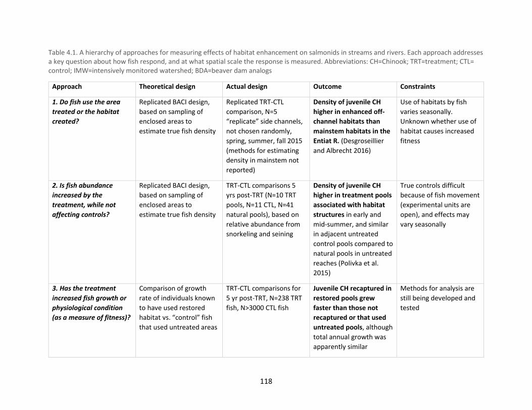
118
Table 4.1. A hierarchy of approaches for measuring effects of habitat enhancement on salmonids in streams and rivers. Each approach addresses a key question about how fish respond, and at what spatial scale the response is measured. Abbreviations: CH=Chinook; TRT=treatment; CTL= control; IMW=intensively monitored watershed; BDA=beaver dam analogs
Approach Theoretical design Actual design Outcome Constraints
1. Do fish use the area
treated or the habitat
created?
Replicated BACI design,
based on sampling of
enclosed areas to
estimate true fish density
Replicated TRT-CTL
comparison, N=5
“replicate” side channels,
not chosen randomly,
spring, summer, fall 2015
(methods for estimating
density in mainstem not
reported)
Density of juvenile CH
higher in enhanced off-
channel habitats than
mainstem habitats in the
Entiat R. (Desgroseillier
and Albrecht 2016)
Use of habitats by fish
varies seasonally.
Unknown whether use of
habitat causes increased
fitness
2. Is fish abundance
increased by the
treatment, while not
affecting controls?
Replicated BACI design,
based on sampling of
enclosed areas to
estimate true fish density
TRT-CTL comparisons 5
yrs post-TRT (N=10 TRT
pools, N=11 CTL, N=41
natural pools), based on
relative abundance from
snorkeling and seining
Density of juvenile CH
higher in treatment pools
associated with habitat
structures in early and
mid-summer, and similar
in adjacent untreated
control pools compared to
natural pools in untreated
reaches (Polivka et al.
2015)
True controls difficult
because of fish movement
(experimental units are
open), and effects may
vary seasonally
3. Has the treatment
increased fish growth or
physiological condition
(as a measure of fitness)?
Comparison of growth
rate of individuals known
to have used restored
habitat vs. “control” fish
that used untreated areas
TRT-CTL comparisons for
5 yr post-TRT, N=238 TRT
fish, N>3000 CTL fish
Juvenile CH recaptured in
restored pools grew
faster than those not
recaptured or that used
untreated pools, although
total annual growth was
apparently similar
Methods for analysis are
still being developed and
tested

119
4. Has the treatment
increased survival of fish
through one or more life
stages?
Barker capture-recapture
model to analyze a
replicated BACI design
Replicated TRT sites using
Barker model; N=8
“replicate” side channels,
not randomly selected, no
controls, 3 yrs post-TRT
sampling
Juvenile CH survival in
side channels was higher
during summer than
winter, and higher in
upstream than
downstream segments of
the Entiat River
(Desgroseillier and
Albrecht 2016; Grote and
Desgroseillier 2016)
Precise estimates of true
survival require sufficient
recaptures of permanent
emigrants (e.g., smolts;
Conner et al. 2015)
5. Has a set of treatments
increased smolt
production for an entire
population?
Estimates of smolt
production (smolts/redd)
for many years pre- vs.
post-treatment
No example found High sampling and
process variance on smolt
production estimates
limits power to detect all
but large differences pre-
vs. post-treatment. Effects
of habitat restoration are
confounded with those of
hatchery releases.

120
3. Has the treatment increased physiological condition or growth? – Physiological condition or
growth are more integrative measures of the importance of fish habitat than is abundance at a
point in time. Growth of juvenile salmon, for example, is known to confer advantages for
subsequent survival during smolting and ocean rearing. Therefore, a useful measure is to
compare whether the growth rate of individuals that were marked and recaptured during a
season in “restored” pools (those created by habitat restoration structures made from logs or
boulders) is greater than those that were marked in restored or unrestored pools and never
seen again (i.e., had no site fidelity near habitat structures).
Polivka and Mihaljevic (unpublished manuscript) reported that juvenile Chinook salmon in the
lower Entiat River that showed fidelity to restored pools (15-60 d between recaptures) reached
a larger size earlier in the season than those never recaptured, based on data from five
separate years during 2009-2016. Nevertheless, by the end of the growing season individuals
did not differ in length, regardless of habitat selection behavior. One explanation for this last
result might be that smaller fish that used unrestored habitat had higher mortality, although
this was not addressed by the authors.
4. Has the treatment increased survival of fish through one or more life stages? – A still more
integrative measure of fitness, and a key component for any population model, is survival.
Those fish that gain benefits from habitat restoration are expected to survive better during
periods when they are using treated areas as well as perhaps after they leave the area and use
other habitats. However, survival is estimated from marking and recapturing fish, so how can it
be measured for marked fish that leave, or for those that immigrate but are not marked? The
lack of information on these two groups could introduce unknown bias into estimates of
survival.
Recent advances in modeling data from capture-recapture sampling allow better estimation of
survival based not only on marking and recapturing animals in defined reaches, but also
detections beyond those reaches using fixed PIT-tag antennas, mobile PIT-tag detectors, or
other sources of recaptures. The Barker model (Barker 1997; Barker and White 1999; Conner et
al. 2015) has been successfully used to incorporate diverse sources of recaptures that occur
continuously in time (instead of only during discrete sampling occasions) to estimate true
survival that is not confounded with emigration, rather than only apparent survival where the
two are confounded, as estimated using Cormack-Jolly-Seber (CJS) models. As for all models,
the precision of these estimates increases when more fish are marked and more effort is
expended to detect both fish within reaches and those that emigrate permanently (e.g., smolts
that emigrate from the system; Conner et al. 2015).
121
Desgroseillier and Albrecht (2016) and Grote and Desgroseillier (2016) marked juvenile Chinook
salmon with PIT tags in six side channels along the Entiat River over 3 years, and detected them
in subsequent sampling as well as retrieving the detections at downstream dams during smolt
outmigration. Analysis revealed that their survival was higher during summer than winter, and
higher in side-channels farther upstream in the basin than those downstream. This method
holds promise to greatly improve the understanding of juvenile salmon survival through smolt
outmigration and has been successfully used in other Intensively-Monitored Watersheds for
juvenile steelhead (Bouwes et al. 2016). It is especially useful for steelhead, because they use
tributaries longer than juvenile Chinook and so are more frequently detected, and are more
likely to be detected as they emigrate permanently by smolting downstream (C. Saunders, Utah
State University, personal communication).
5. Have the entire set of habitat restoration treatments increased smolt production for a
salmon population? – The ultimate goal of habitat restoration is to increase the smolts per
redd, or smolt production, for the population of salmon in an entire subbasin, such as the
Wenatchee, Entiat, or Methow rivers. This requires measuring two quantities: the number of
redds produced each year for that population in the subbasin and the smolts that outmigrate
from the juveniles that emerge from those redds.
While conceptually simple, measuring these quantities is technically challenging and must be
conducted for long periods to have hope of detecting relevant changes owing to habitat
restoration (see below). Although estimating total number of redds is relatively
straightforward, based on stratified random sampling or complete census, it requires
substantial field effort. In contrast, measuring smolt output is done using floating screw traps,
which sample only a small volume of the outmigrant smolts, or with fixed PIT-tag antennas
located near the downstream ends of subbasins. As a result, the measurement variance on
estimates of smolts tends to be large (e.g., Grote and Desgroseillier 2017), and when added to
the process variance (e.g., natural fluctuations in smolt output year to year), results in large
total variances. The upshot is that many years of sampling before and after habitat treatments
are needed to detect even large changes in smolt production, based on power analyses (see
below).
At present monitoring is underway in the Upper Columbia subbasins to generate these data,
but they have not been analyzed to address whether there is evidence for a positive effect of
habitat restoration. Analysis in the Methow River subbasin showed that egg-to-emigrant
survival increased in the Twisp River over time, a tributary in which among the highest
proportion of habitat available and treatable had received habitat restoration (U.S. Bureau of
Reclamation Unpublished Data). However, there was also evidence for density-dependent
survival of spring Chinook emigrants and smolts in this tributary, suggesting that rearing habitat

122
or food may still be limiting. Overall, the problems described elsewhere with lack of suitable
control reaches, movement of fish among treatment and control reaches, the large extent of
treatments required to detect a response, and lag times for responses to occur remain difficult
challenges for detecting effects of habitat restoration.
The influences of density dependence and hatchery fish
Each of these measures of the success of habitat restoration may also be complicated by
density-dependent processes. For example, lower smolt output could result from too few
adults, or, alternatively, too many adults. In the former case, if segments or whole subbasins
are “under-seeded,” then the carrying capacity will not be achieved (see Bellmore et al. 2013
for an example in the Methow River, based on estimates of food production in floodplain
habitats), and the predicted responses to habitat restoration may not occur. In the second case,
high densities of adults can produce too many juveniles for the available carrying capacity,
which then survive poorly and reduce smolt output, owing to food, space, disease, or other
limitations at high densities, again confounding responses to habitat restoration.
Hatchery-reared juvenile salmon also increase density and place demands on food and space,
thereby contributing to density-dependent processes. A worst-case scenario is where these
hatchery juveniles usurp resources that would be used by wild juvenile salmon and yet have
lower fitness and die at greater rates at some life stage, thereby wasting resources that could
have supported wild salmon. Here again, this may eliminate some or all of the expected
response to habitat restoration.
4.2.2. Evidence of Fish Responses to Habitat Restoration of Key Limiting Factors
Key limiting factors for juvenile spring Chinook salmon and steelhead production have been
addressed by using seven main types of restoration actions grouped under the umbrella of
habitat: 1) removing barriers to connectivity, 2) increasing streamflow, 3) reconnecting
floodplains, side channels, and off-channel habitats, 4) restoring habitat complexity using log or
boulder structures, 5) managing fine sediment, 6) restoring nutrients, and 7) controlling
nonnative species.
Here we focus on evidence for fish responses to three types of projects that constitute the
majority of habitat restoration actions: restoring connectivity (13% of all projects; UCSRB
2014a), reconnecting floodplains and off-channel habitats (15%), and adding habitat structures
(21%). We address only briefly several other types of restoration projects (which together make
up 17% of projects) and do not discuss projects that address assessment and design (17%).
Habitat protection projects (the remaining 17%) are an additional category considered to be of
overwhelming importance and value by the UCSRB (2014b) and the Regional Technical Team in

123
their Biological Strategy (RTT 2014). The objective of these projects is to protect existing areas
with high ecological integrity where natural processes still occur. As of 2012, 46 projects were
completed that protected 3,379 acres (2,728 floodplain acres) and 47 miles of stream (UCSRB
2014b). It is clear that preventing degradation of habitat that is already functioning is among
the highest priorities, although it must be pursued judiciously, and not to the exclusion of
restoring other key habitats (RTT 2014).
4.2.2.1. Restoring connectivity
The UCSRB set a high priority on restoring connectivity by removing barriers to upstream
movement, or modifying them to become passible by fish, owing to the potential to allow
access to large amounts of habitat quickly. A recent report indicates that by 2012, 93 barriers
had been removed, opening 282 miles of previously blocked habitat (UCSRB 2014b). To date,
this one type of restoration restored far more length of habitat than all other types summed
together.
Success of projects that restore connectivity depends on the presence of suitable habitat
upstream, a downstream source population, and the distance upstream available for
colonization (Hillman et al. 2016). Studies within and outside the Columbia River Basin indicate
that colonization of upstream habitats opened to fish can be rapid, and that abundance is
similar above and below barriers after connectivity is established, indicating that fish have
recolonized the opened habitat. O’Neal et al. (2016) reported that fish passage projects in nine
rivers from across a wide range of river types in Washington and Oregon produced significant
increases in densities of juvenile coho salmon and all salmonids combined, based on
comparisons for 1 year pre-treatment versus 1, 2, and 5 years post-treatment, as well as
increasing post-treatment trends for these groups through time (P < 0.10 for each). However,
no such differences were detected for juvenile Chinook salmon. It is unclear at how many
locations Chinook salmon were present, which may have reduced the sample size for this
species and the power to detect the differences.
A good example of restored connectivity in the Upper Columbia is the modification of water
diversions to allow fish passage on Beaver Creek, a tributary of the lower Methow River,
although this project affected steelhead more than Chinook salmon. The diversions were
modified by creating rock-vortex weirs that impounded enough water to allow diversions for
irrigation, while simultaneously allowing fish to pass upstream. Many juvenile steelhead and
some juvenile Chinook salmon ascended the newly opened stream segment over the 4-year
monitoring period (Martens and Connolly 2010). During the final years of the evaluation adult
steelhead returned which had emigrated from the segment as parr, thereby confirming that an
anadromous population of this species had been re-established (Weigel et al. 2013). No
information was available on adult Chinook salmon returns.

124
Overall, studies from both within the Upper Columbia River region (UCSRB 2014b), and other
locations within and outside the Columbia River Basin (reviewed in Roni et al. 2008, 2014;
Hillman et al. 2016), have reported that colonization of newly opened habitat by anadromous
salmonids like spring Chinook salmon can be rapid and that densities can reach equilibrium
within a few years. Although few detailed studies of colonization were found for spring Chinook
in the UCR, this habitat restoration action remains among the highest priority and the most
certain to have positive biological benefits.
4.2.2.2. Reconnecting floodplains and off-channel habitats
Chinook salmon typically inhabit larger rivers with floodplains, and habitats in these off-channel
areas provide important rearing areas for many salmonids (Hillman et al. 2016). Restoration
projects may include reconnecting side-channels and off-channel ponds and wetlands,
removing or moving levees to allow channels to meander and connect with the floodplain, or
constructing off-channel habitats and restoring meanders. By 2012, more than 2700 acres of
off-channel habitat had been protected, 117 more acres reconnected, and 11 miles of off-
channel streams restored, representing the second largest number of restoration projects
(UCSRB 2014b).
In general, studies of the effects of these projects across the Pacific Northwest show rapid
recolonization of the newly accessible habitat by various salmonids (Roni et al. 2008; Hillman et
al. 2016). Chinook salmon are reported to use side channels fed by surface water more than
ponds or wetlands with little flow, at least in some regions (Pess et al. 2008).
Several studies in the Upper Columbia provide direct data on the biological benefits of off-
channel habitats for Chinook salmon and other salmonids. Desgroseillier and Albrecht (2016)
and Grote and Desgroseillier (2015) reported higher densities of juvenile Chinook salmon in six
off-channel habitats of the Entiat River (most were created or enhanced based on natural
floodplain features) compared to main channel habitats, indicating that fish colonized and used
the newly accessible habitats. Survival of juvenile spring Chinook salmon in the off-channel
habitats was similar during winter compared to summer (20% vs. 24%, respectively), despite
the harsher winter conditions. Moreover, survival in two off-channel habitats nearer the
headwaters was 10-15 percentage points higher during summer and winter than three of these
habitats near the river mouth, though the authors did not discuss reasons for the difference.
Upwelling groundwater sources common in floodplain habitats also enhance the food web that
supports Chinook salmon growth. Meija et al. (2015) reported that sites “gaining” groundwater
in the Methow River were warmer and had more nitrogen, periphyton, and benthic
invertebrates than sites in downwelling (“losing”) reaches. This resulted in nearly twice the

125
growth rate of hatchery juvenile Chinook salmon in enclosures during a field experiment, as
well as faster growth by free-ranging wild Chinook in gaining versus losing reaches.
Floodplains also store organic matter and nutrients deposited during floods, and so are rich
sources of production of invertebrates that feed fish. Bellmore et al. (2013) measured the
trophic basis of production for juvenile Chinook salmon, steelhead, and other fishes in five
floodplain channels of different types (e.g., a side channel connected downstream and a
disconnected channel not scoured by floods during the study). Based on extensive sampling and
analysis of fish (consumers) and their invertebrate prey, they found that in the main channel of
the Methow River about half to two-thirds of the production of invertebrate foods available to
support anadromous Chinook and steelhead was consumed by other native fish, including
mountain whitefish (Prosopium williamsoni) and several sculpin species (Cottus spp.).
Moreover, these non-target fishes consumed 95% of the total prey consumed by fish in this
habitat. In addition, production available to the anadromous salmonids in the side channels on
the floodplain was more than 2.5 times that in the main channel, even though much of it was
not used, apparently because of low densities of these anadromous salmonids (i.e.,
underseeding). This indicates that floodplain reconnection potentially provides additional food
resources to spring Chinook juveniles.
Following on this work, Bellmore et al. (2017) developed a model of the Methow River
ecosystem, the Aquatic Trophic Productivity Model, and used it to evaluate three restoration
scenarios: restoring riparian vegetation, nutrient augmentation by adding salmon carcasses,
and reconnecting side channels. Their results showed that reconnecting side channels had
much larger potential effects on native fish biomass (an estimated 31% increase) than carcass
addition (18%), and that riparian revegetation would have little effect (2%). However, this result
was altered in model runs that included, in addition, invasions by nonnative New Zealand
mudsnails (Potamopyrgus antipodarum) or potential nonnative fish predators such as
smallmouth bass (Micropterus dolomieu). Responses in fish biomass were still greatest for
reconnecting side channels, except in the worst-case scenario where both snails and fish
invaded, which reduced predicted fish biomass below that predicted for carcass additions
under this same invasion scenario.
Overall, restoring and reconnecting floodplains provides a wide range of benefits, especially for
rearing juvenile Chinook salmon, and is a high priority for habitat restoration. The models of
Bellmore et al. (2013, 2017) will prove useful to help managers think broadly about which
restoration actions are most likely to benefit target species like Chinook salmon and also to
compare their relative cost-effectiveness.

126
4.2.2.3. Adding habitat complexity using structures
Adding instream structures such as boulders and engineered log jams is the most common type
of habitat restoration project, making up more than a fifth of all projects including those for
habitat protection and for assessment and design. By 2012, these projects added 518
structures, created 180 pools, and enhanced 22 miles of stream in the UCR (UCSRB 2014b).
Despite this activity, adding habitat structures to rivers and streams has also received the
greatest scrutiny from restoration scientists, who often question whether they actually increase
fish numbers or biomass (e.g., Stewart et al. 2009; Whiteway et al. 2010; Roni et al. 2015). The
general hypothesis is that adding structural complexity to channels will increase survival during
summer and overwinter by providing refuges from flow, visual isolation from conspecifics and
aquatic predators, and overhead cover from terrestrial predators (Fausch 1993).
Although some analyses have reported equivocal effects (Stewart et al. 2009; but see
comments on flaws in this study by Whiteway et al. 2010), most report positive results overall
(Whiteway et al. 2010; Roni et al. 2015). For example, Hillman et al. (2016) reported that about
90% of the 83 studies they reviewed showed positive effects of placing habitat structures made
of large wood on physical habitat, and about 70-80% reported positive effects on juvenile or
adult salmonids (N=67 and 33 studies, respectively; Fig. 4.2), with less than 3% of studies
showing negative effects in any of these cases (the rest were equivocal). Even with an unknown
publication bias against negative results (i.e., investigators finding no effect or a negative effect
are unlikely to attempt publication or successfully publish results), these results are biologically
significant.
Likewise, it is unrealistic to expect that instream structures will improve physical habitat and
increase fish numbers or biomass equally in streams of all types across all biomes, just as we
would not expect all cancer drugs tested to be equally effective for all cancers or across all
patient groups (Mukherjee 2010). For example, O’Neal et al. (2016) showed positive effects of
adding structures on three characteristics of physical habitat (pool area, pool depth, volume of
wood), but no effects for juveniles of four salmonid species (Chinook, steelhead, coho, bull
trout), perhaps because the 12 projects they analyzed were scattered across various ecoregions
in Washington and Oregon. None were in the Upper Columbia River.

127
Figure 4.2. Proportion of published studies of placing structures made of large wood that reported positive effects, negative effects, or no change (equivocal) in physical habitat, fish (juvenile and adult salmonids, or non-salmonids), or macroinvertebrate density or diversity (Inverts). Number of studies (n) was 83, 67, 33, 17, and 21 for each case, from left to right. Some studies reported responses for several categories (from Hillman et al. 2016, after Roni et al. 2015).
Several studies provide direct data on the effectiveness of instream structures in the UCR.
Polivka et al. (2015) reported that pools associated with instream structures made of boulders
or logs had higher abundance of juvenile Chinook salmon during early and mid-summer,
compared to adjacent natural pools without structures, or natural pools in other nearby
segments with similar habitat. However, many of these juveniles were apparently summer
Chinook, which outmigrate by late summer, resulting in no detectable differences just
afterwards. Nevertheless, this work serves to address the concern that structures may draw fish
away from adjacent areas and argues for the view that the structures increase carrying capacity
rather than simply redistributing fish already present.
Roni et al. (2008, 2014, 2015) and Hillman et al. (2016) reviewed the large number of studies on
instream structures in other parts of the Columbia River Basin and beyond. The best example to
date of a comprehensive design and analysis for detecting the effects of instream habitat
structures on anadromous salmonids in the Columbia River Basin is the research conducted
under the CHaMP/ISEMP program in the Bridge Creek IMW in the John Day River basin of
central Oregon. Beavers create important habitat in this high-desert basin, and beaver-dam
analogs (BDA) have been used there to mimic the effects of beaver dams as well as to
encourage beavers to build their own dams (Pollock et al. 2014).
0%
10%
20%
30%
40%
50%
60%
70%
80%
90%
100%
Habitat Juv. salmonids Adult salmonids Non-salmonids Inverts.
Positive Negative Equivocal

128
A 7-year field experiment based on a BACI design, including four replicates of treatment
reaches with BDA and three reference reaches in a similar watershed nearby (which, therefore,
were fully independent) was used to measure the density, growth, survival, and production
(g/m/day) of juvenile steelhead in response to the beaver dam analogs (Bouwes et al. 2016).
Fish were PIT-tagged in study reaches but also detected with fixed and mobile PIT-tag antennas
in other reaches and downstream locations, allowing use of the Barker model (a modification to
the Cormack-Jolly-Seber model for open populations) to estimate true survival rates. Analyses
detected much greater density of juvenile steelhead (an increase of 81 fish/100 m), lower
growth (owing to density-dependence, given the higher density), a 52% increase in survival, and
a 175% increase in juvenile steelhead production in the treatment reaches compared to those
in reference stream reaches. In addition, the structures moderated diel temperatures because
of increased water storage and interaction with groundwater, benefiting salmonids by buffering
temperature extremes and providing thermal refuges (Weber et al. 2017). This example from
the CHaMP/ISEMP program is one of the most comprehensive and successful evaluations of
instream structures completed for an anadromous salmonid population to date, anywhere in
the world.
4.2.3. Application of Life-Cycle Models to Integrate Habitat Restoration with
Other Effects
An important goal of the UCSRB is to use Life Cycle Models (LCM) to analyze the effects of
habitat restoration that is coincident with other effects likely to be caused by hatcheries,
hydropower, harvest, and variable ocean conditions (see Roni et al. in press for review of
methods for assessing habitat restoration). Toward this end, the CHaMP/ISEMP group is
developing a LCM for the Entiat River, which is also an Intensively Monitored Watershed (IMW).
The Entiat River IMW was established in 2011, and habitat projects were conducted in 2012
and 2014. Saunders et al. (2017) reported on development of a LCM and its use in a preliminary
analysis, which is similar to the LCM developed for the John Day River IMW. They used this
model to analyze the effects of a subset of the habitat projects conducted in 2012 in the Entiat
River. The analysis showed that this subset of projects increased rearing capacity for juvenile
Chinook (spring and summer runs combined) an average of 7% across the sites treated,
amounting to a <1% increase in carrying capacity for the whole basin. When combined with an
assumed 2% increase in overwinter survival expected owing to the restoration, the predicted
abundance of spawners increased about 25%, from about 230 to 290, but not enough to reach
the goal of 500 spawners set in the Recovery Plan.
Despite these model assumptions and predictions, the analysis of empirical data to date
detected no change in juvenile Chinook salmon survival, and also had low statistical power to
detect changes in abundance (S. Walker, TerrAqua, personal communication). A post-hoc

129
analysis of statistical power indicated that, given the variability measured to date, only very
large year-over-year changes in Chinook abundance (i.e., >60%) owing to restoration could be
detected with statistical confidence. A further analysis using the LCM to estimate the increases
in current habitat capacity and survival needed to reach the recovery goal of 500 spawners
indicated that a 10% increase in each was predicted to meet the goal, and that a 5% increase in
each might achieve the goal.
Firmer conclusions from this work must await further analysis of the habitat actions completed
to date. However, the preliminary results from the IMW in both the John Day and Entiat rivers
(Saunders et al. 2017) indicate that the habitat restoration scenarios evaluated to date,
especially those using log and boulder structures, are unlikely to have sufficiently large effects
alone to increase either habitat capacity or survival enough to reach recovery goals. Although
adding habitat complexity using these structures is an important objective as part of a
comprehensive habitat restoration strategy, the relatively larger biological effects of restoring
fish passage by removing barriers and restoring and reconnecting floodplains are likely to be
more important goals in the near term. Likewise, managing riparian zones and uplands to
deliver large wood, and managing channel geomorphology to allow storing it in floodplains and
channels, are important long-term goals.
4.2.4. Sample Designs and Sample Sizes Needed to Detect Biologically Significant
Effects
Data on fish abundance, growth, survival, and smolt production are inherently variable, owing
to both sampling error (variability owing to the sampling process) and process error (e.g.,
annual variability due to years with different temperature or flow regimes). Process error is
often much greater than sampling error, so many years of data are needed to detect effects
with acceptable statistical power and confidence, even in a simple design comparing effects
before vs. after habitat restoration.
If a BACI design can be used, perhaps by employing an adjacent control basin like the Chiwawa
River basin used for the Entiat River IMW (S. Walker, personal communication), the analysis is
more complex. In summary, however, with as much as 5 years of data for the periods before
and after the treatment, and typical levels of sampling and process error, it is likely that only a
doubling or halving of abundance could be detected with acceptable statistical power and
confidence (see Appendix E for discussion of BACI designs).
In a similar analysis, Paulsen and Fisher (2005) reported that given five control sites and three
treatment sites at which 10 years of data were collected before habitat manipulations and 7-9
years of data collection occurred afterwards, an investigator can detect a 30% increase in parr-

130
to-smolt survival (based on tagging juveniles and detecting them at a downstream dam) at
acceptable levels of statistical power (80%) and significance (alpha=0.05).
This example shows that a key requirement is a long run of pre-treatment data, which is
counterintuitive to most practitioners and unlikely to be available or planned. That is, when
funds are available for habitat restoration, most practitioners want to complete projects, rather
than wait to measure pre-treatment data and risk losing funds. However, O’Neal et al. (2016)
showed that for analyses of habitat restoration, adding 1 year of pre-treatment measurements
increased the power to detect differences more than including up to 100 years of post-
treatment data. Increasing pre-treatment data from even 1 year to 2 years improved power by
about 30%, and 5 years of data before and after treatments appeared optimal.
4.3. Approaches for Prioritizing Habitat Projects
4.3.1. Ecosystem Diagnosis and Treatment (EDT) Model
The Ecosystem Diagnosis and Treatment (EDT) model is a life-cycle habitat model that can
characterize salmonid ecosystems temporally and spatially (ICF International 2017; Roni et al. in
press). The model is built to assess salmon performance in terms of capacity (i.e., maximum
population size), productivity (i.e., survival at low density), and diversity (i.e., life history
trajectories linked to coordinates of time and space; Mobrand et al. 1997). EDT uses a multiple-
stage Beverton-Holt production model with species and life-stage specific performance
benchmarks for optimal environmental conditions (Blair et al. 2009). The environmental
conditions considered include physical habitat and water quality conditions as well as food
availability.
To characterize the environment, life stage survival factors are derived from environmental
attributes based on raw data that comes from field data (preferred), information derived from
other attributes, expert opinion, or hypotheses (Blair et al. 2009). Environmental attributes
include hydrologic characteristics (e.g., flow, hydrologic regime), stream habitat structure (e.g.,
channel morphometry, habitat type, obstructions, sediment), water quality (e.g., chemistry,
temperature), and biological community effects (e.g., biotic interactions with competitors,
predators, parasites and pathogens, and macroinvertebrates). The model also considers the
percent of key habitat (i.e., primary habitat types such as pools, glides, riffles) for different life
stages within each geographic unit, and a food factor that incorporates alkalinity, benthic
community richness, riparian function, and salmon carcasses. The life stage survival, key
habitat, and food factors are used to adjust the performance benchmarks to evaluate current
or potential habitat scenarios (Blair et al. 2009). The results can be related to the Viable
Salmonid Population (VSP) criteria of McElhany et al. (2000; see Arterburn 2017; ICF
International 2017).

131
The EDT model was used for the Fish and Wildlife Program’s 2004 Subbasin Plans for the Entiat,
Methow and Okanogan watersheds (see plans for each basin in
www.nwcouncil.org/fw/subbasinplanning ). More recently in the Upper Columbia Basin, the
Okanogan Basin Monitoring and Evaluation Program (OBMEP) has been integrated with EDT to
track trends in data quality and data collection needs, identify priority areas for habitat
protection and restoration, provide a method for evaluating biological effectiveness of
restoration actions, and to evaluate strategies for reintroducing extirpated species (Colville
Confederated Tribes 2013). In collaboration with the Colville Confederated Tribes, ICF
International has developed Salmonid Population Report Cards for populations and reaches to
visually summarize OBMEP data and EDT output (Colville Federated Tribes 2013; Arterburn and
Klett 2015; Arterburn 2017; Eric Doyle, ICF International, personal communication).
EDT modules can be downloaded without charge. However, the development of an EDT
application for a particular basin requires an initial investment with ICF International who
currently maintains the software. For example, an EDT application for the Methow River basin
was started in 2016, with the initial release expected in early 2018. Developing the Methow
EDT model involved upgrading the EDT model for the Methow Subbasin Plan to the latest
version of EDT, reconfiguring the reaches based on lessons learned from the Okanogan EDT
model, and incorporating new habitat data collected since 2004. The approximate cost for
developing the Methow EDT model is $250,000. Once the application has been built,
maintenance costs of $100,000 per monitoring cycle are likely (Eric Doyle, ICF International,
personal communication), although the costs decline over time as model use is standardized in
a basin (e.g., monitoring cycle costs in the Okanogan are estimated at <$60,000; J. Arterburn,
Colville Tribes, personal communication).
4.3.1.1. Applicability of EDT for ranking of habitat projects
The EDT approach seems well suited to ranking and evaluating the effectiveness of habitat
projects. It has the advantage of incorporating food availability, and the authors suggest that it
can be linked to other models of land use that predict input variables to EDT like sediment,
thereby addressing factors advocated by ISAB as important for assessing salmon recovery (ISAB
2011-1; ISAB 2011-4; Naiman et al. 2012). The approach incorporates rule-based relationships
between species survival and environmental characteristics that are based on prevailing
scientific knowledge (ICF International 2017). It is able to evaluate the habitat needs for
discrete life stages and has been designed to provide data that relate to VSP criteria. The model
can be used to indicate reaches and actions that could improve VSP criteria, thus providing a
means to prioritize actions.
ICF International (2017) is clear that the model is not a predictive model (i.e., it does not
forecast future conditions), and it is difficult to validate the model against measured data (Steel

132
et al. 2009). A review of subbasins plans by ISAB and ISRP concluded that EDT results can be
considered hypotheses that should be tested (ISAB/ISRP 2004-13). Thus, it seems plausible that
if long-term monitoring of fish responses and environmental conditions is done after projects
are implemented, then empirical estimates of the VSP parameters could eventually be
compared against predictions from the model to validate them, and indicate model parameters
that require refinement. ICF International (2017) describes this type of validation exercise
conducted for five steelhead and four salmon populations (Rawding 2004). Model estimates of
productivity (alpha) and capacity (beta) for the Beverton-Holt curve were within the 95%
confidence limits for the nine populations.
In the Okanogan Basin, removal of culvert barriers and an irrigation knife gate on Loup Loup
Creek enabled fish passage in 2014. The EDT model had estimated that the additional habitat
should support an adult abundance of 27 summer steelhead, and in 2014, exactly 27 wild
summer steelhead returned to the assessment unit. Over time, the EDT model predicted a 5-
fold increase in juvenile abundance with the restoration actions on Loup Loup Creek, but
OBMEP has found an increase closer to 10 times the abundance prior to restoration (J.
Arterburn presentation to ISAB, July 20, 2017). Although in this case the EDT predictions of
adult abundance happened to be the same number of steelhead seen in 2014, EDT estimates
should be considered as relative, rather than absolute estimates (ISRP/ISAB 2004).
Sensitivity analyses were performed on EDT by the U.S. Bureau of Reclamation (Reclamation),
Washington Department of Fish and Wildlife (WDFW), and NOAA Fisheries (Steel et al. 2009;
McElhany et al. 2010). Steel et al. (2009) reported that Reclamation found that EDT was
relatively insensitive to flow attributes in the Yakima basin, which were important to their
decision-making, so they developed additional models to predict values for several habitat and
temperature attributes incorporated in EDT that are most influenced by changes in stream
flow. A sophisticated sensitivity analyses conducted by NOAA Fisheries indicated that prediction
intervals for estimates of abundance, productivity and capacity had large ranges, leading
McElhany et al. (2010) to caution against using EDT for management decisions that require a
high degree of confidence in these outputs, such as setting harvest limits or endangered species
goals. However, the model was fairly robust in ranking the highest-priority reaches for
preservation or restoration (Steel et al. 2009; McElhany et al. 2010), so it is likely to be useful
for this goal in the Upper Columbia. McElhany et al. (2010) also reported that the model
required a large amount of time to calculate outputs for the sensitivity analysis, which could be
a constraint for model users.
One concern reported by McElhany et al. (2010) was the limited ability for model users to
adjust some input parameters. ICF International has revised the model since the assessments
by McElhany et al. (2010) and Steel et al. (2009) to create a more modular structure to the

133
model that allows the rule structure of the model to be modified (Eric Doyle, ICF International,
personal communication). The presentation by Arterburn (2017) to the ISAB indicated that the
Okanogan River application of EDT has incorporated adjustments to input parameters.
Additionally, because OBMEP raw data are integrated with EDT, the model can be part of an
adaptive management strategy to refine and update the relationships between environmental
attributes and survival factors. EDT includes a rating for the quality of Level 1 data (i.e., raw
data and observations), noting that empirical field data are the most desirable (Blair et al. 2009;
Colville Federate Tribes 2013). The OBMEP report cards provide an overview of data quality so
that progress can be tracked on obtaining data for the models. The report cards also show
progress towards goals as well as priorities of projects both spatially and by project types.
Another concern reported by ISRP/ISAB (2004) was the limited application of EDT for hatchery
interactions. EDT does include hatchery releases in its accounting for density dependence and
competition. For more detailed assessment of hatchery-wild interactions and impacts to
populations, the Colville Tribes uses the productivity and capacity values from EDT with the All-
H Analyzer (AHA) spreadsheet model (J. Arterburn, Colville Tribes, personal communication).
The AHA model is available from Lars Mobrand (see Appendix G of ICF Jones & Stokes 2010 for
a description).
Should EDT continue to be developed and applied in the Upper Columbia Basin and the rest of
the Columbia River Basin, a scientific evaluation of the species habitat rules might be prudent.
At the time that EDT was developed in the 1990s, much less data were available to establish the
rules. Satellite imagery, monitoring data, and data from experimental studies could be useful
for revising or updating EDT rules.
4.3.2. Habitat Suitability Indices (HSI)
Habitat suitability index (HSI) approaches were initially developed in the 1980s (Roloff and
Kernohan 1999). For aquatic species, HSIs typically represent preferences of each species for
instream variables (e.g., velocity, depth, substrate, and cover) at different life stages (Ahmadi-
Nedushan et al. 2006). Indices generally range from 0 (no preference) to 1 (maximum
preference) for a particular habitat condition and can be combined to develop a composite
suitability index. For example, depth, velocity and cover HSIs might be combined by multiplying
the individual indices, which would result in zero suitability if any of the variables were
considered unsuitable (Ahmadi-Nedushan et al. 2006). Such composite indices assume that all
variables are equally important and that all environmental variables are independent with no
interactions. To address the first assumption, weights can be used to incorporate relative
importance of variables. However, interactions among variables cannot be addressed with HSI
(see Ahmadi-Nedushan et al. 2006 for an analysis of several alternative approaches to HSI to
address interactions).

134
There have been criticisms of HSI models used for evaluating habitat and population responses
to habitat quality (Roloff and Kernohan 1999; Ahmadi-Nedushan et al. 2006). Although the
models do quantify habitat suitability, this metric may or may not be directly correlated to fish
abundance and biomass (Rose et al. 2015) because other factors like food may have overriding
effects. As Booth et al. (2016) point out, more habitat does not guarantee desired biological
gains, especially if a clear understanding of the relationship between habitat and the life history
of the target species is lacking. Roloff and Kernohan (1999) assessed 58 HSI model validation
studies and found that the applications failed to account for variability in input data, which in
turn affects HSI output interpretation. Other shortcomings noted were model applications at
inappropriate spatial scales, inability to account for density-dependent effects, and lack of
sufficient duration of observations to test model performance (Roloff and Kernohan 1999).
In the mid-Columbia River Basin, McHugh et al. (2017) applied a spawning HSI to estimate
spawner capacity in egg equivalents for steelhead in the Middle Fork John Day Basin. This HSI
model was used with inputs of flow depth and velocity from a hydraulic model (Delft3D) to
assess the quality of spawning habitat across space within reaches. The spawning capacity was
then upscaled from reaches to the entire basin using statistical modeling based on bankfull
width. The demographic parameters predicted from these analyses were used as input to the
life-cycle model (LCM) for the basin. The combined models were used to assess riparian
restoration scenarios that considered 1) baseline (or status quo) conditions, 2) best-case
riparian revegetation, channel adjustment, and instream flow acquisition, 3) complete
maturation of current (i.e., 2008) vegetation, and 4) targeted placement of instream wood
structures. This modeling effort also included use of a net rate of energy intake (NREI) drift-
foraging model of juvenile steelhead habitat capacity (McHugh et al. 2017). A similar approach
has been used by Saunders et al. (2017) in the Entiat River basin for spring Chinook. Use of an
HSI model for spawner capacity may be among the best applications of this method, because
fish are selecting habitat for a defined period based on a few key variables that can be
measured and modeled (i.e., depth, velocity, substrate, and cover).
In the Upper Columbia Basin, HSI models have only been applied at the spatial scale of
individual projects. Welch (2017) described the use of HSI models with hydraulic models for
project selection and design, indicating that Bonneville Power Administration (BPA) would be
requesting this type of analysis as part of statements of work. They noted that HSI models were
useful for bridging the gap between biologists who could identify habitat suitability criteria and
engineers who needed to design projects.
Busch et al. (2013) developed an intrinsic potential (IP) model for spawning fall Chinook salmon
in the Lower Columbia River evolutionarily significant unit (ESU) that is a variation of habitat
suitability models (see Roni et al. in press for descriptions of these model types). Their IP model

135
described potential habitat by using 10-m digital elevation models to rate habitat
characteristics of channel confinement, channel width, and channel gradient. Busch et al.
(2013) performed a sensitivity analysis of the shapes of suitability curves and found that results
for some watersheds were very sensitive to curve shapes. Correlations between model results
and available fish abundance data at the population level were not significant, and they were
unable to examine the ability of the model to predict fish data spatially due to lack of data.
Nevertheless, output from the IP model was significantly correlated with corresponding EDT
output at the reach and population level.
4.3.2.1. Applicability of HSI for ranking of habitat projects
The HSI-LCM applications in the Middle Fork John Day Basin were designed to assess what type
of restoration project (e.g., riparian restoration, addition of wood) was better suited to improve
population abundance of steelhead, but the applications did not appear to be used to prioritize
placement of such projects (McHugh et al. 2017). Welch (2017) indicated that HSI models
coupled with hydraulic models would be required for project selection and design in the Upper
Columbia Basin but did not describe how these approaches would be used to prioritize habitat
projects (e.g., what criteria would be used, how projects would be evaluated). Roni et al. (in
press) provide a comprehensive review comparing methods used to prioritize habitat
restoration.
4.3.3. Regional Technical Team (RTT) Biological Strategy
The Upper Columbia Regional Technical Team (RTT) started as an ad-hoc group of scientists
who wanted to coordinate and prioritize restoration actions (Kahler 2017). Representatives of
the agencies involved have agreed to “check their agency affiliations at the door.” The RTT
Biological Strategy involves using what they term planning science, review science, and
adaptive management in salmon recovery. Planning science involves using tools like ecological
models (e.g., EDT, Shiraz, Physical Habitat Simulation [PHABSIM], and life-cycle models), reach
assessments, published literature, and local research and expertise to identify limiting factors,
improve the biological strategy, inform recovery plans and habitat actions, and develop the RTT
priorities spreadsheet. Reviewing science involves RTT evaluation of projects once they have
been proposed. As part of adaptive management, the RTT synthesizes monitoring and makes
recommendations to the UCSRB, regional co-managers, and the Upper Columbia River
Umbrella Project (Kahler 2017).
The RTT’s Biological Strategy (RTT 2014) states that the highest priority for protecting biological
productivity is to sustain natural geo-fluvial processes, such as unrestricted channel migration,
floodplain function, and adequate stream flows, especially when these processes are already
functioning at a high level. In contrast, the highest priority for increasing biological productivity

136
is to restore stream channel complexity and floodplain function. The RTT recognizes that there
must be a pragmatic balance between protection and restoration actions, with recovery as the
goal.
The Biological Strategy includes a description of how projects are prioritized and rated. The
major subbasins in the UCR (Wenatchee, Entiat, Methow, Okanogan) are divided into
assessment units, each of which is a portion of the subwatershed (e.g., lower Wenatchee River)
or a tributary (Nason Creek). Assessment units are assigned one of four priorities, with the top
priority assigned to areas with high quality functioning habitat. Within these units, protection
and restoration actions are defined in two tiers, with the top tier designating the highest
priority actions that could be accomplished under ideal conditions, such as when most land
ownership is public. For example, Tier 1 protection actions protect high-quality geo-fluvial
processes, and Tier 1 restoration actions restore fluvial geomorphic processes. The report has
tables that indicate the priorities for addressing ecological concerns (i.e., limiting factors) for
each assessment unit, although coordination of the priorities with the Viable Salmonid
Population (VSP) criteria was not clear.
4.3.3.1. Assessment of RTT Biological Strategy for prioritization of habitat projects
The ISAB raises two major concerns about the ranking criteria used to prioritize projects.
Analysis of cost-effectiveness is not quantitative and is given a low weighting in the final
rankings. Potential projects are ranked sequentially by two groups within the UCSRB. First, cost
effectiveness is considered, but only after the technical criteria have been scored. The RTT
developed two scoring rubrics to assess priorities for protection projects and restoration
projects. For protection projects, seven criteria are scored and weighted, with the highest
weights given to criteria protecting habitat at locations important to fish and protecting
habitats that would result in the greatest loss of freshwater habitat capacity or fish survival if
they were lost. For restoration projects, 10 criteria are scored and weighted, with most weight
on criteria considering how well projects address the ecological concerns (i.e., limiting factors),
whether they are appropriately located and scaled, and the expected benefits to habitat
capacity and fish survival. Several criteria also address the lag time before benefits of
restoration projects are expected and the duration they will persist. However, for each rubric,
cost effectiveness is considered in imprecise terms, but not explicitly calculated, and makes up
only 5% of the total score. The project rankings by the RTT are then submitted to the Citizens’
Advisory Committee, which considers benefits to fish (the RTT ranking; 40%), project longevity
(20%), project scope (10%), community support (17%), and economics (13%). As with the RTT,
the cost effectiveness analysis is not quantitative and is given a low weight. Final funding
decisions are made by the UCSRB and the Salmon Recovery Board of the state of Washington.
Reportedly, cost effectiveness is considered by these regional entities, but there is no explicit
analysis and the evaluations are not documented. Independent estimates of cost-effectiveness

137
metrics, like those described in section 4.1, are not calculated in either local or regional
rankings and decisions.
The second major concern is the lack of a formal approach for weighting both cost and time
elements of projects. As discussed in Section 4.1, projects that produce benefits sooner rather
than later, over a much longer period, or at a fraction of the cost of other projects, need to be
weighted proportionally to allow maximizing objectives within constraints of limited time and
resources. Cost differences between projects are as important as benefit differences for
achieving program objectives. Cost-effectiveness should be determined using the ratio of
biological benefits (in ecological units) to costs (in monetary units), instead of implicitly
addressing them in other scoring components. Providing resources equally among geographic
units instead of accounting for the relative cost effectiveness of different actions can lead to the
lowest possible benefits to society (Wu et al. 2003).
Coordination of the priorities with the Viable Salmonid Population (VSP) criteria also was not
clear. Despite the understandable hesitation to estimate the numbers of additional fish that a
project will produce in years 1-10, 11-25, and 26-50, those estimates are needed to be able to
give more weight to benefits that come sooner rather than later, by discounting future benefits
(see Section 4.1.2). These time-weighted estimated benefits are then divided by project costs to
produce a time-weighted measure of benefits per dollar of cost. This metric allows prioritizing
projects to achieve the greatest overall benefit for the lowest cost in the shortest time period.
Similar methods are required for projects in most federal and state agencies (EPA 2010).
4.4. Coordination and Interactions with Other Hs
The Upper Columbia Salmon Recovery Board (USCRB) works with partners to facilitate recovery
actions in the Wenatchee, Entiat, and Methow basins, including creating an overall operational
structure, developing explicit strategies, and coordinating actions. The UCR Recovery Plan for
spring Chinook salmon is designed to increase the capacity of the habitat to produce
outmigrants (smolts/redd), resulting in greater numbers of returning adults (UCSRB 2014b).
However, other limiting factors such as mortality during downstream migration, poor ocean
conditions, or predation may reduce these benefits. Hence, habitat actions must be
coordinated to complement actions in other sectors and address the most important limiting
factors and interactions among factors.
The UCSRB has developed one of the better examples of a well-documented process for
prioritizing restoration projects and coordinating recovery actions within groups responsible for
habitat, hydrosystem, hatcheries, and harvest. The regional recovery plan, improved limiting
factor assessment, life-cycle models, and monitoring provide critical information for recovery
actions for spring Chinook salmon. One of the greatest challenges for the UCSRB is coordination
138
of the different groups in the three basins that are responsible for the different Hs. Currently,
there is no process for regularly discussing the findings and actions of the different groups and
integrating the separate efforts into a coordinated action plan.
4.4.1. Operational Structure
As described for the prioritization of recovery actions, the UCSRB has the responsibility to
develop the Recovery Plan for the UCR and coordinate habitat actions with hatchery
operations, harvest, and hydropower (www.ucsrb.org/). The RTT developed the Upper
Columbia Biological Strategy as a regional framework for developing actions to recover native
salmonids stocks (RTT 2014). The RTT provides the technical basis for the regional strategy and
reviews habitat projects at several stages of development and implementation.
Coordination by the UCSRB also considers all watershed plans in the Upper Columbia Region to
address habitat objectives of the recovery plan
(www.digitalarchives.wa.gov/GovernorLocke/gsro/regions/upper.htm). The UCSRB submits
project lists to the Salmon Recovery Funding Board of the state of Washington. In addition, the
Board receives funding for habitat actions through the Umbrella Projects of the NPCC. Counties
and co-managers lead the implementation of the subbasin plans. The UCSRB attempts to align
local watershed plans and the regional subbasin plans into the regional salmon recovery plan.
4.4.2. Strategies
Creating the Recovery Plan relies on integrating actions across all sectors affecting salmon and
steelhead (harvest, hatcheries, hydropower, and habitat) as well as integrating actions beyond
the boundaries of the Upper Columbia region (e.g., lower Columbia, estuary, and ocean). While
the Recovery Plan includes specific actions for habitat, it acknowledges that actions in
freshwater tributary habitat are not likely to achieve recovery on their own and should not be
the sole focus of recovery efforts. Achieving viable salmonid populations requires recovery
actions across all H-sectors.
Management of salmon and steelhead requires coordinated decision-making to achieve
recovery while honoring treaty and reserved rights and meeting legal and regulatory
requirements. The UCSRB developed an Integrated Recovery Program to align management
and restoration actions across all entities involved in UCR salmon recovery. The Integrated
Recovery Program tracks and reports information about actions implemented for recovery of
salmon and steelhead across management and geographic boundaries. Habitat Reports
document project results, recent outcomes to support “All-H” collaboration, and progress
toward integrated recovery.
139
The UCSRB established the Upper Columbia Programmatic Habitat Project (UCPHP) to
implement reach-based habitat restoration projects in high-priority areas in the Upper
Columbia Region (Umbrella Project). The UCPHP coordinates regional actions to meet
mitigation obligations under the 2008 FCRPS Biological Opinion (BiOp) with recovery needs and
priorities identified in the Upper Columbia Spring Chinook Salmon and Steelhead Recovery Plan
(Recovery Plan; UCSRB 2007), and the Biological Strategy (UCRTT 2013).
The Recovery Plan of the UCSRB includes a general analysis of the benefits of salmon recovery
and the economic costs of recovery actions to other sectors in the region (Chapter 6
Social/Economic Considerations, p 250). The economic benefits of recovery of salmon and
steelhead were quantified based on economic information and analyses from the Columbia
River Basin, including the Snake River basin. Economic costs were quantified for the agricultural
sector of the three basins. Although the RTT review process provides relatively limited
information on cost effectiveness of specific projects, the UCSRB as a whole includes some
consideration of the economic factors associated with salmon recovery.
4.4.3. Coordinating Actions
The UCSRB tries to be informed about the individual strategies related to habitat, hydrosystem,
hatchery, and harvest working groups, but coordination of the different groups that have been
working for more than 20 years is complex. The UCR includes a substantial number of separate
coordinating committees that are independent and report to different entities. Each of the
Habitat Conservation Plans (HCPs) for Chelan and Douglas PUDs has a Coordinating Committee,
Hatchery Committee, and Tributary Committee. Grant County has the Priest Rapids
Coordinating Committee, a Hatchery Committee, and a Habitat Committee. The RTT also
coordinates habitat assessments and actions in the UCR. There is no coordinating committee
for harvest actions in the UCR. Each PUD also has a separate committee to address issues
related to non-native invasive species. While membership overlaps on the coordinating
committees and some of the committees have joint meetings, the ISAB understands that
decision-making processes are separate and reporting and coordination between the
committees is not systematic.
The UCSRB meets regularly and includes participants from the habitat, hatchery, hydrosystem,
and harvest sectors who review future projects and coordinate actions. The RTT also meets
regularly to review information and coordinate activities. Reviews by the RTT provide some
communication between habitat and hatcheries, and to some degree harvest, but there is no
systematic coordination of the actions between the RTT and the PUDs. The PUDs provide
important funds for hatchery and habitat because of funding obligations of the PUDs based on
responsibilities for impacts related to the reservoirs, dams, and tailraces. The PUD operations
are assumed to lower survival of salmon and steelhead passing through the hydrosystems of
140
the upper Columbia River by up to 9%, 7% for juvenile mortality, and 2% for adult mortality.
Licensing agreements require the PUDs to mitigate for 7% of the 9% decrease in survival and 2%
is mitigated by habitat restoration actions (FERC 2002). The PUDs provide funds for the
hatcheries and monitor hatchery releases to document the hatchery mitigation. The 7%
mitigation obligation can be reduced by improving survival from upstream rearing areas
through the dams, which is monitored annually and adjusted based on 4-yr averages. They also
provide funds for habitat restoration projects in the basin, but the outcomes are not assessed
and monitoring for habitat conditions and fish-habitat relationships is not specifically funded.
Hatchery managers and co-managers are involved in coordination with hydrosystem operations
and are funded in large part by hydrosystem obligations. Though managers of the hydrosystem
and hatcheries actively participate in the RTT, hatchery operations potentially influence the
effectiveness of habitat restoration actions. Studies in the UCR have found that hatchery
releases potentially reduce fitness of juvenile spring Chinook (see Chapter 5), which would
reduce the effectiveness of habitat restoration. Continued management refinements to reduce
effects of hatcheries on fitness of spring Chinook in the three basins must be coordinated with
habitat restoration projects to improve recovery efforts.
The Recovery Plan is designed to coordinate habitat restoration actions with harvest. Both
ocean and in-river harvest in the Columbia River basin are coordinated and managed through
the United States v. Oregon Management Agreement under the jurisdiction of the federal
court. Harvest intercepted 5 to 18% of returning spring Chinook salmon during 1977 to 2013
(NOAA Salmon Population Summary database). Washington Department of Fish and Wildlife
(WDFW) recommends harvest levels for UCR stocks within this Management Agreement.
WDFW reports their harvest management plans to the RTT and UCSRB, but there is no major or
regular process for feedback from the RTT and UCSRB to harvest management decisions.
Though the Management Agreement ultimately determines the degree to which harvest
influences numbers of returning adults, collaborative discussions of the influence of adult
return rates on spring Chinook recovery in the UCR and potential harvest management options
would strengthen recovery efforts of the UCSRB.
4.5. Recommendations
Here we address the questions posed by the Council, after rearranging them to group several
similar ones together:
Are habitat recovery actions being prioritized and sequenced strategically, given
existing knowledge and data gaps? How should habitat projects be prioritized?
The ISAB found the UCSRB’s system for soliciting, reviewing, and designing restoration projects
to be scientifically sound with regard to habitat conditions and effects of hatcheries and the
141
hydrosystem. Assessments of limiting factors are used to prioritize recovery actions, and the
recent history of restoration is relatively consistent with the rankings of limiting factors. Current
methods of prioritization (e.g., EDT, HSI, RTT Biological Strategy) are useful.
The life-cycle models that have been developed for the three UCR basins show great potential
for integrating multiple factors that determine the abundance of spring Chinook throughout
their life histories and across their full geographic range. The recent ISAB review of the life-cycle
models (ISAB 2017-1) commended the recent progress of the life-cycle modeling effort and
expansion to new areas in response to previous ISAB recommendations. The ISAB review noted
that models are always a tradeoff between realism and simplicity and do not include all sources
of variation. They concluded “the models can be used for ranking scenarios, but their predicted
results may not be accurate.” The capacity to rank scenarios and integrate multiple factors
across the full life history of spring Chinook strengthens the prioritization of projects and
coordination of actions across participants in the UCSRB Recovery Strategy.
The UCSRB focuses most attention on determining which kinds of actions will be biologically
beneficial toward recovery of Upper Columbia spring Chinook and assesses fish abundance,
productivity, and risk of extinction. The procedure for characterizing cost effectiveness is not
quantitative and does not provide a rigorous basis for prioritizing actions. If funds are unlimited,
there would be no need to prioritize actions, but that clearly is not the case. The criteria used
by the RTT and the Citizens Advisory Committee are vague and the results are weighted, so
they have little influence on project priorities. Cost effectiveness is considered by the UCSRB
and the Salmon Recovery Board, but there is no explicit analysis and the evaluations are not
documented.
The ISAB recommends applying a transparent cost-effectiveness analysis of each project
proposed, perhaps by using the approach in the simple example we described (see section
4.1.2) as a starting point. The lack of rigorous cost effectiveness analysis and its minor influence
on prioritization of restoration actions for all Hs limit the USCRB and participants in their
recovery efforts. This is a common deficiency throughout the Columbia Basin, but such analyses
would allow the program to use its limited resources more effectively. A transparent method
for estimating the biological effectiveness of projects and their costs, including a discounting for
time should be included in the Recovery Program to improve the way priorities are set.
The existing prioritization process could be strengthened by incorporating explicit analysis of
performance, time, and cost in a cost-effectiveness assessment. Studies have shown that doing
so can improve outcomes by an order of magnitude. However, this will require empirical or
other ways of estimating biological benefits as well as estimating project costs. Effectiveness in
terms of smolts per adult (i.e., freshwater productivity) is difficult to estimate, as are the effects
over time, but developing a clear method would better highlight knowledge gaps. In the

142
interim, eliciting estimates from a set of experts could provide an objective starting point for
assessing relative cost effectiveness of projects.
Is there evidence that past projects have improved habitat for this ESU?
The ISAB found that there is sufficient evidence that protecting habitat, removing barriers to
restore connectivity, and reconnecting side channels and floodplains have positive effects on
anadromous salmonids, including spring Chinook salmon. Projects at different scales within the
Upper Columbia provide strong evidence that structures that increase pools and habitat
complexity can increase fish production, survival, and abundance. Effects of log and boulder
structures should be measured to understand effects of specific types of structures in particular
watersheds.
The ISAB recommends designing rigorous experiments and continued careful monitoring to
measure the effectiveness of habitat restoration practices in the Upper Columbia subbasins
across a hierarchy of biological responses, including use of habitats by fish, and their
abundance, growth, survival, and productivity. VSP measurements should be compared against
model predictions to verify and improve modeling approaches.
What types of habitat projects should be prioritized in the future? Why?
Projects that restore and sustain key fluvial and ecological processes should be prioritized,
given predictions for future climate and building on the success of the projects completed so
far. A key goal will be to provide habitats that are resilient to changing conditions and extreme
events, and ones that provide connected habitats sufficient to support the full range of life
history diversity among spring Chinook in the Upper Columbia.
Empirical data and modeling from the Upper Columbia and other locations within and beyond
the Columbia River Basin support ranking habitat protection as a high priority, followed by
removing barriers, and reconnecting floodplains and side channels. Increasing habitat
complexity using log and boulder structures is a useful short-term approach, but a long-term
strategy is needed to restore processes that maintain channel complexity and supply and retain
large wood in rivers. Less information was available on projects that increase instream flows or
address water quality, although these can also be effective.
How well are actions in other management sectors (all H’s, i.e., habitat and
hydrosystem, hatcheries, and harvest) aligned with recovery efforts? Specific input to
inform development and refinement of the Upper Columbia’s proposed prioritization
framework for projects would be much appreciated.
The ISAB encourages the UCSRB and its participants to develop a systematic, collective process
for coordination of the actions, monitoring efforts, and decisions across the numerous working
groups and coordinating committees in the three subbasins. The UCSRB has developed a useful
process for prioritizing restoration projects and coordinating recovery actions. The regional

143
recovery plan, limiting factors assessment, life-cycle models, and monitoring provide critical
information for recovery actions. However, a continued challenge is coordinating groups in the
three subbasins responsible for the four Hs. More than 16 independent coordinating
committees and several other major working groups make critical decisions on recovery
actions. Currently, there is no formal process for integrating their separate efforts into a
coordinated action plan across the three subbasins.
Hatchery supplementation has not increased spring Chinook abundance or productivity, and
genetic diversity has decreased compared to historical diversity. Coordination between habitat
restoration actions and emerging information about the effects of hatchery supplementation
should remain a critical component of spring Chinook salmon recovery in the Upper Columbia.
If return of adult spawners or recruitment substantially limit recovery in the Upper Columbia,
then discussions of the effects of harvest on escapement between co-managers and
participants in the UCSRB could improve recovery efforts. More dialogue between the RTT and
harvest co-managers under U.S. v. Oregon could align habitat restoration actions with returns
of adult spawners needed for recovery.

144
5. Research, Monitoring, Evaluation, and Validation
5.1. Research, Monitoring, and Evaluation (RME) Programs
The Upper Columbia River Recovery Plan is designed to assess all Hs, and partners collectively
contribute information based on a variety of research and monitoring programs. Currently,
there is no RME plan that encompasses all Hs and their related working groups, and there is no
process to coordinate monitoring efforts across the subbasins and address information needs.
Much of the RME program is funded through the responsibilities of the PUDs under licensing
agreements. As a result, it is largely focused on assessing hatchery practices and the effects of
hatcheries on spring Chinook populations. While this is a critical aspect of recovery in the UCR,
it does not address all actions of the recovery program. In this chapter, we review the RME
program associated with hatcheries in the UCR, but we note the need for integration and
coordination of RME efforts and development of future studies that address all Hs.
5.1.1. RME for Hatchery Programs in the Upper Columbia River
In the Upper Columbia, integrated and safety-net hatchery programs are being used to
supplement indigenous populations in an effort to increase natural origin recruit (NOR)
Questions submitted to ISAB:
Is an RME framework in place that can adequately address the questions
about prioritization and coordination?
Can this RME framework provide suitable data to test and validate
hypotheses, inform management decisions, and confirm that limiting
factors were correctly identified and are being addressed effectively? If
not, what changes need to be made to the RME Framework?
To what extent has the fitness of the Upper Columbia spring Chinook
ESU been negatively or positively affected by historical and current
hatchery programs in this ESU?
To what extent have contemporary supplementation programs
provided a demographic benefit to the natural populations?
Is the current methodology in the PUD hatchery monitoring and
evaluation program sufficient to answer the questions above?

145
abundance, preserve distribution patterns, and maintain genetic differences among the
region’s Chinook populations. In integrated programs, NOR adults are annually introduced into
hatchery broodstocks and in some instances the percentage of hatchery fish (pHOS) allowed to
spawn in nature is also controlled. Similarly, NORs are used to start safety-net programs.
However, once a safety-net program has become established NORs are not typically
incorporated into their broodstock. Instead, F1 adults produced from supplementation
hatcheries are used (Maier 2017). Safety-net fish act as a genetic and demographic reserve for
their corresponding integrated hatchery program. Thus, when returns of adults originating from
integrated programs are low, fish from a safety-net hatchery are used to safeguard and
continue supplementation. Conversely, in years of high abundance, safety-net programs can
function like segregated hatcheries with surplus fish available for harvest.
Segregated Chinook hatchery programs specifically designed to augment harvest are also being
implemented in the Upper Columbia. Unlike the conservation and safety-net programs that rely
on native broodstock, both within and out-of-subbasin fish are used in harvest augmentation
hatcheries (Hillman et al. 2017). Hatchery programs are also being used to reintroduce
extirpated salmonids into Upper Columbia subbasins. Mid-Columbia River coho, for example,
are being reintroduced to the Wenatchee and Methow subbasins, and efforts to establish
spring Chinook and sockeye salmon in the Okanogan subbasin are also occurring. As of 2015,
there were 24 active hatchery programs in the Upper Columbia. Seven are conservation
programs, two for spring Chinook, one for summer/fall Chinook, and four for steelhead with a
total annual production goal of ~2.1 million fish. Four safety-net efforts accompany the
conservation programs, two each for spring Chinook and steelhead. In combination, the safety-
net programs release approximately 900 thousand smolts per year. The three reintroduction
programs have a combined release goal of 6.7 million smolts; 5 million of those are sockeye
that are being reestablished into portions of the Okanogan subbasin. Smolts produced for the
harvest augmentation programs in the Upper Basin account for over half (>60%) of the ~25
million hatchery fish released each year. A little less than 2 million of these fish are spring
Chinook, and the remaining 14 million are summer/fall Chinook (Table 5.1).
The use of hatcheries for conservation purposes is not without controversy. For example, a
question that has received considerable scrutiny is whether the influx of hatchery fish on
natural spawning grounds alters the intrinsic productivity of a natural population. Previous
studies have shown that artificial culture can alter the behavior (Fleming and Gross 1992; Lura
et al. 1993; Fleming et al. 2000), morphology (Petersson et al. 1996; Busack et al. 2007) and
physiology (Fleming and Petersson 2001; Knudsen et al. 2006) of hatchery salmonids. These
changes have been linked to reduced fitness when the fish spawn in nature (Christie et al.
2014). Additionally, in some instances, significant genetic changes, due to small founder sizes
and variation in family size, have reduced genetic diversity in hatchery fish (Naish et al. 2008;

146
Christie et al. 2012). Genetic changes can be passed onto future generations and thus decreases
in fitness of natural populations can occur. The magnitude and predicted impacts of genetic
alterations as well as possible epigenetic effects due to hatchery conditions are important
questions that warrant further investigation.
Table 5.1. The hatchery programs in the Upper Columbia River as of 2015 (from Maier 2017; and Hillman et al. 2017)
a Operators: CCT = Confederated Tribes of the Colville Reservation; DPUD = Douglas County Public Utility District; FWS = U.S.
Fish and Wildlife Service; ONA = Okanogan Nation Alliance; WDFW = Washington Department of Fish and Wildlife; YN = Yakama
Nation
b Last release of juveniles from a White River captive brood program occurred in 2015
Alternatively, results from the Idaho Salmon Supplementation Study (ISRP 2016-9) showed that
the ability of spring Chinook supplementation programs to increase NOR abundance is not only
influenced by adult traits and stock origins but it is also linked to incubation sites and where
juvenile fish rear and grow. When the Idaho study first began over 23 years ago, it was believed
Species Program SubbasinProgram
ComponentsGoals Production Goal Operator
a
Wenatchee Spring Chinook WenatcheeNason, Whiteb,
ChiwawaConservation 269,026 WDFW
Wenatchee Spring Chinook Wenatchee Nason Safety-Net 98,670 WDFW
Methow Spring Chinook MethowMethow, Twisp,
ChewuchConservation 223,765 DPUD
Winthrop Spring Chinook Methow Safety-Net 400,000 FWS
Leavenworth Spring Chinook Wenatchee Harvest 1,200,000 FWS
Chief Joseph Spring Chinook Okanogan Harvest 700,000 CCT
Chief Joseph Spring Chinook Okanogan Reintroduction 200,000 CCT
Wenatchee Steelhead Wenatchee Conservation 123,650 WDFW
Wenatchee Steelhead Wenatchee Safety-Net 123,650 WDFW
Wells SteelheadMethow,
ColumbiaMethow, Wells Safety-Net 260,000 DPUD
Twisp Steelhead Methow Twisp Conservation 48,000 DPUD
Winthrop Steelhead Methow Conservation 200,000 FWS
Okanogan Steelhead Okanogan Conservation 100,000 WDFW
Coho Mid-Columbia CohoWenatchee,
MethowWenatchee, Methow Reintroduction 1,500,000 YN
Priest Rapids Fall Chinook Columbia Harvest 7,300,000 WDFW
Ringold Springs Fall Chinook Columbia Harvest 3,500,000 WDFW
Chelan Falls Summer Chinook Columbia Harvest 576,000 WDFW
Wells Summer Chinook Columbia Harvest 804,000 WDFW
Wenatchee Summer Chinook Wenatchee Harvest 500,000 WDFW
Entiat Summer Chinook Entiat Harvest 400,000 FWS
Methow Summer Chinook Methow Harvest 200,000 WDFW
Chief Joseph Summer/Fall
ChinookColumbia Harvest 900,000 CCT
Chief Joseph Summer/Fall
ChinookOkanogan Conservation/Harvest 1,200,000 CCT
Sockeye Okanogan Sockeye Okanogan Reintroduction/Harvest 5,000,000 ONA
Spring Chinook
Steelhead
Summer/Fall
Chinook
147
that the Salmon and Clearwater River subbasins would be capable of producing greater
numbers of spring Chinook if more adult spawners were added. However, it soon became
apparent that salmonid populations in these subbasins were already at or near capacity
because density dependent effects were observed (Walters et al. 2013; Venditti et al. 2015).
Thus, when rearing environments are fully occupied or possess deleterious environmental
conditions, no increase in abundance through supplementation should be expected.
Consequently, assessments of hatchery supplementation need to include provisions that will
allow researchers to: (a) examine and characterize the habitats supplemented fish are
occupying, (b) determine if density dependent effects are occurring, and (c) appraise the traits
and performance of hatchery origin adults and their subsequent offspring
These concerns and the desire to determine the efficacy of the supplementation efforts taking
place in the Upper Columbia, led fisheries managers, PUD scientists, tribal, state, federal and
private researchers to develop a comprehensive monitoring and evaluation plan. When the
plan was initially introduced, it possessed eight major objectives (Murdoch et al. 2011). Each
objective covered an uncertainty associated with supplementation and raised one or more
management questions. Answers to those questions could be used to evaluate the effects of
ongoing supplementation efforts (Table 5.2). The data or metrics needed to resolve each
management question were generally described along with proposed analytical methods. These
general descriptions were buttressed by appendices that provided detailed information on the
metrics and analytical approaches being used to answer the questions shown in Table 5.1.
5.2. Collecting Suitable Data, Testing and Validating Hypotheses
The Monitoring and Evaluation Plan developed by Murdoch et al. (2011) emphasized that the
most important goals of the Upper Columbia hatchery supplementation program were to
increase total spawning abundance and NOR recruitment in supplemented populations.
Appendices were attached to the M&E Plan and were used to delineate how NOR abundance
and recruitment rates will be assessed (Murdoch et al. 2011). Two of the appendices described
the methods used to estimate abundance and recruitment rates of spring Chinook NORs in the
Chiwawa and summer Chinook in the Wenatchee, Methow, and Okanogan subbasins.
Numerous factors unrelated to supplementation (e.g., ocean environment, droughts, floods,
and conditions in juvenile rearing areas and the freshwater migration corridor, etc.) can
influence NOR abundance and recruitment rates. Use of reference populations can account for
these factors. However, reference populations must not be undergoing supplementation, and
both the supplemented and reference populations need to be experiencing similar
environmental conditions. The proponents recognized these requirements and one of the
appendices (their Appendix C) explains and provides results of the analytical and graphical
methods used to choose appropriate reference populations.

148
Power analyses, for example, were conducted to help ascertain which reference populations
should be selected for specific supplementation efforts. In these analyses statistical power (i.e.,
probability of rejecting a false null hypothesis was set at 0.80), Type-1 error probability (i.e., risk
of rejecting a true null hypothesis of no difference was fixed at 0.05), and the number of years
to include in the power analyses were either 5, 10, 15, 20, or 50. A modified Before-After-
Control design that included replication before and after supplementation in reference and
treated populations was used. Differences between reference and supplemented (treatment)
populations were quantified by using ratio scores, which were calculated by dividing treatment
values by reference population values.
Table 5.2. The objectives and management questions that were presented in the monitoring and evaluation program of Murdoch et al. (2011)
Objective
Supplementation Uncertainties
Management Questions
1 Abundance,
Recruitment, and Productivity
1. Has supplementation increased the total number of spawners within the supplemented population? 2. Has supplementation increased NORs within the supplemented population? 3. Has the program increased adult productivity of NORs in the supplemented population?
2 Migration and Spawning
Characteristics
1. Is the migration timing of NOR and hatchery origin recruits (HOR) fish similar? 2. Is the spawn timing of NOR and HOR females similar? 3. Is the distribution of redds similar for NORs and HORs?
3 Genetic and Phenotypic
Characteristics
1. Are allele frequencies of HOR fish similar to those of NORs? 2. Do genetic distances among subpopulations within a supplemented population remain the same over time? 3. Does the ratio of effective population size (Ne) to population size (N) remain constant over time? 4. Is age-at-maturity of HORs and NORs similar within each sex? 5. Is length-at-age of HORs and NORs similar within each sex?
4 Adult Recruits/Spawner
(R/S)
1. Does the hatchery recruitment rate (HRR) exceed the recruitment rate (NRR) achieved by NORs? 2. Does the HRR exceed target values?
5 Stray Rates
1. Is the stray rate of HORs less than 5% for the total brood year return? 2. Is the stray rate of HORs less than 5% of the spawning escapement within other independent populations? 3. Is the stray rate of hatchery fish less than 10% of the spawning aggregate within non-target spawning areas within the target population?
6 Characteristics of
Released Hatchery Juveniles
1. Are the fork lengths and weights of released fish equal to program goals? 2. Is the number of fish released equal to the project goal?
7 Freshwater Productivity 1. Does the number of juveniles produced per redd decrease as the proportion of hatchery spawners (pHOS) increases?
8 Harvest
1. Is the harvest on hatchery fish produced from the Wells summer Chinook program great enough to manage natural spawning of hatchery fish but low enough to sustain the hatchery program? 2. Is the escapement of hatchery fish from supplementation programs (conservation and safety-net) in excess of broodstock needs to provide opportunities for terminal harvest?

149
Aspin-Welch t-tests or randomization tests were used to evaluate the null hypothesis that the
mean ratio score before supplementation did not differ from the mean ratio score observed
during supplementation. Results from these tests were employed to determine the minimal
change in mean ratio scores that indicated an effect. These minimal detectable differences or
MDD scores were used to identify and rank possible reference streams. Preference was given to
reference streams possessing low MDD scores. This same approach was used to find
appropriate reference populations that could be used to examine the effects of varying pHOS
levels on freshwater productivity (question under Objective 7). The use of power analyses to
indicate the amount of difference in mean productivity that would need to occur before the
effects of supplementation can be detected is a laudable approach. As expected, MDD values
decreased as more years were added to the comparisons. This result supports the value of
long-term monitoring and evaluation programs.
We found that the methods and approaches in the RM&E Plan’s Appendix C were well
described and generally appropriate. A detailed appraisal containing questions and suggestions
for improving the methods and approaches found in this appendix along with similar reviews of
some of the other appendices in the RM&E Plan can be found in our Appendices C to H. We
commend the authors for describing the statistical procedures that are being proposed for each
question under all eight of the RM&E plan’s objectives. It was somewhat surprising, however,
that ANOVA or Kruskal-Wallis tests were being considered when examining possible differences
in NOR and HOR migration timing, spawn timing, and redd distributions (Objective 2). Plainly,
these tests could be used to compare mean values in these traits. However, Kolmogorov-
Smirnov (K-S-test) two sample tests could be used to examine the agreement between two
cumulative distributions, for example, the redd distributions across the length of a stream,
migration or spawn timing over Julian dates by HOR and NOR fish. Such tests would provide
more information to the researchers than comparisons of means. Similarly, we had a few
concerns about how CWT recoveries and PIT tag detections were being used to estimate
straying rates (see our Appendix C for further details). The use of allele frequencies and
subsequent FST and factorial correspondence tests to examine genetic diversity, population
structure and changes in effective population size (Ne) relative to census size (N) seem rigorous
and well founded. Details of the methods used to track possible genetic changes due to
supplementation were presented in Appendix F in the RM&E plan (Murdoch et al. 2011).
Two additional regional objectives (9 and 10) were added to the 2011 Monitoring and
Evaluation plan (Murdoch et al. 2011) and were more fully explained in Hillman et al. (2017).
Objective 9 is designed to examine the possible transfer of pathogens from hatchery programs
to natural fish. Three possible pathways for disease transmission were identified: (a) horizontal
transmission from hatchery effluent, (b) vertical transmission on spawning grounds from
hatchery females to their offspring, and (c) horizontal transmission from hatchery fish to wild
150
counterparts in the migration corridor. The pathogen of foremost concern is Bacterial Kidney
Disease or BKD (Renibacterium salmoninarum). A series of tasks, including assembling fish
health data on hatchery broodstock and examining possible relationships between hatchery
conditions and disease profiles are being proposed to address this objective. As of yet,
hypotheses, metrics, and methods that address the possible risk that hatchery fish may pose as
disease vectors are still under development.
Objective 10 was instituted to examine possible effects of ecological interactions between post-
release hatchery fish and valuable native fish taxa (referred to as non-target taxa of concern or
NTTOC) that are not part of a hatchery program (Ham and Pearsons 2001). First, native fish taxa
that may be impacted by hatchery fish need to be identified. Second, containment objectives,
or levels of acceptable impact for each NTTOC need to be established. Third, data on
abundance, biomass (kg/km), fish weight, length, and condition by age, etc. are needed from
reference and treated areas to detect temporal changes in NTTOC populations. Typically, such
information is gathered as part of a monitoring and evaluation program dedicated toward
assessing hatchery impacts. If containment objectives have been exceeded, efforts are made to
determine the causation and if necessary adaptive management is used to alter hatchery
practices to reduce impacts.
Such a program has been in place in the Yakima River subbasin since the early 1990’s. It is being
used to ascertain whether hatchery spring Chinook salmon have affected rainbow trout,
mountain whitefish, mountain suckers, and other resident fish species in the Yakima River and
its tributaries (Pearsons and Temple 2010). Two independent procedures, an expert panel or
Delphi approach and the Predation Competition Disease-Risk 1 (PCD Risk-1) computer model,
were proposed for examining impacts on NTTOC by hatchery fish in the Wenatchee, Methow,
and Okanogan subbasins (Pearsons et al. 2012).
The hatchery programs identified in Table 5.1 are expected to release 20 million or more
salmon and steelhead annually. Five NTTOC species that are located in 25 geographically
distinct regions were identified in the Upper Columbia. Containment objectives were
established for each species that varied from <5% for spring Chinook, steelhead trout, and
Pacific lamprey, <10% for summer Chinook and sockeye salmon, and <41% for cutthroat trout
(Pearsons et al. 2012). An interagency group consisting of PUD, state, federal, and tribal
scientists populated the databases on hatchery programs, NTTOC populations, and
environmental attributes that were needed to run the PCD Risk-1 model (Mackey et al. 2014).
Out of a potential 526 interactions between hatchery and NTTOC fish, 202 were successfully
completed. Interactions between Pacific lamprey and cutthroat trout with hatchery salmonids
were not performed due to a lack of abundance information on these two NTTOC species.
Additionally, interactions between hatchery fish from the Chief Joseph Hatchery and NTTOCs

151
were not assessed (Mackey et al. 2014). Programing language interactions with a Windows
Environment ostensibly prevented an additional 134 assessments from being completed. The
PDC Risk_1 model has since had its computer language updated and is now being used by
NOAA Fisheries to assess hatchery risk in its Biological Opinions.
None of the NTTOC-hatchery program interactions exceeded previously established
containment objectives (Mackey et al. 2014). Estimated impacts to NTTOC rarely exceeded 1%
(Mackey et al. 2014). This finding, along with issues associated with who should be on the
expert panel terminated the planned Delphi assessment. It is important to recognize that the
outputs from the PCD Risk-1 model are estimates or hypotheses of expected outcomes. It is our
understanding that existing data could be used to validate some of the outcomes produced by
the model. We recommend that this work be undertaken and would think results produced
from such an effort would be of interest to NOAA Fisheries and others who are concerned
about possible hatchery-NTTOC interactions. Ideally, field sampling similar to that being
conducted in the Yakima subbasin should also be occurring in selected Upper Columbia River
locations. Data from such efforts would help to further test the accuracy of the initial PCD Risk-
1 modelling outputs.
5.3. Changes in the RME Process
Hatchery programs in the Upper Columbia have three general goals to: (a) increase the
abundance of ESA-listed NORs (e.g., spring Chinook and steelhead) while simultaneously
maintaining or increasing the spatial distribution, adult productivity, and genetic properties of
those stocks; (b) enhance the number of non-listed NOR salmonids (e.g., summer Chinook) in
the Upper Columbia without compromising their spatial distribution, adult productivity and
genetic integrity; and (c) increase opportunities for harvest through segregated hatchery
programs, and when abundance allows, via surplus adults produced from safety-net programs.
Harvest augmentation programs are expected to include actions that will segregate hatchery
fish destined for harvest from natural spawning populations.
The RM&E plan developed by Murdoch et al. (2011) was designed to determine if these
management goals were being accomplished. The plan was modified as new information,
approaches, and tools became available. A requirement was built into the RM&E plan to
develop and combine these changes once every five years to refine the original monitoring and
evaluation plan. The latest five-year update of the plan was released in November by Hillman et
al. (2017). The objectives of the revised plan are the same as those presented by Murdoch et al.
(2011). However, the original objectives have been re-ordered and are now placed into three
categories: Risk, In-Hatchery, and In-Nature indicators. Risk Assessment indicators are being
used to determine if hatchery operations pose risks to natural populations. In-Hatchery

152
indicators establish whether artificial production goals are being accomplished, and In-Nature
indicators evaluate hatchery fish performance after release (Maier 2017).
What is monitored and evaluated has also been tailored to the type of hatchery program being
assessed. Evaluations made on conservation efforts are centered on how a program influences
NOR abundance and productivity. Safety-net programs are appraised by examining the long-
term fitness of supplemented populations while harvest augmentation is reviewed by
determining whether the program has provided harvest opportunities. Specific metrics are
associated with each type of M&E. For conservation and safety-net programs, NOR recruitment
rates, abundance, and the production of juveniles per redd are the primary metrics being used.
These metrics are referred to as productivity indicators by Hillman et al. (2017) who
acknowledge that they can be difficult to measure and typically vary in space and time.
When productivity indicators are not available, stray rates, HOR recruitment (R/S), size-at-age
data, run timing, spatial distribution patterns and smolt size are used to help evaluate
conservation and safety-net programs (Hillman et al. (2017). These metrics are referred to as
monitoring indicators. They are not considered as important as productivity indicators but
provide additional insights into program performance. Objectives 1 and 7 of the 2011 plan
provided the impetus for collecting the revised plan’s productivity indicators. The remaining six
original objectives spurred the collection of information used to create the current M&E plan’s
monitoring indicators (Table 5.3).
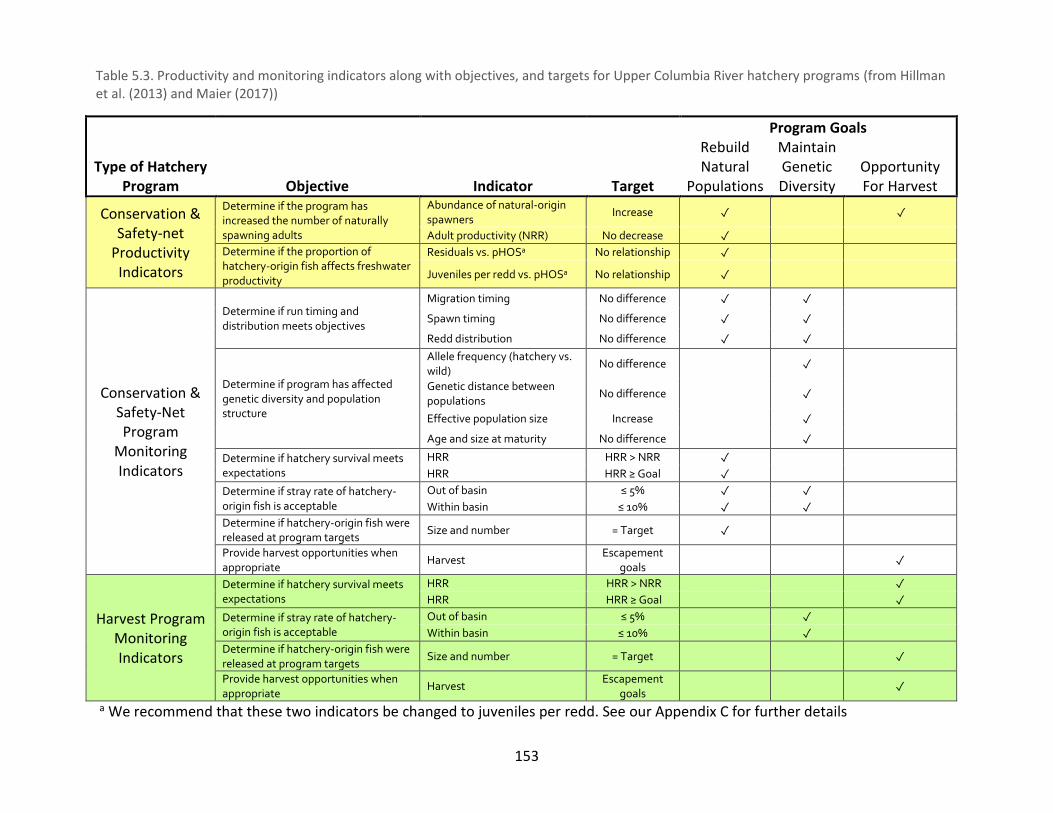
153
Table 5.3. Productivity and monitoring indicators along with objectives, and targets for Upper Columbia River hatchery programs (from Hillman et al. (2013) and Maier (2017))
Type of Hatchery Program
Objective
Indicator
Target
Program Goals Rebuild Natural
Populations
Maintain Genetic Diversity
Opportunity For Harvest
Conservation & Safety-net
Productivity Indicators
Determine if the program has increased the number of naturally spawning adults
Abundance of natural-origin spawners
Increase ✓ ✓
Adult productivity (NRR) No decrease ✓
Determine if the proportion of hatchery-origin fish affects freshwater productivity
Residuals vs. pHOSa No relationship ✓
Juveniles per redd vs. pHOSa No relationship ✓
Conservation & Safety-Net Program
Monitoring Indicators
Determine if run timing and distribution meets objectives
Migration timing No difference ✓ ✓ Spawn timing No difference ✓ ✓ Redd distribution No difference ✓ ✓
Determine if program has affected genetic diversity and population structure
Allele frequency (hatchery vs. wild)
No difference ✓
Genetic distance between populations
No difference ✓
Effective population size Increase ✓ Age and size at maturity No difference ✓
Determine if hatchery survival meets expectations
HRR HRR > NRR ✓
HRR HRR ≥ Goal ✓
Determine if stray rate of hatchery-origin fish is acceptable
Out of basin ≤ 5% ✓ ✓
Within basin ≤ 10% ✓ ✓
Determine if hatchery-origin fish were released at program targets
Size and number = Target ✓
Provide harvest opportunities when appropriate
Harvest Escapement
goals ✓
Harvest Program Monitoring Indicators
Determine if hatchery survival meets expectations
HRR HRR > NRR ✓
HRR HRR ≥ Goal ✓
Determine if stray rate of hatchery-origin fish is acceptable
Out of basin ≤ 5% ✓
Within basin ≤ 10% ✓
Determine if hatchery-origin fish were released at program targets
Size and number = Target ✓
Provide harvest opportunities when appropriate
Harvest Escapement
goals ✓
a We recommend that these two indicators be changed to juveniles per redd. See our Appendix C for further details

154
Metrics or indicators (see Table 5.3) used to evaluate harvest augmentation efforts differ from
those used to appraise conservation programs. The central goals of harvest programs are to
bolster fishing opportunities and segregate hatchery adults from natural spawning populations.
Consequently, performance indicators related to this type of program are quantification of
harvest opportunities, HOR recruitment rates, and stray rates. Regardless of whether a
hatchery program is based on conservation or harvest objectives both productivity and
monitoring indicators will be used for evaluation purposes (Hillman et al. 2017). Moreover, the
current plan is structured to allow direct assessments of management actions on monitoring
and productivity indicators. For instance, management decisions about the brood sources used
in hatcheries will influence monitoring indicators such as stray rates, run timing, and the
genetic properties of the supplemented populations. These in turn may affect, recruitment
rates of NORs, NOR abundance, and juveniles per redd which are considered productivity
measures.
The overarching goal of the hatchery-related M&E program is to identify empirical associations
between management decisions such as brood stock sources with productivity indicators like
NOR recruitment and abundance. The plan refers to these as “chain of causation” connections.
These connections between management actions and fish performance are used in the
program’s formal adaptive management process. If management actions are shown to be
ineffective or are preventing the program from achieving one or more of its primary goals, e.g.,
rebuilding natural populations, maintaining genetic diversity, or providing for harvest
opportunities, alternative actions are proposed, implemented, and subsequently evaluated.
A number of management strategies and M&E approaches have ensured that the effects of the
hatchery programs in the Upper Columbia are carefully appraised and adjusted when needed.
One notable management strategy was to create two committees (HCP Hatchery Committee
and Priest Rapids Coordinating Committee Hatchery Subcommittee) to provide oversight of
hatchery operations and production goals. Annual reporting of M&E results, establishment of a
five-year review process for the M&E program, the capacity to refine M&E methods in a
collaborative and transparent fashion, and the production of a well thought out adaptive
management process are other key management components. Additionally, the M&E program
is well crafted. It incorporates reference or control populations, predetermined statistical
analyses, along with an active and productive research program. In combination, these
elements permit effective changes to the M&E program as well as objective assessments of the
numerous Upper Columbia River hatchery programs.

155
5.4. Uncertainties Associated with Hatchery Fish Interactions in the Upper Columbia
5.4.1. Sufficiency of the Current M&E Program
The approaches and methods described in Murdoch et al. (2011) and Hillman et al (2017) are
generally appropriate to detect changes in fitness and abundance in the spring Chinook
populations undergoing supplementation. Upon review, we found areas where the methods
currently being used could be improved. These suggestions are provided in our Appendices C to
E. In section 5.4.3 below, several of these suggestions are briefly described.
5.4.2. Effect of Historical and Current Hatchery Programs on Fitness of the
Upper Columbia Spring Chinook ESU
This question has three parts. First, what is meant by fitness? Second what factors could be
used to determine whether fitness has been negatively or positively affected by historical or
current hatchery programs? Finally, what do the data and analyses produced by the RM&E
program and ancillary research tell us about how previous, and ongoing hatchery programs,
have influenced the fitness of individuals in the three extant spring Chinook populations in the
ESU? In a formal genetic sense, fitness measures the capacity of an individual to pass its genes
through time. It is typically measured by the number of adult offspring an individual genotype
produces relative to the contributions of other genotypes; the more offspring the greater an
individual’s fitness (Wilson 1975). In the above question, a broader definition of fitness is
implied. One based on the overall capacity of fish spawning in the same population to be self-
sustaining and thus capable of perpetuating their genes through time.
The M&E plan tracks temporal changes in abundance, productivity, spatial structure, and
genetic diversity (VSP parameters) relative to control or reference populations. Examination of
trends in these parameters is one way to ascertain if increases or decreases in fitness can be
associated with past and existing hatchery operations. A suite of factors, however, influences
VSP parameters. Environmental conditions experienced under artificial culture and genetic
changes due to domestication can affect age-at-maturation, sex ratios, size at maturity, choice
of spawning location, genetic diversity, and other traits. At the same time, environmental
conditions experienced by HOR and NOR adults and their offspring living in nature can also alter
VSP parameters. Disentangling the influences of these factors on VSP parameters has to occur
before long-term effects on fitness due to exposure to hatchery conditions can be estimated.
Life Cycle Models appear to be a promising way to tease out the effects caused by
contemporary hatchery programs. Estimates of the potential impacts of earlier fish cultural
practices are more problematic since they rely on historical accounts and speculations about
possible consequences.

156
5.4.2.1. Possible effects of historical fish culture activities on the fitness of Upper Columbia
River spring Chinook
Formerly robust populations of anadromous salmonids in the Upper Columbia had declined
substantially by the late 19th Century. Deteriorating conditions caused by agricultural practices,
mining, logging, the construction of impassable dams, unscreened irrigation diversions, and
overharvest prompted the Washington Department of Fish and Game to construct two
hatcheries, one in the Wenatchee subbasin and another in the Methow. Both were in operation
by 1899. The Wenatchee hatchery was located on Chiwaukum Creek about 40 miles upstream
from the Columbia River. This facility was closed in 1904 due to extreme weather conditions at
the site and difficulty in obtaining spring Chinook broodstock (Wahle and Pearson 1984). To
circumvent these difficulties a new hatchery was built near the town of Leavenworth,
approximately 25 miles upstream from the Columbia. It began operation in 1913 and was
abandoned in 1931. Collecting broodstock was difficult at this site and was probably one of the
reasons the hatchery was closed (Wahle and Pearson 1984).
The first Methow hatchery was located at the mouth of the Twisp River. Coho were an
important species cultured at the hatchery as approximately 12 million coho eggs were taken
from 1904 -1914. In 1915, an impassible dam was constructed near the mouth of the Methow
River. The hatchery was subsequently moved downstream from the dam, but the coho run was
strongly impacted. Egg takes from this species declined, and no coho eggs were obtained after
1920. The hatchery continued to operate until 1931, incubating eggs and releasing steelhead,
Chinook, and chum salmon fry obtained from other river sources (Wahle and Pearson 1984).
Survival rates of fish produced from these early hatcheries undoubtedly were low. Hatchery fish
were typically released as fry, eggs from outside stocks were commonly imported which further
reduced potential survival, and little research on improving salmon culture methods was
performed during the early 20th century. Consequently, few (if any) hatchery origin adults were
presumably produced and available to interbreed with NORs. However, acquisition of native
broodstock to support these programs could have reduced spatial structure, genetic diversity,
and overall abundance of anadromous fishes returning to the Wenatchee and Methow
subbasins. Information on when and where broodstock were collected, proportion of the
population that was removed, and actual number taken are needed to evaluate the full impact
of broodstock mining. Blankenship et al. (2007) report that the Leavenworth state hatchery
used eggs from non-native stocks (Willamette River spring Chinook and lower Columbia River
hatchery fall Chinook), suggesting that problems with obtaining adequate numbers of
broodstock were prevalent. Perhaps the physical challenges (e.g., freshets, weir maintenance,
etc.) faced by early fish culturists reduced the number of adults they could obtain. This, and
their reliance on out-of-basin stocks, would have limited the impacts of their collection efforts
on native salmonids. Alternatively, local abundances could have been so low it made obtaining

157
broodstock difficult. In the latter situation, removal of NORs could substantially alter VSP
parameters.
In 1939, Grand Coulee Dam blocked anadromous fish from using ancestral spawning and
rearing areas in more than 1,000 linear river miles (Fish and Hanavan 1948). To mitigate for this
loss, a second phase of hatchery construction and use began under the Grand Coulee Fish
Maintenance Project (GCFMP). A detailed account of the accomplishments and setbacks of the
first nine years of the GCFMP can be found in Fish and Hanavan (1948). They report that natural
salmon runs in the Wenatchee, Entiat, Methow, and Okanogan subbasins had been
“decimated” over the previous 30 to 40 years. Efforts were underway in the 1930s to remove or
place fishways on impassable dams and to install screening on major irrigation ditches. Because
of these improvements and scarcity of natural fish, it was determined that Upper Columbia
subbasins would be appropriate locations for translocating adult salmonids destined for natal
areas upstream of the Grand Coulee Dam.
Adult salmon were captured at Rock Island Dam from 1939 – 1943. Originally, these fish were
supposed to be transported to holding areas in Icicle Creek and used for broodstock at a central
hatchery located at Leavenworth. Neither the Leavenworth hatchery nor any of its proposed
sub-hatcheries intended for the Entiat, Methow, and Okanogan were completed in time to
receive fish in 1939. Adult salmon were instead hauled and released into enclosed areas in the
Wenatchee, Entiat, and Okanogan Rivers. For example, in the Wenatchee River, spring Chinook
and steelhead were placed into the lower 16 miles of Nason Creek. Additionally, summer
Chinook were placed into an 18-mile portion of the river located below Lake Wenatchee, and
sockeye were also introduced into Lake Wenatchee. Summer Chinook and steelhead were
placed into a 15-mile stretch of the Entiat River, and additional sockeye were transported to
Lake Osoyoos in the Okanogan subbasin. Approximately 100 linear miles of stream were
impounded and used for natural production. Routine inspections of these areas showed that
fish were successfully spawning. This led the GCFMP to continue to release adults into these
locations until 1944 when adults were no longer intercepted at Rock Island Dam (Table 5.4).

158
Table 5.4. The number and spawning success of spring and summer Chinook transplanted into the Wenatchee River from 1939-1943. Data from Fish and Hanavan (1948).
Year
Race of Chinook
Location
Number Released
Number of Carcasses Sampled
% Spawned
1939
Spring Nason Creek
3,957 423 77 1940 3,165 574 67 1941 1,251 417 37 1942 1,014 255 51 1943 1,191 243 86
1939
Summer Upper Wenatchee
3,498 1,052 83 1940 752 169 93 1941 446 94 60 1942 3,050 776 39 1943 386 No Dataa No Dataa
a flooding destroyed the rack in the upper Wenatchee in 1943, no sampling occurred
By 1940, the Leavenworth Hatchery and its satellite hatcheries in the Entiat and Methow were
ready to receive fish. From 1940 – 1943, adult spring and summer Chinook collected at Rock
Island Dam were used as broodstock at the Leavenworth Hatchery. Additionally, from 1940 –
1947 eyed Chinook salmon eggs from the McKenzie River, Big White Salmon River, Spring
Creek, and from the Wind River (Carson Hatchery) were imported into the hatchery (Fish and
Hanavan 1948). Initially Chinook eggs from these various sources were also shipped from the
Leavenworth Hatchery into the Entiat and Methow hatcheries for further incubation, rearing,
and release. That practice stopped once the value of using locally adapted fish for broodstock
was recognized. Sporadic importation of Chinook eggs from Lower River Chinook populations,
however, continued at Leavenworth until 1985 (Potter 2016). Although spring Chinook have
been produced at Leavenworth since 1940, sockeye were the main species raised at the
hatchery. By the early 1970s the sockeye program was terminated due to disease concerns
(Potter 2016). From this point on, Chinook became the principal species cultured at
Leavenworth. Currently, they are being used in a segregated harvest augmentation program.
The overall effect of the Grand Coulee Fish Maintenance Project on the fitness of Upper
Columbia River Chinook populations can be hypothesized if the project is regarded as a large
salmonid transplant effort. The results of past attempts to transplant salmonids were
summarized by Withler (1982) who observed,
“Transplants within the Pacific salmons’ normal range have been singularly
unsuccessful in producing new anadromous stocks, except where natural
colonization has been prevented by an obvious physical barrier. In only one of

159
many transplants into watersheds where there was no physical obstruction to
upstream migration has a new run developed: sockeye fry and fingerlings of
Skagit River origin planted in 1937 in Issaquah Creek (Lake Sammamish) and
Cedar River (Lake Washington) developed into self-perpetuating runs.”
Quinn (2005) offers a possible explanation for why such actions persistently end in failure by
hypothesizing that accessible habitat in the areas being colonized are already fully occupied.
The source of the fish being transplanted is also critical. Return rates of adult coho from 13
paired releases of local and non-local hatchery fish showed that there was an exponential
decline in recovery rates with transfer distance. The farther away a non-local stock was from its
natal location, the poorer its recovery rate was (Reisenbichler 1988; Quinn 2005). Mismatches
with other factors associated with local adaptation (e.g., resistance to parasites and diseases,
migration and reproductive timing, energy reserves at the adult stage, egg size, size and age at
maturity, adult morphology, seawater entry date, etc.) may have contributed to transplant
failures.
The extensive history of past transplant failures cast doubts on whether the GCFMP successfully
preserved any of the genetic heritage of the salmonid stocks located above Grand Coulee Dam.
Small extant populations of salmonids existed in Upper Columbia prior to the GCFMP (Fish and
Hanavan 1948). It is possible that these fish had fully seeded the poor juvenile habitat then
available. Additionally, the spring and summer Chinook captured at Rock Island Dam and used
as hatchery broodstock or natural spawners, originated from multiple upstream spawning
areas. Fish obtained from distant upstream populations would probably fare worse than those
originating from populations closer to their transplant locations (Reisenbichler 1988),
potentially reducing genetic diversity substantially.
On the other hand, under some circumstances, transplants of Chinook salmon within their
native range have created self-sustaining populations. In their review of previous transplant
attempts, Fedorenko and Shepherd (1986) identified a number of factors that led to successful
transplants. The most important factors were close ties to a hatchery program that provided
annual releases of one million or more juveniles, program persistence of a decade or more, use
of three or more donor populations and hybrids among the donor stocks, extensive juvenile
rearing and acclimation at release locations, and the production of relatively large and healthy
juveniles. Overall, the GCFMP program and its subsequent hatchery program met these
requirements. But other requirements identified by Fedorenko and Shepherd may not have
been met (i.e., use of geographically close donor stocks (<100 km) with similar freshwater
migratory routes, presence of suitable spawning and rearing areas, adequate forage base).
Currently, it is unknown if any of the genetic legacy contained in the salmonid populations
native to areas above Grand Coulee Dam was retained. This question could be resolved if scale

160
samples from adults used as broodstock at Leavenworth and its satellite hatcheries during
1940-1943 were taken and are still available. Procedures now make it possible to extract DNA
from scales, and genetic signatures from these historic samples could be compared to those
obtained from contemporary spring and summer Chinook salmon in the Upper Columbia.
Beginning in the 1960s, additional efforts were initiated to mitigate for habitat losses due to the
construction and operation of the five mid-Columbia River PUD dams. Three hatcheries were
established: Chelan, Columbia Basin, and Wells. Possible effects of the Columbia Basin and
Chelan hatcheries are not considered here since Chinook are not cultured at either of these
facilities. Along with hatchery construction, spawning channels for summer/fall Chinook were
also built in the vicinity of Priest Rapids (1963), Rocky Reach (1961), and Wells (1967) dams. The
channels were operated for just a few years before it was decided that they were not
functioning as designed. A hatchery facility was subsequently built at Priest Rapids and portions
of its spawning channel are now being used for fish rearing purposes. Similarly, the Turtle Rock
spawning channel (Rocky Reach) was converted into a rearing facility for juvenile salmonids.
The Wells spawning channel was removed during a recent renovation of the Wells Hatchery. In
the late 1980s and early 1990s, the Eastbank Hatchery with five satellite facilities and the
Methow Hatchery with two satellite ponds were constructed (SRT 1998-33). Potential effects of
these newer hatcheries on the fitness of NOR spring Chinook in the Upper Columbia are
discussed below.
5.4.2.2. Possible effects of current fish culture activities on VSP parameters (fitness) of Upper
Columbia River spring Chinook
Ongoing Monitoring and Evaluation in the Upper Columbia is designed to assess how hatchery
operations may affect VSP parameters. Murdoch et al. (2011) and Hillman et al. (2017)
presented results on responses of VSP parameters to supplementation for Methow and
Wenatchee spring Chinook populations, respectively. Besides these assessments, research in
the UCR included: (a) the validity of using redd counts and carcass data to estimate population
abundance (Murdoch et al. 2010), (b) the relative reproductive success of HOR and NORs
spawning in nature (Williamson et al. 2010), (c) factors responsible for differences in
reproductive success (Hughes and Murdoch 2017), (d) the reproductive success of hatchery-
origin precocious parr (Ford et al. 2015), and (e) stray rates of HOR and NOR adults (Ford et al.
2015). These studies provided additional insights into how supplementation may be affecting
VSP parameters in Upper Columbia spring Chinook.
The M&E plan (see Table 5.3) prioritizes two VSP parameters, abundance (NOR and total) and
productivity. These parameters are evaluated in supplemented populations by comparing them
to values and trends in reference populations. Hillman et al. (2017) emphasized that abundance
and productivity are rarely measured in the field. Instead, other indicators (e.g., redd counts,

161
fish counts at weirs, scales, tags, etc.) are used to estimate them. Those estimates often rely on
assumptions (e.g., fish/redd, pre-spawning loss, marking rates, etc.), which increases their
variability (Hillman et al. 2017). Consequently, if disparities are detected, they likely are
substantial because the elevated variation in the parameters being compared reduces the
power to detect differences. Also, as described above (5.4.2.1), spring Chinook populations in
the Upper Columbia have been exposed to a long history of hatchery transplants and
supplementation. Potentially, many NORs and HORs could share the same hatchery ancestors,
potentially narrowing genetic differences between them. It also enhances the possibility that
the origin of observed divergences is due to environmental differences between hatchery and
natural environments rather than by genetic changes.
In the Methow, three spring Chinook supplementation efforts located on the Twisp, Chewuch,
and Methow Rivers were evaluated by Murdoch et al. (2011). Supplementation began in 1992
and has been modified since its inception. In its current configuration, a composite broodstock
of Chewuch and Methow adults, is used for the Methow and Chewuch programs. Broodstock
for the Twisp program is obtained from the Twisp River. All the eggs for these programs are
incubated at the Methow Hatchery. Methow juveniles are released into the Methow River
while those designated for the Chewuch and Twisp are transported to their rivers for final
acclimation and rearing. In the early years (1992 - 1999) of the Methow supplementation
project, the National Fish Hatchery at Winthrop reared and released “Carson” stock spring
Chinook as part of a segregated harvest augmentation program. In 2000, the Winthrop
Hatchery switched to using local broodstock. At present, spring Chinook adults (F1) produced
by the Methow supplementation program are used as broodstock at the Winthrop Hatchery as
part of a safety net program.
Results of some of the comparisons performed by Murdoch et al. (2011) are summarized in
Table 5.5. They show that the overall abundance of spring Chinook in the three populations did
not increase relative to reference populations. At the same time, supplementation did not
affect productivity. Additionally, NOR abundance in the Chewuch and Methow did not change
although it decreased in the Twisp. These results differ somewhat from those obtained from an
evaluation of a spring Chinook supplementation program in the Imnaha River. Like the Methow
programs, NORs in the Imnaha did not increase due to supplementation. But the overall
abundance of spring Chinook in the Imnaha did increase and productivity decreased. Reduced
productivity in the Imnaha was linked to differences in spawning locations, spawn timing, and
decreases in age- and size-at-maturation in hatchery fish (orafs.org/wp-
content/uploads/2015/03/ Session-2-5-Hoffnagle.pdf). In contrast, NORs and HORs spawned at
similar times and places in the Methow. Additionally, no differences in size were detected when
age and sex were held constant. These similarities were likely responsible for the maintenance
of productivity in the supplemented Methow populations.

162
In the Wenatchee subbasin, there are three spring Chinook hatchery programs. Two of these
are conservation efforts, located at the Chiwawa River and nearby at Nason Creek. A
segregated harvest augmentation endeavor located at the Leavenworth Hatchery is the third
hatchery program. The M&E plan (Murdoch et al. 2011, Hillman et al. 2017) contains a
comprehensive account of the analytical steps and procedures being used to evaluate the
ecological and genetic effects of the conservation programs on NOR spring Chinook in the
Wenatchee River. An evaluation of the Chiwawa supplementation program is included in the
M&E plan to illustrate how the proposed analytical methods should be applied.
Supplementation influences on overall adult abundance (NORs + HORs), NOR abundance, and
productivity in the Chiwawa were investigated. Multiple steps were taken to select appropriate
reference populations that could act as controls in the analyses. After the reference
populations were selected, analyses using trends, mean differences, ratios, rates, and spawner
recruit models were used in the evaluation process. Additional steps were also undertaken to
account for possible density-dependent and carrying capacity effects (Hillman et al. 2017). This
approach meant that multiple independent analyses were used to examine the same effects of
the Chiwawa project.
The principal results of these different analyses were quite similar. There was no evidence that
the supplementation program in the Chiwawa increased overall abundance or the abundance
of NORs.

163
Table 5.5. Summary of some of the assessments made on NOR and HOR spring Chinook originating from the Methow, Chewuch, and Twisp supplementation programs. Abundance and productivity assessments are made relative to what occurred in reference streams. Other comparisons are based on observations made on fish returning to the Methow. Data from Murdoch et al. (2011)
Supplementation Program
Parameter
Finding
Twisp Overall Abundance Declined relative to reference populations Chewuch Overall Abundance No evidence of an increase Methow Overall Abundance No evidence of an increase Twisp NOR Abundance No evidence of a change Chewuch NOR Abundance Declined relative to reference populations Methow NOR Abundance No evidence of a change Twisp Productivity No evidence of a change Chewuch Productivity No evidence of a change Methow Productivity No evidence of change Twisp Redd Distribution NORs & HORs have similar distributions Chewuch Redd Distribution NORs & HORs have similar distributions Methow Redd Distribution Lower downstream sites by HORs in some yrs. Twisp Mean Brood year Stray
Rate 36% -mainly within the Methow subbasin
Chewuch Mean Brood year Stray Rate
39% -mainly within the Methow subbasin
Methow Mean Brood year Stray Rate
3%
Twisp Age At Maturity No differences found Chewuch Age At Maturity NOR & HOR females no difference; HOR males
younger Methow Age At Maturity NOR & HOR females no difference; HOR males
younger Twisp Size At Maturity Within a sex: 4-yr-old HORs & NORs were similar
in size Chewuch Size At Maturity Within a sex: 4-yr-old HORs & NORs were similar
in size Methow Size At Maturity Within a sex: 4-yr-old HORs & NORs were similar
in size

164
Twisp Genetic Diversity Remain distinct from other spring Chinook in Methow
Chewuch Genetic Diversity Decreasing over time, closely related to Methow stock
Methow Genetic Diversity Closely related to Winthrop and Chewuch stocks Twisp Effective Population Size Ratio of Ne/N remains constant as expected Chewuch Effective Population Size Ratio of Ne/N remains constant as expected Methow Effective Population Size Ratio of Ne/N declined and is not related to
abundance
As in the Methow, there was no evidence that productivity was affected by supplementation. A
non-significant negative trend was found between increasing levels of pHOS and productivity;
suggesting that HORs may not be as productive as NORs. After carrying out their exhaustive
evaluations, however, the authors state, “based on these analyses, there is no strong evidence
that the supplementation program has significantly benefited or harmed the natural spring
Chinook population” (Hillman et al. 2017).
Before concluding that the current supplementation efforts are not appreciably influencing VSP
parameters in NOR populations three other issues need to be briefly discussed. First, straying
rates in some hatchery programs are quite high. For example, HORs produced by the Chewuch
and Twisp projects were found to have stray rates greater than 35% (Table 5.6). It was noted,
that many of these fish were recovered at the Methow Hatchery, the location where they were
incubated and reared for a period of time. Few strayed into other Upper Columbia River
subbasins (Murdoch et al. 2011). Nevertheless, concerns were raised about how straying and
hatchery operations may be reducing genetic diversity among Methow subbasin spring Chinook
stocks. For instance, the genetic diversity of the Chewuch population is decreasing and
becoming similar to the Methow. This may be due to straying. Significant straying (37%) has
also been observed in HORs produced by the Chiwawa program. Clearly, some degree of
straying is beneficial as it may expand the spatial diversity of a population. Excessive straying
however, has the potential to erode stock specific adaptations and lead to lower productivity
(Ford et al. 2015).

165
Table 5.6 Average stray rates by brood year in spring Chinook salmon produced by Upper Columbia River hatchery programs. Percentage values equal the proportion of the fish that were not detected in target watersheds. In-basin and out-of-basin straying is included in the percentage value. Data are from the Upper Columbia Salmon Recovery Board; Hillman et al. 2016; Snow et al. 2016; Humling et al. 2016; and Cooper et al. 2017.
Spring Chinook Hatchery Program
Brood Years Evaluated Average Brood Year Stray Rate
Chiwawa Brood Years 2005 -2009 37% Methow Brood Years 2005 -2009 3% Twisp Brood Years 2005 -2009 36% Chewuch Brood Years 2005 -2009 39% Winthrop Brood Years 2005 -2009 36.5% Leavenworth Brood Years 2005 -2009 4%
Research conducted on the Wenatchee River using parentage analysis compared straying
tendencies in NORs and HORs (Ford et al. 2015). Results produced by this study raised a
number of important questions about the roles of habitat quality, parental origins in naturally
spawning fish, and possible genetic changes caused by hatchery conditions on the proclivity to
stray. More of this work should be performed to provide additional insights into the factors that
induce straying and on how it may be reduced. Dittman et al. (2015) recount that laboratory
and field studies indicate that embryonic imprinting on natal waters occurs in salmonids from
hatching to emergence. They hypothesize that straying could be reduced or that HORs could be
directed to spawning sites by exposing salmonid alevins to artificial odors or to waters from
desired spawning locations while the fish are incubating in a hatchery environment. This idea
capitalizes on the fact that adult salmon sequentially follow a set of stream odors to natal
spawning areas, moving upstream until they reach sites with odors that were imprinted upon at
the embryonic stage. In theory, HORs returning to a centralized incubation hatchery (e.g.,
Methow) could be guided to targeted spawning areas by using additional upstream olfactory
cues. We hope that a pilot study examining this possibility can be undertaken in the future,
perhaps in one of the Upper Columbia spring Chinook hatchery programs.
Second, the tendency for hatchery conditions to induce precocious maturation in spring
Chinook also may affect VSP parameters in supplemented populations. In some circumstances,
precocious maturation rates of hatchery males can be greater than 90% (Shearer et al. 2006;
Larsen et al. 2004, 2013; Harstad et al. 2014; Don Larsen pers. comm.), an order of magnitude
greater than such rates in nature (Larsen et al. 2013). Consequently, large numbers of
precocious males can be released from hatchery programs. Not much is known about their
capacity to reproduce in nature. Recently, Ford et al. (2015) used parentage analysis to evaluate
the breeding success of hatchery origin precocious parr in the White River. Anadromous males

166
produced about five times as many offspring per spawner as precocious parr. Nevertheless,
approximately 33% of the progeny produced were apparently fathered by precocious males
because of the large number of precocious males in the spawning population (Ford et al. 2015).
Possible causes (e.g., genetic, epigenetic, environmental, and genetic x environmental
interactions) of early maturation in hatchery fish are not completely known (Ford et al. 2015).
Ford et al. (2015) discussed some possible repercussions of early maturation. If early
maturation has a genetic origin, successful reproduction could be of concern because the
genotypes present in precocious parr may not be representative of those that would have
existed if the fish had experienced a typical anadromous life cycle. If on the other hand,
maturity is largely a response to rearing conditions, early maturing males would likely not
contribute deleterious genetic changes to supplemented populations. Additionally, Ford et al.
(2015) suggest:
“If early maturity is the result of genotype x environmental interactions such that
some genotypes that would not have matured early in the wild do mature early
when reared in the hatchery, then successful reproduction by early maturing fish
may in fact even be necessary to avoid genetic changes due to hatchery rearing.”
Studies to evaluate the factors responsible for early maturity in hatchery fish are needed before
the conservation implications of this phenomenon can be fully understood.
Third, three assessments were performed that examined possible genetic changes caused by
the supplementation programs that started in the early 1990s. Two of those efforts were
focused on spring Chinook. One compared genetic samples obtained from Methow spring
Chinook prior to supplementation (1992-93) to those obtained up to 2006 (Small et al. 2007).
Samples came from the Winthrop National Fish Hatchery (WNFH) and from natural and
hatchery fish collected in the Methow, Twisp, and Chewuch Rivers. Spring Chinook from the
Twisp Hatchery and Twisp River were genetically differentiated from the Methow-Chewuch
group. The Methow population was closely related to the Carson stock, the out-of-basin stock
that was used at the WNFH until 2001. Additionally, the Methow and Chewuch populations
became more similar over time because of a change in how broodstock was acquired for those
programs. Beginning in 2001, adults obtained from the Methow and Chewuch River were
aggregated to form a single broodstock. Other than this change, no significant differences
between pre- and post-supplementation periods were found. Genetic diversity measures
(heterozygosity and allelic richness) were unchanged and the Twisp population still remained
differentiated from the Methow-Chewuch group. Temporal changes in effective population size
(Ne) were not detected and appear to be stable in the Methow and Chewuch populations.
However, Ne is declining in the Twisp population and is precipitously low. This decline has been
slowed somewhat by supplementation. Also, Small et al. (2007) note that strays from the

167
Methow-Chewuch population are entering the Twisp and are likely reducing differentiation
among the three populations.
A similar evaluation was undertaken on spring Chinook returning to the Chiwawa River
(Blankenship et al. 2007). As with the Small et al. (2007) study, genetic samples obtained pre-
and post-supplementation were analyzed and compared. Post-supplementation census size
was similar to what it had been prior to supplementation. Additionally, the genetic diversity of
NORs appeared to be unaffected by supplementation, hetrozygosities are high, and
contemporary Ne is similar or perhaps slightly higher than it was before supplementation
(Blankenship et al. 2007). There was slight but statistically significant differentiation among
spring Chinook in the Chiwawa River, White River, and Nason Creek. Yet, 99.3% of the genetic
variation observed was within samples, and very little could be linked to population differences
(Blankenship et al. 2007). This was probably caused by large amounts of gene flow among these
populations or by very recent divergence (Blankenship et al. 2007).
A final genetic assessment examined the population structure of Upper Columbia summer
Chinook from the Wenatchee, Methow, and Okanogan Rivers (Kassler et al. 2011) to determine
if supplementation had impacted the genetic structure of these populations. Population
differentiation among these populations was not observed in any of the pre- or post-
supplementation samples. This suggests that genetic homogenization or extensive gene flow
among these populations occurred prior to contemporary supplementation. Pairwise FST
comparisons between the summer Chinook populations and eight fall Chinook and two summer
Chinook populations (Entiat and Chelan River) were also performed. FST values were less than
0.01 for summers vs. falls from Hanford Reach, Lower Yakima, Priest Rapids, and Umatilla.
These low FST values probably occurred because in the 1970s and 80s fall Chinook were
commonly spawned with Upper River summer Chinook. This created a single homogenized
summer/fall population. There was also very little evidence of differentiation between the
Chelan River and Entiat populations and summer Chinook returning to the Wenatchee,
Methow, and Okanogan. No change in Ne from the 1993 to 2008 was found. Kassler et al.
(2011) conclude their assessment by stating that the genetic diversity of summer Chinook in the
Upper Columbia has not been altered by the ongoing supplementation program.
In summary, the spring Chinook supplementation program that began in the 1990s in the
Methow has decreased genetic differentiation among the Methow, Chewuch, and Twisp
populations. On the other hand, genetic diversity and effective population sizes have been
largely maintained in these populations. Similarly, genetic diversity and Ne values have not been
affected by supplementation in the Chiwawa River. Unlike the Methow, however, the spring
Chinook populations in the Wenatchee (Chiwawa and White Rivers and Nason Creek) appear to
have been homogenized prior to the current supplementation effort. Genetic analyses of Upper

168
River summer Chinook also indicate that summer Chinook passing over Rock Island Dam
originate from one homogenized population, created by the artificial mixing of endemic
summer and fall run fish. As with the other two genetic assessments, contemporary
supplementation has maintained Ne and genetic diversity in Upper Columbia summer Chinook.
Consequently, it appears that historical events prior to the current supplementation efforts
were largely responsible for decreasing genetic diversity and homogenizing Upper Columbia
spring, summer and fall Chinook.
The supposition that Upper Columbia spring Chinook have lost a substantial amount of their
past genetic diversity was recently supported by genetic analyses (Johnson et al. 2018). They
compared mitochondrial DNA (mtDNA) haplotype richness, haplotype and nucleotide diversity,
and population differentiation among ancient Upper Columbia and Snake River Chinook to
contemporary Chinook populations in the Upper Columbia and Snake subbasins. Compared to
their ancestral predecessors, Chinook in both the Upper Columbia and Snake subbasins have
lost genetic diversity. Chinook from the Upper Columbia experienced greater genetic losses
than those returning to the Snake subbasin. Haplotype and nucleotide diversity in
contemporary Upper Columbia Chinook were about 1/3rd of their ancestral values.
Alternatively, present day Chinook from the Snake subbasin retained about 2/3rds of their
ancestral haplotype and nucleotide diversity. Haplotype richness (presence and proportion of
haplotypes) in the Upper Columbia subbasin has also decreased. Loss of genetic diversity
experienced by Upper Columbia Chinook theoretically reduces their capacity to respond to new
selection pressures; e.g., to climate change and its associated effects on water temperatures,
flow regimes, and dynamic weather events.
The results obtained by Johnson et al. (2018) came from a relatively small collection of ancient
samples. They nevertheless suggest that a substantial amount of genetic diversity has been lost.
Some still remains though. Five matriarchal haplotype lineages still exist in Upper Columbia
Chinook salmon, and managers are aware of the benefits of using local stocks in conservation,
safety-net, and harvest augmentation programs. So far, current hatchery operations have not
increased overall abundance or the abundance of NORs. At the same time, productivity of these
populations appears to be stable. The current M&E plan provides information for researchers
and managers to use in an adaptive management program. It is hoped that ongoing
management practices will maintain current levels of genetic diversity and that natural
selection will be allowed to once again act as a creative agent, yielding additional genetic
differentiation and population structure in Upper Columbia Chinook.
5.4.3. Recommendations
The ISAB recommends that the UCSRB consider the design of their overall RME program for all
Hs in their future efforts to develop a systematic, collective process for coordination of the
169
actions, monitoring efforts, and decisions across the numerous working groups and
coordinating committees in the three subbasins (see Recommendations in Chapter 4). The RME
program is funded largely through the responsibilities of the PUDs under licensing agreements.
As a result, it is largely focused on assessing hatchery practices and the effects of hatcheries on
spring Chinook salmon populations. While this is a critical aspect of recovery in the Upper
Columbia, it does not address all actions of the recovery program. Currently, there is no RME
Plan that encompasses all Hs and their related working groups, and there is no process to
coordinate monitoring efforts across the subbasins and address information needs related to all
Hs.
Approaches and methods of the RTT, PUDs, and regional fisheries agencies are generally
appropriate and can be used to answer questions about effects of hatcheries and the
hydrosystem, but analyses could be improved. Upper Columbia RME planning efforts among
the PUDs, WDFW, UCSRB resulted in a thoughtful process to identify reference populations that
could be utilized to help assess how hatchery supplementation efforts were influencing total
spawner abundance, natural origin spawner abundance, and productivity (recruits per spawner)
in supplemented streams.
In many instances in the Upper Columbia, the RME program compares a supplemented
population to three or more reference populations, but the results of the individual
assessments are not aggregated. A more sophisticated analytical approach that simultaneously
examines data from the supplemented population and all reference populations would improve
the precision of the estimates and increase the power to detect effects.
The RME efforts track temporal changes in abundance, productivity, spatial structure, and
genetic diversity (VSP parameters) relative to control or reference populations. However, many
factors (e.g., environmental conditions experienced under artificial culture, genetic changes due
to domestication, environmental conditions experienced by adults and their offspring in natural
streams) can also alter VSP parameters. Influences of these factors on VSP parameters must be
disentangled before long-term effects of hatchery practices on fitness can be estimated. Life-
cycle models are a promising way to evaluate the relative effects of ecological concerns and
human actions to better design and prioritize information needs and potential effectiveness of
restoration actions.
Assessing potential impacts of early fish cultural practices is problematic because they rely on
historical accounts and speculations about possible consequences. Recent genetic studies of
Columbia River Chinook indicate hatchery practices and effects of mainstem and tributary dams
have reduced genetic diversity of Upper Columbia spring Chinook populations. Genetic analyses
offer increasing potential to quantify the influences of past practices on the fitness of
anadromous salmon and steelhead populations.

170
Throughout this chapter we identified analytical methods that Upper Columbia managers and
researchers may wish to consider. Greater detail and more comprehensive discussions on
recommended statistical approaches can be found in our Appendices C to E.
Statistical and Analytical Suggestions
1. When comparing the migration timing, spawn timing, and redd distributions of NOR and
HORs spawning in nature, we recommend the use of Kolmogorov-Smirnov Two-Sample
Tests (K-S test). K-S tests are used to compare two frequency distributions, e.g., the
distribution of NOR and HOR redds throughout a stream basin, or timing differences by
Julian dates in migration and spawning. These tests are sensitive to a variety of
differences that may exist in the two distributions being compared, not just central
location (means) but also to skewness, dispersion, etc. (Siegel 1956).
2. Measures of uncertainty (e.g., standard errors) need to be calculated for stray rates. The
methodology for estimating stray rates for Chinook based on CWT expansions for
tagging proportions and catch searched is appropriate. Yet, standard errors are needed
to help put calculated rates into perspective. Currently, it is unclear if a 17% stray rate
has an uncertainty of ± 1% or ± 15%.
3. The process used to select reference populations employed both statistical (e.g.,
presence of a long-time series in abundance and productivity estimates, harvest
estimates, etc.) and biological (similar life history traits, few or no hatchery fish, similar
trends in freshwater habitat, etc.) criteria. Statistical criteria have little bearing on the
suitability of a reference stream. All else being equal, biological criteria should be given
more weight when selecting reference populations.
4. At present, separate analyses are being used to compare treated (supplemented)
populations with a single reference population. Often, treated populations are
compared to three or more suitable reference populations. The results of these
comparisons, however, are never aggregated. We recommend that data from a
treatment population and all of its reference populations be compared simultaneously.
This will lead to improved precision and also increase the power to detect differences.
Such models can be fit using standard software (e.g., R). However, we recommend that
a Bayesian Analysis be used. It will allow the incorporation of prior beliefs on the value
of supplementation, integration of multiple performance measures, and can more easily
deal with unequal variances in the different populations.
5. Differences between treatment and reference populations are quantified by using ratio
scores. These were calculated by dividing values from the treatment population by
those from a reference population. The authors recommend that these ratios be

171
analyzed using original values. However, many biological effects are multiplicative
rather than additive. To account for multiplicative effects the log(T/R) should be used
rather than arithmetic values.
6. The M&E Plan makes extensive use of null hypothesis statistical testing to evaluate the
impact of hatchery supplementation efforts in the Upper Columbia. These tests are
being used to detect both positive and adverse effects. Null hypothesis testing is not
really designed to assess “no impact” hypotheses. Given a large enough sample size, it is
almost certain that that some effect will be detected, but it may not be biologically
relevant. To directly assess a “no impact” hypothesis, a modification to the Null
Hypothesis Statistical Test framework may be useful, namely Equivalence Testing Refer
to (en.wikipedia.org/wiki/Equivalence_test) and our Appendix C for further details.
7. The greatest disadvantage of the Null Hypothesis approach is that it does not provide a
direct answer to the question—how certain is it that supplementation has an effect or
not had an effect? The p-value does not serve this purpose. The p-value measures the
consistency of the data with no effect, which can be easily misinterpreted. We think a
Bayesian approach may be more useful. The posterior belief about a parameter provides
a direct interpretation on the question of interest. For example, consider again the
productivity indicator of abundance of natural spawners (first row of Table 1 in Hillman
et al. 2017). Under the NHST framework, a p-value of 0.02 indicates that the observed
data is not consistent with no effect—hardly an interpretation that can be interpreted
with ease. Under a Bayesian framework, a posterior belief of 0.98 that the mean
abundance has increased under supplementation is easily interpreted. For most of the
analyses proposed in the M&E plan a Bayesian analysis is easily implemented.
Suggestions for Additional Research
1. Outputs from the PCD-Risk_1 Model that was used to evaluate potential interactions
between hatchery fish and non-target-taxa of concern (NTTOC) in the Upper Columbia
are hypotheses or expected outcomes. We recommend that existing data be used to
validate some of the outcomes produced by the model. Results from such analyses
would be of real interest to NOAA-Fisheries and others that are using the model to
examine possible hatchery fish x NTTOC interactions in the Basin. Ideally, field sampling
similar to that occurring in the Upper Yakima River could also be started in selected
areas in the Upper Columbia. Data from such efforts could be used to further test the
accuracy of the initial PCD-Risk_1 Model outputs.
2. Continued development and validation of the life-cycle model being developed for
Wenatchee River spring Chinook is encouraged. The model is designed to evaluate the

172
effects of hatchery domestication, climate change, pinniped predation, ocean
conditions, and freshwater habitat on the population dynamics of Wenatchee spring
Chinook. At present, many of the model’s parameter values are fixed with only a few
being estimated by an ad hoc calibration method. Given its many assumptions and fixed
parameters its current outputs can only be used qualitatively (ISAB 2017-1). The model,
however, appears to have the flexibility to incorporate new data, and efforts to refine it
are underway. When completed, it has the potential to be a valuable tool for
management.
3. It is unknown if any of the genetic legacy from Chinook stocks native to areas of the
Columbia River above the Grand Coulee Dam were retained by the Grand Coulee Fish
Maintenance Project. There may be one possible way to resolve this question. If scales
were collected on the spring Chinook spawned at Leavenworth from 1940 – 1943, and if
they are still available, it should be possible to extract DNA from these samples. Results
from these analyses could be compared to the genetic profiles that exist on spring
Chinook currently in the Upper Basin.
4. Dittman et al. (2015) have proposed that hatchery fish can be directed to targeted
spawning locations if they are exposed to artificial odors or to waters from desired
spawning locations from hatching to yolk absorption. We encourage Upper Columbia
researchers to continue working with Dittman and colleagues and implement a pilot
project to test the feasibility of this approach. It has the potential to greatly reduce
straying and possibly eliminate the need for expensive acclimation sites.
5. Further Investigations that explore the factors responsible for early maturation in male
spring Chinook salmon are also encouraged. Ford et al. (2015) indicates that the
conservation benefits and risks associated with releasing precocious parr are affected by
the factors that drive early maturation in hatchery stocks. Consequently, a thorough
understanding of what enhances precocious maturation in hatchery stocks would help
determine if anything should be done to control the release of early maturing male parr.
173
6. Modeling
6.1. Specific Comments about Life-Cycle Models
There are four life-cycle models developed for the Upper Columbia ESU (Table 6.1). All of these
life-cycle models are based on a standard life-cycle formulation with different emphases at
different life stages. For example, the Methow River model uses a food web at the juvenile
stage; the Wenatchee model simulates each population and hatchery releases; and the ISEMP
models 17 stream reaches in the Entiat, where habitat capacity in juvenile rearing habitat is
modeled using NREI and spawning capacity modeled using HSI.
The resolution of the life-cycle models varies spatially and temporally (Table 6.1). The Methow
River life-cycle model estimates changes in growth of the juvenile fish at a daily level, but the
models for the Wenatchee and Entiat River use monthly time steps. Consequently, the impacts
of very short intervention (e.g., adding nutrients at specific points in the growth of juveniles)
can be assessed for the Methow River, but not the other systems. Similarly, the spatial scale is
1-km reaches for the Methow River, and so restoration actions at this fine scale can be
modeled; but only hatchery operations at the individual stream or modification to the physical
attributes at the site level are modelled for the Wenatchee and Entiat Rivers, respectively.
All life-cycle model parameters are typically specified by the user based on actual data collected
for a particular life stage from the system being modeled or collected from other systems. None
of the life-cycle models are “fit” to the entire data set (as done in the CSS models (Fish Passage
Center, 2017)) and tuning or calibration is needed to match the model output to typical data
seen over multiple years. Because none of these life-cycle models are fit to actual data from
these systems, the results in baseline runs may match the pattern of changes over time, but
suffered from noticeable bias (i.e., they typically under-predicted abundance).
Questions submitted to ISAB:
Are the life-cycle and habitat models in development for the Upper
Columbia ESU useful for informing the identification, prioritization, and
evaluation of restoration actions? At what resolution scale can this
guidance be applied, for example, watershed, population, or reach scale?
Are there other approaches that would be useful?

174
Table 6.1. Summary of features of the life-cycle models developed for the Upper Columbia ESU
Feature Food web model Wenatchee model
ISEMP model EDT
Chapter in life-cycle review
Chapter 6c Benjamin et al. (2017)
Chapter 9b Chapter 9d N/A
Species Spring Chinook Spring Chinook Entiat spring Chinook
Okanogan summer steelhead and summer and fall-run Chinook
Life cycle stages considered
Eggs, Juvenile (food web), smolts, adults
Parrs, smolts, adults x major fish production area and 2 hatchery programs
Eggs, fry, parr, smolts (multiple ages), adults
Eggs, fry, parr, smolts (multiple ages), spawners, adults (several year classes)
Geographic locations
Methow River Wenatchee River
Entiat River
Okanogan River
Type of model Deterministic Deterministic Deterministic Analytical rule-based model
Spatial and temporal resolution
1 km reach. Daily time steps.
Stream. Monthly at early stages; Yearly at adult stages
Site. Monthly at earlier stages. Yearly at adults stages.
Reach and watershed Monthly
Inputs to the model
Physical and hydraulic conditions of the stream. Structure and composition of riparian zone. Marine nutrients from adult salmon.
Hatchery Operations Spawners in each production area.
All parameters are input to the model as given values.
Environmental attributes (e.g., flow, stream corridor structure, water quality, biological community), rules for survival factors
State variables Spawners, eggs, biomass of periphyton, organic matter, aquatic invertebrates, juvenile spring Chinook, juvenile steelhead, and other fish; number of smolts produced; number of adults in the ocean
Spawners, eggs, parr, smolts, adults (3 ocean ages) by production area and hatchery program
Spawners, eggs, parr, smolts, adults (3 oceans ages)
Spawners, eggs, parr, smolts, adults (up to 6 ocean ages)
Limiting factors that can be modified in the model.
Food availability for juveniles from food web model. Space for juveniles.
Hatchery operations. Parr capacity.
None directly, but all indirectly by modifying parameter values.
Environmental variables (see inputs above)

175
Feature Food web model Wenatchee model
ISEMP model EDT
Restoration actions that can be modeled (examples)
Addition of nutrients via salmon analogues. Addition/Removal of predators and/or non-native species. Habitat restoration actions to modify physical aspects of the stream and/or riparian conditions such as a side channel.
Hatchery operations. Any life-cycle parameter can be changed based on other models that link restoration or hydrosystem operations to parameters of this model.
Increased habitat capacity and increased juvenile survival (no specific actions)
Addition of nutrients via salmon carcasses; alteration of water quality; habitat restoration; alterations of flow
There are many reasons why model output may match the pattern of observed changes over
time but still have noticeable bias. Although the models are useful for ranking scenarios, they
should not be used to predict abundances. For example, density dependence in a later life stage
may not have been modelled, which would limit increases through the actual life cycle.
Increases in productivity in earlier life stages (e.g., from habitat improvements) potentially
would be less than projected because of limitations outside the natal habitat. To the extent that
downstream effects operate approximately equally on fish affected by upstream changes, the
life-cycle models may be useful only to rank restoration actions in terms of their relative effect
on fish abundance. The assumption of approximately proportional effects would be tenable if
upstream actions result in incremental changes to productivity, rather than dramatic changes,
so that density dependence (and other effects) have approximately proportional impacts on
improved productivity. As the life-cycle models improve with better calibration and inclusion of
other feedbacks and nonlinearities, these relative rankings could change. A sensitivity analysis
(not done for all models) could identify which restoration action has the potentially largest
impact on the response variable (e.g., SAR or adult abundance).
Similarly, the models may be useful to rank the relative impact of different actions on (a limited
set of) different life stages that are close together in the life cycle because different limiting
factors are assumed. This can be done in two ways.
First, some limiting factors are part of each model. For example, a food web model is linked
with the life-cycle model for the Methow River to investigate the impact of changes in nutrients
(such as by adding salmon analogues), improving riparian conditions, or adding side channel
habitat. The model predicted that adding nutrients resulted in substantial impacts and adding

176
side channel habitat results in the most improvement in mean abundance. The Wenatchee
model predicted that continued hatchery operations had the largest impact.
Second, for all models, the values of parameters that describe transitions among life stages,
which are based on published values, can be modified. For example, COMPASS could be used to
predict impacts of changes in hydrosystem operations on in-river survival and this revised value
can then be fed into the life cycle models. This was the approach used in the Wenatchee model
where changes in estuary survival or juvenile survival are made. The Wenatchee model
predicted that increasing estuarine survival lead to large improvements. Improvements in these
models over time will require calibration/validation against time series data.
However, comparing the benefits of increase estuary survival to benefit to improvement in
habitat restoration actions on the spawning grounds may be less useful because of the many
intermediate stages between the spawning grounds and estuary.
The modeled number of fish alive at the various stages in the life-cycle models may tend to
overstate the benefits of actions because compensatory effects (both within a population due
to density dependence and across populations sharing the same habitat) are rarely modeled
past the smolt stage. Consequently, limiting conditions downstream may reduce the actual
benefit from restoration actions.
In general, judging the validity and accuracy of a life cycle model by comparing its prediction
with observed outcomes from actual management actions is always challenging. For example,
the model may predict that a management action should result in a 20% increase in the number
of spawners, but only 10% increase was seen. Did this discrepancy occur because the model is
inadequate (e.g., model is too simple, key limiting factors were not included, interactions with
other species were not modeled, etc.) or because of natural variation in the life cycle of the fish
(e.g., marine survival was lower than predicted) even if the model is basically a reasonable
representation. Evaluation of the actual benefit of actual restoration actions using the life-cycle
models against observed outcomes will be difficult because not all sources of variation are
accounted for (indeed, most of the models are deterministic).
The life-cycle models will be in a continual state of refinement and improvement. Focused
studies (e.g., fish-in and fish-out studies on habitat improvements) provide information on the
benefits of management actions over short time and small spatial scales but cannot be readily
scaled up with incorporation into a model that represents larger scales. Initial life-cycle models
can be used to scale up management actions to larger spatial (e.g., entire river) and temporal
scales (e.g., entire life cycles) but rarely model non-linearities and feedback mechanism (e.g.,
density dependence) in more than one stage. At this point, the models are useful for ranking
the relative benefit of management actions at the population level but may not perform well

177
when predicting exact benefits. This is the current state of life-cycle models in the Upper
Columbia. These models are also useful to identify the stages on which the life cycle is most
sensitive and identify potential scenarios for improvements. A side-benefit of developing a life-
cycle model also lies in determining which data are missing about the population of interest
and need to be collected. The next steps in modelling are to better calibrate the model to
actual life-cycle data both at fine and large temporal and spatial scales and to include more
complex relationships in those stages where the model is most sensitive.
6.1.1. Food Web Model for the Methow River
A food-web model was integrated with life-cycle model for the Methow River to study the
impact of physical and hydraulic conditions of the steams, the structure and composition of the
riparian zone, and marine nutrient subsides from returning adult salmon on spring Chinook
(Benjamin et al. 2017). This model has two linked submodels. The food web model is a mass-
balance model that operates on a theoretical 1-km reach of the Methow River. The output from
the food web model (biomass of juvenile Chinook produced) is linked to a simple life-cycle
model that incorporates eggs, juvenile, smolts, and adult fish. Both submodels are
deterministic.
The parameters that drive the life-cycle model are determined from many studies (see Table 2
of Bellmore et al. (2017)), but were not determined by fitting empirical data to the model. The
current model simulated 9 adults returning and spawning in a 1-km reach and resulted in 794
smolts migrating. The spawners/km input to the model is less than ½ that observed in the
Methow River (23 spawners/km). The modeled number of smolts produced/adults (88
smolts/adult) is only about 1/10 of the empirical estimates of 900 smolts/adult. Modelled mean
weight of smolts is 9.8 g, which is comparable to empirical values. The model suggested
multiple time periods when Chinook salmon would migrate downstream including mid-April,
mid-summer, and winter when growth of juvenile fish is stalled or negative.
There are two key limiting factors that are directly modeled and of interest for restoration
activities. First is the food availability predicted by the food web model. This depends on inputs
of adult spawners (marine nutrients), and conditions of the stream. All of these could be
affected by habitat restoration actions plus experimental actions (e.g., nutrient additions via
salmon carcass analogues or improving riparian conditions, predator removal, etc.). The second
limiting factor is space available for juveniles, which is determined by available wetted area of
the reach divided by average length-based territory size. Restoration actions could increase the
available wetted areas by direct modifications of the stream.
Bellmore et al. (2017) evaluated several scenarios. Improving riparian conditions contributed
little to improvements in production; adding nutrients results in substantial (18%)

178
improvement; and additional side channel habitat had the biggest impact (31%) improvement.
The latter results were highly dependent on the presence/absence of nonnative snails and fish.
6.1.2. Wenatchee Model
This Wenatchee River life-cycle model is a standard Leslie-matrix type model that simulates the
movement of fish among five life stages (parr, smolt, and years in the ocean) but is extended to
include three fish production areas (Chiwawa River, Nason Creek, and White River) and two
hatchery operations (Chiwawa River and Nason Creek) (Jorgensen et al. (2017)). Once smolts
are produced by hatchery programs or in each of the fish production areas, they share common
hydrosystem, estuary, ocean survival, harvest, and maturation schedules (Figure 1 in Jorgensen
et al. (2017)).
The parameters of the model are mostly determined from other studies (Table 5 of Jorgensen
et al. (2017)). The authors attempted to calibrate their model by allowing four parameters
(parr-smolt survival, survival on first year of entry to ocean, up river survival, and pre-spawn
survival) to vary (Table 2 of Jorgensen et al. (2017)), but as noted in the ISAB review of the life-
cycle models (ISAB 2017-1) the proposed calibration procedure may not result in optimal
choices.
The life-cycle model is conceptually detailed enough to investigate the consequences of habitat
improvements by simply changing relevant parameters of the model (starting on their page 27).
For example,
increasing capacity in habitats (in Table 5, the Beverton-Holt “a” parameter)
improvements in parr-> smolt survival through the hydrosystem (multiple parameters)
pre-spawning mortality
However, these restoration actions never appear directly in the model and the estimated
impacts of these above actions must be provided, typically, as the result of other models. For
example, the link from habitat restoration to parr capacity is from Bond and Nodine
(unpublished report, NWFSC); improvements to in-river survival from changes to hydrosystem
operations are modeled via the COMPASS models, etc. The only actions directly modeled here
are hatchery operations.
Resolution is at the stream level, i.e., each population has a separate “branch” in the LCM. This
can be aggregated up to the watershed level to investigate the aggregate effect. It is not
possible to model impacts at the “reach” level.
Seven different scenarios were modeled: reduced hatchery production; reduced harvest;
habitat improvements that increased juvenile survival; increased spill in the hydrosystem;

179
reductions in pinniped predation; or changes in ocean survival. The largest improvements in
abundance occurred when estuarine adult survival was increased to historical levels (e.g.,
simulating conditions from reduced pinniped predation) and when hatchery operations
continued operations at historical levels. Appendix A of Jorgensen et al. (2017) describes work
in progress that may relate spawning success, egg-to-fry survival, and life history proportions as
functions of habitat and weather covariates measured in the three stream areas, but this has
not yet been implemented.
The biggest problem with the current model is the unorthodox fitting procedure (a non-
standard calibration procedure that does NOT work as advertised) and relying on fixed
parameter values (Table 5). No information is presented regarding whether the results from the
LCM actually fit any available data.
Sensitivity analysis of the model may be difficult to interpret because the authors divided by the
SE of beta rather than the SD of the X values and then they do a further standardization. The
authors used a sensitivity analysis to identify which parts of life cycle are most sensitive. The
sensitivity analysis could also identify the impact of changes in parameters as part of
restoration actions, but the authors did not pursue this.
6.1.3. ISEMP Model for the Entiat River
The ISEMP model consists of a general life-cycle model with specific implementations for the
Entiat spring Chinook (Saunders et al. 2017). Two other populations were also modeled (the
middle fork of the John Day river and Lemhi spring Chinook), but these populations are not part
of the Upper Columbia basins. The general model is flexible enough to model multiple “sites”
within a stream, where a “site” is user defined (e.g., part of a stream). For example, the model
for the Entiat River used 17 reaches as “sites.” The model is a standard life-stage specific Leslie-
type matrix model with a Beverton-Holt spawner recruit relationship.
The input parameters are specified to the model (e.g., Table 4 of Saunders et al. (2017)), and
there is no model fitting to actual data using the life cycle model. For example, in-river survival
as a function of spill/flow would be obtained from the COMPASS or CSS models and then used
as is. The model has the ability to allow for some stochasticity in the various parameter values,
but again, these are provided as input, e.g., the standard error from a model fitting exercise
done elsewhere.
The life-cycle model can be “linked” to other models. For example, the model for the Middle
Fork John Day steelhead and Entiat spring Chinook links habitat capacity to changes in habitat
using hydraulic and habitat models (Net-rate of energy intake (NREI) and habitat suitability
indices (HSI); page 24 of Saunders et al. (2017)). The NREI model is used for estimating juvenile
rearing habitat, and the HSI model is used to estimate spawning capacity for individual reaches

180
after restoration actions are performed. These modeled results then are extrapolated to the
watershed level using GRTS weights (page 24 of Saunders et al. (2017)) and relationships to
covariates such as temperature, aquatic gross primary production, bank full width, etc.
The base model for the Entiat Chinook also tended to underestimate abundance (model values
around 200 vs actual values near 300; Figures 10 and 11 of Saunders et al. (2017)). Results can
be used to rank scenarios but not predict absolute numbers of fish.
Three different scenarios were investigated using the Entiat Chinook model broadly classified as
improvements in habitat complexity (large woody debris) and improvements in juvenile
survival. The NREI model was again used to model changes in capacity to habitat changes. A
hypothesized 2-percentage-point increase in juvenile survival was used given that there is no
model that links juvenile survival to habitat changes. The model predicted virtually no change
due to habitat improvements; the model predicted a modest improvement when juvenile
survival increased. Under no scenario did abundance meet the recovery objectives (Saunders et
al. 2017).
See bitbucket.org/mtnahorniak/champ-isemp-life-cycle-model/wiki/Home for more info on the actual model.
6.1.4. Ecosystem Diagnosis and Treatment (EDT) Model
See Section 4.3.1 for a description of the EDT model. It is being used in the Okanogan River
basin to prioritize restoration projects for summer Steelhead and summer and fall-run Chinook
(Colville Federated Tribes 2013; Arterburn and Klett 2015; Arterburn 2017). In the Okanogan
basin, the model is being applied to look at reach and watershed-level actions. EDT is also being
used to develop a life cycle model for the Methow basin. With EDT, rules are applied to relate
environmental variables (i.e., flow, stream corridor structure, water quality, and biological
community) to survival factors for different life stages. Thus, unlike other life cycle models that
use statistical assessments to reduce the number of environmental variables in the models, EDT
includes all that have available input data. The environmental variables for EDT are also more
comprehensive than with other life-cycle models by including physical and ecological variables
as well as considering how relationships may vary for different life stages.
6.1.5. Recommendations
The ISAB recommends continued development of the life-cycle models, incorporation of more
recent information on fish habitat relationships, and development of scenarios that more
completely represent the restoration actions and factors that are likely to influence recovery.
The life-cycle models should be continually refined and improved. We recommend using the
life-cycle models to rank proposed restoration actions and incorporate their results in analysis
of cost effectiveness.

181
Some restoration actions are river specific, but other actions are common across the models. It
would be helpful to develop a set of scenarios for these actions (e.g., incorporate recent
restoration project types, use Comparative Survival Study predicted results for in-river survival
from changes in spill/flow to evaluate overall impacts of changes in river survival).
Sensitivity analyses should be performed on all models to identify which limiting factors are
most important. These sensitivity analyses should use a standardized set of options. The models
should be calibrated to earlier life-cycle stages. For example, the food web models should be
calibrated to actual data on smolts produced rather than trying to calibrate for the entire life-
cycle. This will improve confidence in the direct benefits of some restoration actions.
The next steps in modelling are to better calibrate the models to actual life-cycle data both at
fine and large temporal and spatial scales and to include more complex relationships in life-
cycle stages where the models are most sensitive. For example, the NREI models should be
calibrated to actual data on smolts produced rather than trying to calibrate it using summary
measures such as spawners produced. This will improve confidence of the direct benefits of
some restoration actions (e.g., changes in physical habitat does lead to measurable increases in
productivity), which are fed into the larger life-cycle model. The Lemhi model is such an
example of a calibration at a finer resolution.
We recommend leveraging the experience gained in applying the EDT models in the Okanogan
and Methow subbasins if the EDT models are developed for the other subbasins. The species
habitat rules in the EDT model should be evaluated closely if the model is used.
Where possible, multiple models can be compared to better understand and quantify
uncertainties and relationships between limiting factors and responses in the basin.

182
7. Appendices
Appendix A. List of Presentations to ISAB
ISAB July 20, 2017 Meeting, Wenatchee, Washington (agenda)
BACKGROUND
Overview: The 10 Essential Understandings about Upper Columbia River Spring Chinook
Salmon - Todd Pearsons and Peter Graf (Grant County PUD)
Status and Life History of Upper Columbia River Spring Chinook - Andrew Murdoch (WDFW)
and Tom Desgroseillier (USFWS)
QUESTION 1: IDENTIFICATION OF LIMITING FACTORS
The Role of Science in Salmon Recovery - Tom Kahler (Regional Technical Team [RTT] and
Douglas County PUD)
QUESTION 3: RESEARCH, MONITORING AND EVALUATION (RM&E)
Tributary Habitat RM&E: Upper Columbia spring Chinook Salmon - Jeremy Cram (RTT)
Chelan, Douglas and Grant County Public Utility Districts’ Hatchery Monitoring, Evaluation
and Research Programs - Catherine Willard (Chelan PUD), Tom Kahler (Douglas PUD), and
Peter Graf (Grant PUD)
Wenatchee Spring Chinook Relative Reproductive Success Study - Andrew Murdoch
(WDFW)
QUESTION 4: MODEL DEVELOPMENT
Methow Basin Spring Chinook Matrix Model - Greg Mackey (Douglas PUD)
Ecosystem Diagnosis and Treatment: Okanogan and Methow habitat status and trends -
John Arterburn (Confederated Tribes of the Colville Reservation)
QUESTION 2: HABITAT RECOVERY ACTION PRIORITIZATION, EFFECTIVENESS, AND ALIGNMENT
WITH OTHER H’S (HYDRO, HATCHERIES, AND HARVEST)
Habitat Restoration and Protection in the Upper Columbia: overview of processes, partners,
and results - Greer Maier (UCSRB)
SARs and Juvenile Metrics of Upper Columbia Stocks from the Comparative Survival Study
(CSS) - Dan Rawding (WDFW)
Mid-Columbia Hydroelectric Projects

183
o Wells Dam: Douglas PUD’s Achievement and Long-term Maintenance of No Net
Impact (NNI) for the Wells Hydroelectric Project Via the Wells Habitat Conservation
Plan (HCP) - Tom Kahler (Douglas County PUD)
o Rocky Reach and Rock Island Dams Survival Study Results - Lance Keller (Chelan
County PUD)
o Wanapum and Priest Rapids Dams - Curt Dotson (Grant County PUD)
Leavenworth Complex Hatchery Programs - Bill Gale (USFWS)
ISAB September 15, 2017 Meeting, Portland, Oregon (agenda)
Comparison of Upper Columbia and Snake River spring Chinook status - Mike Ford, NOAA
Fisheries, ISAB Ex Officio
Comparison of Upper Columbia spring and summer Chinook life histories and management
- Andrew Murdoch, WDFW
Use of Habitat Suitability Indices for project selection and design in the Upper Columbia -
Sean Welch, BPA
ISAB October 27, 2017 Meeting, Portland, Oregon (agenda)
Life History Diversity of Upper Columbia Spring Chinook - Tom Desgroseillier (USFWS)
Methow River Subbasin Overview
o Habitat limiting factors and restoration: Methow watershed ramblings – John Crandall (Methow Salmon Recovery Foundation)
o Hatchery and wild fish numbers and analyses – Charlie Snow (WDFW)
Losses of Methow-origin spring Chinook in Zone 6 by brood year, origin, and ocean age –
Tom Kahler (Douglas County PUD)
ISAB December 8, 2017 Meeting, Portland, Oregon (agenda)
Juvenile Spring Chinook and Operations of Rocky Reach and Rock Island Dams – Lance
Keller, Chelan County PUD
Competing tradeoffs between increasing marine mammal predation and fisheries harvest of
Chinook salmon – Brandon Chasco, OSU (article)

184
Survival of adult spring/summer Chinook salmon (Oncorhynchus tshawytscha) through the
estuary and lower Columbia River amid a rapidly changing predator population – Michelle
Wargo Rub, NOAA Fisheries
Spring Period: U.S. v Oregon Chinook management – Jeromy Jording, NOAA Fisheries

185
Appendix B. Comparison of Ocean and Estuary Life Histories
Table B.1. Comparison of smolt-to-adult (ocean and estuary) life history traits and status of Upper Columbia (UC) spring Chinook and Snake River spring/summer Chinook
Life history
trait/status Description
UC spring
Chinook
Snake R
spring/summer
Chinook Source
Smolt
freshwater age
Smolt age (years) based
on CWT and PIT data
collected from smolts in
the lower estuary, river
mouth, and ocean off
OR and WA, 2007-2015
Yearling (age 1)
migrants;
identical to
Snake
spring/summer
Yearling (age 1)
migrants;
identical to UC
spring
Weitkamp et al.
2015 and many
others
Hatchery smolt
releases
Mean number (millions
of fish), % adipose fin
clipped, release date,
release weight (g), based
on coded wire tag
recovery data, 2007-
2011
3.1 million,
67.6% clipped,
April 24, 28.7 g;
different than
Snake spring
Spring/summer:
9.8/2.3 million,
92.3/93.9%
clipped, April
20/April 9,
62.7g/23.0 g; SN
different than UC
spring
Weitkamp et al.
2015; Regional
Mark
Information
System (RMIS;
www.rmpc.org/
)
Smolt
Downstream
migration rate
km/day, based on 2006-
2011 recoveries of CWT
fish in the estuary (75th
percentile of rate)
24.6 km/day;
similar to Snake
spring/summer
25.4 km/day;
similar to UC
spring
Fisher et al.
2014
Smolt
downstream
migration rate
to lower
estuary/mouth
Based on CWT data
(n=65 Upper Columbia R
spring, n = 58 Snake R
spring, 2006-2011
42.1 days, 830
km, 21.6
km/day; similar
to Snake spring
51.1/63.3 days,
853/1100 km,
18.1/19.0
km/day; Snake
spring similar to
UC spring
Weitkamp et al.
2015 (see also
Fisher et al.
2014)

186
Life history
trait/status Description
UC spring
Chinook
Snake R
spring/summer
Chinook Source
Smolt use of
shallow tidal
freshwater &
estuary habitat
GSI (microsatellite DNA)
of juvenile Chinook in
shallow water tidal
lower Columbia River
and estuary, January
2002-September 2007
Not detected
(Roegner et al.
2014); Not
included in
Roegner et al.
(2012) analysis
because of low
(<0.9%)
probability of
correct GSI
assignment;
similar to Snake
spring/summer
<1% of yearling
sample (n=36),
total sample
n=2,174 yearling,
fry, fingerling;
Roegner et al.
2012) in shallow
water habitats in
tidal lower river
and estuary;
similar to UC
spring
Roegner et al.
2012, Roegner
and Teel 2014
Smolt use of
deep water
(channel)
estuary habitat
Based on genetic stock
id (microsatellite DNA
(>0.8 probability of
correct GSI assignment),
Teel et al. 2015) and
CWT
Present in deep
water (channel)
habitat; similar
to Snake
spring/summer
Present in deep
water (channel)
habitat; similar
to UC spring
Weitkamp et al.
2015
Smolt size and
timing in
estuary
Mean size and date at
capture in lower estuary,
UCR timing data include
both Mid and Upper
Columbia stocks, 2006-
2011
Smaller and
earlier than
Snake R, but
high within
stock variation
Larger and later
than UC spring,
but high within
stock variation
Weitkamp et al.
2015
Smolt survival in
estuary
Estuary survival (S.oa);
see additional discussion
in 3.1.4
not estimated
by CSS
Estimated by CSS CSS 2017

187
Life history
trait/status Description
UC spring
Chinook
Snake R
spring/summer
Chinook Source
Ocean dispersal
pattern of
juveniles during
March-Nov
Based on coded-wire tag
recovery data, 1995-
2006
Rapid
northward
migration during
1st 4 mos, by
late summer not
found south of
Vancouver I.,
B.C., rarely
caught on
continental
shelf in fall;
assumed to be
identical to
Snake/summer
Rapid northward
migration during
1st 4 mos, by late
summer not
found south of
Vancouver I.,
B.C., rarely
caught on
continental shelf
in fall; assumed
to be identical to
UC spring
Fisher et al.
2014;
Weitkamp et al.
2015
Mean ocean
distance
traveled by
juveniles (km)
during March-
Nov
Mean km, based on
coded-wire tag recovery
data for juveniles in
their 1st ocean spring-
fall, 2006-2011
201.9 km; less
than Snake
spring/summer
395.2 km; more
than UC spring
Fisher et al.
2014
Catch of sub-
adults and
adults in coastal
ocean fisheries
Numbers of fish based
on coastal recoveries of
coded wire tagged fish,
1979-2004
Rare, suggesting
a mainly
offshore ocean
existence;
identical to
assumption for
Snake
spring/summer
after the first
few months at
sea
Rare, suggesting
a mainly offshore
ocean existence;
identical to
assumption for
UC spring
after the first few
months at sea
Weitkamp et al.
2010; Sharma
and Quinn
2012; Fisher et
al. 2014; Pacific
States Marine
Fisheries
Commission,
Regional Mark
Information
System (RMIS;
www.rmpc.org)
CTC 2017

188
Life history
trait/status Description
UC spring
Chinook
Snake R
spring/summer
Chinook Source
Ocean survival 1st ocean year (S.o1); a
constant survival rate for
subadults in subsequent
ocean years is assumed;
estimated smolt-to-adult
(SAR) available for both
ESUs, 2008-2014; , see
additional discussion in
3.1.4 and 3.2.1.4.
(S.o1) not
calculated;
estimated SARs
of both ESUs
similar, 2008-
2014
Estimated SARs
of both ESUs
similar, 2008-
2014
CSS 2017
Adult run timing Arrival at Bonneville
Dam (average median
ordinal day) based on
genetic stock
identification (GSI) and
PIT tag data
GSI = May 7; PIT
= April 22-May
6, categorized
as early run
timing along
with two Snake
River spring
Chinook groups:
Rapid R.-
Clearwater R.
and Lower
Snake
Rapid R.-
Clearwater R.
(GSI: May 7, PIT:
April 21-30);
Lower Snake
(GSI: May 10;
PIT: April 23); MF
Salmon (GSI: May
30; PIT: May 3),
SF Salmon (GSI:
June 3, PIT: May
28), Upper
Salmon (GSI:
June 3; PIT: May
22)
Hess et al. 2014
(GSI based on
2004-2007
data; PIT based
on 1996-2001
data from
Keefer et al.
(2004)
Age at return Chinook that passed
Bonneville Dam
3, 4, and 5 yr
olds (4 yr olds
are dominant
age group);
similar to Snake
spring/summer
3, 4, and 5 yr olds
(4 yr olds are
dominant age
group); similar to
UC spring
Hess et al. 2014
(GSI based on
2004-2007
data; PIT based
on 1996-2001
data from
Keefer et al.
(2004)
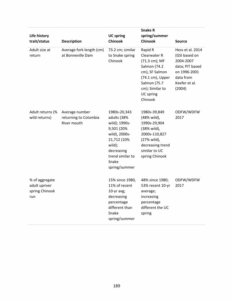
189
Life history
trait/status Description
UC spring
Chinook
Snake R
spring/summer
Chinook Source
Adult size at
return
Average fork length (cm)
at Bonneville Dam
73.2 cm; similar
to Snake spring
Chinook
Rapid R
Clearwater R
(71.3 cm); MF
Salmon (74.2
cm), SF Salmon
(74.1 cm), Upper
Salmon (75.7
cm); Similar to
UC spring
Chinook
Hess et al. 2014
(GSI based on
2004-2007
data; PIT based
on 1996-2001
data from
Keefer et al.
(2004)
Adult returns (%
wild returns)
Average number
returning to Columbia
River mouth
1980s-20,343
adults (38%
wild); 1990s-
9,501 (20%
wild), 2000s-
21,712 (10%
wild);
decreasing
trend similar to
Snake
spring/summer
1980s-39,849
(48% wild),
1990s-29,904
(38% wild),
2000s-110,827
(27% wild),
decreasing trend
similar to UC
spring Chinook
ODFW/WDFW
2017
% of aggregate
adult upriver
spring Chinook
run
15% since 1980,
11% of recent
10-yr avg;
decreasing
percentage
different than
Snake
spring/summer
48% since 1980;
53% recent 10-yr
average;
increasing
percentage
different the UC
spring
ODFW/WDFW
2017

190
Appendix C. Review of Appendix C in Murdoch et al. (2011)
Appendix C of Murdoch et al. (2011) presents methods for comparing abundance and
productivity (the performance measure) between reference and supplemental populations.8
There are many potential reference populations and there is concern that the set of potential
reference populations differ in their “closeness” to the supplemental population on the
performance measure during the period before supplementation is started.
A measure of the effect of supplementation is computed for each pair of reference vs.
supplemented stream. Individual estimates of effect size are obtained for each pair of
supplemental vs. reference stream.
This review examines each section in the Appendix C of Murdoch et al. (2011) and makes some
recommendations to improve the document.
C.1. Selecting Reference Populations
The authors are commended in their careful search for reference streams using a number of
criteria listed on page 199 of Appendix C of Murdoch et al. (2011). Some of the criteria are
biologically based (e.g., similar life history) while other criteria are statistical (e.g., accurate
abundance estimates or a long time series). The statistical criteria have little bearing on the
suitability of a reference stream; the impacts of these criteria are on the precision of the
estimates. For example, if there is substantial measurement error in estimates of abundance or
if the time series is short, estimates of the supplementation effect are still unbiased, but the
standard error of the supplementation effect may be so large that effects of supplementation
have low power to be detected (refer to Appendix E). With suitable methodology, there is some
benefit to including reference streams in the analysis that have substantial measurement error
or short time series. All else being equal, the biological criteria should be given more weight in
selecting the reference streams than the statistical criteria.
The appendix uses several measures of “closeness”:
1. Correlation in performance measure (e.g., abundance) during the period before
supplementation occurs
2. Graphical comparison of trends over time
3. Comparing the slopes of any trends over time
4. Comparing the minimal detectable difference
8 The material in Appendix C of Murdoch et al. (2011) was essentially duplicated in Appendix 6 of Hillman et al. (2017).

191
The graphical methods compare population (potential reference vs. supplementation stream)
on three measures (abundance, natural origin recruits, and adult productivity). The comparison
was done on both the actual scale and natural logarithm scale. A priori, a logarithmic scale
would be preferred. Abundance values vary from year-to-year based on year-specific effects
(see Appendix E). In many biological systems, these effects are multiplicative, i.e., in a good
year the number of spawners may increase from 100 to 150 in one stream and from 50 to 75 in
another stream. While the arithmetic difference is not equal (differences of 50 vs. 25), both
streams experience a 50% increase in abundance or a change of log(1.5)=0.4 on the logarithmic
scale resulting in more “parallelism” in their responses over time as noted by the authors on
page 202 of Murdoch et al. (2011).
Next, a correlational analysis was used to evaluate reference streams vs. the supplementation
stream. The authors are too pessimistic about the need for a high correlation between the
performance measure in reference and supplemental streams prior to the period of
supplementation. In the case of BACI designs, the purpose of the reference stream is to simply
show the change in the mean response over time between the before and after periods. This
difference is compared to the change in the MEAN response in the supplemental stream
between the before and after periods (see Appendix E). If this differential change in the MEAN
(the BACI effect) is not zero, then there is evidence that supplementation has an effect.
Consequently, the correlation in actual responses between the two streams could be zero and a
valid estimate of the BACI effect can still be obtained. There is no statistical reason why a
correlation of at least 0.6 is needed (page 209 of Murdoch et al. 2011). However, the PRECISION
(the standard error) of the BACI estimate is affected by the correlation in responses between
the streams during the before period, which is largely driven by any year-specific effects that
are common to both populations.
Consequently, it is NOT necessary to select reference populations that have a high correlation
with supplemental streams as long as the MEAN performance measure is estimated well in
both periods (before vs. after).
The standard BACI design assumes that the performance measure is in steady state prior to and
after the supplementation starts (see Appendix E). The authors (page 209 of Murdoch et al.
2011) computed the trend in all streams and examined if the trend could be distinguished from
the trend observed in the supplementation stream. The standard statistical technique to do this
is Analysis of Covariance (ANCOVA), but it is unclear from the text if the authors actually did
this. The authors did a trend analysis on both the original and logarithmic scale. Again, a priori,
the logarithmic scale should be the preferred scale. It turns out that a BACI analysis is still valid
in the presence of parallel trends if the effect of supplementation is a shift in the intercepts
without any changes in the slopes. If the effect of supplementation is a change in the slopes,

192
then a BACI analysis (or the equivalent paired difference approach used by the authors) will
need to be modified.
Too often studies are conducted without a proper investigation of the power of a particular
design. The power analysis conducted by the authors (page 212 of Murdoch et al. 2011) is
appropriate based on the empirical estimates of variation computed by pairing of the
supplemental stream with each of the reference streams. The power analysis of the ratio would
be more appropriate when computed on the log(scale), i.e., log(T/R) as this then corresponds to
the paired-difference approach on the log(performance measures). The resulting minimal
detectable difference can be re-expressed on the original scale by taking the anti-logarithms
which would be more easily understood. For example, if the minimal detectable difference of
log(T/R) is 0.60, this implies that a multiplicative change of exp(0.60)=1.8x can be detected.
Finally, the authors develop a procedure to score which reference stream is “best” based on 5
criteria (top of page 220 of Murdoch et al. 2011). The criteria can again be divided into
biological criteria (pre pNOS and post pNOS) and statistical criteria (correlation, relative
difference in slopes, and a coefficient of variation). Each criterion is considered to be
independent in developing a metric (Table 11 of Murdoch et al. 2011). Unfortunately, the three
statistical criteria are all highly correlated and some double counting is taking place. For
example, if the response measure is highly correlated between the two streams, then the
trends will be similar and the CV value also higher. The statistical criteria also influence the
precision of the BACI estimate and have no impact on the bias of the BACI estimate. The
statistical criteria should be given little weight in deciding on an appropriate reference stream.
C.2. Analysis Methods
C.2.1. Analysis of Trends
The authors compared the slopes within each supplemental-reference pair for each period
(before and after) using what appears to be Analysis of Covariance (ANCOVA), but this
technique was never explicitly mentioned. Unfortunately, the analysis did not directly examine
if supplementation had a positive effect – rather the authors hoped that a parallel trend in the
before period would be replaced by a non-parallel trend in the after supplementation period.
A direct examination of the relevant hypothesis is possible using a variant of ANCOVA
combining data from both periods and both streams using a similar approach as a BACI analysis.
A model of the form:
𝑌 = 𝑆𝑖𝑡𝑒 ∗ 𝑃𝑒𝑟𝑖𝑜𝑑 + 𝑌𝑒𝑎𝑟 ∗ 𝑆𝑖𝑡𝑒 ∗ 𝑃𝑒𝑟𝑖𝑜𝑑

193
could be fit. Here the term Site:Period corresponds to the 4 intercepts for the 4 different trends
(2 sites x 2 periods) and the term Year*Site*Period would directly test (and estimate) if the
CHANGE in slope for the supplemental stream between the before and after periods is the
same as the CHANGE in slope for the reference stream between the before and after periods.
The author’s and the above analysis allowed the intercept for the trend lines to vary between
periods leading to disconnected lines see in Figure 8 (and others in Murdoch et al. 2011) when
supplementation starts. It is also possible to modify the above analysis to allow for a broken
stick trend line where the trend lines for a site in the before and after periods must join at the
start of supplementation. This model should also be explored.
All of the analyses can be done on the original scale or the logarithmic scale, but as noted
earlier, the logarithmic scale is preferred.
C.2.2. Analysis of BACI Data
The authors used a paired-difference approach where the difference, ratio, or difference annual
change was computed for each year, followed by a t-test of the difference/ratio comparing the
mean difference/ratio/change before and after supplementation started. This is equivalent to a
BACI analysis using a mixed linear model (see Appendix E.1).
It is not necessary to test if variances are equal (see p.231 of Murdoch et al. 2011) in the before
vs. after periods as the Aspin-Welch version of the t-test performs well even if variances are
unequal. The tests for normality may also be superfluous because the sample size is reasonable
in both periods, so the central limit theorem implies that the results are robust to non-
normality.
It is puzzling that the authors were unable to perform a one-sided randomization test, as
randomization tests, per se, are not restricted to one-sided hypotheses?
We agree with the authors (p. 232 of Murdoch et al. 2011) that no adjustment is needed for
autocorrelation because of the small number of years measured.
Separate analyses were done on the three performance measures on both the original and log-
transformed values using differences/ ratios/ changes. As noted earlier, the analyses on the log-
scale will be preferred. Results from such analyses (e.g., Table 15 of Murdoch et al. 2011)
should be converted to the multiplicative change (e.g., an effect size of .701 on the log-scale
corresponds to an exp(.701)=2x change on the original scale.
C.2.3. Corrections for Density Dependence
Two different corrections for density dependence were employed.

194
In the first method, the recruits/spawner were adjusted by the carrying capacity. This method
will only have an impact when the number of spawners exceeds capacity.
In the second method, a fraction of carrying capacity was computed. Because all values of NOR
for a stream are divided by the same constant, the results from this analysis will be identical
when a log-transform is used to the analysis of log(NOR) seen earlier because
log(NOR/K)=log(NOR) – log(K) and log(K) is constant for all years. This was noted by the authors
in a footnote on page 251 pf Murdoch et al. (2011). Analyses using this correction therefore
provide no new information.
Both of these methods require an estimate of capacity. This was estimated using a Ricker,
Beverton-Holt, and a hockey-stick model. The authors use a non-linear regression method to fit
these models and compare models using information theoretic methods (AICc). All models had
virtually the same AICc values indicating that there was little to distinguish among them, but
the authors decided to use only the results from the hockey-stick model. A more natural
approach would be to use model averaging to average the estimated capacity from all three
models.
The analysis of the corrected-for-density dependence measures uses the same methodology as
other measures and similar comments apply.
C.2.4. Comparing Stock Recruitment Curves
The authors used a randomization approach to examine if there was evidence that the stock-
recruitment curves differed between supplemented and reference streams when each pair of
streams was examined.
The authors tested two hypotheses – first that the model parameters are indistinguishable
between streams and second that the fitted curve differed somewhere along the curve. The
randomization procedure used an ad hoc discrepancy measure.
It is no more difficult to actually fit models with both parameters in common, only one
parameter in common, or no parameters in common and use AICc to rank these models to
determine the degree of support for a common stock-recruitment curve. This approach would
be preferred to that taken by the authors.
The second hypothesis is redundant – if the underlying parameters cannot be distinguished
between the two populations, then the results curves cannot be distinguished. The second
hypothesis can be dropped.

195
C.2.5 Analyses without Reference Populations
The authors discuss several approaches to look at changes between the before and after period
without a reference stream.
First, a before vs. after comparison of the slopes in each period using a t-test. This is a variant of
ANCOVA (despite this method not being mentioned by the authors). As well, models where the
trend lines match at the start of supplementation should also be considered.
Second is a before vs. after comparison of the means using a two-sample t-test. This is
standard.
Third is a comparison of stock-recruitment curves. The authors used an ad hoc randomization
approach rather than an AICc directed approach as noted earlier.
Fourth is a correlational approach looking at the relationship between pHOS and productivity
using a standard correlational analysis. This is standard but likely has low power to detect
effects.
Lastly is a comparison to standards. No analysis is presented for this approach.
The key problem with before vs. after studies is the effects of periods are completely
confounded with temporal changes in any other variables between the two periods.
Consequently, these methods should seldom be used.
C.2.6. Review of Conclusions in Appendix C
The authors did painstaking work to identify appropriate reference streams based on biological
and statistical criteria. More weight should be given to the biological criteria and less to the
statistical criteria. The statistical criteria affect the precision of the estimates, but not the bias
of the estimate of the BACI effect.
The authors recommended analyses based on paired differences on the original scale (T-R) or
ratios (T/R). We disagree with the last recommendation. Many effects in biological populations
are multiplicative rather than additive, and log(T/R) or log(T)-log(R) would be more appropriate,
i.e., analyze the log(response measure).
The first corrections for density dependence seem sensible, but the second has no impact if the
analysis is done on the logarithmic scale because the new response measure is a simple scaling
of the original data. The second method is akin to analyzing the data in ‘000s of fish vs. an
analysis using the actual number of fish. Both methods rely on estimates of carrying capacity.
The AICc criterion indicated that several models seem to fit the data equally well – rather than
selecting the carrying capacity from a single model, a model-averaged values should be used.

196
The comparison of stock-recruitment curves among pairs of populations was performed using a
randomization test using an ad-hoc measure of discrepancy. AICc methods should be used to fit
and rank 4 models that differ in the number of common parameters between the two stocks.
C.3. Summary and Recommendations
For the most part, the analyses are suitable and the conclusions drawn appropriate. However,
the report can be improved in the following ways:
1. Give more weight to biological criteria and less weight to statistical criteria to selecting
reference streams. Reference streams are still valuable if they match on the biological
criteria but not the statistical criteria.
2. Many biological systems have effects that operate multiplicatively. Consequently,
analysis of the log(performance) measure are often most suitable. In the paired
difference analysis, this is equivalent to an analysis on the log(T/R).
3. Some of the statistical methods used to estimate carrying capacity and compare stock-
recruitment curves need revision
4. Some of the statistical methods to compare trend lines between before and after
periods need revision.
5. Rather than presenting estimates of the supplementation effects in tables, a graphical
presentation should be created showing the estimate and measure of precision to make
the results more readable.
6. There are separate analyzes in this paper for each pair of supplemented stream and
reference stream, but the results are never aggregated together. A more sophisticated
analysis that used the combined set of the supplemental stream and all reference
streams, would lead to estimates with improved precision and have increased power to
detect effects (see Appendix E). In most cases, these models can be fit using standard
software (e.g., R), but there are some advantages to using Bayesian methods. For
example, a Bayesian analysis could incorporate prior belief on the benefit of
supplementation; integrate several performance measures; and more easily deal with
unequal variances over time in the different streams. Furthermore, the output from a
Bayesian analysis would provide a degree of belief rather than a simple yes/no from
standard hypothesis testing.

197
Appendix D. Additional Editorial Comments on Murdoch et al. (2011)
These additional comments do not relate directly to the charge to the ISAB in Section V (RME)
but are provided for completeness.
D.1. Editorial Comments on Appendix A of Murdoch et al. (2011)
The authors first develop a method to estimate the number of NOR in a multistep process.
(1) Total number of spawners returning is estimated in a multistep process from redd counts.
Redd counts from a single sample are adjusted to account for detection efficiency from a single
sample. Each redd accounts for a single female. An expansion factor is used to adjust for the
male:female adults ratio and then for the jacks:total population ratio (see comment below on
page 166).
(2) The total escapement is then multiplied by the sex ratio seen in broodstock and carcass
surveys to estimate the number of wild fish. Here some problems could occur because the total
escapement includes jacks, but because jacks are smaller, they may be underrepresented in
carcass or excluded in broodstock surveys. The first problem is noted on the bottom of page
169. There are also some editorial problems as noted below where the numbers in the text for
examples don’t match the Tables.
(3) The estimated wild fish from (2) are then multiplied by the age distribution to get the
number of wild fish by brood year x age. See comments below on p. 169 of Murdoch et al.
(2011)
(4) The brood year x age values are summed over all ages for brood year to get the number of
wild fish returning for a particular brood year.
(5) The values in (4) are adjusted for harvest using either a hatchery indicator stock or a harvest
report from the Joint Staff reports. It is also adjusted for handling mortality (recreational,
commercial, or non-selective harvests) as well.
The NRR is computed by natural returns for a brood year / total escapement that produced
these returns.
The methods used seem reasonable. The key problems are making sure that the various
expansion factors are sensible and correct as used. There are many places where biases can be
introduced such as non-random sampling (harvest, carcass searches). There is no easy way to
estimate the potential size of biases that may occur, but this may be moot given the extreme
drop in the stocks seen in Figure 1 of Appendix A of Murdoch et al. (2011).

198
There are quite a few places where the numbers in the text don’t agree with the numbers in
the tables as shown below so some editorial changes are needed.
p.166. The expansion factor for jacks isn’t quite correct. The correct expansion factor is 1/(1-p)
where p is the proportion of jacks. For example, if jacks are 50% of the run, then the number of
adults must be doubled to account for jacks + adults. If jacks are 14% of the run, then correct
expansion factor is 1/(1-.14)=1.16 not 1.14.
p.166. It is not necessary to make the assumption that male mate with only one female.
p.167. Something doesn’t add up. They claim the proportion of wild fish is 0.24, yet Table 2 of
Appendix A of Murdoch et al. (2011) has a value of 0.21. They also claim a wild return of 589,
but 0.24 x 1725 = 414. The difference isn’t the wild fish retained in the brood stock – Table 2 of
Appendix A of Murdoch et al. (2011) has this as 115 fish.
p.169. Values used in brood year example don’t match Table 3 of Appendix A of Murdoch et al.
(2011). For example the text has a proportion of 0.020 for age-3 fish in 2004, but Table 3 of
Appendix A of Murdoch et al. (2011) has 0.060.
D.2. Editorial Comments on Appendix B of Murdoch et al. (2011)
Stray rates for steelhead and sockeye are based on location of last detection of fish that have
PIT-tags. It wasn’t clear if all streams in the system have PIT-tag arrays to detect fish – if not,
then stray rates may be underestimated. For example, if 10% of fish go to a stream without a
PIT-tag array, then these fish are “invisible” and are not counted as strays. See for example,
p.187 of Murdoch et al. (2011) where the authors comment on new PIT-tag array sites being
established over time. The methodology seems ok.
Stray rates for Chinook are based on CWT expansions for tagging proportions and catch
searched. Methodology seems OK.
However, statements such as found on page 192 of Murdoch et al. (2011) that the stray rate
is more than 5% based on these raw estimates are unfounded because no measures of
uncertainty were presented. For example, there is no standard error presented for any
estimate of stray rates so it is unclear if the 17% stray rate estimate has an uncertainty of ±1
percentage point or ±15 percentage points.
The authors then looked at what fraction of given escapement are strays. This was not done for
PIT-tagged studies as the fraction tagged is unknown. This was done using CWT for Chinook.
Again, no estimates of uncertainty are produced so it is difficult to evaluate if the average
proportion of strays meets targeted values.

199
There is a comment on the bottom of page 194 of Murdoch et al. (2011) about changes in
survey effort being confounded with estimates of stray rates. The Tables would be
strengthened if some estimates of survey effort were added to see when the survey effort
expanded dramatically.
D.3. Editorial Comments on Appendix C of Murdoch et al. (2011)
p.3. As noted in the review of Appendix C of Murdoch et al. (2011), it is not necessary that
reference streams “track” supplemental streams with a high correlation. The choice of
reference streams should be based more on biological criteria than statistical criteria.
p.3. As noted in the review of Appendix C of Murdoch et al. (2011), we suggest they use the
log(T/R) rather than just T/R. There are two reasons. First, many effects operate
multiplicatively, and so analyses on the log() scale are preferred. Secondly, the analysis of T/R
could give quite different results than the analysis of R/T (e.g., 2/1 is quite different than 1/2
relative to no effect of a ratio of 1). However log(2)= -log(1/2) so the analysis of log(T/R) and
log(R/T) is symmetric and only the sign changes.
So all of the hypotheses listed on pages 3 of Appendix C of Murdoch et al. (2011) onwards
about mean ratio scores would be better done using mean log(ratio) scores etc.
p.4. Assumption of normality is not important given the relatively large number of years of data
available.
p. 5. It is not clear how they intend to compare the distribution of redd locations. If they want
to measure the mean river location that is not really a test of distribution of the redd locations.
It is not clear here what statistical method will be used for hypothesis 2.3. Figure 7 of Appendix
C of Murdoch et al. (2011) indicates that a simple test of the MEAN river location will be used
so the hypothesis needs to be rewritten in terms of the mean river mile of redds.
p.6. Hypothesis 3.2 appears to be a way to test for no trend. Similarly, Hypothesis 3.3 is a way
to state no trend.
p.6. Hypothesis 3.4 should likely test if the MEAN ages of maturity are equal. Looking ahead at
page 28, this is what is done, i.e., testing if the mean age changed. There is no reason why a
Kruskall-Wallis test (see page 28) needs to be used for this comparison as a regular two-way
ANOVA as used for mean Julian date of return or spawning or redd locations will work just fine.
p.10. A hypothesis-testing framework seem an odd way to determine if management goals are
being met. Is the management goal stated in terms of long-term averages or is there a specific
target that must be met? It seems to us that this is a yes/no answer without the need for a
formal hypothesis testing framework.

200
p.19. All four reference streams should be used together in a single analysis as outlined in our
review of Appendix C rather than this ad hoc weighting scheme. This would give an overall
value for Table 6 rather than each individual supplementation vs individual reference stream
result. You also have improved power to detect effects – for example, none of the individual
comparisons for productivity showed evidence of an effect, but a combined analysis may show
evidence of an effect.
p.28. No reason why a Kruskall-Wallis test should be used. Use a two-way ANOVA in a similar
fashion to test if the mean Julian date, or mean redd location differed between groups.
p.29. Graphs are labeled as “mean total age.” Likely should be just “mean age.”
p.31. See earlier comments about comparing management objectives through hypothesis
testing. The proportion of time management objectives are not met is important. Each of the
values in Table 8 (the HRR and NRR) needs a measure of uncertainty to compare against
management objectives of 4.
Similar comments as above about other population analyses. Some specific comments are:
p. 52. Figure 27. What happened to the redd distribution in 2010?
p. 57. Figure 33. Need SE on the bars.
p. 58. The authors concluded that a small sample size can cause an effect to be detected. This is
unlikely to be true.

201
Appendix E. Review of BACI Analysis
This appendix reviews the details of a BACI analysis to understand what assumptions are being
made and the impact of violations of these assumptions.
E.1. One Supplemented and One Reference Stream
Consider first a BACI design with one stream receiving supplementation and the other stream
serving as reference with both streams measured for 10 years before and 10 years after
supplementation is started (in year 11). For simplicity, assume that the mean number of
spawners on the spawning grounds does not change between the before and after periods for
the control stream, but increases for the supplemental stream.9 All analysis takes place on the
logarithmic scale so that the effect of augmentation is a multiplicative effect rather than an
additive effect.
Suppose that the TRUE mean log(number of spawners) in both streams in both periods (before
vs. after) is shown in Table E.1.
Table E.1. Mean abundance in two streams, before and after supplementation is started
Stream Mean during BEFORE
period Log(mean)
Mean during AFTER period
log(mean)
Reference 200
5.30
200
5.30
Supplemented 300
5.70
400
5.99
The BACI analysis looks for a differential change, i.e., the difference in change in the log(mean)
for the reference stream between the before and after periods vs. the change in the log(mean)
for the supplemented stream, i.e.
(log(𝑚𝑒𝑎𝑛)𝑠𝑢𝑝,𝑎𝑓𝑡𝑒𝑟 − log(𝑚𝑒𝑎𝑛)𝑠𝑢𝑝,𝑏𝑒𝑓𝑜𝑟𝑒) − (log(𝑚𝑒𝑎𝑛)𝑟𝑒𝑓,𝑎𝑓𝑡𝑒𝑟 − log(𝑚𝑒𝑎𝑛)𝑟𝑒𝑓,𝑏𝑒𝑓𝑜𝑟𝑒)
or in this case
(5.99 − 5.70) − (5.30 − 5.30) = 0.28
9 The analysis and conclusions are identical if the control stream has a change in the mean between the before and after periods.

202
representing an exp(0.28) = 1.33x times larger (multiplicative) change in the mean abundance
in the supplemented stream (a 1.33x increase) compared to the reference stream (a 1.0x
increase). This is known as the BACI effect.
Actual data will not fall exactly on the means and there are several sources of variation (Figure
E.1).
year-specific effects (e.g., weather) which affects returns to both streams equally. In the simple BACI experiment, these effects have a variance of 𝜎𝑦𝑒𝑎𝑟
2 which affects streams
simultaneously. For example, if ocean conditions are such that abundances in a year increase, the same increase should be seen in all streams.
year-site interaction effects that represent the non-parallelism of response between the
supplemented and reference sites with a variance of 𝜎𝑠𝑖𝑡𝑒−𝑦𝑒𝑎𝑟2 which is assumed the
same for all years and all sites.
measurement error where the actual abundance is measured with error. This is completely confounded with the year-site interaction effects and so will be “ignored.”
Figure E.2 presents three scenarios of simulated data where the year-specific variance is the
same in all scenarios, but the year-site interaction variance differs. The figure also presents the
correlation between the measurements along with estimates of the BACI effect (see below)

203
Figure E.1. Conceptual sources of variation in a BACI experiment with 1 supplemental stream (S) and one reference stream (R). Year-to-year variation represents year-specific effects that are equal in both streams. Site-year interaction represents non-parallelism in the response over time. This is confounded with measurement error and cannot be separated. The difference in the means during the before period is due to intrinsic site-to-site differences. The difference in the means during the after periods is due to the intrinsic site differences plus the effect of supplementation.

204
Figure E.2. Simulated results under three scenarios. In all scenarios, the variance of the year-specific
effect is held fixed (𝜎𝑦𝑒𝑎𝑟2 = 1) while the year-site interaction effects vary as shown on the plot. The
study was conducted using the means shown in Table E.1 with measurements taken 10 years before the supplementation program began and 10 years after the supplementation started.

205
There are two equivalent ways to estimate the BACI effect. First (as was done in Appendix C of
Murdoch et al. 2011), the yearly values for the reference and supplemented streams are paired
and the difference between the two (e.g., supplemented – reference measurement) is taken.
This reduces the data to a single “difference” for each year, and two-sample t-test that the
mean difference is the same in the before vs. the after period can be computed.
Second, a formal BACI model can be file (refer to Section 12.9 in
people.stat.sfu.ca/~cschwarz/Stat-650/Notes/PDFbigbook-R/R-part013.pdf ). The model is
(using a standard modelling syntax)
𝑌 = 𝑆𝑖𝑡𝑒 + 𝑃𝑒𝑟𝑖𝑜𝑑 + 𝑆𝑖𝑡𝑒: 𝑃𝑒𝑟𝑖𝑜𝑑 + 𝑌𝑒𝑎𝑟(𝑅)
where Site refers to the site effects (reference vs. control), Period refers to the effects of before
vs. after periods, and Site:Period represents the site-period interaction where the change
between the before and after period is the difference for the reference and supplemental
streams and represents the BACI effect; Year(R) represents the random year-specific effects
which are assumed to affect both sites equally. This model is a Mixed Linear Model and can be
fit using standard software (e.g., lmer() in R). A contrast of the Site:Period terms yields the BACI
effect.
The estimated BACI effects are shown in bottom right of Figure E.2. The true value of the BACI
effect (see above) is 0.28. In all scenarios, the estimated BACI effects are unbiased estimates of
the true BACI effect (0.28), but the standard error of the estimates varies considerably.
In addition, the (theoretical) correlation between the readings in the two streams during the
before period is shown in the upper right part of each plot for each scenario. It can be shown
that the correlation is found a 𝜎𝑦𝑒𝑎𝑟
2
𝜎𝑦𝑒𝑎𝑟2 +𝜎𝑠𝑖𝑡𝑒−𝑦𝑒𝑎𝑟
2 . Intuitively, the BACI effect is more precise when
the correlation is larger. However, the degree of correlation has NO IMPACT on the bias of the
estimates. Indeed, a valid BACI estimate can still be found even if the correlation between the
readings in the two streams is 0. The correlation between the readings in the two streams
during the before period will affect the precision of the estimates, but the BACI estimates are
still unbiased. Secondly, the precision of the BACI estimates “incorporates” the correlation
between the measurements in the two streams prior to supplementation. The standard error
provides a natural and defensible way to “rank” the reference streams.
E.2. One Supplemented and Multiple Reference Streams
The design can be extended by including several reference streams and simulated data in the
case with 1 supplemental stream and 3 reference streams is shown in Figure E.3. The BACI
206
effect represents the differential change between the mean for the supplemental site vs. the
differential change in the mean over ALL reference sites.
This BACI estimate can again be formed in two (equivalent) ways. First, three separate paired
analyses can be done as before using the supplemented stream vs. each of the reference
streams. This gives three estimates of the BACI effect, and they must now be combined.
Because we are assuming that the year-specific effect and year-site interaction effect variances
are the same for all stream, the overall BACI effect is found as a simple average of the three
individual BACI estimates (i.e., a weighted average with equal weights). However, the estimates
are NOT independent (the same supplemental steam is used in all three pairs) so the standard
error of this weighted average is not easily found.10
Secondly, a more complex mixed-linear model can be fit:
𝑌 = 𝐶𝑙𝑎𝑠𝑠 + 𝑃𝑒𝑟𝑖𝑜𝑑 + 𝐶𝑙𝑎𝑠𝑠: 𝑃𝑒𝑟𝑖𝑜𝑑 + 𝑆𝑖𝑡𝑒(𝑅) + 𝑌𝑒𝑎𝑟(𝑅)
where Site(R) refers to the random site effects (the single supplemental stream and the 3
reference streams); Class refers to the two classifications of the sites (supplemental vs.
reference); Period refers to the effects of before vs. after periods, and Class:Period represents
the class-period interaction where the change between the before and after period is the
different for the reference and supplemental streams categories and represents the BACI
effect; Year(R) represents the random effect of year. As before this model can be fit using
standard software (e.g., lmer() in R) and the BACI estimates found directly without having to
average the estimates from the three pairs.
Referring to Figure E.3, we once again can show that all estimates are unbiased; the precision of
the BACI estimates is improved relative to Figure E.2 (more than 1 reference stream
incorporated); the standard errors of the overall BACI estimate is found automatically without
having to average the results from the paired analysis. Once again, the correlation between the
readings among the streams during the before period will affect the precision of the
estimates, but the BACI estimates are still unbiased. Secondly, the precision of the BACI
estimates “incorporates” the correlation between the measurements among the streams
prior to supplementation. This more complex model will automatically “average” the
individual supplementation estimates from several reference streams.
10 The theoretical covariance between the three estimates depends only on the year-specific effects variance. In theory, this covariance could be used to find the standard error of the weighted average.

207
Figure E.3. Simulated results under three scenarios with 1 supplemented stream and 3 reference
streams. In all scenarios, the variance of the year-specific effect is held fixed (𝜎𝑦𝑒𝑎𝑟2 = 1) while the year-
site interaction effects vary as shown on the plot. The study was conducted using the means shown in Table E.1 with measurements taken 10 years before the supplementation program began, and 10 years after the supplementation started.

208
Both of the above analyses assumed that the year-specific effects had the same variance for all
streams, so that if the year-specific effect caused an increase in the log(abundance) in one
stream, it would cause the same increase in log(abundance) in the other streams. For example,
if the year-specific effect caused a doubling of abundance, then the increase in log(abundance)
would be log(2)=0.70 in both streams. A consequence of this assumption is that the variability
across time in all streams is equal. This assumption may be violated where the variability in one
stream is much larger/small than the variability in another stream. For example, year-specific
effect could result in an increase/decrease in log(abundance) in one stream by a factor of 0.7
(doubling or halving), but in the same year, could cause change in log(abundance) by a factor of
0.35 (1.4x change). There would still be a high correlation on the year specific effects.
Figure E.4 shows simulated data illustrating these ideas. In these scenarios, the reference
stream has a smaller variation over time than the supplemental stream. The year effects
between the two streams are correlated as shown on the plot. For example, in the lower panel,
there is a high correspondence in the two streams so that when the abundance in one stream
increases, the abundance in the other stream also increases, but not by the same quantity.
Similarly, decreases in abundance are matched. However, the BACI design “forces” the year
effect to be equal and so any non-parallelism seen here is assumed to be site-year variation and
so the “empirical” correlation smaller than the actual correlation.

209
Figure E.4. Simulated results under three scenarios with 1 supplemented stream and 1 reference
stream. The variability in the two streams differs (𝜎𝑠𝑢𝑝,𝑦𝑒𝑎𝑟2 = 1; 𝜎𝑟𝑒𝑓,𝑦𝑒𝑎𝑟
2 = .25) with different
correlations between the year specific effects. The study was conducted using the means shown in Table E.1 with measurements taken 10 years before the supplementation program began, and 10 years after the supplementation started. The panel label shows the correlation when the data was generated; the upper right value shows the correlation when the variability is divided into a common year effect and site-year interactions.
There are again two equivalent ways to analyze this data. In the paired analysis, the effect of
the unequal variances is “hidden” because the variance of the difference in a particular year is
𝜎𝑠𝑢𝑝,𝑦𝑒𝑎𝑟2 + 𝜎𝑟𝑒𝑓,𝑦𝑒𝑎𝑟
2 + 2𝜌𝜎𝑠𝑢𝑝,𝑦𝑒𝑎𝑟𝜎𝑠𝑢𝑝,𝑦𝑒𝑎𝑟 and so it doesn’t matter if the variances are equal
or different – the difference automatically has the appropriate variance.

210
If a BACI model is fit, the non-parallelism is assumed to be the effect of a common year-effect
and a site-year interaction. While the BACI analysis “forces” a common year effect, it also adds
a “year-site” effect to account for the non-parallelism and so again the final results are identical
to the paired analysis. This non-parallelism is again represented by the correlation in the
log(abundance) during the before period. Even with unequal variances, it can be shown that
the BACI estimates are unbiased and that the standard error of the estimate is related to the
correlation of the log(abundance). Once again, the standard error of the estimate is the best
measure for weighting the results from several reference streams because it incorporates all
sources of uncertainty.

211
Appendix F. Review of Hillman et al. 2017
F.1. Introduction
Hillman et al. (2017) present a five-year update to the Monitoring and Evaluation Plan being
used to evaluate the PUD hatchery programs in the Upper Columbia. Many of the methods in
their revised M&E Plan are similar to those presented in Murdoch et al. (2011). Here we
concentrate on issues that were not raised in our review of Appendix C that was part of
Murdoch et al. (2011). This review provides general comments about the Hillman et al.
document, followed by a chapter-by-chapter detailed review.
F.1.1. General Comment about Null Hypothesis Significance Testing
Hillman et al. (2017) make extensive use of null hypothesis statistical test (NHST, Appendix G) to
evaluate the impact of the supplementation program in the Upper Columbia. This is used in two
ways.
First is assessing if the impact of supplementation results in a change to a parameter that
measures the population. For example, consider the productivity indicator of abundance of
natural spawners (first row of Table 1 in Hillman et al. 2017). The supplementation program
should result in an increase in the mean number of natural spawners (the target change). The
null hypothesis is no change in the mean number of spawners from pre- to post-
supplementation. The test statistic is related to the observed difference in the sample mean
number spawners from the pre- and post-supplementation program. A large observed
difference (post-pre), accompanied by a small p-value, is evidence that the mean number of
spawners has increased with supplementation. A power analysis is used to ensure that enough
data (e.g., years of data pre- and post-supplementation) are collected to detect a certain
desirable change (e.g., an increase by at least 100 spawners).
Second, the program may wish to detect an adverse consequence from supplementation. For
example, consider the monitoring indicator of run timing (third row of Table 1 in Hillman et al.
2017). The supplementation program should result in no difference in migration timing
between hatchery and natural fish. The null hypothesis is again no difference in some
attribution of run timing (such as the mean arrival at the spawning grounds) between hatchery
and natural fish. The test statistic is related to the observed difference in the mean run timing.
A large difference in the mean run timing, accompanied by a small p-value, is evidence of an
adverse consequence of the supplementation program. Now a power analysis is used to ensure
that enough data are collected to detect an undesirable change (e.g., a change in run timing by
10 days).

212
In both cases, rather than just relying on a “reject” or “not reject” the null hypothesis
dichotomy, it is also useful to present estimates of the effect size along with measures of
uncertainty (e.g., standard errors or confidence intervals). When an effect is detected, the
estimated effect size will indicate if this is a large, biologically important effect or a small
(biologically non-important) effect that just happened to be detected because of a large sample
size. The actual p-value is NOT informative, i.e., the p-value could be 0.01 in both cases.
Similarly, if an effect is not detected, the estimated effect size will indicate if this is because it is
a small effect (with small uncertainty) or a potential large effect but with such a large
uncertainty, it was not detected. Again, the actual p-value is not informative, i.e., the p-value
could be 0.80 in both cases.
Consequently, when reporting the results from hypothesis testing, both the p-value and
estimates of effect size and measures of uncertainty must be reported. This last point needs to
be emphasized more in Hillman et al. (2017).
Null hypothesis testing is not really designed to assess “no impact” hypotheses. Given a large
enough sample size, it is almost certain that some effect will be detected, but it may not be
biologically relevant. To directly assess a “no impact” hypothesis, a modification to the NHST
framework may be useful, namely equivalence testing. The null hypothesis is defined as an
effect large enough to be deemed interesting, specified by an equivalence bound. The
alternative hypothesis is any effect that is less extreme than said equivalence bound. The
observed data is statistically compared against the equivalence bounds. In the two one-sided t-
tests (TOST) approach, two one-sided tests are performed with the null hypothesis being that
the effect size is less than/greater than the lower/upper bounds respectively. If both tests are
“rejected,” then there is evidence that the actual effect size is within the zone of indifference.
Equivalence testing reduces the misinterpretation of p-values larger than the alpha level as
support for the absence of a true effect. Furthermore, equivalence tests can identify effects
that are statistically significant but biologically unimportant. This method should be considered
as an alternative to regular NHST when the target direction in an indicator is no change.
The greatest disadvantage of the NHST framework is that it does NOT provide a direct answer
to the actual question – how certain is it that supplementation did or didn’t have an effect? The
p-value does NOT serve this purpose – the p-value measures the consistency of the data with
no effect, which is easily misinterpreted. Here a Bayesian approach may be useful. The
posterior belief about the parameter provides a direct interpretation of the question of
interest. For example, consider again the productivity indicator of abundance of natural
spawners (first row of Table 1 in Hillman et al., 2017). Under the NHST framework, a p-value of
0.02 indicates that the observed data is not consistent with no effect – hardly an interpretation
that can be understood with ease. Under a Bayesian framework, a posterior belief of 0.98 that

213
the mean abundance has increased under supplementation is easily interpreted. For most of
the analyses used in this document, a Bayesian analysis is easily implemented.
F.2. Review of Section 1 of Hillman et al. (2017)
Section 1 of Hillman et al. (2017) presents an overview of the monitoring and evaluation plan.
As noted by the authors, any management action needs to be evaluated for its effectiveness
and a suite of outcomes from management is presented in their Figure 1 and their Table 1
(called indicators in their document). These outcome variables have been divided into two
classes – monitoring indicators and productivity indicators (using their terminology) with the
main distinction being that productivity indicators are the primary metrics to assess if
conservation and safety-net goals have been met, with the monitoring indicators being used if
the productivity indicators are not available or results are equivocal.
Their Table 1 presents a summary of the direction in which each of the monitoring and
productivity indicators should be moving if the management actions are successful. These
directions drive the statistical hypotheses created to evaluate the program. For example, the
target direction for the abundance of natural spawners is an increase. The statistical hypothesis
associated with this indicator will have a null hypothesis of NO change and an alternate
hypothesis of an increase after supplementation. Thus the “rejection” of the hypothesis will
provide evidence of a program success. On the other hand, the target direction for adult
productivity (NRR) is no decrease. The statistical hypothesis associated with this indicator will
have a null hypothesis of no change and an alternate hypothesis of a decrease in NRR after
supplementation. Now failure to reject the hypothesis will be an indication of program success!
As noted previously, the null hypothesis significance testing framework is less useful when
monitoring for no change.
All indicator variables should relate directly to the populations such as abundance, juveniles per
redd, pHOS etc. which are easy to interpret. But, their Table 1 also includes some indicators
that cannot be directly measured in the populations such as Residuals vs. pHOS or Effective
population size or Genetic Distance, which are statistical measurements and are much harder
to interpret. Presumably, the latter should be given less weight when evaluating management
actions, but this is never indicated in the document. These indicators need to be replaced by
parameters that are directly measurable (see later sections below).
Their Table 1 also includes some indicators for which it is not obvious what is being compared.
For example, indicators such as migration timing could be compared in terms of the entire
distribution, of the mean arrival time, or of selected percentiles. These are explained in more
detail later in the document, but their Table 1 could be updated with footnotes to indicate
upon which dimension these indicators will be compared.

214
There is no guidance provided in Section 1 on how to weight the monitoring indicators
“In the event that the statistical power of tests that involve productivity indicators is
insufficient to inform sound management decisions, some of the monitoring indicators
may be used to guide management.”
Are changes in migration timing and distribution, for instance, more important than changes in
redd distribution? This section could be improved by ranking the indicator variables in terms of
importance to assessing the program.
To evaluate the impact of management actions, there is a need to account for temporal change
to separate out the effect of management actions and temporal changes that would have
occurred in the absence of management actions. The key design for such comparison is a
Before–After-Impact-Control (BACI) design (and variants). A reference population is required
that does not undergo management actions in order to measure temporal effect. There is a
brief discussion in their Section 1 on how to assess impact in the absence of suitable reference
populations. The authors should review Wiens and Parker (1995) for advice on dealing with
such situations and update this section of the document.
F.3. Review of Section 2 (Adult Productivity) of Hillman et al. (2017)
This section provides a detailed protocol on how to assess the Adult Productivity indicators. For
each indicator, a detailed monitoring question is provided along with formal statistical
hypotheses to be examined from the monitoring study. For each indicator, what variables are
measured or derived is given along with the frequency with which the indicator is measured.
F.3.1. Review of Section 2.1 (Natural Replacement Rate (NRR))
The NRR is defined as
The number of natural origin recruits (NOR) is computed on a brood year basis. From their
Table 1, the NRR should not decrease if management actions are successful.
A set of six statistical hypotheses are presented – the authors indicate that the choice among
the hypotheses will depend on the quality and quantity of the data available.
Because the target direction for this indicator is no increase, the statistical null hypothesis of no
change was translated to a null hypothesis of program success, and a “rejection” of the
hypothesis would provide evidence of a program failure.

215
Presumably, the intent is actually the reverse, i.e., until evidence provides elsewise, the status
quo is that supplementation has no impact. All of the hypotheses should then be reversed in
this section. If the intent is actually to assume equivalency until proven otherwise, then
equivalence testing should be used.
This reversal of the null hypothesis implies that standard power computations are not
informative because they provide information on the ability to detect failure and not success.
As noted in the previous review of Appendix C, hypotheses about the ratio of the NRR between
supplemented and reference streams should be expressed in terms of the log(ratio).
(Hypotheses 4 and 5) and difference in the slopes of NRR should be analyzed on the log() or
logit() scale for the same reason (Hypothesis 2).
Hypothesis 6 is not a proper statistical hypothesis because it depends on data (the residual
from a fit) and not the underlying population metrics (the mean NRR or slope of the NRR line).
This needs to be recast by hypothesizing that the addition of pHOS has no impact on the stock
recruitment curve, i.e., similar to a multiple regression hypothesis that a certain variable has no
marginal impact on the fit. A correlation analysis is not appropriate here.
The list of possible statistical methods should include a BACI analysis and a paired t-test method
when a reference stream is available (see companion review of Appendix C). Both methods are
equivalent when there is a single reference stream, but a BACI analysis can be extended when
there are multiple reference streams.
The authors suggest that
“Correlation analysis will examine associations between hatchery adult composition and
NRRs.”
There does not appear to be a definition of hatchery adult composition in this document. Does
this mean pNOB (the proportion of the broodstock consisting of NORs)? If the hatchery adult
composition is a proportion of some sort, then ordinary regression analysis should be used
rather than correlational analysis as it will be more informative.
The suggestion that productivity should be correlated with other factors such as ocean
productivity in a particular five-year period will have essentially no power to detect effects
because of the very small sample size (5 years).
F.3.2. Review of Section 2.2 (Natural Origin Recruits (NOR))
The NOR is defined as number of natural origin returns (NOR) computed on a brood year basis.
From their Table 1, the NOR should increase if management actions are successful.

216
A set of six statistical hypotheses are presented – the authors indicate that the choice among
the hypotheses will depend on the quality and quantity of the data available.
Because the target direction for this indicator is an increase, the statistical null hypothesis of no
change implies a null hypothesis of program failure, and a “rejection” of the hypothesis would
provide evidence of a program success. This is a situation where the null hypothesis significance
testing framework is most often used. The resulting p-value does not have an easy
interpretation, and a Bayesian approach may be more useful.
As noted in the companion review of Appendix C, hypotheses about the ratio of the NOR
between supplemented and reference streams should be expressed in terms of the log(ratio).
(Hypotheses 4 and 5) and difference in the slopes of NRR should be analyzed on the log()scale
for the same reason (Hypothesis 2).
Hypothesis 6 again suffers from the problem that the status quo is that supplementation is
working and a “rejection” of the hypothesis is an indicator of failure (see previous section). If
this is the intent, then equivalence testing is preferred over a simple hypothesis test.
The list of possible statistical methods should include a BACI analysis and a paired t-test method
as noted previously.
Hatchery adult composition is not defined and a regression analysis may be more informative
(see previous comments).
The suggestion that productivity should be correlated with other factors such as ocean
productivity in a particular five-year period will have essentially no power to detect effects
because of the very small sample size (5 years).
F.4. Review of Section 3 (Juvenile Productivity) of Hillman et al. (2017)
This section is structured similarly to Section 2 of Hillman et al. (2017) (reviewed earlier).
The key productivity indicator is the number of juveniles/redd. There are two monitoring
questions. First, is there a general change in juveniles/redd between the years with and without
supplementation. Second is there a specific relationship between juveniles/redd and the
proportion of hatchery spawners (pHOS).
Their Table 1 is not consistent with this section. The first productivity indicator for juvenile
productivity in Table 1 is Residuals vs. pHOS; the second indicator is juveniles per redd vs.
pHOS. Neither of these are indicators, but rather statistical tests, and both should be replaced
simply by juveniles/redd.

217
A set of six statistical hypotheses are presented for the general change and two for the specific
relationship – the authors indicate that the choice among the hypotheses in each group will
depend on the quality and quantity of the data available.
F.5.1. General Investigation of Impact of Supplementation on Juvenile Productivity
All of the hypotheses are framed in terms of detecting negative effects of supplementation.
Equivalence testing may be a more suitable methodology rather than standard null hypothesis
testing. The hypotheses in this section need to be updated in conjunction with changes to their
Table 1.
As noted in the companion review of Appendix C, hypotheses about the ratio of the
juveniles/redd between supplemented and reference streams should be expressed in terms of
the log(ratio). (Hypotheses 4 and 5) and the difference in the slopes of juveniles/redd should be
analyzed on the log()scale for the same reason (Hypothesis 2).
Hypothesis 6 is not a proper statistical hypothesis because it depends on data (the residual
from a fit) and not the underlying population metrics (the mean juveniles/redd or slope of the
juveniles/redd line). This needs to be recast by hypothesizing that the addition of pHOS has no
impact on the stock recruitment curve, i.e., similar to a multiple regression hypothesis that a
certain variable has no marginal impact on the fit. A correlation analysis is not appropriate here.
Hypothesis 6 also suffers from the problem that the status quo is that supplementation is
working and a “rejection” of the hypothesis is an indicator of failure (see previous section). If
this is the intent, then equivalence testing is preferred over a simple hypothesis test.
F.5.2. Specific Investigation of the Relationship between pHOS and Juvenile Productivity
The target direction for this indictor is no relationship. As noted earlier, equivalence testing
may be a more suitable framework.
There are two hypotheses presented. The first hypothesis in this section is identical to
Hypothesis 6 of the previous section and suffers from the same deficiencies.
The list of possible statistical methods should include a BACI analysis and a paired t-test method
(both equivalent when there is a single reference stream) when a reference stream is available
(see companion review of Appendix C).
Hatchery adult composition is not defined in this document, and a regression analysis will be
more informative (see previous sections).

218
F.6. Review of Section 4 (Natural environment monitoring indicators) of Hillman
et al. (2017)
This section is structured similarly to their Section 2 (reviewed earlier) and covers indicator
variables that the authors state are to be used if the productivity indicators are equivocal
F.6.1. Review of Section 4.1 (Hatchery Replacement Rates (HRR)
The key variables to measure are the Hatchery Replacement Rates (HRR) and the Natural
Replacement Rates where both are computed on a brood year basis.
A set of two hypotheses are created comparing the HRR to NRR and to a target value.
The notation used for the hypothesis test make it unclear exactly what is being done. For
example, the two hypotheses are stated as:
“Statistical Hypothesis 3.2.1:
Ho3.2.1.1: HRR Year x > NRR Year x
Statistical Hypothesis 3.2.2:
Ho3.2.2.1: HRR ≥ Target Value identified in Appendix 2”
What does “Year x” refer to? If the intent is to compare the HRR to the NRR or to the target for
EACH brood year, then this is NOT a statistical hypothesis testing problem. Assuming that error
in counting returns from brood years is negligible, the HRR in year x either is or is not greater
than the NRR in year x and either does or does not exceed the target vale for year x. There is no
uncertainty in this comparison.
It is even more confusing when the suggested statistical methods are considered:
“For Q3.2.1 use graphic analysis and paired-sample quantile tests to compare HRR to
NRR
For Q3.2.2 use graphic analysis and one-sample quantile tests to compare HRR to the
target value.”
Now it appears that a series of yearly data are being compared using pairing by brood years?
Assuming that a multi-year comparison is being done, then what quantiles will be compared?
For example, suppose we wish to compare the 90th percentile of the HRR to the target and we
find that there is no evidence that the 90th percentile exceeds the target values. It is unclear

219
how useful this will be for management purposes. About the only quantile that would seem to
be useful would be the .50 quantile (or the median).
As in previous sections, an analysis on the log() scale would be preferred.
Presumably the time series consists of years with and without supplementation taking place.
Are the comparisons restricted to the years with supplementation only?
The proposed correlational analysis of HRR with extraneous factors will not be useful.
F.6.2. Review of Section 4.2 (Proportion of Hatchery Origin - pHOS)
The key variable to measure is the proportion of Hatchery Origin Spawners (pHOS) and the
hypotheses compares pHOS to a target value.
No statistical methods are proposed. This type of comparison is very similar to the comparison
of HRR to standards and similar methods can be used.
This indicator variable does not appear in their Table 1 and needs to be added.
F.6.3. Review of Section 4.3 (Run Timing, Spawn Timing, and Spawning Distribution)
These three performance indicators have similar hypotheses and will be analyzed in similar
ways. Detailed comments on the analysis of run timing are provided, and similar comments will
apply to the analysis of spawn timing or spawning distribution.
Unlike the previous sections where one value was obtained per year, the data for these metrics
consists of a set of values for every year of the study. For example, the analysis of run timing
would use a dataset consisting of the arrival time of every fish at the measuring location for
every year.
One simple way to analyze this data is to reduce each year’s multiple values (the actual arrival
times of individual fish) to a single number (such as the mean, median, or percentiles). Then the
usual paired t-test, BACI analysis, or regression analyses can be used to examine if the mean of
the yearly means, median, or percentiles are equal between the hatchery and naturally
produced population. These types of comparisons were conducted with the indicator variables
of earlier sections.
Another approach would be to use two-sample Kolmogorov-Smirnov tests to annually examine
differences in cumulative distributions. The K-S test is sensitive to any type of difference in the
distributions from which the samples are drawn – e.g. location (central tendency) in dispersion,
skewness and so forth. K-S tests would allow differences in a single year to be detected. It
becomes more complicated when multiple years are involved. Consultation with a statistician is

220
advised to determine how best to detect persistent differences across multiple years.
Consequently, Hypotheses 1 and 2 of this section are difficult to assess with simple statistical
methods – it will be likely that some sort of randomization procedure (e.g., bootstrapping) will
be needed. These randomization methods will have to done very carefully, as there are several
levels in the analysis that need to be accounted for – within year variation and across year
variation while keeping the paired nature of the data present.
F.6.3.1. Specific Comments about Comparing Run Timing
There are three hypotheses listed for this monitoring indicator. Hypothesis 3 uses summary
statistics for each year’s distribution in the comparisons. Hypotheses 1 and 2 are actually the
same hypothesis – equality of the migration timing is identical to equality of the cumulative
distribution.
F.6.3.2. Specific Comments about Comparing Spawn Timing
The first two hypotheses are similar to the comparable hypotheses for the run timing indicator.
The third hypothesis needs further refinement as it is not clear what is being examined. It
appears that this will be a type of ANCOVA where a regression line between spawn time and
elevation is compared between hatchery and natural fish. However, how are multiple years of
data included in this comparison? As in comparing multiple years of distributions, there are no
simple statistical methods and the ones proposed in this document are inappropriate.
F.6.3.3. Specific Comments about Comparing Spatial Distribution of Redds
Similar methods could be used for comparing spatial distribution of redds in a single stream. In
river systems that possess multiple tributaries distribution patterns become more difficult to
assess. However, we don’t believe this is an insurmountable problem if K-S are used. In the
Wenatchee for example, there are two spring Chinook supplementation projects of interest,
the Chiwawa and Nason Creek. These tributaries could be segmented into equal sized sections
and redds counts of HORs and NORs falling into each stream segment could be made in each
tributary and used to create cumulative frequency distributions. Similarly, in the Methow,
distributions of hatchery and natural fish in the Twisp, Chewuch, and portions of the Methow
are of interest. The K-S tests would be done separately for each tributary or main river. It would
also be possible to compare distributions for multiple segments, but this will not be
straightforward. In this case, bootstrapping appears to be a useful option.
This portion of the document indicates that a percent overlap in distribution will be used
without any details on how this will be computed. The document then indicates that chi-square
test will be performed. This may be suitable for a single year of data, but there is no simple way
to include multiple years of data into the analysis. More details are needed here.

221
F.6.4. Review of Section 4.4 (Stray rates)
Some care is needed about the definition of stray rates. Section 10 (Glossary) defines stray rate
as:
“The rate at which fish spawn outside of natal rivers or the stream in which they were
released.”
By this definition, the numerator is the number of fish that spawned in a natal stream and the
denominator is the number of fish from that natal area that spawned elsewhere than the natal
stream. In order to measure the stray rate, the origin of spawners at ALL possible spawning
sites for that natal spawner set must be measured.
However, in this section, the term “stray rate” is used for the proportion of spawners in a natal
stream that came from other natal streams, i.e., the same denominator is used but now the
numerator is the number of fish from other natal streams spawning here. For example:
“…hatchery strays from other populations cannot make up more than 5% of the
spawning escapement within a non-target, recipient population.”
This is quite different from the definition in the glossary; determination of the natal origin of all
fish in a single spawning aggregate is now needed.
F.6.4.1. Specific Comments about Brood Year Stray Rates
It is not clear from the document which definition of stray rate is being used. For example, the
first monitoring question is:
“Q6.1.1: What is the brood-year stray rate of hatchery fish?”
This appears to be based on the first definition of stray rate. Consequently, much more
justification is needed that all possible spawning areas have been searched to find strays from a
natal brood. The specific hypothesis is also problematic:
“Ho6.1.1.1: None. “
This implies that a single stray fish from a hatchery brood would be enough to indicate that the
hatchery program has failed. Indeed, in the list of potential analyses no actual statistical
methods are listed.
F.6.4.2. Specific Comments about Among-population Return-year Stray Rates
Now the second definition of a stray-rate is being used, i.e., what fraction of a spawning
aggregate is composed of fish from other natal areas.

222
Their Table 1 indicates that that target for the indicator is that < 5% must be out-of-basin.
However, the hypothesis listed in this section has a null hypothesis where more than 5% of
spawning aggregate is made up of strays (which is again backwards).
The suggested analyses are 1-sample quantile tests based on the yearly proportions which is
appropriate, but such tests do not test the null hypothesis as noted above.
F.6.4.3. Specific Comments about Within-population Return-year Stray Rates
The same comments apply as in the previous section.
F.6.5. Review of Section 4.5 (Population Genetics)
The preamble to this section indicates:
“…it is important to monitor the genetic status of the natural populations to determine
if there are signs of changes in genetic distance among populations, changes in allele
frequencies, and to estimate effective population size.”
Hence monitoring takes place of the natural population only and the genetic composition of
hatchery fish is not relevant.
F.6.5.1. Specific Comments about Allele Frequency
Despite the emphasis on genetic changes in the natural populations, the hypotheses in this
section compare the allele frequency of natural, hatchery, and broodstock fish. It is not clear
how such a comparison helps in assessing the effects of the supplementation program.
This section appears to list three alternate hypotheses in an attempt to list the alternatives if
the null hypothesis is not tenable. There are actually 4 alternate hypotheses, but it is not
necessary to list the individual comparisons because the tests for the null hypothesis are non-
specific.
These comparisons appear to be done only for a specific year and will not use the entire time
series. The list of possible statistical analyses cannot deal with multiple years of data.
F.6.5.2. Specific Comments about Genetic Distance between Populations
This now compares the genetic distances at two time points, but the proposed analyses does
not support an analysis of more than two years of data.
F.6.5.3. Specific Comments about Effective Spawning Populations
The specific monitoring question is:
223
Q7.3.1: “Is the ratio of effective population size (Ne) to spawning population size (N)
constant over time?”
This differs from the target listed in Table 1 where an increasing ratio is of interest.
However, the specific statistical hypothesis being investigated is much more specific indicating
that each ratio of effective population size to spawning population size must be equal over
time. This “equality” does not allow for year-specific effects on this ratio and is inappropriate.
This hypothesis can be simply investigated using a regression analysis on the observed values.
F.6.6. Review of Section 4.6 (Phenotypic traits)
This section assesses the potential effects of domestication by examining size at maturity, age
at maturity, sex ratio, and fecundity (among other variables).
F.6.6.1. Specific Comments about Age at Maturity
Assuming that fish are collected at random from the spawners so that the sample is
representative of the entire population, this dataset again is two dimensional with multiple fish
collected on multiple years.
As with the monitoring indicator for run timing, the analysis of such data is complicated, but
this section ignores these complications. The simplest approach would be to compute the mean
age of maturity, or the proportion of fish at age 3 for natural and hatchery populations for each
year, and then use a paired t-test to compare these summary measures over time. However,
this section is silent, again, on how to deal with pre- and post- supplementation data.
The document appears to suggest that some sort of chi-square test will be used to compare the
frequency distribution (e.g., proportion of 3, 4, 5 years fish) without having to compute a mean,
but chi-square tests are not appropriate for multiple years of data.
F.6.6.2. Specific Comments about Size at Maturity
Again, a key assumption is that fish are collected at random from the spawning grounds. These
data are multi-dimensional – multiple years of data; each year of data has data from two
genders, multiple ages, and hatchery vs. natural populations; multiple fish collected in each
combination of year, gender, age, origin.
The statistical hypotheses need to be restated in terms of the mean size or mean length at
maturity rather than simply in terms of size or length.
The proposed analysis method using a 3-factor ANOVA is not appropriate because of the
multiple years of data and complex nesting and pairing occurring. For example, year specific

224
effects do not operate on individual fish, but rather on groups of fish and individual fish are
pseudo-replicates. The authors need to consult with a statistician on the proper analysis of this
data.
F.6.6.3. Specific Comments about Fecundity at Size
The monitoring question in this section looks at the relationship between fecundity or gonadal
mass and size of the fish and compares if these are the same for hatchery and natural fish.
Again, the data is multidimensional with fish collected over multiple years and multiple fish
collected in each year. A type of regression analysis will be needed, but ordinary ANCOVA is not
appropriate because of the multiple years of data collected. A random effect ANCOVA will be
needed with year random effects on both the intercept and slope for the hatchery and natural
populations, but a correlation will need to be assumed among the random effects for the two
populations in a single year. The authors need to consult with a statistician on the proper
analysis of this data.
F.6.6.4. Specific Comments about Sex Ratio
The monitoring question compares the sex ratio for hatchery and natural populations. The main
concern is again how to incorporate multiple years of data into the analysis – the proposed use
of a simple chi-square test is not appropriate.
F.7. Review of Section 5 (Hatchery environment monitoring indicators) of
Hillman et al. (2017)
This section is structured similarly to their Section 2 (reviewed earlier) and covers indicator
variables for hatchery operations such as size and number of fish.
F.7.1. Specific comments on Size at Release of Hatchery Fish
This section appears to be comparison of the number of fish released and mean size of fish
released to target values for each year. Random samples of fish collected at release are used.
The analysis appears to be a simple t-test comparing the mean weight /size of fish to hatchery
targets for each year. However, the analysis is not appropriate because fish are not individually
randomly selected; rather groups of fish are selected and this grouping has not been accounted
for in the proposed analyses. A random effect, sub-sampling t-test will be required to assess
these hypotheses.
How will multiple years of data be analyzed to see if the hatchery program is meeting its goals?

225
F.7.2. Specific Comments on Coefficient of Variation (CV) of Hatchery Fish Released
This section is similar to the previous except now the CV of weight or size is the response
variable. Similar comments apply.
F.7.3. Specific Comments about Condition Factor (K) of Hatchery Fish Released
This section is similar to the previous except now condition factor is the response variable. A
regression analysis will be needed to estimate K, and then a one-sample t-test will be used to
compare to the hatchery target. Similar comments as in the previous section also apply here.
F.8. Review of Section 6 (Harvest monitoring indicators) of Hillman et al. (2017)
This section (very) briefly discusses monitoring of harvest and how it will be compared to
targets to meet program goals.
There are two levels of assessment. First each year’s harvest and escapement can be compared
to program targets. No statistical tests are needed as the harvest/escapement either does or
does not meet program targets.
A much more interesting question is how to use multiple years of data. Here it is not clear at all
how to combine multiple years of data into a sensible monitoring indicator. Is the proportion of
time program targets are met useful? Is the mean overage or underage compared to program
targets useful?
This section appears to be interested in comparing overage/underage to specific quantiles
(which ones -- only the median seems useful) using a 1-sample quantile test).
F.9. Review of Section 7 (Regional Objectives) of Hillman et al. (2017)
In this section, the incidence of disease and non-target taxa are of concern.
This section on the incidence of disease is still under development without any hypotheses
because there is currently no disease management plan.
This section simply points to another report on risk assessment of the impact of hatchery
programs on non-target taxa. This second report was not reviewed.
F.10. Review of Section 8 (Adaptive management) of Hillman et al. (2017)
No comments.

226
F.11. Review of Appendix 1 (Estimation of carrying capacity)
Refer to the companion document evaluating Appendix C of the UCR for comments on fitting
the stock-recruitment curves to estimate population capacity.
The authors then distinguish between population capacity and habitat capacity. In particular,
the authors note:
“The fact that there are actual recruitment data above the estimated population
capacity indicates that habitat capacity must be greater than the population capacity, or
that measurement error is high. The former explanation is more likely than the latter.”
Another explanation is that capacity is not a fixed ceiling value each year but that year-specific
effects (random noise in the stock recruitment models) can temporarily raise or lower capacity
in a particular year. For example, in a very dry year, the capacity of a stream to support smolt
production may be lowered compared to a very wet year. So, it is unclear, why the authors are
worried about the observed fluctuations about the median stock recruitment curve. While the
quantile regression method may identify the theoretical maximum capacity under ideal year-
specific effects, how is this useful in deciding if management actions are useful because it is not
possible to modify the year-specific random effects? On the contrary, the lower 10% quantile
would be of more interest because the “minimum” capacity that could be expected due to
random year effects and so represents the worst-case scenario.
The authors used regression methods to estimate the 90th percentile based on least squares
but indicated they were unable to estimate the reference intervals (prediction intervals) for the
hockey-stock model because the hockey-stick model is not “linear.” This is actually incorrect –
the hockey stock model is linear (in the mathematical sense) even though the actual curve is
not a straight line. Consequently, standard methods for finding reference intervals should also
work for this model.
In the recommendation section, the authors state:
“When AICc values are not appreciably different, then select the model that is most
useful (e.g., Ricker and smooth hockey stick models are easier to work with than the
Beverton-Holt model).”
A better approach would be to use model averaging. All three models have the same ease of
use if maximum likelihood methods are used rather than non-linear least squares for model
fitting.
“The percentage of the reference interval should be set using the error in the estimation
of the recruits and the level of desire to exclude anomalous data. For example, if the

227
95% confidence interval is approximately 10% of the recruitment estimate, then the
reference interval should be set at 90% (e.g., RI = 100% - C.I.%).
The authors are confusing confidence intervals (uncertainty in estimates of population
parameters) and prediction (reference) intervals (range of future values). This statement is not
correct.
F.12. Review of Appendix 12 to 15
No comments.
F.13. Review of Appendix 6 (Identifying and analyzing reference populations)
Refer to the companion document on evaluating Appendix C of the UCRR.
F.14. Editorial Comments
Tables 1 and 2. The bottom left cell under Objectives simply says “Appropriate.” It is not clear
what this means.

228
Appendix G. Null Hypothesis Significance Testing (NHST)
This document makes extensive use of null hypothesis statistical test (NHST) to evaluate the
impact of the supplementation program in the Upper Columbia. The general paradigm starts
with a variable (a monitoring or productivity indicator in this document) that is related to an
underlying parameter of the model. A null hypothesis posits no change in the underlying
parameter attributable to the supplementation program. The indicator is measured and the
observed value of the indicator is compared to the sampling distribution of the indicator
assuming no impact of the supplementation program. If the observed value of the indicator is
unusual compared to the sampling distribution under no effect (e.g., a small p-value), then this
is taken as evidence for an effect of the supplementation program.
This process works reasonably well when the effect of supplementation indeed leads to a
change in the underlying parameter. For example, consider the productivity indicator of
abundance of natural spawners (first row of Table 1 in Hillman et al, 2017). The
supplementation program should result in step change in the mean number of natural
spawners (the target change is an increase – first row of table 1 in Hillman et al, 2017). The null
hypothesis is no change in the MEAN number of spawners from pre- to post- supplementation
(ignoring for now problems of temporal change) as indicated by Ho1.2.1.3 (page 11 in Hillman et
al. 2017). The test statistic is related to the observed difference in the sample mean number
spawners from the pre- and post-supplementation program. A large observed difference (post-
pre), accompanied by a small p-value, is evidence that the mean number of spawners has
increased with supplementation.
There are two possible errors that could be made. First is a false positive, i.e., you incorrectly
conclude that there is evidence of an effect when in reality there is none. The false positive rate
is controlled by the alpha level (typically set to 0.05) and is independent of sample size. Second
is a false negative where an actual effect exists, but it was not detected. This is controlled by
the sample size (number of years measured before and after supplementation was
implemented), with a larger sample size having a reduced false negative probability.
Failure to detect an effect (i.e., a large p-value) could be the result of non-existent effect of
supplementation or a small effect of supplementation that was masked by variability in the
data). A power analysis would consider what size of effect is important to detect with a high
probability (e.g., what sample size is needed to ensure that an increase in the mean by 100
spawners is detected with high probability).
Rather than just relying on a “detect” and “not detected” dichotomy, it is also useful to present
estimates of the effect size along with measures of uncertainty (e.g., standard errors or
confidence intervals). This is important in both cases. When an effect is detected, the estimated

229
effect size will indicate if this is a large, biologically important effect, or a small (biologically
non-important) effect that just happened to be detected because of a large sample size. The
actual p-value is NOT informative, i.e., the p-value could be .01 in both cases. So any hypothesis
testing results must provide both the p-value and estimates of effect size.
This framework performs less well when the supposed effect of supplementation is non-
existent (e.g., target impacts of no difference in Table 1 of Hillman et al. 2017). Now the
hypothesis testing framework is set up to detect deleterious effects of supplementation. A
small p-value indicates evidence of deleterious effect and a large p-value indicates no evidence
of deleterious effect. A power analysis indicates the sample size necessary to detect a certain
deleterious effect. Again, effect size estimates are important to distinguish between detecting a
large negative effect with a small sample size or a small (biologically unimportant) effect with a
large sample size.
230
8. Literature Cited Ahmadi-Hedushan B, A St-Hilaire, M Berube, E Robichaud, N Thiemonge, and B Bobee. 2006. A
review of statistical methods for the evaluation of aquatic habitat suitability for instream flow assessment. River Research and Applications 22:503-523.
Andonaegui C. 1999. Salmon and steelhead habitat limiting factors report for the Entiat Watershed Water Resource Inventory Area (WRIA) 46, Version 3. Washington State Conservation Commission, Headquarters Office, Olympia, Washington.
Andonaegui C. 2001. Salmon, steelhead, and bull trout habitat limiting factors for the Wenatchee subbasin (Water Resource Inventory Area 45) and Portions of WRIA 40 within Chelan County (Squilchuck, Stemilt and Colockum drainages). Final draft report. Washington State Conservation Commission.
Arrow KJ. 1965. Criteria for social investment. Water Resources Research 1.1:1-8.
Arrow K et al. 2013. Determining benefits and costs for future generations. Science 341.6144:349-350.
Arterburn J. 2017. Okanogan and Methow habitat status and trends. Presentation to the Independent Scientific Advisory Board on July 20, 2017.
Arterburn J and R Klett. 2015. 2015 Chinook habitat status and trend report cards for 2013 monitoring. www.cctobmep.com/obmep_publications.php#edt_reports
Atkinson R. 1999. Project management: cost, time and quality, two best guesses and a phenomenon, it’s time to accept other success criteria. International Journal of Project Management 17.6: 337-342.
Barker RJ. 1997. Joint modeling of live-recapture, tag-resight, and tag recovery data. Biometrics 53:666-667.
Barker RJ and G White. 1999. Joint analysis of live and dead encounters of marked animals. Program MARK, https://sites.warnercnr.colostate.edu/gwhite/wp-content/uploads/sites/73/2017/04/LiveDead.pdf
Barnas KA, SL Katz, DE Hamm, MC Diaz, and CE Jordan. 2015. Is habitat restoration targeting relevant ecological needs for endangered species? Using Pacific Salmon as a case study. Ecosphere 6(7):110. dx.doi.org/10.1890/ES14-00466.1
Beechie TJ, DA Sear, JD Olden, GR Pess, JM Buffington, H Moir, P Roni, and MM Pollock. 2010. Process-based principles for restoring river ecosystems. BioScience 60(3):209-222.
Bellmore JR, CV Baxter, KD Martens, and PJ Connolly. 2013. The floodplain food web mosaic: a study of its importance to salmon and steelhead with implications for their recovery. Ecological Applications 23:189–207.
Bellmore JR, JR Benjamin, M Newsom, JA Bountry, and D Dombroski. 2017. Incorporating food web dynamics into ecological restoration: a modeling approach for river ecosystems. Ecological Applications 27:814-832.

231
Benjamin JR, JR Bellmore, EW Whitney, and J Dunham. Incorporating food web dynamics into life cycle modeling. In R Zabel et al. Interior Columbia Basin Life Cycle Modeling, May 27, 2017 Draft Report, National Marine Fisheries Service, Northwest Fisheries Science Center, Seattle.
Blair GR, LC Lestelle, and LE Mobrand. 2009. The Ecosystem Diagnosis and Treatment Model: a tool for assessing salmonid performance potential based on habitat conditions. American Fisheries Society Symposium 71:289-309.
Blankenship SM, J Von Bargen, KI Warheit, and AR Murdoch. 2007. Assessing the genetic diversity of natural Chiwawa salmon and evaluating the effectiveness of its supportive hatchery supplementation program. Appendix J in Hillman T, M Miller, M Johnson, C Moran, J Williams, M Tonseth, C Willard, S Hopkins, B Ishida, C Kamphaus, T Pearsons, and P Graf. 2016. Monitoring and evaluation of the Chelan and Grant County PUDs hatchery programs: 2015 annual report. Report to the HCP and PRCC Hatchery Committees, Wenatchee and Ephrata, WA.
Booth DB, JG Scholz, TJ Beechie, and SC Ralph. 2016. Integrating limiting-factors analysis with process-based restoration to improve recovery of endangered salmonids in the Pacific Northwest USA. Water 8:174, doi:10.3390/w8050174.
Bouwes N, N Weber, CE Jordan, WC Saunders, IA Tattam, C Volk, JM Wheaton, and MM Pollock. 2016. Ecosystem experiment reveals benefits of natural and simulated beaver dams to a threatened population of steelhead (Oncorhynchus mykiss). Nature Scientific Reports 6:28581 | DOI: 10.1038/srep28581.
Boyd J, R Epanchin-Niell, and J Siikamäki. 2015. Conservation planning: a review of return on investment analysis. Review of Environmental Economics and Policy 9.1: 23-42.
Busack C, CM Knudsen, G Hart, and P Huffman. 2007. Morphological differences between adult
wild and first-generation hatchery upper Yakima River spring Chinook salmon. Transactions
of the American Fisheries Society 136:1076-1087.
Busch DS, M Sheer, K Burnett, P McElhany, and T Cooney. 2013. Landscape-level model to predict spawning habitat for lower Columbia River fall Chinook salmon (Oncorhynchus tshawytscha). River Research and Applications 29:297-312. DOI: 10.1002/rra.1597
Chasco BE, IC Kaplan, AC Thomas, A Acevedo-Gutiérrez, DP Noren, MJ Ford, MB Hanson, JJ Scordino, SJ Jeffries, KN Marshall, AO Shelton, C Matkin, BJ Burke, and EJ Ward. 2017. Scientific Reports 7: 15439, DOI:10.1038/s41598-017-14984-8.
Christie MR, MJ Ford, and MS Blouin. 2014. On the reproductive success of early-generation
hatchery fish in the wild. Evolutionary Applications 7:888-896.
Christie MR, ML Marine, RA French, RS Waples, and MS Blouin. 2012. Effective size of a wild
salmonid population is greatly reduced by hatchery supplementation. Heredity 109:254-
260.

232
Cleary PJ, M Edwards, IP Wilson, E Shoudel, and D Bright. 2014. Evaluation of spring Chinook salmon Oncorhynchus tshawytscha supplementation in the Lostine River, Oregon 2012 Annual Report (January 2012 to December 2012). U.S. D.O.E. Bonneville Power Administration Division of Fish and Wildlife, Portland, Oregon 97208. BPA Project Number: 1998-007-02. BPA Contract Number: 0005502.
Colville Confederated Tribes. 2013. OBMEP/EDT Habitat Status and Trends Report for the 2009 Monitoring Cycle: Okanogan Summer/Fall Chinook. Omak, WA: Colville Confederated Tribes. ICF 00579.12. Prepared by ICF International, Seattle, WA.
Conner MM, SN Bennett, WC Saunders and N Bouwes. 2015. Comparison of tributary survival estimates of steelhead using Cormack-Jolly-Seber and Barker Models: Implications for sampling efforts and designs. Transactions of the American Fisheries Society 144:34-47.
Conroy, MJ and JT Peterson. 2013. Decision making in natural resource management: a structured, adaptive approach. John Wiley & Sons, Ltd.
Cooper, M, M Humling, G Fraser, and H Potter. 2017. Hatchery Evaluation Plan for the Leavenworth Hatchery Complex. Version 01. U.S. Fish and Wildlife Service, Leavenworth WA.
Crump C, L Naylor, A VanSickle, B Startzel-Holt. 2017. Annual Progress Report. Lower Snake River Compensation Plan Confederated Tribes of the Umatilla Indian Reservation. Evaluation Studies for 1 January 2016 to 31 December 2016. Evaluation of Reestablishing Natural Production of Spring Chinook Salmon in Lookingglass Creek, Oregon. Using a Local Stock (Catherine Creek). Lower Snake River Compensation Plan, CTUIR Project No. 475, FWS Agreement F14AC00013.
CSS 2017. Comparative Survival Study of PIT-tagged Spring/Summer/Fall Chinook, Summer Steelhead, and Sockeye. DRAFT 2017 Annual Report. BPA Contract #19960200.
CTC (Chinook Technical Committee). 2017. Annual report of catch and escapement for 2016. Pacific Salmon Commission Joint Chinook Technical Committee Report TCCHINOOK 17-2.
de Gaudemar B, SL Schroder, and EP Beall. 2000. Nest placement and egg distribution in
Atlantic salmon redds. Environmental Biology of Fishes 57:37-47.
de Wit A. 1988. Measurement of project success. International Journal of Project Management 6.3:164-170.
Desgroseillier TJ and NC Albrecht. 2016 DRAFT. Juvenile salmonid use of off-channel habitats within the Entiat River Basin, 2015. U.S. Fish and Wildlife Service, Leavenworth, Washington.
Desgroseillier T, M Cooper, G Fraser, and P DeHaan. 2017. Life history diversity of Entiat River
subyearling Chinook salmon. Presentation to the ISAB, October 27, 2017.
Dittman AH, TN Pearsons, D May, RB Couture, and DLG Noakes. 2015. Imprinting of hatchery-reared salmon to targeted spawning locations: A new embryonic imprinting paradigm for hatchery programs. Fisheries 40:114-123

233
Elliott JM. 1994. Quantitative ecology and the brown trout. Oxford University Press, Oxford, U.K.
EPA US. 2010. Guidelines for preparing economic analyses. EPA. Washington, DC, US Environmental Protection Agency (updated 2014).
Evans, A, Q Payton, A Turecek, B Cramer, K Collis, D Roby, P Loschl, L Sullivan, M Weiland, J Skalski and R Townsend. 2015. Avian predation on juvenile salmonids in the Columbia River: A spatial and temporal analysis of impacts in relation to fish survival. Final Technical Report submitted to Grant County Public Utility District No. 2. www.birdresearchnw.org
Evans AF, Q Payton, A Turecek, B Cramer, K Collis, DD Roby, PJ Loschl, L Sullivan, J Skalski, M Weiland, and C Dotson. 2016. Avian predation on juvenile salmonids: spatial and temporal analysis based on acoustic and passive integrated transponder tags. Transactions of the American Fisheries Society 145: 860-877.
Farrow S and RO Zerbe. 2013. Principles and standards for benefit-cost analysis. Edward Elgar Publishing.
Faulkner JR, DL Widener, SG Smith, TM Marsh, and RW Zabel. 2017. Survival estimates for the passage of spring-migrating juvenile salmonids through Snake and Columbia River dams and reservoirs, 2016. BPA project 199302900. Northwest Fisheries Science Center, National Marine Fisheries Service, National Oceanic and Atmospheric Administration.
Fausch KD. 1993. Experimental analysis of microhabitat selection by juvenile steelhead (Oncorhynchus mykiss) and coho salmon (O. kisutch) in a British Columbia stream. Canadian Journal of Fisheries and Aquatic Sciences 50:1198-1207.
Fedorenko AY and BG Shepherd. 1986. Review of salmon transplant procedures and suggested
transplant guidelines. Canadian Technical Report of Fisheries and Aquatic Sciences No.
1479, 151 pp.
FERC (Federal Energy Regulatory Commission). 2002. Anadromous Fish Agreement and Habitat Conservation Plan, Wells Hydroelectric Project, FERC License No. 2149, March 26, 2002.
Fish FF and MG Hanavan. 1948. A report upon the Grand Coulee fish maintenance project 1939-
1947. U.S. Department of the Interior, Fish and Wildlife Service Special Scientific Report,
Fish. 55, 63 pp.
Fisher JP, LA Weitkamp, DJ Teel, SA Hinton, M Trudel, JFT Morris, ME Thiess, RM Sweeting, JA Orsi, and EV Farley Jr. 2014. Early ocean dispersal patterns of Columbia River Chinook and Coho Salmon. Transactions of the American Fisheries Society 143:252–272.
Fleming IA and E Petersson. 2001. The ability of released hatchery salmonids to breed and
contribute to the natural productivity of wild populations. Nordic Journal of Freshwater
Research 75:71-98.
Fleming IA and MR Gross. 1992. Reproductive behavior of hatchery and wild coho salmon
(Oncorhynchus kisutch) does it differ? Aquaculture 103:101-121.

234
Fleming IA, K Hindar, IB Mjolnerod, B Jonsson, T Balstad, and A Lamberg. 2000. Lifetime success and interactions of farm salmon invading a native population. Proceedings of the Royal Society of London B 267:1517-1523.
Ford, and et al. 2001. Upper Columbia River Steelhead and Spring Chinook Salmon Population Structure and Biological Requirements Final report, March 2001. Upper Columbia River Steelhead and Spring Chinook Salmon Biological Requirements Committee for the National Marine Fisheries Service, Northwest Fisheries Science Center, Seattle, WA.
Ford M. 2017. Status comparison of Upper Columbia spring Chinook and Snake River spring/summer Chinook. Presentation to the ISAB, Sept. 15, 2017. Portland, OR.
Ford MJ, A Murdoch, and M Hughes. 2015. Using parentage analysis to estimate rates of
straying and homing in Chinook salmon (Oncorhynchus tshawytscha). Molecular Ecology
24:1109-1121.
Ford MJ, TN Pearsons, and A Murdoch. 2015. The spawning success of early maturing resident hatchery Chinook salmon in a natural river system. Transactions of the American Fisheries Society 144:539-548.
Fryer JK, H Wright, S Folks, R Bissanich, K Hyatt, M Stockwell, and J Miller. 2016. Limiting factors of the abundance of Okanagan and Wentachee sockeye salmon in 2014. Technical Report 16-02. Columbia River Inter-Tribal Fish Commission. 131 p.
Gowan C and KD Fausch. 1996. Mobile brook trout in two high-elevation Colorado streams: re-evaluating the concept of restricted movement. Canadian Journal of Fisheries and Aquatic Sciences 53:1370-1381.
Grote JD and TJ Desgroseillier. 2016. Juvenile Salmonid Mark-Recapture Sampling within the Entiat River Intensively Watershed Study, 2015. U.S. Fish and Wildlife Service, Leavenworth, Washington.
Grote JD and TJ Desgroseillier. 2017. Juvenile salmonid out-migration monitoring on the Entiat River, 2016. U.S. Fish and Wildlife Service, Leavenworth, Washington.
Ham KD and TN Pearsons. 2001. A practical approach for containing ecological risks associated
with fish stocking programs. Fisheries 25:15-23.
Hamm DE. 2012. Development and evaluation of a data dictionary to standardize salmonid habitat assessments in the Pacific Northwest. Fisheries 37:6–18. (cited in Barnas et al. 2015)
Harstad DL, DA Larsen, and BR Beckman. 2014. Variation in minijack rate among Columbia River
Chinook salmon hatchery populations. Transactions of the American Fisheries Society
143:768-778.
Hess JE, JM Whiteaker, and JK Fryer. 2014. Monitoring stock-specific abundance, run timing, and straying of Chinook Salmon in the Columbia River using Genetic Stock Identification (GSI). North American Journal of Fisheries Management 34:184–201.

235
Hillman T, M Miller, M Johnson, C Moran, J Williams, M Tonseth, C Willard, S Hopkins, B Ishida,
C Kamphaus, T Pearsons, and P Graf. 2016. Monitoring and evaluation of the Chelan and
Grant County PUDs hatchery programs: 2015 annual report. Report to the HCP and PRCC
Hatchery Committees, Wenatchee and Ephrata, WA.
Hillman T, P Roni, and J O’Neal. 2016. Effectiveness of tributary habitat enhancement projects. Report to Bonneville Power Administration, Portland, OR.
Hillman T, T Kahler, G Mackey, A Murdoch, K Murdoch, T Pearsons, M Tonseth, and C Willard.
2017. Monitoring and evaluation plan for PUD hatchery programs: 2017 update. Report to
the HCP and PRCC Hatchery Committees, Wenatchee and Ephrata, WA.
Honea JM, MM McClure, JC Jorgensen, MD Scheuerell. 2016. Assessing freshwater life-stage vulnerability of an endangered Chinook salmon population to climate change influences on stream habitat. Climate Research 71: 127–137. doi: 10.3354/cr01434
Honea JM, JC Jorgensen, MM McClure, TD Cooney, K Engie, DM Holzer, and R Hilborn. 2009. Evaluating habitat effects on population status: influence of habitat restoration on spring-run Chinook salmon. Freshwater Biology 54:1576−1592.
Hughes MS, and AR Murdoch. 2017. Spawning habitat of hatchery spring Chinook salmon and
possible mechanisms contributing to lower reproductive success. Transactions of the
American Fisheries Society 146:1016-1027.
Humling M. 2016. Winthrop NFH spring Chinook and steelhead performance metrics
[Memorandum]. Winthrop Field Office, Winthrop, WA. Dated May 2, 2016.
ICF International. 2017. Ecosystem Diagnosis & Treatment (EDT). edt.codeplex.com/documentation
ICF Jones & Stokes. 2010. Final Hatchery and Stocking Program Environmental Impact Report/Environmental Impact Statement. State Clearinghouse #2008082025. www.wildlife.ca.gov/Fishing/Hatcheries/EIR
ICTRT. 2007a. Viability Criteria for Application to Interior Columbia Basin Salmonid ESUs. Interior Columbia Basin Technical Recovery Team.
ICTRT. 2007b. Required Survival Rate Changes to Meet Technical Recovery Team Abundance and Productivity Viability Criteria for Interior Columbia River Basin Salmon and Steelhead Populations. Columbia Basin Technical Recovery Team.
ISAB (Independent Scientific Advisory Board). 2007-2. Climate change impacts on Columbia River Basin fish and wildlife. ISAB Climate Change Report. Northwest Power and Conservation Council, Portland, Oregon. Report ISAB 2007-2. 146 p. www.nwcouncil.org/fw/isab/isab2007-2.

236
ISAB (Independent Scientific Advisory Board). 2007-3. Human population impacts on Columbia River Basin Fish and Wildlife. ISAB Human Population Report. Northwest Power and Conservation Council, Portland, Oregon. Report ISAB 2007-3, 73 p. www.nwcouncil.org/fw/isab/isab2007-3.
ISAB (Independent Scientific Advisory Board). 2011-1. Columbia River Food Webs: Developing a broader scientific foundation for fish and wildlife restoration. Northwest Power and Conservation Council, Portland, Oregon. ISAB Report 2011-1. www.nwcouncil.org/fw/isab/isab2011-1.
ISAB (Independent Scientific Advisory Board). 2011-4. Using a comprehensive landscape approach for more effective conservation and restoration. Northwest Power and Conservation Council, Portland, Oregon. Report ISAB 2011-4. www.nwcouncil.org/fw/isab/isab2011-4.
ISAB (Independent Scientific Advisory Board). 2013-1. Review of the 2009 Columbia River Basin Fish and Wildlife Program. Northwest Power and Conservation Council, Portland, Oregon. Report ISAB 2013-1. www.nwcouncil.org/fw/isrp/isrp2013-1.
ISAB (Independent Scientific Advisory Board). 2013-5. Review of NOAA Fisheries’ life-cycle models of salmonid populations in the Interior Columbia River Basin. Northwest Power and Conservation Council, Portland, Oregon. Report ISAB 2013-5. www.nwcouncil.org/fw/isab/isab2013-5.
ISAB (Independent Scientific Advisory Board). 2015-1. Density dependence and its implications for fish management and restoration programs in the Columbia River. Northwest Power and Conservation Council, Portland, Oregon. ISAB Report 2015-1. 246pp. www.nwcouncil.org/fw/isab/isab2015-1.
ISAB (Independent Scientific Advisory Board). 2016-1. Predation Metrics Report. Northwest Power and Conservation Council, Portland, Oregon. ISAB Report 2016-1. www.nwcouncil.org/fw/isab/isab2016-1/
ISAB (Independent Scientific Advisory Board). 2017-1. Review of NOAA Fisheries' Interior Columbia Basin Life-Cycle Modeling Draft Report. www.nwcouncil.org/fw/isab/isab2017-1.
ISAB (Independent Scientific Advisory Board). 2017-2. Review of Comparative Survival Study Draft 2017 Annual Report. Northwest Power and Conservation Council, Portland, Oregon. ISAB Report 2017-2. www.nwcouncil.org/fw/isab/isab2017-2.
ISAB/ISRP (Independent Scientific Advisory Board/Independent Scientific Review Panel). 2016-1. Critical uncertainties for the Columbia River Basin Fish and Wildlife Program. Northwest Power and Conservation Council, Portland, Oregon. ISAB Report 2016-1. 162pp. www.nwcouncil.org/fw/isab/isabisrp2016-1.
ISRP (Independent Scientific Review Panel). 2010-12. Response Request for the Upper Columbia Programmatic Habitat Project (2010-001-00). www.nwcouncil.org/fw/isrp/isrp2010-12.
ISRP (Independent Scientific Review Panel). 2010-28. Final Review of the Upper Columbia Programmatic Habitat Project (2010-001-00). www.nwcouncil.org/fw/isrp/isrp2010-28.

237
ISRP (Independent Scientific Review Panel). 2013-11. Geographic Review Final Report.
Northwest Power and Conservation Council, Portland, OR. Report ISRP 2013-11.
www.nwcouncil.org/fw/isrp/isrp2013-11.
ISRP (Independent Scientific Review Panel). 2014-5. Review of Progress Reports for Upper Columbia Programmatic Habitat Restoration Projects (#2010-001-00 and #2009-003-00). www.nwcouncil.org/fw/isrp/isrp2014-5.
ISRP (Independent Scientific Review Panel). 2014-10. Follow-Up Review of Progress Report for Upper Columbia Programmatic Habitat Restoration Projects (#2010-001-00 and #2009-003-00). Northwest Power and Conservation Council, Portland, Oregon. ISRP Report 2014-10. www.nwcouncil.org/fw/isrp/isrp2014-10.
ISRP (Independent Scientific Review Panel). 2016-9. Review of Idaho Supplementation Studies Project Completion Report 1991-2014. www.nwcouncil.org/fw/isrp/isrp2016-9.
ISRP (Independent Scientific Review Panel). 2017-2. Review of Umbrella Habitat Restoration Projects. www.nwcouncil.org/fw/isrp/isrp2017-2.
ISRP/ISAB (Independent Scientific Review Panel and Independent Scientific Advisory Board). 2004. Scientific Review of Subbasin Plans for the Columbia River Basin Fish and Wildlife Program. ISRP/ISAB 2004-13. www.nwcouncil.org/fw/isrp/isrpisab2004-13.
Jensen JOT. 2003. New mechanical shock sensitivity units in support of criteria for protection of
salmonid eggs from blasting or seismic disturbance. Canadian Technical Report of Fisheries
and Aquatic Sciences 2452. 19pp.
Johnson BM, BM Kemp, and GH Thorgaard. 2018. Increased mitochondrial DNA diversity in ancient Columbia River basin Chinook salmon Oncorhynchus tshawytscha. PLoS ONE 13(1): e0190059. doi.org/10.1371/journal.pone.0190059
Jorgensen J, A Murdoch, J Cram, M Sorel, T Hillman, G Maier, C Paulsen, T Cooney, R Zabel, and C Jordan. 2017. Chapter 9.b Wenatchee River spring-run Chinook salmon life-cycle model: hatchery effects, calibration, and sensitivity analyses. In R. Zabel et al. Interior Columbia Basin Life Cycle Modeling, May 27, 2017 Draft Report, National Marine Fisheries Service, Northwest Fisheries Science Center, Seattle.
Kahler T. 2017. The role of science in salmon recovery. Presentation to the Independent Scientific Advisory Board on July 20, 2017.
Kassler T, S Blankenship, and AR Murdoch. 2011. Genetic structure of upper Columbia River summer Chinook and evaluation of the effects of supplementation programs. Washington Department of Fish and Wildlife Appendix M in Hillman T, M Miller, M Johnson, C Moran, J Williams, M Tonseth, C Willard, S Hopkins, B Ishida, C Kamphaus, T Pearsons, and P Graf. 2016. Monitoring and evaluation of the Chelan and Grant County PUDs hatchery programs: 2015 annual report. Report to the HCP and PRCC Hatchery Committees, Wenatchee and Ephrata, WA.

238
Keefer ML, CA Peery, MA Jepson, KR Tolotti, TC Bjornn, and LC Stuehrenberg. 2004. Stock-specific migration timing of adult spring–summer Chinook Salmon in the Columbia River basin. North American Journal of Fisheries Management 24:1145–1162.
Knudsen CM, SL Schroder, CA Busack, MV Johnston, TN Pearsons, WJ Bosch, and DE Fast. 2006. Comparison of life history traits between first-generation hatchery and wild upper Yakima River spring Chinook salmon. Transactions of the American Fisheries Society 135:1130-1144.
Lackey RT. 2017. Science and salmon recovery. pp. 69-94. In New Strategies for Wicked Problems: Science and Solutions in the 21st Century, EP Weber, DH Lach, and BS Steel, editors, Oregon State University Press, Corvallis, Oregon, 223 pp.
Larsen DA, BR Beckman, KA Cooper, D Barrett, M Johnston, P Swanson, and WW Dickhoff.
2004. Assessment of high rates of precocious male maturation in a spring Chinook
supplementation hatchery program. Transactions of the American Fisheries Society 133:98-
120.
Larsen DA, DL Harstad, AE Fuhrman, CM Knudsen, SL Schroder, WJ Bosch, DE Fast, and BR
Beckman. In Review. Maintaining a wild phenotype in a conservation hatchery program for
Chinook salmon: the effect of managed breeding on early male maturation.
Larsen DA, DL Harstad, CR Strom, MV Johnston, CM Knudsen, DE Fast, TN Pearsons, and BR Beckman. 2013. Early life history variation in hatchery-and natural-origin spring Chinook salmon in the Yakima River, Washington. Transactions of the American Fisheries Society 142:540-555.
Lichatowich J, R Williams, B Bakke, J Myron, D Bella, B McMillan, J Stanford and D Montgomery. 2017. Wild Pacific Salmon: A Threatened Legacy. [email protected], Booklet funded by Fly Fishers International and Wild Fish Conservancy, Bemis Printing, St. Helens, OR.
Liss W, J Stanford, J Lichatowich, R Williams, C Coutant, P Mundy, and R Whitney. 2006. Developing a new conceptual foundation for salmon conservation. In Return to the River: Restoring Salmon to the Columbia River. Edited by R Williams, 51-98. Elsevier Academic Press, Burlington, MA.
Lura H, BT Barlaup, and H Saegrov. 1993. Spawning behavior of a farmed escaped Atlantic
salmon (Salmo salar). Journal of Fish Biology 42:311-313.
Mackey G, TN Pearsons, MR Cooper, KG Murdoch, AR Murdoch, and TW Hillman. 2014.
Ecological risk assessment of Upper-Columbia hatchery programs on non-target taxa of
concern. Report produced by the Hatchery Evaluation Technical Team (HETT) for the HCP
Wells Hatchery Committee, HCP Rocky Reach Hatchery Committee, HCP Rock Island
Hatchery Committee, and the Priest Rapids Hatchery Sub-Committee. 89 pp.
Maier G. 2017. Upper Columbia Integrated recovery hatchery background summary. Upper Columbia Salmon Recovery Board, Wenatchee, WA. www.ucsrb.org/mdocuments-library/reports.

239
Manly, BFJ. 2001. Statistics for environmental science and management. New York: Chapman and Hall.
Martens KD and PJ Connolly. 2010. Effectiveness of a redesigned water diversion using rock vortex weirs to enhance longitudinal connectivity for small salmonids. North American Journal of Fisheries Management 30(6):1544–1552.
McElhany P, MH Ruckelshaus, MJ Ford, TC Wainwright, and EP Bjorkstedt. 2000. Viable salmonid populations and the recovery of evolutionary significant units. Seattle, WA: US Department of Commerce. NOAA Technical Memo NMFS-NWFSC-42. www.nwfsc.noaa.gov/assets/25/6190_06162004_143739_tm42.pdf
McElhany P, EA Steel, D Jensen, K Avery, N Yoder, C Busack, and B Thompson. 2010. Dealing with uncertainty in ecosystem models: lessons from a complex salmon model. Ecological Applications 20:465-482.
McHugh PA, WC Saunders, N Bouwes, CE Wall, S Bangen, JM Wheaton, M Nahorniak, JR Ruzycki, IA Tattam, and CE Jordan. 2017. Linking models across scales to assess the viability and restoration potential of a threatened population of steelhead (Oncorhynchus mykiss) in the Middle Fork John Day River, Oregon, USA. Ecological Modelling 355:24-38.
McMichael GA and BB James. 2017. Upriver bright predation bottleneck. Final report to the Letter of Agreement- Chinook Technical Committee, Pacific Salmon Commission, under contract CTC-2015-2. Mainstem Fish Research, LLC, Richland, Washington. 33 p. www.researchgate.net/publication/312320843_Upriver_Bright_Predation_ Bottleneck
Mejia FV, C Baxter, E Berntsen, and A Fremier. 2016. Linking groundwater – surface water exchange to food production and salmonid growth. Canadian Journal of Fisheries and Aquatic Sciences 73:1650-1660.
Mobrand LE, JA Lichatowich, LC Lestelle, and TS Vogel. 1997. An approach to describing ecosystem performance “through the eyes of salmon.” Canadian Journal of Fisheries and Aquatic Sciences 54:2964-2973.
Moore MA et al. 2004. “Just give me a number!” Practical values for the social discount rate. Journal of Policy Analysis and Management 23.4: 789-812.
Mukherjee S. 2010. The Emperor of All Maladies: A Biography of Cancer. Simon and Schuster, New York. 571 p.
Mullan JW, KR Williams, G Rhodus, TW Hillman, and JD McIntyre. 1992. Production and habitat of salmonids in Mid-Columbia River tributary streams. U.S. Fish and Wildlife Service Monograph I, Leavenworth, WA.
Mullan JW. 1987. Status and propagation of Chinook salmon in the mid-Columbia River through 1985. USFWS Biological Report 89 (3), 111 pp. Leavenworth, WA.
Murdoch A. 2017. Upper Columbia spring and summer Chinook salmon: differences that may
explain recent trends in abundance. Presentation to the ISAB, September 15, 2017.
240
Murdoch A, C Snow, C Frady, A Repp, M Small, S Blankenship, T Hillman, M Miller, and G
Mackey. 2011. Evaluation of the hatchery programs funded by Douglas County PUD. Report
to the Wells HCP Hatchery Committee, East Wenatchee, WA. 352 pp.
Murdoch AR, TN Pearsons, and TW Maitland. 2010. Estimating the spawning escapement of
hatchery- and natural-origin spring Chinook salmon using redds and carcass data. North
American Journal of Fisheries Management 30:361-375.
Myers JM et al. 1998. Status review of Chinook salmon from Washington, Idaho, Oregon and California. NOAA Technical Memorandum NMFS-NWFSC-35.
Naiman RJ, JR Alldredge, DA Beauchamp, PA Bisson, J Congleton, CJ Henny, N Huntly, R Lamberson, C Levings, EN Merrill, WG Pearcy, BE Rieman, GT Ruggerone, D Scarnecchia, PE Smouse, and CC Wood. 2012. Developing a broader scientific foundation for river restoration: Columbia River food webs. Proceedings of the National Academy of Sciences 109(52) 21201-21207.
Naish KA, JE Taylor, PS Levin, TP Quinn, JR Winton, D Huppert, and R Hilborn. 2008. An evaluation of the effects of conservation and fishery enhancement hatcheries on wild populations of salmon. Advances in Marine Biology 53:61-194.
Narum SR, JE Hess, and AP Matala. 2010. Examining genetic lineages of Chinook salmon in the Columbia River Basin. Transactions of the American Fisheries Society 139:1465-1477
National Research Council. 2005. Valuing ecosystem services: toward better environmental decision-making. National Academies Press.
NMFS (National Marine Fisheries Service). 2016. 5-Year Review: Summary & Evaluation of Snake River Sockeye Snake River Spring-Summer Chinook Snake River Fall-Run Chinook Snake River Basin Steelhead. National Marine Fisheries Service, West Coast Region, Portland, OR. www.westcoast.fisheries.noaa.gov/publications/status_reviews/salmon_steelhead/2016/2016_upper-columbia.pdf
NMFS (National Marine Fisheries Service). 2015. Status review update for Pacific salmon and steelhead listed under the Endangered Species Act: Pacific Northwest.
NOAA Module for the Ocean Environment. 2014. Prepared for the NOAA Fisheries, Northwest Regional Office. Prepared by the Northwest Fisheries Science Center, July 2014. www.westcoast.fisheries.noaa.gov/publications/recovery_planning/salmon_steelhead/domains/interior_columbia/snake/ocean_module.pdf
NPCC (Northwest Power and Conservation Council). 2004. Final Methow Subbasin Plan. November 2004, Northwest Power and Conservation Council. www.nwcouncil.org/fw/subbasinplanning/methow/plan
NPCC (Northwest Power and Conservation Council). 2014. Columbia River Basin Fish and Wildlife Program: 2009 amendments. Northwest Power and Conservation Council,
241
Document 2014-12, Portland, Oregon. www.nwcouncil.org/fw/program/2014-12/program. (January 2015).
ODFW/WDFW. 2017. 2017 Joint Staff Report: Stock status and fisheries for spring Chinook, summer Chinook, sockeye, steelhead, and other species. Oregon Department of Fish and Wildlife/Washington Department of Fish and Wildlife, Joint Columbia River Management Staff, November 9, 2017. (wdfw.wa.gov/publications/01941)
O’Neal JS, P Roni, B Crawford, A Ritchie, and A Shelly. 2016. Comparing stream restoration project effectiveness using a programmatic evaluation of salmonid habitat and fish response. North American Journal of Fisheries Management 36:681-703.
Paulsen CM and TR Fisher. 2005. Do habitat actions affect juvenile survival? An information-theoretic approach applied to endangered Snake River Chinook salmon. Transactions of the American Fisheries Society 134:68-85.
Pearsons TN, AR Murdoch, G Mackey, KG Murdoch, TW Hillman, MR Cooper, and JL Miller.
2012. Ecological risk assessment of multiple hatchery programs in the Upper Columbia
watershed using Delphi and modeling approaches. Environmental Biology of Fishes 94:87-
100.
Pess GR, ML McHenry, TJ Beechie, and J Davies. 2008. Biological impacts of the Elwha River dams and potential salmonid responses to dam removal. Northwest Sci. 82 (Special Issue):72–90.
Petersson E, T Järvi, TNG Steffner, and B Ragnarsson. 1996. The effect of domestication on
some life history traits of sea trout and Atlantic salmon. Journal of Fish Biology 48:776-791.
Polivka KM and JR Mihaljevic. 2017. Unpublished manuscript. A mechanistic growth model demonstrates the variable efficacy of in-stream habitat restoration structures for young-of-the-year salmonids.
Polivka KM, EA Steel, and JL Novak. 2015. Juvenile salmon and steelhead occupancy of stream pools treated and not treated with restoration structures, Entiat River, Washington. Canadian Journal of Fisheries and Aquatic Sciences 72:166-174.
Pollock MM, TJ Beechie, JM Wheaton, CE Jordan, N Bouwes, N Weber, C Volk. 2014. Using beaver dams to restore incised stream ecosystems. BioScience 64:279-290. https://doi.org/10.1093/biosci/biu036
Potter H. 2016. Leavenworth National Fish Hatchery Annual Report, 2016. U.S. Fish and Wildlife
Service, Leavenworth WA.
Quinn TP. 2005. The behavior and ecology of Pacific salmon and trout. University of Washington Press, Seattle and London.
Rawding D. 2004. Comparison of spawner-recruit data with estimates of Ecosystem Diagnosis and Treatment (EDT) spawner-recruit performance. Vancouver, WA: Washington Department of Fish and Wildlife.

242
Reeves GH, FH Everest, and TE Nickelson. 1989. Identification of physical habitats limiting the production of coho salmon in western Oregon and Washington. Gen. Tech. Rep. PNW-GTR-245. Portland, OR: U.S. Department of Agriculture, Forest Service, Pacific Northwest Research Station. 18 p.
Regional Technical Team. 2014. A biological strategy to protect and restore salmonid habitat in the Upper Columbia Region. A Draft Report to the Upper Columbia Salmon Recovery Board.
Reisenbichler RR. 1988. Relation between distance transferred from natal stream and recovery rate for hatchery coho salmon. North American Journal of Fisheries Management 8:172-174.
Reiser DW and RG White. 1988. Effects of two sediment size-classes on survival of steelhead and Chinook salmon eggs. North American Journal of Fisheries Management 8:432-437.
Regional Mark Information System (RMIS). www.rmpc.org
Roegner GC, R McNatt, DJ Teel, and DL Bottom. 2012. Distribution, size, and origin of juvenile Chinook salmon in shallow-water habitats of the lower Columbia River and estuary, 2002–2007, Marine and Coastal Fisheries: Dynamics, Management, and Ecosystem Science 4:450-472.
Roegner GC and DJ Teel. 2014. Density and Condition of Subyearling Chinook Salmon in the lower Columbia River and estuary in relation to water temperature and genetic stock of origin. Transactions of the American Fisheries Society 143:1161-1176.
Roloff GJ and BJ Kernohan. 1999. Evaluating reliability of habitat suitability index models. Wildlife Society Bulletin 27: 973-985.
Roni P, GR Pess, TJ Beechie, and KM Hanson. 2014. Fish-habitat relationships and the effectiveness of habitat restoration. U.S. Dept. Commerce, NOAA Tech. Memo. NMFS-NWFSC-127.
Roni P, K Hanson, and TJ Beechie. 2008. Global review of the physical and biological effectiveness of stream habitat rehabilitation techniques. North American Journal of Fisheries Management. 28(3):856–890.
Roni P, T Beechie, G Pess, and K Hanson. 2015b. Wood placement in river restoration: fact, fiction, and future direction. Canadian Journal of Fisheries and Aquatic Sciences. 72:466-478.
Roni P, P Anders, TJ Beechie, and DJ Kaplowe. 2017. Review of tools for identifying, planning and implementing habitat restoration for Pacific salmon and steelhead. North American Journal of Fisheries Management In Press.
Rose KA, S Sable, DL DeAngelis, S Yurek, JC Trexler, W Graf, and DJ Reed. 2015. Proposed best modeling practices for assessing the effects of ecosystem restoration on fish. Ecological Modelling 300:12-29.

243
Rub AMW, D Huff, BP Sandford, MH Sorel, and RW Zabel. 2017. In prep. Interannual variation in survival of endangered salmon through the Columbia River Estuary. (Cited by Sorel et al. 2017).
Sanderson BL, KA Barnas, and M Wargo Rub. 2009. Nonindigenous species of the Pacific
Northwest: an overlooked risk to endangered salmon? BioScience 59:245-256.
Saunders WC, NW Weber, N Bouwes, P McHugh, E Buhle, K See, B Lott, C Beasley, J White, S Pandit, P Nelle, T Desgroseillier, K van den Broek, M Armour, M Nahorniak, and C Jordan. 2017. ISEMP/CHaMP Life-cycle models – Entiat, John Day, Lemhi, Habitat Actions. In R Zabel, et al. Interior Columbia Basin Life Cycle Modeling, May 27, 2017 Draft Report, National Marine Fisheries Service, Northwest Fisheries Science Center, Seattle.
Sharma R, and TP Quinn. 2012. Linkages between life history type and migration pathways in freshwater and marine environments for Chinook salmon, Oncorhynchus tshawytscha. Acta Oecologica 41:1–13.
Shearer KD, P Parkins, B Gadberry. BR Beckman, and P Swanson. 2006. The effects of growth
rate/body size and a low lipid diet on the incidence of early sexual maturation in male
spring Chinook salmon (Oncorhynchus tshawytscha). Aquaculture 252:545-556.
Siegel S. 1956. Nonparametric statistics for the behavioral sciences. McGraw-Hill Book
Company, New York, Toronto, and London. 312 pp.
Small MR, K Warheit, C Dean, and A Murdoch. 2007. Genetic monitoring of Methow spring Chinook. Appendix D in Murdoch A, C Snow, C Frady, A Repp, M Small, S Blankenship, T Hillman, M Miller, and G Mackey. 2011. Evaluation of the hatchery programs funded by Douglas County PUD. Report to the Wells HCP Hatchery Committee, East Wenatchee, WA. 352 pp.
Smith CT and R Engle. 2011. Persistent reproductive isolation between sympatric lineages of fall
Chinook salmon in the White Salmon River, Washington. Transactions of the American
Fisheries Society 140:699-715.
Snow C, C Frady, D Grundy, B Goodman, and A Murdoch. 2016. Monitoring and evaluation of
the Wells Hatchery and Methow Hatchery programs: 2015 annual report. Report to Douglas
PUD, Grant PUD, Chelan PUD and the Wells and Rocky Reach HCP Hatchery Committees and
the Priest Rapids Hatchery Subcommittees, East Wenatchee, WA.
Sorel MH, AM Wargo Rub, and RW Zabel. 2017. Population-specific migration timing affects en route survival of Chinook salmon through a variable lower-river corridor. Chapter 6.a, Interior Columbia Basin Life Cycle Modeling, May 27, 2017 Draft Report, National Marine Fisheries Service, Northwest Fisheries Science Center, Seattle.
Sorel MH, AM Wargo Rub, and RW Zabel. Temporal trends in marine mammal predation of Chinook salmon. Abstract. 2018 Upper Columbia Science Conference. Wenatchee, WA Feb. 23-24, 2018.

244
SRT (Scientific Review Team). 1998-33. Review of artificial production of anadromous and
resident fish in the Columbia River Basin. www.nwcouncil.org/reports/1998/98-33.
Steel EA, P McElhany, NJ Yoder, MD Purser, K Malone, BE Thompson, KA Avery, D Jensen, G Blair, C Busack, MD Bowen, J Hubble, and T Kantz. 2009. Making the best use of modeled data: multiple approaches to sensitivity analysis of a fish-habitat model. Fisheries (Bethesda) 34:330-339.
Steen RP, and TP Quinn. 1999. Egg burial depth by sockeye salmon (Oncorhynchus nerka):
implications for survival of embryos and natural selection of female body size. Canadian
Journal of Zoology 75:836-841.
Stewart GB, HR Bayliss, and et al. 2009. Effectiveness of engineered in-stream structure mitigation measures to increase salmonid abundance: a systematic review. Ecological Applications. 19(4):931–941.
Stewart-Oaten A, WW Murdoch, and KR Parker. 1986. Environmental impact assessment: “pseudoreplication” in time? Ecology 67:929-940.
Tamiz M, D Jones, and C Romero. 1998. Goal programming for decision making: An overview of the current state-of-the-art. European Journal of Operational Research 111.3: 569-581.
Teel DJ, BJ Burke, DR Kuligowski, CA Morgan, and DM Van Doornik. 2015. Genetic identification of Chinook salmon: stock-specific distributions of juveniles along the Washington and Oregon Coasts, Marine and Coastal Fisheries 7:274-300.
Tidwell K, T Van Hevelingen, L Magill, and B van der Leeuw. 2017. Bi-weekly update: pinniped
abundance and salmon predation at Bonneville lock and dam. Fisheries Field UnitU.S.
Army Corps of Engineers, Bonneville Lock and Dam Cascade Locks, OR 97014. pweb.crohms.org/tmt/documents/FPOM/2010/Task%20Groups/Task%20Group%20Pinnipeds/20170608-Bonneville%20Pinniped%20update.pdf
Turner RJ and RA Cochrane. 1993. Goals-and-methods matrix: coping with projects with ill-defined goals and/or methods of achieving them. International Journal of Project Management 11.2: 93-102.
UCSRB (Upper Columbia Salmon Recovery Board). 2007. Upper Columbia Spring Chinook Salmon and Steelhead Recovery Plan. Upper Columbia Salmon Recovery Board, Wenatchee, WA.
UCSRB (Upper Columbia Salmon Recovery Board). 2014a. Decision-Maker’s Guide to the 2014 Integrated Recovery Program Habitat Report. Upper Columbia Salmon Recovery Board, Wenatchee, WA.
UCSRB (Upper Columbia Salmon Recovery Board). 2014b. Integrated Recovery Program Habitat Report. Upper Columbia Salmon Recovery Board, Wenatchee, WA.
Underwood EC, KR Klausmeyer, SA Morrison, M Bode, and MR Shaw. 2009. Evaluating conservation spending for species return: A retrospective analysis in California. Conservation Letters 2 (3): 130–37.

245
Venditti DA, KA Apperson, B Barnett, M Belnap, T Copeland, MP Corsi, WT Gross, L Janssen, R Santo, K Tardy, and A Teton. 2015. Idaho Supplementation Studies Project Completion Report 1991 – 2014. Idaho Department of Fish and Game Report 15-18. 150 pp.
Wahle RJ and RE Pearson. 1984. History of artificial propagation of coho salmon, Oncorhynchus
kisutch, in the mid-Columbia River system. Marine Fisheries Review 46:34-43.
Walters AW, T Copland, and DA Venditti. 2013. The density dilemma: limitations on juvenile
production in threatened salmon populations. Ecology of Freshwater Fish 22:508-519.
Waples RS, DJ Teel, JM Myers, and AR Marshall. 2004. Life-history divergence in Chinook salmon: historic contingency and parallel evolution. Evolution 58, 386.
Wargo Rub AM, L Gilbreath, D Teel, B Sandford, and L Charlton. 2014. Estimation of survival and run timing of adult spring/summer Chinook salmon from the Columbia River Estuary to Bonneville Dam: a cooperative effort between NOAA Fisheries and Columbia River commercial fishermen. Presentation of unpublished results to the Northwest Power and Conservation Council, Portland, OR (November 4, 2014). www.nwcouncil.org/media/7148426/f1.pdf.
Washington Department of Ecology. 1995. Wenatchee River watershed initial assessment. Draft, May 1995. Yakima, Washington.
Watanabe M, RM Adams, J Wu, JP Bolte, MM Cox, SL Johnson, and JL Ebersole. 2005. Toward efficient riparian restoration: integrating economic, physical, and biological models. Journal of Environmental Management, 75(2), 93-104.
Weber N, N Bouwes, MM Pollock, C Volk, JM Wheaton, G Wathen, J Wirtz, CE Jordan. 2017. Alteration of stream temperature by natural and artificial beaver dams. PLoS One 12(5): e0176313. doi.org/10.1371/journal.pone.0176313
Weigel DE, PJ Connolly, and et al. 2013. Colonization of Steelhead in a natal stream after barrier removal. Trans. Am. Fish. Soc. 142(4):920–930.
Weitkamp L, DJ Teel, M Liermann, SA Hinton, DM Van Doornik, and PJ Bentley. 2015. Stock-specific size and timing at ocean entry of Columbia River juvenile Chinook Salmon and steelhead: implications for early ocean growth. Marine and Coastal Fisheries: Dynamics, Management, and Ecosystem Science 7:370–392.
Weitkamp LA. 2010. Marine distributions of Chinook salmon from the west coast of North America determined by coded wire tag recoveries. Transactions of the American Fisheries Society 139:147-170.
Welch S. 2017. Use of habitat suitability indices for project selection and design in the Upper Columbia. Presentation to the Independent Scientific Advisory Board of the Columbia River Basin on September 15, 2017.
White GC. 2005. Correcting wildlife counts using detection probabilities. Wildlife Research 32:211–216.

246
White GC. 2008. Closed population estimation models and their extensions in Program MARK. Environmental and Ecological Statistics 15:89–99.
Whiteway SL, PM Biron, A Zimmermann, O Venter, and JWA Grant. 2010. Do instream restoration structures enhance salmonid abundance? A meta-analysis. Canadian Journal of Fisheries and Aquatic Sciences 67(5):831–841.
Wiens JA and KR Parker. 1995. Analyzing the effects of accidental environmental impacts: approaches and assumptions. Ecological Applications 5:1069–1083.
Williams R, J Lichatowich, and M Powell. 2006. Diversity, structure, and status of salmon populations. In Return to the River: Restoring Salmon to the Columbia River. Edited by R Williams, 99-171. Elsevier Academic Press, Burlington, MA.
Williamson KS, AR Murdoch, TN Pearsons, EJ Ward, and MJ Ford. 2010. Factors influencing the
relative fitness of hatchery and wild spring Chinook salmon (Oncorhynchus tshawytscha) in
the Wenatchee River, U.S.A. Canadian Journal of Fisheries and Aquatic Sciences 67:1840-
1851.
Wilson EO. 1975. Sociobiology: the new synthesis. Belknap Press, Cambridge, Massachusetts.
Withler FC. 1982. Transplanting pacific salmon. Canadian Technical Report of Fisheries and
Aquatic Sciences No. 1079. 32 pp.
Wu J, RM Adams, and WG Boggess. 2000. Cumulative effects and optimal targeting of conservation efforts: steelhead trout habitat enhancement in Oregon. American Journal of Agricultural Economics 82.2: 400-413.
Wu J and WG Boggess. 2003. Measuring interactions among urbanization, land use regulations,
and public finance. American Journal of Agricultural Economics 85:988-999.
Zabel R et al. 2017. Interior Columbia Basin Life-Cycle Modeling draft (May 23, 2017). NWFSC, Montlake, Seattle WA.
Zabel R and T Cooney. 2013. Appendix C: Recruits-per-Spawner in Base Versus Current Time Periods—Do they differ? In Appendix C in NOAA Fisheries. 2014. Endangered Species Act Section 7(a)(2) Supplemental Biological Opinion. Consultation on remand for operation of the federal Columbia River power system. www.westcoast.fisheries.noaa.gov/fish_passage/fcrps_opinion/federal_columbia_river_power_system.html.